legnani tiboni ijaa 2010 a4 - acin – tu wien · issn 1562 - 2703 heft 2 jahrgang 18 (2010) inhalt...
TRANSCRIPT

ISSN 1562 - 2703
HEFT 2 Jahrgang 18 (2010)
INHALT Seite
LEGNANI, G., and TIBONI, M., Improved Kinematics Calibration of Industrial Robots by Neural Networks 97
SIMIC, M., HERAKOVIC, N., TRDIC, F., SKVARC, J., Innovative Accession to the Ring Measurement in the Control Process Using the Machine Vision 117
STOICA, M., CALANGIU, G.A., SISAK, F., Deformable and Rigid Objects Grasping 134
WEINMANN, A., Popov Stability under Uncertainty Contours 142 WEINMANN, A., Robust Circle Criterion Based on an Uncertainty Envelope 154
BERICHTE
IFAC Workshop “Supplemental Ways for Improving International Stability” 171
Kooperationsworkshop über menschenähnliche Roboter 172
Buchbesprechungen 173

SCOPE
"International Journal Automation Austria" (IJAA) publishes top quality, peer reviewed papers in all areas of automatic control concerning continuous and discrete processes and production systems.
Only original papers will be considered. No paper published previously in another journal, transaction or book will be accepted. Material published in workshops or symposia proceedings will be considered. In such a case the author is responsible for obtaining the necessary copyright releases. In all cases, the author must obtain the necessary copyright releases before preparing a submission. Papers are solicited in both theory and applications
Before preparing submissions, please visit our instructions to authors (see back cover) or web page.
Copyright IFAC-Beirat. All rights reserved. No part of this publication may be reproduced, stored, transmitted or disseminated, in any form, or by any means, without prior written permission from IFAC-Beirat, to whom all requests to reproduce copyright material should be directed, in writing.
International Journal Automation Austria also is the official executive authority for publications of IFAC-Beirat Österreich.
Imprint: Propagation of Automatic Control in Theory and Practice.
Frequency: Aperiodically, usually twice a year. Publisher: IFAC-Beirat Österreich, Peter Kopacek, Alexander Weinmann Editors in Chief: Alexander Weinmann, Peter Kopacek
Coeditors: Dourdoumas, N. (A) Fuchs, H. (D) Jörgl, H. P. (A) Kugi, A. (A)
Noe, D. (SLO) Schaufelberger, W. (CH) Schlacher, K. (A)
Schmidt, G. (D) Troch, I. (A) Vamos, T. (H) Wahl, F. (D)
Address: 1) Institut für Automatisierungs- und Regelungstechnik (E376), TU Wien, A-1040 Wien, Gußhausstrasse 27-29, Austria Phone: +43 1 58801 37677, FAX: +43 1 58801 37699 email: [email protected] Homepage: http://www.acin.tuwien.ac.at/publikationen/ijaa/
2) Intelligente Handhabungs- und Robotertechnik (E325/A6), TU-Wien, A-1040 Wien, Favoritenstrasse 9-11, Austria
email: [email protected]
Layout: Rainer Danzinger Printing: Kopierzentrum der TU Wien

Improved Kinematics Calibration of Industrial Robots byNeural Networks
Giovanni Legnani, Monica Tiboni
Department of Mechanical and Industrial Engineering, Brixia University, ItalyE-mail: {giovanni.legnani, monica.tiboni}@ing.unibs.it
URL: http://robotics.ing.unibs.it
Received October 15, 2009
Abstract. The paper presents a preliminary study on the feasibility of a Neural Networks based
methodology for the calibration of Industrial Manipulators to improve their accuracy. A Neural
Network is used to predict the pose inaccuracy due to general sources of error in the robot (e.g.
geometrical inaccuracy, load deflection, stiffness and backlash of the mechanical members, etc. . . ).
The network is trained comparing the ideal model of the robot with measures of the actual poses
reached by the robot. A back-propagation learning algorithm is applied. The Neural Network out-
put can be used by the robot controller to compensate for the errors in the pose. The proposed
calibration technique appears extremely simple. It does not need any information on the pose er-
rors nature, but only the ideal robot kinematics and a set of experimental pose measures. Different
schemes of calibration procedures are applied to a simulated SCARA robot and to a Stewart Plat-
form and compared, in order to select the most suitable. Results of the simulations are presented
and discussed.
Keywords. robot calibration, Neural Network, SCARA robot, Stewart Platform, compensation
1 Introduction
1.1 Kinematics calibrationA robot is a mechanical system in which constructive tolerances (geometrical inaccuracy), load
deformations, stiffness and backlash of the mechanical members, etc. . . , cooperate to create inac-
curacy in the gripper pose (position and orientation).
Industrial robots are generally quite repetitive while their accuracy is generally worse. Cali-
bration is a methodology to improve the robot accuracy without mechanical means working only
on its controller. Computer simulations and experimental verifications show that very often a
proper calibration can improve the robot accuracy up to a value close to the robot repeatability
[Mooring et al.(1991), Trevelyan et al.(1996)]. Calibration is possible whenever a procedure to pre-
dict the robot error can be established. Many research activities have been carried on this subject,
nevertheless the search for a simple and effective calibration procedure for on-field applications is
still open.
IMPROVED KINEMATICS CALIBRATION OF INDUSTRIAL ROBOTS BY NEURAL NETWORKS 97_________________________________________________________________________________________________________________

A procedure to improve the robot accuracy (which for not calibrated industrial robots is some-
times up to some millimeters) consists of two main parts:
1. the measurement of the gripper position and orientation error for a predefined set of gripper
poses in the workspace;
2. the development of a mathematical technique to predict and to compensate for the measured
errors.
These two problems can be considered quite independent. The authors attention in this work
is focused on the second aspect: supposing given a data set of gripper pose measures, a new
method to predict the gripper pose inaccuracy is proposed. This will make possible a compen-
sation [Faglia et al. (1993), Legnani et al.(1996), Trevelyan et al.(1996)].
Classical methods are based on the well-known parametric approach and consist in two phases:
• the definition of a model of the robot considering some of the possible causes of inaccuracy
(defining a priori the relating complexity);
• the identification of the unknown value of the parameters of the model.
Usually the models consider only geometrical inaccuracy. The complexity of the model and the
high number of parameters involved often prevents considering other phenomena, such as the de-
flection of the elements, the backlash in the joints, etc. . . . This is the principal limit of the paramet-
ric approach.
1.2 The proposed methodologyTo overlap the limits of parametric calibration we try to find a simple method, able to predict the
pose errors in a way completely independent of the nature of their causes and without requiring any
complex model [Tiboni et al. (2003), Fazenda et al. (2006)].
A Neural Network (NN) appeares a good instrument to achieve this goal. A robot can be con-
sidered a system that performs a transformation of the input (the joint angles) in a corresponding
set of the gripper coordinates in the robot workspace (the output). The input/output transfer func-
tion in a real robot may be quite different from the theoretical one. Moreover, theory assures that a
proper feed-forward Neural Network, with a back-propagation training technique is able to approx-
imate any kind of mathematical transformation [Haykin (1999)]. The basic idea is to use a Neural
Network to learn the input/output direct and inverse transfer function of the real robot.This preliminary study has the aim to verify the effectiveness of this methodology comparing
a number of different computational schemes involving a Neural Network and an ideal model of
the robot kinematics. The methodology is applied to different serial and parallel manipulators. The
network is trained and tested using simulated pose measures generated by an external program im-
plementing the kinematics of a robot with geometrical errors, plus joint backlash and compliance.
The results obtained by the different schemes are compared taking into account:
a. the accuracy in the prediction of the real pose;
IMPROVED KINEMATICS CALIBRATION OF INDUSTRIAL ROBOTS BY NEURAL NETWORKS98_________________________________________________________________________________________________________________
b. the difficulty in the NN parameter tuning;
c. the capacity of generalization;
d. the immunity to the noise included in the measures.
Many different calibration schemes have been tested. Two of them, which will be more deeply
analyzed in the paper, produced very good results. They are able to improve the accuracy up to a
value comparable with the measuring error and the robot repeatability.
To have the possibility to examine different schemes with different variants, a suitable simula-
tion procedure was adopted.
Different calibration scheme are initially compared on a simplified SCARA robot. As a second
step, the more promising schemes are applied to a parallel manipulator and to a full model SCARA
manipulator for their final validation.
2 The SCARA robot used for the preliminary tests
Being the aim of the first step of the research just a feasibility analysis, we consider a very
simple SCARA robot. In spite of its simplicity, this robot is characterized by the same problems of
more complex robots, as singularities, multiple solutions, etc.
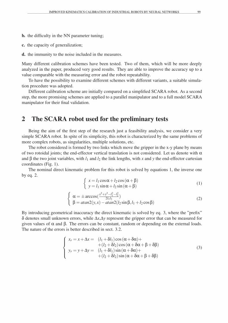
The robot considered is formed by two links which move the gripper in the x-y plane by means
of two rotoidal joints; the end-effector vertical translation is not considered. Let us denote with αand β the two joint variables, with l1 and l2 the link lengths, with x and y the end-effector cartesian
coordinates (Fig. 1).
The nominal direct kinematic problem for this robot is solved by equations 1, the inverse one
by eq. 2. {x = l1 cosα+ l2 cos(α+β)y = l1 sinα+ l2 sin(α+β) (1)
{α = ±arccos(x2+y2−l2
1−l22
2l1l2)
β = atan2(y,x)−atan2(l2 sinβ, l1 + l2 cosβ)(2)
By introducing geometrical inaccuracy the direct kinematic is solved by eq. 3, where the ”prefix”
δ denotes small unknown errors, while Δx,Δy represent the gripper error that can be measured for
given values of α and β. The errors can be constant, random or depending on the external loads.
The nature of the errors is better described in sect. 3.2.⎧⎪⎪⎨⎪⎪⎩
xr = x+Δx = (l1 +δl1)cos(α+δα)++(l2 +δl2)cos(α+δα+β+δβ)
yr = y+Δy = (l1 +δl1)sin(α+δα)++(l2 +δl2)sin(α+δα+β+δβ)
(3)
IMPROVED KINEMATICS CALIBRATION OF INDUSTRIAL ROBOTS BY NEURAL NETWORKS 99_________________________________________________________________________________________________________________

3 Calibration methodology
3.1 The Neural NetworkIn a problem of system identification (nonlinear input-output mapping) a right choice for a NN
is a multilayer feed-forward network, trained in a supervised manner with the back-propagation
learning technique [Haykin (1999)].
The chosen network contains just one layer of hidden neurons (Fig. 2) with sigmoidal activa-
tion functions. Linear activation functions are used for the output neurones. In accordance with
the ”universal approximation theorem”, this NN can approximate an arbitrary continuous func-
tion [Haykin (1999)]. Moreover, this choice is the optimum in the sense of easy implementation,
learning time and generalization.
(x,y)
X
Y
P
l1
l2
P2
P1
Motor 2
Motor 1
Tool center point
Figure 1: The SCARA robot joint variables.
Input level
Hidden level
Xi
Output level
Yj
Hk
W1ik
W2kj
1
1T1
T2 T2 T2
T1 T1 T1
b1k
b2j
� � � �
� � �
Figure 2: The feed-forward network used.
3.2 The tested calibration schemesThe authors attention has been focused first on the direct kinematic calibration and then on the
inverse one.
For the direct kinematics, the idea is to create a neuro-kinematic (NK) model of the real robot
(Fig. 3), merging a model of the ideal robot with a NN describing the manipulator errors. Different
schemes have been analyzed (Fig. 5) to select the more effective one.
In Fig. 3 we denoted as Qth = [α;β]t the values of the joint variables measured by the joint
transducers, while Sth = [x;y]t and Sre = [xr;yr]t are the theoretical and real gripper pose.
The NN is trained in order to reduce the quantity E = ‖Sre −SNK‖, which represents the error
in the gripper pose prediction, where ‖ · ‖ is the Euclidean norm.
The schemes of NK model in Fig. 5 enable the prediction of the actual gripper pose Sre, knowing
the joint rotations Qth (direct kinematics calibration).
IMPROVED KINEMATICS CALIBRATION OF INDUSTRIAL ROBOTS BY NEURAL NETWORKS100_________________________________________________________________________________________________________________

Figure 3: The direct kinematics calibration
model.
Figure 4: The inverse kinematics calibration
model.
For the inverse kinematics calibration is required to predict the joint rotation Qre that bring the
gripper of an actual robot in a desired pose Sth. A NK inverse model has to be trained (Fig. 4);
different possible schemes are shown in Fig. 6.
In order to make results comparable with those of the direct kinematics, instead of the joint error
E = ||Qre −QNK ||, as performance index was used the equivalent pose error E = ||ΔS|| = ||JΔQ||,where J is the jacobian matrix and ΔQ = Qre −Qth
4 Comparison of the different Neuro-Kinematics schemes
4.1 Angular coordinatesThe first simulations highlighted a problem related to large variations of the angles.
The robot behaviour depends on the sine and the cosine of rotation angles rather than on the angles
themselves. And so a rotation of α or α ± 2kπ produces the same effect. However, since the
NN activation functions are continuous and not periodical, if an angle is used as input to a NN,
the output value would be different when the input is α or α ± 2kπ. This fact makes the NN
behaviour unreliable for large rotation of the joint angles and for the representation of the gripper
attitude. After several tests, it was decided to replace each angular input of the NN with two
inputs representing the sine and the cosine of the angles, that means that the joint vector Q = [α β](trigonometric form) was defined as Q = [sinα cosα sinβ cosβ] (angular form).
A second aspect of this problem was the identification of the best way to add joint rotations in
the schemes like 2,3,4 and 6 of Fig. 5 and Fig. 6. This operation can be done in three different ways
as described in Tab. 1. In the preliminary tests, all the considered NN performed better using the
second type of angular addition.
Generalizing previous observations, every time a coordinates set X (X = Q or X = S) contains
some angular values, in order to avoid discontinuity and singularity, a transformation T (·) between
the angular form Xa and trigonometric one Xt have to be defined:
Xt = T (Xa) (4)
IMPROVED KINEMATICS CALIBRATION OF INDUSTRIAL ROBOTS BY NEURAL NETWORKS 101_________________________________________________________________________________________________________________

Figure 5: The direct Neuro-Kinematic
models tested
Figure 6: The inverse Neuro-Kinematic models
tested
IMPROVED KINEMATICS CALIBRATION OF INDUSTRIAL ROBOTS BY NEURAL NETWORKS102_________________________________________________________________________________________________________________
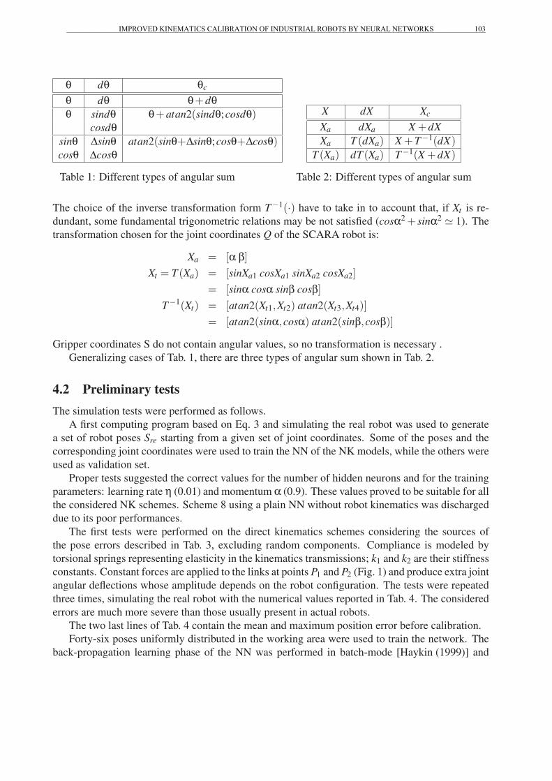
θ dθ θc
θ dθ θ+dθθ sindθ θ+atan2(sindθ;cosdθ)
cosdθsinθ Δsinθ atan2(sinθ+Δsinθ;cosθ+Δcosθ)cosθ Δcosθ
Table 1: Different types of angular sum
X dX Xc
Xa dXa X +dXXa T (dXa) X +T−1(dX)
T (Xa) dT (Xa) T−1(X +dX)
Table 2: Different types of angular sum
The choice of the inverse transformation form T−1(·) have to take in to account that, if Xt is re-
dundant, some fundamental trigonometric relations may be not satisfied (cosα2 + sinα2 � 1). The
transformation chosen for the joint coordinates Q of the SCARA robot is:
Xa = [α β]Xt = T (Xa) = [sinXa1 cosXa1 sinXa2 cosXa2]
= [sinα cosα sinβ cosβ]T−1(Xt) = [atan2(Xt1,Xt2) atan2(Xt3,Xt4)]
= [atan2(sinα,cosα) atan2(sinβ,cosβ)]
Gripper coordinates S do not contain angular values, so no transformation is necessary .
Generalizing cases of Tab. 1, there are three types of angular sum shown in Tab. 2.
4.2 Preliminary testsThe simulation tests were performed as follows.
A first computing program based on Eq. 3 and simulating the real robot was used to generate
a set of robot poses Sre starting from a given set of joint coordinates. Some of the poses and the
corresponding joint coordinates were used to train the NN of the NK models, while the others were
used as validation set.
Proper tests suggested the correct values for the number of hidden neurons and for the training
parameters: learning rate η (0.01) and momentum α (0.9). These values proved to be suitable for all
the considered NK schemes. Scheme 8 using a plain NN without robot kinematics was discharged
due to its poor performances.
The first tests were performed on the direct kinematics schemes considering the sources of
the pose errors described in Tab. 3, excluding random components. Compliance is modeled by
torsional springs representing elasticity in the kinematics transmissions; k1 and k2 are their stiffness
constants. Constant forces are applied to the links at points P1 and P2 (Fig. 1) and produce extra joint
angular deflections whose amplitude depends on the robot configuration. The tests were repeated
three times, simulating the real robot with the numerical values reported in Tab. 4. The considered
errors are much more severe than those usually present in actual robots.
The two last lines of Tab. 4 contain the mean and maximum position error before calibration.
Forty-six poses uniformly distributed in the working area were used to train the network. The
back-propagation learning phase of the NN was performed in batch-mode [Haykin (1999)] and
IMPROVED KINEMATICS CALIBRATION OF INDUSTRIAL ROBOTS BY NEURAL NETWORKS 103_________________________________________________________________________________________________________________
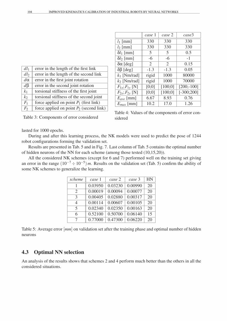
dl1 error in the length of the first link
dl2 error in the length of the second link
dα error in the first joint rotation
dβ error in the second joint rotation
k1 torsional stiffness of the first joint
k2 torsional stiffness of the second joint
F1 force applied on point P1 (first link)
F2 force applied on point P2 (second link)
Table 3: Components of error considered
case 1 case 2 case3
l1 [mm] 330 330 330
l2 [mm] 330 330 330
δl1 [mm] 5 5 0.5
δl2 [mm] -6 -6 -1
δα [deg] 2 2 0.15
δβ [deg] -1.3 -1.3 0.05
k1 [Nm/rad] rigid 1000 80000
k2 [Nm/rad] rigid 1000 70000
F1x;F1y [N] [0;0] [100;0] [200;-100]
F2x;F2y [N] [0;0] [100;0] [-300;200]
Eave [mm] 6.67 8.93 0.76
Emax [mm] 10.2 17.0 1.26
Table 4: Values of the components of error con-
sidered
lasted for 1000 epochs.
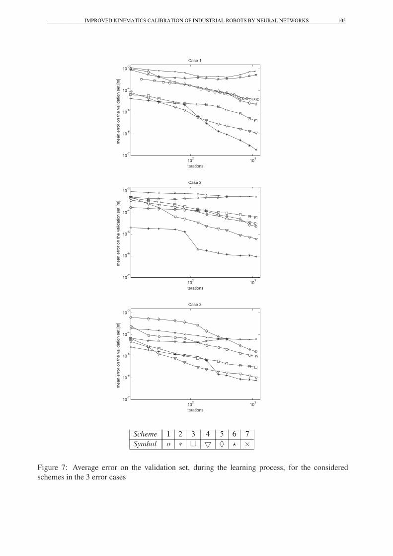
During and after this learning process, the NK models were used to predict the pose of 1244
robot configurations forming the validation set.
Results are presented in Tab. 5 and in Fig. 7. Last column of Tab. 5 contains the optimal number
of hidden neurons of the NN for each scheme (among those tested (10,15,20)).
All the considered NK schemes (except for 6 and 7) performed well on the training set giving
an error in the range (10−7 ÷10−5) m. Results on the validation set (Tab. 5) confirm the ability of
some NK schemes to generalize the learning.
scheme case 1 case 2 case 3 HN
1 0.03950 0.03230 0.00990 20
2 0.00019 0.00094 0.00077 20
3 0.00405 0.02880 0.00317 20
4 0.00114 0.00607 0.00105 20
5 0.02340 0.02350 0.00163 20
6 0.52100 0.50700 0.06140 15
7 0.77000 0.47300 0.06220 20
Table 5: Average error [mm] on validation set after the training phase and optimal number of hidden
neurons
4.3 Optimal NN selectionAn analysis of the results shows that schemes 2 and 4 perform much better than the others in all the
considered situations.
IMPROVED KINEMATICS CALIBRATION OF INDUSTRIAL ROBOTS BY NEURAL NETWORKS104_________________________________________________________________________________________________________________
102
103
10-7
10-6
10-5
10-4
10-3
iterations
mea
n er
ror o
n th
e va
lidat
ion
set [
m]
Case 1
102
103
10-7
10-6
10-5
10-4
10-3
iterations
mea
n er
ror o
n th
e va
lidat
ion
set [
m]
Case 2
102
103
10-7
10-6
10-5
10-4
10-3
iterations
mea
n er
ror o
n th
e va
lidat
ion
set [
m]
Case 3
Scheme 1 2 3 4 5 6 7
Symbol o ∗ � � ♦ � ×
Figure 7: Average error on the validation set, during the learning process, for the considered
schemes in the 3 error cases
IMPROVED KINEMATICS CALIBRATION OF INDUSTRIAL ROBOTS BY NEURAL NETWORKS 105_________________________________________________________________________________________________________________

First at all, schemes 1 to 5 using joint coordinates Q as input for the NN performed better with
respect to those based only on gripper coordinates S, probably because the same gripper position
can be reached with different values of the joint coordinates resulting in different pose errors.
Moreover, the parallel schemes (2,3,4,5 and 6) are preferred than the series ones (1,7); probably
because the NN has to learn just the difference between the nominal and the actual robot kinematics.
As already mentioned a scheme adopting only a NN without a nominal kinematic model was
rejected after the preliminary tests because its performances were clearly worse.
After all the tests the NK models 2 and 4 confirmed to be a good tool to predict the kinematic
behaviour of the actual robot. Few neurons were sufficient to reproduce the direct kinematics even
in presence of load deflecting the joints. These two schemes were selected for further tests.
4.4 Tests with random errorsAfter having identified the more efficient NK schemes, further tests permitted to verify the NN
behaviour in presence of noise or random errors like backlash.
All the poses constituting the training set were corrupted adding random errors with the max-
imum amplitude described in Tab. 6. E is the average pose error while the random component of
the pose error Er is computed as difference between the pose reached by the robot with constant
and random errors and the pose reached by the robot with only the constant part of the errors.
Then the NN of the NK models 2 and 4 were trained using the corrupted set following the
procedure denoted as ”early stopping method” [Haykin (1999)].
The number of training poses was dropped to 36 and the number of the neurons was experimentally
minimized in order to avoid the overfitting risk while keeping good convergence on the corrupted
training set.
Finally the average and maximum pose error were evaluated with respect to the validation set.
Results are reported in Tab. 7 for the direct kinematics and in Tab. 8 for the inverse one.
In this case for the NK schemes two performance indexes were evaluated: the ”actual error”
and the ”apparent error”. The actual error (Eac) is the error evaluated comparing the gripper pose
predicted by the NK model with the pose of the validation set not affected by random noise. The
apparent error (Eap) is the difference between the predicted poses and the poses of the validation
set corrupted by the random noise. It is important to note that Eac < Eap. In other words, the NN
reduces the effect of the random noise filtering it. With reference to the symbols of Tab. 6, 7 and 8,
we evaluated the filtering index as:
FI =Eac
Er(5)
Depending on the NK scheme, the filtering index was in the range 30%÷80%.
This result means that if the NN is trained using data having a certain amount of random error
Er, the apparent error in the validation set would be nearly equal to Er, but the actual error would
probably be much lower (30%÷ 80%) because the NN produces an ”average” effect on the data.
This is quite desirable.
The same considerations can be made for the inverse NK schemes: using the same values of
the errors of Tab. 6, the results obtained (Tab. 7, Tab. 8) show that schemes 2 and 4 are suitable for
inverse kinematic calibration too.
IMPROVED KINEMATICS CALIBRATION OF INDUSTRIAL ROBOTS BY NEURAL NETWORKS106_________________________________________________________________________________________________________________
parameters const randδl1 [mm] 5 ±0.1δl2 [mm] −6 ±0.12
δα [deg] 2 ±0.04
δβ [deg] −6 ±0.026
δx [mm] 0 ±0.01
δy [mm] 0 ±0.01
pose error ave. max.E [mm] 12.6 20.0
Er [mm] 0.17 0.49
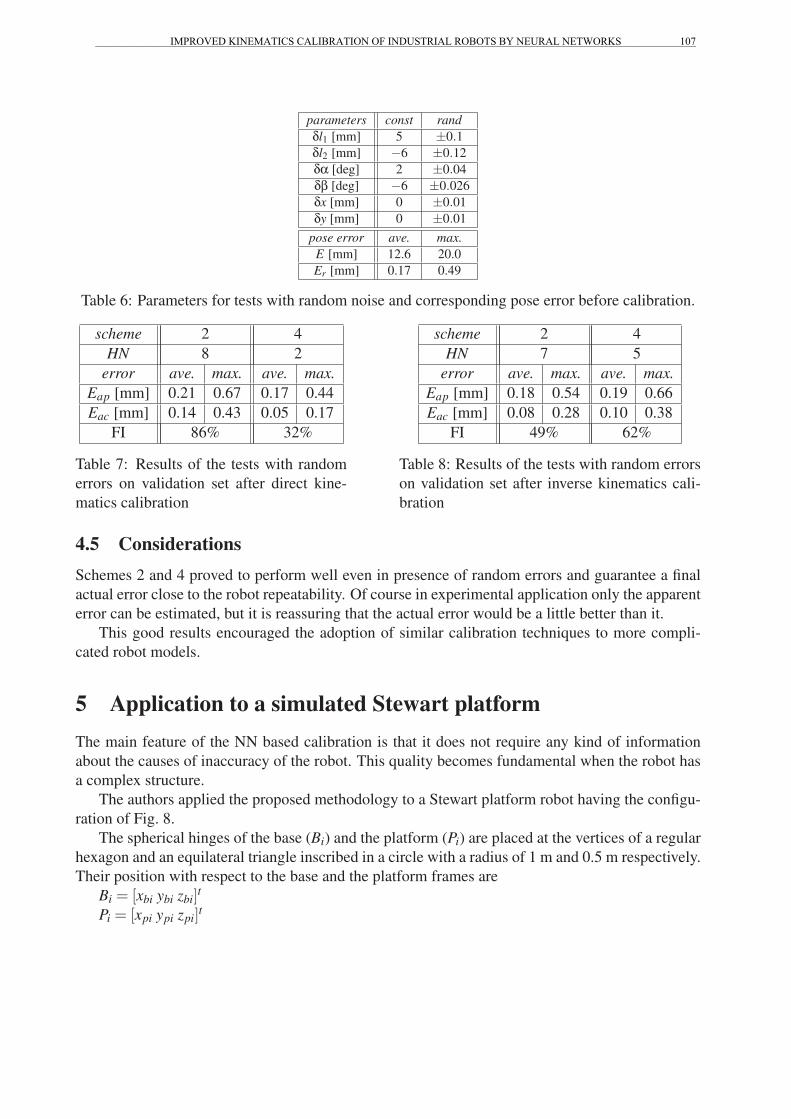
Table 6: Parameters for tests with random noise and corresponding pose error before calibration.
scheme 2 4
HN 8 2
error ave. max. ave. max.Eap [mm] 0.21 0.67 0.17 0.44
Eac [mm] 0.14 0.43 0.05 0.17
FI 86% 32%
Table 7: Results of the tests with random
errors on validation set after direct kine-
matics calibration
scheme 2 4
HN 7 5
error ave. max. ave. max.Eap [mm] 0.18 0.54 0.19 0.66
Eac [mm] 0.08 0.28 0.10 0.38
FI 49% 62%
Table 8: Results of the tests with random errors
on validation set after inverse kinematics cali-
bration
4.5 ConsiderationsSchemes 2 and 4 proved to perform well even in presence of random errors and guarantee a final
actual error close to the robot repeatability. Of course in experimental application only the apparent
error can be estimated, but it is reassuring that the actual error would be a little better than it.
This good results encouraged the adoption of similar calibration techniques to more compli-
cated robot models.
5 Application to a simulated Stewart platformThe main feature of the NN based calibration is that it does not require any kind of information
about the causes of inaccuracy of the robot. This quality becomes fundamental when the robot has
a complex structure.
The authors applied the proposed methodology to a Stewart platform robot having the configu-
ration of Fig. 8.
The spherical hinges of the base (Bi) and the platform (Pi) are placed at the vertices of a regular
hexagon and an equilateral triangle inscribed in a circle with a radius of 1 m and 0.5 m respectively.
Their position with respect to the base and the platform frames are
Bi = [xbi ybi zbi]t
Pi = [xpi ypi zpi]t
IMPROVED KINEMATICS CALIBRATION OF INDUSTRIAL ROBOTS BY NEURAL NETWORKS 107_________________________________________________________________________________________________________________

Six translational joints (Qi) link the platform to the base and control its position and orientation
(6 dof).
Three frames are used: frame {b} fixed to the base, frame {p} fixed to the platform and frame
{g} fixed to the gripper (translated with respect to {p} of zpg = 0.2 m). The gripper pose is defined
by the vector S = [xg yg zg ψ θ φ] (using Tait Brian orientation angles); the length of the six ”legs”
are used as joint coordinates Q = [l1 l2 l3 l4 l5 l6] = [Q1 Q2 Q3 Q4 Q5 Q6]t .The pose of the gripper with respect to the base is represented by the position matrix
Mbg = Trans(X ,xg) ·Trans(Y,yg) ·Trans(Z,zg)·Rot(X ,ψ) ·Rot(Y,ϑ) ·Rot(Z,φ) =
=
⎡⎢⎢⎣
cθcψ −cθsψ sθ xgsθcφ + cψsφ −sψsθsφ + cψcφ −sψcθ yg−cψsθcφ + sψsφ cψsθsφ + sψcφ cψcθ zg0 0 0 1
⎤⎥⎥⎦
the position of the mobile platform with respect to the gripper is
Mgp =
⎡⎢⎢⎣
1 0 0 0
0 1 0 0
0 0 1 −zpg0 0 0 1
⎤⎥⎥⎦
The inverse kinematic problem is easily solved: the positions of platform hinges [x′piy′piz
′pi]
t with
respect to the base frame {b} are computed using the transformation matrix Mbp which represents
the position of the platform frame with respect to the base one
Mbp = MbgMgp ⎡⎢⎢⎣
x′piy′piz′pi1
⎤⎥⎥⎦ = Mbp
⎡⎢⎢⎣
xpiypizpi1
⎤⎥⎥⎦
the leg’s length are computed as
li =√
(xbi−x′pi)2+(ybi−y′pi)2+(zbi−z′pi)2 (6)
i = 1 . . .6
The direct kinematic problem is solved using iterative numerical methodologies (extended Newton-
Raphson method).
Three different types of structural errors were added to this simulated robot:
• position error of the hinges of the base and the platform (δxi δyi δzi);
• length error of the legs (δli);
IMPROVED KINEMATICS CALIBRATION OF INDUSTRIAL ROBOTS BY NEURAL NETWORKS108_________________________________________________________________________________________________________________

• position (δxg δyg δzg) and orientation (δψ δθ δφ) error of the gripper with respect to the
platform.
The actual value of the geometrical parameters of the robot L is obtained adding three compo-
nents:
L = Ln +δLc ±δLr (7)
where Ln is the nominal (theoretic) value, dLc is the constant part of the error and dLr is the
random component which varies in each pose. Random component represents backlash and the
measurement tool uncertainty. For each geometrical parameter a value of the constant error Lc in
the ranges specified in Tab. 9 was randomly chosen.
δLc δLr
δxi δyi δzi [mm] ±1 ±0.02
δli [mm] ±3 ±0.02
δxg δyg δzg [mm] ±0.1 ±0.01
δψ δθ δφ [mrad] ±0.25 ±0.02
Table 9: Ranges of the constant (δLc) and the random (δLr) geometrical error values.
Inside the work space of the robot, defined as
−0.2 m < xg < 0.2 m−0.2 m < yg < 0.2 m
1.0 m < zg < 1.4 m−30 deg < ψ < 30 deg−30 deg < θ < 30 deg−30 deg < φ < 30 deg
50 poses (randomly distributed) for learning set (lea) and 100 for validation (val) were selected.
As a consequence of the (small) geometrical errors, the theoretical gripper pose differs from the
actual pose. The homogeneous matrix M that describes the roto-translation between them has the
following form
M �
⎡⎢⎢⎣
1 −Δφ Δθ ΔxΔφ 1 −Δψ Δy−Δθ Δψ 1 Δz
0 0 0 1
⎤⎥⎥⎦ (8)
Calibration has the aim of minimizing the difference between predicted and actual pose, i.e. min-
imizing the extra diagonal elements of M. To measure the pose prediction quality two different
error index were computed, the first for position, the second for orientation:
Exyz =√
Δx2 +Δy2 +Δz2 (9)
Eang =√
Δψ2 +Δθ2 +Δφ2 (10)
IMPROVED KINEMATICS CALIBRATION OF INDUSTRIAL ROBOTS BY NEURAL NETWORKS 109_________________________________________________________________________________________________________________

[mm] set E δLr δLr/2 δLr = 0
ave max ave max ave maxxyz 5.98 14.3 5.98 20.7 5.98 20.6
lea ang 9.60 17.1 9.34 20.5 9.34 20.5
δLc xyzr 0.10 0.26 0.04 0.14 0 0
angr 0.08 0.17 0.03 0.10 0 0
val xyz 5.99 28.8 6.47 50.0 6.48 50.1
ang 9.62 26.0 9.93 59.9 9.96 60.1
xyzr 0.11 0.60 0.05 0.40 0 0
angr 0.09 0.56 0.04 0.31 0 0
xyz 3.22 13.5 2.87 7.03 3.24 13.5
lea ang 4.88 12.3 4.62 7.12 4.88 12.3
δLc/2 xyzr 0.10 0.38 0.05 0.18 0 0
angr 0.08 0.27 0.04 0.13 0 0
xyz 2.93 9.91 3.10 25.3 2.93 9.76
val ang 4.70 10.5 4.86 24.7 4.70 10.1
xyzr 0.10 0.46 0.05 0.24 0 0
angr 0.08 0.38 0.04 0.23 0 0
Table 10: Pose errors for the Stewart platform before calibration (mm or mrand).
Average and maximum values on the validation set before calibration are shown in Tab. 10; to
highlight the effects of constant and random errors, simulation tests were repeated 6 times with
different combinations of the constant (δLc,δLc/2) and of the random (δLr,δLr/2,0) errors. In
Tab. 10 values labelled by xyz and ang are the average linear and angular error, while xyzr and angrare the random components.
Contrary to serial robots, in parallel ones a joint configuration Q can bring the robot gripper
in several different poses with different pose errors. This means that the robot configuration is
completely defined only when the pose vector S is known. However, in actual uses of parallel
robots, only one of the possible joint configuration is used because the change of the configuration
implies the crossing of a singularity (where the structure is under-constrained). With this restriction
even vector Q gives full information. For this reason, the calibration schemes that can be used are
2, 4 and 6.
Scheme 4 and 6 involve an angular sum on gripper coordinates S (orientation angles ψ,θ and φ).
In order to avoid singularities of Tait Brian angles (θ = ±π/2) and discontinuity across ±π the
transformation T (·) was built choosing eight elements of matrix Mbp and defining the angular Saand the trigonometric St form of S:
Sa = [x y z ψ θ φ]t
St = T (Sa) = [x y z cθcψ − cθsψ
sθ − sψcθ cψcθ]t
= [St1 St2 St3 .̇. St8]t
Sa = T−1(St) = [St1 St2 St3 atan2(−St7,St8)asin(St6) atan2(−St5,St4)]t
Pose error after calibration of the inverse kinematics are shown in Tab. 11. The average actual error
on the validation set was strongly reduced but not enough to reach the repeatability of the robot Er:
for this reason the filter index FI is greater than 100%.
The proposed calibration methodology applied to a 6 dof robot had worse performance than the
IMPROVED KINEMATICS CALIBRATION OF INDUSTRIAL ROBOTS BY NEURAL NETWORKS110_________________________________________________________________________________________________________________

2 dof SCARA. It is important to notice that NN’s learning is, practically, an interpolation proce-
dure so the density of the poses in the training set is a main factor for a good performance. If the
robot has several dof, a great number of measured poses are necessary to cover the n-dimensional
work-space of the robot (with n=dof).
Some comments are: the pose errors after calibration in the validation set is 2 or 3 times that of
the calibration set having the same initial value of constant and random error. The two considered
schemes have in average the same performances: the average accuracy error is reduced from some
millimeters to about 0.1 mm. The presence of the random error significantly degrades the calibra-
tion performance.
[mm] set E δLr δLr/2 δLr = 0
ave. max. ave. max. ave. max.xyz ap .074 .203 .054 .118 .026 .078
lea ang ap .160 .504 .111 .299 .061 .190
xyz ac .066 .182 .054 .110 .026 .078
δLc ang ac .142 .501 .108 .338 .061 .190
xyz ap .133 1.03 .112 1.49 .087 .737
val ang ap .327 3.40 .282 5.15 .225 2.47
xyz ac .123 .924 .111 1.55 .087 .737
ang ac .304 3.01 .280 5.32 .225 2.47
FI xyz 132% 217% -
ang 386% 669% -
xyz ap .040 .114 .019 .036 .010 .023
lea ang ap .101 .320 .041 .106 .025 .077
xyz ac .039 .098 .021 .049 .010 .023
δLc/2 ang ac .084 .280 .044 .121 .025 .077
xyz ap .096 .384 .045 .258 .032 .115
val ang ap .198 1.19 .107 .755 .086 .465
xyz ac .083 .046 .040 .246 .032 .115
ang ac .173 1.50 .097 .689 .086 .465
FI xyz 217% 86% -
ang 669% 258% -
Table 11: Pose errors after inverse kinematics calibration of the Stewart platform using scheme 2.
6 Full SCARA model
The set of structural errors used for the SCARA robot simulated in the previous case was not
complete. This means that not all possible geometrical inaccuracy were considered for the simu-
lated robot. In order to test the NN based calibration methodology with a full robot model, a 3 dof
SCARA manipulator was used.
The kinematics model is shown in Fig. 9: reference frames are positioned on the robot using
Denavit & Hartenberg conventions.
In a generic serial robot the number of geometrical errors is
N = 6+4R+2P (11)
were R is the number of rotational joint and P the number of translational one. However, de-
pending on the measuring instrumentation, just some of them can be estimated. Assuming that G
IMPROVED KINEMATICS CALIBRATION OF INDUSTRIAL ROBOTS BY NEURAL NETWORKS 111_________________________________________________________________________________________________________________

[mm] set E δLr δLr/2 δLr = 0
ave. max. ave. max. ave. max.xyz ap .039 .087 .025 .057 .021 .053
lea ang ap .080 .178 .056 .182 .051 .174
xyz ac .039 .092 .026 .054 .021 .053
δLc ang ac .085 .286 .061 .155 .051 .174
xyz ap .115 .659 .068 .648 .081 .832
val ang ap .287 2.01 .161 2.24 .183 2.41
xyz ac .103 .600 .064 .559 .081 .832
ang ac .264 1.62 .153 1.94 .183 2.41
FI xyz 110% 125% -
ang 336% 366% -
xyz ap .033 .108 .030 .076 .010 .033
lea ang ap .084 .382 .066 .417 .022 .110
xyz ac .032 .066 .030 .087 .010 .033
δLc/2 ang ac .068 .227 .067 .256 .022 .110
xyz ap .073 .259 .071 .213 .041 .303
val ang ap .143 .750 .160 1.28 .095 1.05
xyz ac .061 .160 .061 .383 .041 .303
ang ac .113 .505 .149 1.18 .095 1.05
FI xyz 60% 131% -
ang 137% 395% -
Table 12: Pose errors after inverse kinematics calibration of the Stewart platform using scheme 4.
Figure 8: Simulated Stewart platform. Figure 9: Simulated 3 DOF SCARA.
coordinates of the gripper pose can be measured the number of the identifiable parameters is
N = G+4R+2P (12)
Eq. 11 and Eq. 12 are obtained generalizing the concepts described in [Mooring et al.(1991)]. Since
we assumed that only the position (x y z) of the gripper could be measured (and not its orientation),
the number of geometrical error parameters which have to be defined to describe the robot geometry
is N = 3+4 ·2+2 ·1 = 13.
A complete set of parameters describing the 3 dof SCARA geometry and compliance was se-
lected [Omodei et al. (2000), Legnani et al.(2001)]. Nominal values and errors of the geometrical
and compliance parameters are shown in Tab. 13 and Tab. 14 respectively.
A force F , whose components are function of the pose coordinates was applied to the gripper
causing joint and gripper deflections (Tab. 15).
Fx = c1x+ c2xy+ c3z
IMPROVED KINEMATICS CALIBRATION OF INDUSTRIAL ROBOTS BY NEURAL NETWORKS112_________________________________________________________________________________________________________________

L Ln δLc δLr
X0 trans(Xb) [mm] 0 2.5 ±0.02
Y0 trans(Yb) [mm] 0 −2.2 ±0.02
χ0 rot(Xb) [mrad] 0 2.3 ±0.02
ψ0 rot(Yb) [mrad] 0 −1.7 ±0.02
θ1 rot(Z0) [mrad] Q1 −1.7 ±0.02
a1 trans(X0) [mm] 330 0.4 ±0.02
α1 rot(X0) [mrad] 0 0.1 ±0.02
ψ1 rot(Y0) [mrad] 0 −0.3 ±0.02
θ2 rot(Z1) [mrad] Q2 0.7 ±0.02
a2 trans(X1) [mm] 330 −0.4 ±0.02
α2 rot(X1) [mrad] 0 0.2 ±0.02
ψ2 rot(Y1) [mrad] 0 1.7 ±0.02
d trans(Z2) [mm] Q3 0.1 ±0.02
Table 13: Geometrical parameters of the 3 dof SCARA.
L Ln δLc δLr
Kxy [m/N] rigid 10−5 ±10−6
Kz [m/N] rigid 10−5 ±10−6
Kθ1 [rad/Nm] rigid 10−5 ±10−6
Kθ2 [rad/Nm] rigid 10−5 ±10−6
Kd [m/N] rigid 10−4 ±10−6
Table 14: Compliance parameters of the 3
dof SCARA.
Ln δLc δLr
c1 0 3 ±2
c2 0 -6 ±2
c3 0 12 ±2
c4 0 -15 ±2
c5 0 30 ±2
c6 0 3 ±2
c7 0 6 ±2
c8 0 -18 ±2
Table 15: Coefficients of Eq. 13: forces in [N]
distances in [m].
Fy = c4x2 + c5xz (13)
Fz = c6 + c7z+ c8xy
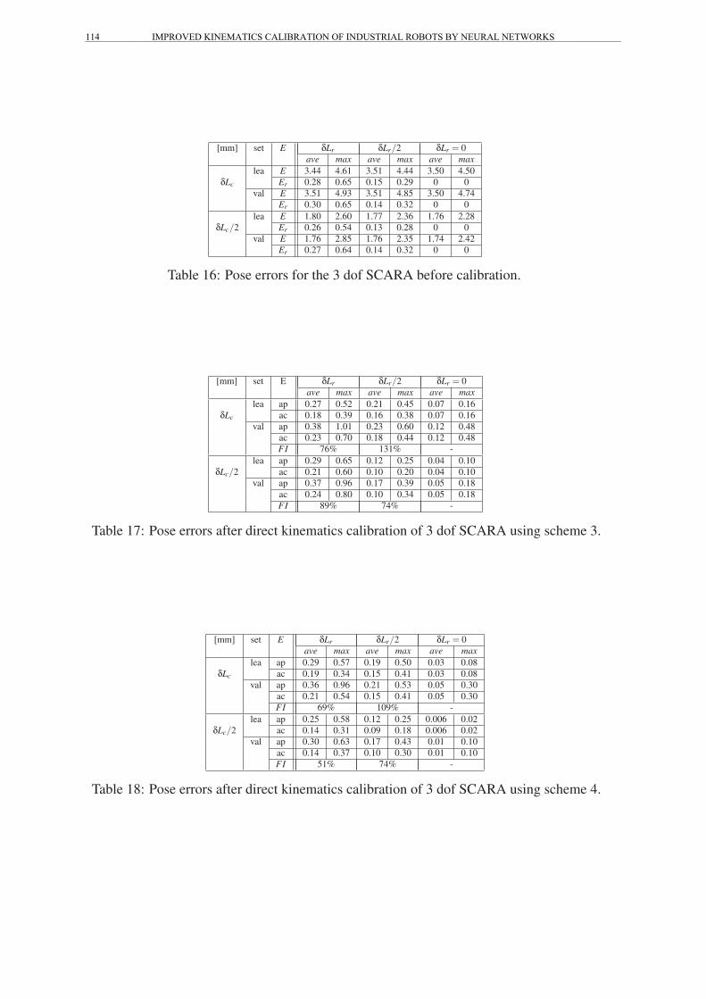
Inside the work space (which has a torus shape Rint = 0.13 m, Rext = 0.53 m, 0 m < z < 0.3m) 72 uniformly distributed poses for the learning set (lea) and 430 for the validation set (val) were
selected. The pose error is computed using Eq. 9. Average and maximum values of the pose error
E and the random component Er before calibration are shown in Tab. 16. To better analize the
properties of the calibration technique in different situations, the algorithms have been tested with
different combinations of constant (δLc) and random (δLr) errors values.
Apparent and actual pose error after direct kinematics calibration using scheme 3 and 4 are
shown in Tab. 17 and Tab. 18 respectively. Gripper coordinates don’t include angular values, so no
transformation T (·) is needed.
Results reported in Tab. 16, Tab. 17 and Tab. 18 show that the calibration procedure proposed
IMPROVED KINEMATICS CALIBRATION OF INDUSTRIAL ROBOTS BY NEURAL NETWORKS 113_________________________________________________________________________________________________________________
[mm] set E δLr δLr/2 δLr = 0
ave max ave max ave maxlea E 3.44 4.61 3.51 4.44 3.50 4.50
δLc Er 0.28 0.65 0.15 0.29 0 0
val E 3.51 4.93 3.51 4.85 3.50 4.74
Er 0.30 0.65 0.14 0.32 0 0
lea E 1.80 2.60 1.77 2.36 1.76 2.28
δLc/2 Er 0.26 0.54 0.13 0.28 0 0
val E 1.76 2.85 1.76 2.35 1.74 2.42
Er 0.27 0.64 0.14 0.32 0 0
Table 16: Pose errors for the 3 dof SCARA before calibration.
[mm] set E δLr δLr/2 δLr = 0
ave max ave max ave maxlea ap 0.27 0.52 0.21 0.45 0.07 0.16
δLc ac 0.18 0.39 0.16 0.38 0.07 0.16
val ap 0.38 1.01 0.23 0.60 0.12 0.48
ac 0.23 0.70 0.18 0.44 0.12 0.48
FI 76% 131% -
lea ap 0.29 0.65 0.12 0.25 0.04 0.10
δLc/2 ac 0.21 0.60 0.10 0.20 0.04 0.10
val ap 0.37 0.96 0.17 0.39 0.05 0.18
ac 0.24 0.80 0.10 0.34 0.05 0.18
FI 89% 74% -
Table 17: Pose errors after direct kinematics calibration of 3 dof SCARA using scheme 3.
[mm] set E δLr δLr/2 δLr = 0
ave max ave max ave maxlea ap 0.29 0.57 0.19 0.50 0.03 0.08
δLc ac 0.19 0.34 0.15 0.41 0.03 0.08
val ap 0.36 0.96 0.21 0.53 0.05 0.30
ac 0.21 0.54 0.15 0.41 0.05 0.30
FI 69% 109% -
lea ap 0.25 0.58 0.12 0.25 0.006 0.02
δLc/2 ac 0.14 0.31 0.09 0.18 0.006 0.02
val ap 0.30 0.63 0.17 0.43 0.01 0.10
ac 0.14 0.37 0.10 0.30 0.01 0.10
FI 51% 74% -
Table 18: Pose errors after direct kinematics calibration of 3 dof SCARA using scheme 4.
IMPROVED KINEMATICS CALIBRATION OF INDUSTRIAL ROBOTS BY NEURAL NETWORKS114_________________________________________________________________________________________________________________

is very effective in the reduction of the positioning error. By using both scheme 3 and 4 the error is
reduced to values close. For the considered manipulator the best results are achieved by scheme 4.
As observed for the 2 DOF SCARA robot, the NN partially filters the random errors.
7 Conclusions
The paper presents a preliminary study on an innovative Neural Network based calibration pro-
cedure. Different schemes of a Neuro-Kinematic model were tested in direct and inverse kinematic
calibration both on serial and parallel simulated robots. Three of them obtained good performances:
in all considered cases accuracy error was reduced nearly to robot repeatability. It was also shown
that the NK model is able to filter part of the noise component present in the measures.
The NN based procedure seems to be suitable to the calibration of all robot types and extremely
simple to use: only the nominal kinematic model of the robot is needed, the procedure is able to
compensate for all type of ripetitive errors present in the robot (geometrical, load deflections, ...)
without modelling them.
Similarly to other procedures, a proper (quite large) number of measured poses distributed in the
workspace (or in a part of it) is needed. The results obtained in the simulated cases encouraged the
authors to apply the proposed procedure to actual robots.
References[Nowrouzi et al.(1988)] Nowrouzi A., Kavina Y.V., Kochekali H., Whitaker R.A., An overview of
robot calibration techniques, Ind Robot, pp. 229-232, 15(4), 1988.
[Zierteg and Datseris (1989)] Zierteg J., Datseris P., Basic considerations for robot calibration, Int
J Robot Aut 4(3), 1989, pp.158-166.
[Mooring et al.(1991)] Mooring B.W., Roth Z.S., Driels M.R., Fundamentals of manipulator cali-
bration, New York, 1991.
[Kovac and Frank (1992)] Kovac I., Frank A., A novel industrial robot calibration device, Proc. of
First RAA, Porotoz, Slovenia, pp. 162-167, 1992.
[Faglia et al. (1993)] Faglia R., Legnani G., Magnani P.L., Docchio F., Minoni U., Calibration of a
SCARA robot by optical measurements: Methodology and experimental results, ISMCR’92
2nd Int Symp on Measurement and Control in Robotics, Sept. 21-24, 1993.
[Legnani et al.(1996)] Legnani G., Mina C., Trevelyan J.P., Static calibration of industrial manip-
ulators: Design of an optical instrumentation and application to SCARA robots, J Robot Syst,
13(7), 1996.
[Trevelyan et al.(1996)] Legnani G., Trevelyan J.P., Static calibration of industrial manipulators:
a comparison between two methodologies, Robotics Toward 2000 Twenty-Seventh Int Symp
on Industrial Robots, pp. 111-116, Oct. 6-8, 1996.
[Khoshzaban et al.(1996)] Khoshzaban M., Sassani F., Lawrence P.D., Kinematic calibration of
industrial hydraulic manipulators Robotica v.14, pp. 541-551, 1996.
IMPROVED KINEMATICS CALIBRATION OF INDUSTRIAL ROBOTS BY NEURAL NETWORKS 115_________________________________________________________________________________________________________________

[Haykin (1999)] Haykin S., Neural networks: a comprehensive foundation, Prentice hall, 1999.
[Omodei et al. (2000)] Omodei A., Legnani G., Adamini R., Three Methodologies for the Cali-
bration of Industrial Manipulators: Experimenthal Results on a SCARA Robot J. of Robotic
System 17(6), pp. 291-307, Wiley, 2000.
[Legnani et al.(2001)] Legnani G., Adamini R., Jatta F., Calibration of a SCARA Robot by Force-
Controlled Contour Tracking of an Object of Known Geometry, 32nd ISR, Korea, Apr. 19-21,
2001.
[Tiboni et al. (2003)] M. Tiboni, G. Legnani, P. L. Magnani and D. Tosi, A closed-loop neuropara-
metric methodology for the calibration of a 5 DOF measuring robot, Proceedings of the
IEEE Int. Symp. on Computational Intelligence in Robotics and Automation, July 2003, Kobe
Japan, pp 1482- 1487.
[Fazenda et al. (2006)] Fazenda N., Lubrano E., Rossopoulos S., Clavel R. Calibration of the 6
DOF High-Precision Flexure Parallel Robot Sigma 6, Proceed. of the 5th Chemnitz Parallel
Kinematics Seminar, Chemnitz, April 25-26, 2006.
IMPROVED KINEMATICS CALIBRATION OF INDUSTRIAL ROBOTS BY NEURAL NETWORKS116_________________________________________________________________________________________________________________

�
�������������������� ��������������� ������������������� ��� ��������
��
������������� ������������������������������������ �������� ��� ���� ���������� !!����������"��������!��#���#����$��������
����% ����&��$��� ���'$�(�!�� ���% )���$��������
�
������������������������� ������������������������������������������������������� ���������������������� ��� � ��� ������ ���� �������� ��� ������� �������� � � ������� �������� ����� ����� ������������ � � ��� �� ���� �������� ��� ������� ������� ��� � ���������� ������� ������ ��� �� � ����� ������ ��� ������ ������ ���� ����������� � � ������������ ���� ������ ������������������ ������������������ ��������� �������� ��������� ���������������������� � �������������� ��������������������������������������� �� � ������� ��������� ��������������������������������������������������������������������� ��������������� �������������������������� � ����������������!������������������������������������������������� � ������� ��� ���� ����"�� ������!�������� ������� ����� �� �������� � ����� ���� ���� ��� �������������������#�������� ���#������� ������������� � ���� �������������(�����*��������!�*�������*���+� ������������������!� �����++��������!���!+���������!�+ �����!��++�� ���� �� ���� ���� + ���!!�� %��� *������� + ���!!� �!� ���� ������ *���� ���� ��� ��!� ��#� �+ �����!��������� �������� ��,���!���������*�������� ��������������������)�����%�� ��� ������+ �����!� � �� ���� ���� !���� !�)�� ���� �� ���� ���� � ����*������� + ���!!��%��� ���� � ������� �����+��,� + ������ �!� ��� ����� �� ���� ����� �� +� ����� �� ���� ���� ���+� ��� ��� ����� !��+�� ���� � ����*�������+ ���!!� �!� ����!�����%���!!� �� �����++ �+ ����������!���!���� ����*������ ������� ���������������*�������+ ���!!�����+ ���!!���!������!������� �����������-���������������-����������� ���������������������*�������+ ���!!���!������� ������������ ����������*���������!+����*����������� �+����������!!������+ ���!!������������'�����+����� ��� ��� ������������ ���� ��� !�!����*���� ����� ����� ����� ��!���� �� � ���� ������
���������� ��!�� + �!������ ��� ���!� +�+� � �!� !����!!������ �����+��!���� ��� ���� ���� ��� ��������!� ���� �++���������� .�� !+���� ��� ���� ��!� �!�� ��� *� �!� ����� ��� ���� +�!�� ��� �� ��*��++��������� ��� ���� ����� ��!���� �!� ������ *���� �� ��������� � + ������*����� ������!� �� � ���������������,+� �����*�������,+� �����!���������������!�/% �������01123�4�!��"��01125���.�� ���������������� ��!���� ���� ��� ����� �!!������ + ���!!� ������!� ��� ���� ���������� ����
��� ���������� ��� ���� +� +�!�� ��� ���� �++��������� *����� �!� �!������ ���� ����� ���� + ������ ������!� ������������ ��� ��+ ������+� ����� !�������� ��!�� �������������!�����������������������!������ ��������� ��� ������� �!!������ ��� *� �� !� ��!��� ��� ���-����� !��+���� %��� ���� ���!�!���� ���!��� ��� ��� ���!� +�+� � ��!�� *� �� ��!�� ��� ���� ����!� ���� ���� ������� *�� �� ������������������ ���������,+��!�!�� �������������.��������!!������+ ���!!�!��������� ���+ ���!!��!�!�������������*� �� !��%����� ����+�����
�������� �!��������� ���� #�������� ������ �� + ������ � � �� +� �� ���� ���� ���� !��+�� ������ �!����
INNOVATIVE ACCESSION TO THE RING MEASUREMENT IN THE CONTROL PROCESS USING MACHINE VISION 117_________________________________________________________________________________________________________________

�
+� !�����!�����!!����-�������������� ���������!���!���!��������������!����!�!�����%�����!�!�� ���!���������+��,������������� ��������!+������+���!����*� �� 6!�+!������������+��!����������������%������!�-�����!�� ����� �!�*� ���� �!���!����������+�!!�������������� �����������������!��%��� ������������������������!���!��!���� ��!�����!�������������������� ����!!����%����7!� �������� ��!���� !�!���!� � �� �� �� ���� �� �� �������� ���� ���!�� ���� ��� ��� ��
����������� �� � ����!� ���� �++��������!� ���� � �� ��������� ����!+��!����� ��� �!!������ + ���!!�/8 �����!�'��01125��9��� ��� !�!���!���!����������������!����� �� ��+��������+� �� ��������� ���+ ���!!�������� �������������������������������������������!��� �����++ �+ ������!������������������������!��������������!����� ���!!� �����%��� �������� ��!���� !�!���� ������ �!��� ��� ����!� ���� ���� ������� �� � ��!�!� !���� �!�
��!+����������!� ����������������������������!��������� ���!�������� �� ��������!�!������� ������ ��!�������������+�����+ ���!!�����������!� �������-��+������!��������������!������!���������*�������,���+ ����� ��/% �������01123�4�!��"��01125��:!����������+ ����� ���!�!+���������+ ���!������ ��������������!�!�/���!� �������������������5���������!����������������!�������+������ !��������� ���� *� ����� ���������!� /������������� +�!������ ���� ��������5����+������ !��������� ��� �������� ��!���� /���� �� ���+��� � ���!�!� ���� �+���!5� ���� ��������������+���������������������+� �� ��������������!�!�������%��!�+�+� ��!�����!����������������+��������������������������� �����*������!����+�������
�����+��� �!���*� ��+ �� ����!������� ��������� ������%������!�������������������� ������!���!�� �����+������� �����������+������������������������� ���!�!����� �����������������+�+� ����������!�!������!�!���6!�-������� �!�+ �!������������!��!!���*�� �� �� �������� ��������!�������� ��� !�!���!;� ���� ������� �,+� �������� ���� ����!� ���� �++��������� � �� ���+� ��� ������!��!!�������� �����������������������.�� ���� ����!� ���� ���� *������� + ���!!� ���� ������ + ������ -������� ���� ��� �+ �!���!� �������!� �������������� ����� ������!!������*������ ����*����� �!� ����� ������ ����� ������ ��� ��!!�������+� ��������9��� ��� + ���!!� ��� ���� ���� ������� � ���� ������!!� �����*!� ���� + �����!� + ���������
+ ���!!�!� ����� �������� ���� �*� ���� ���� �������� ���� *������� ���� ����� .�� ���� ����������+ ���������+ ���!!�!������� �������������!��������� ��$�������!���� �������!���������� �������� �+�������������������!� ����������$%%�+� ��������� ���+ ���!!�!������������ ���������,�!����� -������� ���� ��� + ����� �� ��� ����*������ ���� �������!� ��!���� ��!� ����� ��� ���� �
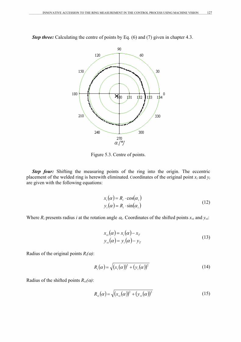
!� ����� ��� *������ ���� *�� �� ���� ��!� � ��� �!� +�������� :!���� ���� ����� �� �� � �����!��������������������!��* �������� + ����������� ���� ���6!����� �����"����������� �������������� ���� ����!������������������������� ��%�����,������������ � ������!��������!��� ���������!�!����������%��!��� ������������� ��!��!��� ���� �������������������������� ���������!�!�����!�����������!�������� ����!��%��� ������� ���� ����� �� � ���!� ���� !���*� �� + �� ��� ���� �� ���� ��!���������� ���
�,+� �������� !�!���� �!���� ���� �������� ��!���� � �� ������+��� �� � ���� ������ �����������++�������������+ �!������������!�+�+� ��%������� ���+ ���!!��������!����!� ��������;�
�� ������� �&��/���!� �������� ����'%�%(��� �+�����������'%�%$��5��� ������!!�)��/���!� �������� ����'%�*(��� �+�����������'%�%(��5�
�%����������������,+���������������!� ����+� ����� !�� ��!��*�������� ������������0�<��%��� ����!��+��������� �����!�!��*���!������������������ ���������������/&���5�������,�����
INNOVATIVE ACCESSION TO THE RING MEASUREMENT IN THE CONTROL PROCESS USING MACHINE VISION118_________________________________________________________________________________________________________________

�
/&��5� ������� !� ��� ���� ���� � �� !��*�� �!� �*�� ��*� ������ �� ��!�� %��� ����� ����� ���*������,������������������������ � �+ �!���!� ������!!�������� ����/)�5����
����� ��0�<��= �+������+ �!���������������!� ���� ������ ����
�� �������������������������%��� ���!� ���� !�!���� �!� +������ ��� �� !+������� +�!������ �����!���� ��� ���� � ��!+� ������� �����/������� �����5��%�������� >�<�+ �!���!������ ���� ��� ���������+�!!��������!�*�� �����!� ����!�!�����!����������������������������������� ������� ��/�� ���������011?5����
��
���� ��>�<��(��������������*��������������!����!�!�����
INNOVATIVE ACCESSION TO THE RING MEASUREMENT IN THE CONTROL PROCESS USING MACHINE VISION 119_________________________________________________________________________________________________________________

�
%���*������ �����!�������������� ������ ��� �������� ��!+� ������������������� ������������������������� � !���� /��������)���5��%��� �������� ������ �!�+������ ��� ����+ ���!�� ������+�����+����� �!��*����������>�<��!��� ����/"�����&��011<3�(���� �� �������<@A25��������� ���+�����!� ��� ��+����� ��!���� !�!���� �!��� ��!�� ��� + �!������ ���!� ���� !�!���� � ��/$��� ��&��01115;��� ���� �!��������� �����!�!��� ������)� !�/�����������������:$85��� ������!�� ��!��� ��������������!� �������B�����+�����������!+������!��� .CD��� �*� ���� + ���!!��������!��� ��!����!���*� ���
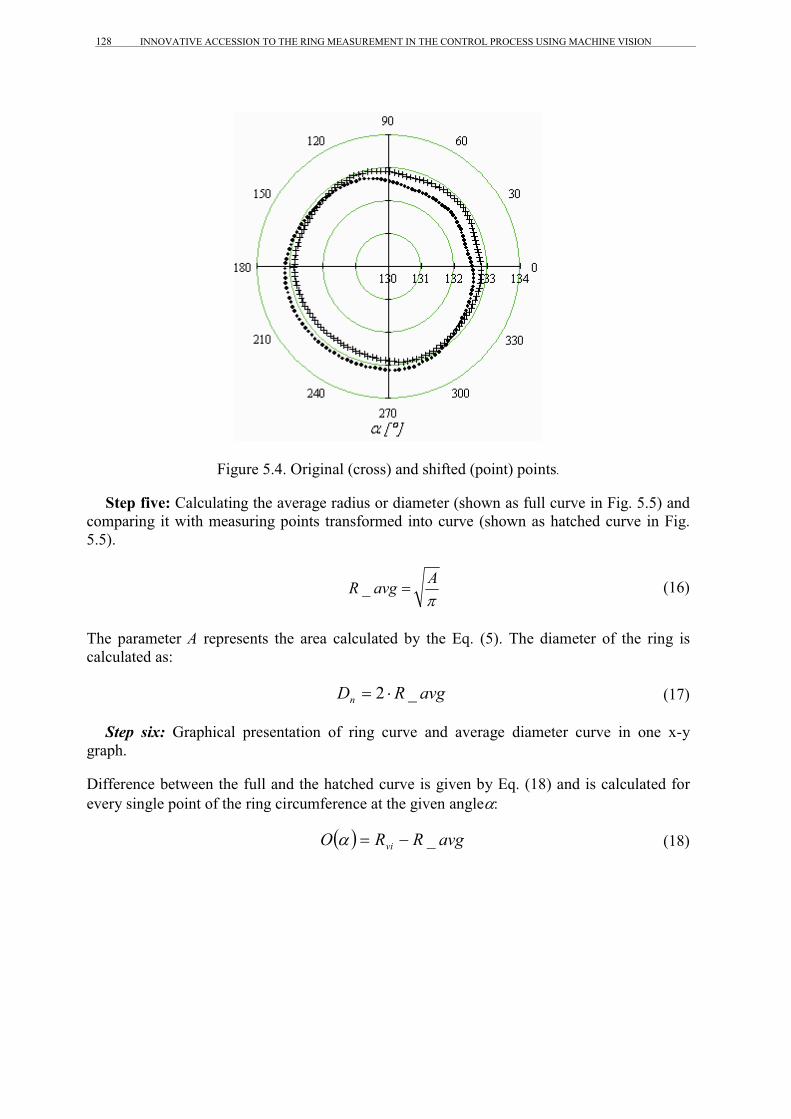
�%������!� ����+ ����+����������������� ��������� ������!!��������*������ �����!�!��*����������>�0��%������!� ����������!�!�!������������ ������������!� �!�� ���*������ �������������������,�������� ��%���*������ �����!���,���������� ���������������!�!��*����������>�0���
����� ��>�0��%������!� ����+ ����+����
�4�������� �����!� ���������������� ���!����������!��+!����/� ������5������� ��+�,���� ��!�������� ��������������!������$%%�+����!�� ���������� ���������� ��������� ���������� � ������������������ � ������� ���!�� "��������� � ��������������� ���%�����!��!���� ������!� � � �������������������� �� �+ �!������������!����+�� ��%�����!� � ����!��� ������ ��� ���� ��!���� ��� ���� ���� !� ����� �!� !��*�� ��� ����� E�<� !�� ��� �!� +�!!����� ��� ���� �����!� ������������������� ���+������%���������� ���+������!���!� ������������� ��*�������!������� !��� �+� �� ������� � +%� ��� ,%� ��� ��� ������ ���*���� ���� �� ���� ��!� � ��� �!� ������� ������������+���������������!�/= ���� ��011<3����������<@A?5��.������*������ �����!� �������
INNOVATIVE ACCESSION TO THE RING MEASUREMENT IN THE CONTROL PROCESS USING MACHINE VISION120_________________________________________________________________________________________________________________

�
������!� ����������� �+������!������������������ ����!�� ���!� � ����� �������� ���+� ����� !�*������ ����������� ���� �������������������������������� ��!��*����������E�<����������E�0���
��
���� ��E�<��" ����+��!������!� �� ���������������������%��� � ��!�� ������� �-������� �� � ���� + �!������ � ������������ ������� *����� ������!� ��������������������� ����� �������+ �����!�����������+� ����� !��!���������������-��/<5;���������������������������������������������������������������� � � ���� �� ��� < � /<5��9��!��� ���������-��/<5�����!�+�!!������������������������������������ ����/��5�������*��������+� ����� !���� /��������������������� ��!� � ��5��$� /�����,� ���������+�!��������� ������!� � ����!����� �!���������� �����5������ ��!�� ������������ ���*���������������������������!���������-��/05�/!��������E�05����
�������������������������������������������������������������������� � �� � � /05�
�
��
���� ��E�0���������!+���;�*�������!� �����!�������� ����!� �������+�� �������������� ���
INNOVATIVE ACCESSION TO THE RING MEASUREMENT IN THE CONTROL PROCESS USING MACHINE VISION 121_________________________________________________________________________________________________________________

�
%������� ��������+ �!��������������������!+��������������+��� ��!�!��*����������E�0��%�����!� � ���!��*���!���*������� ������������!�������� ����������������� ������ �+ �!����������������� !���������������+ �������*��*���������!�� ��!���������������!� ����/!�������E�05��%���� �+ �!���������,� ���� ��������������+�!���������������!� � ���*��������� �����!� �������������!�� � ������������������ � ����������������#����$�%���!�!����*������!���!� ���������������!�������������*���������!;�
�� ���� ���������,������ ���������������!�������*������������!���������!��� ����*������ ������������ ��������������� �� �+ �!�������!� �����������
��� !�� ������������� ��� �������!� ���� +����� �� � ���� ������ �� ���� � ���� ��!� ��� ��� �,+�������*�� �� ���� ���� �� ��� ���� ���� �!� +������ ���!���� ��� ���� �������� �,���� .�� �!� ���� � ����� ��� ��������!� �����++�������������!���+�!!��������+���������*������ �����,������������� ���������,������4�������� �����!� ���������������� ��������� �����!������������������� ��� �#���� ���!�!��*��
��������E�>���� � ���!���!�� ���� ��!� � ������ � ������!� ���� ��!� �+����������������� ���� ���� �!� �+ �!����������-��/>5�*�� ��-��� � �+ �!���!����� ������������ �������������+��������� ������� ������������������
��
���� ��E�>��.������� ���� � �������� ������!����������� ���������,������
���������������������������������������������������� � � � �00 !����! ���� .-.- ��� ����� � />5��
.�� F�������� ���� ����G��H�-/�� F� ����!���� ����G��H�
������;�
0� F� ��������������GIH��.�������E�E����� �!���!��������+����!�-��� ��������������������-��/>5�� ��+ �!������� �+���������.�� ������,��!��+� ���� ������������� ���������� ���+�!��������� ��!� � ������ ����������� ������� �!��,+��������%���� �������!����������++�� !������*��������+�!���������������!� ��!����������� �������� ��������������� ����/�� �����������!� ����+ ���!!5��
INNOVATIVE ACCESSION TO THE RING MEASUREMENT IN THE CONTROL PROCESS USING MACHINE VISION122_________________________________________________________________________________________________________________

�
��
���� ��E�E��$��������+����!�-��� ����%��������� ���+�!���������������!� ��!�!��*����������E�J��.��������!� �+�!�������!����������� �
������!�������1����� ���������������������������������-��/E5���
��
���� ��E�J�������� ���+�!���������������!� �B������������������������� ����������
���������������������������������������� � � � �00 !����! 1.-.- ���1 ������ ��� � /E5��������;� 1� F�������� �+�!�����������!� � ���G��H��
INNOVATIVE ACCESSION TO THE RING MEASUREMENT IN THE CONTROL PROCESS USING MACHINE VISION 123_________________________________________________________________________________________________________________

�
����� ��E�2��9��+� �!������*��������(�/�5���������()/�5��
�9��+� �!��������������������������!��������������� ������!�-��� �����-1�� ����������+��������������� �����������������!�!��*����������E�2������!�� ������������ ������� �������������� � ��������������� � �����%�������� ����� ��� �������!� ���� ���� ����� �!� ��� ���������� ���� � ��� ���� ���� ���� �� ��� ���!�
� ���*������!����� �����������!� ����+����!�����������*��������!��K��*������������������������� ���� ����� ���� � ��� ��� �!� +�!!����� ��� ���������� ���� ������ ���+������������ ���� ������� ���� ���������������%��� �� ��� �!� +������ ��� *&� +����� *�� �� ���� 2� �+ �!���!� ���� ����� ��� ���� � ��� ���� 2�
�+ �!���!�������!�������������!� ����� ���/!��������E�?5���
����� ��E�?�� ������,F����� �������!�!�����
��
.�� ���� � ��� �!� ���!� ���������+����!� �������������� ������� � ��� � �����+������� /����� E�A5� ����� ���2�����������������������-��/J5�/�� #�����%��011E5���
INNOVATIVE ACCESSION TO THE RING MEASUREMENT IN THE CONTROL PROCESS USING MACHINE VISION124_________________________________________________________________________________________________________________

�
����� ��E�A�� ������!� �������������!�*����+����!���������� �� !��
��
�������������������������������������������������������� � �� ���
3
��� ����2 ���� �
�
��� <
<
<<0
<� /J5�
�"� ����� !��������� �+ �!������� ������!�����������!� ����+������%������� ���������� ���/�������5��!����������������-��/25�����/?5�/$��������0112F011A3�8� ���"��<@AA5���
������������������������������������������������������������������������������������� 24� �
�
L
� � /25�
�
������������������������������������������������������������������������������������� 24
� ��
L
� � /?5�
�45
������45��� ��!��������������!����!� ������� ��� ��������������,�!�����������-��/A5�����/@5�
/$��������0112F011A3�8� ���"��<@AA5;��
����������������������������������������������� � � � ���
���� ������
<
<<
0<
0<
L
2< 3
�������� ������4 � /A5�
�
���������������������������������������������� � � � ���
���� �������
<
<<
0<
0<
L
2< 3
�������� ������4 � /@5�
��%� &������� �������������� ������������%�������������������!� �������� ��������!�!�!����!�,�!��+!����
����� ���� = ������� ���� ���!� ���� +����!�� %��� !�������� +����!� !��*�� ��� ����� J�<� �+ �!���� ���� ��!������ ��������� ��� ���� ��!� � ����� � ��������� ��� ���� ���6!� !� ����� *����� �+ �!���!���������� ���+������������� ������!!��������*������ �����%����-����������������!� �� �������������!��!��;��������������������������������������������������������������������� � � ���� �� ��� < � /<15�
INNOVATIVE ACCESSION TO THE RING MEASUREMENT IN THE CONTROL PROCESS USING MACHINE VISION 125_________________________________________________________________________________________________________________

�
��
���� ��J�<�����!� ����+����!���
����� ���%���+����!�� ������������*���� ����!����� ���� ����!��� �������-M���!��� �!��!���/�-��<<5����
������������������������������������������������������������ �� �������-- �� M � /<<5��%����� �����������!��!��� ����� �������������� ����!����
��
���� ��J�0��9� �������������� ���+����!��
INNOVATIVE ACCESSION TO THE RING MEASUREMENT IN THE CONTROL PROCESS USING MACHINE VISION126_________________________________________________________________________________________________________________
�
�����������9������������������� �����+����!�����-��/25�����/?5�������������+�� �E�>���
��
���� ��J�>��9��� �����+����!���
����� ���� $�������� ���� ���!� ���� +����!� ��� ���� ���� ����� ���� � ������ %��� ������ ���
+����������������*������ �����!��� �*����������������9�� ������!��������� �������+���������������� ��������*�������������*�����-������!;���
���������������������������������������������������������������� � � �� � � ����
���
-�-�
����
!����!����
� /<05�
�4�� ��-��+ �!���!� ����!���������� ������������������9�� ������!��������!�������+����!������������;���
���������������������������������������������������������������� � � �� � � � ����
����
������
����
����
� /<>5�
�(����!��������� �������+����!�-��� ;��������������������������������������������������������� � � � �� � � �� �00 ��� ��� ��- �� � /<E5��(����!��������!�������+����!�-���� ;��
������������������������������������������������������� � � � �� � � �� �00 ��� ������ ��- �� � /<J5��
INNOVATIVE ACCESSION TO THE RING MEASUREMENT IN THE CONTROL PROCESS USING MACHINE VISION 127_________________________________________________________________________________________________________________
�
��
���� ��J�E��D �������/� �!!5�����!�������/+����5�+����!���
'�� ��(�9������������������ ���� ����!�� �������� �/!��*���!�������� �����������J�J5��������+� ���� ���*�������!� ����+����!� � ��!�� ���� ������� ���/!��*���!����������� ��� ��������J�J5����
������������������������������������������������������������������2��- �M � /<25�
�%��� +� ����� �2� �+ �!���!� ���� � ��� ����������� ��� �����-�� /J5�� %��� ������� � ��� ���� ���� �!�������������!;���������������������������������������������������������������� ��-&� M0 �� � /<?5�
������ ����= �+������ + �!��������� ��� ���� �� ��� ���� ��� ���� ������� � �� ��� ��� ���� ,F��
� �+����'���� ��������*������������������������������� ����!�����������-��/<A5������!�������������� ���� ��!������+������������ ������ ����� ������������������������;������������������������������������������������������������ � � ��--) �� M��� � /<A5��
�
INNOVATIVE ACCESSION TO THE RING MEASUREMENT IN THE CONTROL PROCESS USING MACHINE VISION128_________________________________________________________________________________________________________________

�
��
���� ��J�J�� �� �������� ����������� ��� ��!����%�����������F�)��������������,�����F�)�������� ��������*�������!���*���� ��!��!��!����� ����������������� ������!!�������� ����F�)��/&��4��N��������=��O��9����011J5���
����������������������������������������������������� � � �� � � ���--)
��--)
��
��
M��,M���
��,
���
����
��
� /<@5�
�������������������������������������������������������� � � � ��� ��,��� )))� �� � /015��= �+���� �,+��������� ��� ���� ���� ������!!� �!� !��*�� ��� ����� J�J�� (������!!� ��� ���� ������+�������������� �����������������!�!��*��������������J�2����
����� ��J�2��(������!!���� ������+�������������� ���������������������GIH��
INNOVATIVE ACCESSION TO THE RING MEASUREMENT IN THE CONTROL PROCESS USING MACHINE VISION 129_________________________________________________________________________________________________________________

�
)� �����������������.���� � �!�� ������������*�����,+� ����������!�!�� ���!��;��� ���� �!+��!����������� �����!� �+�!�������� ���+� �!���������� �!���!��!���� ����� ������������� ������!��� �+������������������+� ��+����������� ���������������������� ����+�!�����!����������� �!���!����+� �!���*�������� ����*����+� �!��
�D����������!���*����!�!�� ��+ �!������������!�+�+� 6!��,+� �������� �!���!���.�� ���!� �!�� ��� ���� ���!� ���� �!���!� ���������� ��� �� ��� !�!���!� �!���� ���� !���� ��!�������������������� ������ �����+� ����%����� !�������!� �+ �!�������� ������!��������� �������!�!����*�� ����!�������������������� ������!��!���*������������� ������!��%����$��,������������9���+ �� ��!�� ���!����� ������������!������ �+�����������)�!�������)!�(�(�!���!������������ �������!�!�����
6�������������7��8�
9������������7��8�
(����������� � 1�110�B�1�1>A�/1�105�(���� ������!!� 1�1<A�B�1�1J>�/1�<5�
��%��� !������ !�!���� �!� �+ �!������ �!� ���� �,+� �������� ���� *�� �� ��!��� ����������������� ����� �!� �����+��!���� ��� ����!!� �� �� ������!� �� � ���� ����� + �� ��� ������� P�!����8�!����� ��++��������!�/% �������01115��%��� �!���!��������������� �����������%���2�<���9� ������!;�����������������,�� ������� �����!����������������������� �����!���������������)!�(�(�!���!���������,+� ��������!�!�����
6�������������7��8�
9������������7��8�
(����������� � 1�110�B�1�1<@�/1�105�(���� ������!!� 1�11J�B�1�1EJ�/1�<5�
�%������ ��!�!�����!� �+ �!�������!���������!� �����++���������*�� ����������!!� ���� ������!�� ���!��������+ �������� �+�������������� �!���!�������)!�(�(�!���!��������!� �����++����������
6��������������7��8�
9������������7��8�
(����������� � 1�11J�B�1�1<�/1�105�(���� ������!!� 1�11J�B�1�1E�/1�<5�
��%���� �+������+ �!��������!�������� �!���!���� ���� ����������� ��������� ���� ������!!��� ������� ���!�!���!�� ��!��*����������2�<����������2�0���
INNOVATIVE ACCESSION TO THE RING MEASUREMENT IN THE CONTROL PROCESS USING MACHINE VISION130_________________________________________________________________________________________________________________

�
%����� !��� �+��������������2�<� �+ �!���!����� �+������������������ ����������� ����!� ���������� ���� !������ � �+�� ��� ���� ����� 2�0� �+ �!���!� ���� �+����������� ��� ���� ���� ������!!����!� �������%����� ���� �+����!�!��*��������!� ���� �!���!� �� � ���� ���� �������!�!���� ����� ������� �+����!��� ������,+� ��������!�!������������-��� �����+����!��� ���������������!� ����!�!�������%��� �������� ����� ��� ����� 2�<� ���� ����� 2�0� !��*!� ���� ������ ��� ����� � � ���� ���� !�������� � ���!�����������!� ����!�!����� �!������������ ��� �����!�����������������+�� �0������
��
���� ��2�<��(�+��������������������� ����!� ��������
�
��
���� ��2�0��(�+�������������� ������!!����!� ���������
INNOVATIVE ACCESSION TO THE RING MEASUREMENT IN THE CONTROL PROCESS USING MACHINE VISION 131_________________________________________________________________________________________________________________

�
*� ������������.�� ����+ �!������+�+� ����� �!�� ���*� ���!�����!����������������+�����������������������F����� ����� ���� ����� *����� �!� ��������� ��� ���� �� ����� ��!���� ���!� ���� !�!����� %�������������!���� �,+� �������� !�!���� �� � ���� ����������� � ���� ���� ������!!����!� ������*�!���!��������+������%��� �!���!����������!����!!���� �+���������������������/��������*� �� !5�-����������� ���
���*������ ���!����������������!�������� ���*�����������!������ �������������������� ����������� ����-����������� ���+ ���!!��� ������������������������+� ��������+����������������� ����!��#�������������#���������!�� �����!�� ������!�����������������������!�������� ����������+�*���� ���� ������)������ ��� ���� + ��������!� ����� � ������ *�� �� ���� ������ *� �� *���� �����,��������������� ����-����������� ���*���������������!�� �����%��� �,+� �������� �����!�!� ��� ���� �!���!� �!� + �!������ �� � �� ��� !�!���!�� %��� � -�������
��+���!�������� ������������������ �+�������������� �!���!��%������� �������!�!�������!����� �����������!���� 6!� �-��!��!������!�!�����!������������������� ������� ��������!� �����++����������%����,+� ��������!�!�������+ �!�!�������+ ��������� ����������� �����*�� ������ �!���!�������� �+������������ ������������ ��%��!�*�!������� !��!��+��������� ������������ ������������!� ����!�!�����%��� ����!� ���� !�!���� ��!� ����� ������������ ���!� ������� ��!� ������������� ��!� �����+ ����������������!� ������������!���!����+� ��� ���!�������������%����,+� �������� �!���!�+ �������������-����������� ���*������� ����������������������!����
������������!� ����+ ���!!��������*������ ������+���!�������� �������������������������-��!����� ���� ��+�� ��� ����������� ���+�����!� ��� ���� !�!���� ���!� ������ ���� ����� ��������������������������#�������+� ��,��-�������%����,+� ��������*� ��*�!�������������������+�����$'�(�!�� ���/ �������!����!�!����
+ ����� 5�� ���$������������
�.� / �����8� ���"��<@AA3�9����������%��� ��� ���9��� ����D�� �"������3�&����<@AA�
8 �����!�'��01123�P�!������������ ��!!����������������� !!������ ����������0�2C0�/01125�+���<A<�B�<A>���
= ���� ��011<3�9���� ����������� ����������������� �!�������+��� ���!���3�8� ����$+ ���� �011<�
���������<@A?3�D+���!3� ���!��F4�!����<@A?�
�� ���������011?3�9��+��� ���������������!�����!������ ��������!!������+ ���!!�&�� ������������������������� ����.��J>�<0C011?�!� ��AJAFA?<�
&��4��N��������=��O��9����011J3�(������!!�� � ��!!�!!����3�.�!����������+��!��!�"����!�����<>C011J�
INNOVATIVE ACCESSION TO THE RING MEASUREMENT IN THE CONTROL PROCESS USING MACHINE VISION132_________________________________________________________________________________________________________________

�
�� #����� ��%� ��=��011E3� ������� �������� ����!� ������������������ ��������3��=�����!�����!�����EAC011E��
"�����&��011<3���� �����B�8�!���(�����P�!���3�$+ ���� �011<�
(���� �� �������<@A2;�(����!�����!!������D+���:���� !����" �!!�<@A2�
$��� ��&��01113�$��������������!� ����+ �����!��!������������������!�����!��������� !�����++��������'$�(�!�� ���
$�����=����������0112F011A3��"����������� ���!��������� �!3��=��!+������ ����!�!�0112F011A�
% �������01113�P�!����%����������!������� ��.�!+���� !�% �������9�� !����'$�(�!�� ���
% �������01123�(��������!� �������� �������+ �����!����+;CC***���! �!�� ���!��
4�!��"��01123� �(�����+��� ��������������������P�!����$�!���3� ���������P�!����$�!����.����
INNOVATIVE ACCESSION TO THE RING MEASUREMENT IN THE CONTROL PROCESS USING MACHINE VISION 133_________________________________________________________________________________________________________________

Deformable and Rigid Objects Grasping
Mihai Stoica, Gabriela Andreea Calangiu and Francisc Sisak Department of Automatics, “Transilvania” University of Brasov, Romania
Abstract In this paper we consider the problem of real manipulation in a realistic environment – a flexible fabrication cell. In the first parts of the article are presented some methods for automatic grasp planning using a three-finger manipulator. Information presented here consist of a method for automatic grasp planning using shape primitives, a vision-based method used for grasping extruded objects and an algorithm used for grasping deformable objects. In the last section, is presented a general algorithm used for grasping deformable and rigid objects in flexible fabrication cells. 1 Introduction
Selecting a good grasp of an object using an articulated robotic hand is a difficult problem because of huge number of possibilities. One way of limiting the large number of possible hand configurations is to use grasp pre-shapes. Before grasping an object, humans unconsciously simplify the task to selecting one of only a few different prehensile postures appropriate for the object and for the task to be performed. Medical literature has attempted to classify these postures into grasp taxonomies. Cutkosky and Wright (Cutkosky M.R., 1986) extended this classification to the types of grasps need in a manufacturing environment and examined how the talk and object geometry affect the choice of grasp. A number of papers present contact-level grasp synthesis algorithms (Ding D., 2000; Ferrari C., 1992; Hester R.D., 1999; Itu A., 2007). These algorithms are concerned only with finding a fixed number of contact locations without taking into consideration the hand geometry. Other systems built for use with a particular hand, restrict the problem to choosing precision fingertip grasps, where there is only one contact per finger (Hester R.D., 1999). These types of grasps are good for manipulating an object, but are not necessarily the most stable grasps because they do not use inner finger surfaces or the palm. Most robotic systems currently in existence have been built under the assumption that manipulation of rigid objects remains the primary task. In reality though, many objects are non-rigid. Most are unsymmetrical, compliant, and have alterable shapes. Ayanna Howard and George Bekey developed an algorithm for handling of 3-D deformable objects. They defined a ‘3-D deformable object’ as an object whose three flexible degrees of freedom are characterized by viscoelastic interactions between molecules (Howard A.M., 2000).
Even for a simple three-fingered hand, such as the Barrett Hand, there are a total of 10 degrees of freedom: 6 degrees of freedom in placing the wrist relative to the object and 4 internal degrees
DEFORMABLE AND RIGID OBJECTS GRASPING 134_________________________________________________________________________________________________________________
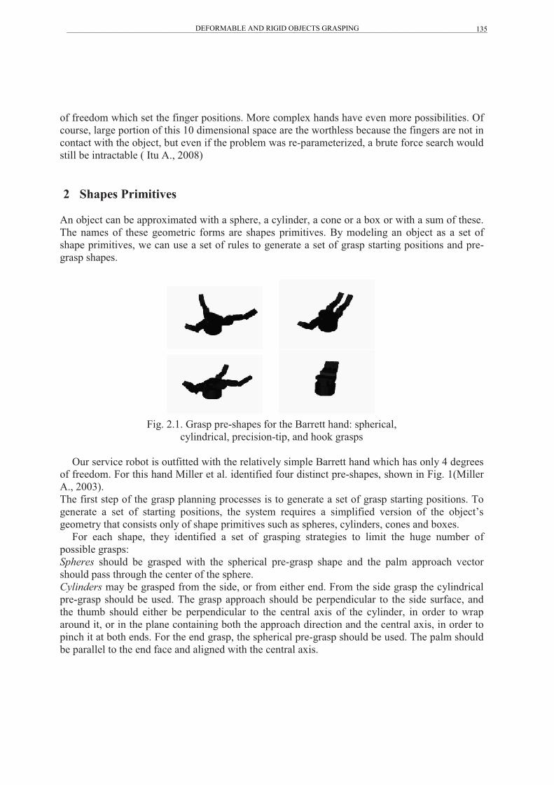
of freedom which set the finger positions. More complex hands have even more possibilities. Of course, large portion of this 10 dimensional space are the worthless because the fingers are not in contact with the object, but even if the problem was re-parameterized, a brute force search would still be intractable ( Itu A., 2008) 2 Shapes Primitives
An object can be approximated with a sphere, a cylinder, a cone or a box or with a sum of these. The names of these geometric forms are shapes primitives. By modeling an object as a set of shape primitives, we can use a set of rules to generate a set of grasp starting positions and pre-grasp shapes.
Fig. 2.1. Grasp pre-shapes for the Barrett hand: spherical,
cylindrical, precision-tip, and hook grasps
Our service robot is outfitted with the relatively simple Barrett hand which has only 4 degrees of freedom. For this hand Miller et al. identified four distinct pre-shapes, shown in Fig. 1(Miller A., 2003). The first step of the grasp planning processes is to generate a set of grasp starting positions. To generate a set of starting positions, the system requires a simplified version of the object’s geometry that consists only of shape primitives such as spheres, cylinders, cones and boxes.
For each shape, they identified a set of grasping strategies to limit the huge number of possible grasps: Spheres should be grasped with the spherical pre-grasp shape and the palm approach vector should pass through the center of the sphere. Cylinders may be grasped from the side, or from either end. From the side grasp the cylindrical pre-grasp should be used. The grasp approach should be perpendicular to the side surface, and the thumb should either be perpendicular to the central axis of the cylinder, in order to wrap around it, or in the plane containing both the approach direction and the central axis, in order to pinch it at both ends. For the end grasp, the spherical pre-grasp should be used. The palm should be parallel to the end face and aligned with the central axis.
DEFORMABLE AND RIGID OBJECTS GRASPING 135_________________________________________________________________________________________________________________

Cones can be grasped in the same ways as a cylinder. However, in the case of a cone with a large radius and small heath, the side grasps will be very similar to a grasp from the top. To handle this, we have added as set of grasps around the bottom rim of the cone, where the palm approach vector is aligned with the bisector of the angle between the bottom face and the side face. Boxes should be grasped using the cylinder pre-grasp shape, such that the two fingers and the thumb will contact opposite faces. The palm should be parallel to a face that connects the two opposing faces, and the thumb direction should be perpendicular to the face it will contact. 3 Three-finger Grasp Synthesis of the planar objects using Vision This chapter presents a practical approach for synthesizing three-finger grasps on planar unknown objects by means of vision. It is used visual perception to reduce the uncertainty and to obtain relevant information about the objects.
An important element of grasp synthesis is contact stability. Contact stability includes those aspects that involve the contact of a single finger against the surface of the object (Molares A., 2004). First they need define a practical criterion that encompasses the contact stability constraints. This is the finger adaptation criterion. It evaluates the fitting of the gripper’s finger against the object surface in terms of the estimated contact area. The criterion establishes that the object’s surface curvature must not exceed a threshold α̂ (curvature threshold) for being considered stable. The contiguous regions on the contour that comply with the finger adaptation criterion are called grasp regions: those having curvature under α̂ for all their points. The grasp regions are determined by grouping consecutive points with absolute curvature below the curvature thresholdα̂ .
Finally, each grasp region is abstracted as a straight segment called grasp region segment. These segments are computed from the line defined by the minimal square fitting of the points of the region, bounded by the first and last points of the region. Ideally, it should be possible to approximate these regions as straight lines The use of such an abstraction of grasp regions has important practical implications. First, the use of grasp regions discards those points with a high curvature, that is, with an unstable contact. And second, the use of grasp regions reduces the complexity of the problem of converting a contour composed, potentially, of hundreds of point, to a few grasp regions. This allows for the combinatorial techniques of the further stages to perform their computations in a reasonable amount of time. For grasp synthesis Molares et al. defined the force-closure criterion with the goal of characterizing force-closure grasps using three fingers. The purpose of this criterion is to ensure that the gripper does not cause the object to slide due to a torque when it closes its fingers to grasp it. The evaluation of this criterion is based on the concept of friction cone. A sufficient condition for reaching force-closure with three fingers is that the intersection of the friction cones of the three contact points is not empty, and that the unit normal vectors to the surface defined by the contact points positively spans plane. (Molares A., 2004). Three vectors positively span the plane if any of them can be written as a positive combination of other two (see figure 3.1).
DEFORMABLE AND RIGID OBJECTS GRASPING 136_________________________________________________________________________________________________________________

Fig. 3.1. The grasp (a) achieves force closure, whereas the grasp
(b) does not In a more formal way n vectors niui ...1, = span the plane if and only if:
�≠=
=>∃=∀n
jijjjij ucucnii
,1,0,...1, (3.1)
The goal when constraining a three-finger grasp is to find a configuration of the hand such that the positions of the three fingers is the same as in the original grasp, and the orientation of forces exerted by the fingers are similar. This problem can be very complex since the description of the configuration is composed by a lot of parameters that have to be determined. Antonio Morales and Pedro J. Sanz developed a procedure which consists of fixing the contact points of the hand configuration in the same location as the three-finger grasp. This, along with the constraints imposed with the hand kinematics, reduces the problem to a more tractable one. 4 Grasp Planning for Deformable Objects For the problem of grasping for non-rigid objects, in the first step it must to calculate deformation characteristics for object and in the second step, it must calculate the minimum force required to successfully lift the object. If wF is the force required to lift a rigid object of weight W with frictional coefficient μ , we define the minimum deformable object lifting force fL as dw FF + where dF is a minimum additional force term required to compensate for the deformation of the object. At the sub-microscopic scale, all solid material is composed of atoms. Adjacent atoms in a solid exhibit both attractive and repulsive forces which keep the atoms at equilibrium distance from each other. Deformation of a material is caused at the microscopic level by visco-elastic
DEFORMABLE AND RIGID OBJECTS GRASPING 137_________________________________________________________________________________________________________________

interactions between atoms. This visco-elastic interaction can be modeled by the Kelvin Model which is characterized by a spring and damper in parallel. Zhao et al. have utilized this model and have characterized a deformable object as a set of particles locally interconnected by damped springs (Zhao X.C., 2008).
The mathematical model for deformable objects is presented in the following. Let nf represent the external force applied to particle nψ . Let nm represent the mass of the particle nψ . Let nS represent the number of damped springs connected to particle nψ . Based on the mathematical equations defining the Kelvin Model, the forces acting on the nth particle are accumulation of external force, inertial force, damping force and spring force. Using Newton’s law of motion, the partial differential equation of motion for the nth particle can be written as:
nn
S
iinin
nin
S
iinn
inS
in
ftfpD
tftp
tft
pm
n
nn
=Δ
+∂
Δ∂+
∂Δ∂
�
��
=
==
),(
),(),(
1,,
,
1,2
,2
1
λ
(4.1)
where nD , the deformability coefficient, is a function of the force and the change in spring length, nλ , the damping coefficient, is a function of the force and the instantaneous change in spring
length, inp ,Δ represents the change in spring length in each Cartesian direction, and ),(, tftp
nin
∂Δ∂
represents the instantaneous change in spring length. From equation 4.1, we see that the only parameters which are not directly defined as a function of time are the mass, deformability, and damping coefficients. If we assume that the mass of the object is given, then we can classify the overall deformation of the object in terms of the deformability function D and the damping function λ . For determining the deformability function are used the following steps:
1. Apply a force against the object’s surface. At time nm tttt ,...,, 10= , record the force )( mtf 2. Calculate the particle displacement vector )),(( mm ttfd for all ttm ∈
3. The deformability function is )),((
)(),(mm
m
ttfdtfdfD = for all ttm ∈
The damping function is determined in the same mode. The difference is that here is calculated the particle displacement velocity vector.
To learn the characteristics of an adequate grasp, we must determine the relationship between mass, deformation and force. The steps required to handle manipulation of 3-D deformable objects are as follows:
1. Record dimensions of a known object 2. Calculate the deformability and damping functions 3. Determine the minimum force necessary to grasp known object by iteratively lifting
object 4. Links object attributes and grasping force into an index table.
DEFORMABLE AND RIGID OBJECTS GRASPING 138_________________________________________________________________________________________________________________
5 Algorithm used for grasping deformable and rigid objects 5.1 General requirements for using efficiently the algorithm This algorithm is used for grasping objects in a flexible cell, where should be placed a robot arm. This robot arm has attached a three-finger manipulator. Near this cell must be placed the conveyor. On the conveyor’s pallets deformable and non-deformable objects must be placed. The robot must grasp these objects and place them, for example into storage. Each pallet must have a certain code; some of these codes are used for identifying deformable objects and the other are used for identifying the rigid ones. Using the codes of the pallets the robot knows that the object which must grasp is deformable or rigid. In this cell must be placed a vision system with two cameras and a laser sensor. The vision system helps robot to detect objects contour, locate it and extract some features to match with predefined grasping models. 5.2 The algorithm used for grasping The algorithm has two important parts. The first one consists in learning an adequate grasp for deformable objects. The grasping for non-deformable objects does not need to be learned. The second part is, in fact, grasping of objects. The steps for learning an adequate grasp for deformable objects are presented below:
1. Determine deformability and damping coefficient for the deformable object which must be grasped. These coefficients are computed in the mode presented in the 4th section.
2. Determine the minimum force necessary to grasp known object by iteratively lifting object.
3. Weight the object with a balance placed under the conveyor’s belt. 4. Memorize, into an index table, the relationship between mass, deformability, damping
and force required for lifting. 5. Resume the algorithm from the first step and learn this relationship for the objects made
from the same material, but with the different weight. After that it can be determined a characteristic between mass and force (damping and deformability are known). Using the interpolation, we have to compute the lifting force, for a certain type of object after we know the mass of the object.
6. Resume the algorithm from the first step for all types of deformable objects. If we learn to grasp all deformable objects we can pass to the last part of algorithm: the effective grasping. The grasping steps of the objects are presented below:
1. Read the code of pallet and establish what type of object is, deformable or non-deformable.
2. If the object is deformable then go to the next step. If the object is non-deformable one, then give to the force-closure of the gripper the maximal value and, after that, go to step 7.
3. Weight the object. 4. Use the mode presented in the 4th chapter for determine the deformability and damping
coefficient. 5. For known mass, deformability and damping coefficients, extract the lifting force from
the index table. 6. Give the force-closure this value.
DEFORMABLE AND RIGID OBJECTS GRASPING 139_________________________________________________________________________________________________________________

7. Using the vision system to determine if the object is an extruded one or have a shape similarly with shapes primitives presented in the 2nd chapter.
8. If it is an extruded one go to the next step. If not, go to the step 13. 9. Measure the object’s height with a laser sensor and establish the grasp height at 2/3 of
object’s height from for the object with them height less than a predefined value or to a predefined height value for the rest of the objects.
10. Determine grasp regions from the 2D image of the object. 11. Take a combination of three regions and verify if these regions offer a stable grasp. If this
is a good one, grasp the object using the gripper kinematics and the computed lifting force. Then, go to the step 15. If is not stable go to the step 12.
12. Go to the step 10. 13. Determine which primitive shape can be used. 14. Grasp the object using the determined primitives shape on the step 13, compute lifting
force and gripper kinematics. Go to the next step. 15. Finish.
6 Conclusions Grasping has a great relevancy in the context of robotics field. The results of the actions performed depend of the accuracy and the precision of grasping. Objects have different forms and can be rigid or deformable. For the rigid objects the grasping problem is not so complicated, but for the deformable objects the problem of lifting force determination is not so simple. It requires that the deformability and the damping coefficients to be previously calculated. The algorithm presented in the preview chapter is a general algorithm used for grasping objects. Until now, we have not tested this algorithm; its testing is for our future work. The algorithm gathers, in a simple logic scheme, the methods for different type of grasping. With this algorithm, the system (the equipment) can grasp many types of objects; the only constraint is that the robot must know if the object is deformable or non-deformable. For a deformable object, after the system learns an adequate grasp, it can compute, in a very simple mode, the lifting force. It must determine the deformability and damping coefficients and from the index table it must extract the lifting force. With the vision system the robot can extract the object features and can establish what type of grasp to use. ACKNOWLEDGEMENT This paper is partially supported by the Sectoral Operational Programme Human Resources Development (SOP HRD), financed from the European Social Fund and by the Romanian Government under the contact number POSDRU/6/1.5/S/6, and partially supported by CNCSIS ID-775 project.
DEFORMABLE AND RIGID OBJECTS GRASPING 140_________________________________________________________________________________________________________________

7 References
Cutkosky M.R. and Wright P.K.. 1986. Modelling manufacture grips and correlation with the design and robotic hands , Proceedings of the 1986 IEEE International Conference on Robotics and Automation, pp.1533-1539.
Ding D., Liu Y.H. and Wang S..2000. Computing 3-D optimal form closure grasps, Proceedings of the 2000 IEEE Conference on Robotics and Automation, pp.3573-3578.
Ferrari C. and Canny J.. 1992. Planning optimal Grasps, Proceedings of the 1992 IEEE International Conference on Robotics and Automation, pp.2290-2295.
Howard A.M. and Bekey G.A... 2000. Intelligent Learning for Deformable Object Manipulation, Journal: Autonomous Robots, Springer Netherlands, Vol. 9, pp.51-58.
Hester R.D., Cetin M., Kapoor C. and Tesar D.. 1999. A criteria-based approach to grasp synthesis, Proceedings of the 1999 IEEE International Conference on Robotics and Automation, pp.1255-1260.
Itu A., Beraru A. and Staretu I.. 2007. Developing Grasping Preshaping in Virtual Environment Based on Real Object Shape Analysis, ISI Proceedings: Virtual Reality Applications and Tools for Intelligent Manufacturing Systems.
Itu A., Staretu I. and Danciu G.. 2008. Automatic Grasp Planning Using Grasping Strategies, Proceedings of 4th International Conference on Robotics, Vol. 15(50), pp.407-412.
Miller A., Knoop S., Christensen H. and Allen P. 2003. Automatic Grasp Planning using Shape Primitives, ICRA 2003, pp.1824-1829.
Morales A., Sanz P., Pobil A. and Fagg A.. 2004. Vision-based three-finger grasp synthesis constrained by hand geometry.
Zhao X.-C., Lei Y. and Zhou J.-P.. 2008. Strain analysis of nonlocal viscoelastic Kelvin bar in tension, Editorial Committee of Appl. Math. Mech. And Springer-Verlag, Vol. 29(1), pp.67-74.
DEFORMABLE AND RIGID OBJECTS GRASPING 141_________________________________________________________________________________________________________________

����� ������ � ��� � ����� �� �� �����
��������� ������� ��� ����� ������ ����
����� �������� �� ����������� �������� �� ��������� ��� ������
!�������������� "#$"%&'#(� �$)*+* ����� & ������
,����- .+' ) /00*) '#())� 1��- .+' ) /00*) '#(%%
����- ���������������������
�������� ������� ���� ��� ����
��������
��� ����� ��������� � ����� � ��� ��������� � � � ��� ���� ��������� ������� � ���
������� � � �� ���������� ���������� ��������� � ��� ����� ���� � ��� � �� � �������
� ������ �� ������� �� � � �� � �� � ��� ���� � ������� ���������� �� ����
�� � �������� �
�������� ����� ����� ���� ��� ����� ��� ���� ������� ����������� ����������
� ����������� � ���� ����� ������� ��� ����
�� �������
��� ����� ��� ������� �� ����� �� � ������� ������� �� ������ ���� ��� ����� ��� �� � ��
����� !"# �� ���� �� �� ��������� ��� �� ���� �� ���� ����� ��������� ����� ��
$��������� %�&�� !'() ������ ��� !'!) *������ ��� !!() +��� ,�*�� �� ������
��-�� !.') /�� 0�� �� !!#) %1 ������� 2�� !!#) -������� +�� !.#) ������ ,��
344! � ���� ���� ���������� ���! �� �� � ���� �� � 5�� ��� *���� !'( � "����������� ��
��!�� ���� ������������ ��� � ��� �� ���� ������ �� ��� ������ ���� � �� ��� �������
�� � 6������������� 7���� 5����� ��� �� 8���� /�+�� 344! �
#� � ������ �� #� � $ � ���� ��� ���� ������ �������� ���� ��� � ��� ���� ���
���� ������������� ���� �� � ����� �%� �� � ������
� � �� ��!�� ���� �������������
����� ��� �� ��� ����� ����� �� �������� �� ������� ����� �� �� ��� �������� �����
POPOV STABILITY UNDER UNCERTAINTY CONTOURS 142_________________________________________________________________________________________________________________

��� ��������
�� �� � � � �������� � �
�� � � � � �
�����
�� ��
� �� �
��
��
������
�
����� ������ �
���
�����
������ ���� ���� ����������
������ !������� ��"��� ���� � ������#�������� �������� �������������� ��� � �����
���� �$ ��� ������ ����" ���� �������#�������� ����������� �� �� ��� ������� ���� ��
���" %��� �&
� ����' �� �����
� �� �
�
�� ��� ������ �� �
�
�
�� � � �(�
������� ��)������� ��� ���
����* ��� � �� �
�' � �+�
��� ���
����* ���� ��� �� �����
' �� ����� � ���� ����� � �,�
-�� ����* ��� ���������� ��� ��� �.�� �� �� �
�� �� ���� �� ������ �$ ���� ' �
�� -��
����* ���� ��� �� ���� ������ $��" ��� ����� ����" $������� �������� ���� ���
����� ���� ���� ��� ���� ��� �� �"������ ���� ��������� ���� � $����� �������������
�� ��� ������ $������� �� /� �������������� ������ ��� ������ �� ��"����0�& ��)���� ���
����������� / ��� ���� �$ ��� ��� �� ��� �$� #��$#����� 1$ � ����� ��� �� ������ ��
��� �"������ �.��& ���� � � � �� ���������
1$ �� ����� � � �
��� �����)�� $�� � � � �& ���� �� ������� �� � ������ �.���� � ' �
����������� �� �� ��)���� ���� �$ ��� ����* ����
���" %����+� ��� �,�& ��� ����* ��������� ��������*� �� -�� ����* ���� ��� �� ����
"��� 0� ������ �� ��� ����� �$ ��� ����* ���� �2�"������� �$ ����* $������� ��� ����*
���& %���(� ��� %���+�& ���� �� ��� $������ 0���� $���� � � %������� � ' �� �� ��
����3���� ��������� �������� �� �� � ��$������ �� 4� �5 �� ��� ����* ����������
�(� %������� ' �� �� �� *������ ��������� �������� �� �� � � ��$������ �� 4� �5
�� ��� ����* ��������� ���� "���� �
POPOV STABILITY UNDER UNCERTAINTY CONTOURS 143_________________________________________________________________________________________________________________
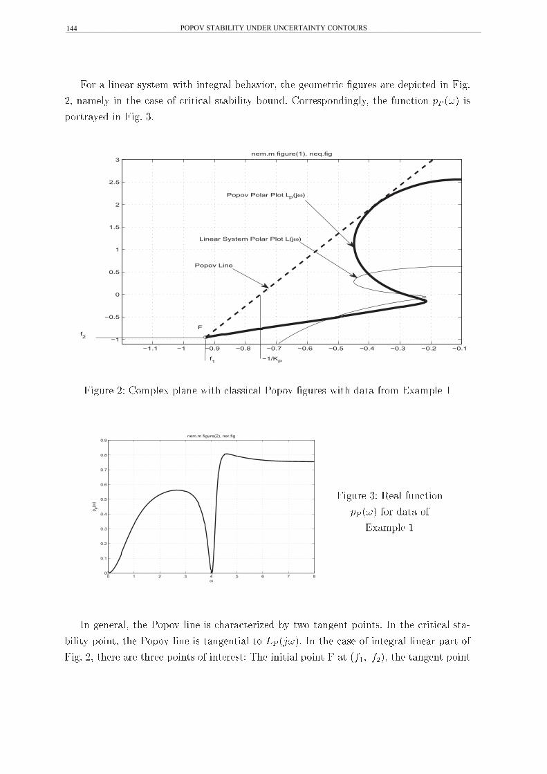
��� � ������ ��� ��� �������� ��������� ��� ��������� ����� ��� �������� �� ����
�� ����� �� ��� ��� �� �������� ������� ������ �������������� ��� �������� �� ��� �
�������� �� ���� ��
−1.1 −1 −0.9 −0.8 −0.7 −0.6 −0.5 −0.4 −0.3 −0.2 −0.1
−1
−0.5
0
0.5
1
1.5
2
2.5
3nem.m figure(1), neq.fig
−1/KPf1
f2
F
Popov Line
Linear System Polar Plot L(jω)
Popov Polar Plot LP(jω)
������ �� ������ ����� ��� ������� !���� ����� ��� ���� ���� " ����� #
0 1 2 3 4 5 6 7 80
0.1
0.2
0.3
0.4
0.5
0.6
0.7
0.8
0.9nem.m figure(2), ner.fig
ω
p P(ω)
������ �� $��� ��������
�� ��� ��� ���� ��
" ����� #
%� �������� ��� !���� ���� � ����������&�� � � � ������� ������ %� ��� �������� ��'
����� ������ ��� !���� ���� � ���������� �� �� ����� %� ��� ��� �� �������� ������ ���� ��
���� �� ����� ��� ����� ����� �� �������� (�� ������� ����� � �� ���� ���� ��� ������� �����
POPOV STABILITY UNDER UNCERTAINTY CONTOURS 144_________________________________________________________________________________________________________________

��� �� ������� �� ���� � ��� ��� ��� �
� ������
�
��
��� �� ����
����� �� ����
��
��� ����� � ��� ������
�� ������
���� ��� ����� � �
�� ��� ����� � �� ���
����� ���� ������
��� �� ������ �
��� �������
� �� ������ ��� �����
��
���� �� ����
� ����� ���� ������ ���� ������� ��� ������ ����� ��������� ������� � ���
������� � ��� � ! ��� �� � ��� �������� �� �" ��� ����������# ������� �� �� $������
%� ��� �&����� ��� � ��� ������
��� ������� �#�� �" ����� ����������� #��� ���� ��� ���� �� ��� '���( ����
���� ��� '���( ��� ��� )� ����*�� +�� ������)� ��� ��� ��� ��� ��� ���� ��
�� , -����� �" �� ���� �� ��)�����# ����� � �� ��� �����& ���� .��� �� ���
)��� "�� ��� ��� ��� /���"# � �� ����� �� ������ ��� �� � ��� � ! ��� ��
��� � ��� � ��
−9 −8 −7 −6 −5 −4 −3 −2 −1−60
−40
−20
0
20
40
60nfg.m figure(3), nfk.fig
ξ
η
κ
H
LH1
LH2 LP( j ω )
�� ��� ,0 1����&������� "�� � '���( ���� ��� ���� ��� ����
POPOV STABILITY UNDER UNCERTAINTY CONTOURS 145_________________________________________________________________________________________________________________

� ������ ���� ��� ���������� ����������
��� � ������� �� ��� ������� �� ������ � ������� ��� �� � ������ �� �� ����� � ������
��� ���Æ
����
�� ���� � �� ����� �� ��� ���� �� � ��� � ������ �� ����� � � ���� ������
� � �� � � �� �� ����� !��������� � �� � "� # ���� $� ��� � ������ �� �� ���� � �
����� ������ �� ���� � %�� �� ���� �� ��� �� &�� ��� ��� � ������ ���� � ��� ���������
��� �� %�� � ������ ������� �� ���� � ���� ��� ��� �� �� !��" �� ����'� &�� ����
&��(�� �� �� )�� � ��� ��������� ��������� �� !����� ��� �� ���� �� ���� *"� ��� ������ �
�� ���� ��(�����
−0.8 −0.6 −0.4 −0.21.2
1.4
1.6
1.8
2
2.2
ξ
η
nem.m figure(8), nfl.fig
LP ( j ω )
c
d
H
(ξs,ηs)
S
(ξc, ηc)αc
.
o
LPv ( j ω )
(ξH,ηH)
.PresumtivePopov Line LH1
������ *+ ,� ���� ������ ������ -���� �� �
������
������
��
� &�
!�� �" !."
����� �� ��� ���� �� ����� ������ �� ��� -���� �� � ���� ����� /���� %�� ������
� �0 ��� � &�� ��� ���������� � %�� ����� ��������� �� � ��� ����� ���� !�� ��"
POPOV STABILITY UNDER UNCERTAINTY CONTOURS 146_________________________________________________________________________________________________________________
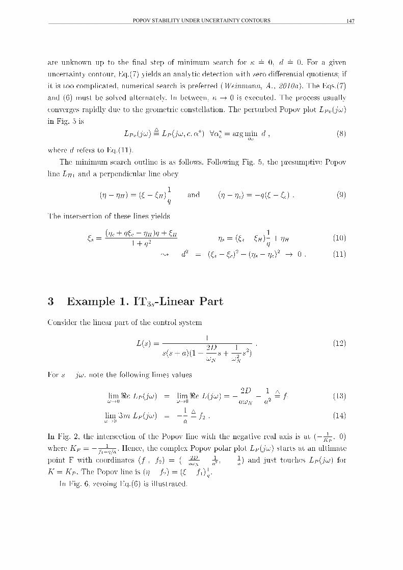
��� ������� � � �� ��� �� �� ������� ������ ��� ��� �� �
�� �� ��� � �����
��������� ������� ������ ��� � �� ��� ��� ������ ��� !��� �"������ �������# ��
� �� �� ��� ���� � �������� ������ �� ������� ���������� �� ������ $�� �������
�� �%� ��� &� �� �� � ����� �� '� &������ � � � �� �(���� � $�� ������ ���� �
��������� ��� � �� � �� �������� ����� ����� $�� ����&� )��� � �������
�� ���� * ��
��������� �� ���� ��
�� ��� � ��������
� � �+�
����� � ������ � ����,,��
$�� ������� ������ �� ��� �� �� �� ���� �� ����� ���� *� �� �������� )���
��� ��� �� � ���� ��� �� ��� �&��
� � �� � �� � ���,
��� � � �� � ���� � ��� � �-�
$�� ���������� �� ���� ���� ��� �
�� ��� . ��� � ��� . ��
, . ��� � ��� � ���
,
�. � �,��
� �� � ��� � ���� . �� � ��
�� � � �,,�
� ������� ��/ ������ ����
0���� �� �� ����� �� �� �� ����� �����
�� � �,
� . ���, .1�
�� .
,
��
�
��� �,1�
��� � ��� ��� �� �� ����� ���� �� ���
����
�� �� ���� � ����
�� ����� � �1�
����
,
���� �� �,/�
����
�� �� ���� � �,
�
�� �� � �,2�
'� ���� 1� �� ���������� �� �� )��� ��� ��� �� ������� ��� �(�� �� � �� �
�
� ��
����� �� � � �
���� �� 3����� �� ��� �( )��� � �� � �� ���� ���� � �� � ����
��� � ��� ���� ����� ���� ��� � �� ����
��
��� �
�
�� �� 4�� ������ �� ���� ���
� � �� � $�� )��� ��� �� � � ��� � �� � ����
��
'� ���� %� !������ ����%� �� � ����� �
POPOV STABILITY UNDER UNCERTAINTY CONTOURS 147_________________________________________________________________________________________________________________
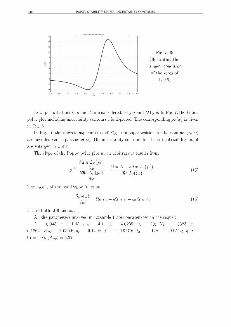
3.5 3.6 3.7 3.8 3.9 4 4.1 4.2 4.3 4.4 4.5
−4
−2
0
2
4
6
8
10
12
14
16
ω
v P(ω)
nem.m figure(3), nev.fig
������ ��
���� ���� ���
� ����� ���������
�� ��� ����� ��
������
���� ������� ����� �� � �� � �� ����������� � �� � �� � �� � � ���� � ��� !���"
�� � ��� �������� ������ ���� �������� � �� ��������� #�� ������������� �� ��� �� ��"��
�� ���� $�
� ���� %& ��� ������ ���� �������� �� ���� ' �� ������������� �� ��� ��(�� �� ���
�� ������� "����� � � (���� ��� #�� ������ ���� �������� ��� ��� ������ �� ����� �����
�� �� ���� �� ������
#�� ���� �� ��� !���" �� � ��� � � ����� �� � ������ ���(
��)
� �� ����
�� �� ����
�
)� �* �� ������
� ������� �%+�
#�� ����� �� ��� �� !���" ��������
�� ���
�) � �� � �� �� ��� �� �%��
�� ���� ���� � & �� ���
, ��� � � (����� ��"�"�� �� �- (�� % �� ���� ��� ��� �� ��� ������
� ) &�&.+/ � ) %�&+/ �� ) .�%/ �� ) .�&01$/ �� ) 0&/ �� ) %�1101/ � )
&�%$�0/ ��� ) %�&1&'/ �� ) &�%.%$/ �� ) �&�'0 '/ �� ) �%�� ) �&�'+0./ ��� )
&� ) %�&+/ ����� ) +�1 �
POPOV STABILITY UNDER UNCERTAINTY CONTOURS 148_________________________________________________________________________________________________________________

−1.1 −1 −0.9 −0.8 −0.7 −0.6 −0.5 −0.4 −0.3 −0.2 −0.1
−1
−0.5
0
0.5
1
1.5
2
2.5
3
3.5nem.m figure(4), nex.fig
Popov Line
−1/KPv
Popov Polar PlotLP(jω) Including Uncertainty
������ �� �� � �� � � ��� ����� �����������
POPOV STABILITY UNDER UNCERTAINTY CONTOURS 149_________________________________________________________________________________________________________________
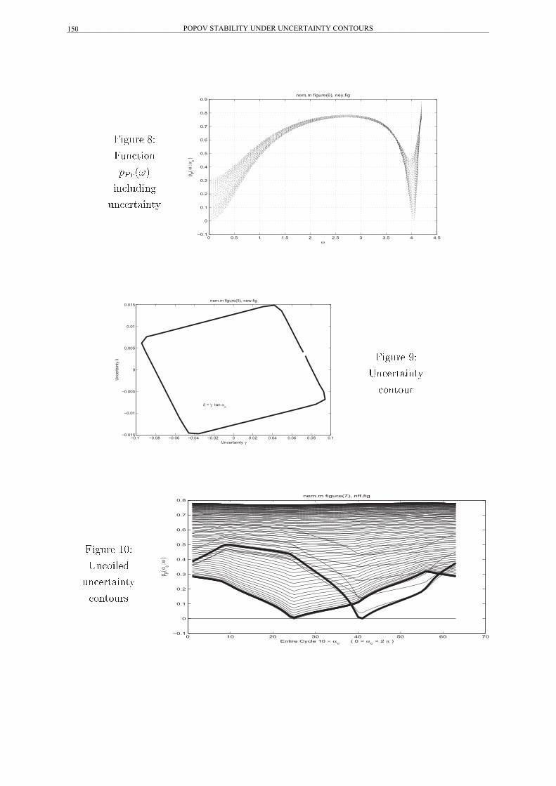
������ ��
�����
��� ��
������
��������
0 0.5 1 1.5 2 2.5 3 3.5 4 4.5−0.1
0
0.1
0.2
0.3
0.4
0.5
0.6
0.7
0.8
0.9
ω
p P(ω ; α
c )
nem.m figure(6), ney.fig
−0.1 −0.08 −0.06 −0.04 −0.02 0 0.02 0.04 0.06 0.08 0.1−0.015
−0.01
−0.005
0
0.005
0.01
0.015nem.m figure(5), new.fig
Uncertainty γ
Unce
rtaint
yδ
δ = γ tan αc
������ ��
��������
�����
������ ���
������
��������
������
0 10 20 30 40 50 60 70−0.1
0
0.1
0.2
0.3
0.4
0.5
0.6
0.7
0.8nem.m figure(7), nff.fig
Entire Cycle 10 × αc ( 0 < αc < 2 π )
p P(αc ; ω
)
POPOV STABILITY UNDER UNCERTAINTY CONTOURS 150_________________________________________________________________________________________________________________

� ������� ���� ������ ����
���� ������ � ����� ���� �� � ������� �����
���� ��
� ����
���
���
��
��
��
�
� ����
���
���
��
��
��� ����
�� �� �� ��� ������ ����� ����� ���� �� ���� � ����� �� �� �� ��� ������������
�� ��� � ������ ��� ���������� �� ��� �� ��� �������� ���� �!�� !� Æ ��� ��� ���
��� !� � "������� �� #� ��� ���� �!�� ����� ����� ���� � ��������� � �� ���
−12 −10 −8 −6 −4 −2 0 2 4 6 8 10−80
−60
−40
−20
0
20
40
60
80nfg.m figure(1), nfj.fig
ξ
η
−1/KP
Linear System Polar Plot L(jω)
Popov Polar Plot LP(jω)
Popov Line with Slope 1/qv
� �� ��$ %����� ����� ����� ����� "�� &'����� �
��� ���������� ������� � &'����� � ��� �� ( )�)*+, �� ( )�)�, ��� ( *��, ��� (
-��, ( )�)��, � ( )�)+*+, ��� ������ ������ ���� � ��� ��� ��������� ��� � (
)���-., �� ( )������
POPOV STABILITY UNDER UNCERTAINTY CONTOURS 151_________________________________________________________________________________________________________________

−12 −10 −8 −6 −4 −2 0 2 4 6 8 10−80
−60
−40
−20
0
20
40
60
80nfg.m figure(4), nfi.fig
ξ
η
Popov Line
−1/KPv
Popov Polar Plot LPv(jω)
with Uncertainties
������ �� ��� ����� ���� ��������� ����������� �������� ��� ������� �
POPOV STABILITY UNDER UNCERTAINTY CONTOURS 152_________________________________________________________________________________________________________________

0 2 4 6 8 10 12 14 16−2
0
2
4
6
8
10
12
14
16nfg.m figure(2), nfm.fig
ω
p P(ω)
������ �� ��� �� �� ��� ��� ������� �
� ���������
��� ����� ����� ���� ���� � ���������������� �� ��� ���� �� ��� � ���� !"!��� �! !������#
$� �! !������� ��� ����!� ��!����� !�������" � ��"!�! � ����� �� ���� � ��� � ����� �" ���
� � !�������" ��%������ �!# ��� �������! ��� !��� ��� ��� ���� !��� ����!������ #
����������
������ ��� �� ���������� ����� ����� ���������� ������
�� ������ ����� ��� ����������� ����� ����� ��� ���� �� ��������� ��� ��������������
�� ����� ����� ������� �
�������������� ����� ������ ��� ��� ��� � !�"�� �� ���� ������ ������ �� �� �� ��
� ������� �� ������!����� "�" #��� $%��� �� &����'
#������ ��� ����� ����� ���������(� )* + ,��� -����� ������
�� $��� #���� ����� + ������!���� �. ��� #���� �������� %&&&'(��� ������� ��* /0) /01
" )� ��#�� ��� ������ ��*�� ��+�� ����� ������ ��������� �� ����������� ��2 3�(�
��42 ����
!��$ ,��$-��� ���.� +���� �� �������� �. ������� ������ �������� �������� 5� 2�
�$/$0� 1���� ��2.� ������������ �. ������ �������� ������
�3$ ��4��� 5�� ���.� ��������� ����� ���� 66� 7* + ,��� �� ����� ����� ������� �
*�6���)��� "�� ��+.� ����� ���������( 66� - ����2���� 8��2��
1��� � ��� ����� ��� ���� ������ �� �������� ��2 3�(� 4���� �� -���
7�������� ��� 9������ � ������ .� �� �� ������ �������� � 8 �� & �9��$������9 )�� %�:$�'
����$� ������9 � �� ���
7�������� ��� �� �������� ����� �� ������� #�6������� ��� �� ��� ��� �� ���
7�������� ��� ��� ��� �� ����� ������� ���� �� � �������� ���� %��� �� �)�$��'
��$� �) ���� ��� ���� ��� �
POPOV STABILITY UNDER UNCERTAINTY CONTOURS 153_________________________________________________________________________________________________________________

������ ���� ������ ����� � �
� ���� �� � ������
��������� ������� ��� ����� ������ ����
����� �������� �� ����������� �������� �� ��������� ��� ������
!�������������� "#$"%&'#(� �$)*+* ����� & ������
,����- .+' ) /00*) '#())� 1��- .+' ) /00*) '#(%%
����- ���������������������
�������� ������� ���� ��� ����
��������
����� �� � ����� ��� � ��� �� �� ���� ��� ��� �� �� ���� �� �� � �������
��� �� ��� �� ���� �� ���� ��� �� �� ������� �� �� ���� ��� ���� �� �� ������ ��
�� ���� �� ���� �� ����� � � ���� � �� ��������� �� ��� ��� �� � �� ���� ����
�������� ���� �� �� ������� � ����� �� �� ��������� �� � ���� � ������ ���� � ��
�� ������� ������� ����� ��� �� ���� �� ����� ���� �� ����� ���
�������� ��������� ��� � ���������� �� � ��� �����
� ����������
�� ����� ������ � �� � ������ �� ������ � � � �� ��� ��� ��������� ���� �� ���
������ � �� �� � � � ���� �� � ���� ��� �� �� ������� ����� �� � ������ � ��
� � � �������������� �� ����� �� ���� � ��� � �� ����� ���� � �� � ������ � ��� �
����� ��� � �����!�� ���� �� �� ��� � � � �� �� �� �������� �� � ��� � �������
�� �� �� �� ��������� ������ � ������ � ������ �� "� ������� ���� ��� ������
� �� ����� �� �� �� ������ �� ���� ����� #���� �� � �� � ��� �� ���� �
������� ������� �� ����������� �� � ������ �� ���� � ���� ��� � ��� ����
��� � � �� � ���� $����� �� %� ������ ������� �� ����� �� ���� �� � ��� ���
��������� �� � ��������� � ���� �� ������ �� ���� ��� � �������� ������ �� ����
���������� ����� � ��������� �� ��� � �������� � &� � �� ��������� �� ���'� � ��
ROBUST CIRCLE CRITERION BASED ON AN UNCERTAINTY ENVELOPE154_________________________________________________________________________________________________________________

��������� �� ������ ��� � ������� �� � � ���������� ������� ��� �� ��� �� ����
������������ � ��� ���� �� ��� � � ��� ������� ������ ����� � � ������� ��
������������ ����� � � ����� �� � � �������� �� �������� �� ���������� ��������
� �� ���� ��� ��� � � ������� � �� ������� � � ������ ������ ���� � � ���
� � � � ������� �� � ����� �������� �� �� �� ���������� � �� ����� � � ���
�� �������� ��������� ��� �� � � �������� �� � � ��������� ������ �� ����������
�� ������� ���� ���� �� � � ������� ����������� ������������� �� � � ������� �� �
������ �������
!����� � � "���� � ����� #���� ����� � �� ��� ����� ����� ���� ������� �����
���������� �� ����� �!�"���� ��� ����� ��# � ��� $%%� $ ��� �% &�� �������� ���
������ #����� &��� '$� � � ������ ������ ��������� ���� �� �������� &�� (��� ���� ������
� � ����� ����� �� ������� �� ����� ���� ��� �� �������� &�� ��� ������ ��
� � �������� ����� � � ���� ����� �������� � � ��� ����� ���� �� �������� ����� � �
��� ���� ���� �� ����� ������ � � ��� ������
)����������� �� ���� ���� ������������ �� ���� ���� �� ����� � � ��� � �
������ ������ #�"�&����'� ��� �' ���� ����� ���(��)� ����� � *��+"� ��,�� ���-�
."�''�+"�� �� /�,�� �' ���� $%%� $ �� ���� ���� ���� ���������� ���� *������ �� ���
��� �� ����� � ���� ������ #�'"��'�� *�,�� � 0����' 1�� $%%$ $�
�� ��
� �+ �
��
��
������
�
����� ������ �
�#�$
�����
,���� -�� ��� )���������
&����� '% *������ ������ ��� ��������������� ������� � ����������
��� � �� � ��� �� ���� ��� �� � � ������ ������ ��� ����������������
����������
� ��������� ���� �����
.� �������� � � ������ �� &��� ' ��� � � ������� �������� �#�$ �� � � ���� ����
!�������� �� � � ����������� ������ �� � � ��������� ��������� � ���������� ��#��� ��$
ROBUST CIRCLE CRITERION BASED ON AN UNCERTAINTY ENVELOPE 155_________________________________________________________________________________________________________________

�� ��� ��������� � ���� ������ � ������� ����� ��� ��� �� ������ �� �� �� �� ���
��������
���
��
Æ
�� ����
�� ���� � ������� � �� � ���
��� ���� �� �� � ���� ��� �������� � ������
��� � ����������� ���
����������
�� ����� ���
�������� ���� ! �� ��� ������ ��� ������ ��
���
��
Æ
�� � � ��"�� ������
�� #� Æ � Æ�"�� �� ����� #� �$�
��� ��������� � ���� ������ ����
��� � �������� ��� ��� � ��� � �
����"��� ����#� ��� �� �
�����
��� �
� �%�
�����
�� ������ ��� �&�
'�� ������ ���� �� ��� ������(������ � ������ �
������ �������� ��� �)�
��� ��� � � �� � ������ �����
��� ��
� ��� � �*�
��� + �� �� '�� ��������� � ����������� �� � ���� ���� ���� ��
,����� �� �� ��� ������ � ��� ��� !���� �� � �� ��� ��� !����-��!� ����������
������
��
��� �� � � � �
�
��� �� � � � �.�
��� ���
�� � �� ���
��� � � ��/�
��� � ������0 ��!��� ��� ����� ������ ��� ��� ���� �� ��!�� �(����� ������ 1� ����� ��
��� � � ����� ������ ��� � ����� ��� � ����� ��� ����� ��� �� ���� �� � � ��(�
� �������� �� � ����� �� ��� � ���������� �
2���� �� 3�'4�2 ������� ������ ��� �� 5���&� � ������ ���� '�� ����� � ��� ����
� + �� �� 1� �������� ��� ���������� ���� �� ��� ������ �� �� � ���!��
ROBUST CIRCLE CRITERION BASED ON AN UNCERTAINTY ENVELOPE156_________________________________________________________________________________________________________________
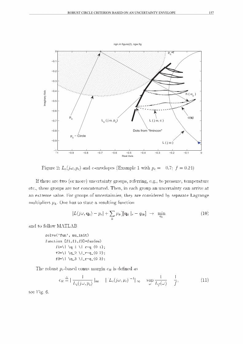
−1 −0.9 −0.8 −0.7 −0.6 −0.5 −0.4 −0.3 −0.2 −0.1 0−1
−0.9
−0.8
−0.7
−0.6
−0.5
−0.4
−0.3
−0.2
−0.1
0
ngn.m figure(2), ngw.fig
Real Axis
Imag
inar
y Ax
is
pc
pc − Circle
pc+f
h ( αc )
Dots from "fmincon"
c(q)
L ( j ω )
L ( j ω, c )Lc ( j ω, pc)
������ �� ����� �� �� ����������� ������� � ���� �� � ����� � � ����
! ����� ��� ��� �� ���� ��"�������# ������$ ��!������$ �%�%$ �� ��������$ �����������
��"%$ ����� ������ ��� ��� "��"������� % &���$ �� ��"� ����� �� ��"�������# "�� ������ ��
�� ������� �����% ��� ������ �! ��"����������$ ���# ��� "���� ��� '# �������� (�������
����������� �% )�� ��� �� ����� � ��������� !��"����
�������� ���*�
�
�+����� � ��, � �����
��
�� �� !����� -.&(./
���������� � ����
����� ���������������
����� �� � �� ��� �� ���
� ��� �� �� ��� �� ��
����� �� � �� ��� �� ���
&�� ��'��� ���'��� "���� ������ �� �� �0�� ��
���� �
�
����� ���� � �+����� ��,
���� � ����
�
�� ��
�
�� ��
��� ���% 1%
ROBUST CIRCLE CRITERION BASED ON AN UNCERTAINTY ENVELOPE 157_________________________________________________________________________________________________________________

������������ � �� ����� � �������� ��� ����� ��� ��� � ���� ����� �����
�������� ������ ����� ������ ������� �� ��������� ��������� �������� ���� ��
� � ������ ��� ������������� �� ������ � � � ������ ��� ����� � �� �������
���� ���� ! �� "����� #�
� ������� �� ��� ��$��������
% � "����� �� ��������� �� ���� �� ������� ���� �� � � ���� � ������
���# &
���' �#� '(�
��
�'
��
�
��#� (#
��� � & )* � & !!+,* � & !,* �� & + * �� & �!)�
% � �������� � �� � ��������� �� ��� ��� � ��� �� & ! �� & !! ,� % �
������� ������ �� ���� $ �� � & !()-! � �� & $- �
% � ���� $ ������ � � ��������� �������� ���������� .� ����� + �� ,� � � �
��������� �������� ����� ��# �� � � ������� �� � ���� ��� ������ ����������� ��
�� ����� �� ��� ��� ��� �� � �� ��� � � � ���������� ��� ����� ��# �� ����������
��������� �� ���� ,� �������� � � ����������� % � ������� �� �� �� ����� �� ���� /�
−1 −0.8 −0.6 −0.4 −0.2 0 0.2 0.4 0.6 0.8 1−1
−0.5
0
0.5
1nfx.m figure(1), nfz.fig
γ
δ
0 10 20 30 40 50 60 70 80 90 100−1
−0.5
0
0.5
1
αc
γ
0 10 20 30 40 50 60 70 80 90 100−1
−0.5
0
0.5
1
αc
δ
������ $� 0�������� �� !! ������
ROBUST CIRCLE CRITERION BASED ON AN UNCERTAINTY ENVELOPE158_________________________________________________________________________________________________________________

−0.8 −0.6 −0.4 −0.2 0 0.2−1
−0.8
−0.6
−0.4
−0.2
0
0.2
0.4
0.6
0.8
1nfx.m figure(2), nfy.fig
pc
pc−Circle
L ( j ω, c )
L ( j ω )
Lc ( j ω, pc )
������ �� ���� ���� �� ����� �� ��� ��� ����� ����� ���� �� ����� ��� ��� ���������
���� � ���� � �� �� ��� ���������� ��� �� � ������������ �� ���� � ��!�������
���� ���� ����� �� ����� ���
������� � ����!� �� �� � ��� ������ ����!� ��� "��#��� ������ � ����� ��
������ � ���������� �� ���� $% �!��� ����� � � !���!�! � ��� ���&������� ����� �
�% ����� ��� ����������� ��� � !���!�! ����� � ���&����# �� ��� � ��' � �( ��!�
��� �&���� )�� ����!� �� �������� � � �� �!���# ����� �*�� �#� �!% ��� ���� ���
ROBUST CIRCLE CRITERION BASED ON AN UNCERTAINTY ENVELOPE 159_________________________________________________________________________________________________________________

−1 −0.8 −0.6 −0.4 −0.2 0 0.2−1
−0.8
−0.6
−0.4
−0.2
0
0.2
0.4
0.6
0.8
1nfx.m figure(3), nga.fig
pc−Circle
−1/KP1
pc
−1/KP2
Lc ( j ω, pc )
������ �� ������� ���� ����� ������ ��� ��� ��� �� ��
������ ��
�������
�� ��� ���
����� ����
������ ��
����� � ��
���� �����
���
0 0.5 1 1.5 2 2.5 3 3.5 4 4.5 50
0.5
1
1.5
2
2.5
3
3.5nfx.m figure(4), nha.fig
ω
1/Lf(ω)
Peak Height 1 / f
ωs
ROBUST CIRCLE CRITERION BASED ON AN UNCERTAINTY ENVELOPE160_________________________________________________________________________________________________________________

−1.1 −1 −0.9 −0.8 −0.7 −0.6 −0.5 −0.4 −0.3 −0.2
−0.6
−0.5
−0.4
−0.3
−0.2
−0.1
0
0.1
0.2
0.3
0.4nfx1.m figure(3), nhl.fig
Lc ( j ω, pc )pc − Circles
������ �� � �� ��� ���������� ��� �� � �����������
−1.1 −1 −0.9 −0.8 −0.7 −0.6 −0.5 −0.40
0.5
1
1.5
2
2.5
3nfx1.m figure(4), nhm.fig
pc
fKP2
KP1
������ ��
����������
����� �����
���� �����
ROBUST CIRCLE CRITERION BASED ON AN UNCERTAINTY ENVELOPE 161_________________________________________________________________________________________________________________

0 0.5 1 1.5 2 2.5 3 3.5 4 4.5 50
0.5
1
1.5
2
2.5
3
3.5
4
4.5
5nfx2.m figure(4), nhu.fig
ω
1/Lf(ω
) a=0.68 ������ ��
����� ��
������ �
0.4 0.5 0.6 0.7 0.8 0.9 1 1.1 1.20.2
0.4
0.6
0.8
1
1.2
a
nfx2.m figure(5), nht.fig
f = minω Lf
Conus (KP2−KP1)
������ ��
����� ��
��� ���������
�������� � �
�����������
��� ������
������
ROBUST CIRCLE CRITERION BASED ON AN UNCERTAINTY ENVELOPE162_________________________________________________________________________________________________________________

� ������� �� ��� ������ ���� �� ����� �� ����
������
��� ������� ���� � ��� � ��� ������ ���� ��
���� � ������� � ������ � ������ ���
����� � �� � ����� � ������
���� � ��� ��� ��� � �� ��������� �� ������� �������� ��� ������ � ������� �����!��"
��������#��$%
& � � � �" ��� ������ �� ���'� � �$���( � ��� ��� � ����� �� �������� �
� !��������!!� � ��������% )����� ���*����$ �� +�#�� � ��� �� ���+ �����(�����
��� �� � � �, ���� -�(����$ � ( �.�%���% � � �.�%!��%�� ���� &�+% ���%
��� ����(���� ����� �� ��� �(���� � /0%���� �� �����*�� *$ ��� ��� ��� ��'
��(���� � �� ��� ��� (���� � *$ ��Æ" ����� �� � ���� �� � ���� �� � ����%
��� )����� *���� ���*����$ ���� � �� �% � � �%��% & �� ���+ ��� ������ ��� ��( ���� �
���������$" ��� ���*����$ ���� � �� �� � �� � � �� � ���" ���+���$ �(����� ���� ���
)����� ���� �% ��� ���*����$ ���+� ����� ���� ���������$" �%�%" ��� ��(����*�� ���� � �
��� �����*�� �$���(" �� �� � ������ � �� � �����! ���� &�+% ���% ��� (���((
�������� �� � ������ �� �� � ����%
&�+�� ��, 1 � � �� �
���� � � �����������������������
�����������������
−2 −1 0 1 2 3 4 5
−8
−6
−4
−2
0
2
4
6
8
ngb.m figure(3), ngr.fig
Real Axis
Imag
inar
y A
xis
V=4
ROBUST CIRCLE CRITERION BASED ON AN UNCERTAINTY ENVELOPE 163_________________________________________________________________________________________________________________

−2.2 −2 −1.8 −1.6 −1.4 −1.2 −1 −0.8 −0.6−1
−0.8
−0.6
−0.4
−0.2
0
0.2
0.4
0.6
0.8
1
ngc.m figure(2), ngs.fig
Real Axis
Ima
gin
ary
Axis
Lc ( j ω, pc )pc
L ( j ω )
L ( j ω, c )
������ �� ������� �������� ����� ���� ��� � � � ���� ���������� ��� �� � �
ROBUST CIRCLE CRITERION BASED ON AN UNCERTAINTY ENVELOPE164_________________________________________________________________________________________________________________

� ������� �� ��� ����������
��� ����� �� ��
� �� ����
�� �� �� ��� ���
��� ������� � ��� � �� ������ �� ��� ��� ��� ����������� ��� ��� � �� � �
���� � � ���� �� � � �� � !�� �� � "�� � � ����
−0.2 0 0.2 0.4 0.6 0.8 1
−0.6
−0.5
−0.4
−0.3
−0.2
−0.1
0
nfp1.m figure(2), ngu.fig
pcL ( j ω )
Lc ( j ω, pc )
pc − circle
#�$�� ��% &'�� �'�� (' )*���� �
#'� #�$� �� '�� +��� ��� �,����� ����� � ��"��-� �� � �"�� �� ��� �� �
����!� ������� ��� � ��!���� ��� � ���- -��
ROBUST CIRCLE CRITERION BASED ON AN UNCERTAINTY ENVELOPE 165_________________________________________________________________________________________________________________

� ������� �� ��� ���������� � � ��������� ����
���� ������
������� ��� ��� �� �� ��� ����� ������ �� ��� ����������
���� ��� � ��
�� �� � �� ��� � �� �� � � � ����
����
��� �� �������
�� � � � � � ����
�� �� �������
�� � � Æ � � � ����
�����! �� "#$�%� �� &�!$ '(
������� � �� )������ �*�
� � ��� )�����*�� � ��+�
,����� �� � � � �+- � � '- � � ���.�- � � %$
"/�� ����!� ���� �� /�� ���� � �0�� �( ��� �������� ������� �� ������1�� ��
��/� ��2�������2�0��� �� ������ �� ��3������- ����( ��� ���/��/� ���������
�����
������ ����( ��� &�!�$ ��( ��( �.$
&� ���� ��4���� �� � �%� + ���( ����� ����� � ����� �� ��� ��#�� $
5�/� ��4���� �� ������� ����� / ��� � �#���� �� �� /��! ���������
���� �$
&� ��!��/� / ��� �� �� Æ( ��� "#$��.�$ &�� �( ��� ���� � �� � �� ���
���� ���� ���$
��� 3!� �� �� �� � � �� ����� �� ��� �� ����/� � ���������� ���� � �� ���
����������� �� Æ /���� ��$ ��� �������� �� � ���� �� ��4������ � �����/� ������
� � �� ���������� � Æ � � � ��������
�� � ��.�
ROBUST CIRCLE CRITERION BASED ON AN UNCERTAINTY ENVELOPE166_________________________________________________________________________________________________________________

0 1 2 3 4 5 6 7−4
−3
−2
−1
0
1
2
3
4
5
6nhe.m figure(1), nhi4.fig
αc
d |h|2 / d αc|h|γδ
| Lc ( j ω, pc) |
������ �� ��� ��� �������� ������� ��� ��� ���������� �� ��� ������ ���� ������� �� ��
��� � � � � �������� ��� �� � �
−2 −1 0 1 2 3 4−5
−4.5
−4
−3.5
−3
−2.5
−2
−1.5
−1
−0.5
0
nhe.m figure(2) Nyquist Diagramm, nhj4.fig
Real Axis
Imagina
ry Axis
h ( αc )
pc
| Lc ( j ω, pc ) |
L ( j ω )
������ �� ����� ������ ������ �������� ��� ����������� ���� ��� �� � �
ROBUST CIRCLE CRITERION BASED ON AN UNCERTAINTY ENVELOPE 167_________________________________________________________________________________________________________________

0 1 2 3 4 5 6 7−4
−3
−2
−1
0
1
2
3
4
5
6nhe.m figure(1), nhi8.fig
αc
d |h|2 / d αc|h|γδ
| Lc ( j ω, pc) |
������ �� ��� ��� �������� ������� ��� ��� ���������� �� ��� ������ ���� ������� �� ��
��� � � � � �������� ��� ��� �� � �
−2 −1 0 1 2 3 4−5
−4.5
−4
−3.5
−3
−2.5
−2
−1.5
−1
−0.5
0
nhe.m figure(2) Nyquist Diagramm, nhj8.fig
Real Axis
Imagina
ry Axis
h ( αc )
pc
| Lc ( j ω, pc ) |
L ( j ω )
������ �� ������������� !���� ������"" ��� ����������! �� # ��� �� � �
ROBUST CIRCLE CRITERION BASED ON AN UNCERTAINTY ENVELOPE168_________________________________________________________________________________________________________________

0 1 2 3 4 5 6 7−4
−3
−2
−1
0
1
2
3
4
5
6nhe.m figure(1), nhi16.fig
αc
d |h|2 / d αc|h|γδ
| Lc ( j ω, pc) |
������ �� ��� ��� �������� ������� ��� ��� ���������� �� ��� ������ ���� ������� �� ��
��� � � � � �������� ��� �� � ��
−2 −1 0 1 2 3 4−5
−4.5
−4
−3.5
−3
−2.5
−2
−1.5
−1
−0.5
0
nhe.m figure(2) Nyquist Diagramm, nhj16.fig
Real Axis
Imagina
ry Axis
h ( αc )
pc| Lc ( j ω, pc ) |
L ( j ω )
������ �� ������������� !���� ������"" ��� ����������! �� # ��� �� � ��
ROBUST CIRCLE CRITERION BASED ON AN UNCERTAINTY ENVELOPE 169_________________________________________________________________________________________________________________

����� ��� �� �
�� � � � ������������������ � � �����������������
�� � � ������������������ � ��������
� ������ � � ��������������������� � � ������������������ � �������
������ ������ ��� �! �� " �
������������������������� #�������������� � � �����������������
�� � � ������������������ � �������
���� � � � ������������������ � � �����������������
�� � � ������������������ � ������
������������������� #�������������� � � �����������������
�� � � ������������������ � �����
����������������������������� #��� � � �����������������
�� � � ������������������ � �����
� ������������������������������� #��� � � ����������������
�� � � ������������������� �� � � ������������������ � ��������
� $����������������������������������� #��� � � ������������������
�� � � ����������������� �� � � ������������������ � �������
� ���������
��� ����������� ������ ����� ���� ��� ��� ������ ����� ������ ���� ���� �����������
��� ��� �������� �������� �� �������� �������� ����������� ��������� �������������� ��
��� ���������� �������� ��� ������� ��� �� ������� ��� ����������� ������ ����� ����
����� ��� ���� �� ���� �� ��������� ��� ������ �������� � ��� ������ � ���� ���� ����������
������������� ���� ������������� �������� ��� ������ �� ������������ ��� ��������
����������
������ ��� �� ���������� ����� ����� ���������� ������
�� ������ ����� ��� ������ ���� � ��� ���� �� �������� �� ������� ������� �������
���� ��� ��� ������ �� ��� ����� ������ ����� ���� ���� ���� ��� ���� ���!
� ����� ������ ����� ������ ��� ��� ��!� "�#�� �� "��� ������ ������ �� �� �� ��
� ������� �� #�����$����� %�% &��� '���� �� (����)
� �$�!!��� #�� �� !� � %�� ��� � ����� ������ ����� ����� #� �� �� ������� �������� ��
����*� ������ �������� ����&������ ���� ��� !+ ,-
������� %�� ���'� ����� ���������.� �� / 0��� 1����� ������
#��� ����� ��� %����� ��(�� ��)*� 2���� ������ ��������� �� ����������� 2�3� ����
%��+��,� #���� ��� �-��� � ����� ����� /���� �� �������� �� ������� ���� ������ ���
����� �� ������� ������.� ����&������ �� � ��� ,,� ,,�
.�-������ ��� �� &���* �������� ��� �������� ����� �� ���� �� �������-�� �����-�
��� ���� ��� �
ROBUST CIRCLE CRITERION BASED ON AN UNCERTAINTY ENVELOPE170_________________________________________________________________________________________________________________

Report IFAC Workshop
Supplemental Ways for Improving International Stability Bucharest, Romania
October 28 – 30, 2009 Supplemental Ways for Improving International Stability - SWIIS - has a long tradition in IFAC. According to the triennial cycle after Prishtina (Kosovo) 2006 the Workshop was organised this year by the Faculty of "Control and Computers" of the "University Politechnica of Bucharest" from October 28 to 30, 2009 in Bucharest, Romania. The program included 3 plenary papers, 18 technical papers and 2 panel discussions. The plenary papers dealt with a new approach for simulation of sociotechnical systems, international stability issues and globalisation. According to the scope of SWIIS the topics of the technical papers were heterogenous. One block of papers dealt with complex - adaptive - systems. Such systems are more and more introduced not only for modelling and control of socioeconomic systems. Another session was about software piracy, existing laws and the impact to economy. Cooperative networks offer the possibility to design an umbrella for different applications. Further topics adressed were fuzzy methods, ethics in IT, collaborative software platforms, ……. The two survey papers by F. Kile "Improving Policy Choices through Simulation" and G. Dimirovski " International Stability Issues: Individual vs. Collaborative behaviours in Complex Dynamical Networks by Controlled Synchronisation" gave an excellent overview on these subjects. In the panel discussion " Impact of the crisis on Social Stability" was mentioned that in terms of SWIIS the problem could be seen as a stability problem of a very complex system. To solve this problem new theoretical approaches are necessary. The other panel discussion "Education and Research in a Global Society" was naturally concentrated to Universities. 42 participants attended the very well organised event. The next Workshop will take place in Prishtina, Kosovo, October 27 – 29, 2010 and is organised by the local IFAC NMO. P. Kopacek
REPORT IFAC WORKSHOP SUPPLEMENTAL WAYS FOR IMPROVING INTERNATIONAL STABILITY 171_________________________________________________________________________________________________________________
Kooperationsworkshop über menschenähnliche Roboter
TU Wien, 26 Jänner 2010
Im Rahmen der Kooperationsabkommen der TU Wien mit der University of Manitoba ( Kanada) und der National Kaohsiung First University of Science and Technology (NKFUST),Taiwan, R.O.C, fand am 26. Jänner 2010 an der TU Wien eines der ersten internationalen, wissenschaftlichen Workshops über humanoide Roboter in Österreich statt. Wie in der, vor kurzen fertiggstellten, BMVIT Studie „ Robtics in Austria“ ausgeführt liegen in Österreich, von der theoretischen Seite, Potenziale brach welche unmittelbar auf diese moderne Technologie angewandt werden können. Hauptzweck dieser Veranstaltung war es daher österreichischen Universitäts- und Forschungsinstituten sowie der einschlägigen Industrie einen tieferen Einblick in die theoretischen Hintergründe dieses rapid wachsenden Marktes zu geben. Der Schwerpunkt lag dabei auf, menschenähnlichen, intelligenten, mobilen Robotern sowie auf dreidimensionalen „ Sehen“. P. Kopacek berichtete über den Stand der Robotertechnik in Österreich und ergänzte seine Ausführungen. durch Beispiele ausgeführter Projekte. Sodann stellten B. McKinnon, J. Baltes und J. Anderson von der Universität Manitoba ein neues Verfahren für dreidimensionales Sehen basierend auf der Liniensegmenterkennung vor. Fuzzy Methoden haben an der NKFUST eine lange Tradition. K.Y. Tu beschäftigte sich in seinem Vortrag mit der Anwendung dieser Methode zum „Robusten Gehen“ humanoider Roboter. Anschließend gab P. Kopacek einen Überblick über Forschungsarbeiten auf dem Gebiet der autonomen, mobilen Roboter an der TU Wien. Wettkämpfe humanoider Roboter werden immer beliebter. J. Baltes und J. Anderson gaben daher im nächsten Vortrag einen Überblick über diese „Sportdisziplinen“. Ein neuer an der NKFUST entwickelter Roboter (NeiDau) mit Kraft- und Momenten Sensoren wurde von K. Y Tu vorgestellt. Über das Gemeinschaftsprojekt „Humanioder Roboter Archie“ referierten J. Baltes und P. Kopacek. Den Abschluss bildete ein Vortrag von Y. T. Yang von der Tamkang Universität in Taiwan über das emotionelle Verhalten von Spielzeugrobotern. Laut übereinstimmender Meinung der ungefähr 50 Teilnehmer erfüllte diese Veranstaltung ihren Zweck einen Einblick in Arbeiten aus Österreich, Kanada und Taiwan zu geben um zukünftige, kooperative Forschungsprojekte zu initialisieren. und der Roboterforschung in Österreich weitere Impulse zu verleihen. Die Bedeutung der Veranstaltung wurde dadurch unterstrichen, daß diese vom Botschafter Taiwans, dem Handelsrat Kanadas und seitens der TU Wien, von Vizerektor H. Kaiser eröffnet wurde. P.Kopacek
KOOPERATIONSWORKSHOP ÜBER MENSCHENÄHNLICHE ROBOTER172_________________________________________________________________________________________________________________

Bausteine mechatronischer Systeme
W. Bolton
3. Auflage, Pearson Studium, 2006 ISBN 3-8273-7098-1
Die Integration der verschiedenen Ingenieurwissenschaften in Studium und Beruf wird immer wichtiger. Dieses interdisziplinär ausgerichtete Lehrbuch zu den Bausteinen mechatronischer Systeme vermittelt daher die wichtigsten Kenntnisse aus der Elektrotechnik, des Maschinenbaus und der Informatik, um mechatronische Systeme in der Theorie und in der späteren Berufspraxis zu verstehen. Der Leser lernt an vielen Beispielen mit Übungsaufgaben und Lösungen, wie sich die Verzahnung der Teilgebiete in der Mechatronik gestaltet. Zugleich ermöglicht dieser Blick über den Tellerrand, dass Mechatronik-Studenten mit Kollegen aus den anderen Fachgebieten problemlos kommunizieren können. Diese ganzheitliche Sichtweise hilft Studierenden, mechatronische Systeme, wie sie in der Industriepraxis üblich sind, zu verstehen und eigenständig zu entwerfen. Es werden sowohl grundlegende Systemelemente, Antriebssysteme, Systemmodelle, Microprozessorsysteme behandelt. Den Abschluss bilden zeitgemäße Beispiele mechatronischer Systeme Das Buch kann sowohl Studenten der Ingenieurwissenschaften als auch den in der Praxis stehenden wärmstens empfohlen werden. P. Kopacek
BUCHBESPRECHUNGEN 173_________________________________________________________________________________________________________________

Moderne Regelungssysteme
Richard C. Dorf und Robert H. Bishop,
10. überarbeitete Auflage, Pearson Studium, 2007 ISBN 3-8273-7162-7
Einer der Klassiker unter den Lehrbüchern über Einführung in die Regelungstechnik liegt nun in der 10. überarbeiteten deutschen Auflage vor. Wie bereits die vorghehenden englischen und deutschen Auflagen bietet es den Lesern in anschaulicher Form einen ersten Einblick in die moderne Regelungstechnik. Dies wird dadurch erreicht, dass die Verfahren und Methoden durch anschauliche Beispiele erläutert werden. Dadurch erkennt der Leser sehr schnell die kaum überschaubare Vielfalt moderner regelungstechnischer Anwendungen, wodurch sein Interesse am Fach Regelungstechnik geweckt wird. Ziel des Buches ist es, die Grundlagen des Entwurfs von Regelungssystemen im Zeit- und Frequenzbereich in klarer und anschaulicher Weise darzustellen. Der Bogen erstreckt sich dabei über Verfahren der klassischen Regelungstechnik bis hin zu Zustandsraumverfahren. Darüber hinaus werden auch die neuesten Entwicklungen der Regelungstechnik, wie beispielsweise robuste Regelungssysteme, Anwendung computerunterstützter digitaler Regelungssysteme, … behandelt. Am Ende jedes Kapitels befindet sich ein Abschnitt über MAT-LAB in dem der Lernende mit den Grundlagen der rechnergestützen Synthese und Analyse von Regelungssystemen vertraut gemacht werden soll. Das Buch kann sowohl Studenten der Ingenieurwissenschaften als auch den in der Praxis stehenden wärmstens empfohlen werden. P. Kopacek
BUCHBESPRECHUNGEN174_________________________________________________________________________________________________________________

Instruction to authors – presented as a pattern paper (18 pt)
A. Maier, F. Huber (12 pt) Department ....., Vienna, Austria
Received April 8, 1999
Abstract This paper shows …… (italics, 12 pt) 1 General (14 pt) Authors should prepare their manuscript camera ready, format A 4, 12 typeface and must present their manuscript in good quality. At the left/right edge 2.5 cm, at the to/bottom edge 3 cm. Authors are invited to use papers of this journal as a sample. Please do not use an eraser or erasing fluid. Footnotes should be avoided if possible. Authors are expected to submit their paper to one of the publishers (O.Univ.Prof.Dr. Peter Kopacek, Intelligent Handling Devices and Robotics, Vienna University of Technology, Favoritenstrasse 9-11, A-1040 Vienna, Austria, Fax: +43 1 58801-31899 or O.Univ.Prof.Dr. Alexander Weinmann, Institute of Automation and Control, Vienna University of Technology, Gusshausstr. 27-29, A-1040 Vienna, Austria, Fax: +43 1 58801 37699). Email address for submitting pdf-manuscripts: [email protected] 2 References (14 pt) Within the paper references should appear in the following form: (Mayer, H., 1990) or (Mayer, H., 1990) (12 pt); Mayer, H., 1990, discovered that.... 3 Figures and Tables (14 pt) Figures and Tables should be integrated in the paper and have to be referred to as Fig. 4.1 or Tab. 5.2. 4 References References are to be listed alphabetically according to first author. (11 pt) 5 Word Processing System/Editor Microsoft Word for Windows 1.1 or higher; Microsoft Word 5.0; TeX or LaTeX.

Wenn unzustellbar, retour an: IFAC-Beirat Österreich (E318 / E376) Favoritenstraße 9-11, A-1040 Wien / Gußhausstraße 27-29, A-1040 Wien