lempel–ziv–welch (lzw) universal lossless data compression algorithmlossless data...
TRANSCRIPT

Lempel–Ziv–Welch (LZW)
• Universal lossless data compression algorithm
• Created by Abraham Lempel, Jacob Ziv, and Terry Welch.
• It was published by Welch in 1984 as an improved implementation of
the LZ78 algorithm published by Lempel and Ziv in 1978.
• The algorithm is designed to be fast to implement but is not usually
optimal because it performs only limited analysis of the data.
Fixed Length: LZW Coding
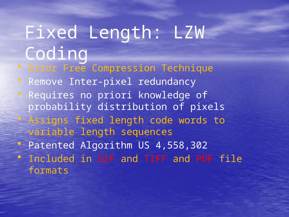
• Error Free Compression Technique• Remove Inter-pixel redundancy• Requires no priori knowledge of probability
distribution of pixels• Assigns fixed length code words to variable
length sequences• Patented Algorithm US 4,558,302• Included in GIF and TIFF and PDF file formats

• The scenario described in Welch's 1984 paper[1] encodes sequences of 8-
bit data as fixed-length 12-bit codes.
• The codes from 0 to 255 represent 1-character sequences consisting of
the corresponding 8-bit character, and the codes 256 through 4095 are created in a dictionary for sequences encountered in the data as it is encoded.
• At each stage in compression, input bytes are gathered into a sequence
until the next character would make a sequence for which there is no code yet in the dictionary.
• The code for the sequence (without that character) is emitted, and a new
code (for the sequence with that character) is added to the dictionary.

LZW Coding
• Coding Technique– A codebook or a dictionary has to be constructed
– For an 8-bit monochrome image, the first 256 entries are assigned to the gray levels 0,1,2,..,255.
– As the encoder examines image pixels, gray level sequences that are not in the dictionary are assigned to a new entry.
– For instance sequence 255-255 can be assigned to entry 256, the address following the locations reserved for gray levels 0 to 255.

LZW Coding
• Example
Consider the following 4 x 4 8 bit image
39 39 126 12639 39 126 12639 39 126 12639 39 126 126
Dictionary Location Entry
0 01 1. .255 255256 -
511 -
Initial Dictionary
LZW Coding
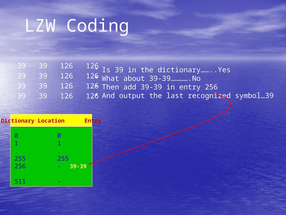
39 39 126 12639 39 126 12639 39 126 12639 39 126 126
• Is 39 in the dictionary……..Yes• What about 39-39………….No• Then add 39-39 in entry 256• And output the last recognized symbol…39
Dictionary Location Entry
0 01 1. .255 255256 -
511 -
39-39

Software Research
Workshop
• Code the following image using LZW codes
39 39 126 12639 39 126 12639 39 126 12639 39 126 126
* How can we decode the compressed sequence to obtain the original image ?

LZW Coding

Vector Quantization: Definitions
X={x1,x2,…,xN } is set of input vectors in d-D space
c={c1,c2,…,cM} is set of code vectors in the space
P is a partition of the space into M code cells (cluster) C={C1,C2,…,CM}

Structure of vector quantizer
• Code cells (clusters) are non-overlapping regions so
that the input space is completely covered.• A codevector cj is assigned to each code cell
(cluster) Cj.
• Vector quantization maps each input vector xi in
code cell
(cluster) Cj to the code vector: xi cj
• Set of code vectors is codebook

Encoding/Decoding with codebook
ImageImage CodebookCodebook CodebookCodebook ImageImagexi
jxiCj
cj
cj
xi
2),( jiji cxcxd
Distortion measure:

Distortion with measure L2
M
j Cxji
ji
cxXD1
2)(
ji Cx
jij cxCXD2
),(
• Distortion (quantization error) D for a cluster Cj:
• Distortion D for data X:
)(min}{
min XDDjc
• Optimal partition:
The optimal partition into clusters
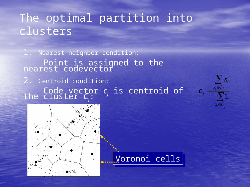
1. Nearest neighbor condition:
Point is assigned to the nearest codevector 2. Centroid condition: Code vector cj is centroid of the cluster Cj:
Voronoi cellsVoronoi cells
ji
ji
Cx
Cxi
j
x
c1

Code book generation
• Random code book
• GLA, LBG, k-means, c-means algorithm
• Merge approach: Pairwise Nearest Neighbor method
• Split approach
• Split-and-Merge approach
• Stochastic Relaxation, simulated annealing
• Genetic algorithm
• Stuctured quantizers
• Lattice quantizers

GLA: Generalized Lloyd algorithm
• Other names: LBG, k-means, or c-mean algorithm
GLA (X,P,C): returns (P,C)REPEAT FOR i:=1 TO N DO // For each point xi
j Find_Nearest_Centroid(xi,C)
FOR j:=1 TO M DO // For each cluster Cj
cj Calculate_Centroid(X,Cj)UNTIL no improvement.
C P C P
Complexity of GLA
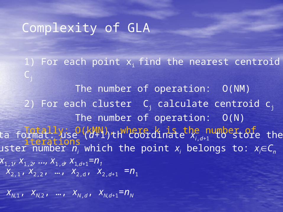
1) For each point xi find the nearest centroid Cj
The number of operation: O(NM)
2) For each cluster Cj calculate centroid cj
The number of operation: O(N)Totally: O(kMN), where k is the number of iterations
Data format: use (d+1)th coordinate xi,d+1 to store the cluster number ni which the point xi belongs to: xiCn
x1: x1,1, x1,2, …, x1,d, x1,d+1=n1
x2: x2,1, x2,2, …, x2,d, x2,d+1 =n1
…xN: xN,1, xN,2, …, xN,d, xN,d+1=nN

Wavelet transform: wavelet mother function
s
t
sts
1)(,
Translation () and dilation (scaling, s)Translation () and dilation (scaling, s)
How to obtain a set of wavelet functions?

Scaling (stretching or compressing)
s=1
s=0.5
s=0.25

Translation (shift)
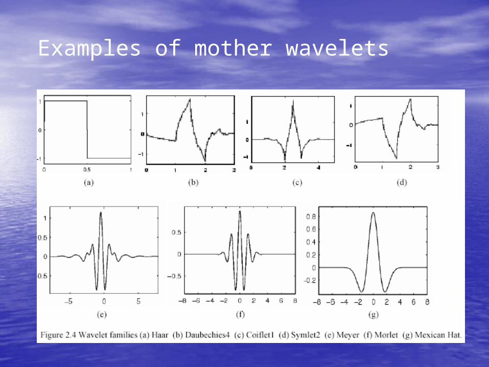
Examples of mother wavelets
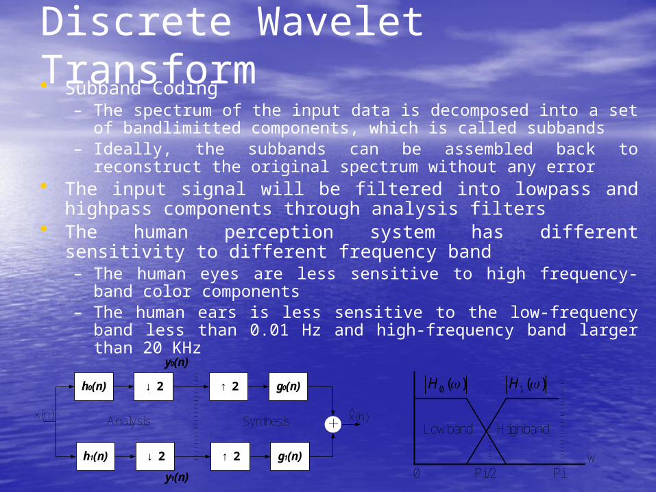
Discrete Wavelet Transform • Subband Coding
– The spectrum of the input data is decomposed into a set of bandlimitted components, which is called subbands
– Ideally, the subbands can be assembled back to reconstruct the original spectrum without any error
• The input signal will be filtered into lowpass and highpass components through analysis filters
• The human perception system has different sensitivity to different frequency band– The human eyes are less sensitive to high frequency-band color
components– The human ears is less sensitive to the low-frequency band less
than 0.01 Hz and high-frequency band larger than 20 KHz
h0(n)
h1(n)
↓ 2
↓ 2
↑ 2
↑ 2
g0(n)
g1(n)
+Analysis Synthesis
-----------------------
x(n) x(n)^
y0(n)
y1(n)
0 ( )H 1( )H
0 Pi/2 Pi
-----------------------
---------
Lowband Highband
w

Subband Transform• Separate the high freq. and the low freq. by
subband decomposition

Subband Transform• Filter each row and downsample the filter output to obtain two
N x M/2 images.• Filter each column and downsample the filter output to obtain
four N/2 x M/2 images

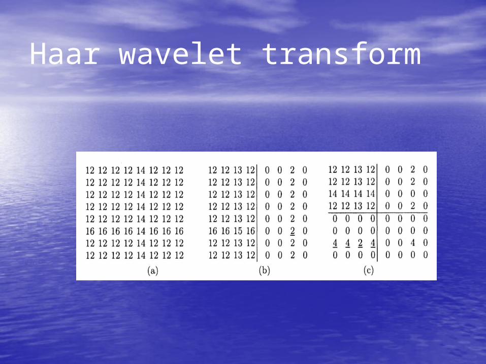
Haar wavelet transform
• Haar wavelet transform:
Average : resolutionDifference : detail
Example for one dimension

Haar wavelet transform
• Example: data=(5 7 6 5 3 4 6 9)
-average:(5+7)/2, (6+5)/2, (3+4)/2, (6+9)/2
-detail coefficients:
(5-7)/2, (6-5)/2, (3-4)/2, (6-9)/2
• n’= (6 5.5 3.5 7.5 | -1 0.5 -0.5 -1.5)
• n’’= (23/4 22/4 | 0.25 -2 -1 0.5 -0.5 -1.5)
• n’’’= (45/8 | 1/8 0.25 -2 -1 0.5 -0.5 -1.5)
Haar wavelet transform

Subband Transform
• The standard image wavelet transform• The Pyramid image wavelet transform

Subband Transform
HL
LH HH
LL

Wavelet Transform and Filter Banks
h0(n) is scaling function, low pass filter (LPF)
h1(n) is wavelet function, high pass filter (HPF)
is subsampling (decimation)

2-D Wavelet transform
H0
H1
2
x
a0
a12
H0
H1
2a00
a012
H0
H1
2a10
a112
Horizontal filtering Vertical filtering

Subband Transform

2-D wavelet transform
HH1
LH2
HL1
HL2
LH1
HH2
HH3
HH4
LL3

Software Research
Wavelet Coding

Wavelet Transform
Put a pixel in each quadrant- No size change
1 2
3 4
Software Research
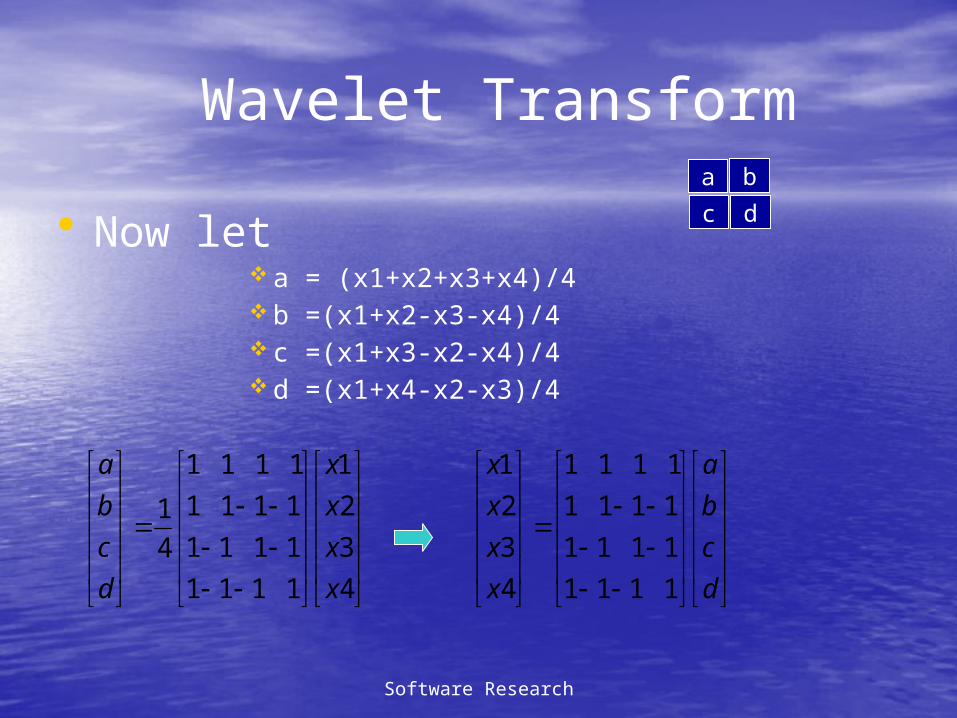
• Now let a = (x1+x2+x3+x4)/4 b =(x1+x2-x3-x4)/4 c =(x1+x3-x2-x4)/4 d =(x1+x4-x2-x3)/4
Wavelet Transforma b
c d
d
c
b
a
x
x
x
x
x
x
x
x
d
c
b
a
1111
1111
1111
1111
4
3
2
1
4
3
2
1
1111
1111
1111
1111
4
1

Wavelet Transform

Wavelet Transform

Wavelet Transform

2-D Example

Wavelet Transform

JPEG 2000 Image Compression Standard
JPEG 2000
• JPEG 2000 is a new still image compression standard• ”One-for-all” image codec:
* Different image types: binary, grey-scale, color,
multi-component
* Different applications: natural images, scientific,
medical remote sensing text, rendered graphics
* Different imaging models: client/server, consumer
electronics, image library archival, limited buffer
and resources.
History
• Call for Contributions in 1996• The 1st Committee Draft (CD) Dec. 1999• Final Committee Draft (FCD) in March 2000• Accepted as Draft International Standard in Aug. 2000• Published as ISO Standard in Jan. 2002
Key components
• Transform– Wavelet – Wavelet packet– Wavelet in tiles
• Quantization– Scalar
• Entropy coding– (EBCOT) code once, truncate anywhere – Rate-distortion optimization– Context modeling– Optimized coding order

Key components
Visual Weighting Masking
Region of interest (ROI)Lossless color transformError resilienceThe codestream obtained after compression of an image with JPEG 2000 is scalable in nature, meaning that it can be decoded in a number of ways; for instance, by truncating the codestream at any point, one may obtain a representation of the image at a lower resolution, or signal-to-noise ratio

JPEG 2000: A Wavelet-Based New Standard
• Targets and features– Excellent low bit rate performance without sacrifice performance
at higher bit rate– Progressive decoding to allow from lossy to lossless
• For details– David Taubman: “High Performance Scalable Image Compression
with EBCOT”, IEEE Trans. On Image Proc, vol.9(7), 7/2000.– JPEG2000 Tutorial by Skrodras @ IEEE Sig. Proc Magazine 9/2001 – Taubman’s book on JPEG 2000 (on library reserve)– Links and tutorials @ http://www.jpeg.org/JPEG2000.htm

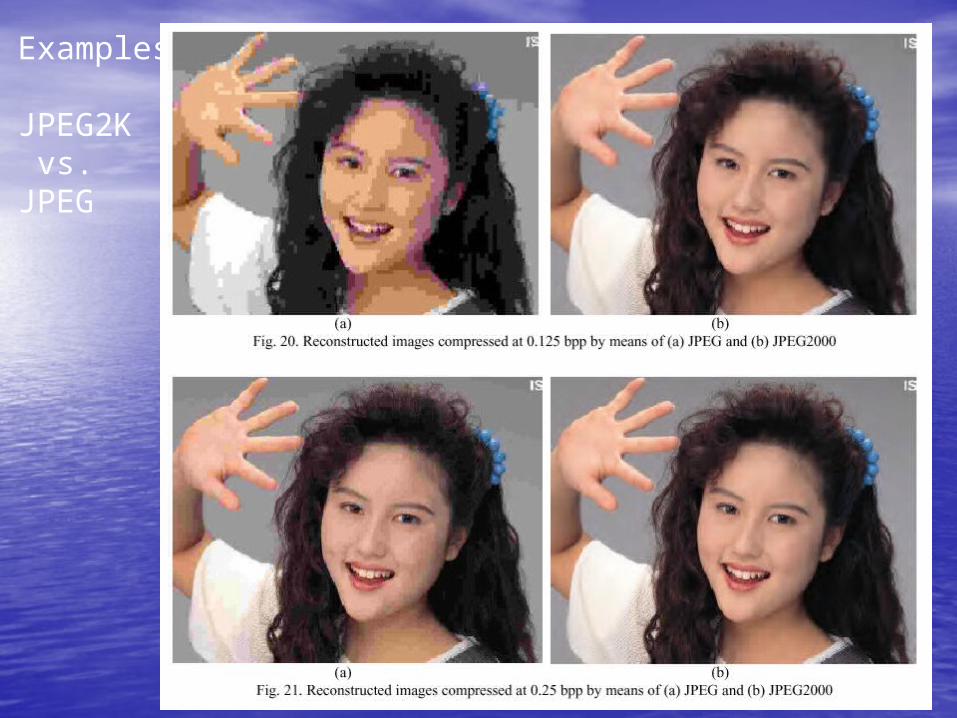
Superior compression performance: at high bit rates, where artifacts become nearly imperceptible, JPEG 2000 has a small machine-measured fidelity advantage over JPEG.
At lower bit rates (e.g., less than 0.25 bits/pixel for grayscale images), JPEG 2000 has a much more significant advantage over certain modes of JPEG: artifacts are less visible and there is almost no blocking
Multiple resolution representation: JPEG 2000 decomposes the image into a multiple resolution representation in the course of its compression process.
This representation can be put to use for other image presentation purposes beyond compression as such.
Progressive transmission by pixel and resolution accuracy, commonly referred to as progressive decoding and signal-to-noise ratio (SNR) scalability: JPEG 2000 provides efficient code-stream organizations which are progressive by pixel accuracy and by image resolution (or by image size).
This way, after a smaller part of the whole file has been received, the viewer can see a lower quality version of the final picture.
The quality then improves progressively through downloading more data bits from the source.


2-D wavelet transform
Original128, 129, 125, 64, 65, …
Transform Coeff.4123, -12.4, -96.7, 4.5, …

Quantization of wavelet coefficients
Transform Coeff.4123, -12.4, -96.7, 4.5, …
Quantized Coeff.(Q=64)64, 0, -1, 0, …

Entropy coding
0 1 1 0 1 1 0 1 0 1 . . .
Coded Bitstream
Quantized Coeff.(Q=64)64, 0, -1, 0, …

EBCOT
• Key features of EBCOT: Embedded Block Coding with Optimized Truncation– Low memory requirement in coding and
decoding– Easy rate control– High compression performance– Region of interest (ROI) access– Error resilience– Modest complexity

Block structure in EBCOT
Encode each block separately & record the bitstream of each block.Block size is 64x64.
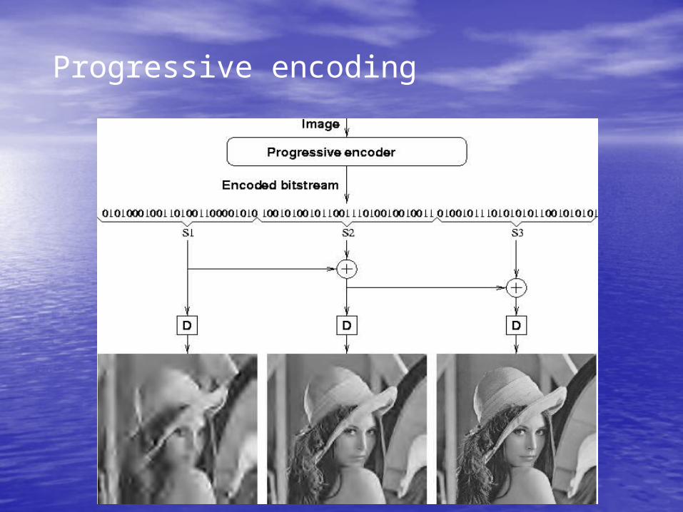
Progressive encoding
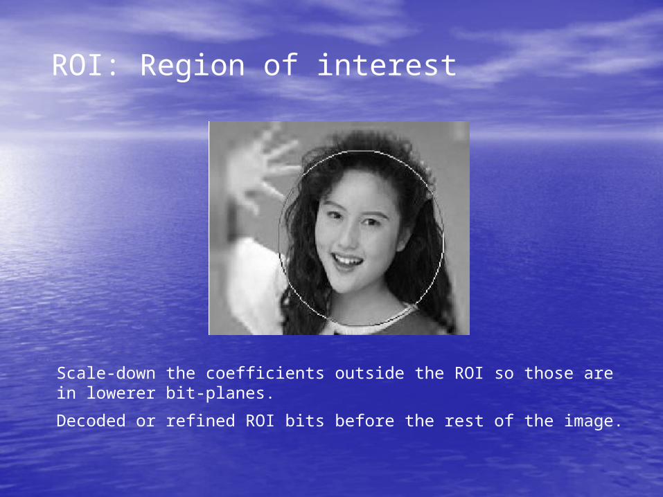
ROI: Region of interest
Scale-down the coefficients outside the ROI so those are in lowerer bit-planes.
Decoded or refined ROI bits before the rest of the image.

ROI: Region of interest
• Sequence based code– ROI coefficients are coded as independent
sequences– Allows random access to ROI without fully
decoding– Can specify exact quality/bitrate for ROI and the
BG• Scaling based mode:
– Scale ROI mask coefficients up (decoder scales down)
– During encoding the ROI mask coefficients are found significant at early stages of the coding
– ROI always coded with better quality than BG– Can't specify rate for BG and ROI

Tiling
• Image Component Tile Subband Code-Block Bit-Planes
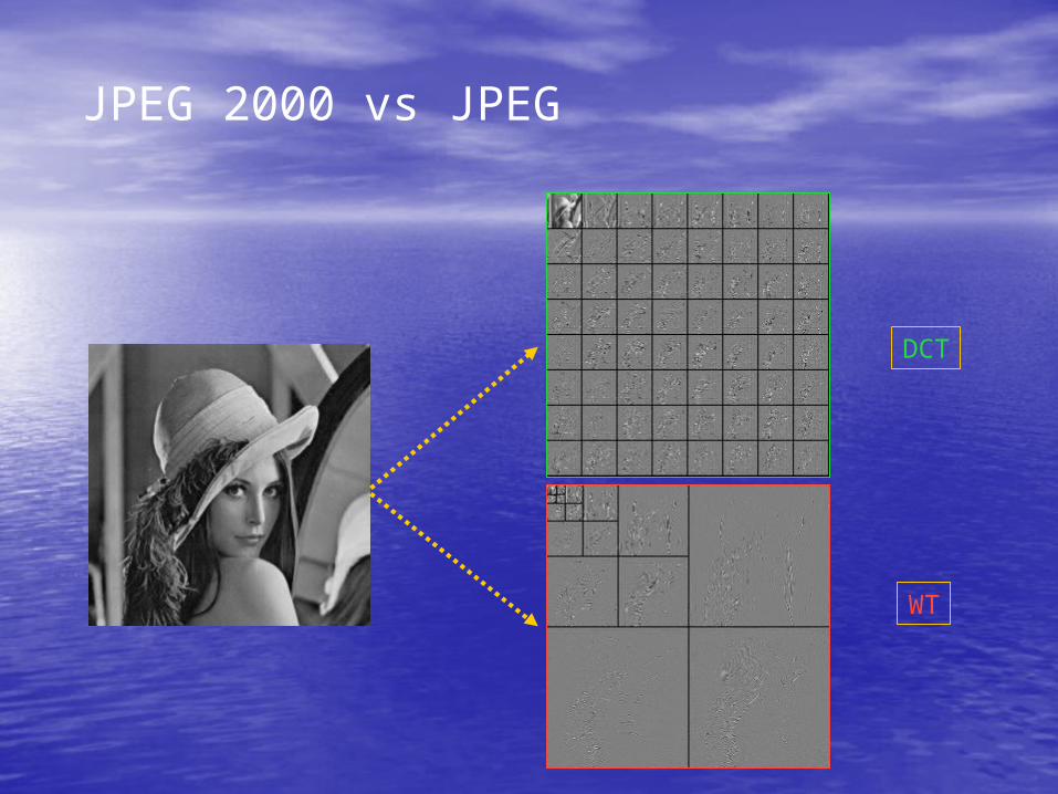
JPEG 2000 vs JPEG
DCT
WT

JPEG 2000 vs JPEG: Quantization
JPEG
JPEG 2000
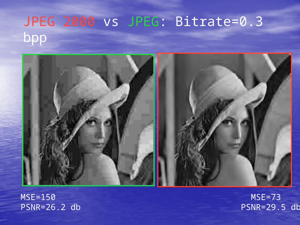
JPEG 2000 vs JPEG: Bitrate=0.3 bpp
MSE=150 MSE=73PSNR=26.2 db PSNR=29.5 db

JPEG 2000 vs JPEG: Bitrate=0.2 bpp
MSE=320 MSE=113PSNR=23.1 db PSNR=27.6 db
Lec14 – Wavelet Coding [66]
Examples
JPEG2K vs. JPEG

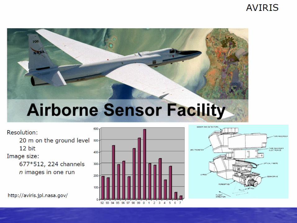

- 17 Mbps data rate through 1994, 20.4 Mbps from 1995 to 2004, 16 bit from 2005 onward- 10 bit data encoding through 1994, 12 bit from 1995- Silicon (Si) detectors for the visible range, indium gallium arsenide (InGaAr) for the NIR, and indium-antimonide (InSb) detectors for the SWIR- "Whisk broom" scanning- 12 Hz scanning rate- Liquid Nitrogen (LN2) cooled detectors- 10 nm nominal channel bandwidth, calibrated to within 1 nm- 34 degrees total field of view (full 677 samples)- 1 milliradian Instantaneous Field Of View (IFOV, one sample), calibrated to within 0.1 mrad- 76GB hard disk recording medium


The End