Macroprudential Policy in a DSGE Model: anchoring the countercyclical capital buffer

Leonardo Nogueira Ferreira and Márcio Issao Nakane

November, 2015

407

ISSN 1518-3548 CGC 00.038.166/0001-05

Working Paper Series Brasília n. 407 November 2015 p. 1-24

Working Paper Series

Edited by Research Department (Depep) – E-mail: workingpaper@bcb.gov.br

Editor: Francisco Marcos Rodrigues Figueiredo – E-mail: francisco-marcos.figueiredo@bcb.gov.br

Editorial Assistant: Jane Sofia Moita – E-mail: jane.sofia@bcb.gov.br

Head of Research Department: Eduardo José Araújo Lima – E-mail: eduardo.lima@bcb.gov.br

The Banco Central do Brasil Working Papers are all evaluated in double blind referee process.

Reproduction is permitted only if source is stated as follows: Working Paper n. 407.

Authorized by Altamir Lopes, Deputy Governor for Economic Policy.

General Control of Publications

Banco Central do Brasil

Comun/Dipiv/Coivi

SBS – Quadra 3 – Bloco B – Edifício-Sede – 14º andar

Caixa Postal 8.670

70074-900 Brasília – DF – Brazil

Phones: +55 (61) 3414-3710 and 3414-3565

Fax: +55 (61) 3414-1898

E-mail: editor@bcb.gov.br

The views expressed in this work are those of the authors and do not necessarily reflect those of the Banco Central or

its members.

Although these Working Papers often represent preliminary work, citation of source is required when used or reproduced.

As opiniões expressas neste trabalho são exclusivamente do(s) autor(es) e não refletem, necessariamente, a visão do Banco

Central do Brasil.

Ainda que este artigo represente trabalho preliminar, é requerida a citação da fonte, mesmo quando reproduzido parcialmente.

Citizen Service Division

Banco Central do Brasil

Deati/Diate

SBS – Quadra 3 – Bloco B – Edifício-Sede – 2º subsolo

70074-900 Brasília – DF – Brazil

Toll Free: 0800 9792345

Fax: +55 (61) 3414-2553

Internet: <http//www.bcb.gov.br/?CONTACTUS>

Macroprudential Policy in a DSGE Model: anchoring thecountercyclical capital buffer

Leonardo Nogueira Ferreira*

Marcio Issao Nakane**

Abstract

The Working Papers should not be reported as representing the views of the Banco Centraldo Brasil. The views expressed in the papers are those of the author(s) and not necessarilyreflect those of the Banco Central do Brasil.

The 2007-8 world financial crisis highlighted the deficiency of the regulatory frame-work in place at the time. Thenceforth many papers have been assessing the intro-duction of macroprudential policy in a DSGE model. However, they do not focuson the choice of the variable to which the macroprudential instrument must respond- the anchor variable. In order to fulfil this gap, we input different macroprudentialrules into the DSGE with a banking sector proposed by Gerali et al. (2010), and es-timate its key parameters using Bayesian techniques applied to Brazilian data. Wethen rank the results using the unconditional expectation of lifetime utility as of timezero as the measure of welfare: the larger the welfare, the better the anchor variable.We find that credit growth is the variable that performs best.

Keywords:Macroprudential Policy, Basel III, Capital Buffer, Anchor VariableJEL Classification: E3, E5

*Department of Financial System Regulation, Banco Central do Brasil, e-mail:leonardo.ferreira@bcb.gov.br

**Department of Economics, University of Sao Paulo, Brazil, e-mail: minakane@usp.br

3

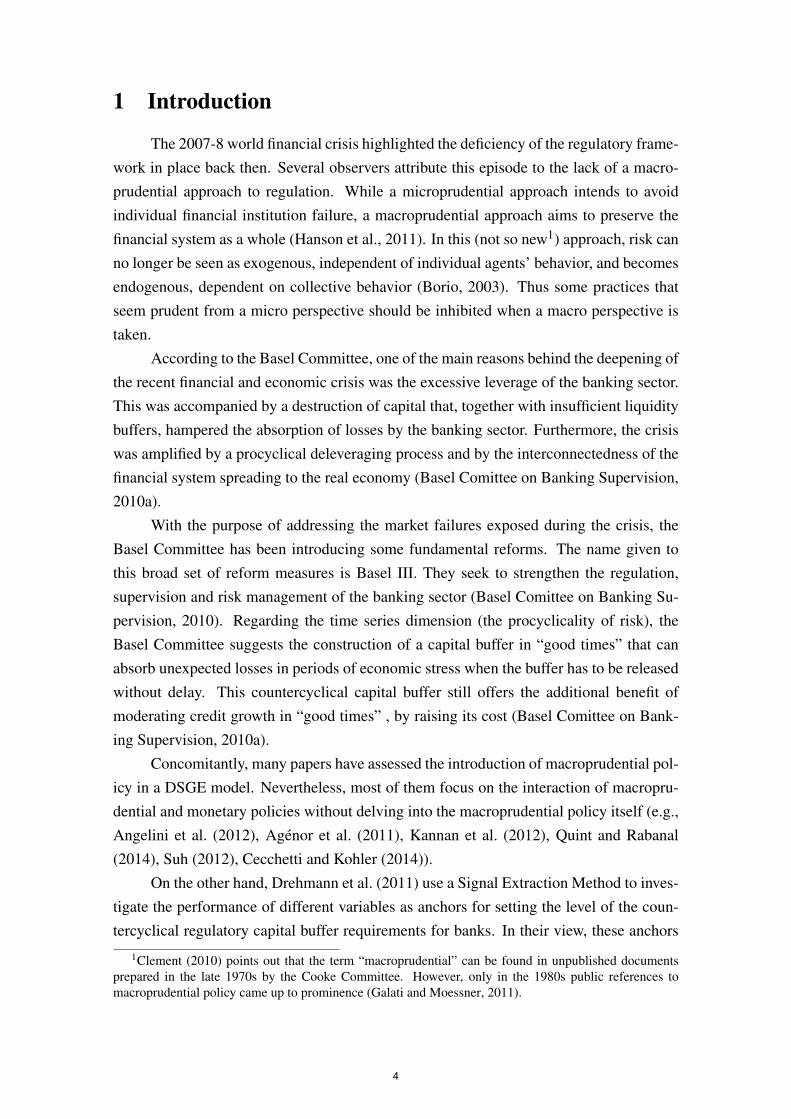
1 Introduction

The 2007-8 world financial crisis highlighted the deficiency of the regulatory frame-work in place back then. Several observers attribute this episode to the lack of a macro-prudential approach to regulation. While a microprudential approach intends to avoidindividual financial institution failure, a macroprudential approach aims to preserve thefinancial system as a whole (Hanson et al., 2011). In this (not so new1) approach, risk canno longer be seen as exogenous, independent of individual agents’ behavior, and becomesendogenous, dependent on collective behavior (Borio, 2003). Thus some practices thatseem prudent from a micro perspective should be inhibited when a macro perspective istaken.

According to the Basel Committee, one of the main reasons behind the deepening ofthe recent financial and economic crisis was the excessive leverage of the banking sector.This was accompanied by a destruction of capital that, together with insufficient liquiditybuffers, hampered the absorption of losses by the banking sector. Furthermore, the crisiswas amplified by a procyclical deleveraging process and by the interconnectedness of thefinancial system spreading to the real economy (Basel Comittee on Banking Supervision,2010a).

With the purpose of addressing the market failures exposed during the crisis, theBasel Committee has been introducing some fundamental reforms. The name given tothis broad set of reform measures is Basel III. They seek to strengthen the regulation,supervision and risk management of the banking sector (Basel Comittee on Banking Su-pervision, 2010). Regarding the time series dimension (the procyclicality of risk), theBasel Committee suggests the construction of a capital buffer in “good times” that canabsorb unexpected losses in periods of economic stress when the buffer has to be releasedwithout delay. This countercyclical capital buffer still offers the additional benefit ofmoderating credit growth in “good times” , by raising its cost (Basel Comittee on Bank-ing Supervision, 2010a).

Concomitantly, many papers have assessed the introduction of macroprudential pol-icy in a DSGE model. Nevertheless, most of them focus on the interaction of macropru-dential and monetary policies without delving into the macroprudential policy itself (e.g.,Angelini et al. (2012), Agenor et al. (2011), Kannan et al. (2012), Quint and Rabanal(2014), Suh (2012), Cecchetti and Kohler (2014)).

On the other hand, Drehmann et al. (2011) use a Signal Extraction Method to inves-tigate the performance of different variables as anchors for setting the level of the coun-tercyclical regulatory capital buffer requirements for banks. In their view, these anchors

1Clement (2010) points out that the term “macroprudential” can be found in unpublished documentsprepared in the late 1970s by the Cooke Committee. However, only in the 1980s public references tomacroprudential policy came up to prominence (Galati and Moessner, 2011).

4

are best used as leading indicators for boom periods, when the capital requirement shouldbe increased, and coincident indicators for credit crunches, when it should be releasedalmost immediately.

Drehmann et al. (2011) conclude that the best leading indicator is credit-to-GDPgap, whereas the best coincident indicator is banking spread. Still, the Basel Committeesuggests the use of credit-to-GDP gap as an anchor variable for both periods. However,Repullo and Saurina (2011) argue that the use of such variable may exacerbate procycli-cality inherent in the financial system and recommend the use of output growth.

To our knowledge, there are no papers that utilize a DSGE model to inquire intothe effects of different anchors in the countercyclical capital requirement rule (from nowon just macroprudential rule) on some important macroeconomic variables. The availablestudies simply take a given rule for granted, and then proceed to the step where theyevaluate its effects and relationship to monetary policy.

In order to fulfil this gap and to bring together the two literatures, we input differentmacroprudential rules into the DSGE proposed by Gerali et al. (2010), which has helpfulfeatures for our purpose. First, it incorporates an imperfectly competitive banking sectorand its interaction with the real economy. Second, it is estimated, which allow us torecover the parameters driving the banking dynamics (Angelini et al., 2012).

With the aim of comparing alternative macroprudential rules, we analyse the welfare-maximizing optimal policy using the second order approximation of the equilibrium as inSchmitt-Grohe and Uribe (2007). We measure welfare as the unconditional expectationof lifetime utility as of time zero, and then we rank the results: the larger the welfare, thebetter the anchor variable.

Credit growth is the variable that performs best. This variable is the most effectivein reducing the transmission of the higher costs banks face after a capital destruction tothe interest rate and hence in slowing down the weakening in demand for credit.

Since DSGE models can be used to analyse and understand the mechanisms throughwhich exogenous shocks (e.g., destruction of bank capital) are transmitted to the realeconomy, how macro variables react to aggregate shocks and the transmission channelsof different economic policies, we believe that it is important to complement the analysismade by Drehmann et al. (2011) addressing the choice of the anchor variable in a DSGE(Basel Comittee on Banking Supervision, 2012).

The model is estimated for the Brazilian economy. Brazil is an important emergingmarket and it is an interesting case study for the issues raised in this paper. Brazil has beenan early adopter of macroprudential tools and has been widely recognized by its promptreaction to the 2007-8 financial turmoil (International Monetary Fund, 2013). Moreover,there are few papers that measure the impact of macroprudential policy on the Brazilianeconomy using DSGE models: Kanczuk (2013), Carvalho et al. (2013) and Carvalho and

5

Castro (2015).The rest of the paper is organized as follows. Section 2 describes the model. In

Section 3 we describe the data and we present the results of the estimation. Section 4presents the application and the welfare analysis. Section 5 concludes.

2 Model

We take the DSGE model developed in Gerali et al. (2010) as the reference for ouranalysis. Angelini et al. (2012) have already introduced a macroprudential rule in thismodel, but they do not focus on the choice of the anchor variable.

Gerali et al. (2010) add monopolistically competitive banks to a model with creditfrictions and borrowing constraints as in Iacoviello (2005) and a set of real and nominalfrictions as in Christiano et al. (2005) and Smets and Wouters (2003). It fits well to Brazilbecause there is evidence that Brazilian banks are positioned somewhere between perfectcompetition and cartel arrangement showing some market power (Nakane, 2002).

The economy is populated by patient and impatient households, and by entrepreneurs.Patient households deposit their savings in banks. Impatient households and entrepreneursborrow, subject to a binding collateral constraint. All households consume, work and ac-cumulate housing, while entrepreneurs produce consumer and investment goods usingcapital and labor as inputs.

Banks set interest rates on deposits and on loans in order to maximize profits. Theirassets include loans to firms and to households, and their liabilities are deposits and capi-tal. Banks also face a balance-sheet constraint: there is a target for capital-to-assets ratiothey have to observe. This target (set at a fixed level in Gerali et al. (2010)) is preciselyour macroprudential instrument.

We reproduce here only the key equations for the complete understanding of theway macroprudential policy operates. For a detailed description of the model see Geraliet al. (2010).

2.1 Agents

Households consume, work and accumulate housing. The heterogeneity in agents’discount factors generates positive financial flows in equilibrium. Patient households havelarger discount factors and will be net savers in equilibrium whereas impatient householdswill be net borrowers in equilibrium. Households provide differentiated labor types, soldby unions to perfectly competitive labor packers who assemble them in a CES aggregatorand sell the homogeneous labor to entrepreneurs. Nominal wages are set by unions towhich workers belong.

6

The representative patient household i maximizes:

E0

∞

∑t=0

βtP

[(1−aP)εz

t log(cPt (i)−aPcP

t−1)+ εht loghP

t (i)−lPt (i)

1+φ

1+φ

](1)

which depends on individual current consumption cPt (i), lagged aggregate consumption

cPt , housing hP

t (i) and hours worked lPt (i). The parameters aP and φ measure, respectively,

the degree of external habit formation and the inverse Frisch elasticity of labor supply. Thebudget constraint (in real terms) must be met:

cPt (i)+qh

t ∆hPt (i)+dP

t (i)≤ wPt lP

t (i)+(1+ rdt−1)

dPt−1

πt+ tP

t (i) (2)

where qht is the real house price, dP

t are the deposits, rdt is the interest rate on last period

deposits, wPt is the real wage, πt is the gross inflation and tP

t are the lump-sum transfersthat include a labor union membership net fee and dividends from firms and banks (ofwhich patient households are the only owners).

The optimal choice between consumption and savings is given by the followingequation:

(1−aP)εzt

cPt −aPcP

t−1= βPEt

[(1−ap)εz

t+1

cPt+1−aPcP

t

1+ rdt

πt+1

](3)

which depends on the return on deposits.The representative impatient household i maximizes:

E0

∞

∑t=0

βtI

[(1−aI)εz

t log(cIt (i)−aIcI

t−1)+ εht loghI

t (i)−lIt (i)

1+φ

1+φ

](4)

with no change beyond the superscript that indexes the type of agent. The followingbudget constraint must be met:

cIt (i)+qh

t ∆hIt (i)+(1+ rbH

t−1)bI

t−1(i)πt

≤ wPt lI

t (i)+bIt (i)+ tP

t (i) (5)

in which resources spent on consumption, housing, and gross repayment of borrowingbI

t−1 (with a net interest rate of rbHt−1) have to be funded with labor income (wI

t is the wageof impatient households) and new loans bI

t (tIt only includes net union fees).

Impatient households face an additional borrowing constraint:

(1+ rbHt )bI

t (i)≤ mIt Et [qh

t+1hIt (i)πt+1] (6)

where mIt is the loan-to-value ratio. This borrowing constraint implies that the expected

7

value of their housing stock must ensure payment of debt and interests. Actually, housingcan represent the consumption of non-durable goods. That is why collateral constraintsappear to be a good approximation of credit markets in Brazil. Almost half of the loansto households in Brazil are collateralized (Banco Central do Brasil, 2013a) 2.

The optimal choice for the impatient household is given by the following equation:

(1−aI)εzt

cIt −aIcI

t−1= βIEt

[(1−aI)εz

t+1

cIt+1−aPcI

t

1+ rbHt

πt+1

]+λ

Ht (1+ rbH

t ) (7)

Such choice depends on the expected real cost of new loans and on the Lagrange multi-plier associated with the collateral constraint (λ H

t ). λ Ht is the increase in lifetime utility

resulting from borrowing extra loans and reducing consumption next period. Combiningthe patient’s steady-state Euler equation with the impatient’s steady-state Euler equationreturns:

λH =

βPM −βI

πcI (8)

where M is the markup over gross interest rate on deposits.As the economy features imperfectly competitive banking sector and financial fric-

tions, the usual assumption βP > βI is no longer sufficient to guarantee that impatienthouseholds are constrained around the steady state. The larger M, the larger the dif-ference in agents’ discount factors must be for the constraint to be binding around thesteady state . The same reasoning applies to the Lagrange multiplier associated with theentrepreneur’s borrowing constraint.

The expected utility of entrepreneurs depends only on consumption cEt :

E0

∞

∑t=0

βtE log

(cE

t (i)−aEcEt−1)

(9)

This expected utility is maximized subject to the budget constraint:

cEt (i)+wP

t lE,Pt (i)+wI

t lE,It (i)+

(1+ rbE

t−1

) bEt−1(i)πt

+qkt kE

t (i)+ψ(ut(i))kEt−1(i) =

yEt (i)xt

+bEt (i)+qk

t (1−δ )kEt−1(i) (10)

in which δ is the depreciation rate of capital kE , qkt is the price of capital in terms of

consumption, ψ(ut(i))kEt−1(i) is the real cost of setting a level ut of utilization rate , 1

x isthe relative competitive price of the wholesale good yE produced from technology, capital

2Vehicle financing, Leasing and Real estate financing. Despite the fact that part of the latter are directedloans that affect the transmission channels, we decided to keep the model simple and focus only on non-regulated loans.

8

and a combination of labor supplied by patient and impatient households, and rBEt is the

interest rate on loans to entrepreneurs bEt .

Entrepreneurs are also subject to a borrowing constraint:

(1+ rbEt )bE

t (i)≤ mEt Et [qk

t+1πt+1(1−δ )kEt (i)] (11)

i.e., the expected value of the capital stock must guarantee payment of debt and interests.The optimal choice for the entrepreneur is given by the following Euler equation:

(1−aE)

cEt −aEcE

t−1= βPEt

[(1−aE)

cEt+1−aEcE

t

1+ rbEt

πt+1

]+λ

Et (1+ rbE

t ) (12)

Such choice depends on the expected real cost of new loans and on the Lagrange multi-plier associated with the collateral constraint (λ E

t ).

2.2 Banks

Each bank in the model is composed of two “retail” branches and one “wholesale”unit. One retail unit provides differentiated loans to entrepreneurs and households andthe other unit raises differentiated deposits. The wholesale unit is responsible for man-aging the bank’s capital position. Banks accumulate capital out of earnings of the threebranches, as follows:

πtKbt = (1−δ

b)Kbt−1 + jb

t−1 (13)

in which Kbt is the bank capital, πt is the gross inflation, jb

t are overall real profits and δ b

is the depreciation rate. Bank capital establishes a link, crucial to the model, between thecredit supply and the economic cycle. In “good” times, retained earnings increase bankcapital stock allowing the soaring of loans, while in “bad” times, when profits are smaller,bank capital shrinks leading to a contraction of loan supply further fuelling the crisis.

The maximization problem for the wholesale unit is to choose loans and deposits.The resulting wholesale interest rate on loans to credit-constrained households and en-trepreneurs is as follows:

Rbt = Rd

t −κ

(Kb

tBt− vt

)(Kb

tBt

)2

(14)

where Rbt is the net wholesale loan rate, Rd

t is the net wholesale deposit rate, vt the targetfor their capital-to-assets ratio, κ parameterizes the quadratic cost paid by the banks whenthey deviate from the target vt and Bt is the sum of risk-weighted loans to entrepreneurs

9

and to households. According to Angelini et al. (2012), Bt has the following specification:

Bt = wEt BE

t +wHt BH

t (15)

where wt is the cyclical risk which is modelled as:

wit = (1−ρi)wi +(1−ρi)χi(yt− yt−4)+ρiwi

t−1 i = I,E (16)

where y is output and ρi is the inertia in risk and χi is the response to annual output growth.The steady state of wi

t is 1.When loans increase, the capital-to-assets ratio falls below vt , leading banks to raise

Rbt , which contributes to reduction of the demand for credit.

It is assumed that banks have access to unlimited finance at policy rate rt . Thus, byarbitrage, Rd

t = rt and then we have:

Swt ≡ Rb

t − rt =−κ

(Kb

tBt− vt

)(Kb

tBt

)2

(17)

where Swt is the spread at the wholesale level. The left-hand side of the equation repre-

sents the marginal benefit of an increase in loans while the right-hand side represents themarginal cost of its increase, because the bank would be farther from the target vt . Thus,banks choose to operate at the point that equalizes the benefits and the costs of reducingthe capital-to-assets ratio.

The retail loan branch applies a markup over the wholesale rate. The retail interestrate on loans to credit-constrained households and entrepreneurs is as follows:

rbst =

εbst

εbst −1

Rbt +Ad jbs

t =⇒ rbst =

εbst

εbst −1

[rt−κ

(Kb

tBt− vt

)(Kb

tBt

)2]+Ad jbs

t (18)

where εbst > 1 is the elasticity of loan demand and s indexes the agent, and Ad jbs

t capturesthe cost of adjusting loan rates.

It is assumed, as in Carvalho et al. (2013), that there is no markdown over the policyrate:

rdt = rt (19)

Loan demand elasticities are decisive in determining the spreads between the policyrate and the retail ones. To sum up, the deposit branch raises deposits, the wholesalebranch determines its lending rate, which depends on the capital-to-assets ratio, and uponwhich the loan branch applies a markup to determine the interest rate on loans to impatienthouseholds and entrepreneurs.

The bank’s trade-off can also be seen in the equation that shows overall bank profits

10

(in real terms). It is easy to see that the greater the distance between Kbt

Btand vt , the lower

the bank profits. However, the larger bHt and bE

t , the higher the profits:

jbt = rbH

t bHt + rbE

t bEt − rd

t dt−κ

(Kb

tBt− vt

)2

Kbt −Ad jB

t (20)

where rbHt is the interest rate on loans to households, rbE

t is the interest rate on loans toentrepreneurs, rd

t is the interest rate on deposits and Ad jBt captures the costs of adjusting

interest rates.As the business cycle affects bank profits and, therefore, capital (accumulated out

of retained earnings), there is room for active policies aiming to mitigate its effects on thereal economy.

2.3 Macroprudential and Monetary Policies

The central bank is assumed to follow a standard Taylor rule:

rt = (1−ρR)r+(1−ρR)[χπ(πt− π)+χy(yt− yt−1)]+ρRrt−1 + εRt (21)

where r is the steady-state policy rate, ρR is the inertia in the adjustment of the policyrate, χπ measures the response to deviations of inflation π to the target(π), χy measuresthe response to output growth (yt) and εR

t is the monetary policy shock.Our macroprudential instrument is the countercyclical capital buffer. We follow

Angelini et al. (2012):

vt = (1−ρv)v+(1−ρv)χvXt +ρvvt (22)

where v is the steady-state level of vt , ρv is the inertia in the adjustment of the counter-cyclical capital buffer and Xt is a macroeconomic variable with sensibility χv. Xt is whatwe call anchor variable. Anchor variables can be seen as proxies for the cyclicality thatthe instrument is designed to mitigate.

Angelini et al. (2012) point out that the capital requirement is a good macropruden-tial instrument for two reasons. Primarily, based on recent experience, systemic crisesaffect bank capital and credit supply directly or indirectly. Additionally, bank capital is atthe hub of the current debate on regulatory reform.

Equations (18) and (19) show that monetary and macroprudential policies have po-tentially different roles. Policy rate affects the deposit rate and the loan rate; macropru-dential policy only affects the loan rate giving greater freedom to the policymaker. If thereis a need to affect differently savers and borrowers, the authority in question can changeonly vt .

11

3 Estimation

We apply standard Bayesian Methods to estimate model parameters without macro-prudential policy 3. Bayesian estimation is a bridge between calibration and maximumlikelihood: priors can be seen as weights on the likelihood function in order to give moreimportance to certain areas of the parameter subspace (Griffoli, 2007).

There are many advantages of using Bayesian methods to estimate a model. First,Bayesian estimation fits the DSGE model. Second, Bayesian techniques prevent the pos-terior distribution from peaking at strange points where the likelihood peaks. Third, theinclusion of priors helps identifying parameters (Griffoli, 2007).

Since there is not much literature regarding the parameters driving the banking dy-namics in Brazil, we decided to focus our estimation on these parameters, while we cali-brate the others. In this section, we present the data, the calibrated parameters, the priorand the posterior distributions.

3.1 Data

The model is estimated for the Brazilian economy. We use 9 observables: real con-sumption, real investment, inflation, deposits, loans to households and to firms, interestrates on loans to households and firms, and the overnight rate. For a detailed descriptionof the data, see the Appendix. The sample period is 2000q3-2012q4. Data with a trend aremade stationary using one-sided HP filter4, while inflation rate is demeaned and interestrates are demeaned using the mean overnight growth rate (Pfeifer, 2014). Figure 1 reportsthe transformed data.

Figure 1: Observed Variables Used in Estimation

3We only add macroprudential policy to the model after the estimation is complete. In the sample period,there was no countercyclical capital buffer in Brazil. Thus it is possible to properly recover some unknownparameters from the banking sector.

4Smoothing parameter equal to 1,600.

12

3.2 Calibrated Parameters

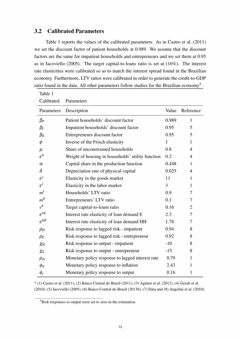
Table 1 reports the values of the calibrated parameters. As in Castro et al. (2011)we set the discount factor of patient households at 0.989. We assume that the discountfactors are the same for impatient households and entrepreneurs and we set them at 0.95as in Iacoviello (2005). The target capital-to-loans ratio is set at (16%). The interestrate elasticities were calibrated so as to match the interest spread found in the Brazilianeconomy. Furthermore, LTV ratios were calibrated in order to generate the credit-to-GDPratio found in the data. All other parameters follow studies for the Brazilian economy5.

Table 1Calibrated Parameters

Parameters Description Value Reference

βP Patient households’ discount factor 0.989 1βI Impatient households’ discount factor 0.95 5βE Entrepreneurs discount factor 0.95 5φ Inverse of the Frisch elasticity 1 1µ Share of unconstrained households 0.8 4εh Weight of housing in households’ utility function 0.2 4α Capital share in the production function 0.448 1δ Depreciation rate of physical capital 0.025 4εy Elasticity in the goods market 11 1ε l Elasticity in the labor market 3 1mI Households’ LTV ratio 0.9 7mE Entrepreneurs’ LTV ratio 0.1 7vb Target capital-to-loans ratio 0.16 2εbE Interest rate elasticity of loan demand E 2.3 7εbH Interest rate elasticity of loan demand HH 1.78 7ρH Risk response to lagged risk - impatient 0.94 8ρE Risk response to lagged risk - entrepreneur 0.92 8χH Risk response to output - impatient -10 8χE Risk response to output - entrepreneur -15 8ρib Monetary policy response to lagged interest rate 0.79 1φπ Monetary policy response to inflation 2.43 1φy Monetary policy response to output 0.16 1

* (1) Castro et al. (2011), (2) Banco Central do Brasil (2011), (3) Agenor et al. (2012), (4) Gerali et al.(2010), (5) Iacoviello (2005), (6) Banco Central do Brasil (2013b), (7) Data and (8) Angelini et al. (2010).

5Risk responses to output were set to zero in the estimation.

13

3.3 Prior and Posterior DistributionsTable 2Estimated Parameters

Prior PosteriorDist. Mean Std. Dev. Mean Median Std. Dev.

Structural Parametersκp Adj. cost for p Gamma 50 20 14.33 13.16 4.85κw Adj. cost for w Gamma 50 20 41.67 39.21 14.93ιp Degree of indexation of p Gamma 0.5 0.15 0.32 0.30 0.15ιw Degree of indexation of w Gamma 0.5 0.15 0.47 0.46 0.10κbe Firms’ rate adj. cost Gamma 3 2.5 0.30 0.28 0.11κbh HH’s rate adj. cost Gamma 6 2.5 0.17 0.16 0.05κkb Leverage dev. cost Gamma 20 5 23.15 22.96 2.63ai Habit coefficient Beta 0.5 0.1 0.68 0.69 0.08κi Investment adj. cost Gamma 2.5 1 3.40 3.31 0.74

Exogenous process: AR Coefficientsρz Consumpt. pref. Beta 0.8 0.1 0.44 0.44 0.08ρa Technology Beta 0.8 0.1 0.81 0.82 0.05ρmE Firms’ LTV Beta 0.8 0.1 0.90 0.91 0.04ρmH HH’s LTV Beta 0.8 0.1 0.93 0.94 0.03ρbH HH’s loans markup Beta 0.8 0.1 0.73 0.74 0.08ρbE Firms’ loans markup Beta 0.8 0.1 0.86 0.86 0.05ρqk Invest. efficiency Beta 0.8 0.1 0.56 0.55 0.08ρy p markup Beta 0.8 0.1 0.80 0.81 0.10ρKb Balance Sheet Beta 0.8 0.1 0.80 0.81 0.10

Exogenous process: Standard deviationsσz Consumpt. pref. Inv. G. 0.01 0.05 0.06 0.06 0.01σa Technology Inv. G. 0.01 0.05 0.01 0.01 0.01σmE Firms’ LTV Inv. G. 0.01 0.05 0.01 0.01 0.00σmH HH’s LTV Inv. G. 0.01 0.05 0.02 0.02 0.00σbH HH’s loans markup Inv. G. 0.01 0.05 0.51 0.50 0.06σbE Firms’ loans markup Inv. G. 0.01 0.05 0.27 0.27 0.03σqk Invest. Efficiency Inv. G. 0.01 0.05 0.05 0.05 0.01σR Monetary policy Inv. G. 0.01 0.05 0.01 0.01 0.00σy p markup Inv. G. 0.01 0.05 0.01 0.01 0.01σKb Balance Sheet Inv. G. 0.01 0.05 0.12 0.13 0.01

14

Table 2 presents the prior distributions. They follow mainly Gerali et al. (2010). Ta-ble 2 also reports the posterior mean and median, and the standard deviations of the esti-mated parameters. The posterior distribution was obtained using the Metropolis-Hastingsalgorithm. We ran 5 chains, each of 500,000 draws.

The habit coefficient and the investment adjustment cost values are close to thevalues found in Castro et al. (2011). The shocks are rather persistent. In the followingsection, parameter values are set at the posterior median.

4 Applications

This section discusses optimal macroprudential policy after an unexpected destruc-tion of 5% of bank capital. Such shock is introduced in the bank capital accumulationequation:

πtKbt = (1−δ

b)Kb

t−1

εkt

+ jbt−1 (23)

in which εkt is the financial shock6.

First, the anchor variables are ordered using a measure of welfare. Then the impulseresponse functions of the model that displays the best results will be presented. Thus, it ispossible to better understand the propagation mechanism of bank capital destruction, andthe best way to mitigate its effects.

4.1 Welfare

Welfare analyses have recently been increasingly used to measure the benefits ofmacroprudential policy (e.g., Rubio and Carrasco-Gallego (2014), Rubio and Carrasco-Gallego (2015), Laseen et al. (2015) ). The optimal combination of monetary and macro-prudential policies is here obtained by a second order approximation of the equilibrium.

The welfare measure is the unconditional expectation of average household utilitygiven initial values. Aggregated welfare is given by:

E0V = E0 {VP +VI +VE} (24)

in which VP is the expectation of patient households’ lifetime utility, VI is the expecta-tion of impatient households’ lifetime utility and VE is the expectation of entrepreneurs’lifetime utility.

As in Schmitt-Grohe and Uribe (2007) and Suh (2012), policy rules are easily im-plementable because they are functions of observable macroeconomic indicators. As

6For this exercise, we set v at 13%, the required level when the countercyclical capital buffer is on.

15

pointed out, the Taylor rule is standard:

rt = (1−ρR)r+(1−ρR)[χπ(πt− π)+χy(yt− yt−1)]+ρRrt−1 (25)

Macroprudential rule has a very similar format, being a function of the anchor variable:

vt = (1−ρv)v+(1−ρv)χvXt +ρvvt−1 (26)

Since there is more information in the literature about monetary policy parameters(χy and χπ ), they are restricted to a small range: χy between 0 and 3 and χπ between 1and 3. The macroprudential policy parameter, about which there is greater uncertainty, isrestricted to a broader range: (χv) between 0 and 10.

The range for χv is partinioned with grids of size 2 and the ranges for all the otherparameters are partitioned with grids of size 0.2. Macroprudential policies are assumedto have inertia (ρv = 0.9) (Suh, 2012). For each combination of parameters, the welfareE0V is calculated. The optimal policy is the one that presents the greatest welfare subjectto the ranges mentioned.

The anchor variables used in the exercise are some of the variables classified asmacroeconomic by the Basel Guide: GDP growth, credit growth, credit-to-GDP growth,risk-weighted credit growth, GDP gap, credit gap, credit-to-GDP gap and risk-weightedcredit gap. Then we have nine possible cases: “the monetary policy” (benchmark) andeight models with different anchor variables. The coefficients presented are those associ-ated with the optimal policy for each case.

Table 3 suggests that the introduction of macroprudential policy generates welfaregains. The variables are ranked according to the welfare: (1) is the variable that producesthe highest welfare and (5) the lowest. The “gap variables” have no benefit in terms ofwelfare compared to the case with only monetary policy7.

On the other hand, the more effective macroprudential policy in terms of welfareis the one which uses credit growth as an anchor variable. It is as if target and objectivecoincide: in order to avoid a drop in credit that would be detrimental to the economy, therelevant authority must be attentive to the behaviour of credit itself.

7We also run a model in which we set monetary policy parameters at the calibrated values (χy = 0.16and χπ = 2.43), allowing only χv to vary. The optimal choice for χv in this scenario is zero, but, as expected,the agents are worse off (they could have chosen these values, but they have not).

16

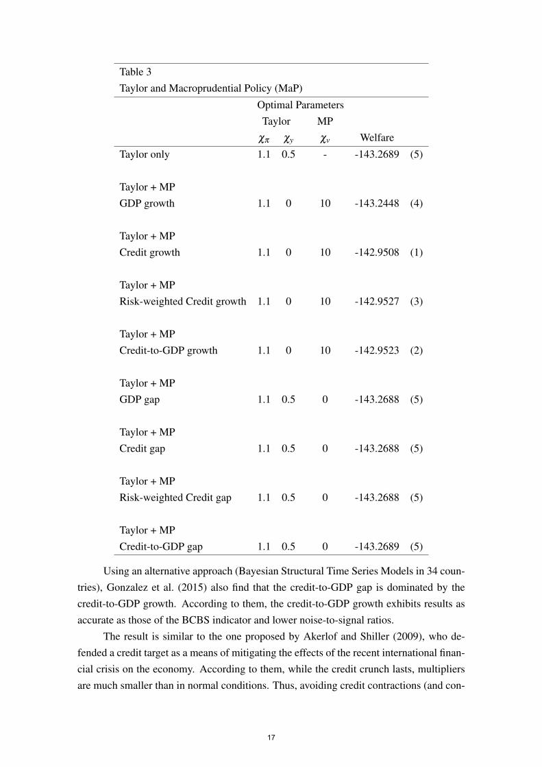
Table 3Taylor and Macroprudential Policy (MaP)

Optimal ParametersTaylor MP

χπ χy χv Welfare

Taylor only 1.1 0.5 - -143.2689 (5)

Taylor + MPGDP growth 1.1 0 10 -143.2448 (4)

Taylor + MPCredit growth 1.1 0 10 -142.9508 (1)

Taylor + MPRisk-weighted Credit growth 1.1 0 10 -142.9527 (3)

Taylor + MPCredit-to-GDP growth 1.1 0 10 -142.9523 (2)

Taylor + MPGDP gap 1.1 0.5 0 -143.2688 (5)

Taylor + MPCredit gap 1.1 0.5 0 -143.2688 (5)

Taylor + MPRisk-weighted Credit gap 1.1 0.5 0 -143.2688 (5)

Taylor + MPCredit-to-GDP gap 1.1 0.5 0 -143.2689 (5)

Using an alternative approach (Bayesian Structural Time Series Models in 34 coun-tries), Gonzalez et al. (2015) also find that the credit-to-GDP gap is dominated by thecredit-to-GDP growth. According to them, the credit-to-GDP growth exhibits results asaccurate as those of the BCBS indicator and lower noise-to-signal ratios.

The result is similar to the one proposed by Akerlof and Shiller (2009), who de-fended a credit target as a means of mitigating the effects of the recent international finan-cial crisis on the economy. According to them, while the credit crunch lasts, multipliersare much smaller than in normal conditions. Thus, avoiding credit contractions (and con-

17

sequently multipliers reduction), the need for too large fiscal and monetary stimulus isreduced.

However, the effects of the new policy differ among agents. If given a choice,patient consumers would prefer the regime in which only monetary policy operates, asit ensures greater welfare. On the other hand, entrepreneurs and impatient consumerswould choose the regime that combines monetary and macroprudential policies. Thus,the ordering of welfare is sensitive to changes in the weights.

Figure 2 displays the welfare when the anchor variable is credit growth. The axison the right side displays the range for χv and the axis on the left side displays the rangefor χy

8. The larger χv and the lower χy, the larger the welfare, implying that when theresponse of the countercyclical capital buffer to the anchor variable is strong, there is noneed for monetary policy to react.

Figure 2: Anchor: credit growth

The following subsection presents the impulse response functions of the model withcredit growth as an anchor variable. The parameters of monetary and macroprudentialpolicies were set at the associated optimal policy values (χy = 0, χπ = 1.1 and χv = 10)9.It will be compared to the model with only monetary policy that has the parameter valuesset at χy = 1.1 and χπ = 0.5.

8From 0 to 10 with grids of 2 results in 6 elements for the range of χv. The same reasoning applies forχy

9Taking into account the inertia parameter, this implies a response 4 times more reactive than the in-tended: according to (Basel Comittee on Banking Supervision, 2010b), when the gap is 10% or larger, thebuffer add-on is at its maximum (2.5%).

18

4.2 The Effects of a Bank Capital Loss

Figure 3 displays the impact of a bank capital loss on some important macroeco-nomic variables.

Figure 3: Anchor: credit growth versus Taylor only

After the shock, banks face higher costs linked to its capital position and pass it tothe interest rates on loans, weakening the demand for credit. The contraction of loansleads to a reduction in the level of investments and product. However, the interest ratecharged on loans to entrepreneurs increases less in the case with macroprudential policybecause the capital requirement also decreases, reducing costs related to the bank’s capitalposition. This, in turn, results in a lower decrease of loans when macroprudential policyoperates.

Thus, the performance of monetary and macroprudential policies reduces the impactthat the original destruction of bank capital has on the economy, mitigating the feedbackprocess. As in Gerali et al. (2010), the magnitude of the change in the trajectory ofvariables is greatly reduced. This occurs for two reasons. First, because the shock wascalibrated to generate a relatively small bank capital loss. Second, because the shock isunique and disregards other shocks potentially generated by it.

5 Conclusion

We have examined the process of choosing the best anchor variable in a DSGEmodel. Unlike studies that focus on the regulatory issue, our analysis was focused on thebehavior of macroeconomic variables and welfare. We believe that both aspects should

19

be complementary.In order to fulfil this gap, we input different macroprudential rules into the DSGE

proposed by Gerali et al. (2010). We estimate the model for the Brazilian economy, andthen we sort the results using a measure of welfare given by the unconditional expectationof lifetime utility as of time zero: the larger the welfare, the better the anchor variable.Credit growth is the variable that performs best.

It should be noted, however, that the difference between the variables in terms ofconsumption appears to be very low. So it is hard to say that the results are general. Morestudies are needed to make that assessment and even ask how relevant the welfare shouldbe when addressing financial regulatory issues.

20

References

Agenor, P., Alper, K., and da Silva, L. (2011). Capital regulation, monetary policy and

financial stability. Working Papers Series No 237, Central Bank of Brazil, Brazil.

Agenor, P.-R., Alper, K., and Pereira da Silva, L. (2012). Capital requirements and busi-ness cycles with credit market imperfections. Journal of Macroeconomics, 34(3):687–705.

Akerlof, G. A. and Shiller, R. J. (2009). The current financial crisis: What is to be done?In Animal Spirits: How Human Psychology Drives the Economy, and Why It Matters

for Global Capitalism. Princeton University Press, Princeton.

Angelini, P., Enria, A., Neri, S., Panetta, F., and Quagliariello, M. (2010). Pro-cyclicality

of capital regulation: is it a problem? How to fix it? Questioni di Economia e Finanza(Occasional Papers) No 74, Bank of Italy, Italy.

Angelini, P., Neri, S., and Panetta, F. (2012). Monetary and macroprudential policies.Working Paper Series No 1449, European Central Bank, Germany.

Banco Central do Brasil (2011). Relatorio de Estabilidade Financeira, volume 10. BancoCentral do brasil.

Banco Central do Brasil (2013a). Nota para a Imprensa: Polıtica Monetaria e Operacoes

de Credito do Sistema Financeiro. Banco Central do Brasil.

Banco Central do Brasil (2013b). Perguntas e Respostas sobre a Implantacao de Basileia

III no Brasil. Banco Central do Brasil.

Basel Comittee on Banking Supervision (2010a). Basel III: A global regulatory frame-

work for more resilient banks and banking systems. Bank for International Settlements,Basel.

Basel Comittee on Banking Supervision (2010b). Guidance for National Authorities Op-

erating the Countercyclical Capital Buffer. Bank for International Settlements, Basel.

Basel Comittee on Banking Supervision (2010). International regulatory framework for

banks (Basel III). Bank for International Settlements.

Basel Comittee on Banking Supervision (2012). Models and tools for macroprudential

analysis. BCBS Working paper No 21, Bank for International Settlements, Basel.

Borio, C. (2003). Towards a Macroprudential Framework for Financial Supervision and

Regulation? BIS Working Paper No 128, Bank for International Settlements, Basel.

21

Carvalho, F. A. and Castro, M. R. (2015). Foreign Capital Flows, Credit Growth and

Macroprudential Policy in a DSGE Model with Traditional and Matter-of-Fact Finan-

cial Frictions. Working Papers Series No 387, Central Bank of Brazil, Brazil.

Carvalho, F. A., Castro, M. R., and Costa, S. M. A. (2013). Traditional and Matter-

of-fact Financial Frictions in a DSGE Model for Brazil: the role of macroprudential

instruments and monetary policy. Working Papers Series No 336, Central Bank ofBrazil, Brazil.

Castro, M. R., Gouvea, S. N., Minella, A., dos Santos, R. C., and Souza-Sobrinho, N. F.(2011). SAMBA: Stochastic Analytical Model with a Bayesian Approach. WorkingPapers Series No 239, Central Bank of Brazil, Brazil.

Cecchetti, S. G. and Kohler, M. (2014). When capital adequacy and interest rate policyare substitutes (and when they are not). International Journal of Central Banking,10(3):205–232.

Christiano, L., Eichenbaum, M., and Evans, C. (2005). Nominal rigidities and the dy-namic effects of a shock to monetary policy. Journal of Political Economy, 113(1):1–45.

Drehmann, M., Borio, C., and Tsatsaronis, K. (2011). Anchoring countercyclical capital

buffers: the role of credit aggregates. BIS Working Paper No 355, Bank for Interna-tional Settlements, Basel.

Galati, G. and Moessner, R. (2011). Macroprudential policy–a literature review. BISWorking Paper No 337, Bank for International Settlements, Basel.

Gerali, A., Neri, S., Sessa, L., and Signoretti, F. M. (2010). Credit and banking in a DSGEmodel of the euro area. Journal of Money, Credit and Banking, 42(s1):107–141.

Gonzalez, R. B., Lima, J., and Marinho, L. (2015). Countercyclical Capital Buffers:

bayesian estimates and alternatives focusing on credit growth. Working Papers SeriesNo 384, Central Bank of Brazil, Brazil.

Griffoli, T. M. (2007). 2008. DYNARE User Guide: An Introduction to the solution &

estimation of DSGE models.

Hanson, S., Kashyap, A., and Stein, J. (2011). A macroprudential approach to financialregulation. The Journal of Economic Perspectives, 25(1):3–28.

Iacoviello, M. (2005). House prices, borrowing constraints, and monetary policy in thebusiness cycle. The American Economic Review, 95(3):739–764.

22

International Monetary Fund (2013). Brazil: Technical Note on Macroprudential Policy

Framework. IMF Country Report No. 13/148, Washington D.C.

Kanczuk, F. (2013). Um termometro para as macro-prudenciais. Revista Brasileira de

Economia, 67(4):464–489.

Kannan, P., Rabanal, P., and Scott, A. M. (2012). Monetary and macroprudential pol-icy rules in a model with house price booms. The B.E. Journal of Macroeconomics,12(1):16.

Laseen, S., Pescatori, A., and Turunen, M. J. (2015). Systemic Risk: A New Trade-off for

Monetary Policy? Number 15-142. International Monetary Fund.

Nakane, M. I. (2002). A test of competition in Brazilian banking. Estudos Economicos,32:203–224.

Pfeifer, J. (2014). A Guide to Specifying Observation Equations for the Estimation of

DSGE Models? Working paper, University of Mannheim, Germany.

Quint, D. and Rabanal, P. (2014). Monetary and macroprudential policy in an estimatedDSGE model of the euro area. International Journal of Central Banking, 10(2):169–236.

Repullo, R. and Saurina, J. (2011). The countercyclical capital buffer of Basel III: A

critical assessment. CEMFI Discussion Paper No. 1102, Madrid.

Rubio, M. and Carrasco-Gallego, J. A. (2014). Macroprudential and monetary policies:Implications for financial stability and welfare. Journal of Banking & Finance, 49:326–336.

Rubio, M. and Carrasco-Gallego, J. A. (2015). Macroprudential and monetary policyrules: a welfare analysis. The Manchester School, 83(2):127–152.

Schmitt-Grohe, S. and Uribe, M. (2007). Optimal simple and implementable monetaryand fiscal rules. Journal of Monetary Economics, 54(6):1702–1725.

Smets, F. and Wouters, R. (2003). An estimated dynamic stochastic general equilibriummodel of the euro area. Journal of the European Economic Association, 1(5):1123–1175.

Suh, H. (2012). Macroprudential policy: its effects and relationship to monetary policy.Working Paper No 12-28, Federal Reserve Bank of Philadelphia, Philadelphia.

23

A Data

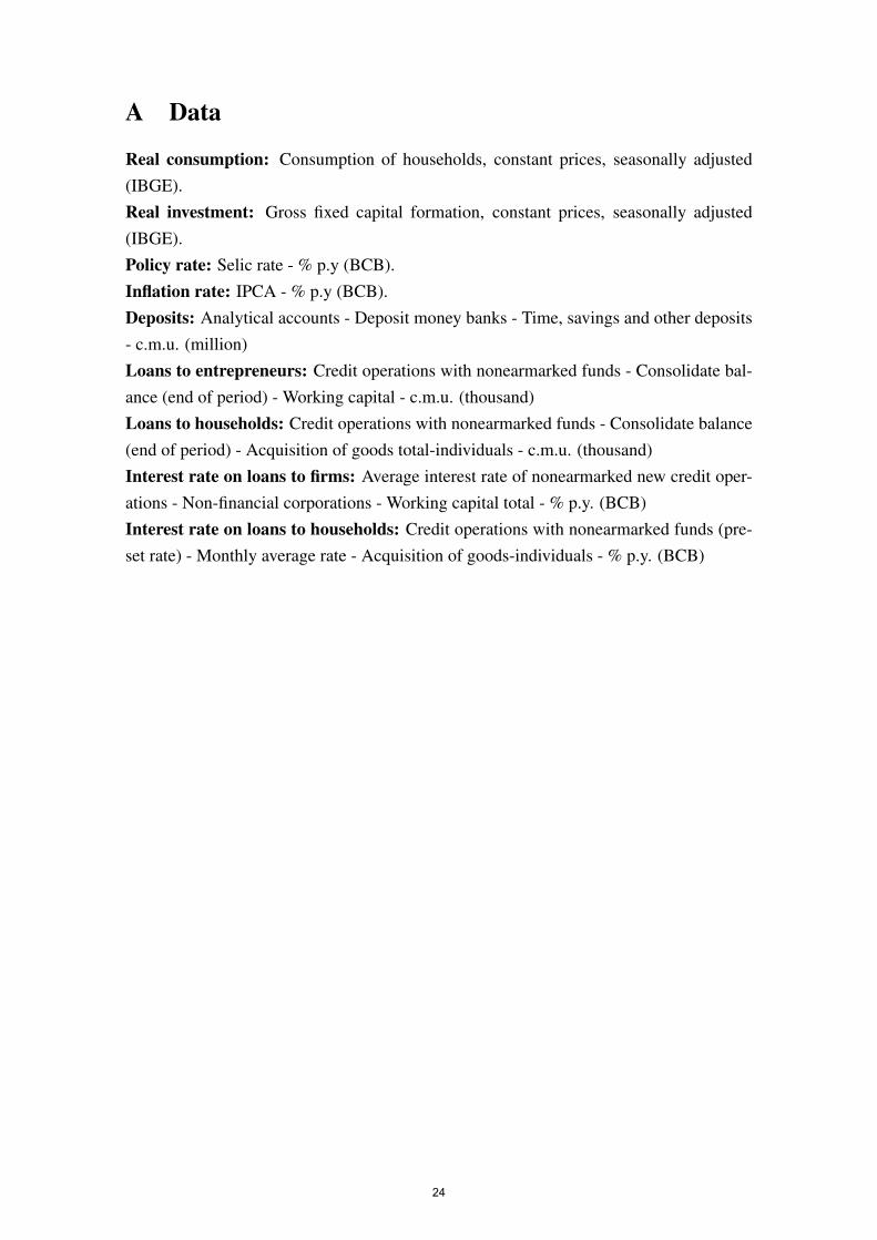
Real consumption: Consumption of households, constant prices, seasonally adjusted(IBGE).Real investment: Gross fixed capital formation, constant prices, seasonally adjusted(IBGE).Policy rate: Selic rate - % p.y (BCB).Inflation rate: IPCA - % p.y (BCB).Deposits: Analytical accounts - Deposit money banks - Time, savings and other deposits- c.m.u. (million)Loans to entrepreneurs: Credit operations with nonearmarked funds - Consolidate bal-ance (end of period) - Working capital - c.m.u. (thousand)Loans to households: Credit operations with nonearmarked funds - Consolidate balance(end of period) - Acquisition of goods total-individuals - c.m.u. (thousand)Interest rate on loans to firms: Average interest rate of nonearmarked new credit oper-ations - Non-financial corporations - Working capital total - % p.y. (BCB)Interest rate on loans to households: Credit operations with nonearmarked funds (pre-set rate) - Monthly average rate - Acquisition of goods-individuals - % p.y. (BCB)

24