lesson 1 - introduction to macroeconomics and review …€¦ · lesson 1 - introduction to...

Lesson 1 - Introduction to Macroeconomics and Review of Microeconomics

IMPORTANT NOTE: This lesson contains a lot of Microeconomics review material. It is more material than can be covered in a week. Use this material to help you remember what was learned in Microeconomics.

Acknowledgement: Ed Sexton and Rick Hirschi were the primary authors of the material contained in this lesson.

Section 1 - Introduction to Macroeconomics

What is Macroeconomics?

Macroeconomics is the study of the economy as a whole, as opposed to microeconomics which is the study of individual firms and consumers.

In this course we will study total output, total levels of employment, total income, aggregate expenditures, the general price level, etc. Do you see the difference between that and studying the output of an individual firm, spending on a single product, or individual price or wage determination?

During our study of macroeconomics we will employ three different levels of analysis: Descriptive Economics, Eco-nomic Theory, and Economic Policy. This course relies heavily on data relevant to the economy. Descriptive Eco-nomics involves the gathering of facts and data that describe the state of the economy. Labor market data, output data, price data, and others will help us understand what is happening in the economy as a whole. Much of this data will allow us to make positive statements about the economy. A positive statement is defined to be a statement of fact. If we gather data on the number of people in the labor force who are unemployed and calculate the unemploy-ment rate to be 8.6%, then the statement, "The unemployment rate is 8.6%" is a positive statement because it is a simple statement of fact.

Economic policy is used to try to manipulate the economy to achieve desired outcomes. Policies are generally designed to meet some goal or target. Typical goals are such things as low employment, price level stability, eco-nomic growth, or balanced trade. Since not everyone would agree what are the most important economic goals to achieve, economic policy almost always involves some value judgment and results in the formulation of normative statements. A normative statement is a statement of what "should be," or a statement of opinion. Therefore, "An unemployment rate of 8.6% is too high, and we should pursue policies to lower the unemployment rate," would be a normative statement.

To a much larger degree than microeconomics, macroeconomics will involve discussions of policies and normative issues about which we may not all agree. Make sure you understand Descriptive Economics and can properly ana-lyze and calculate the various measures that this course will require of you. Also, make sure that you understand the different Economic Theories that are presented in this course. When it comes to Economic Policy, you will have to understand the impact on the economy of various fiscal, monetary, and trade policies, but that will not mean that you have to agree with the Instructor or your fellow students about which of the policies would be best to peruse.

Section 2 - Microeconomics Review - Key Terms

The Economic Perspective

Economics is a Social Science. We study how people and institutions behave given certain constraints. Our behavior is generally directed toward satisfying some want. In fact, we have unlimited wants. The constraint we all face is scarcity. For example, the factors of production are scarce. Land, Labor, Capital, and Entrepreneurship are the factors of production. The payments to these factors are rent, wages, interest, and profit, respectively.

The one fact that none of us can avoid is: to have more of one thing, you'll have to settle for less of another. We are all faced with choices. Every time you make a choice, you incur a cost. The opportunity cost of any action is the best alternative foregone. For example, let's say that you have $50.00 and that you would really like to buy the domain name for an idea that you have. If you do not purchase it right away, there is a danger that someone else will grab it up. The domain name purchase would cost exactly fifty dollars, but there is a problem: you need to fill your gas tank on your car, and the gas will also cost $50.00. Since your resources are scarce (you only have $50.00) what would you choose to buy?

Let's say that you decide to buy the gas. What did the gas cost you? An accountant might say that it cost you $50.00, but an economist would say that it cost you $50.00 and the domain name. The domain name was the opportunity cost of buying the gas. Many choices entail both opportunity costs and explicit or out-of-pocket costs. For example, attending college requires out of pocket costs like tuition, books and fees, but the opportunity costs, your foregone earnings, are probably much greater!

The Assumption of Rationality

We always assume that individuals and all economic entities make decisions based on rational self-interest. Of course, this does not imply that everyone makes the same decision, because different people have different prefer-ences and different levels of utility from consuming. Since we cannot compare the level of utility (satisfaction) from one person to another, we also cannot same someone is irrational if they are acting in a manner that maximizes their utility. A perfectly rational person could choose vanilla ice cream even when chocolate is available, even though someone who likes chocolate may think that decision is irrational! Rationality does not require that we all make the same decisions. Rational self-interest also does not require us to be selfish. The fact that people will behave ratio-nally to advance their self-interests does not preclude altruism or charity. It may be that many, or even most, people have a preference to help those in need when they can. If I feel better when I am being of service to others, then it is in my self-interest to use part of my resources to help others. This helps to explain why members of the church give so freely to the fast offering funds and to humanitarian causes.

Marginal Benefits and Costs

Most of our analysis in economics is marginal analysis. The word "marginal" means incremental or additional. Most decision-making in economics is done on the margin. For example, let's say that Rexburg City is trying to decide whether they should widen a currently two-lane road into a four-lane road. What process will they employ to deter-mine if it is a wise decision? An economist would suggest that the proper criterion would be to compare the marginal benefit and the marginal cost. The marginal benefit would take into account the benefit to the community of having the extra lane going each way. The two lanes that already exist, therefore, are not included in the marginal benefit. The marginal cost would look at the cost of constructing the additional lanes, the additional maintenance costs for maintaining two extra lanes, and the opportunity cost of using the land for a wider road compared to its best alterna-tive use. If the marginal benefit is greater than the marginal cost then the project makes sense. If the marginal cost is greater than the marginal benefit then the city should forgo the project.

Marginal analysis is widely used in many fields of economics and is a concept with which the student of economics

2 Lesson 1 - ECO 151- Master.nb

should become very familiar.

Economic Models

What is a model? A model is a simplified representation of a complex idea or entity. A model airplane is a scaled version of a real airplane, but the model is not necessarily an exact replica of a real airplane. The model gives us a good idea of reality without all of the complexity. Economic models are similar in that they are generally a simplified version of a complex reality. This idea of simplification gives us the primary reason for why economists use models.

Consider the example of a map. Think of a road map as a model. If you were unfamiliar with Los Angeles and were planning to go there on a trip, how would you feel if I gave you a map of Los Angeles exactly the size of Los Ange-les? Would it be helpful to you? No, it would not. If you do not know LA, a map the size of the city would be just as confusing for you as having no map at all. You need the map to be scaled down. The actual economy is much too grand to be studied in detail. We must model the economy to be able to make sense of it. As we study various economic models, it is not helpful for you to think, "But that isn't the way it is in real life!" Generally, economists recognize that they are making simplifying assumptions that are not always true to life, but studying a model that is scaled down is infinitely easier than studying the real thing.

Section 3 - Microeconomics Review - Models of Production

The Circular Flow Model

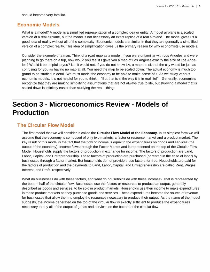
The first model that we will consider is called the Circular Flow Model of the Economy. In its simplest form we will assume that the economy is composed of only two markets: a factor or resource market and a product market. The key result of this model is the fact that the flow of income is equal to the expenditures on goods and services (the output of the economy). Income flows through the Factor Market and is represented on the top of the Circular Flow Model. Households supply the factors of production in exchange for income. The factors of production are Land, Labor, Capital, and Entrepreneurship. These factors of production are purchased (or rented in the case of labor) by businesses through a factor market. But households do not provide these factors for free. Households are paid for the factors of production and the payments to Land, Labor, Capital, and Entrepreneurship are called Rent, Wages, Interest, and Profit, respectively.

What do businesses do with these factors, and what do households do with these incomes? That is represented by the bottom half of the circular flow. Businesses use the factors or resources to produce an output, generally described as goods and services, to be sold in product markets. Households use their income to make expenditures in these product markets as they purchase goods and services. These expenditures become the source of revenue for businesses that allow them to employ the resources necessary to produce their output. As the name of the model suggests, the income generated on the top of the circular flow is exactly sufficient to produce the expenditures necessary to buy all of the output of goods and services on the bottom of the circular flow.

Lesson 1 - ECO 151- Master.nb 3

Circular Flow Model of a Market EconomyThe graphic below shows the circular flow model of a market economy.

Students will often note that the model does not account for the banking sector, the government, foreign trade, etc., suggesting that the model is too simplistic to represent the real economy. Each of these objections could be handled by the circular flow model, but the model would just get more complicated. Remember the more the model resembles the true economy, the more you are trying to navigate an unfamiliar city with an enormously detailed map!

The Production Process

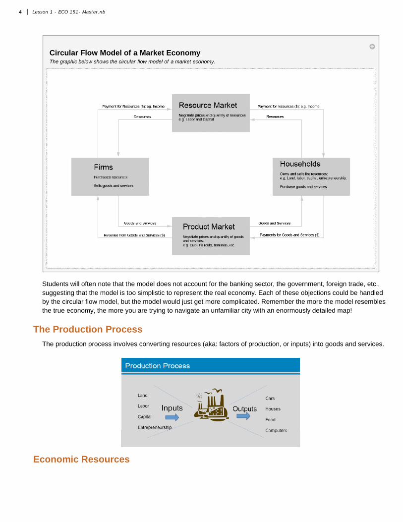
The production process involves converting resources (aka: factors of production, or inputs) into goods and services.

Economic Resources


There are four main categories of resources: land, labor, capital and entrepreneurship.

1. Land

All natural resources both above and below the ground are part of the land resource including farm land, animals, forests, water, minerals, and air. For the use of these resources, businesses pay a rental income.

2. Labor

The labor resource includes both the physical and mental contribution of a worker. As a return for the use of their labor, workers are paid a wage. Education and job training increase human capital or the productivity of the labor resource and thus increase wages – as we'll see later in the course.

3. Capital

Capital includes man-made items that enhance the productivity of labor such as buildings, machinery, and equipment as well as roads and irrigation canals. Unlike consumer goods that directly satisfy our needs and wants today, capi-tal goods, such as machinery, increase our future productivity which then allow us to produce more of the goods and services we want in the future. Interest income is the return or payment for the use of capital. Note that while money is often called capital, it is not an economic resource but simply enables or facilitates the purchase of one of the resources.

4. Entrepreneurship

The last resource is entrepreneurship. Entrepreneurs take risks and combine the other resources to provide goods or services. They are rewarded with profits when their ideas are successful, and suffer the losses when they fail.

All resources or factors of production can be categorized into one of these four resources.

Production Possibility Curves

Another useful model is the model of production. This model helps us explain several important economic concepts, involving trade-offs, that firms face in deciding among production alternatives. There are four simplifying assumptions that we will make in this model:

1. Full Employment—We assume that all of the factors of production are fully employed. We will explore later what would happen in the model if there were unemployed resources.

2. Fixed Resources that are Allocated Efficiently—We assume that at any given point in time, the amount of resources available to the economy is fixed and that these resources are being employed in such a way that there is no way to reallocate the resources and achieve a higher output. In other words, this is an assumption that we are at our maximum output.

3. Fixed Technology—We assume that at any given point in time the technology available to the economy is fixed and that we are using all of our technology to its full potential.


4. Only Two Products are Being Produced—In order to easily represent this model in a two-dimensional plane, we will assume that only two products are being produced in our economy. Given our previous assumptions, this will require that to produce more of one good we must give up production of the other good. The cost of one good in terms of the other good will represent the opportunity cost of production.

Production in a Two-Good Economy

Deriving Production Possibilities Curve PPCThe Production Possibilties Curve PPC is derived from the different combinations of computer programs

and houses we can produce. Those combinations are in the table on the left. When we are producing

at a point such as point B on the production possibilities curve we assume that technology is fixed, that

our resources are fixed, that we are fully using all our resources, and that there is production efficiency

which means we are unable to produce more of one good without producing less of the other goods.

The opportunity cost is the amount sacrificed of the other good to produce one more unit of the good. The marginal

opportunity cost is calculated as follows: What is SacrificedWhat is Gained.

Production Possibilities

Programs Houses

A 0 20B 2 18C 4 14D 6 8E 8 0

Marginal Opp. Costs

Programs Houses

A -- 1 P

B 1 H 12 P

C 2 H 13 P

D 3 H 14 P

E 4 H --

Original source code for graph above from Javier Puertolas. Modified by David Barrus.

Marginal Opportunity Cost

The production possibilities curve also reflects opportunity costs, since to get more of one good we have to sacrifice some of the other. The marginal opportunity cost measures the amount of a good that has to be sacrificed for each additional unit of the other good.

When everyone is working on houses we can produce 20 houses annually (point A). If we wanted 2 computer pro-grams we would have to sacrifice 2 houses as we move from point A to point B. Thus the marginal opportunity cost would be 1 house for each additional computer program. Which individuals would want to move from construction to programming? Likely those individuals who are good at programming and not very good at building houses.

If we wanted an additional 2 computer programs (move from point B to C), we would have to sacrifice 4 houses or 2 houses for each additional program. Note that the marginal opportunity cost is increasing.


As we want more and more computer programs the number of houses we have to sacrifice per computer program increases. As we want more programs, the marginal opportunity cost increases to 2, then 3, and finally as we move from point D to E, we must sacrifice 4 houses for each additional computer program. The increasing marginal opportu-nity cost is due to the fact that some resources are better suited for producing one good than another. Eventually, we have to take experienced construction workers and set them down behind a computer and tell them to start program-ming.

Going the opposite direction, we can compute the marginal opportunity cost for one more house. If we were produc-ing 8 software programs and wanted some housing, we would have to give up 2 computer programs to gain 8 houses, moving from point E to D. Thus a marginal opportunity cost would be 1/4 of a software program per house. As we want more houses, the number of computer programs we would have to sacrifice per house would increase from 1/4 (E to D) to 1/3 (D to C), 1/2 (C to B) and 1 (B to A). For simplicity, we assume that we have to produce at one of the points A through E. Note that as we produce more houses the marginal opportunity costs increases.

Shifts and Movements Along the Production Possibilities Curve

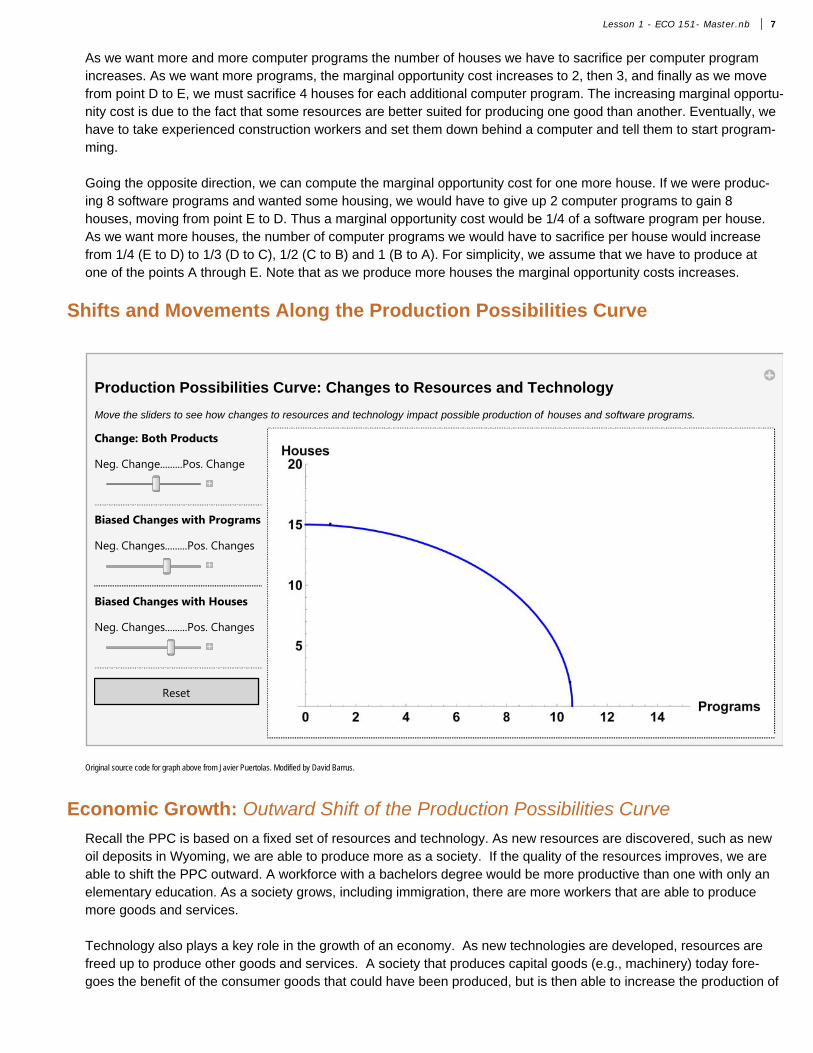
Production Possibilities Curve: Changes to Resources and Technology

Move the sliders to see how changes to resources and technology impact possible production of houses and software programs.

Change: Both Products

Neg. Change.........Pos. Change

Biased Changes with Programs

Neg. Changes.........Pos. Changes

Biased Changes with Houses

Neg. Changes.........Pos. Changes

Reset


Economic Growth: Outward Shift of the Production Possibilities Curve

Recall the PPC is based on a fixed set of resources and technology. As new resources are discovered, such as new oil deposits in Wyoming, we are able to produce more as a society. If the quality of the resources improves, we are able to shift the PPC outward. A workforce with a bachelors degree would be more productive than one with only an elementary education. As a society grows, including immigration, there are more workers that are able to produce more goods and services.

Technology also plays a key role in the growth of an economy. As new technologies are developed, resources are freed up to produce other goods and services. A society that produces capital goods (e.g., machinery) today fore-goes the benefit of the consumer goods that could have been produced, but is then able to increase the production of


goods and services in the future due to the machinery and other improvements that have been made. In 1950, one farmer in the U.S. fed 15 other people. By 1995, that number had increased to 128 and continues to rise. As technol-ogy advances and farmers use more and more capital, not as many people are required to be in agriculture and are able to go produce cars, TVs, and other goods and services that we enjoy. (Reference: Agriculture, Technology and the Economy Agriculture, Technology and the Economy Federal Reserve Bank of Dallas: http://www.dallasfed.org/re-search/pubs/agtech.html)

Inward Shift of the Production Possibilities Curve

If a society loses resources, the production possibilities curve would shift in. The loss of resources may come about from war, natural disasters, such as earthquakes or hurricanes, or disease, such as AIDS.

Biased Technologies: Partial Shift of the Production Possibilities Curve

Biased technologies only impact the production of one good. For example, the printing press allowed for more books to be produced, but didn't increase the number of wagons (if all resources were devoted to wagon production). When both goods are being produced, a biased technology reduces the number of resources being required to produce that good, so more of the resources can be devoted to producing the other good.

Graphically, if a nail gun is invented then it would cause a shift in the production possibilities curve only for the production of houses and not for the production of programs. This would cause a shift outward of the production possibility only on the axis for houses.

Production Possibilities Curve: Movements

Move the sliders to see movements along the PPC, location of inefficient and unattainable points.

Marginal opportunity costs are calculated from point A as you move along the PPC.

Movement Along PPC

More Houses.....................................More Programs

Movement Away from PPC

Inefficient..............Efficient...............Unattainable

Marginal Opp. CostsThe marginal opp. cost between the two points

on the PPCPoint A = 10 programs, 5 housesPoint D = 10 programs 5 housesMOC of 1 more house = 0. programsMOC of 1 more program = 0. houses

Reset


Movements Away from the Production Possibilities Curve

If the resources or technology of a society change, the PPC will shift in or out. However, the PPC does not shift when resources are left unused or when they are not used efficiently. In this latter case, production would simply be illus-


trated by a point inside the PPC, i.e. society would be moving away from the PPC to an interior point. For example, an increase in the unemployment rate would move a society further inside the PPC. Note that the resources still exist so the PPC has not changed, we are just not using all of resources that we have. Move the slider "Movement Away from PPC" to see an inefficient point and an unattainable point.

Moving Toward the Production Possibilities Curve

Conversely, if more unused resources are used or the resources are used more efficiently (not due to a change in technology), the society would move toward the PPC.

Moving Along the Productions Possibilities Curve

Movement along the PPC occurs when there is a change in the combination of goods and services produced. In a market economy, consumers signal to producers the types of goods and services they desire and are willing to pay for. Use to slider on the graph above to see a movement along the PPC. Notice how the marginal opportunity costs change as the point moves.

Section 4: Microeconomics Review - Supply and Demand

The Law of Demand

A market brings together and facilitates trade between buyers and sellers of goods or services. These markets range from bartering in street markets to trades that are made through the Internet with individuals, around the world, that never have met face to face.

A market consists of those individuals who are willing and able to purchase the particular good and sellers who are willing and able to supply the good. The market brings together those who demand and supply the good to determine the price.

For example, the number of many apples an individual would be willing and able to buy each month depends in part on the price of apples. Assuming only price changes, then at lower prices, a consumer is willing and able to buy more apples. As the price rises (again holding all else constant), the quantity of apples demanded decreases. The Law of Demand captures this relationship between price and the quantity demanded of a product. It states that there is an inverse (or negative) relationship between the price of a good and the quantity demanded.


Downward Sloping Demand for Apples

As the price of apples increase, the quantity demanded decreases. This is because consumers demand less

at a higher price. As the price of apples decreases,the quantity demanded increases since consumers demand

more at a lower price. This is the law of demand.

Table for Demand

Price No. of Apples

5 3010 2515 2220 1825 1530 1235 1040 5

Pri

ce

Quantity Demanded of Apples

Original source code for graph above from Javier Puertolas. Modified by David Barrus and Victoria Cole.

Demand Curve

Recall, that we represent economic laws and theory using models; in this case we can use a demand schedule or a demand curve to illustrate the Law of Demand. The demand schedule shows the combinations of price and quantity demanded of apples in a table format. The graphical representation of the demand schedule is called the demand curve.

When graphing the demand curve, price goes on the vertical axis and quantity demanded goes on the horizontal axis. A helpful hint when labeling the axes is to remember that since P is a tall letter, it goes on the vertical axis. Another hint when graphing the demand curve is to remember that demand descends.

Rationales for the Law of Demand

Below are listed four rationales for why the demand curve has a downward slope. The first is what might be called the man on the street explanation. It is just the logical description of how most people behave. The other three rationales rely on economic principles.

1. People buy more of a given product at lower prices than they do at higher prices.

2. In any given time period, a buyer of a product will derive less utility from each successive unit of a product he consumes. This is called diminishing marginal utility. Since a consumer is receiving less utility from each additional unit of a good consumed, he will only buy successive units at lower prices.

3. Income Effect of a Price Change—At lower prices, one can afford to buy more of all goods, because one's income stretches further. Thus, at lower prices higher quantities are demanded. The reverse is also true.

4. Substitution Effect of a Price Change—As the price of a good falls you tend to substitute away from higher priced good and buy more of this relatively cheaper good. As the price of good "A" falls the quantity demanded for


good "A" goes up because it is relatively cheaper than other goods for which prices remained constant.

At this point, we have explained why there is an inverse relationship between price and quantity demanded (i.e. we've explained the law of demand). The changes in price that we have discussed cause movements along the demand curve, called changes in quantity demanded. But there are factors other than price that cause complete shifts in the demand curve which are called changes in demand (Note: These new factors also determine the actual placement of the demand curve on a graph).

Factors that Shift the Demand Curve

While a change in the price of the good moves us along the demand curve to a different quantity demanded, a change or shift in demand will cause a different quantity demanded at each and every price. A rightward shift in demand would increase the quantity demanded at all prices compared to the original demand curve. For example, at a price of $40, the quantity demanded would increase from 40 units to 60 units. A helpful hint to remember that more demand shifts the demand curve to the right. Move the slider on the graph below to see the rightward shift.

A leftward shift in demand would decrease the quantity demanded to 20 units at the price of $40. With a decrease in demand, there is a lower quantity demanded at each an every price along the demand curve. Move the slider on the graph below to see the leftward shift. The factors that cause shifts in demand are discussed below.

Demand Curve Shifts

Use the slider bar to shift the demand curve from left to right.

Shifts in the Demand Curve

Left.................................Right

Factors that Cause Demand to Shift

1. Changes in Tastes & Preferences2. Changes in Prices of Related Goods3. Changes in Income4. Expectations of the Future5. Number of Buyers

Reset


1. Change in Tastes and Preferences

A change in tastes and preferences will cause the demand curve to shift either to the right or left. For example, if new research found that eating apples increases life expectancy and reduces illness, then more apples would be pur-chased at each and every price causing the demand curve to shift to the right. Companies spend billions of dollars in advertising to try and change individuals' tastes and preferences for a product. Celebrities or sports stars are often hired to endorse a product to increase the demand for a product. A leftward shift in demand is caused by a factor that adversely effects the tastes and preferences for the good. For example, if a pesticide used on apples is shown to have adverse health effects.


2. Changes in Prices of Related Goods

Another factor that determines the demand for a good is the price of related goods. These can be broken down into two categories – substitutes and complements. A substitute is something that takes the place of the good. Instead of buying an apple, one could buy an orange. If the price of oranges goes up, we would expect an increase in demand for apples since consumers would move consumption away from the higher priced oranges towards apples which might be considered a substitute good. Complements, on the other hand, are goods that are consumed together, such as caramels and apples. If the price for a good increases, its quantity demanded will decrease and the demand for the complements of that good will also decline. For example, if the price of hot dogs increases, one will buy fewer hot dogs and therefore demand fewer hot dog buns, which are complements to hot dogs.

3. Changes in Income

Remember that demand is made up of those who are willing and able to purchase the good at a particular price. Income influences both willingness and ability to pay. As one's income increases, a person's ability to purchase a good increases, but she/he may not necessarily want more. If the demand for the good increases as income rises, the good is considered to be a normal good. Most goods fall into this category; we want more cars, more TVs, more boats as our income increases. As our income falls, we also demand fewer of these goods. Inferior goods have an inverse relationship with income. As income rises we demand fewer of these goods, but as income falls we demand more of these goods. Although individual preferences influence if a good is normal or inferior, in general, Top Ramen, Mac and Cheese, and used clothing fall into the category of an inferior good.

4. Expectations of the Future

Another factor of demand is future expectations. This includes expectations of future prices and income. An individ-ual that is graduating at the end of the semester, who has just accepted a well paying job, may spend more today given the expectation of a higher future income. This is especially true if the job offer is for more income than what he had originally anticipated. If one expects the price of apples to go up next week, she will likely buy more apples today while the price is still low.

5. Number of Buyers

The last factor of demand is the number of buyers. A competitive market is made up of many buyers and many sellers. Thus a producer is not particularly concerned with the demand of one individual but rather the demand of all the buyers collectively in that market. As the number of buyers increases or decreases, the demand for the good will change.

Demand vs. Quantity Demanded

At this point, it is important to re-emphasize that there is an important distinction between changes in demand and changes in quantity demanded. The entire curve showing the various combinations of price and quantity demanded represents the demand curve. Thus a change in the price of the good does not shift the curve (or change demand) but causes a movement along the demand curve to a different quantity demanded. If the price returned to its original price, we would return to the original quantity demanded.


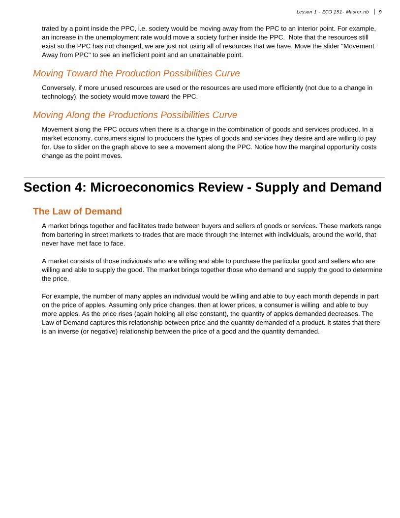
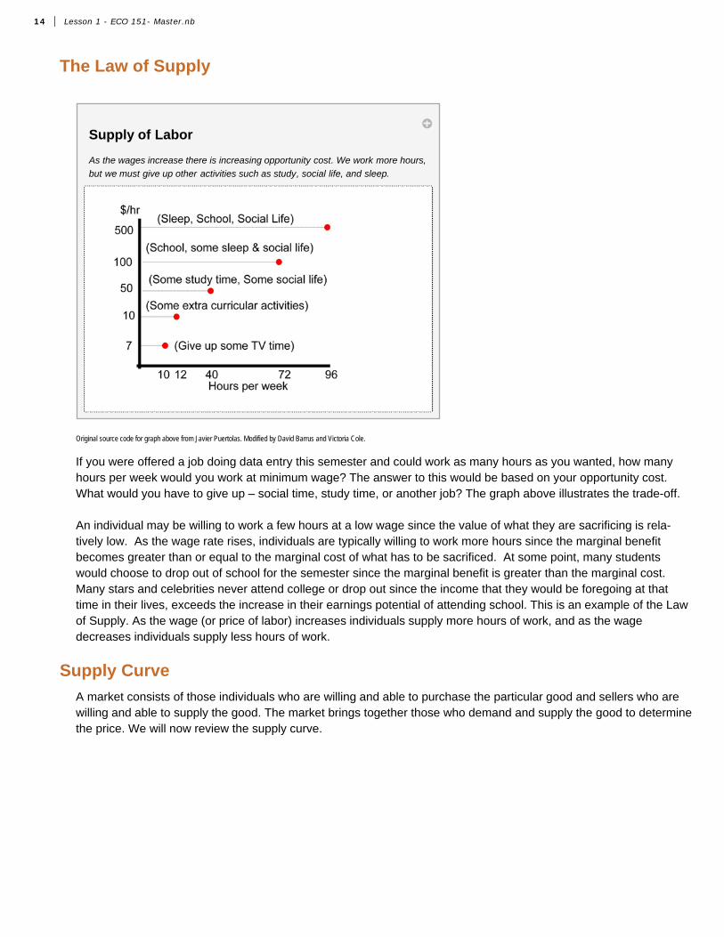
Demand Curve Shifts vs. Movements Along the Demand Curve

Use the first slider bar to shift the demand curve from left to right, and the second slider bar to change the price of the good.


Left...................................................................Right

Factors that Cause Demand to Shift1. Changes in Tastes & Preferences2. Changes in Prices of Related Goods3. Changes in Income4. Expectations of the Future5. Number of Buyers

Movements along Demand CurveDecrease in Price..................Increase in Price

Price Change =Movement along curve1. P increases, Qd decreases1. P decreases, Qd increases

Reset


If the price were originally $40, the quantity demanded would be 40 units. An increase in the price of the good to $60 decreases the quantity demanded to 20 units. This is a movement along the demand curve to a new quantity demanded. Note that if the price were to return to $40, the quantity demanded would also return to the 40 units. Move the second slider in the graph above to see this movement.

A shift or change in demand comes about when there is a different quantity demanded at each price. At $40 we originally demanded 40 units. If there is a lower quantity demanded at each price, the demand curve has shifted left. Now at $40, there are only 20 units demanded. Shift the top or first slider in the graph above to see this shift. Shifts in demand are caused by factors other than the price of the good and, as discussed, include changes in: 1) tastes and preferences; 2) price of related goods; 3) income; 4) expectations about the future; and 5) market size.


The Law of Supply

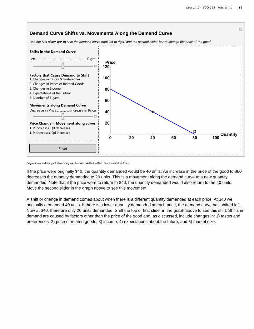
Supply of Labor

As the wages increase there is increasing opportunity cost. We work more hours,

but we must give up other activities such as study, social life, and sleep.


If you were offered a job doing data entry this semester and could work as many hours as you wanted, how many hours per week would you work at minimum wage? The answer to this would be based on your opportunity cost. What would you have to give up – social time, study time, or another job? The graph above illustrates the trade-off.

An individual may be willing to work a few hours at a low wage since the value of what they are sacrificing is rela-tively low. As the wage rate rises, individuals are typically willing to work more hours since the marginal benefit becomes greater than or equal to the marginal cost of what has to be sacrificed. At some point, many students would choose to drop out of school for the semester since the marginal benefit is greater than the marginal cost. Many stars and celebrities never attend college or drop out since the income that they would be foregoing at that time in their lives, exceeds the increase in their earnings potential of attending school. This is an example of the Law of Supply. As the wage (or price of labor) increases individuals supply more hours of work, and as the wage decreases individuals supply less hours of work.

Supply Curve

A market consists of those individuals who are willing and able to purchase the particular good and sellers who are willing and able to supply the good. The market brings together those who demand and supply the good to determine the price. We will now review the supply curve.


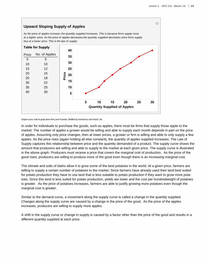
Upward Sloping Supply of Apples

As the price of apples increase, the quantity supplied increases. This is because firms supply more

at a higher price. As the price of apples decreases,the quantity supplied decreases since firms supply

less at a lower price. This is the law of supply.

Table for Supply

Price No. of Apples

5 5

10 1015 1220 1525 1830 2235 2540 30

Pri

ce

Quantity Supplied of Apples


In order for individuals to purchase the goods, such as apples, there must be firms that supply those apple to the market. The number of apples a grower would be willing and able to supply each month depends in part on the price of apples. Assuming only price changes, then at lower prices, a grower or firm is willing and able to only supply a few apples. As the price rises (again holding all else constant), the quantity of apples supplied increases. The Law of Supply captures this relationship between price and the quantity demanded of a product. The supply curve shows the amount that producers are willing and able to supply to the market at each given price. The supply curve is illustrated in the above graph. Producers must receive a price that covers the marginal cost of production. As the price of the good rises, producers are willing to produce more of the good even though there is an increasing marginal cost.

The climate and soils of Idaho allow it to grow some of the best potatoes in the world. At a given price, farmers are willing to supply a certain number of potatoes to the market. Since farmers have already used their land best suited for potato production they have to use land that is less suitable to potato production if they want to grow more pota-toes. Since this land is less suited for potato production, yields are lower and the cost per hundredweight of potatoes is greater. As the price of potatoes increases, farmers are able to justify growing more potatoes even though the marginal cost is greater.

Similar to the demand curve, a movement along the supply curve is called a change in the quantity supplied. Changes along the supply curve are caused by a change in the price of the good. As the price of the apples increases, producers are willing to supply more apples.

A shift in the supply curve or change in supply is caused by a factor other than the price of the good and results in a different quantity supplied at each price.


Factors that Shift the Supply Curve

Supply Curve Shifts

Use the slider bar to shift the supply curve from left to right.

Shifts in the Supply Curve

Left.................................Right

Factors that Cause Demand to Shift

1. Changes in Resource Prices2. Changes in Technique of Production3. Changes in Prices of Other Goods4. Changes in Taxes & Subsidies5. Expectations of Future Prices6. Number of Sellers7. Supply Shocks

Reset


The factors listed below will shift the supply curve either to the right or to the left.

1. Changes in Resource Prices

If the price of crude oil (a resource or input into gasoline production) increases, the quantity supplied of gasoline at each price would decline, shifting the supply curve to the left.

2. Changes in Technique of Production

If a new method or technique of production is developed, the cost of producing each good declines and producers are willing to supply more at each price - shifting the supply curve to the right.

3. Changes in Prices of Other Goods

If the price of wheat increases relative to the price of other crops that could be grown on the same land, such as potatoes or corn, then producers will want to grow more wheat, ceteris paribus. By increasing the resources devoted to growing wheat, the supply of other crops will decline. Goods that are produced using similar resources are substi-tutes in production.

Complements in production are goods that are jointly produced. Beef cows provide not only steaks and hamburger but also leather that is used to make belts and shoes. An increase in the price of steaks will cause an increase in the quantity supplied of steaks and will also cause an increase (or shift right) in the supply of leather which is a comple-ment in production.

4. Changes in Taxes & Subsidies


Taxes and subsidies impact the profitability of producing a good. If businesses have to pay more taxes, the supply curve would shift to the left. On the other hand, if businesses received a subsidy for producing a good, they would be willing to supply more of the good, thus shifting the supply curve to the right.

5. Expectation of Future Prices

Expectations about the future price will shift the supply. If sellers anticipate that home values will decrease in the future, they may choose to put their house on the market today before the price falls. Unfortunately, these expecta-tions often become self-fulfilling prophecies, since if many people think values are going down and put their house on the market today, the increase in supply leads to a lower price.

6. Number of sellers

If more companies start to make motorcycles, the supply of motorcycles would increase. If a motorcycle company goes out of business, the supply of motorcycles would decline, shifting the supply curve to the left.

7. Supply Shocks

The last factor is often out of the hands of the producer. Natural disasters such as earthquakes, hurricanes, and floods impact both the production and distribution of goods. While supply shocks are typically negative, there can be beneficial supply shocks with rains coming at the ideal times in a growing season.

Supply vs. Quantity Supplied

To recap, changes in the price of a good will result in movements along the supply curve called changes in quantity supplied. Move the second or bottom slider to see the movements along the supply curve (changes in quantity supplied). A change in any of the other factors we've discussed (and listed above), will shift the supply curve either right or left. The resulting movements are called changes in supply. Move the top or first slider on the graph above to see the curve shift to the right or left.


Supply Curve Shifts vs. Movements Along the Supply Curve

Use the first slider bar to shift the supply curve from left to right, and the second slider bar to change the price of the good.


Left...................................................................Right

Factors that Cause Supply to Shift

1. Changes in Resource Prices2. Changes in Technique of Production3. Changes in Prices of Other Goods4. Changes in Taxes & Subsidies5. Expectations of Future Prices6. Number of Sellers7. Supply Shocks

Movements along Supply CurveDecrease in Price..................Increase in Price

Price Change =Movement along curve1. P increases, Qs increases1. P decreases, Qs decreases

Reset


Market Equilibrium

A market brings together those who are willing and able to supply the good and those who are willing and able to purchase the good. In a competitive market, where there are many buyers and sellers, the price of the good serves as a rationing mechanism. Since the demand curve shows the quantity demanded at each price and the supply curve shows the quantity supplied, the point at which the supply curve and demand curve intersect is the point at where the quantity supplied equals the quantity demanded. This is call the market equilibrium. In the graph above it is where the price is $40 and the quantity is 40.


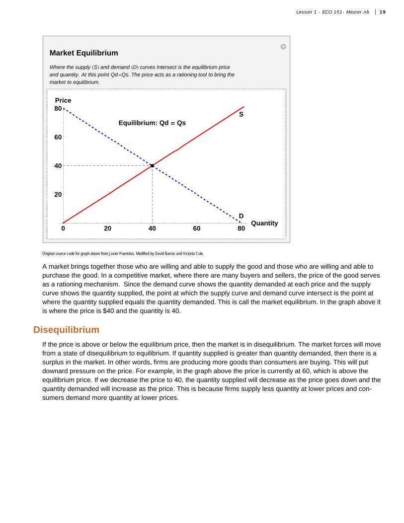
Market Equilibrium

Where the supply S and demand D curves intersect is the equilibrium price

and quantity. At this point Qd=Qs. The price acts as a rationing tool to bring the

market to equilibrium.

D

SEquilibrium: Qd = Qs

0 20 40 60 80Quantity

20

40

60

80Price


A market brings together those who are willing and able to supply the good and those who are willing and able to purchase the good. In a competitive market, where there are many buyers and sellers, the price of the good serves as a rationing mechanism. Since the demand curve shows the quantity demanded at each price and the supply curve shows the quantity supplied, the point at which the supply curve and demand curve intersect is the point at where the quantity supplied equals the quantity demanded. This is call the market equilibrium. In the graph above it is where the price is $40 and the quantity is 40.

Disequilibrium

If the price is above or below the equilibrium price, then the market is in disequilibrium. The market forces will move from a state of disequilibrium to equilibrium. If quantity supplied is greater than quantity demanded, then there is a surplus in the market. In other words, firms are producing more goods than consumers are buying. This will put downard pressure on the price. For example, in the graph above the price is currently at 60, which is above the equilibrium price. If we decrease the price to 40, the quantity supplied will decrease as the price goes down and the quantity demanded will increase as the price. This is because firms supply less quantity at lower prices and con-sumers demand more quantity at lower prices.


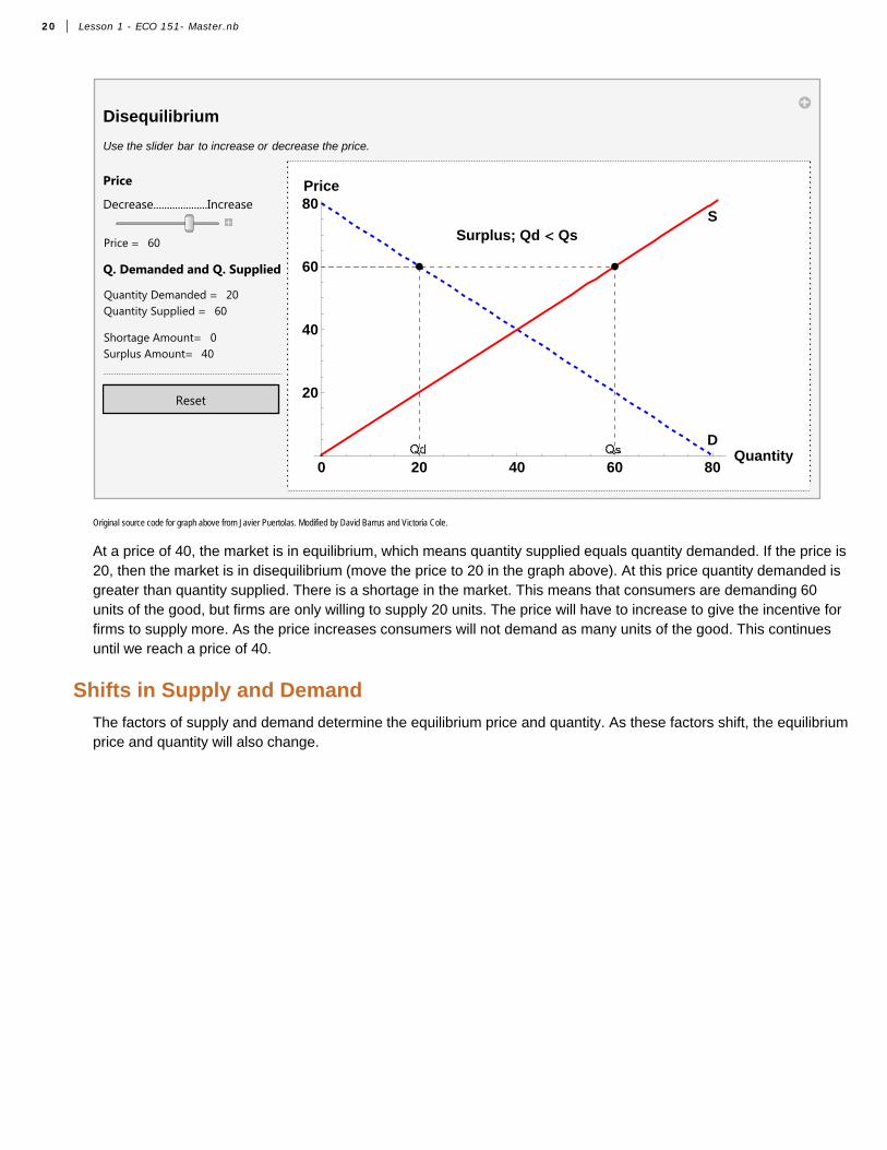
Disequilibrium

Use the slider bar to increase or decrease the price.

Price

Decrease....................Increase

Price = 60

Q. Demanded and Q. Supplied

Quantity Demanded = 20Quantity Supplied = 60

Shortage Amount= 0Surplus Amount= 40

Reset

0 20 40 60 80Quantity

20

40

60

80Price

D

SSurplus; Qd < Qs


At a price of 40, the market is in equilibrium, which means quantity supplied equals quantity demanded. If the price is 20, then the market is in disequilibrium (move the price to 20 in the graph above). At this price quantity demanded is greater than quantity supplied. There is a shortage in the market. This means that consumers are demanding 60 units of the good, but firms are only willing to supply 20 units. The price will have to increase to give the incentive for firms to supply more. As the price increases consumers will not demand as many units of the good. This continues until we reach a price of 40.

Shifts in Supply and Demand

The factors of supply and demand determine the equilibrium price and quantity. As these factors shift, the equilibrium price and quantity will also change.


Demand Curve Shifts

Use the slider bar to shift the demand curve to the left or the right. When demand shifts in or to the left, there is a lower quantity

demanded at each price. When demand shifts out or to the right, there is a higher quantity demanded at each price. Move the

slider to find out what happens to equilibrium price and quantity as the demand curve shifts and supply stays constant.


Left.................................Right

Demand Shifts

Ò Æ or ∞

Eq. Price = 40

Eq. Quantity = 40

Reset


If the demand decreases, for example a particular style of sunglasses becomes less popular, i.e., a change a tastes and preferences, the quantity demanded at each price has decreased. At the current price there is now a surplus in the market and pressure for the price to decrease. The new equilibrium will be at a lower price and lower quantity. Note that the supply curve does not shift but a lower quantity is supplied due to a decrease in the price.

If the demand curve shifts right, there is a greater quantity demanded at each price. The newly created shortage at the original price will drive the market to a higher equilibrium price and quantity. As the demand curve shifts the equilibrium price and quantity will change in the same direction, i.e., both will increase or both will decrease.


Supply Curve Shifts

Use the slider bar to shift the supply curve to the left or the right. When supply shifts in or to the left, there is a lower quantity

supplied at each price. When supply shifts out or to the right, there is a higher quantity supplied at each price. Move the

slider to find out what happens to equilibrium price and quantity as the supply curve shifts and demand stays constant.


Left.................................Right

Supply Shifts

Ò Æ or ∞

Eq. Price = 40

Eq. Quantity = 40

Reset


If the supply curve shifts left, say due to an increase in the price of the resources used to make the product, there is a lower quantity supplied at each price. The result will be an increase in the market equilibrium price but a decrease in the market equilibrium quantity. The increase in price, causes a movement along the demand curve to a lower equilibrium quantity demanded.

A rightward shift in the supply curve, say from a new production technology, leads to a lower equilibrium price and a greater quantity. Note that as the supply curve shifts, the change in the equilibrium price and quantity will be in opposite directions.


Complex Cases - Shifting Supply and Demand

Supply and Demand Curve Shifts - Complex Cases

Use the slider bar to shift the supply and demand curves to the left or the right. Watch what happens to equilibrium price and quantity.

The arrows in the table indicate if the equilibrium price and quantity has increased Æ, decreased ∞, or stayed at the same value õ.


Left.................................Right


Left.................................Right

Ò Æ,∞,õ

Eq. Price = 40. õ

Eq. Quantity = 40. õ

Reset


When demand and supply are changing at the same time, the analysis becomes more complex. In such cases, we are still able to say whether one of the two variables (equilibrium price or quantity) will increase or decrease, but we may not be able to say how both will change. When the shifts in demand and supply are driving price or quantity in opposite directions, we are unable to say how one of the two will change without further information.

Complex Cases - Solving for Equilibrium Algebraically

We are able to find the market equilibrium by analyzing a schedule or table, by graphing the data, or solving equa-tions algebraically. While it is easy to ready a table or look at a graph to find equilibrium, it is harder to algebraically solve for equilibrium. We will review how to solve for equilibrium below.

The data can also be represented by equations.

P = 50 – 2Qd and P = 10 + 2 Qs

Solving the equations algebraically will also enable us to find the point where the quantity supplied equals the quan-tity demanded and the price where that will be true. We do this by setting the two equations equal to each other and solving. The steps for doing this are illustrated below.

As stated above, at equilibrium Qd = Qs = Q. Our first step is to get the Qs together, by adding 2Q to both sides. On the left hand side, the negative 2Q plus 2Q cancel each other out, and on the right side 2 Q plus 2Q gives us 4Q. Our next step is to get the Q by itself. We can subtract 10 from both sides and are left with 40 = 4Q. The last step is to divide both sides by 4, which leaves us with an equilibrium Quantity of 10.

Given an equilibrium quantity of 10, we can plug this value into either the equation we have for supply or demand


and find the equilibrium price of $30. Either graphically or algebraically, we end up with the same answer.

Step-by-Step Solving Algebraically

1. Quantity supplied equals quantity demanded at equilibrium: Qd = Qs = Q (step 1)

2. Set the two equations equal to each other: 50 – 2Q = 10 + 2Q (step 2)

3. Get Qs together. Add 2Q to both sides: 50 - 2Q + 2Q = 10 + 2Q + 2Q (step 3)50 = 10 + 4Q

4. Get Q by itself by subtracting 10 from both sides: 50 - 10 = 10 -10 + 4Q (step 4)40 = 4Q

5. Divide both sides by 4. Solve for eq. quantity = Q*: 40/4 = 4Q/4 (step 5)10 = Q*

6. Plug Q* = 10 back into an equation to get eq. price = P*: P = 50 - 2(10) or P = 10 + 2(10)(step 6)P* = 30 or P* = 30

Section 5: Microeconomics Review - Market InterventionIf a competitive market is free of intervention, market forces will always drive the price and quantity towards the equilibrium. However, there are times when government feels a need to intervene in the market and prevent it from reaching equilibrium. While often done with good intentions, this intervention often brings about undesirable sec-ondary effects. Market intervention often comes as either a price floor or a price ceiling.


Market Intervention - Price Floor

Market Intervention - Price Floor

Use the slider bar to increase or decrease the price floor. A binding price floor is above equilibrium. This means the price

cannot fall below the price floor to equilibrium. If the price floor is below equilibrium, then the price floor

is non-binding because the price can move to equilibrim. Example: Minimum Wage

Price


Price = 60




Reset

0 20 40 60 80Quantity

20

40

60

80Price

D

SPrice Floor: Binding

Surplus Created Qd < Qs


A price floor sets a minimum price for which the good may be sold. Price floors are designed to benefit the produc-ers providing them a price greater than the original market equilibrium. To be effective, a price floor would need to be above the market equilibrium. At a price above the market equilibrium the quantity supplied will exceed the quantity demanded resulting in a surplus in the market.

For example, the government imposed price floors for certain agricultural commodities, such as wheat and corn. At a price floor, greater than the market equilibrium price, producers increase the quantity supplied of the good. However, consumers now face a higher price and reduce the quantity demanded. The result of the price floor is a surplus in the market.

Since producers are unable to sell all of their product at the imposed price floor, they have an incentive to lower the price but cannot. To maintain the price floor, governments are often forced to step in and purchase the excess product, which adds an additional costs to the consumers who are also taxpayers. Thus the consumers suffer from both higher prices but also higher taxes to dispose of the product.

The decision to intervene in the market is a normative decision of policy makers. Is the benefit to those receiving a higher wage greater than the added cost to society? Is the benefit of having excess food production greater than the additional costs that are incurred due to the market intervention?

Another example of a price floor is a minimum wage. In the labor market, the workers supply the labor and the businesses demand the labor. If a minimum wage is implemented that is above the market equilibrium, some of the individuals who were not willing to work at the original market equilibrium wage are now willing to work at the higher wage, i.e., there is an increase in the quantity of labor supplied. Businesses must now pay their workers more and consequently reduce the quantity of labor demanded. The result is a surplus of labor available at the minimum wage.


Due to the government imposed price floor, price is no longer able to serve as the rationing device and individuals who are willing and able to work at or below the going minimum wage may not be able to find employment.

Market Intervention - Price Ceiling

Market Intervention - Price Ceilings

Use the slider bar to increase or decrease the price ceiling. A binding price ceiling is below equilibrium. This means the price

cannot rise above the price ceiling to equilibrium. If the price ceiling is above equilibrium, then the price ceiling

is non-binding because the price can move to equilibrim. Example: Rent Control

Price


Price = 20




Reset

0 20 40 60 80Quantity

20

40

60

80Price

D

SPrice Ceiling: Binding

Shortage Created Qd > Qs


Price ceilings are intended to benefit the consumer, and the government sets a maximum price for which the product may be sold. To be effective, the price ceiling must be below the market equilibrium. Some large metropolitan areas control the price that can be charged for apartment rent. The result is that more individuals want to rent apartments given the lower price, but apartment owners are not willing to supply as many apartments to the market (i.e., a lower quantity supplied). In many cases when price ceilings are implemented, black markets or illegal markets develop that facilitate trade at a price above the set government maximum price.


Impacts of Market Intervention

Market Intervention - Price Ceilings, Price Floors, & Deadweight Loss

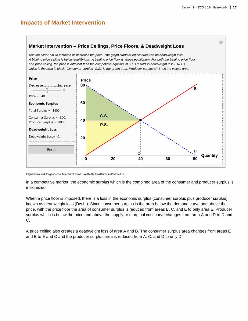
Use the slider bar to increase or decrease the price. The graph starts at equilibrium with no deadweight loss.

A binding price ceiling is below equilibrium. A binding price floor is above equilibrium. For both the binding price floor

and price ceiling, the price is different than the competitive equilibrium. This results in deadweight loss Dw.L.,which is the area in black. Consumer surplus C.S. is the green area. Producer surplus P.S. is the yellow area.

Price


Price = 40

Economic Surplus

Total Surplus = 1600.

Consumer Surplus = 800.Producer Surplus = 800.

Deadweight Loss

Deadweight Loss= 0.

Reset

0 20 40 60 80Quantity

20

40

60

80Price

D

S

C.S.

P.S.


In a competitive market, the economic surplus which is the combined area of the consumer and producer surplus is maximized.

When a price floor is imposed, there is a loss in the economic surplus (consumer surplus plus producer surplus) known as deadweight loss (Dw.L.). Since consumer surplus is the area below the demand curve and above the price, with the price floor the area of consumer surplus is reduced from areas B, C, and E to only area E. Producer surplus which is below the price and above the supply or marginal cost curve changes from area A and D to D and C.

A price ceiling also creates a deadweight loss of area A and B. The consumer surplus area changes from areas E and B to E and C and the producer surplus area is reduced from A, C, and D to only D.


Excise Tax

Market Intervention - Excise Tax, Tax Revenue, & Deadweight Loss

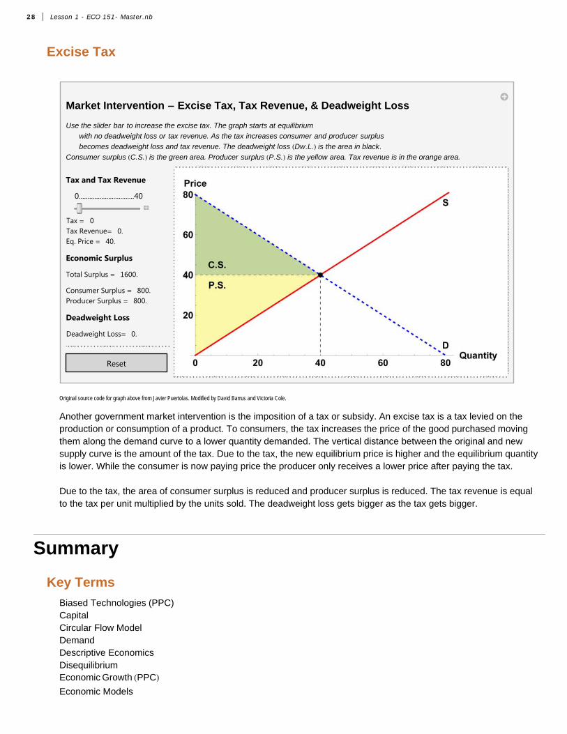
Use the slider bar to increase the excise tax. The graph starts at equilibrium

with no deadweight loss or tax revenue. As the tax increases consumer and producer surplus

becomes deadweight loss and tax revenue. The deadweight loss Dw.L. is the area in black.

Consumer surplus C.S. is the green area. Producer surplus P.S. is the yellow area. Tax revenue is in the orange area.

Tax and Tax Revenue

0................................40

Tax = 0Tax Revenue= 0.Eq. Price = 40.

Economic Surplus

Total Surplus = 1600.

Consumer Surplus = 800.Producer Surplus = 800.

Deadweight Loss

Deadweight Loss= 0.

Reset


Another government market intervention is the imposition of a tax or subsidy. An excise tax is a tax levied on the production or consumption of a product. To consumers, the tax increases the price of the good purchased moving them along the demand curve to a lower quantity demanded. The vertical distance between the original and new supply curve is the amount of the tax. Due to the tax, the new equilibrium price is higher and the equilibrium quantity is lower. While the consumer is now paying price the producer only receives a lower price after paying the tax.

Due to the tax, the area of consumer surplus is reduced and producer surplus is reduced. The tax revenue is equal to the tax per unit multiplied by the units sold. The deadweight loss gets bigger as the tax gets bigger.

Summary

Key Terms

Biased Technologies (PPC)CapitalCircular Flow ModelDemandDescriptive EconomicsDisequilibriumEconomic Growth PPCEconomic Models


Economic PerspectiveEconomic PolicyEconomic ResourcesEconomic TheoriesEntrepreneurshipLaborLandMacroeconomicsMarginal AnalysisMarginal BenefitsMarginal CostsMarginal Opportunity CostMarket EquilibriumMicroeconomicsNormative StatementPositive StatementPrice CeilingPrice FloorProduction Possibility CurvesProduction ProcessRationalitySupply

© 2013 by Brigham Young University-Idaho. All rights reserved.


lesson 1 - introduction to macroeconomics and review …€¦ · lesson 1 - introduction to...

Documents