levenberg-marquardt optimised neural networks for ...sro.sussex.ac.uk/61718/1/ijma0502-0309...
TRANSCRIPT
Levenberg-Marquardt optimised neural networks for trajectory tracking of autonomous ground vehicles
Article (Published Version)
http://sro.sussex.ac.uk
Al-Mayyahi, Auday Basheer Essa, Wang, Weiji and Birch, Philip (2015) Levenberg-Marquardt optimised neural networks for trajectory tracking of autonomous ground vehicles. International Journal of Mechatronics and Automation, 5 (2/3). pp. 140-153. ISSN 2045-1067
This version is available from Sussex Research Online: http://sro.sussex.ac.uk/61718/
This document is made available in accordance with publisher policies and may differ from the published version or from the version of record. If you wish to cite this item you are advised to consult the publisher’s version. Please see the URL above for details on accessing the published version.
Copyright and reuse: Sussex Research Online is a digital repository of the research output of the University.
Copyright and all moral rights to the version of the paper presented here belong to the individual author(s) and/or other copyright owners. To the extent reasonable and practicable, the material made available in SRO has been checked for eligibility before being made available.
Copies of full text items generally can be reproduced, displayed or performed and given to third parties in any format or medium for personal research or study, educational, or not-for-profit purposes without prior permission or charge, provided that the authors, title and full bibliographic details are credited, a hyperlink and/or URL is given for the original metadata page and the content is not changed in any way.
140 Int. J. Mechatronics and Automation, Vol. 5, Nos. 2/3, 2015
Copyright © 2015 Inderscience Enterprises Ltd.
Levenberg-Marquardt optimised neural networks for trajectory tracking of autonomous ground vehicles
Auday Al-Mayyahi*, Weiji Wang and Phil Birch
School of Engineering and Informatics,
Department of Engineering and Design,
University of Sussex, Brighton, UK
Email: [email protected]
Email: [email protected]
Email: [email protected]
*Corresponding author
Abstract: Trajectory tracking is an essential capability of robotics operation in industrial
automation. In this article, an artificial neural controller is proposed to tackle trajectory-tracking
problem of an autonomous ground vehicle (AGV). The controller is implemented based on
fractional order proportional integral derivative (FOPID) control that was already designed in an
earlier work. A non-holonomic model type of AGV is analysed and presented. The model
includes the kinematic, dynamic characteristics and the actuation system of the VGA. The
artificial neural controller consists of two artificial neural networks (ANNs) that are designed
to control the inputs of the AGV. In order to train the two artificial neural networks,
Levenberg-Marquardt (LM) algorithm was used to obtain the parameters of the ANNs. The
validation of the proposed controller has been verified through a given reference trajectory. The
obtained results show a considerable improvement in term of minimising trajectory tracking error
over the FOPID controller.
Keywords: autonomous ground vehicle; AGV; trajectory tracking; artificial neural network;
ANN; FOPID controller.
Reference to this paper should be made as follows: Al-Mayyahi, A., Wang, W. and Birch, P.
(2015) ‘Levenberg-Marquardt optimised neural networks for trajectory tracking of autonomous
ground vehicles’, Int. J. Mechatronics and Automation, Vol. 5, Nos. 2/3, pp.140–153.
Biographical notes: Auday Al-Mayyahi received his BSc in Electrical Engineering from the
University of Basrah, Iraq in 2003. In 2007, he received his MSc in Power and Machine
Engineering from the University of Basrah, Iraq. In 2013, he had a scholarship from Iraqi
Government to get his PhD in Industrial Automation from the UK. Currently, he is a PhD
Researcher in University of Sussex, UK. His current research interests include industrial
automation, robotics, and intelligent control systems.
Weiji Wang received his PhD degree from the Oxford University in 1993. Currently, he is a
member of faculty in School of Engineering and Design, University of Sussex. His current
research interests include automotive dynamics and control, signal processing and vehicle
engineering.
Phil Birch completed his PhD at the University of Durham in 1999 on Liquid Crystal Devices in
Adaptive Optics. He has worked in industry developing rapid prototyping equipment and optical
metrology systems. Since working at the University of Sussex, he has been researching computer
generated holograms (CGH), correlation pattern matching, and optical microscopy. He has also
worked with industrial partners in image processing, object detection and tracking.
1 Introduction
In the past two decades, it has been noticed an increased
attention in the area of motion control of autonomous
ground vehicles (AGVs). The trajectory tracking problem is
a typical motion control problem and it is one of the major
challenges in robotics. In many applications, AGVs operate
autonomously over predefined trajectories to track a given
trajectory in an environment. In other words, the AGVs will
be enforced using a control methodology to follow a given
trajectory. In the most recent research, many algorithms and
control techniques have been proposed to cope with the
trajectory tracking problem. Therefore, to solve this
problem, it is necessary to have a methodology that allows
guiding the AGVs to track the given trajectory from starting
to the end of the trajectory. This methodology deals with
motion planning that focuses on determining how to move
the AGVs along the solution given by the trajectory
Levenberg-Marquardt optimised neural networks for trajectory tracking of autonomous ground vehicles 141
algorithm in a way that both kinematic and dynamic
characteristics of the AGVs are taken into consideration.
A bibliographic review of some important related work
that embraces different approaches of AGV trajectory
tracking is provided. Padhy et al. (2010) designed a
traditional PID controller for trajectory tracking. The
structure and implementation of the PID was simple and yet
valid for tracking performance. However, the proposed
controller is not sufficient for applications that require high
trajectory tracking accuracy. Guo et al. (2014) reported the
trajectory tracking controller of closed-loop control
structure is derived using an integral back-stepping method
to construct a new virtual variable. The Lyapunov theory is
utilised to analyse the stability of the proposed tracking
controller. Pawlowski et al. (2001) implemented a fuzzy
logic for a mobile robot. The kinematic model of the mobile
robot was introduced in the implementation. Antonelli et al.
(2007) also proposed a fuzzy logic approach to deal with the
trajectory tracking problem. In this approach, the input to
fuzzy system is represented by approximate information
concerning the next bend ahead the vehicle; the
corresponding output is the cruise velocity that the vehicle
needs to attain in order to safely drive on the path.
Shojaei et al. (2009) presented an adaptive controller for
the trajectory tracking of wheeled mobile robots (WMRs)
based on a feedback linearisation technique. The adaptive
controller was a design based on an input-output feedback
linearisation technique to get asymptotically exact
cancellation for the uncertainty in the given system
parameters. The presented adaptive controller was designed
based on the Lyapunov approach. Keighobadi et al. (2010)
designed feedback linearisation and fuzzy controllers for the
trajectory tracking of a WMR. The linguistic if-then rules of
fuzzy controllers are constructed using knowledge and
experience of expert humans about variations of input
torque with respect to the WMR’s position and velocity
variables. Jiang and Nijmeijer (1997) proposed a tracking
control methodology via time-varying state feedback based
on the back-stepping technique. Local and global tracking
problem were considered based on initial tracking error
which is set arbitrary. Hao et al. (2014) presented a
trajectory tracking control methodology base on a fuzzy
approach. In this methodology, both kinematic and dynamic
were derived using Lagrange’s equations.
Xu et al. (2014) designed fuzzy PID controller for
trajectory tracking mobile robots. The controller combines
between of a PID technique and fuzzy inference system.
The paper shows a comparison between traditional PID and
the integrated PID-fuzzy control. Liang et al. (2010)
proposed an adaptive fuzzy control for trajectory tracking of
mobile robot. The proposed method integrated PD
controller with the fuzzy controller to make use of full
Benefits of both controllers. Xie et al. (2012) integrated a
fuzzy control with a slide mode technique to deal with
trajectory tracking problem of mobile robots. The slide
mode technique implemented based on the kinematic
characteristic. On the other side, the fuzzy controller used to
solve the constant speed problem.
Fukao et al. (2000) integrated both kinematic controller
and a torque controller for the dynamic model of a
non-holonomic mobile robot. The adaptive controller for the
dynamic model was designed using back-stepping method.
The derivative of a torque controller was based on the
kinematic controller. Solea et al. (2009) presented a slide
mode control strategy for trajectory tracking of a WMR.
The strategy implemented in the presence uncertainties, i.e.,
mass and moment of inertia. Ye (2008, 2013) presented two
pieces of research based on neural network technique. The
implemented architecture was based on the tracking control
of the velocity and orientation of a non-holonomic mobile
robot. The first research was based on a PID neural network
technique. This technique tracked the velocity and
orientation of a non-holonomic mobile robot. The second
researched method was based on compound sine function
neural networks to track control of a two-wheel driven
mobile robot. The sine function implemented in the hidden
layer was produced by combining a sine function with a
unipolar sigmoid function. In that methodology, the weight
values are only adjusted between the nodes in hidden layer
and the output nodes, while the weight values between the
input layer and the hidden layer are one, that is, constant,
without the weight adjustment.
In previous work of the above researchers, there is still
room to improve the accuracy of the tracking and the
response time. Therefore, in this paper, the contribution can
be understood as by introducing a new artificial neural
network (ANN) model for obtaining the minimum tracking
error and improving the trajectory-tracking response in
AGVs. This ANN model is a relative simple module
therefore the computational complexity will be low. The
new Levenberg-Marquardt (LM) algorithm has been used to
optimise the parameters of neural network. The LM
algorithm has a stable and fast performance relative to the
other traditional algorithms that used for optimisation neural
network. The computational complexity of this optimisation
algorithm is based on the Jacobian method. The introduced
ANN technique shows a remarkable improvement in terms
of minimising the trajectory tracking error and the time
response in comparison with the state of the art. The
architecture of ANN consists of two neural controllers. The
first one deals with steering control to enforce the AGV
tracking of the give trajectory, whereas, the second ANN
deals with tracking a reference velocity to maintain a
constant velocity during the movement. The parameters of
these two ANN controllers are obtained using LM
algorithm, i.e., weights and biases. These simulation results
are compared with fractional order proportional integral
derivative (FOPID) controller that implemented in an earlier
work (Al-Mayyahi et al., 2015).
The outline of this article is as follows: In Section 2, the
modelling of an autonomous ground vehicle is derived and
analysed. This includes kinematic, dynamic characteristics
and an actuation system. The explanation of the fractional
order systems are described in Section 3. In Section 4, the
description of the neural network architecture is given. In
addition, four training algorithms are derived and explained
142 A. Al-Mayyahi et al.
starting from back-propagation algorithm and ending
by Levenberg-Marquardt algorithm. The implementation
process of the proposed methodology is introduced in
Section 5. In Section 6, the obtained results are described
and comparisons are conducted to show the significance of
ANN optimised by LM algorithm over the fractional order
control technique. Finally, in Section 7, conclusions are
provided.
2 Modelling of an AGV
The modelling for wheeled AGV is described in the
following section. This modelling includes analysis for both
of the kinematic and dynamic models. The kinematic model
describes the motion of the vehicle without considering the
forces that cause this motion. In contrast, the dynamic
model takes into consideration of the forces that cause the
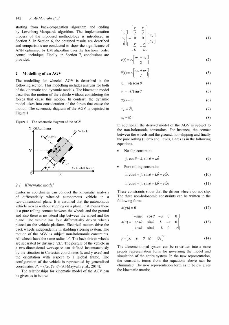
motion. The schematic diagram of the AGV is depicted in
Figure 1.
Figure 1 The schematic diagram of the AGV
2.1 Kinematic model
Cartesian coordinates can conduct the kinematic analysis
of differentially wheeled autonomous vehicle in a
two-dimensional plane. It is assumed that the autonomous
vehicle moves without slipping on a plane, that means there
is a pure rolling contact between the wheels and the ground
and also there is no lateral slip between the wheel and the
plane. The vehicle has four differentially driven wheels
placed on the vehicle platform. Electrical motors drive the
back wheels independently in skidding steering system. The
motion of the AGV is subject non-holonomic constraints.
All wheels have the same radius ‘r’. The back driven wheels
are separated by distance ‘2L’. The posture of the vehicle in
a two-dimensional workspace can defined instantaneously
by the situation in Cartesian coordinates (x and y-axes) and
the orientation with respect to a global frame. The
configuration of the vehicle is represented by generalised
coordinates, Pc = (Xc, Yc, θ) (Al-Mayyahi et al., 2014).
The relationships for kinematic model of the AGV can
be given as in below:
2 2
0 0
x
ry
l
r r
vω
vω
θ r r
L L
⎡ ⎤⎢ ⎥⎡ ⎤ ⎢ ⎥ ⎡ ⎤⎢ ⎥ = ⎢ ⎥ ⎢ ⎥⎢ ⎥ ⎣ ⎦⎢ ⎥⎢ ⎥⎣ ⎦ ⎢ − ⎥⎣ ⎦ (1)
( ) .2
r lω ωv t r
+⎡ ⎤= ⎢ ⎥⎣ ⎦ (2)
( ) .r lω ωθ t r
L
+⎡ ⎤= ⎢ ⎥⎣ ⎦ (3)
( ) coscx v t θ= (4)
( )sincy v t θ= (5)
( )θ t ω= (6)
r rω = ∅ (7)
l lω = ∅ (8)
In additional, the derived model of the AGV is subject to
the non-holonomic constraints. For instance, the contact
between the wheels and the ground, non-slipping and finally
the pure rolling (Fierro and Lewis, 1998) as in the following
equations.
• No slip constraint
cos sinc cy θ x θ aθ− = (9)
• Pure rolling constraint
cos sinc c rx θ y θ Lθ r+ + = ∅ (10)
cos sinc c lx θ y θ Lθ r+ − = ∅ (11)
These constraints show that the driven wheels do not slip.
The three non-holonomic constraints can be written in the
following form:
( ) 0A q q = (12)
sin cos 0 0
( ) cos sin 0
cos sin 0
θ θ a
A q θ θ L r
θ θ L r
− −⎡ ⎤⎢ ⎥= −⎢ ⎥⎢ ⎥− −⎣ ⎦ (13)
T
c c r lq x y θ⎡ ⎤= ∅ ∅⎣ ⎦ (14)
The aforementioned system can be re-written into a more
proper representation form for governing the model and
simulation of the entire system. In the new representation,
the constraint terms from the equations above can be
eliminated. The new representation form as in below gives
the kinematic matrix:

Levenberg-Marquardt optimised neural networks for trajectory tracking of autonomous ground vehicles 143
cos sin
cos
0 1
1
1
c
c
r
l
θ a θx Sinθ a
yV
q θ L ωr r
L
r r
−⎡ ⎤⎢ ⎥⎡ ⎤ ⎢ ⎥⎢ ⎥ ⎢ ⎥⎢ ⎥ ⎡ ⎤⎢ ⎥⎢ ⎥= = ⎢ ⎥⎢ ⎥⎢ ⎥ ⎣ ⎦∅ ⎢ ⎥⎢ ⎥ ⎢ ⎥⎢ ⎥∅⎣ ⎦ ⎢ ⎥−⎣ ⎦
(15)
where
vx the velocity of the vehicle in x-direction
vy the velocity of the vehicle in y-direction
θ moving vehicle orientation
ωr angular velocity of right wheel
ωl angular velocity of left wheel
ω angular velocity of vehicle.
This model is referred to a vehicle’s kinematic model since
it describes the velocities but not the forces or torques that
have effects on the velocity.
2.2 Dynamic model
The dynamic model of an autonomous vehicle represents
the study of the relationship between the various forces
action on a robot mechanism and their accelerations. This is
mainly used for simulation study and analysis of vehicle’s
design and a motion controller design for the vehicle. The
description of the mechanism of the robot movement is
given in terms of its component parts; bodies, joints and the
parameters that characterise them. In fact, several
parameters are required to define the dynamic model of a
given rigid body such inertia, centre of mass and applied
forces. The dynamic model of the AGV was derived based
on energy-Lagrangian method. The equation below is
described in a well-known formula (Fierro and Lewis,
1997).
( ) ( )( ) , ( )M q ω C q q ω F q B q T+ + = (16)
where
M(q) the symmetric positive definite inertia matrix
( , )C q q the centripetal and Coriolis matrix
( )F q the surface friction matrix
B(q) the input transformation matrix
T the input vector.
The equation (16) can be rewritten in a more appropriate
way as follows:
( )( ) , ( )M q ω C q q ω B q T+ + (17)
The above equation represents the dynamic behaviour of the
AGV. The final equation that governors the dynamic model
can be written in the simplified matrix form given below:
2
0 0
0 0
1 11
c
r
l
m ω ωmaθma I θ θmaθ
T
L L Tr
⎡ ⎤⎡ ⎤ ⎡ ⎤ − ⎡ ⎤+ ⎢ ⎥⎢ ⎥ ⎢ ⎥ ⎢ ⎥+⎣ ⎦ ⎣ ⎦ ⎣ ⎦⎣ ⎦⎡ ⎤ ⎡ ⎤= ⎢ ⎥ ⎢ ⎥−⎣ ⎦ ⎣ ⎦
(18)
The matrices elements are stated as follows:
2
0( )
0 c
mM q
ma I
⎡ ⎤= ⎢ ⎥+⎣ ⎦ (19)
( ) 0,
0
maθC q q
maθ⎡ ⎤−= ⎢ ⎥⎣ ⎦ (20)
1 11( )B q
L Lr
⎡ ⎤= ⎢ ⎥−⎣ ⎦ (21)
The relevant physical parameters of the AGV are shown in
Table 1.
Table 1 The physical parameters of the AGV
Parameter Description Value Unit
r Wheel radius 0.1 m
L The distance between the
one of driven wheel and the
axis of centre point
0.60 m
a The distance between the
centre of total mass and
centre axis of the back
driven wheels
0.25 m
m The mass of the vehicle
with driving wheels and DC
motors
20 kg
Ic The mass moment of inertia
about the centre of mass
4 Kgm2
d11 and d22 Surface friction coefficients 10 Each
2.3 Actuation system
Consider the driving control unit of the vehicle wheel, an
actuator is an electrical motor that drives a mechanical part
of a robotic mechanism. The actuator receives a control
signal directly from a control system to drive wheels into a
specified motion. A DC motor is used as an actuator in this
work. The model of DC motor is given in the following
equations:
m m aT k i= (22)
b b mv k ω= (23)
aa a a b
diE R i L v
dt= + + (24)
144 A. Al-Mayyahi et al.
mm m m L m
dωJ b ω T T
dt+ + = (25)
where
ωm = the angular speed of the motor
ia = the motor current
E = the applied voltage to the motor, which is Er for the
right motor and El for the left one
vb = the back e.m.f. voltage
Jm = the motor inertia
Tm = the motor torque
TL = load torque.
The physical parameters of the actuator are given in
Table 2.
Table 2 The physical parameters of the actuator
Parameter Description Value Unit
Ra The resistance of the
armature winding
8 Ω
La The inductance in the
motor winding
0 Henry
Jm The motor inertia 0 kgm2
km The torque constant 0.35 N.m/A
kb The back e.m.f. constant 0.35 V.s/rad
bm viscous friction 0 N.m.s
3 Fractional order systems
In this section, the generic control scheme will be explained.
It can be classified mainly into three parts. Firstly, the
fractional order PID controller is introduced as the first part
the concept of. Secondly, the fractional order PID
controller. In recent years, researchers reported that
factional order systems for modelling various systems more
adequately than conventional techniques. The fractional
order systems have main effect over the controller system
behaviour. For instance, to increase the speed of the
response, and decrease the steady-state error and relative
stability (Monje et al., 2010).
3.1 Fractional order calculus
Fractional calculus is a mathematical topic which studies
the ability of taking real number power of both the
differential and integration operators. There are several
definitions to describe the fractional derivative. The firmly
established definitions are Grunwald-Letnikov definition
and the Riemann-Liouville definition. The most frequently
used definition in fractional-order calculus is the
Riemann-Liouville definition, in which the fractional order
integration is defined as follows:
11
( ) ( ) ( )( )
t
tD f t t τ f τ dτ− −−Γ ∫β βα αβ (26)
where β represents the real order of the differential and
integral (0 < β < 1); α is the initial time instance, often
assumed to be zero; and t is the parameter for which both of
the differential and integral are taken. The Laplace and
Fourier transforms of the fractional derivative of f(t) is
given by:
[ ] 1
0
1
( ) ( ) ( )
nkk
t t t
k
L D f t S L f t S D f t− − ==⎡ ⎤ ⎡ ⎤= −⎣ ⎦ ⎣ ⎦∑β ββ (27)
For convenience, the second part on the right hand side of
equation (31) can be ignored when the derivatives of the
function f(t) are all equal to 0 at t = 0. Therefore, that
equation can be rewritten as in below:
( ) ( )tL D f t S F s⎡ ⎤ =⎣ ⎦β β (28)
where F(s) is the Laplace transformer of f(t).
3.2 Fractional order PID controller
The integral-differential equation defining the control action
of a fractional order PID controller is given by
( ) ( ) ( ) ( )p i du t K e t K D e t K D e t−= + + (29)
Applying Laplace transform to equation above with null
initial conditions, hence, the transfer function of the
controller can be expressed by:
( )i
f p d
KC s K K S
S= + + (30)
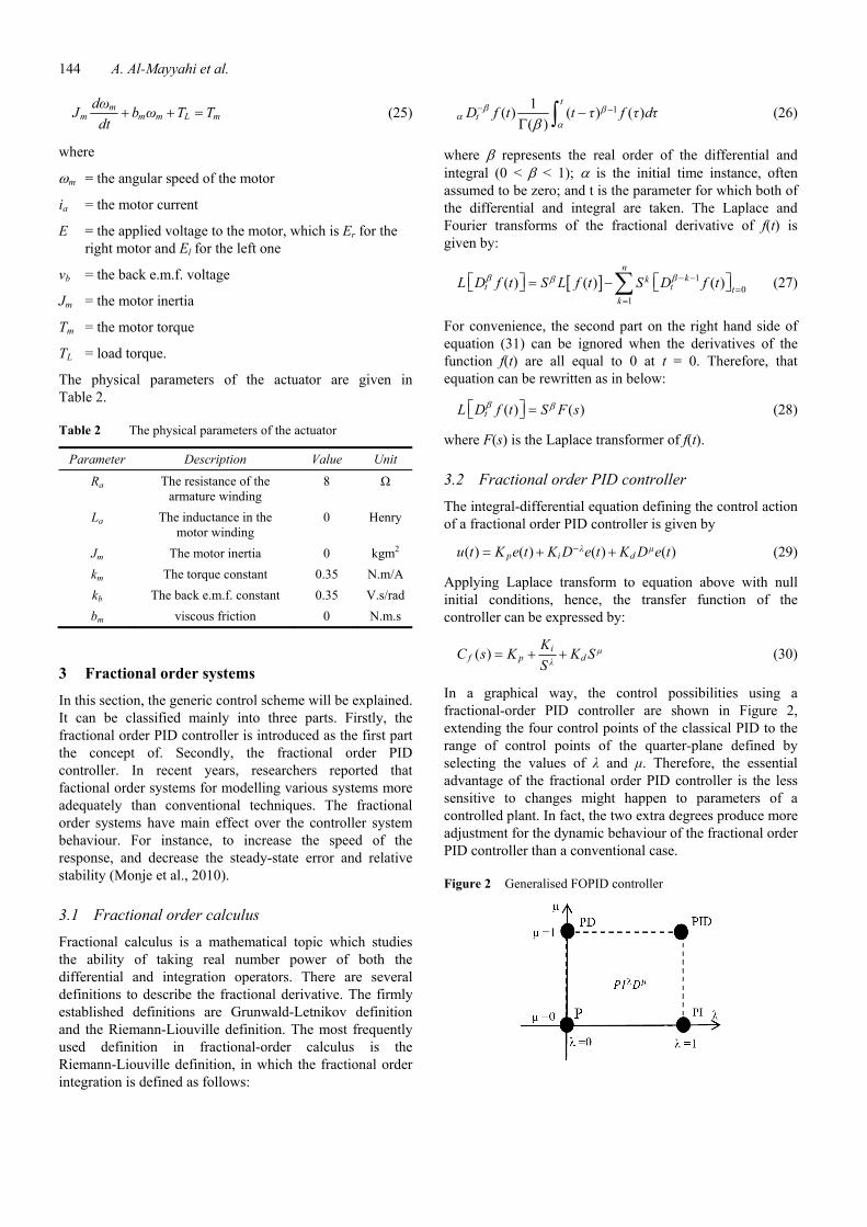
In a graphical way, the control possibilities using a
fractional-order PID controller are shown in Figure 2,
extending the four control points of the classical PID to the
range of control points of the quarter-plane defined by
selecting the values of and . Therefore, the essential
advantage of the fractional order PID controller is the less
sensitive to changes might happen to parameters of a
controlled plant. In fact, the two extra degrees produce more
adjustment for the dynamic behaviour of the fractional order
PID controller than a conventional case.
Figure 2 Generalised FOPID controller
Levenberg-Marquardt optimised neural networks for trajectory tracking of autonomous ground vehicles 145
4 Neural network architecture
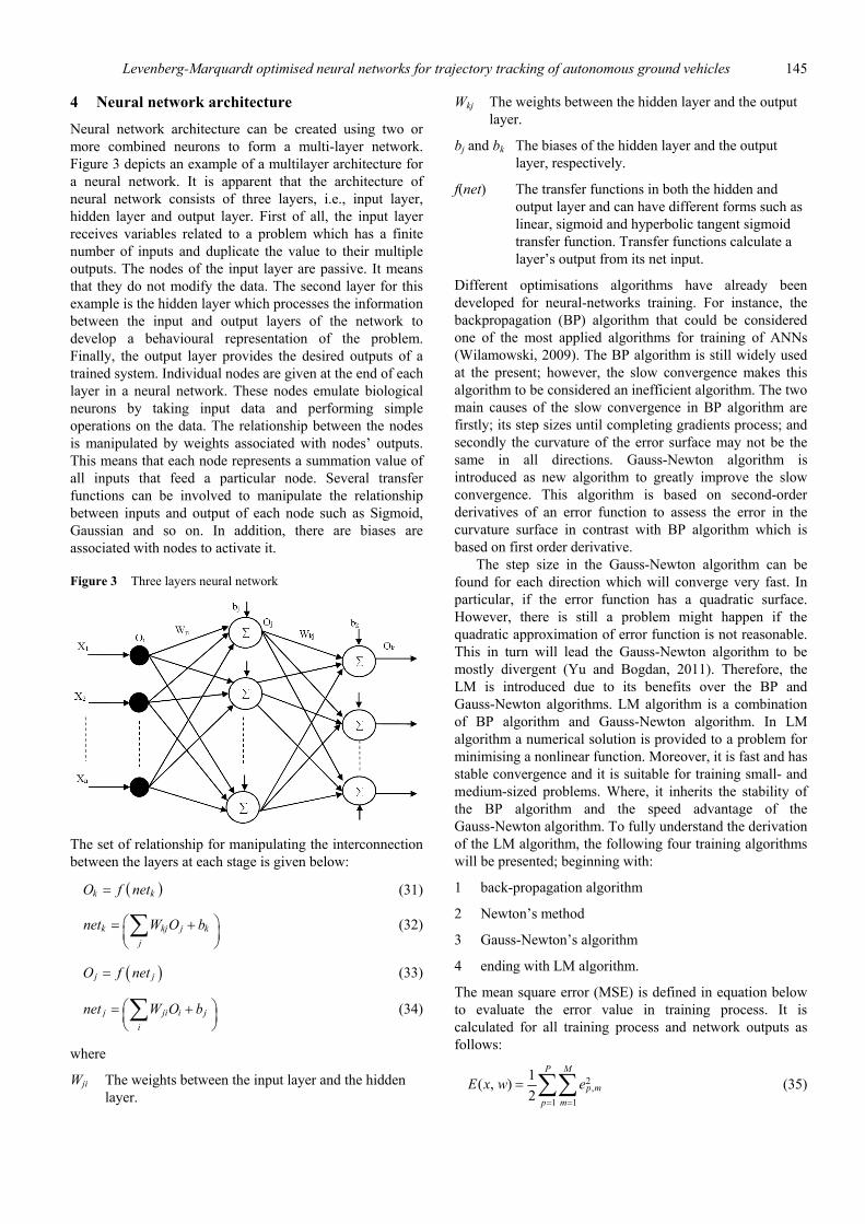
Neural network architecture can be created using two or
more combined neurons to form a multi-layer network.
Figure 3 depicts an example of a multilayer architecture for
a neural network. It is apparent that the architecture of
neural network consists of three layers, i.e., input layer,
hidden layer and output layer. First of all, the input layer
receives variables related to a problem which has a finite
number of inputs and duplicate the value to their multiple
outputs. The nodes of the input layer are passive. It means
that they do not modify the data. The second layer for this
example is the hidden layer which processes the information
between the input and output layers of the network to
develop a behavioural representation of the problem.
Finally, the output layer provides the desired outputs of a
trained system. Individual nodes are given at the end of each
layer in a neural network. These nodes emulate biological
neurons by taking input data and performing simple
operations on the data. The relationship between the nodes
is manipulated by weights associated with nodes’ outputs.
This means that each node represents a summation value of
all inputs that feed a particular node. Several transfer
functions can be involved to manipulate the relationship
between inputs and output of each node such as Sigmoid,
Gaussian and so on. In addition, there are biases are
associated with nodes to activate it.
Figure 3 Three layers neural network
The set of relationship for manipulating the interconnection
between the layers at each stage is given below:
( )k kO f net= (31)
k kj j k
j
net W O b⎛ ⎞= +⎜ ⎟⎝ ⎠∑ (32)
( )j jO f net= (33)
j ji i j
i
net W O b⎛ ⎞= +⎜ ⎟⎝ ⎠∑ (34)
where
Wji The weights between the input layer and the hidden
layer.
Wkj The weights between the hidden layer and the output
layer.
bj and bk The biases of the hidden layer and the output
layer, respectively.
f(net) The transfer functions in both the hidden and
output layer and can have different forms such as
linear, sigmoid and hyperbolic tangent sigmoid
transfer function. Transfer functions calculate a
layer’s output from its net input.
Different optimisations algorithms have already been
developed for neural-networks training. For instance, the
backpropagation (BP) algorithm that could be considered
one of the most applied algorithms for training of ANNs
(Wilamowski, 2009). The BP algorithm is still widely used
at the present; however, the slow convergence makes this
algorithm to be considered an inefficient algorithm. The two
main causes of the slow convergence in BP algorithm are
firstly; its step sizes until completing gradients process; and
secondly the curvature of the error surface may not be the
same in all directions. Gauss-Newton algorithm is
introduced as new algorithm to greatly improve the slow
convergence. This algorithm is based on second-order
derivatives of an error function to assess the error in the
curvature surface in contrast with BP algorithm which is
based on first order derivative.
The step size in the Gauss-Newton algorithm can be
found for each direction which will converge very fast. In
particular, if the error function has a quadratic surface.
However, there is still a problem might happen if the
quadratic approximation of error function is not reasonable.
This in turn will lead the Gauss-Newton algorithm to be
mostly divergent (Yu and Bogdan, 2011). Therefore, the
LM is introduced due to its benefits over the BP and
Gauss-Newton algorithms. LM algorithm is a combination
of BP algorithm and Gauss-Newton algorithm. In LM
algorithm a numerical solution is provided to a problem for
minimising a nonlinear function. Moreover, it is fast and has
stable convergence and it is suitable for training small- and
medium-sized problems. Where, it inherits the stability of
the BP algorithm and the speed advantage of the
Gauss-Newton algorithm. To fully understand the derivation
of the LM algorithm, the following four training algorithms
will be presented; beginning with:
1 back-propagation algorithm
2 Newton’s method
3 Gauss-Newton’s algorithm
4 ending with LM algorithm.
The mean square error (MSE) is defined in equation below
to evaluate the error value in training process. It is
calculated for all training process and network outputs as
follows:
2,
1 1
1( , )
2
P M
p m
p m
E x w e
= == ∑∑ (35)
146 A. Al-Mayyahi et al.
, , ,p m p m p me d O= − (36)
where
x the network input
w the weight of network
p the number of patterns
m the number of outputs
ep,m the training error
d the required output
o the actual output
4.1 Back-propagation algorithm
The BP algorithm uses for finding the minimum of the error
function. It utilises a gradient descent method to calculate
the error in weight space to be a solution of the learning
problem. Therefore, the error function can be minimised by
using iterative process of gradient descent as shown in
equation below. The index g is defined as the first-order
derivative of total error function.
1 2
( , )T
N
E x w E E Eg
w w w w
∂ ∂ ∂ ∂⎡ ⎤= = ⎢ ⎥∂ ∂ ∂ ∂⎣ ⎦ (37)
The update rule for each weight of the BP algorithm could
be written as follows:
1k k kw w g+ = −α (38)
where
α the learning rate or it is called the step size
N the number of weights
i and j the indices of weights, from 1 to N
k iterations number.
4.2 Newton’s algorithm
In Newton’s method, it is assumed that all the gradient
components, i.e., g1, g2, …, gN are functions of weights
where all weights are linearly independent:
( )( )( )
1 1 1 2
2 1 2 2
1 2
, , ...,
, , ...,
, , ...,
N
N
N N N
g F w w w
g F w w w
g F w w w
⎧ =⎪ =⎪⎨⎪⎪ =⎩ (39)
where F1, F2, …, FN represent nonlinear relationships
between gradient components and weights. Thus, to unfold
each gi (i = 1, 2, …, N) in equations (39) by Taylor series
and take the first-order approximation we can get:
1 1 11 1,0 1 2
1 2
2 2 22 2,0 1 2
1 2
,0 1 2
1 2
N
N
N
N
N N NN N N
N
g g gg g w w w
w w w
g g gg g w w w
w w w
g g gg g w w w
w w w
∂ ∂ ∂⎧ ≈ + Δ + Δ + + Δ⎪ ∂ ∂ ∂⎪ ∂ ∂ ∂⎪ ≈ + Δ + Δ + + Δ⎪ ∂ ∂ ∂⎨⎪⎪ ∂ ∂ ∂⎪ ≈ + Δ + Δ + + Δ⎪ ∂ ∂ ∂⎩
(40)
From the definition of gradient descent g in equation (37), it
could be determined that
2i i
j j i j
E
g Ew
w w w w
∂⎛ ⎞∂ ⎜ ⎟∂ ∂∂⎝ ⎠= =∂ ∂ ∂ ∂ (41)
By substituting equation (41) into (40), we get;
2 2 2
1 1,0 1 22
1 2 11
2 2 2
2 2,0 1 22
2 1 22
2 2 2
,0 1 22
1 2
N
N
N
N
N N N
N N N
E E Eg g w w w
w w w w w
E E Eg g w w w
w w w w w
E E Eg g w w w
w w w w w
∂ ∂ ∂⎧ ≈ + Δ + Δ + + Δ⎪ ∂ ∂ ∂ ∂ ∂⎪⎪ ∂ ∂ ∂≈ + Δ + Δ + + Δ⎪ ∂ ∂ ∂ ∂ ∂⎨⎪⎪⎪ ∂ ∂ ∂≈ + Δ + Δ + + Δ⎪ ∂ ∂ ∂ ∂ ∂⎩
(42)
In order to obtain the minima of error function, gradient
descent should be zero of each component. Therefore, the
left sides of the equation (42) are all set to zero, hence,
2 2 2
1,0 1 22
1 2 11
2 2 2
2,0 1 22
2 1 22
2 2 2
,0 1 22
1 2
0
0
0
N
N
N
N
N N
N N N
E E Eg w w w
w w w w w
E E Eg w w w
w w w w w
E E Eg w w w
w w w w w
∂ ∂ ∂⎧ ≈ + Δ = Δ + + Δ⎪ ∂ ∂ ∂ ∂ ∂⎪⎪ ∂ ∂ ∂≈ + Δ = Δ + + Δ⎪ ∂ ∂ ∂ ∂ ∂⎨⎪⎪⎪ ∂ ∂ ∂≈ + Δ = Δ + + Δ⎪ ∂ ∂ ∂ ∂ ∂⎩
(43)
By combining equation (37) with (43), we obtain;
2 2
1,0 1 22
1 1 21
2
1
2 2
2,0 1 22
2 2 1 2
2
2
2 2
,0 1 2
1 2
2
2
N
N
N
N
N
N N N
N
N
E E Eg w w
w w w w
ew
w w
E E Eg w w
w w w w
ew
w w
E E Eg w w
w w w w w
ew
w
∂ ∂ ∂⎧ − = − ≈ + Δ + Δ⎪ ∂ ∂ ∂ ∂⎪⎪ ∂+ + Δ⎪ ∂ ∂⎪⎪ ∂ ∂ ∂− = − ≈ + Δ + Δ⎪ ∂ ∂ ∂ ∂⎪⎪ ∂⎨ + + Δ⎪ ∂ ∂⎪⎪⎪ ∂ ∂ ∂⎪− = − ≈ + Δ + Δ⎪ ∂ ∂ ∂ ∂ ∂⎪ ∂⎪ + + Δ⎪ ∂⎩
(44)

Levenberg-Marquardt optimised neural networks for trajectory tracking of autonomous ground vehicles 147
From the equation above, it is obvious that there are N
parameters for N equations. This means all Δwi can be
calculated during the learning process, the weights will be
updated iteratively. Equation (44) can be written in a matrix
form as in follows:
11
2
2
2 2 2
21 2 11
12 2 2
222 1 22
2 2 2
21 2
N
N
N
N
N
N N N
E
wg
Eg
w
gE
w
E E E
w w w w ww
E E Ew
w w w w w
wE E E
w w w w w
∂⎡ ⎤−⎢ ⎥∂⎢ ⎥−⎡ ⎤ ∂⎢ ⎥⎢ ⎥ −− ⎢ ⎥⎢ ⎥ = ∂⎢ ⎥⎢ ⎥ ⎢ ⎥⎢ ⎥− ⎢ ⎥⎣ ⎦ ∂⎢ ⎥−⎢ ⎥∂⎣ ⎦∂ ∂ ∂⎡ ⎤⎢ ⎥∂ ∂ ∂ ∂ ∂⎢ ⎥ Δ⎡ ⎤⎢ ⎥∂ ∂ ∂ ⎢ ⎥Δ⎢ ⎥ ⎢ ⎥= ×∂ ∂ ∂ ∂ ∂⎢ ⎥ ⎢ ⎥⎢ ⎥ ⎢ ⎥⎢ ⎥ Δ⎣ ⎦∂ ∂ ∂⎢ ⎥⎢ ⎥∂ ∂ ∂ ∂ ∂⎣ ⎦
(45)
where the square matrix is Hessian matrix:
2 2 2
21 2 11
2 2 2
22 1 22
2 2 2
21 2
N
N
N N N
E E E
w w w w w
E E E
H w w w w w
E E E
w w w w w
∂ ∂ ∂⎡ ⎤⎢ ⎥∂ ∂ ∂ ∂ ∂⎢ ⎥⎢ ⎥∂ ∂ ∂⎢ ⎥= ∂ ∂ ∂ ∂ ∂⎢ ⎥⎢ ⎥⎢ ⎥∂ ∂ ∂⎢ ⎥⎢ ⎥∂ ∂ ∂ ∂ ∂⎣ ⎦
(46)
By combining equations (37) and (45) with equation (46)
g H w− = Δ (47)
Thus,
1w H g−Δ = − (48)
Therefore, in Newton’s method, the incremental updating
rule for weights is given below:
11k k kkw w H g−+ = − (49)
H is defined as a Hessian matrix that provides the
second-order derivatives of total error function and gives
the proper evaluation on the change of gradient descent.
4.3 Gauss-Newton algorithm
In Gauss-Newton algorithm, Jacobian matrix J is introduced
to simplify the calculation process due to the complexity
inherited the second-order derivatives of total error function
with Newton’s method.
1,1 1,1 1,1
1 2
1,2 1,2 1,2
1 2
1, 1, 1,
1 2
,1 ,1 ,1
1 2
,2 ,2 ,2
1 2
, , ,
1 2
N
N
M M M
N
p p p
N
p p p
N
p m p m p m
N
e e e
w w w
e e e
w w w
e e e
w w w
J
e e e
w w w
e e e
w w w
e e e
w w w
∂ ∂ ∂⎡ ⎤⎢ ⎥∂ ∂ ∂⎢ ⎥∂ ∂ ∂⎢ ⎥⎢ ⎥∂ ∂ ∂⎢ ⎥⎢ ⎥⎢ ⎥∂ ∂ ∂⎢ ⎥⎢ ⎥∂ ∂ ∂⎢ ⎥= ⎢ ⎥⎢ ∂ ∂ ∂⎢ ∂ ∂ ∂⎢⎢ ∂ ∂ ∂⎢ ∂ ∂ ∂⎢⎢⎢∂ ∂ ∂⎢⎢ ∂ ∂ ∂⎣ ⎦
⎥⎥⎥⎥⎥⎥⎥⎥⎥⎥
(50)
By integrating equations (35) and (37), gradient descent’s
elements can be calculated as follows:
2,
1 1
,,
1 1
1
2
p m
p mp m
i
i i
p mp m
p m
ip m
eE
gw w
ee
w
= =
= =
⎛ ⎞∂ ⎜ ⎟∂ ⎝ ⎠= =∂ ∂∂⎛ ⎞= ⎜ ⎟∂⎝ ⎠
∑ ∑∑∑
(51)
Combining equations (50) and (51), the relationship
between gradient descent (g) and Jacobian matrix (J) and
would be
g Je= (52)
where the error (e) has the following form;
1,1
1,2
1,
,1
,2
,
m
p
p
p m
e
e
e
e
e
e
e
⎡ ⎤⎢ ⎥⎢ ⎥⎢ ⎥⎢ ⎥⎢ ⎥⎢ ⎥= ⎢ ⎥⎢ ⎥⎢ ⎥⎢ ⎥⎢ ⎥⎢ ⎥⎣ ⎦
(53)
Inserting equation (35) into (36), the elements of Hessian
matrix, i.e., ith row and jth column can be calculated as
2 2,2 1 1
,
, ,,
1 1
1
2
p m
p mp m
i j
i j i j
p mp m p m
i j
i jp m
eE
hw w w w
e eS
w w
= =
= =
⎛ ⎞∂ ⎜ ⎟∂ ⎝ ⎠= =∂ ∂ ∂ ∂∂ ∂= +∂ ∂
∑ ∑∑∑
(54)
where Si,j is equal to

148 A. Al-Mayyahi et al.
2,
, ,
1 1
p mp m
i j p m
i jp m
eS e
w w= =∂= ∂ ∂∑∑ (55)
From Newton’s method, it is assumed that the Si,j is closed
to zero. Therefore, the relationship between Jacobian matrix
(J) and Hessian matrix (H) can be rewritten as follow:
TH J J≈ (56)
By combining equations (49), (52) and (56), the weights
updating rule of the Gauss-Newton algorithm can be given
as in below:
( ) 1
1T
k k k k kkw w J J J e−+ = − (57)
4.4 LM algorithm
This algorithm is an approximation to Newton’s method
(Hagan and Menhaj, 1994). In order to make sure that the
approximated Hessian matrix is invertible, LM algorithm
introduces another approximation to Hessian matrix as
follows:
TH J J I≈ + (58)
where
combination coefficient and it is always positive,
I the identity matrix.
By combining equations (57) and (58), the update rule
for weights of LM algorithm can be obtained as follows:
( ) 1
1T
k k k k kkw w J J I J e−+ = − + (59)
The LM algorithm switches between the two BP algorithms
and the Gauss-Newton algorithm during the training
process. Two situations will be considered in LM algorithm.
Firstly, if the combination coefficient ( ) is very small,
hence, equation (59) is approaching to equation (57) and
Gauss-Newton algorithm is used. However, if combination
coefficient ( ) is very large, equation (59) approximates to
equation (38) and the BP algorithm is used.
The following steps describe the training process of LM
algorithms:
Step 1 Generate the initial weights.
Step 2 update weights using equation (59).
Step 3 Evaluate the error at each updated weights.
Step 4 If the new error is increased after updating, go to
Step 2 and try an update again after increasing
combination coefficient by a suitable factor.
Otherwise, go to Step 5.
Step 5 If the new error is decreased, then, compare the
new error with the required value. If the new error
is smaller than the required value, then, stop
learning. Otherwise, go to Step 2.
Table 3 summarises the update rules for various algorithms.
5 Trajectory tracking control scheme of AGV
The implementation process of the entire control scheme of
the ANN and the AGV model can be classified into three
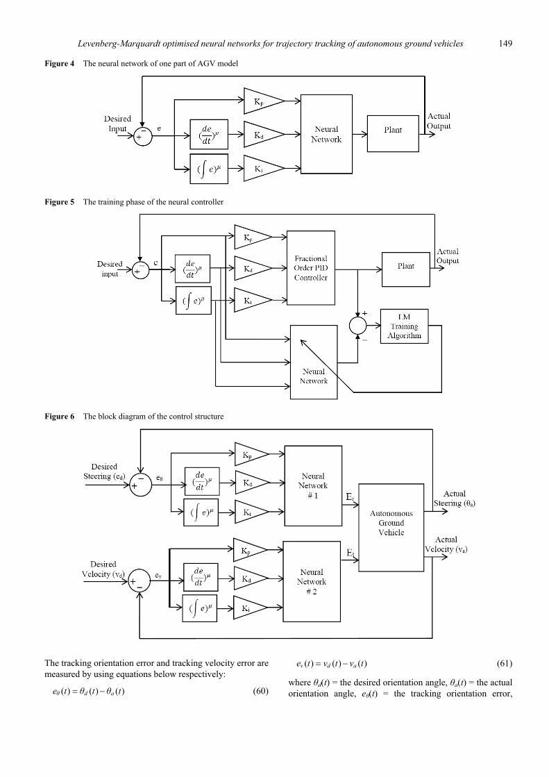
parts. The first one is depicted in Figure 4 that represents
the relationship between a FOPID-NN controller and a
plant. The second part is represented by Figure 5 which
shows the training phase for a model. The optimal values of
the trainable parameters of the neural controller are met
using MSE cost function. The entire control scheme is
depicted in Figure 6. Two trained neural network controllers
are used for driving the right and left motor voltage of the
vehicle separately to enable the AGV of tracking a
predefined trajectory. The first controller receives the error
between the desired generated trajectory and actual
trajectory in order to control the ordination angle of the
AGV. Therefore, the vehicle must change its orientation as
needed to track the desired trajectory. The output of this
controller is directly connected to the right motor voltage.
The second controller utilises the error signal between the
desired and actual velocity as an input. The desired velocity
is assumed to a constant during the tracking process. The
output of this controller is fed to the left motor voltage of
the AGV. The main purpose of the second controller is to
maintain a constant velocity for controlling the motion. The
input and output data obtained from the FOPID controller
that implemented in an earlier work are used to train the
parameters of neural controller using the LM training
algorithm.
Table 3 Specifications of various algorithms
Algorithms Update rules Convergence Computation complexity
BP algorithm wk+1 = wk – αgk Stable, slow Gradient
Newton algorithm 11k k kkw w H g−+ = − Unstable, fast Gradient and Hessian
Gauss-Newton algorithm ( ) 1
1T
k k k k kkw w J J J e−
+ = − Unstable, fast Jacobian
Levenberg-Marquardt slgorithm ( ) 1
1T
k k k k kkw w J J I J e−
+ = − + stable, fast Jacobian
Levenberg-Marquardt optimised neural networks for trajectory tracking of autonomous ground vehicles 149
Figure 4 The neural network of one part of AGV model
Figure 5 The training phase of the neural controller
Figure 6 The block diagram of the control structure
The tracking orientation error and tracking velocity error are
measured by using equations below respectively:
( ) ( ) ( )θ d ae t θ t θ t= − (60)
( ) ( ) ( )v d ae t v t v t= − (61)
where θd(t) = the desired orientation angle, θa(t) = the actual
orientation angle, eθ(t) = the tracking orientation error,
150 A. Al-Mayyahi et al.
vr(t) = the desired velocity, va(t) = the actual velocity, and
ev(t) = tracking velocity error.
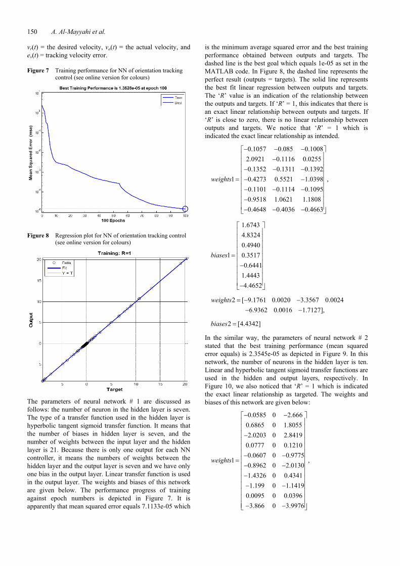
Figure 7 Training performance for NN of orientation tracking
control (see online version for colours)
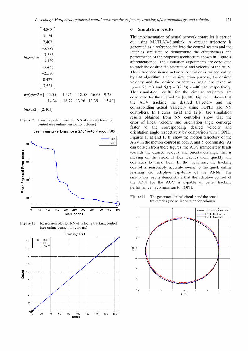
Figure 8 Regression plot for NN of orientation tracking control
(see online version for colours)
The parameters of neural network # 1 are discussed as
follows: the number of neuron in the hidden layer is seven.
The type of a transfer function used in the hidden layer is
hyperbolic tangent sigmoid transfer function. It means that
the number of biases in hidden layer is seven, and the
number of weights between the input layer and the hidden
layer is 21. Because there is only one output for each NN
controller, it means the numbers of weights between the
hidden layer and the output layer is seven and we have only
one bias in the output layer. Linear transfer function is used
in the output layer. The weights and biases of this network
are given below. The performance progress of training
against epoch numbers is depicted in Figure 7. It is
apparently that mean squared error equals 7.1133e-05 which
is the minimum average squared error and the best training
performance obtained between outputs and targets. The
dashed line is the best goal which equals 1e-05 as set in the
MATLAB code. In Figure 8, the dashed line represents the
perfect result (outputs = targets). The solid line represents
the best fit linear regression between outputs and targets.
The ‘R’ value is an indication of the relationship between
the outputs and targets. If ‘R’ = 1, this indicates that there is
an exact linear relationship between outputs and targets. If
‘R’ is close to zero, there is no linear relationship between
outputs and targets. We notice that ‘R’ = 1 which is
indicated the exact linear relationship as intended.
0.1057 0.085 0.1008
2.0921 0.1116 0.0255
0.1352 0.1311 0.1392
1 ,0.4273 0.5521 1.0398
0.1101 0.1114 0.1095
0.9518 1.0621 1.1808
0.4648 0.4036 0.4663
weights
− − −⎡ ⎤⎢ ⎥−⎢ ⎥⎢ ⎥− − −⎢ ⎥= − −⎢ ⎥⎢ ⎥− − −⎢ ⎥−⎢ ⎥⎢ ⎥− − −⎣ ⎦
1.6743
4.8324
0.4940
1 0.3517
0.6441
1.4443
4.4652
biases
⎡ ⎤⎢ ⎥⎢ ⎥⎢ ⎥⎢ ⎥= ⎢ ⎥⎢ ⎥−⎢ ⎥⎢ ⎥⎢ ⎥−⎣ ⎦
2 [ 9.1761 0.0020 3.3567 0.0024
6.9362 0.0016 1.7127],
weights = − −− −
2 [4.4342]biases =
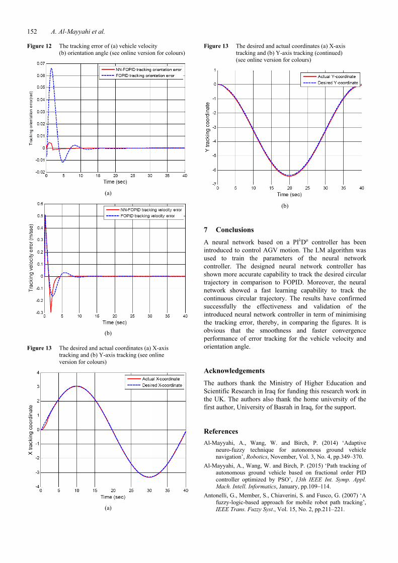
In the similar way, the parameters of neural network # 2
stated that the best training performance (mean squared
error equals) is 2.3545e-05 as depicted in Figure 9. In this
network, the number of neurons in the hidden layer is ten.
Linear and hyperbolic tangent sigmoid transfer functions are
used in the hidden and output layers, respectively. In
Figure 10, we also noticed that ‘R’ = 1 which is indicated
the exact linear relationship as targeted. The weights and
biases of this network are given below:
0.0585 0 2.666
0.6865 0 1.8055
2.0203 0 2.8419
0.0777 0 0.1210
0.0607 0 0.97751 ,
0.8962 0 2.0130
1.4326 0 0.4341
1.199 0 1.1419
0.0095 0 0.0396
3.866 0 3.9976
weights
− −⎡ ⎤⎢ ⎥⎢ ⎥⎢ ⎥−⎢ ⎥⎢ ⎥⎢ ⎥− −⎢ ⎥= − −⎢ ⎥⎢ ⎥−⎢ ⎥− −⎢ ⎥⎢ ⎥⎢ ⎥⎢ ⎥− −⎣ ⎦
Levenberg-Marquardt optimised neural networks for trajectory tracking of autonomous ground vehicles 151
4.808
3.134
7.407
5.789
3.5651
3.179
3.458
2.550
0.427
7.531
biases
⎡ ⎤⎢ ⎥⎢ ⎥⎢ ⎥⎢ ⎥−⎢ ⎥⎢ ⎥−⎢ ⎥= −⎢ ⎥⎢ ⎥−⎢ ⎥−⎢ ⎥⎢ ⎥⎢ ⎥⎢ ⎥⎣ ⎦
2 [ 15.55 1.676 18.58 36.65 9.25
14.34 16.79 13.26 13.39 15.40]
weights = − − −− − − −
2 [2.405]biases =
Figure 9 Training performance for NN of velocity tracking
control (see online version for colours)
Figure 10 Regression plot for NN of velocity tracking control
(see online version for colours)
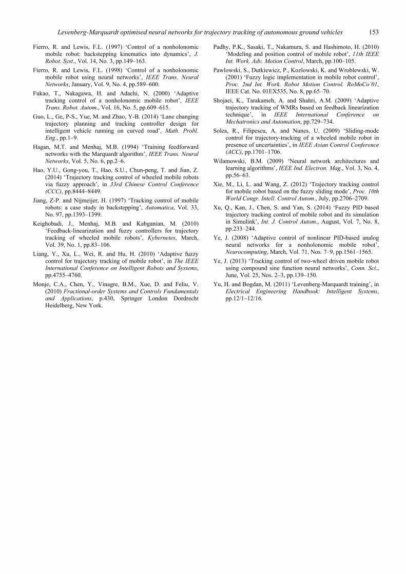
6 Simulation results
The implementation of neural network controller is carried
out using MATLAB-Simulink. A circular trajectory is
generated as a reference fed into the control system and the
latter is simulated to demonstrate the effectiveness and
performance of the proposed architecture shown in Figure 4
aforementioned. The simulation experiments are conducted
to track the desired the orientation and velocity of the AGV.
The introduced neural network controller is trained online
by LM algorithm. For the simulation purpose, the desired
velocity and the desired orientation angle are taken as
vd = 0.25 m/s and θd(t) = [(2π*t) / –40] rad, respectively.
The simulation results for the circular trajectory are
conducted for the interval t ∈ [0, 40]. Figure 11 shows that
the AGV tracking the desired trajectory and the
corresponding actual trajectory using FOPID and NN
controllers. In Figures 12(a) and 12(b), the simulation
results obtained from NN controller show that the
error of linear velocity and orientation angle converge
faster to the corresponding desired velocity and
orientation angle respectively by comparison with FOPID.
Figures 13(a) and 13(b) show the motion trajectory of the
AGV in the motion control in both X and Y coordinates. As
can be seen from these figures, the AGV immediately heads
towards the desired velocity and orientation angle that is
moving on the circle. It then reaches them quickly and
continues to track them. In the meantime, the tracking
control is reasonably accurate owing to the quick online
learning and adaptive capability of the ANNs. The
simulation results demonstrate that the adaptive control of
the ANN for the AGV is capable of better tracking
performance in comparison to FOPID.
Figure 11 The generated desired circular and the actual
trajectories (see online version for colours)
152 A. Al-Mayyahi et al.
Figure 12 The tracking error of (a) vehicle velocity
(b) orientation angle (see online version for colours)
(a)
(b)
Figure 13 The desired and actual coordinates (a) X-axis
tracking and (b) Y-axis tracking (see online
version for colours)
(a)
Figure 13 The desired and actual coordinates (a) X-axis
tracking and (b) Y-axis tracking (continued)
(see online version for colours)
(b)
7 Conclusions
A neural network based on a PI D controller has been
introduced to control AGV motion. The LM algorithm was
used to train the parameters of the neural network
controller. The designed neural network controller has
shown more accurate capability to track the desired circular
trajectory in comparison to FOPID. Moreover, the neural
network showed a fast learning capability to track the
continuous circular trajectory. The results have confirmed
successfully the effectiveness and validation of the
introduced neural network controller in term of minimising
the tracking error, thereby, in comparing the figures. It is
obvious that the smoothness and faster convergence
performance of error tracking for the vehicle velocity and
orientation angle.
Acknowledgements
The authors thank the Ministry of Higher Education and
Scientific Research in Iraq for funding this research work in
the UK. The authors also thank the home university of the
first author, University of Basrah in Iraq, for the support.
References
Al-Mayyahi, A., Wang, W. and Birch, P. (2014) ‘Adaptive
neuro-fuzzy technique for autonomous ground vehicle
navigation’, Robotics, November, Vol. 3, No. 4, pp.349–370.
Al-Mayyahi, A., Wang, W. and Birch, P. (2015) ‘Path tracking of
autonomous ground vehicle based on fractional order PID
controller optimized by PSO’, 13th IEEE Int. Symp. Appl.
Mach. Intell. Informatics, January, pp.109–114.
Antonelli, G., Member, S., Chiaverini, S. and Fusco, G. (2007) ‘A
fuzzy-logic-based approach for mobile robot path tracking’,
IEEE Trans. Fuzzy Syst., Vol. 15, No. 2, pp.211–221.
Levenberg-Marquardt optimised neural networks for trajectory tracking of autonomous ground vehicles 153
Fierro, R. and Lewis, F.L. (1997) ‘Control of a nonholonomic
mobile robot: backstepping kinematics into dynamics’, J.
Robot. Syst., Vol. 14, No. 3, pp.149–163.
Fierro, R. and Lewis, F.L. (1998) ‘Control of a nonholonomic
mobile robot using neural networks’, IEEE Trans. Neural
Networks, January, Vol. 9, No. 4, pp.589–600.
Fukao, T., Nakagawa, H. and Adachi, N. (2000) ‘Adaptive
tracking control of a nonholonomic mobile robot’, IEEE
Trans. Robot. Autom., Vol. 16, No. 5, pp.609–615.
Guo, L., Ge, P-S., Yue, M. and Zhao, Y-B. (2014) ‘Lane changing
trajectory planning and tracking controller design for
intelligent vehicle running on curved road’, Math. Probl.
Eng., pp.1–9.
Hagan, M.T. and Menhaj, M.B. (1994) ‘Training feedforward
networks with the Marquardt algorithm’, IEEE Trans. Neural
Networks, Vol. 5, No. 6, pp.2–6.
Hao, Y.U., Gong-you, T., Hao, S.U., Chun-peng, T. and Jian, Z.
(2014) ‘Trajectory tracking control of wheeled mobile robots
via fuzzy approach’, in 33rd Chinese Control Conference
(CCC), pp.8444–8449.
Jiang, Z-P. and Nijmeijer, H. (1997) ‘Tracking control of mobile
robots: a case study in backstepping’, Automatica, Vol. 33,
No. 97, pp.1393–1399.
Keighobadi, J., Menhaj, M.B. and Kabganian, M. (2010)
‘Feedback-linearization and fuzzy controllers for trajectory
tracking of wheeled mobile robots’, Kybernetes, March,
Vol. 39, No. 1, pp.83–106.
Liang, Y., Xu, L., Wei, R. and Hu, H. (2010) ‘Adaptive fuzzy
control for trajectory tracking of mobile robot’, in The IEEE
International Conference on Intelligent Robots and Systems,
pp.4755–4760.
Monje, C.A., Chen, Y., Vinagre, B.M., Xue, D. and Feliu, V.
(2010) Fractional-order Systems and Controls Fundamentals
and Applications, p.430, Springer London Dordrecht
Heidelberg, New York.
Padhy, P.K., Sasaki, T., Nakamura, S. and Hashimoto, H. (2010)
‘Modeling and position control of mobile robot’, 11th IEEE
Int. Work. Adv. Motion Control, March, pp.100–105.
Pawlowski, S., Dutkiewicz, P., Kozlowski, K. and Wroblewski, W.
(2001) ‘Fuzzy logic implementation in mobile robot control’,
Proc. 2nd Int. Work. Robot Motion Control. RoMoCo’01,
IEEE Cat. No. 01EX535, No. 8, pp.65–70.
Shojaei, K., Tarakameh, A. and Shahri, A.M. (2009) ‘Adaptive
trajectory tracking of WMRs based on feedback linearization
technique’, in IEEE International Conference on
Mechatronics and Automation, pp.729–734.
Solea, R., Filipescu, A. and Nunes, U. (2009) ‘Sliding-mode
control for trajectory-tracking of a wheeled mobile robot in
presence of uncertainties’, in IEEE Asian Control Conference
(ACC), pp.1701–1706.
Wilamowski, B.M. (2009) ‘Neural network architectures and
learning algorithms’, IEEE Ind. Electron. Mag., Vol. 3, No. 4,
pp.56–63.
Xie, M., Li, L. and Wang, Z. (2012) ‘Trajectory tracking control
for mobile robot based on the fuzzy sliding mode’, Proc. 10th
World Congr. Intell. Control Autom., July, pp.2706–2709.
Xu, Q., Kan, J., Chen, S. and Yan, S. (2014) ‘Fuzzy PID based
trajectory tracking control of mobile robot and its simulation
in Simulink’, Int. J. Control Autom., August, Vol. 7, No. 8,
pp.233–244.
Ye, J. (2008) ‘Adaptive control of nonlinear PID-based analog
neural networks for a nonholonomic mobile robot’,
Neurocomputing, March, Vol. 71, Nos. 7–9, pp.1561–1565.
Ye, J. (2013) ‘Tracking control of two-wheel driven mobile robot
using compound sine function neural networks’, Conn. Sci.,
June, Vol. 25, Nos. 2–3, pp.139–150.
Yu, H. and Bogdan, M. (2011) ‘Levenberg-Marquardt training’, in
Electrical Engineering Handbook: Intelligent Systems,
pp.12/1–12/16.