leverage causes fat tails and clustered volatility · pdf fileleverage causes fat tails and...

Quantitative Finance, Vol. 12, No. 5, May 2012, 695–707

Leverage causes fat tails and clustered volatility

STEFAN THURNER*yzx, J. DOYNE FARMERz and JOHN GEANAKOPLOSz{k

ySection of Science of Complex Systems, Medical University of Vienna, Spitalgasse 23, Vienna A-1090, AustriazSanta Fe Institute, 1399 Hyde Park Road, Santa Fe, NM 87501, USA

xIIASA, Schlossplatz 1, A-2361 Laxenburg, Austria{James Tobin Professor of Economics, Yale University, New Haven, CT, USA

kEllington Capital Management, Old Greenwich, CT, USA

(Received 31 January 2011; in final form 29 February 2012)

We build a simple model of leveraged asset purchases with margin calls. Investment funds usewhat is perhaps the most basic financial strategy, called ‘value investing’, i.e. systematicallyattempting to buy underpriced assets. When funds do not borrow, the price fluctuations of theasset are approximately normally distributed and uncorrelated across time. This changes whenthe funds are allowed to leverage, i.e. borrow from a bank, which allows them to purchasemore assets than their wealth would otherwise permit. During good times, funds that use moreleverage have higher profits, increasing their wealth and making them dominant in the market.However, if a downward price fluctuation occurs while one or more funds is fully leveraged,the resulting margin call causes them to sell into an already falling market, amplifying thedownward price movement. If the funds hold large positions in the asset, this can causesubstantial losses. This in turn leads to clustered volatility: before a crash, when the valuefunds are dominant, they damp volatility, and after the crash, when they suffer severe losses,volatility is high. This leads to power-law tails, which are both due to the leverage-inducedcrashes and due to the clustered volatility induced by the wealth dynamics. This is in contrastto previous explanations of fat tails and clustered volatility, which depended on ‘irrationalbehavior’, such as trend following. A standard (supposedly more sophisticated) risk controlpolicy in which individual banks base leverage limits on volatility causes leverage to riseduring periods of low volatility, and to contract more quickly when volatility becomes high,making these extreme fluctuations even worse.

Keywords: Systemic risk; Clustered volatility; Fat tails; Crash; Margin calls; Leverage

JEL Classification: E32, E37, G01, G12, G14

1. Introduction

Recent events in financial markets have underscored thedangerous consequences of the use of excessive credit. Atthe most basic level the problem is obvious: if a firm buysassets with borrowed money, then under extreme marketconditions it may owe more money than it has anddefaults. If this happens on a sufficiently wide scale, then itcan severely stress creditors and cause them to fail as well.

We show here that a special but extremely widespreadkind of credit called collateralized loans with margin callshas a more pervasive effect: when used excessively it cancause default and crashes, but it also leaves a signature

even when there is no default or crash. These kinds ofloans have already been identified as a major culprit in therecent crisis, and in previous near crises as well.> But weshow here that they create a dynamic in asset pricefluctuations that manifests itself at all time scales and toall degrees. The extraordinary crisis of the last couple ofyears is just one extreme (but not extremal) point on acontinuum.

By taking out a collateralized loan a buyer of stocks ormortgage-backed securities can put together a portfoliothat is worth a multiple of the cash he has available fortheir purchase. In 2006 this multiple or ‘leverage’ reached60 to 1 for AAA-rated mortgage securities, and 16 to 1 for

*Corresponding author. Email: [email protected]>For previous equilibrium-based analyses of leverage that show that prices crash before default actually occurs, see Geanakoplos(1997, 2003), Fostel and Geanakoplos (2008), Brunnermeier and Pedersen (2009) and Geanakoplos (2010).

Quantitative FinanceISSN 1469–7688 print/ISSN 1469–7696 online ! 2012 Taylor & Francis

http://www.tandfonline.comhttp://dx.doi.org/10.1080/14697688.2012.674301

Dow

nloa

ded

by [s

tefa

n th

urne

r] a

t 07:

48 0

6 M

ay 2

012

what are now called the toxic mortgage securities. Theoutstanding volume of these leveraged asset purchasesreached many trillions of dollars. Leverage has fluctuatedup and down in long cycles over the last 30 years.

Conventional credit is for a fixed amount and a fixedmaturity, extending over the period the borrower needsthe money. In a collateralized loan with margin calls, thedebt is guaranteed not by the reputation (or punishment)of the borrower, but by an asset that is confiscated if theloan is not repaid. Typically, the loan maturity is veryshort, say a day, much shorter than the length of time theborrower anticipates needing the money. The contractusually specifies that, after the daily interest is paid, aslong as the loan-to-asset-value ratio remains below aspecified threshold, the debt is rolled over another day (upto some final maturity, when the threshold ratio might bechanged). If, however, the collateral asset value falls, thelender makes a margin call and the borrower is expectedto repay part of the debt and so roll over a smaller loan tomaintain the old loan-to-value threshold. Quite often, theborrower will obtain the cash for this extra downpaymentby selling some of the collateral. The nature of thecollateralized loan contract thus sometimes turns buyersof the collateral into sellers, even when they might think itis the best time to buy.

Such an effect is well known to every hedge fundmanager who uses leverage. It was discussed informallyby Gennotte and Leland (1990) and Shleifer and Vishny(1997) where it was noted that leveraged value investorsmay cause mispricings to increase when they hit marginlimits. Geanakoplos (2003) presents an explicit model ofleverage and prices and solves for the equilibrium leverageand prices when every agent is fully rational. There themargin call effect is compounded by an increase in theendogenous equilibrium haircut. However, the modelextends only for three periods, with just two possibleshocks each period. We provide a quantitative dynamicmodel with arbitrarily many periods and continuousshocks of all sizes. This allows us to study how valueinvestors decrease volatility under most circumstances,but occasionally dramatically increase volatility andgenerate crashes. It also allows us to examine thestatistical signature of leveraged trading and to comparestatistical measures of returns, such as kurtosis, in ourmodel with measures obtained from actual data. In ourmodel, fat tails and clustered volatility are statisticallytestable properties. By contrast, in the purely descriptivecommentary of Shleifer and Vishny (1997), they can onlysuggest that price changes will be bigger than the shocksto fundamentals.

Needless to say, the higher the loan to value, or,equivalently, the higher the leverage ratio of asset value tocash downpayment, the more severe will be the feedbackmechanism. A buyer who is at his threshold of ! times

leverage loses !% of his investment for every 1% drop inthe asset price, and on top of that will have to come upwith $(!! 1)/! of new cash for every $1 drop in the priceof the asset. When there is no leverage, and !" 1, there isno feedback, but as the leverage increases, so does thefeedback.

The feedback from falling asset prices to margin calls tothe transformation of buyers into sellers back to fallingasset prices creates a nonlinear dynamic to the system.The nonlinearity rises as the leverage rises. This nonlinearfeedback would be present in the most sophisticatedrational expectations models or in the most simple-minded behavioral models: it is a mechanical effect thatstems directly from the nonlinear dynamics caused by theuse of leverage and margin calls. We therefore build thesimplest model possible and then simulate it over tens ofthousands of periods, measuring and quantifying theeffect of leverage on asset price fluctuations.y

Our model provides a new explanation for the fat tailsand clustered volatility that are commonly observed inprice fluctuations (Mandelbrot 1963, Engle 1982).Clustered volatility and fat tails emerge in the model ona broad range of time scales, including very rapid onesand very slow ones. Mandelbrot and Engle found thatactual price fluctuations did not display the independentand normally distributed properties assumed by thepioneers of classical finance (Bachelier 1964, Black andScholes 1973). Although their work has been properlycelebrated, no consensus has formed on the mechanismthat creates fat tails and clustered volatility. The mech-anism we develop here supports the hypothesis that theyare caused by the endogenous dynamics of the marketrather than the nature of information itself—in ourmodel, information is normally distributed and i.i.d., butwhen leverage is used, the resulting prices are not.

Previous endogenous explanations assume the presenceof a kind of trader who exacerbates fluctuations. Tradersin these models are of at least two types: value investors,who make investments based on fundamentals, and trendfollowers, who make investments in the direction of recentprice movements.z Trend followers are inherently desta-bilizing, and many would dispute whether such behavioris rational. Value investors, in contrast, are essential tomaintain a reasonably efficient market: they gatherinformation about valuations, and incorporate it intoprices. Thus, in this sense, value investing is rational. Intypical models of this type, investors move their moneyback and forth between trend strategies and valuestrategies, depending on who has recently been moresuccessful, and fat tails and clustered volatility aregenerated by temporary increases in destabilizing trendstrategies.

The mechanism that we propose here for fat tails andclustered volatility only involves value investors, who are

yThe nonlinear feedback that we describe here, which is driven by investors selling into a falling market, is in this sense similar to themodel of hedging by Gennotte and Leland (1990); they also discuss how such feedbacks can cause crashes.zSee Palmer et al. (1994), Arthur et al. (1997), Brock and Hommes (1997, 1998), Caldarelli et al. (1997), Lux (1999) Lux andMarchesi (1999) and Giardina and Bouchaud (2003). See also Friedman and Abraham (2009), who induce bubbles and crashes viamyopic learning dynamics.

696 S. Thurner et al.

Dow

nloa

ded

by [s

tefa

n th

urne

r] a

t 07:

48 0

6 M

ay 2

012

stabilizing in the absence of leverage. We do not claimthat our mechanism for making fat tails is the onlypossible mechanism—indeed, it likely coexists with themyopic learning mechanism reviewed above, and mayalso coexist with other mechanisms, such as fat tails inexogenous information arrival.

An important aspect of our model is that even thoughthe risk control policies used by the individual banklenders are reasonable from a narrow, bank-centric pointof view, when a group of banks inadvertently actstogether, they can dramatically affect prices, inducingnonlinear behavior at a systemic level that gives rise toexcessive volatility and even crashes. Attempts to regulaterisk without taking into account systemic effects canbackfire, accentuating risks or even creating new ones.y

The wealth dynamics in our model illustrate theinteraction between evolutionary dynamics that occuron very long time scales, and short-term dynamics thatoccur on timescales of minutes. In our model, differentagents use different levels of leverage. Agents who usemore leverage produce higher returns and attract moreinvestment capital, and as time goes on the mostaggressive investors accumulate more wealth. Whereasfunds normally damp price fluctuations by buying whenthe price falls, if they are fully leveraged, the margin callcaused by a small downward price fluctuation can forcethem to sell into a falling market. In the early stages of abubble, when the wealth of the funds is low, theirpositions are small, their impact on the market is low, andthis is relatively harmless. However, in the later stages,when the combination of fund wealth and leverage islarge, the impact is correspondingly large, and a relativelysmall downward price movement can trigger a crash.

The above scenario illustrates the evolutionary pressuredriving funds toward higher and higher leverage.During stable periods in the market, funds that uselarge leverage grow at the expense of those who do not,and acquire more and more market power, while fundsthat do not employ sufficient leverage lose investmentcapital. Even if fund managers are aware of the danger ofusing leverage, the pressure of short-term competitionmay force them to do so. Regulating leverage is thus goodfor everyone, preventing behavior that all are driven toyet no one desires.

The leverage effect that we explore here is just oneexample of many types of nonlinear positive feedbackthat are often referred to as ‘pro-cyclical behavior’ in theeconomics literature. Other examples include stop-lossorders, exercise of put or call options, trend-following anddynamic hedging strategies. All of these have the commonfeature that they generate additional buying or selling inthe direction the price is already moving, thereby ampli-fying a pre-existing trend. Furthermore, with the excep-tion of trend following, these are all essentially

mechanical effects that, once contracts are in place, canlead to the amplification of price movements without anyfurther decision making. Our work here is in the spirit ofthe pioneering paper of Kim and Markowitz (1989), whosimulated dynamic hedging strategies believed to beinvolved in the crash of 1987 and demonstrated theireffect on time series of prices. The destabilizing effects ofderivatives have been studied by Brock et al. (2009) andCaccioli et al. (2009).

We wish to emphasize that we do not claim here thatexcessive borrowing by hedge funds caused the liquiditycrisis of 2007 onwards. This work is instead designed toillustrate the general problems associated with leverage.The heavy-tailed price movements we demonstrate here,which are caused by selling into a falling market, shouldbe observed in any situation where there are collateralizedloans with margin calls, whether or not the borrowers arevalue investors.z

2. The model

In our model, traders have a choice between owning asingle asset, such as a stock or a commodity, or owningcash. There are two types of traders, noise traders andfunds. The noise traders buy and sell nearly at random,with a slight bias that makes the price weakly mean-revertaround a perceived fundamental value V. The funds use astrategy that exploits mispricings by taking a longposition (holding a net positive quantity of the asset)when the price is below V, and otherwise staying out ofthe market. The funds can augment the size of their longposition by borrowing from a bank at an interest ratethat, for simplicity, we fix at zero, using the asset ascollateral. This borrowing is called leverage. The bankwill of course be careful to limit its lending so that thevalue of what is owed is less than the current price of theassets held as collateral. Default occurs if the asset pricefalls sufficiently far before the loan comes due in the nextperiod.

In addition to the two types of traders there is arepresentative investor who either invests in a fund orholds cash. The amount she invests in a given funddepends on its recent historical performance relative to abenchmark return rb. Thus successful funds attractadditional capital above and beyond what they gain inthe market and similarly unsuccessful funds lose addi-tional capital.

2.1. Supply and demand

The total supply of the asset is N. At the beginning ofeach period t# 1, all agents observe the unit asset pricep(t). As is traditional, all the traders in our model are

yAnother good example from the recent meltdown illustrating how individual risk regulation can create systemic risk is the use ofderivatives.zThe failure of Long Term Capital Management in 1998 was an example of a near-crisis caused by the precise mechanism discussedhere. Some other types of investment strategies, such as trend-following or portfolio insurance, cause nonlinear feedback in prices,which is further amplified by leverage.

Leverage causes fat tails and clustered volatility 697

Dow

nloa

ded

by [s

tefa

n th

urne

r] a

t 07:

48 0

6 M

ay 2

012

perfectly competitive; they take the price as given,imagining that they are so small that they cannot affectthe price, no matter how much they demand.

2.1.1. Noise traders. The noise traders’ demand isdefined in terms of the cash value "nt(t) they spend onthe asset, which follows an autoregressive random processof order 1 of the form

log "nt$t% " # log "nt$t! 1% & $%$t% & $1! #% log$VN%,

where % is normally distributed with mean zero andstandard deviation one. The noise traders’ demand is

Dnt$t, p$t%% ""nt$t%p$t% :

When there are only noise traders the price is set such thatDnt(t, p(t))"N. This choice of the noise trader processguarantees that with #51 the price is a mean-revertingrandom process with E[log p]" log V.

When there are only noise traders the log price followsan AR(1) process and so is normally distributed.However, the returns r(t)" log(p(t)/p(t! 1)) are some-what more heavy tailed than normal. Furthermore, themean reversion introduces a slight amount of clusteredvolatility. Both of these facts are shown in the appendix.For the purposes of this paper we fix V" 1, N" 1000,$" 0.035 and #" 0.99. The choice of #' 1 ensures thatthe deviation from normality is minimal; with #" 0.99 thetypical fluctuation in volatility is about 1%.

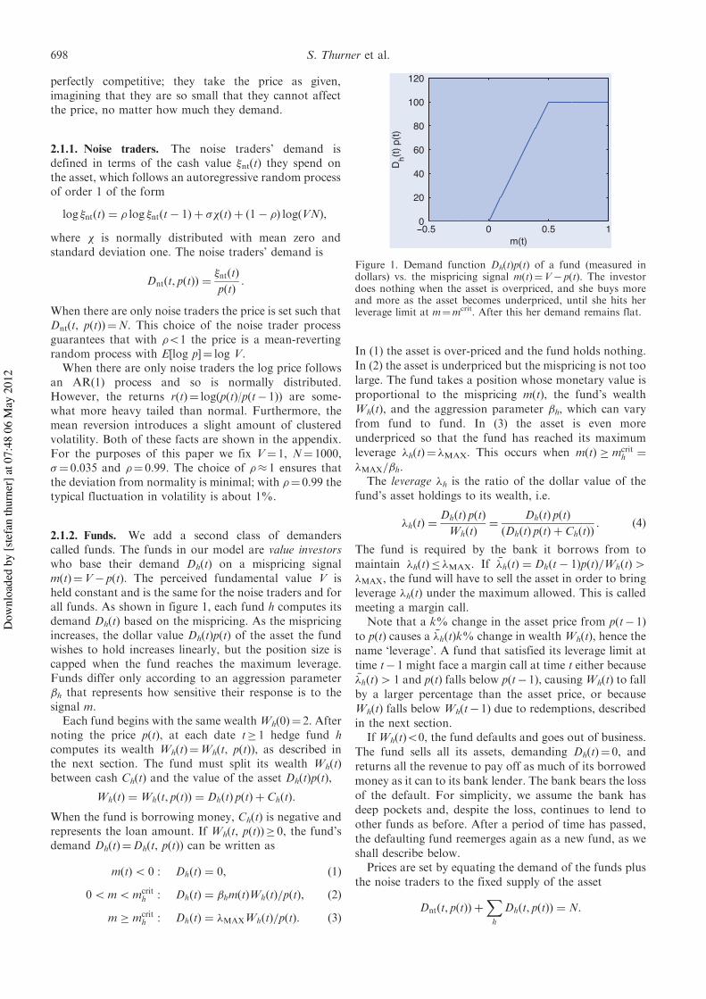
2.1.2. Funds. We add a second class of demanderscalled funds. The funds in our model are value investorswho base their demand Dh(t) on a mispricing signalm(t)"V! p(t). The perceived fundamental value V isheld constant and is the same for the noise traders and forall funds. As shown in figure 1, each fund h computes itsdemand Dh(t) based on the mispricing. As the mispricingincreases, the dollar value Dh(t)p(t) of the asset the fundwishes to hold increases linearly, but the position size iscapped when the fund reaches the maximum leverage.Funds differ only according to an aggression parameter&h that represents how sensitive their response is to thesignal m.

Each fund begins with the same wealthWh(0)" 2. Afternoting the price p(t), at each date t# 1 hedge fund hcomputes its wealth Wh(t)"Wh(t, p(t)), as described inthe next section. The fund must split its wealth Wh(t)between cash Ch(t) and the value of the asset Dh(t)p(t),

Wh$t% "Wh$t, p$t%% " Dh$t% p$t% & Ch$t%:When the fund is borrowing money, Ch(t) is negative andrepresents the loan amount. If Wh(t, p(t))# 0, the fund’sdemand Dh(t)"Dh(t, p(t)) can be written as

m$t%5 0 : Dh$t% " 0, $1%

05m5mcrith : Dh$t% " &hm$t%Wh$t%=p$t%, $2%

m # mcrith : Dh$t% " !MAXWh$t%=p$t%: $3%

In (1) the asset is over-priced and the fund holds nothing.In (2) the asset is underpriced but the mispricing is not toolarge. The fund takes a position whose monetary value isproportional to the mispricing m(t), the fund’s wealthWh(t), and the aggression parameter &h, which can varyfrom fund to fund. In (3) the asset is even moreunderpriced so that the fund has reached its maximumleverage !h(t)" !MAX. This occurs when m$t% # mcrit

h "!MAX=&h.

The leverage !h is the ratio of the dollar value of thefund’s asset holdings to its wealth, i.e.

!h$t% "Dh$t% p$t%Wh$t%

" Dh$t% p$t%$Dh$t% p$t% & Ch$t%%

: $4%

The fund is required by the bank it borrows from tomaintain !h(t)( !MAX. If !!h$t% " Dh$t! 1%p$t%=Wh$t%4!MAX, the fund will have to sell the asset in order to bringleverage !h(t) under the maximum allowed. This is calledmeeting a margin call.

Note that a k% change in the asset price from p(t! 1)to p(t) causes a !!h$t%k% change in wealth Wh(t), hence thename ‘leverage’. A fund that satisfied its leverage limit attime t! 1 might face a margin call at time t either because!!h$t%4 1 and p(t) falls below p(t! 1), causing Wh(t) to fallby a larger percentage than the asset price, or becauseWh(t) falls below Wh(t! 1) due to redemptions, describedin the next section.

If Wh(t)50, the fund defaults and goes out of business.The fund sells all its assets, demanding Dh(t)" 0, andreturns all the revenue to pay off as much of its borrowedmoney as it can to its bank lender. The bank bears the lossof the default. For simplicity, we assume the bank hasdeep pockets and, despite the loss, continues to lend toother funds as before. After a period of time has passed,the defaulting fund reemerges again as a new fund, as weshall describe below.

Prices are set by equating the demand of the funds plusthe noise traders to the fixed supply of the asset

Dnt$t, p$t%% &X

h

Dh$t, p$t%% " N:

Figure 1. Demand function Dh(t)p(t) of a fund (measured indollars) vs. the mispricing signal m(t)"V! p(t). The investordoes nothing when the asset is overpriced, and she buys moreand more as the asset becomes underpriced, until she hits herleverage limit at m"mcrit. After this her demand remains flat.


Dow

nloa

ded

by [s

tefa

n th

urne

r] a

t 07:

48 0

6 M

ay 2

012

2.2. Fund wealth dynamics

The funds’ wealth automatically grows or shrinks accord-ing to the success or failure of their trading. In addition, itchanges due to additions or withdrawals of money byinvestors, as described below. If a fund’s wealth goesbelow a critical threshold, here set to Wh(0)/10 , the fundgoes out of business,y and after a period of time, Treintro,has passed it is replaced by a new fund with wealth Wh(0)and the same parameters &h and !MAX. In the simulationswe use Treintro" 100 time steps.

A pool of fund investors, who are treated as a singlerepresentative investor, contribute or withdraw moneyfrom each fund based on a moving average of its recentperformance. This kind of behavior is well documented.z

Let

rh$t% "Dh$t! 1%$ p$t% ! p$t! 1%%

Wh$t! 1%

be the rate of return by fund h on investments at time t.The investors make their decisions about whether toinvest in the fund based on rperfh $t%, an exponential movingaverage of these performances, defined as

rperfh $t% " $1! a% rperfh $t! 1% & a rh$t%: $5%

The flow of capital in or out of the fund, Fh(t), is given by

~Fh$t% " b)rperfh $t% ! rb* )Dh$t! 1% p$t% & Ch$t! 1%*, $6%

Fh$t% " max$ ~Fh$t%, ! )Dh$t! 1% p$t% & Ch$t! 1%*%, $7%

where b is a parameter controlling how sensitive thepercentage contributions or withdrawals are to returnsand rb is the benchmark return of the investors. Theinvestors cannot take out more money than the fund has.

Funds are initially given wealth W0"Wh(0). At thebeginning of each new time step t# 1, the wealth of thefund changes according to

Wh$t% "Wh$t! 1% & ) p$t% ! p$t! 1%*Dh$t! 1% & Fh$t%:$8%

In the simulations in this paper, unless otherwise statedwe set a" 0.1, b" 0.15, rb" 0.005, and W0" 2.

The benchmark return rb plays the important role ofdetermining the relative size of hedge funds vs. noisetraders. If the benchmark return is set very low, thenfunds will become very wealthy and will buy a largequantity of the asset under even small mispricings,preventing the mispricing from ever growing large. Thiseffectively induces a hard floor on prices. If the bench-mark return is set very high, funds accumulate littlewealth and play a negligible role in price formation. Theinteresting behavior is observed at intermediate values ofrb where the funds’ demand is comparable to that of thenoise traders.

2.3. A few remarks about the model

2.3.1. Lack of short selling and its consequences. Wehave intentionally avoided short selling because shortpositions are inherently riskier than long positions. Withan unleveraged long-only position it is not possible to losemore than one owns. In contrast, with a short position itis possible to lose an arbitrarily large amount, evenwithout leverage. Because we wanted to be able to switchoff excess riskiness completely, we intentionally kept shortselling out of this model.

The disadvantage of this approach is that it makes themodel explicitly unrealistic in ways that need to be takeninto account when interpreting the results. When the assetis overpriced, long-only funds are entirely out of themarket, which can cause strong asymmetries in theproperties of prices. Since the funds normally dampexcursions from fundamentals, it can mean that thevolatility is higher when the asset is overpriced than whenit is underpriced. Mixing the two cases together wouldresult in artificially induced heavy tails and give anartificial impression of clustered volatility. The predic-tions of the model are only relevant when the asset isunderpriced and we therefore condition our analyses onthe asset being underpriced.

2.3.2. Trend following in wealth dynamics. The wealthdynamics of the funds involves a representative investorwho takes her money in or out of the fund based on itsrecent performance. We introduced this into our modelbecause it guarantees a steady-state behavior, with well-defined long-term statistical averages. Without this thewealth of the funds grows without bound, since the fundsconsistently profit at the expense of the noise traders. Thiscauses the price to eventually ‘freeze’ with the value V as afloor due to the fact that any underpricing is immediatelycorrected by the funds. Since the wealth dynamics wehave chosen is a form of trend following, it unfortunatelyintroduces some confusion about the source of the heavytails that we observe here. As we explain later, based onvarious experiments we are confident that the wealthdynamics of the investors is not the source of theheavy tails.

3. Simulation results

3.1. Wealth dynamics

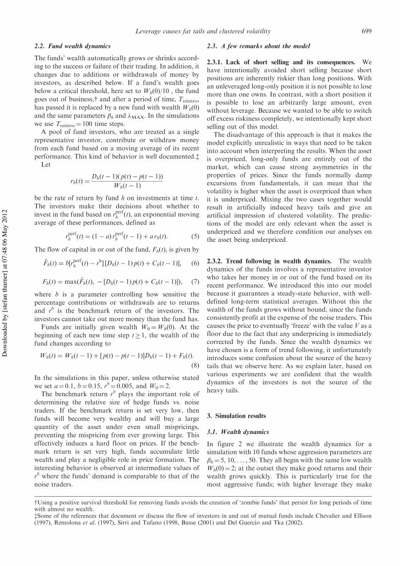
In figure 2 we illustrate the wealth dynamics for asimulation with 10 funds whose aggression parameters are&h" 5, 10, . . . , 50. They all begin with the same low wealthWh(0)" 2; at the outset they make good returns and theirwealth grows quickly. This is particularly true for themost aggressive funds; with higher leverage they make

yUsing a positive survival threshold for removing funds avoids the creation of ‘zombie funds’ that persist for long periods of timewith almost no wealth.zSome of the references that document or discuss the flow of investors in and out of mutual funds include Chevalier and Ellison(1997), Remolona et al. (1997), Sirri and Tufano (1998, Busse (2001) and Del Guercio and Tka (2002).


Dow

nloa

ded

by [s

tefa

n th

urne

r] a

t 07:

48 0

6 M

ay 2

012

higher returns so long as the asset price is increasing. Astheir wealth grows the funds have more impact, i.e. theythemselves affect prices, driving them up when they arebuying and down when they are selling. This limits theirprofit-making opportunities and imposes a ceiling ofwealth at about W" 40. There are a series of crashes thatcause defaults, particularly for the most highly leveragedfunds. Twice during the simulation, at around t" 10 000and 25 000, crashes wipe out all but the two leastaggressive funds with &h" 5 and 10. While funds&3! &10 wait to get reintroduced, fund &2 manages tobecome dominant for extended periods of time.

3.2. Returns and correlations

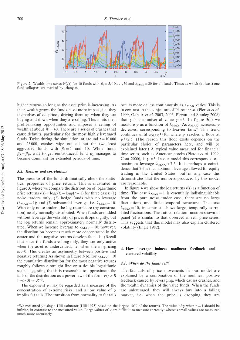
The presence of the funds dramatically alters the statis-tical properties of price returns. This is illustrated infigure 3, where we compare the distribution of logarithmicprice returns r(t)" logp(t)! logp(t! 1) for three cases: (1)noise traders only; (2) hedge funds with no leverage(!MAX" 1); and (3) substantial leverage, i.e. !MAX" 10.With only noise traders the log returns are (by construc-tion) nearly normally distributed. When funds are addedwithout leverage the volatility of prices drops slightly, butthe log returns remain approximately normally distrib-uted. When we increase leverage to !MAX" 10, however,the distribution becomes much more concentrated in thecenter and the negative returns develop fat tails. (Recallthat since the funds are long-only, they are only activewhen the asset is undervalued, i.e. when the mispricingm40. This creates an asymmetry between positive andnegative returns.) As shown in figure 3(b), for !MAX" 10the cumulative distribution for the most negative returnsroughly follows a straight line on a double logarithmicscale, suggesting that it is reasonable to approximate thetails of the distribution as a power law of the form P(r4R| m40) + R!'.

The exponent ' may be regarded as a measure of theconcentration of extreme risks, and a low value of 'implies fat tails. The transition from normality to fat tails

occurs more or less continuously as !MAX varies. This isin contrast to the conjecture of Plerou et al. (Plerou et al.1999, Gabaix et al. 2003, 2006, Plerou and Stanley 2008)that ' has a universal value '' 3. In figure 3(c) wemeasure ' as a function of !MAX. As !MAX increases, 'decreases, corresponding to heavier tails.y This trendcontinues until !MAX' 10, where ' reaches a floor at'' 2.5. (The reason this floor exists depends on theparticular choice of parameters here, and will beexplained later.) A typical value measured for financialtime series, such as American stocks (Plerou et al. 1999,Cont 2000), is '' 3. In our model this corresponds to amaximum leverage !MAX' 7.5. It is perhaps a coinci-dence that 7.5 is the maximum leverage allowed for equitytrading in the United States, but in any case thisdemonstrates that the numbers produced by this modelare reasonable.

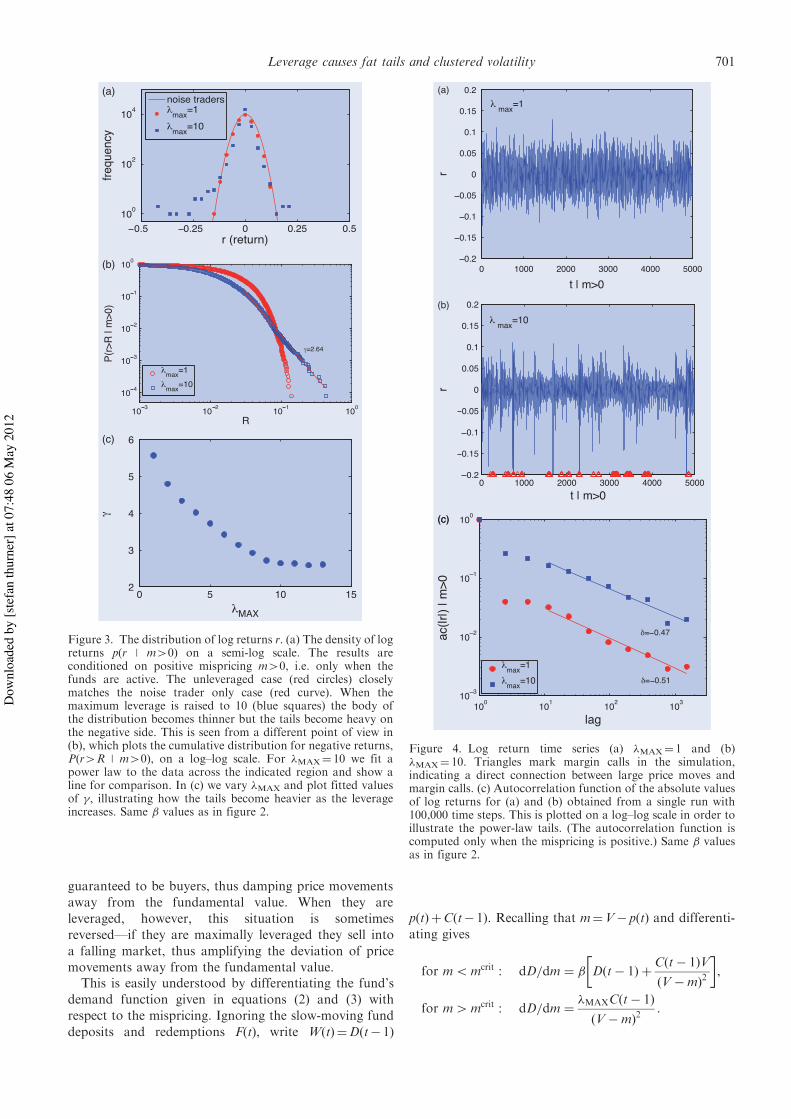
In figure 4 we show the log returns r(t) as a function oftime. The case !MAX" 1 is essentially indistinguishablefrom the pure noise trader case; there are no largefluctuations and little temporal structure. The case!MAX" 10, in contrast, shows large, temporally corre-lated fluctuations. The autocorrelation function shown inpanel (c) is similar to that observed in real price series.This suggests that this model may also explain clusteredvolatility (Engle 1982).

4. How leverage induces nonlinear feedback andclustered volatility

4.1. When do the funds sell?

The fat tails of price movements in our model areexplained by a combination of the nonlinear positivefeedback caused by leveraging, which causes crashes, andthe wealth dynamics of the value funds. When the fundsare unleveraged, they will always buy into a fallingmarket, i.e. when the price is dropping they are

Figure 2. Wealth time series Wh(t) for 10 funds with &h" 5, 10, . . . , 50 and !MAX" 20 for all funds. Times at which (at least) onefund collapses are marked by triangles.

yWe measured ' using a Hill estimator (Hill 1975) based on the largest 10% of the returns. The value of ' when !" 1 should beinfinite, in contrast to the measured value. Large values of ' are difficult to measure correctly, whereas small values are measuredmuch more accurately.


Dow

nloa

ded

by [s

tefa

n th

urne

r] a

t 07:

48 0

6 M

ay 2

012

guaranteed to be buyers, thus damping price movementsaway from the fundamental value. When they areleveraged, however, this situation is sometimesreversed—if they are maximally leveraged they sell intoa falling market, thus amplifying the deviation of pricemovements away from the fundamental value.

This is easily understood by differentiating the fund’sdemand function given in equations (2) and (3) withrespect to the mispricing. Ignoring the slow-moving funddeposits and redemptions F(t), write W(t)"D(t! 1)

p(t)&C(t! 1). Recalling that m"V! p(t) and differenti-ating gives

for m5mcrit : dD=dm " & D$t! 1% & C$t! 1%V$V!m%2

! ",

for m4mcrit : dD=dm " !MAXC$t! 1%$V!m%2

:

(a)

(b)

(c)

Figure 3. The distribution of log returns r. (a) The density of logreturns p(r | m40) on a semi-log scale. The results areconditioned on positive mispricing m40, i.e. only when thefunds are active. The unleveraged case (red circles) closelymatches the noise trader only case (red curve). When themaximum leverage is raised to 10 (blue squares) the body ofthe distribution becomes thinner but the tails become heavy onthe negative side. This is seen from a different point of view in(b), which plots the cumulative distribution for negative returns,P(r4R | m40), on a log–log scale. For !MAX" 10 we fit apower law to the data across the indicated region and show aline for comparison. In (c) we vary !MAX and plot fitted valuesof ', illustrating how the tails become heavier as the leverageincreases. Same & values as in figure 2.

Figure 4. Log return time series (a) !MAX" 1 and (b)!MAX" 10. Triangles mark margin calls in the simulation,indicating a direct connection between large price moves andmargin calls. (c) Autocorrelation function of the absolute valuesof log returns for (a) and (b) obtained from a single run with100,000 time steps. This is plotted on a log–log scale in order toillustrate the power-law tails. (The autocorrelation function iscomputed only when the mispricing is positive.) Same & valuesas in figure 2.


Dow

nloa

ded

by [s

tefa

n th

urne

r] a

t 07:

48 0

6 M

ay 2

012

As long as the fund always remains unleveraged, the cashC(t! 1) is always positive and the derivative of thedemand with the mispricing is always positive. Thismeans the fund always buys as the price is falling. Incontrast, when the fund is leveraged, then C(t! 1) isnegative. This means that the fund is always selling as theprice is falling when it is above its leverage limit, anddepending on the circumstances, it may start selling evenbefore then.

To visualize this more clearly, consider the derivative atthe value of the mispricing at the last period,m"V! p(t! 1). At that point, ignoring redemptions,we can assume that D(t! 1) and C(t! 1) are chosen sothat for m5mcrit the fraction of the wealth held in theasset is Dp/W"&m and the fraction held in cash isC/W" 1! &m. Similarly, if the fund is over its leveragelimit we can assume that the fraction of the wealth held inthe asset is Dp/W" !MAX, and the fraction held is cash isC/W" 1! !MAX. This implies that the rate of buying orselling under an infinitesimal change in the mispricingfrom the last period is

for m5mcrit :dD=dm

W" &$V! &m

2%$V!m%2

,

for m4mcrit :dD=dm

W" !MAX$1! !MAX%

$V!m%2:

When the fund is leveraged, then 1! !MAX50, and thesecond term is negative, so when m4mcrit the fund alwayssells as the mispricing increases. If &m24V, then the fundmay sell as the mispricing increases even when m5mcrit.

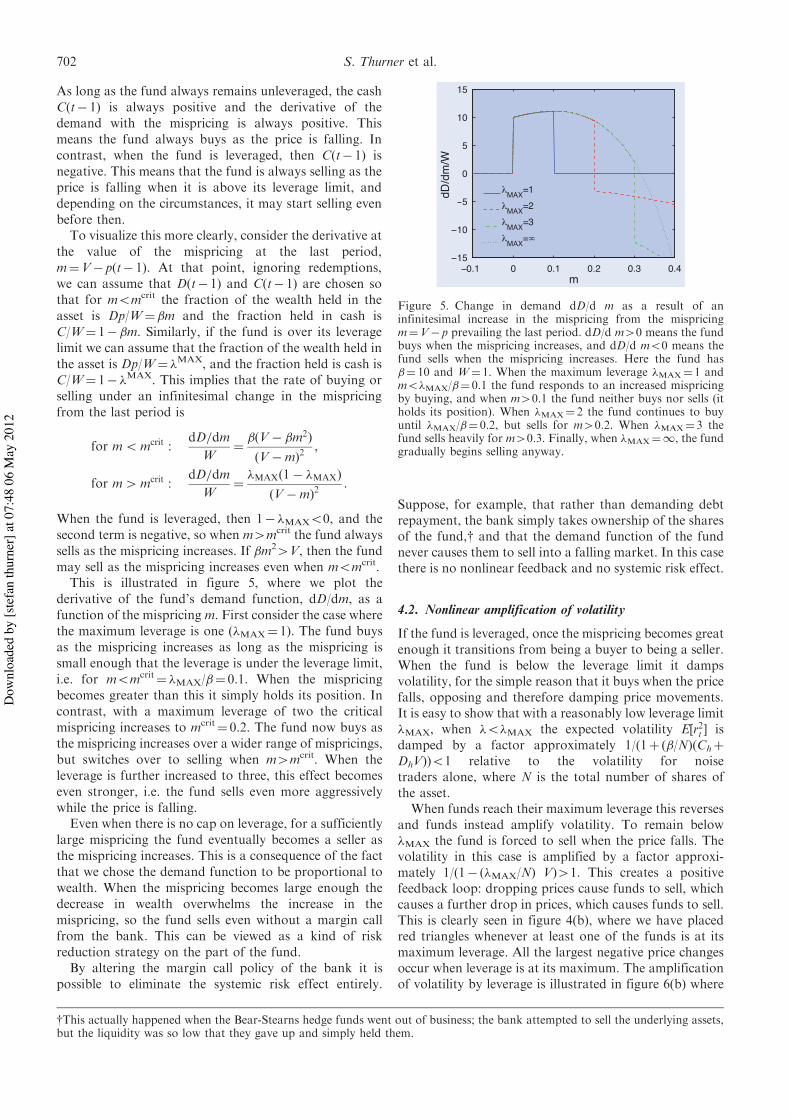
This is illustrated in figure 5, where we plot thederivative of the fund’s demand function, dD/dm, as afunction of the mispricing m. First consider the case wherethe maximum leverage is one (!MAX" 1). The fund buysas the mispricing increases as long as the mispricing issmall enough that the leverage is under the leverage limit,i.e. for m5mcrit" !MAX/&" 0.1. When the mispricingbecomes greater than this it simply holds its position. Incontrast, with a maximum leverage of two the criticalmispricing increases to mcrit" 0.2. The fund now buys asthe mispricing increases over a wider range of mispricings,but switches over to selling when m4mcrit. When theleverage is further increased to three, this effect becomeseven stronger, i.e. the fund sells even more aggressivelywhile the price is falling.

Even when there is no cap on leverage, for a sufficientlylarge mispricing the fund eventually becomes a seller asthe mispricing increases. This is a consequence of the factthat we chose the demand function to be proportional towealth. When the mispricing becomes large enough thedecrease in wealth overwhelms the increase in themispricing, so the fund sells even without a margin callfrom the bank. This can be viewed as a kind of riskreduction strategy on the part of the fund.

By altering the margin call policy of the bank it ispossible to eliminate the systemic risk effect entirely.

Suppose, for example, that rather than demanding debtrepayment, the bank simply takes ownership of the sharesof the fund,y and that the demand function of the fundnever causes them to sell into a falling market. In this casethere is no nonlinear feedback and no systemic risk effect.

4.2. Nonlinear amplification of volatility

If the fund is leveraged, once the mispricing becomes greatenough it transitions from being a buyer to being a seller.When the fund is below the leverage limit it dampsvolatility, for the simple reason that it buys when the pricefalls, opposing and therefore damping price movements.It is easy to show that with a reasonably low leverage limit!MAX, when !5!MAX the expected volatility E)r2t * isdamped by a factor approximately 1/(1& (&/N)(Ch&DhV))51 relative to the volatility for noisetraders alone, where N is the total number of shares ofthe asset.

When funds reach their maximum leverage this reversesand funds instead amplify volatility. To remain below!MAX the fund is forced to sell when the price falls. Thevolatility in this case is amplified by a factor approxi-mately 1/(1! (!MAX/N) V)41. This creates a positivefeedback loop: dropping prices cause funds to sell, whichcauses a further drop in prices, which causes funds to sell.This is clearly seen in figure 4(b), where we have placedred triangles whenever at least one of the funds is at itsmaximum leverage. All the largest negative price changesoccur when leverage is at its maximum. The amplificationof volatility by leverage is illustrated in figure 6(b) where

Figure 5. Change in demand dD/d m as a result of aninfinitesimal increase in the mispricing from the mispricingm"V! p prevailing the last period. dD/d m40 means the fundbuys when the mispricing increases, and dD/d m50 means thefund sells when the mispricing increases. Here the fund has&" 10 and W" 1. When the maximum leverage !MAX" 1 andm5!MAX/&" 0.1 the fund responds to an increased mispricingby buying, and when m40.1 the fund neither buys nor sells (itholds its position). When !MAX" 2 the fund continues to buyuntil !MAX/&" 0.2, but sells for m40.2. When !MAX" 3 thefund sells heavily for m40.3. Finally, when !MAX"1, the fundgradually begins selling anyway.

yThis actually happened when the Bear-Stearns hedge funds went out of business; the bank attempted to sell the underlying assets,but the liquidity was so low that they gave up and simply held them.


Dow

nloa

ded

by [s

tefa

n th

urne

r] a

t 07:

48 0

6 M

ay 2

012

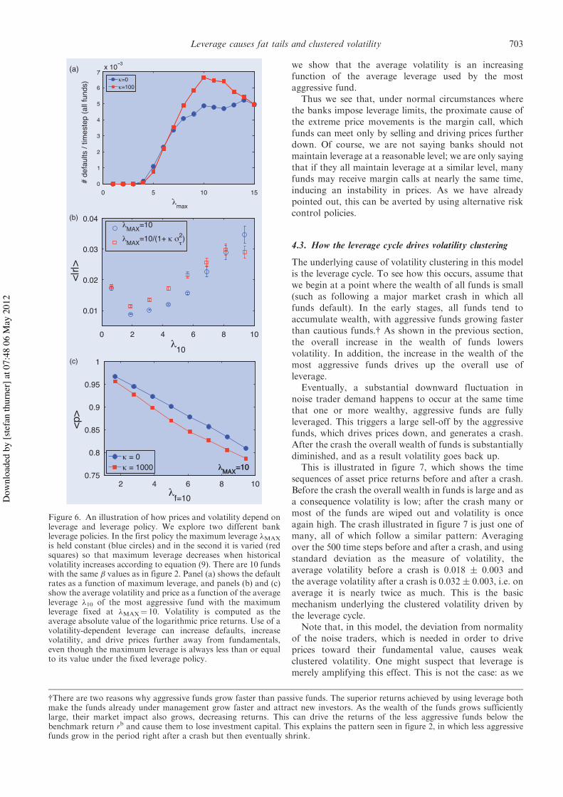
we show that the average volatility is an increasingfunction of the average leverage used by the mostaggressive fund.

Thus we see that, under normal circumstances wherethe banks impose leverage limits, the proximate cause ofthe extreme price movements is the margin call, whichfunds can meet only by selling and driving prices furtherdown. Of course, we are not saying banks should notmaintain leverage at a reasonable level; we are only sayingthat if they all maintain leverage at a similar level, manyfunds may receive margin calls at nearly the same time,inducing an instability in prices. As we have alreadypointed out, this can be averted by using alternative riskcontrol policies.

4.3. How the leverage cycle drives volatility clustering

The underlying cause of volatility clustering in this modelis the leverage cycle. To see how this occurs, assume thatwe begin at a point where the wealth of all funds is small(such as following a major market crash in which allfunds default). In the early stages, all funds tend toaccumulate wealth, with aggressive funds growing fasterthan cautious funds.y As shown in the previous section,the overall increase in the wealth of funds lowersvolatility. In addition, the increase in the wealth of themost aggressive funds drives up the overall use ofleverage.

Eventually, a substantial downward fluctuation innoise trader demand happens to occur at the same timethat one or more wealthy, aggressive funds are fullyleveraged. This triggers a large sell-off by the aggressivefunds, which drives prices down, and generates a crash.After the crash the overall wealth of funds is substantiallydiminished, and as a result volatility goes back up.

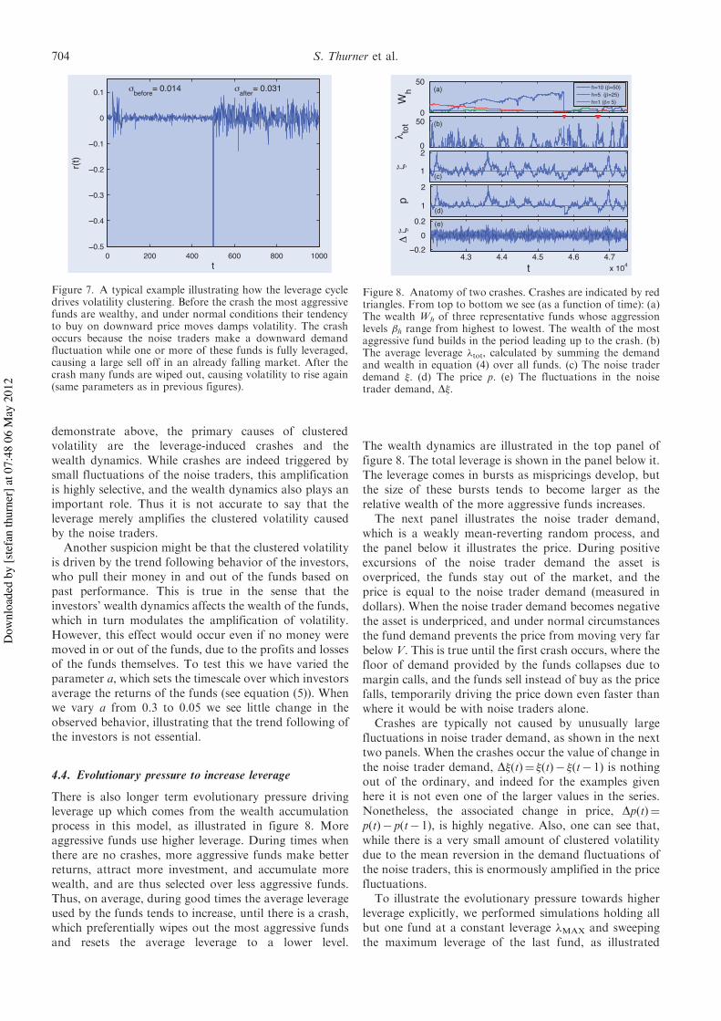
This is illustrated in figure 7, which shows the timesequences of asset price returns before and after a crash.Before the crash the overall wealth in funds is large and asa consequence volatility is low; after the crash many ormost of the funds are wiped out and volatility is onceagain high. The crash illustrated in figure 7 is just one ofmany, all of which follow a similar pattern: Averagingover the 500 time steps before and after a crash, and usingstandard deviation as the measure of volatility, theaverage volatility before a crash is 0.018 , 0.003 andthe average volatility after a crash is 0.032 , 0.003, i.e. onaverage it is nearly twice as much. This is the basicmechanism underlying the clustered volatility driven bythe leverage cycle.

Note that, in this model, the deviation from normalityof the noise traders, which is needed in order to driveprices toward their fundamental value, causes weakclustered volatility. One might suspect that leverage ismerely amplifying this effect. This is not the case: as we

(a)

(b)

(c)

Figure 6. An illustration of how prices and volatility depend onleverage and leverage policy. We explore two different bankleverage policies. In the first policy the maximum leverage !MAX

is held constant (blue circles) and in the second it is varied (redsquares) so that maximum leverage decreases when historicalvolatility increases according to equation (9). There are 10 fundswith the same & values as in figure 2. Panel (a) shows the defaultrates as a function of maximum leverage, and panels (b) and (c)show the average volatility and price as a function of the averageleverage !10 of the most aggressive fund with the maximumleverage fixed at !MAX" 10. Volatility is computed as theaverage absolute value of the logarithmic price returns. Use of avolatility-dependent leverage can increase defaults, increasevolatility, and drive prices further away from fundamentals,even though the maximum leverage is always less than or equalto its value under the fixed leverage policy.

yThere are two reasons why aggressive funds grow faster than passive funds. The superior returns achieved by using leverage bothmake the funds already under management grow faster and attract new investors. As the wealth of the funds grows sufficientlylarge, their market impact also grows, decreasing returns. This can drive the returns of the less aggressive funds below thebenchmark return rb and cause them to lose investment capital. This explains the pattern seen in figure 2, in which less aggressivefunds grow in the period right after a crash but then eventually shrink.


Dow

nloa

ded

by [s

tefa

n th

urne

r] a

t 07:

48 0

6 M

ay 2

012

demonstrate above, the primary causes of clusteredvolatility are the leverage-induced crashes and thewealth dynamics. While crashes are indeed triggered bysmall fluctuations of the noise traders, this amplificationis highly selective, and the wealth dynamics also plays animportant role. Thus it is not accurate to say that theleverage merely amplifies the clustered volatility causedby the noise traders.

Another suspicion might be that the clustered volatilityis driven by the trend following behavior of the investors,who pull their money in and out of the funds based onpast performance. This is true in the sense that theinvestors’ wealth dynamics affects the wealth of the funds,which in turn modulates the amplification of volatility.However, this effect would occur even if no money weremoved in or out of the funds, due to the profits and lossesof the funds themselves. To test this we have varied theparameter a, which sets the timescale over which investorsaverage the returns of the funds (see equation (5)). Whenwe vary a from 0.3 to 0.05 we see little change in theobserved behavior, illustrating that the trend following ofthe investors is not essential.

4.4. Evolutionary pressure to increase leverage

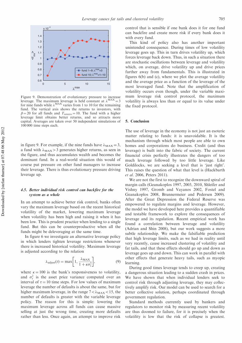
There is also longer term evolutionary pressure drivingleverage up which comes from the wealth accumulationprocess in this model, as illustrated in figure 8. Moreaggressive funds use higher leverage. During times whenthere are no crashes, more aggressive funds make betterreturns, attract more investment, and accumulate morewealth, and are thus selected over less aggressive funds.Thus, on average, during good times the average leverageused by the funds tends to increase, until there is a crash,which preferentially wipes out the most aggressive fundsand resets the average leverage to a lower level.

The wealth dynamics are illustrated in the top panel offigure 8. The total leverage is shown in the panel below it.The leverage comes in bursts as mispricings develop, butthe size of these bursts tends to become larger as therelative wealth of the more aggressive funds increases.

The next panel illustrates the noise trader demand,which is a weakly mean-reverting random process, andthe panel below it illustrates the price. During positiveexcursions of the noise trader demand the asset isoverpriced, the funds stay out of the market, and theprice is equal to the noise trader demand (measured indollars). When the noise trader demand becomes negativethe asset is underpriced, and under normal circumstancesthe fund demand prevents the price from moving very farbelow V. This is true until the first crash occurs, where thefloor of demand provided by the funds collapses due tomargin calls, and the funds sell instead of buy as the pricefalls, temporarily driving the price down even faster thanwhere it would be with noise traders alone.

Crashes are typically not caused by unusually largefluctuations in noise trader demand, as shown in the nexttwo panels. When the crashes occur the value of change inthe noise trader demand, D"(t)" "(t)! "(t! 1) is nothingout of the ordinary, and indeed for the examples givenhere it is not even one of the larger values in the series.Nonetheless, the associated change in price, Dp(t)"p(t)! p(t! 1), is highly negative. Also, one can see that,while there is a very small amount of clustered volatilitydue to the mean reversion in the demand fluctuations ofthe noise traders, this is enormously amplified in the pricefluctuations.

To illustrate the evolutionary pressure towards higherleverage explicitly, we performed simulations holding allbut one fund at a constant leverage !MAX and sweepingthe maximum leverage of the last fund, as illustrated

Figure 7. A typical example illustrating how the leverage cycledrives volatility clustering. Before the crash the most aggressivefunds are wealthy, and under normal conditions their tendencyto buy on downward price moves damps volatility. The crashoccurs because the noise traders make a downward demandfluctuation while one or more of these funds is fully leveraged,causing a large sell off in an already falling market. After thecrash many funds are wiped out, causing volatility to rise again(same parameters as in previous figures).

Figure 8. Anatomy of two crashes. Crashes are indicated by redtriangles. From top to bottom we see (as a function of time): (a)The wealth Wh of three representative funds whose aggressionlevels &h range from highest to lowest. The wealth of the mostaggressive fund builds in the period leading up to the crash. (b)The average leverage !tot, calculated by summing the demandand wealth in equation (4) over all funds. (c) The noise traderdemand ". (d) The price p. (e) The fluctuations in the noisetrader demand, D".


Dow

nloa

ded

by [s

tefa

n th

urne

r] a

t 07:

48 0

6 M

ay 2

012

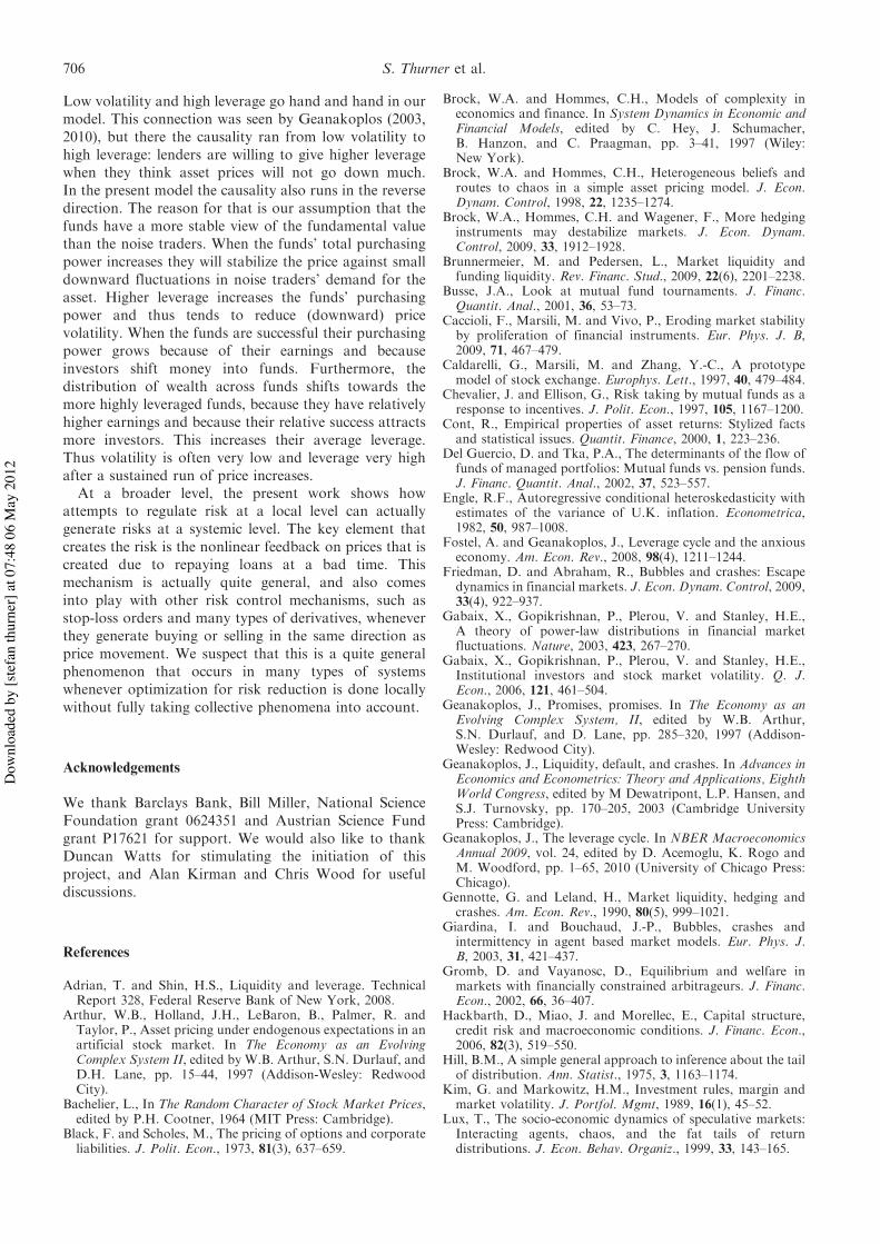
in figure 9. For example, if the nine funds have !MAX" 3,a fund with !MAX43 generates higher returns, as seen inthe figure, and thus accumulates wealth and becomes thedominant fund. In a real-world situation this would ofcourse put pressure on other fund managers to increasetheir leverage. There is thus evolutionary pressure drivingleverage up.

4.5. Better individual risk control can backfire for thesystem as a whole

In an attempt to achieve better risk control, banks oftenvary the maximum leverage based on the recent historicalvolatility of the market, lowering maximum leveragewhen volatility has been high and raising it when it hasbeen low. This is prudent practice when lending to a singlefund. But this can be counterproductive when all thefunds might be deleveraging at the same time.

In figure 6 we investigate an alternative leverage policyin which lenders tighten leverage restrictions wheneverthere is increased historical volatility. Maximum leverageis adjusted according to the relation

!adjust$t% " max 1,!MAX

1& ($2)

! ", $9%

where (" 100 is the bank’s responsiveness to volatility,and $2) is the asset price variance computed over aninterval of )" 10 time steps. For low values of maximumleverage the number of defaults is about the same, but forhigher maximum leverage, in the range 75!MAX515, thenumber of defaults is greater with the variable leveragepolicy. The reason for this is simple: lowering themaximum leverage across all funds can cause massiveselling at just the wrong time, creating more defaultsrather than less. Once again, an attempt to improve risk

control that is sensible if one bank does it for one fundcan backfire and create more risk if every bank does itwith every fund.

This kind of policy also has another importantunintended consequence. During times of low volatilityleverage goes up. This in turn drives volatility up, whichforces leverage back down. Thus, in such a situation thereare stochastic oscillations between leverage and volatilitywhich, on average, drive volatility up and drive pricesfurther away from fundamentals. This is illustrated infigures 6(b) and (c), where we plot the average volatilityand the average price as a function of the leverage of themost leveraged fund. Note that the amplification ofvolatility occurs even though, under the variable maxi-mum leverage risk control protocol, the maximumvolatility is always less than or equal to its value underthe fixed protocol.

5. Conclusion

The use of leverage in the economy is not just an esotericmatter relating to funds: it is unavoidable. It is themechanism through which most people are able to ownhomes and corporations do business. Credit (and thusleverage) is built into the fabric of society. The currentfinancial crisis perfectly illustrates the dangers of toomuch leverage followed by too little leverage. LikeGoldilocks, we are seeking a level that is ‘just right’.This raises the question of what that level is (Hackbarthet al. 2006, Peters 2011).

We are not the first to recognize the downward spiral ofmargin calls (Geanakoplos 1997, 2003, 2010, Shleifer andVishny 1997, Gromb and Vayanos 2002, Fostel andGeanakoplos 2008, Brunnermeier and Pedersen 2009).After the Great Depression the Federal Reserve wasempowered to regulate margins and leverage. However,the model we have developed here provides a quantifiableand testable framework to explore the consequences ofleverage and its regulation. Recent empirical work hasfound a correlation between leverage and volatility(Adrian and Shin 2008), but our work suggests a moresubtle relationship. We make the falsifiable predictionthat high leverage limits, such as we had in reality untilvery recently, cause increased clustering of volatility andfat tails, and that these effects should go up and down asleverage goes up and down. This can work in parallel withother effects that generate heavy tails, such as myopiclearning.

During good times leverage tends to creep up, creatinga dangerous situation leading to a sudden crash in prices.We have shown that when individual lenders seek tocontrol risk through adjusting leverage, they may collec-tively amplify risk. Our model can be used to search for abetter collective solution, perhaps coordinated throughgovernment regulation.

Standard methods currently used by bankers andregulators to monitor risk by measuring recent volatilityare thus doomed to failure, for it is precisely when thevolatility is low that the risk of collapse is greatest.

Figure 9. Demonstration of evolutionary pressure to increaseleverage. The maximum leverage is held constant at !MAX" 3for nine funds while !MAX varies from 1 to 10 for the remainingfund. The vertical axis shows the returns to investors, with&" 20 for all funds and Treintro" 10. The fund with a higherleverage limit obtains better returns, and so attracts morecapital. Averages are taken over 50 independent simulations of100 000 time steps each.


Dow

nloa

ded

by [s

tefa

n th

urne

r] a

t 07:

48 0

6 M

ay 2

012

Low volatility and high leverage go hand and hand in ourmodel. This connection was seen by Geanakoplos (2003,2010), but there the causality ran from low volatility tohigh leverage: lenders are willing to give higher leveragewhen they think asset prices will not go down much.In the present model the causality also runs in the reversedirection. The reason for that is our assumption that thefunds have a more stable view of the fundamental valuethan the noise traders. When the funds’ total purchasingpower increases they will stabilize the price against smalldownward fluctuations in noise traders’ demand for theasset. Higher leverage increases the funds’ purchasingpower and thus tends to reduce (downward) pricevolatility. When the funds are successful their purchasingpower grows because of their earnings and becauseinvestors shift money into funds. Furthermore, thedistribution of wealth across funds shifts towards themore highly leveraged funds, because they have relativelyhigher earnings and because their relative success attractsmore investors. This increases their average leverage.Thus volatility is often very low and leverage very highafter a sustained run of price increases.

At a broader level, the present work shows howattempts to regulate risk at a local level can actuallygenerate risks at a systemic level. The key element thatcreates the risk is the nonlinear feedback on prices that iscreated due to repaying loans at a bad time. Thismechanism is actually quite general, and also comesinto play with other risk control mechanisms, such asstop-loss orders and many types of derivatives, wheneverthey generate buying or selling in the same direction asprice movement. We suspect that this is a quite generalphenomenon that occurs in many types of systemswhenever optimization for risk reduction is done locallywithout fully taking collective phenomena into account.

Acknowledgements

We thank Barclays Bank, Bill Miller, National ScienceFoundation grant 0624351 and Austrian Science Fundgrant P17621 for support. We would also like to thankDuncan Watts for stimulating the initiation of thisproject, and Alan Kirman and Chris Wood for usefuldiscussions.

References

Adrian, T. and Shin, H.S., Liquidity and leverage. TechnicalReport 328, Federal Reserve Bank of New York, 2008.

Arthur, W.B., Holland, J.H., LeBaron, B., Palmer, R. andTaylor, P., Asset pricing under endogenous expectations in anartificial stock market. In The Economy as an EvolvingComplex System II, edited by W.B. Arthur, S.N. Durlauf, andD.H. Lane, pp. 15–44, 1997 (Addison-Wesley: RedwoodCity).

Bachelier, L., In The Random Character of Stock Market Prices,edited by P.H. Cootner, 1964 (MIT Press: Cambridge).

Black, F. and Scholes, M., The pricing of options and corporateliabilities. J. Polit. Econ., 1973, 81(3), 637–659.

Brock, W.A. and Hommes, C.H., Models of complexity ineconomics and finance. In System Dynamics in Economic andFinancial Models, edited by C. Hey, J. Schumacher,B. Hanzon, and C. Praagman, pp. 3–41, 1997 (Wiley:New York).

Brock, W.A. and Hommes, C.H., Heterogeneous beliefs androutes to chaos in a simple asset pricing model. J. Econ.Dynam. Control, 1998, 22, 1235–1274.

Brock, W.A., Hommes, C.H. and Wagener, F., More hedginginstruments may destabilize markets. J. Econ. Dynam.Control, 2009, 33, 1912–1928.

Brunnermeier, M. and Pedersen, L., Market liquidity andfunding liquidity. Rev. Financ. Stud., 2009, 22(6), 2201–2238.

Busse, J.A., Look at mutual fund tournaments. J. Financ.Quantit. Anal., 2001, 36, 53–73.

Caccioli, F., Marsili, M. and Vivo, P., Eroding market stabilityby proliferation of financial instruments. Eur. Phys. J. B,2009, 71, 467–479.

Caldarelli, G., Marsili, M. and Zhang, Y.-C., A prototypemodel of stock exchange. Europhys. Lett., 1997, 40, 479–484.

Chevalier, J. and Ellison, G., Risk taking by mutual funds as aresponse to incentives. J. Polit. Econ., 1997, 105, 1167–1200.

Cont, R., Empirical properties of asset returns: Stylized factsand statistical issues. Quantit. Finance, 2000, 1, 223–236.

Del Guercio, D. and Tka, P.A., The determinants of the flow offunds of managed portfolios: Mutual funds vs. pension funds.J. Financ. Quantit. Anal., 2002, 37, 523–557.

Engle, R.F., Autoregressive conditional heteroskedasticity withestimates of the variance of U.K. inflation. Econometrica,1982, 50, 987–1008.

Fostel, A. and Geanakoplos, J., Leverage cycle and the anxiouseconomy. Am. Econ. Rev., 2008, 98(4), 1211–1244.

Friedman, D. and Abraham, R., Bubbles and crashes: Escapedynamics in financial markets. J. Econ. Dynam. Control, 2009,33(4), 922–937.

Gabaix, X., Gopikrishnan, P., Plerou, V. and Stanley, H.E.,A theory of power-law distributions in financial marketfluctuations. Nature, 2003, 423, 267–270.

Gabaix, X., Gopikrishnan, P., Plerou, V. and Stanley, H.E.,Institutional investors and stock market volatility. Q. J.Econ., 2006, 121, 461–504.

Geanakoplos, J., Promises, promises. In The Economy as anEvolving Complex System, II, edited by W.B. Arthur,S.N. Durlauf, and D. Lane, pp. 285–320, 1997 (Addison-Wesley: Redwood City).

Geanakoplos, J., Liquidity, default, and crashes. In Advances inEconomics and Econometrics: Theory and Applications, EighthWorld Congress, edited by M Dewatripont, L.P. Hansen, andS.J. Turnovsky, pp. 170–205, 2003 (Cambridge UniversityPress: Cambridge).

Geanakoplos, J., The leverage cycle. In NBER MacroeconomicsAnnual 2009, vol. 24, edited by D. Acemoglu, K. Rogo andM. Woodford, pp. 1–65, 2010 (University of Chicago Press:Chicago).

Gennotte, G. and Leland, H., Market liquidity, hedging andcrashes. Am. Econ. Rev., 1990, 80(5), 999–1021.

Giardina, I. and Bouchaud, J.-P., Bubbles, crashes andintermittency in agent based market models. Eur. Phys. J.B, 2003, 31, 421–437.

Gromb, D. and Vayanosc, D., Equilibrium and welfare inmarkets with financially constrained arbitrageurs. J. Financ.Econ., 2002, 66, 36–407.

Hackbarth, D., Miao, J. and Morellec, E., Capital structure,credit risk and macroeconomic conditions. J. Financ. Econ.,2006, 82(3), 519–550.

Hill, B.M., A simple general approach to inference about the tailof distribution. Ann. Statist., 1975, 3, 1163–1174.

Kim, G. and Markowitz, H.M., Investment rules, margin andmarket volatility. J. Portfol. Mgmt, 1989, 16(1), 45–52.

Lux, T., The socio-economic dynamics of speculative markets:Interacting agents, chaos, and the fat tails of returndistributions. J. Econ. Behav. Organiz., 1999, 33, 143–165.


Dow

nloa

ded

by [s

tefa

n th

urne

r] a

t 07:

48 0

6 M

ay 2

012

Lux, T. and Marchesi, M., Scaling and criticality in a stochasticmulti-agent model of a financial market. Nature, 1999, 397,498–500.

Mandelbrot, B.B., The variation of certain speculative prices.J. Business, 1963, 36, 394–419.

Palmer, R., Arthur, W.B., Holland, J.H., LeBaron, B. andTaylor, P., Artificial economic life: A simple model of a stockmarket. Physica D, 1994, 75, 264–274.

Peters, O., Optimal leverage from non-ergodicity. Quantit.Finance, 2011, 11, 1593–1602.

Plerou, V., Gopikrishnan, P., Nunes Amaral, L.A., Meyer, M.and Stanley, H.E., Scaling of the distribution of pricefluctuations of individual companies. Phys. Rev. E, 1999,60, 6519–6529.

Plerou, V. and Stanley, H.E., Stock return distributions: Tests ofscaling and universality from three distinct stock markets.Phys. Rev. E, 2008, 77, 037101.

Remolona, E.M., Kleiman, P. and Gruenstein, D., Marketreturns and mutual fund flows. FRBNY Econ. Policy Rev.,1997, 33–52.

Shleifer, A. and Vishny, R.W., The limits of arbitrage. J.Finance, 1997, 52, 35–55.

Sirri, E.R. and Tufano, P., Costly search and mutual fund flows.J. Finance, 1998, 53, 1589–1622.

Appendix A: Properties of the noise trader process

In this appendix we show that, for the parameters we usehere, the noise trader process by itself has slightly non-normal returns and weak clustered volatility. Assume nofunds, so that the dynamics are determined solely by thenoise traders. For convenience make the change of

notation yt" log "(t), and for convenience let V"N" 1(which only shifts the mean). The price is given byDnt" "(t)/p(t)"N" 1 and the log price is log p(t)" log"(t)" y(t). The price dynamics become

y$t& 1% " #y$t% & $%$t& 1%: $A1%

The noise %(t) is normally distributed with zero mean. Thereturn r(t) is

r$t& 1% " y$t& 1% ! y$t% " $#! 1% y$t% & $%$t& 1%: $A2%

Squaring this and averaging gives

E)r$t%2 j y$t%* " $#! 1%2y$t%2 & $2:

Thus the volatility varies conditionally on y(t), implyingthat there is some clustered volatility even when onlynoise traders are present. An estimate of the typical size ofy(t)2 can be made by squaring equation (A1) and makinguse of stationarity, which yields E[y(t)2]" $2/(1! #)2.Substituting in equation (A2) gives a typical relativevariation in volatility of (1! #)2/(1! #2), which for#" 0.99 is about 0.005. Thus the variation in volatilityfor the pure noise trader process is small for theparameters we use here, and vanishes in the limit #! 1.The fact that the variance fluctuates means that the timeseries r(t) is not identically distributed, and the marginaldistribution P(r) is a Gaussian mixture, which is slightlymore heavy-tailed than a normal distribution.


Dow

nloa

ded

by [s

tefa

n th

urne

r] a

t 07:

48 0

6 M

ay 2

012

leverage causes fat tails and clustered volatility · pdf fileleverage causes fat tails and...

Documents