lf-net: learning local features from images
TRANSCRIPT

LF-Net: Learning Local Features from Images
Yuki OnoSony Imaging Products & Solutions Inc.
Eduard TrullsÉcole Polytechnique Fédérale de Lausanne
Pascal FuaÉcole Polytechnique Fédérale de Lausanne
Kwang Moo YiVisual Computing Group, University of Victoria
Abstract
We present a novel deep architecture and a training strategy to learn a local featurepipeline from scratch, using collections of images without the need for humansupervision. To do so we exploit depth and relative camera pose cues to create avirtual target that the network should achieve on one image, provided the outputs ofthe network for the other image. While this process is inherently non-differentiable,we show that we can optimize the network in a two-branch setup by confining it toone branch, while preserving differentiability in the other. We train our method onboth indoor and outdoor datasets, with depth data from 3D sensors for the former,and depth estimates from an off-the-shelf Structure-from-Motion solution for thelatter. Our models outperform the state of the art on sparse feature matching onboth datasets, while running at 60+ fps for QVGA images.
1 Introduction
Establishing correspondences across images is at the heart of many Computer Vision algorithms,such as those for wide-baseline stereo, object detection, and image retrieval. With the emergenceof SIFT [23], sparse methods that find interest points and then match them across images becamethe de facto standard. In recent years, many of these approaches have been revisited using deepnets [11, 33, 48, 49], which has also sparked a revival for dense matching [9, 43, 45, 52, 53].
However, dense methods tend to fail in complex scenes with occlusions [49], while sparse methodsstill suffer from severe limitations. Some can only train individual parts of the feature extractionpipeline [33] while others can be trained end-to-end but still require the output of hand-crafteddetectors to initialize the training process [11, 48, 49]. For the former, reported gains in performancemay fade away when they are integrated into the full pipeline. For the latter, parts of the image whichhand-crafted detectors miss are simply discarded for training.
In this paper, we propose a sparse-matching method with a novel deep architecture, which wename LF-Net, for Local Feature Network, that is trainable end-to-end and does not require usinga hand-crafted detector to generate training data. Instead, we use image pairs for which we knowthe relative pose and corresponding depth maps, which can be obtained either with laser scanners orshape-from-structure algorithms [34], without any further annotation.
Being thus given dense correspondence data, we could train a feature extraction pipeline by selectinga number of keypoints over two images, computing descriptors for each keypoint, using the groundtruth to determine which ones match correctly across images, and use those to learn good descriptors.This is, however, not feasible in practice. First, extracting multiple maxima from a score map isinherently not differentiable. Second, performing this operation over each image produces two
32nd Conference on Neural Information Processing Systems (NIPS 2018), Montréal, Canada.
arX
iv:1
805.
0966
2v2
[cs
.CV
] 2
2 N
ov 2
018

disjoint sets of keypoints which will typically produce very few ground truth matches, which we needto train the descriptor network, and in turn guide the detector towards keypoints which are distinctiveand good for matching.
We therefore propose to create a virtual target response for the network, using the ground-truthgeometry in a non-differentiable way. Specifically, we run our detector on the first image, find themaxima, and then optimize the weights so that when run on the second image it produces a cleanresponse map with sharp maxima at the right locations. Moreover, we warp the keypoints selectedin this manner to the other image using the ground truth, guaranteeing a large pool of ground truthmatches. Note that while we break differentiability in one branch, the other one can be trained end toend, which lets us learn discriminative features by learning the entire pipeline at once. We show thatour method greatly outperforms the state-of-the-art.
2 Related work
Since the appearance of SIFT [23], local features have played a crucial role in computer vision,becoming the de facto standard for wide-baseline image matching [14]. They are versatile [23, 29, 47]and remain useful in many scenarios. This remains true even in competition with deep networkalternatives, which typically involve dense matching [9, 43, 45, 52, 53] and tend to work best onnarrow baselines, as they can suffer from occlusions, which local features are robust against.
Typically, feature extraction and matching comprises three stages: finding interest points, estimatingtheir orientation, and creating a descriptor for each. SIFT [23], along with more recent methods [1,5, 32, 48] implements the entire pipeline. However, many other approaches target some of theirindividual components, be it feature point extraction [31, 44], orientation estimation [50], or descriptorgeneration [36, 40, 41]. One problem with this approach is that increasing the performance of onecomponent does not necessarily translate into overall improvements [35, 48].
Next, we briefly introduce some representative algorithms below, separating those that rely onhand-crafted features from those that use Machine Learning techniques extensively.
Hand-crafted. SIFT [23] was the first widely successful attempt at designing an integrated solu-tion for local feature extraction. Many subsequent efforts focused on reducing its computationalrequirements. For instance, SURF [5] used Haar filters and integral images for fast keypoint detectionand descriptor extraction. DAISY [41] computed dense descriptors efficiently from convolutions oforiented gradient maps. The literature on this topic is very extensive—we refer the reader to [28].
Learned. While methods such as FAST [30] used machine learning techniques to extract keypoints,most early efforts in this area targeted descriptors, e.g.using metric learning [38] or convex opti-mization [37]. However, with the advent of deep learning, there has been a renewed push towardsreplacing all the components of the standard pipeline by convolutional neural networks.
– Keypoints. In [44], piecewise-linear convolutional filters were used to make keypoint detectionrobust to severe lighting changes. In [33], neural networks are trained to rank keypoints. The latteris relevant to our work because no annotations are required to train the keypoint detector, but bothmethods are optimized for repeatability and not for the quality of the associated descriptors. Deepnetworks have also been used to learn covariant feature detectors, particularly towards invarianceagainst affine transformations due to viewpoint changes [22, 26].
– Orientations. The method of [50] is the only one we know of that focuses on improving orientationestimates. It uses a siamese network to predict the orientations that minimize the distance betweenthe orientation-dependent descriptors of matching keypoints, assuming that the keypoints have beenextracted using some other technique.
– Descriptors. The bulk of methods focus on descriptors. In [13, 51], the comparison metric islearned by training Siamese networks. Later works, starting with [36], rely on hard sample miningfor training and the l2 norm for comparisons. A triplet-based loss function was introduced in [3],and in [25], negative samples are mined over the entire training batch. More recent efforts furtherincreased performance using spectral pooling [46] and novel loss formulations [19]. However, noneof these take into account what kind of keypoint they are working and typically use only SIFT.
Crucially, performance improvements in popular benchmarks for a single one of either of thesethree components do not always survive when evaluating the whole pipeline [35, 48]. For example,
2
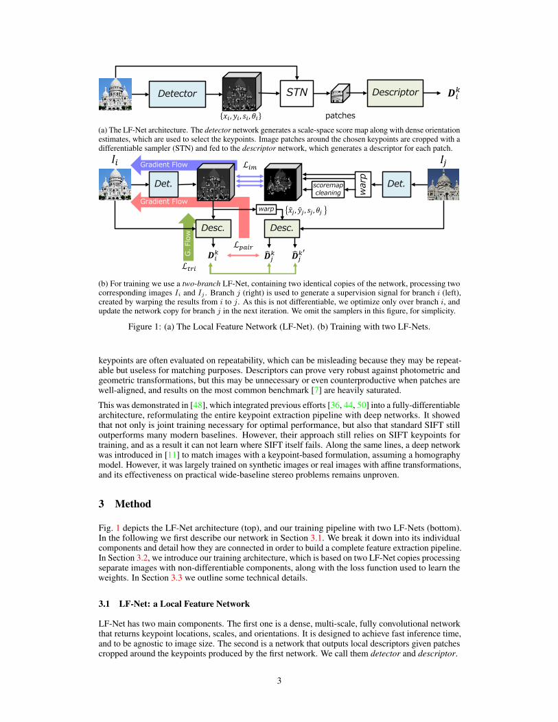
Detector STN
𝑥𝑥𝑖𝑖 ,𝑦𝑦𝑖𝑖 , 𝑠𝑠𝑖𝑖 ,𝜃𝜃𝑖𝑖
Descriptor 𝑫𝑫𝑖𝑖𝑘𝑘
patches(a) The LF-Net architecture. The detector network generates a scale-space score map along with dense orientationestimates, which are used to select the keypoints. Image patches around the chosen keypoints are cropped with adifferentiable sampler (STN) and fed to the descriptor network, which generates a descriptor for each patch.
Gradient Flow
Gradient Flow
Det. Det.
war
p
scoremapcleaning
ℒ𝑖𝑖𝑖𝑖
Desc. Desc.
warp
𝑫𝑫𝑖𝑖𝑘𝑘 �𝑫𝑫𝑗𝑗𝑘𝑘
ℒ𝑝𝑝𝑝𝑝𝑖𝑖𝑝𝑝�𝑫𝑫𝑗𝑗𝑘𝑘
′
ℒ𝑡𝑡𝑝𝑝𝑖𝑖
G. F
low
�𝑥𝑥𝑗𝑗 , �𝑦𝑦𝑗𝑗 , 𝑠𝑠𝑗𝑗 ,𝜃𝜃𝑗𝑗
𝐼𝐼𝑖𝑖 𝐼𝐼𝑗𝑗
(b) For training we use a two-branch LF-Net, containing two identical copies of the network, processing twocorresponding images Ii and Ij . Branch j (right) is used to generate a supervision signal for branch i (left),created by warping the results from i to j. As this is not differentiable, we optimize only over branch i, andupdate the network copy for branch j in the next iteration. We omit the samplers in this figure, for simplicity.
Figure 1: (a) The Local Feature Network (LF-Net). (b) Training with two LF-Nets.
keypoints are often evaluated on repeatability, which can be misleading because they may be repeat-able but useless for matching purposes. Descriptors can prove very robust against photometric andgeometric transformations, but this may be unnecessary or even counterproductive when patches arewell-aligned, and results on the most common benchmark [7] are heavily saturated.
This was demonstrated in [48], which integrated previous efforts [36, 44, 50] into a fully-differentiablearchitecture, reformulating the entire keypoint extraction pipeline with deep networks. It showedthat not only is joint training necessary for optimal performance, but also that standard SIFT stilloutperforms many modern baselines. However, their approach still relies on SIFT keypoints fortraining, and as a result it can not learn where SIFT itself fails. Along the same lines, a deep networkwas introduced in [11] to match images with a keypoint-based formulation, assuming a homographymodel. However, it was largely trained on synthetic images or real images with affine transformations,and its effectiveness on practical wide-baseline stereo problems remains unproven.
3 Method
Fig. 1 depicts the LF-Net architecture (top), and our training pipeline with two LF-Nets (bottom).In the following we first describe our network in Section 3.1. We break it down into its individualcomponents and detail how they are connected in order to build a complete feature extraction pipeline.In Section 3.2, we introduce our training architecture, which is based on two LF-Net copies processingseparate images with non-differentiable components, along with the loss function used to learn theweights. In Section 3.3 we outline some technical details.
3.1 LF-Net: a Local Feature Network
LF-Net has two main components. The first one is a dense, multi-scale, fully convolutional networkthat returns keypoint locations, scales, and orientations. It is designed to achieve fast inference time,and to be agnostic to image size. The second is a network that outputs local descriptors given patchescropped around the keypoints produced by the first network. We call them detector and descriptor.
3

In the remainder of this section, we assume that the images have been undistorted using the cameracalibration data. We convert them to grayscale for simplicity and simply normalize them individuallyusing their mean and standard deviation [42]. As will be discussed in Section 4.1, depth mapsand camera parameters can all be obtained using off-the-shelf SfM algorithms [34]. As depthmeasurements are often missing around 3D object boundaries—especially when computed SfMalgorithms—image regions for which we do not have depth measurements are masked and discardedduring training.
Feature map generation. We first use a fully convolutional network to generate a rich feature mapo from an image I, which can be used to extract keypoint locations as well as their attributes, i.e.,scale and orientation. We do this for two reasons. First, it has been shown that using such a mid-levelrepresentation to estimate multiple quantities helps increase the predictive power of deep nets [21].Second, it allows for larger batch sizes, that is, using more images simultaneously, which is key totraining a robust detector.
In practice, we use a simple ResNet [15] layout with three blocks. Each block contains 5 × 5convolutional filters followed by batch normalization [17], leaky-ReLU activations, and another setof 5× 5 convolutions. All convolutions are zero-padded to have the same output size as the input,and have 16 output channels. In our experiments, this has proved more successful that more recentarchitectures relying on strided convolutions and pixel shuffling [11].
Scale-invariant keypoint detection. To detect scale-invariant keypoints we propose a novel ap-proach to scale-space detection that relies on the feature map o. To generate a scale-space response,we resize it N times, at uniform intervals between 1/R and R, where N = 5 and R =
√2 in our
experiments. These are convolved with N independent 5× 5 filters size, which results in N scoremaps hn for 1 ≤ n < N , one for each scale. To increase the saliency of keypoints, we performa differentiable form of non-maximum suppression by applying a softmax operator over 15×15windows in a convolutional manner, which results in N sharper score maps, hn
1≤n<N . Since thenon-maximum suppression results are scale-dependent, we resize each hn back to the original imagesize, which yields hn
1≤n<N . Finally, we merge all the hn into a final scale-space score map, S, witha softmax-like operation. We define it as
S =∑n
hn � softmaxn(hn), (1)
where � is the Hadamard product.
From this scale-invariant map we choose the top K pixels as keypoints, and further apply a localsoftargmax [8] for sub-pixel accuracy. While selecting the the top K keypoints is not differentiable,this does not stop gradients from back-propagating through the selected points. Furthermore, thesub-pixel refinement through softargmax also makes it possible for gradients to flow through withrespect to keypoint coordinates.To predict the scale at each keypoint, we simply apply a softargmaxoperation over the scale dimension of hn. A simpler alternative would have been to directly regressthe scale once a keypoint has been detected. However, this turned out to be less effective in practice.
Orientation estimation. To learn orientations we follow the approach of [48, 50], but on the sharedfeature representation o instead of the image. We apply a single 5×5 convolution on o which outputstwo values for each pixel. They are taken to be the sine and cosine of the orientation and and used tocompute a dense orientation map θ using the arctan function.
Descriptor extraction. As discussed above, we extract from the score map S theK highest scoringfeature points and their image locations. With the scale map s and orientation map θ, this gives us Kquadruplets of the form pk = {x, y, s, θ}k, for which we want to compute descriptors.
To this end, we consider image patches around the selected keypoint locations. We crop them fromthe normalized images and resize them to 32× 32. To preserve differentiability, we use the bilinearsampling scheme of [18] for cropping. Our descriptor network comprises three 3× 3 convolutionalfilters with a stride of 2 and 64, 128, and 256 channels respectively. Each one is followed by batchnormalization and a ReLU activation. After the convolutional layers, we have a fully-connected512-channel layer, followed by batch normalization, ReLU, and a final fully-connected layer toreduce the dimensionality to M=256. The descriptors are l2 normalized and we denote them as D.
4

3.2 Learning LF-Net
As shown in Fig. 1, we formulate the learning problem in terms of a two-branch architecture whichtakes as input two images of the same scene, Ii and Ij , i 6= j, along with their respective depth mapsand the camera intrinsics and extrinsics, which can be obtained from conventional SfM methods.Given this data, we can warp the score maps to determine ground truth correspondences betweenimages. One distinctive characteristic of our setup is that branch j holds the components which breakdifferentiability, and is thus never back-propagated, in contrast to a traditional Siamese architecture.To do this in a mathematically sound way, we take inspiration from Q-learning [27] and use theparameters of the previous iteration of the network for this branch.
We formulate our training objective as a combination of two types of loss functions: image-level andpatch-level. Keypoint detection requires image-level operations and also affects where patches areextracted, thus we use both image-level and patch-level losses. For the descriptor network, we useonly patch-level losses as they operate independently for each patch once keypoints are selected.
Image-level loss. We can warp a score map with rigid-body transforms [12], using the projectivecamera model. We call this the SE(3) module w, which in addition to the score maps takes as inputthe camera pose P, calibration matrix K and depth map Z, for both images—note that we omit thelatter three for brevity. We propose to select K keypoints from the warped score map for Ij withstandard, non-differentiable non-maximum suppression, and generate a clean score map by placingGaussian kernels with standard deviation σ = 0.5 at those locations. We denote this operation g.Note that while it is non-differentiable, it only takes place on branch j, and thus has no effect in theoptimization. Mathematically, we write
Lim(Si,Sj) = |Si − g(w(Sj))|2 . (2)
Here, as mentioned before, occluded image regions are not used for optimization.
Patch-wise loss. With existing methods [3, 25, 36], the pool of pair-wise relationships is predefinedbefore training, assuming a detector is given. More importantly, forming these pairs from twodisconnected sets of keypoints will produce too many outliers for the training to ever converge.Finally, we want the gradients to flow back to the keypoint detector network, so that we are able tolearn keypoints that are good for matching.
We propose to solve this problem by leveraging the ground truth camera motion and depth to formsparse patch correspondences on the fly, by warping the detected keypoints. Note that we are onlyable to do this as we warp over branch j and back-propagate through branch i.
More specifically, once K keypoints are selected from Ii, we warp their spatial coordinates to Ij ,similarly as we do for the score maps to compute the image-level loss, but in the opposite direction.Note that we form the keypoint with scale and orientation from branch j, as they are not as sensitiveas the location, and we empirically found that it helps the optimization. We then extract descriptorsat these corresponding regions pk
i and pkj . If a keypoint falls on occluded regions after warping,
we drop it from the optimisation process. With these corresponding regions and their associateddecriptors Dk
i and Dkj we form Lpair which is used to train the detector network, i.e., the keypoint,
orientation, and scale components. Mathematically we write
Lpair(Dki , D
kj ) =
∑k
|Dki − Dk
j |2 . (3)
Similarly, in addition to the descriptors, we also enforce geometrical consistency over the orientationof the detected and warped points. We thus write
Lgeom(ski , θki , s
ki , θ
kj ) = λori
∑k
|θki − θkj |2 + λscale∑k
|ski − skj |2 , (4)
where s and θ respectively denotes the warped scale and orientation of a keypoint, by using therelative camera pose between the two images, and λori and λscale are weights.
Triplet loss for descriptors. To learn the descriptor, we also need to consider non-correspondingpairs of patches. Similar to [3], we form a triplet loss to learn the ideal embedding space for the
5

patches. However, for the positive pair we use the ground-truth geometry to find a match, as describedabove. For the negative—non-matching—pairs, we employ a progressive mining strategy to obtainthe most informative patches possible. Specifically, we sort the negatives for each sample by loss indecreasing order and sample randomly over the top M , where M = max(5, 64e
0.6k1000 ), where k is the
current iteration, i.e., we start with a pool of the 64 hardest samples and reduce it as the networksconverge, up to a minimum of 5. Sampling informative patches is critical to learn discriminativedescriptors, and random sampling will provide too many easy negative samples.
With the matching and non-matching pairs, we form the triplet loss as:
Ltri(Dki , D
kj , D
k′
j ) =∑k
max(0, |Dk
i − Dkj |2 − |Dk
i − Dk′
j |2 + C). (5)
where k′ 6= k, i.e., it can be any non-corresponding sample, and C=1 is the margin.
Loss function for each sub-network. In summary, the loss function that is used to learn eachsub-network is the following:• Detector loss: Ldet = Lim + λpairLpair + Lgeom
• Descriptor loss: Ldesc = Ltri
3.3 Technical details, otimization, and inference
To make the optimization more stable, we flip the images on each branch and merge the gradientsbefore updating. We emphasize here that with our loss, the gradients for the patch-wise loss cansafely back-propagate through branch i, including the top K selection, to the image-level networks.Likewise, the softargmax operator used for keypoint extraction allows the optimization to differentiatethe patch-wise loss with respect to the location of the keypoints.
Note that for inference we keep a single copy of the network, i.e., the architecture of Fig. 1-(a), andsimply run the differentiable part of the framework, branch i. Although differentiability is no longera concern, we still rely, for simplicity, on the spatial SoftMax for non-maximum supression and thesoftargmax and spatial transformers for patch sampling. Even so, our implementation can extract 512keypoints from QVGA frames (320×240) at 62 fps and from VGA frames (640×480) at 25 fps (42and 20 respectively for 1024 keypoints), on a Titan X PASCAL. Please refer to the supplementarymaterial for a thorough comparison of computational costs.
While training we extract 512 keypoints, as larger numbers become problematic due to memoryconstraints. This also allows us to maintain a batch with multiple image pairs (6), which helpsconvergence. Note that at test time we can choose as many keypoints as desired. As datasetswith natural images are composed of mostly upright images and are thus rather biased in terms oforientation, we perform data augmentation by randomly rotating the input patches by ±180o, andtransform the camera’s roll angle accordingly. We also perform scale augmentation by resizing theinput patches by 1/
√2 to√2, and transforming the focal length accordingly. This allows us to
train models comparable to traditional keypoint extraction pipelines, i.e., with built-in invariance torotation and scaling. However, in practice, many of the images in our indoors and outdoors examplesare upright, and the best-performing models are obtained by disabling these augmentations as wellas the orientation ans scale estimation completely. This is the approach followed by learned SLAMfront-ends such as [11]. We consider both strategies in the next section.
For optimization, we use ADAM [20] with a learning rate of 10−3. To balance the loss function forthe detector network we use λpair = 0.01, and λori = λscale = 0.1. Our implementation is writtenin TensorFlow and is publicly available.1
4 Experiments
4.1 Datasets
We consider both indoors and outdoors images as their characteristics drastically differ, as shownin Fig. 2. For indoors data we rely on ScanNet [10], an RGB-D dataset with over 2.5M images,
1https://github.com/vcg-uvic/lf-net-release
6

Figure 2: Samples from our indoors and outdoors datasets. Image regions without depth measure-ments, due to occlusions or sensor shortcomings, are drawn in red, and are simply excluded from theoptimization. Note the remaining artefacts in the depth maps for outdoors images.
including accurate camera poses from SfM reconstructions. These sequences show office settingswith specularities and very significant blurring artefacts, and the depth maps are incomplete due tosensing failures, specially around 3D object boundaries. The dataset provides training, validation,and test splits that we use accordingly. As this dataset is very large, we only use roughly half of theavailable sequences for training and validation, but test on the entire set of 312 sequences, pre-selectedby the authors, with the exception of LIFT. For LIFT we use a random subset of 43 sequences as theauthors’ implementation is too slow. To prevent selecting pairs of images that do not share any fieldof view, we sample images 15 frames away, guaranteeing enough scene overlap. At test time, weconsider multiple values for the frame difference to evaluate increasing baselines.
For outdoors data we use 25 photo-tourism image collections of popular landmarks collected by [16,39]. We run COLMAP [34] to obtain dense 3D reconstructions, including dense but noisy andinaccurate depth maps for every image. We post-process the depth maps by projecting each imagepixel to 3D space at the estimated depth, and mark it as invalid if the closest 3D point from thereconstruction is further than a threshold. The resulting depth maps are still noisy, but many occludedpixels are filtered out as shown in Fig. 2. To guarantee a reasonable degree of overlap for eachimage pair we perform a visibility check using the SfM points visible over both images. We considerbounding boxes twice the size of those containing these points to extract image regions roughlycorresponding, while ignoring very small ones. We use 14 sequences for training and validation,spliting the images into training and validation subsets by with a 70:30 ratio, and sample up to 50kpairs from each different scene. For testing we use the remaining 11 sequences, which were notused for training or validation, and sample up to 1k pairs from each set. We use square patches size256× 256 for training, for either data type.
4.2 Baselines and metrics
We consider the following full local feature pipelines: SIFT [23], SURF [6] ORB [32], A-KAZE [2],LIFT [48], and SuperPoint [11], using the authors’ release for the learned variants, LIFT and Super-Point, and OpenCV for the rest. For ScanNet, we test on 320×240 images, which is commensuratewith the patches cropped while training. We do the same for the baselines, as their performanceseems to be better than at higher resolutions, probably due to the low-texture nature of the images.For the outdoors dataset, we resize the images so that the largest dimensions is 640 pixels, as they arericher in texture, and all methods work better at this resolution. Similarly, we extract 1024 keypointsfor outdoors images, but limit them to 512 for Scannet, as the latter contains very little texture.
To evaluate the entire local feature pipeline performance, we use the matching score [24], whichis defined as the ratio of estimated correspondences that are correct according to the ground-truthgeometry, after obtaining them through nearest neighbour matching with the descriptors. As ourdata exhibits complex geometry, and to emphasize accurate localization of keypoints, similar to [31]we use a 5-pixel threshold instead of the overlap measure used in [24]. For results under differentthresholds please refer to the supplementary material.
4.3 Results on outdoors data
For this experiment we provide results independently for each sequence, in addition to the average.Due to the nature of the data, results vary from sequence to sequence. We provide quantitative results
7
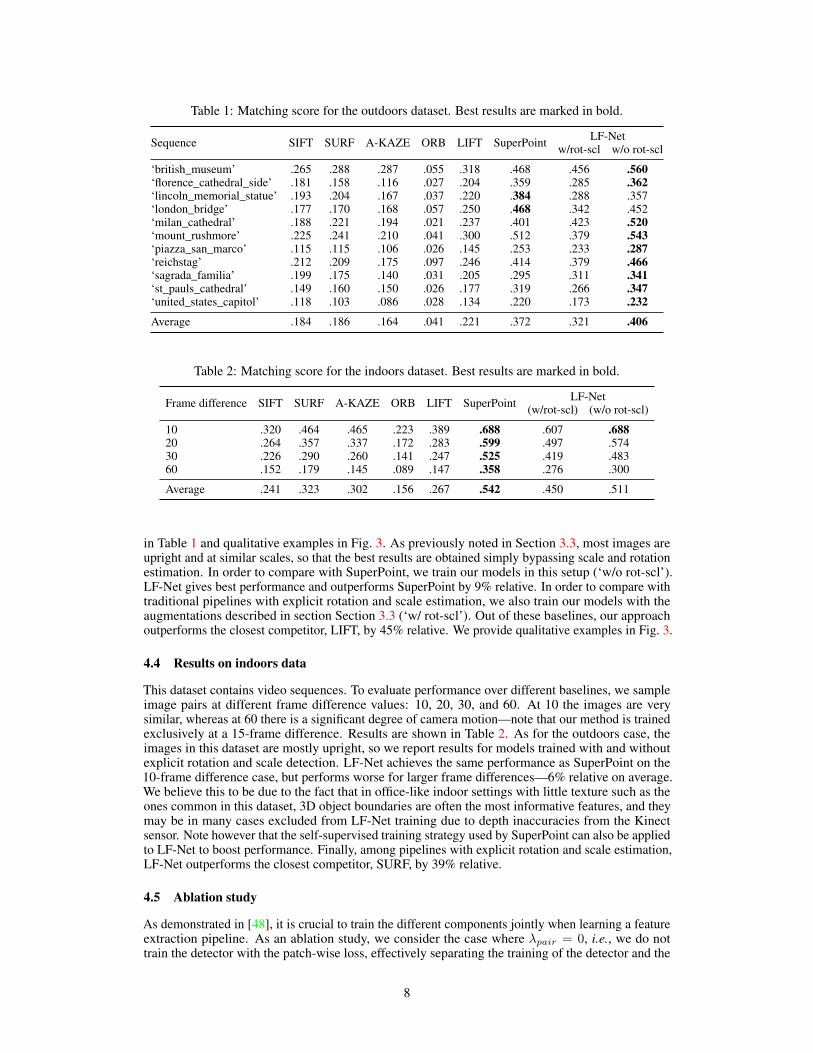
Table 1: Matching score for the outdoors dataset. Best results are marked in bold.
Sequence SIFT SURF A-KAZE ORB LIFT SuperPoint LF-Netw/rot-scl w/o rot-scl
‘british_museum’ .265 .288 .287 .055 .318 .468 .456 .560‘florence_cathedral_side’ .181 .158 .116 .027 .204 .359 .285 .362‘lincoln_memorial_statue’ .193 .204 .167 .037 .220 .384 .288 .357‘london_bridge’ .177 .170 .168 .057 .250 .468 .342 .452‘milan_cathedral’ .188 .221 .194 .021 .237 .401 .423 .520‘mount_rushmore’ .225 .241 .210 .041 .300 .512 .379 .543‘piazza_san_marco’ .115 .115 .106 .026 .145 .253 .233 .287‘reichstag’ .212 .209 .175 .097 .246 .414 .379 .466‘sagrada_familia’ .199 .175 .140 .031 .205 .295 .311 .341‘st_pauls_cathedral’ .149 .160 .150 .026 .177 .319 .266 .347‘united_states_capitol’ .118 .103 .086 .028 .134 .220 .173 .232
Average .184 .186 .164 .041 .221 .372 .321 .406
Table 2: Matching score for the indoors dataset. Best results are marked in bold.
Frame difference SIFT SURF A-KAZE ORB LIFT SuperPoint LF-Net(w/rot-scl) (w/o rot-scl)
10 .320 .464 .465 .223 .389 .688 .607 .68820 .264 .357 .337 .172 .283 .599 .497 .57430 .226 .290 .260 .141 .247 .525 .419 .48360 .152 .179 .145 .089 .147 .358 .276 .300
Average .241 .323 .302 .156 .267 .542 .450 .511
in Table 1 and qualitative examples in Fig. 3. As previously noted in Section 3.3, most images areupright and at similar scales, so that the best results are obtained simply bypassing scale and rotationestimation. In order to compare with SuperPoint, we train our models in this setup (‘w/o rot-scl’).LF-Net gives best performance and outperforms SuperPoint by 9% relative. In order to compare withtraditional pipelines with explicit rotation and scale estimation, we also train our models with theaugmentations described in section Section 3.3 (‘w/ rot-scl’). Out of these baselines, our approachoutperforms the closest competitor, LIFT, by 45% relative. We provide qualitative examples in Fig. 3.
4.4 Results on indoors data
This dataset contains video sequences. To evaluate performance over different baselines, we sampleimage pairs at different frame difference values: 10, 20, 30, and 60. At 10 the images are verysimilar, whereas at 60 there is a significant degree of camera motion—note that our method is trainedexclusively at a 15-frame difference. Results are shown in Table 2. As for the outdoors case, theimages in this dataset are mostly upright, so we report results for models trained with and withoutexplicit rotation and scale detection. LF-Net achieves the same performance as SuperPoint on the10-frame difference case, but performs worse for larger frame differences—6% relative on average.We believe this to be due to the fact that in office-like indoor settings with little texture such as theones common in this dataset, 3D object boundaries are often the most informative features, and theymay be in many cases excluded from LF-Net training due to depth inaccuracies from the Kinectsensor. Note however that the self-supervised training strategy used by SuperPoint can also be appliedto LF-Net to boost performance. Finally, among pipelines with explicit rotation and scale estimation,LF-Net outperforms the closest competitor, SURF, by 39% relative.
4.5 Ablation study
As demonstrated in [48], it is crucial to train the different components jointly when learning a featureextraction pipeline. As an ablation study, we consider the case where λpair = 0, i.e., we do nottrain the detector with the patch-wise loss, effectively separating the training of the detector and the
8
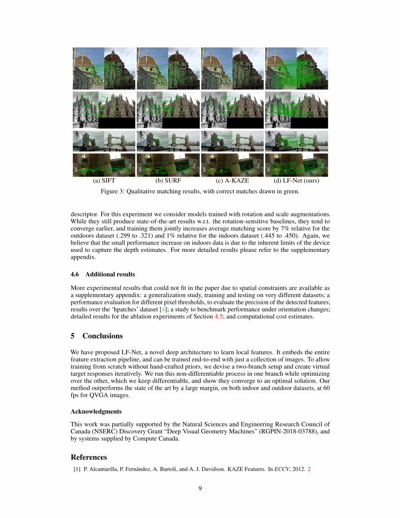
(a) SIFT (b) SURF (c) A-KAZE (d) LF-Net (ours)
Figure 3: Qualitative matching results, with correct matches drawn in green.
descriptor. For this experiment we consider models trained with rotation and scale augmentations.While they still produce state-of-the-art results w.r.t. the rotation-sensitive baselines, they tend toconverge earlier, and training them jointly increases average matching score by 7% relative for theoutdoors dataset (.299 to .321) and 1% relative for the indoors dataset (.445 to .450). Again, webelieve that the small performance increase on indoors data is due to the inherent limits of the deviceused to capture the depth estimates. For more detailed results please refer to the supplementaryappendix.
4.6 Additional results
More experimental results that could not fit in the paper due to spatial constraints are available asa supplementary appendix: a generalization study, training and testing on very different datasets; aperformance evaluation for different pixel thresholds, to evaluate the precision of the detected features;results over the ‘hpatches’ dataset [4]; a study to benchmark performance under orientation changes;detailed results for the ablation experiments of Section 4.5; and computational cost estimates.
5 Conclusions
We have proposed LF-Net, a novel deep architecture to learn local features. It embeds the entirefeature extraction pipeline, and can be trained end-to-end with just a collection of images. To allowtraining from scratch without hand-crafted priors, we devise a two-branch setup and create virtualtarget responses iteratively. We run this non-differentiable process in one branch while optimizingover the other, which we keep differentiable, and show they converge to an optimal solution. Ourmethod outperforms the state of the art by a large margin, on both indoor and outdoor datasets, at 60fps for QVGA images.
Acknowledgments
This work was partially supported by the Natural Sciences and Engineering Research Council ofCanada (NSERC) Discovery Grant “Deep Visual Geometry Machines” (RGPIN-2018-03788), andby systems supplied by Compute Canada.
References[1] P. Alcantarilla, P. Fernández, A. Bartoli, and A. J. Davidson. KAZE Features. In ECCV, 2012. 2
9

[2] P. F. Alcantarilla, J. Nuevo, and A. Bartoli. Fast Explicit Diffusion for Accelerated Features in NonlinearScale Spaces. In BMVC, 2013. 7
[3] V. Balntas, E. Johns, L. Tang, and K. Mikolajczyk. PN-Net: Conjoined Triple Deep Network for LearningLocal Image Descriptors. In arXiv Preprint, 2016. 2, 5
[4] V. Balntas, K. Lenc, A. Vedaldi, and K. Mikolajczyk. Hpatches: A benchmark and evaluation of handcraftedand learned local descriptors. In CVPR, 2017. 9, 13
[5] H. Bay, A. Ess, T. Tuytelaars, and L. Van Gool. SURF: Speeded Up Robust Features. CVIU, 10(3):346–359,2008. 2
[6] H. Bay, T. Tuytelaars, and L. Van Gool. SURF: Speeded Up Robust Features. In ECCV, 2006. 7[7] M. Brown, G. Hua, and S. Winder. Discriminative Learning of Local Image Descriptors. PAMI, 2011. 3[8] O. Chapelle and M. Wu. Gradient Descent Optimization of Smoothed Information Retrieval Metrics.
Information Retrieval, 13(3):216–235, 2009. 4[9] C. Choy, J. Gwak, S. Savarese, and M. Chandraker. Universe Correspondence Network. In NIPS, 2016. 1,
2[10] A. Dai, A. Chang, M. Savva, M. Halber, T. Funkhouser, and M. Nießner. Scannet: Richly-Annotated 3D
Reconstructions of Indoor Scenes. In CVPR, 2017. 6[11] D. Detone, T. Malisiewicz, and A. Rabinovich. Superpoint: Self-Supervised Interest Point Detection and
Description. CVPR Workshop on Deep Learning for Visual SLAM, 2018. 1, 3, 4, 6, 7[12] J. Engel, T. Schöps, and D. Cremers. LSD-SLAM: Large-Scale Direct Monocular SLAM. In ECCV, 2014.
5[13] X. Han, T. Leung, Y. Jia, R. Sukthankar, and A. C. Berg. MatchNet: Unifying Feature and Metric Learning
for Patch-Based Matching. In CVPR, 2015. 2[14] R. Hartley and A. Zisserman. Multiple View Geometry in Computer Vision. Cambridge University Press,
2000. 2[15] K. He, X. Zhang, S. Ren, and J. Sun. Deep Residual Learning for Image Recognition. In CVPR, pages
770–778, 2016. 4[16] J. Heinly, J. Schoenberger, E. Dunn, and J.-M. Frahm. Reconstructing the World in Six Days. In CVPR,
2015. 7[17] S. Ioffe and C. Szegedy. Batch Normalization: Accelerating Deep Network Training by Reducing Internal
Covariate Shift. In ICML, 2015. 4[18] M. Jaderberg, K. Simonyan, A. Zisserman, and K. Kavukcuoglu. Spatial Transformer Networks. In NIPS,
pages 2017–2025, 2015. 4[19] M. Keller, Z. Chen, F. Maffra, P. Schmuck, and M. Chli. Learning Deep Descriptors with Scale-Aware
Triplet Networks. In CVPR, 2018. 2[20] D. Kingma and J. Ba. Adam: A Method for Stochastic Optimisation. In ICLR, 2015. 6[21] I. Kokkinos. Ubernet: Training a Universal Convolutional Neural Network for Low-, Mid-, and High-Level
Vision Using Diverse Datasets and Limited Memory. In CVPR, 2017. 4[22] K. Lenc and A. Vedaldi. Learning Covariant Feature Detectors. In ECCV, 2016. 2[23] D. Lowe. Distinctive Image Features from Scale-Invariant Keypoints. IJCV, 20(2), 2004. 1, 2, 7[24] K. Mikolajczyk and C. Schmid. A Performance Evaluation of Local Descriptors. PAMI, 27(10):1615–1630,
2004. 7[25] A. Mishchuk, D. Mishkin, F. Radenovic, and J. Matas. Working Hard to Know Your Neighbor’s Margins:
Local Descriptor Learning Loss. In NIPS, 2017. 2, 5[26] D. Mishkin, F. Radenovic, and J. Matas. Repeatability Is Not Enough: Learning Affine Regions via
Discriminability. In ECCV, 2018. 2[27] V. Mnih, K. Kavukcuoglu, D. Silver, A. Rusu, J. Veness, M. Bellemare, A. Graves, M. Riedmiller,
A. Fidjeland, G. Ostrovski, S. Petersen, C. Beattie, A. Sadik, I. Antonoglou, H. King, D. Kumaran,D. Wierstra, S. Legg, and D. Hassabis. Human-Level Control through Deep Reinforcement Learning.Nature, 518(7540):529–533, February 2015. 5
[28] D. Mukherjee, Q. M. J. Wu, and G. Wang. A Comparative Experimental Study of Image Feature Detectorsand Descriptors. MVA, 26(4):443–466, 2015. 2
[29] R. Mur-artal, J. Montiel, and J. Tardós. Orb-Slam: A Versatile and Accurate Monocular Slam System.IEEE Transactions on Robotics, 31(5):1147–1163, 2015. 2
[30] E. Rosten and T. Drummond. Machine Learning for High-Speed Corner Detection. In ECCV, 2006. 2[31] E. Rosten, R. Porter, and T. Drummond. Faster and Better: A Machine Learning Approach to Corner
Detection. PAMI, 32:105–119, 2010. 2, 7[32] E. Rublee, V. Rabaud, K. Konolidge, and G. Bradski. ORB: An Efficient Alternative to SIFT or SURF. In
ICCV, 2011. 2, 7[33] N. Savinov, A. Seki, L. Ladicky, T. Sattler, and M. Pollefeys. Quad-Networks: Unsupervised Learning to
Rank for Interest Point Detection. CVPR, 2017. 1, 2[34] J. Schönberger and J. Frahm. Structure-From-Motion Revisited. In CVPR, 2016. 1, 4, 7[35] J. Schönberger, H. Hardmeier, T. Sattler, and M. Pollefeys. Comparative Evaluation of Hand-Crafted and
Learned Local Features. In CVPR, 2017. 2[36] E. Simo-serra, E. Trulls, L. Ferraz, I. Kokkinos, P. Fua, and F. moreno-noguer. Discriminative Learning of
Deep Convolutional Feature Point Descriptors. In ICCV, 2015. 2, 3, 5[37] K. Simonyan, A. Vedaldi, and A. Zisserman. Learning Local Feature Descriptors Using Convex Optimisa-
tion. PAMI, 2014. 2
10

[38] C. Strecha, A. Bronstein, M. Bronstein, and P. Fua. LDAHash: Improved Matching with SmallerDescriptors. PAMI, 34(1), January 2012. 2
[39] B. Thomee, D. Shamma, G. Friedland, B. Elizalde, K. Ni, D. Poland, D. Borth, and L. Li. YFCC100M:the New Data in Multimedia Research. In CACM, 2016. 7
[40] Y. Tian, B. Fan, and F. Wu. L2-Net: Deep Learning of Discriminative Patch Descriptor in Euclidean Space.In CVPR, 2017. 2
[41] E. Tola, V. Lepetit, and P. Fua. Daisy: An Efficient Dense Descriptor Applied to Wide Baseline Stereo.PAMI, 32(5):815–830, 2010. 2
[42] D. Ulyanov, A. Vedaldi, and V. Lempitsky. Improved Texture Networks: Maximizing Quality and Diversityin Feed-Forward Stylization and Texture Synthesis. In CVPR, 2017. 4
[43] B. Ummenhofer, H. Zhou, J. Uhrig, N. Mayer, E. Ilg, A. Dosovitskiy, and T. Brox. Demon: Depth andMotion Network for Learning Monocular Stereo. In CVPR, 2017. 1, 2
[44] Y. Verdie, K. M. Yi, P. Fua, and V. Lepetit. TILDE: A Temporally Invariant Learned DEtector. In CVPR,2015. 2, 3
[45] S. Vijayanarasimhan, S. Ricco, C. Schmid, R. Sukthankar, and K. Fragkiadaki. Sfm-Net: Learning ofStructure and Motion from Video. arXiv Preprint, 2017. 1, 2
[46] X. Wei, Y. Zhang, Y. Gong, and N. Zheng. Kernelized Subspace Pooling for Deep Local Descriptors. InCVPR, 2018. 2
[47] C. Wu. Towards Linear-Time Incremental Structure from Motion. In 3DV, 2013. 2[48] K. M. Yi, E. Trulls, V. Lepetit, and P. Fua. LIFT: Learned Invariant Feature Transform. In ECCV, 2016. 1,
2, 3, 4, 7, 8[49] K. M. Yi, E. Trulls, Y. Ono, V. Lepetit, M. Salzmann, and P. Fua. Learning to Find Good Correspondences.
In CVPR, 2018. 1[50] K. M. Yi, Y. Verdie, P. Fua, and V. Lepetit. Learning to Assign Orientations to Feature Points. In CVPR,
2016. 2, 3, 4[51] S. Zagoruyko and N. Komodakis. Learning to Compare Image Patches via Convolutional Neural Networks.
In CVPR, 2015. 2[52] A. R. Zamir, T. Wekel, P. Agrawal, J. Malik, and S. Savarese. Generic 3D Representation via Pose
Estimation and Matching. In ECCV, 2016. 1, 2[53] T. Zhou, M. Brown, N. Snavely, and D. Lowe. Unsupervised Learning of Depth and Ego-Motion from
Video. In CVPR, 2017. 1, 2
11

6 Appendix
6.1 Generalization performance
We test the models trained on indoors data with outdoors data, and vice-versa, to benchmark theirgeneralization performance, determining how well they perform on images with very differentgeometric and photometric properties than seen while training. For this experiment we use modelstrained with rotation and scale augmentations. The performance drop training with outdoors dataand testing with indoors data is 18% relative (.450 to .370 matching score). The performance droptraining with indoors data and testing with outdoors data is 8% relative (.321 to .295 in matchingscore). Compared to the rotation-sensitive baselines, the performance still remains state-of-the-art, bya large margin.
6.2 Computational cost
As outlined in Section 3.3, LF-Net can extract 512 keypoints from QVGA frames (320×240) at 62 fpsand from VGA frames (640×480) at 25 fps (42 and 20 respectively for 1024 keypoints), on a Titan XPASCAL. Table 3 lists the computational cost for different keypoint extraction pipelines. As theyare designed to operate in different regimes, we normalize the timings by the number of keypointsgenerated by each method, and provide the mean cost of extracting a single keypoint in micro-seconds.For SuperPoint we use the available implementation, which has some computational overhead due toimage loading and pre-processing—the authors claim a runtime of 70 fps at VGA resolutions, whichshould be achievable. LIFT’s modular implementation is provided only for reference, and should behighly optimizable at inference time.
Table 3: Computational cost for different keypoint extraction pipelines. The estimates are normalizedby the number of keypoints and given in micro-seconds. *) For SuperPoint, running on smaller imagesize gives less keypoints, and therefore the increase in per-keypoint computation time.
Input size 320 × 240 640 × 480
LF-Net (512 kp) 31.5 78.1LF-Net (1024 kp) 23.2 48.8SIFT 62.7 55.9SURF 10.0 10.0A-KAZE 39.1 25.1ORB 17.6 49.3LIFT 509 · 103 119 · 103SuperPoint 263.7∗ 130.9∗
6.3 Geometric precision
In the paper we consider only a threshold of 5 pixels to determine correct matches, which doesnot necessarily capture how accurate each keypoint is. To overcome the limitation of this setup, inTables 4 and 5 we report matching score results for different pixel thresholds, from 1 to 5. Our methodoutperforms SIFT and SURF at any threshold other than sub-pixel, and can double their performanceat higher thresholds for certain datasets. Note that sub-pixel results are not fully trustworthy, as thedepth estimates are quite noisy, and our method would benefit from better training and test data.
Table 4: Matching score: Outdoors
Threshold (pix) 1 2 3 4 5
SIFT .111 .162 .175 .180 .184SURF .068 .130 .160 .176 .186LF-Net .102 .229 .284 .308 .321
12

Table 5: Matching score: Indoors. Please note that these results were obtained over a subset of thedata used in Section 4.4, which explains the small difference with Table 2.
Threshold (pix) 1 2 3 4 5
SIFT .072 .151 .196 .223 .241SURF .074 .170 .240 .288 .323LF-Net .066 .189 .298 .383 .450
6.4 Results on the ‘hpatches’ dataset
In Table 6 we report matching score results for the ‘hpatches’ dataset [4]. As in the previous section,we consider multiple pixel thresholds. As before, LF-Net outperforms classical algorithms except atthe sub-pixel level.
Table 6: Matching score: Outdoors
Feature Sequence Pixel threshold1 2 3 4 5
SIFTViewpoint
.206 .290 .324 .310 .319SURF .138 .258 .312 .337 .351LF-Net .131 .265 .311 .329 .339
SIFTIllumination
.180 .248 .267 .274 .279SURF .162 .245 .309 .281 .298LF-Net .171 .310 .360 .378 .389
SIFTAverage
.193 .269 .288 .296 .301SURF .150 .252 .296 .317 .330LF-Net .151 .288 .335 .354 .364
6.5 Rotation invariance
To measure the rotation invariance of each keypoint type, we match a subset of the outdoors datasets,500 image pairs from different sequences, while applying in-plane rotations to the images every 10o,from 0 to 360o, and average the matching score over each bin. The results are listed in Table 7. Asexpected, the models learned without rotation invariance may excel when the images are well aligned(Table 1) but perform very poorly overall.
Table 7: Average matching score under rotationsFeature Avg. matching score
SIFT .265SURF .208LF-Net (w/ rot-scl) .338SuperPoint .092LF-Net (w/o rot-scl) .074
13