liaison user manual - isp. · pdf filemonospace $schrodinger/maestro file names, directory...
TRANSCRIPT

Liaison User Manual
Liaison 5.5
User Manual
Schrödinger Press

Liaison User Manual Copyright © 2009 Schrödinger, LLC. All rights reserved.
While care has been taken in the preparation of this publication, Schrödinger
assumes no responsibility for errors or omissions, or for damages resulting from
the use of the information contained herein.
Canvas, CombiGlide, ConfGen, Epik, Glide, Impact, Jaguar, Liaison, LigPrep,
Maestro, Phase, Prime, PrimeX, QikProp, QikFit, QikSim, QSite, SiteMap, Strike, and
WaterMap are trademarks of Schrödinger, LLC. Schrödinger and MacroModel are
registered trademarks of Schrödinger, LLC. MCPRO is a trademark of William L.
Jorgensen. Desmond is a trademark of D. E. Shaw Research. Desmond is used with
the permission of D. E. Shaw Research. All rights reserved. This publication may
contain the trademarks of other companies.
Schrödinger software includes software and libraries provided by third parties. For
details of the copyrights, and terms and conditions associated with such included
third party software, see the Legal Notices for Third-Party Software in your product
installation at $SCHRODINGER/docs/html/third_party_legal.html (Linux OS) or
%SCHRODINGER%\docs\html\third_party_legal.html (Windows OS).
This publication may refer to other third party software not included in or with
Schrödinger software ("such other third party software"), and provide links to third
party Web sites ("linked sites"). References to such other third party software or
linked sites do not constitute an endorsement by Schrödinger, LLC. Use of such
other third party software and linked sites may be subject to third party license
agreements and fees. Schrödinger, LLC and its affiliates have no responsibility or
liability, directly or indirectly, for such other third party software and linked sites,
or for damage resulting from the use thereof. Any warranties that we make
regarding Schrödinger products and services do not apply to such other third party
software or linked sites, or to the interaction between, or interoperability of,
Schrödinger products and services and such other third party software.
June 2009

Contents
Document Conventions ...................................................................................................... v
Chapter 1: Introduction ....................................................................................................... 1
1.1 About Liaison............................................................................................................. 1
1.2 Liaison Binding Energy Models.............................................................................. 2
1.2.1 LIA Model Equation............................................................................................. 2
1.2.2 LiaisonScore Model Equation ............................................................................. 3
1.3 Running Schrödinger Software .............................................................................. 3
1.4 Citing Liaison in Publications ................................................................................. 3
Chapter 2: Liaison Tutorial ............................................................................................... 5
2.1 Preparation ................................................................................................................. 5
2.2 Starting Maestro ....................................................................................................... 6
2.3 Running the Liaison Simulations ........................................................................... 6
2.3.1 Setting Up the System ........................................................................................ 7
2.3.2 Starting and Monitoring the Liaison Job ............................................................. 8
2.4 Generating and Validating an LIA Model of Binding Affinity ............................ 9
2.4.1 Importing Liaison Results into Strike for Model Creation .................................... 9
2.4.2 Selecting Training Set Molecules ...................................................................... 11
2.4.3 Creating the LIA Model to Predict Binding Affinities ......................................... 11
2.4.4 Analyzing the LIA Binding Affinity Model .......................................................... 13
2.4.5 Predicting Binding Affinities with the LIA Model................................................ 13
2.4.6 Analyze LIA Binding Affinity Predictions for the Test Set .................................. 15
2.4.7 Making Predictions for Additional Molecules..................................................... 16
2.5 Generating and Applying LiaScore and ELR Binding Affinity Models.......... 16
Chapter 3: Protein and Ligand Preparation........................................................ 19
3.1 Protein Preparation ................................................................................................. 19
3.2 Checking the Protein Structures .......................................................................... 21
3.2.1 Checking the Orientation of Water Molecules................................................... 22
Liaison 5.5 User Manual iii

Contents
iv
3.2.2 Checking for Steric Clashes.............................................................................. 22
3.2.3 Resolving H-Bonding Conflicts ......................................................................... 22
3.3 Ligand Preparation ................................................................................................. 23
3.3.1 Using LigPrep for Ligand Preparation ............................................................... 24
3.3.2 Using Other Programs for Ligand Preparation.................................................. 26
Chapter 4: Running Liaison........................................................................................... 27
4.1 Overview of Liaison Tasks..................................................................................... 27
4.2 The Liaison Panel .................................................................................................... 29
4.2.1 Systems Tab ..................................................................................................... 29
4.2.2 Parameters Tab................................................................................................. 30
4.2.3 Analysis Tab...................................................................................................... 32
4.3 Running Liaison From the Command Line ........................................................ 33
Chapter 5: Technical Notes for Liaison.................................................................. 35
5.1 Models of Ligand Binding...................................................................................... 35
5.1.1 Limitations of Free-Energy Perturbation ........................................................... 36
5.1.2 Advantages of Linear Response Methods ........................................................ 36
5.1.3 Advantages of Liaison....................................................................................... 37
5.2 LiaisonScore Binding Free Energy Model .......................................................... 38
5.3 Application to HIV Reverse Transcriptase .......................................................... 39
5.4 Application to ß-Secretase (BACE) Inhibitors.................................................... 43
Getting Help ............................................................................................................................. 45
Index .............................................................................................................................................. 49
Liaison 5.5 User Manual

Document Conventions
In addition to the use of italics for names of documents, the font conventions that are used inthis document are summarized in the table below.
Links to other locations in the current document or to other PDF documents are colored likethis: Document Conventions.
In descriptions of command syntax, the following UNIX conventions are used: braces { }
enclose a choice of required items, square brackets [ ] enclose optional items, and the barsymbol | separates items in a list from which one item must be chosen. Lines of commandsyntax that wrap should be interpreted as a single command.
File name, path, and environment variable syntax is generally given with the UNIX conven-tions. To obtain the Windows conventions, replace the forward slash / with the backslash \ inpath or directory names, and replace the $ at the beginning of an environment variable with a% at each end. For example, $SCHRODINGER/maestro becomes %SCHRODINGER%\maestro.
In this document, to type text means to type the required text in the specified location, and toenter text means to type the required text, then press the ENTER key.
References to literature sources are given in square brackets, like this: [10].
Font Example Use
Sans serif Project Table Names of GUI features, such as panels, menus,menu items, buttons, and labels
Monospace $SCHRODINGER/maestro File names, directory names, commands, envi-ronment variables, and screen output
Italic filename Text that the user must replace with a value
Sans serifuppercase
CTRL+H Keyboard keys
Liaison 5.5 User Manual v

vi
Liaison 5.5 User Manual
Liaison User Manual
Chapter 1
Chapter 1: Introduction
1.1 About Liaison
Liaison predicts ligand-receptor binding affinities using a linear interaction approximation(LIA) model that has been fitted to a set of known binding free energies. For each ligand in thetraining set, Liaison runs molecular mechanics (MM) simulations of the ligand-receptorcomplex at both endpoints of the binding process, bound ligand and free ligand. The simula-tion data and empirical binding affinities are analyzed to generate the Liaison parameters: α, β,and γ. These parameters are subsequently used to predict binding energies for other ligandswith the same receptor. Liaison simulations use a continuum solvation model to shortensampling times and speed convergence.
Liaison is run primarily from the Maestro graphical user interface. A tutorial in using Liaisonfrom Maestro appears in Chapter 2. Liaison can also be run from the command line, asdescribed in Chapter 5. Utilities and scripts are run from the command line. Liaison technicalnotes, background, and references are provided in Chapter 5.
Maestro is Schrödinger’s powerful, unified, multi-platform graphical user interface (GUI). Itis designed to simplify modeling tasks, such as molecule building and data analysis, and also tofacilitate the set up and submission of jobs to Schrödinger’s computational programs. Themain Maestro features include a project-based data management facility, a scripting languagefor automating large or repetitive tasks, a wide range of useful display options, a comprehen-sive molecular builder, and surfacing and entry plotting facilities. For detailed informationabout the Maestro interface, see the Maestro online help or the Maestro User Manual.
Protein Preparation is strongly recommended for protein and protein-ligand complex PDBstructures to be used in Liaison. In most cases, this can be performed in Maestro, using theProtein Preparation Wizard panel on the Workflows menu. Protein and ligand preparation aredescribed in Chapter 3.
The Impact computational program runs the MM calculations for Liaison simulations, whichcan be carried out using molecular dynamics (MD), hybrid Monte Carlo (HMC), or energyminimization. Impact uses an OPLS-AA force field. Impact calculations can also be run inde-pendently of Liaison. For more information, see the Impact User Manual and the ImpactCommand Reference Manual.
The Strike statistical analysis package is used for the fitting and prediction analysis tasks ofLiaison. For more information, see the Strike User Manual.
Liaison 5.5 User Manual 1

Chapter 1: Introduction
2
1.2 Liaison Binding Energy Models
1.2.1 LIA Model Equation
A Liaison simulation combines a molecular-mechanics calculation with experimental data tobuild a model scoring function used to correlate or to predict ligand-protein binding free ener-gies. The assumption used is that the binding energy can be approximated by comparing theenergy of the bound complex with the energy of the free ligand-receptor system. A method ofthis type is called a Linear Response Method (LRM), a Linear Interaction Approximation(LIA), or a Linear Interaction Energy (LIE) method.
A novel feature of Liaison is that the simulation takes place in implicit (continuum) rather thanexplicit solvent—hence the name Liaison, for Linear Interaction Approximation in ImplicitSOlvatioN. The explicit-solvent version of the methodology was first suggested by Aqvist(Hansson, T.; Aqvist, J. Protein Eng. 1995, 8, 1137-1145), based on approximating thecharging integral in the free-energy-perturbation formula with a mean-value approach, inwhich the integral is represented as half the sum of the values at the endpoints, namely the freeand bound states of the ligand. The empirical relationship used by Liaison is shown below:
∆G = α (<Ubvdw> – <Uf
vdw >) + β (<Ubelec > – <Uf
elec>) + γ (<Ubcav> – <U f
cav>)
Here < > represents the ensemble average, b represents the bound form of the ligand, f repre-sents the free form of the ligand, and α, β, and γ are the coefficients. Uvdw, Uelec, and Ucav arethe van der Waals, electrostatic, and cavity energy terms in the Surface Generalized Born(SGB) continuum solvent model. The cavity energy term, Ucav, is proportional to the exposedsurface area of the ligand. Thus, the difference:
<Ub cav> – <U f
cav>
measures the surface area lost by contact with the receptor. The net electrostatic interaction-energy in continuum solvent is given by:
Uelec = Ucoul + 2 Urxnf
where Ucoul is the Coulomb interaction energy and Urxnf is the SGB-solvent reaction-fieldenergy. (The factor of 2 compensates for the division by 2 made in the definition of the reac-tion-field free energy.)
In most applications, the coefficients α, β, and γ are determined empirically by fitting to theexperimentally determined free energies of binding for a training set of ligands. In such appli-cations, Liaison’s simulation task is used to calculate the values of Uvdw, U elec, and U cav for thebound (complexed) and unbound (free) states of the training-set ligands, and its analysis task isused to derive values for the α, β, and γ fitting coefficients. The fitted equation can then be usedto predict the binding affinities of additional ligands. In the current version of Liaison, a
Liaison 5.5 User Manual

Chapter 1: Introduction
constant term is added to ∆G in the fitting process, and is adjusted during the fit. This corre-sponds to an extension of the strict linear response model.
1.2.2 LiaisonScore Model Equation
Liaison also calculates a scoring function similar to GlideScore over the course of the LRMsimulation. This scoring function, previously called “GlideScore in Liaison,” is called Liaison-Score in Liaison 5.5. The average LiaisonScore can then be used to predict binding energiesusing the alternate model:
∆G = a(<LiaisonScore>) + b
where a is the LiaisonScore coefficient and b is a constant.
1.3 Running Schrödinger Software
To run any Schrödinger program on a UNIX platform, or start a Schrödinger job on a remotehost from a UNIX platform, you must first set the SCHRODINGER environment variable to theinstallation directory for your Schrödinger software. To set this variable, enter the followingcommand at a shell prompt:
Once you have set the SCHRODINGER environment variable, you can start Maestro with thefollowing command:
$SCHRODINGER/maestro &
It is usually a good idea to change to the desired working directory before starting Maestro.This directory then becomes Maestro’s working directory. For more information on startingMaestro, including starting Maestro on a Windows platform, see Section 2.1 of the MaestroUser Manual.
1.4 Citing Liaison in Publications
The use of this product and its components should be acknowledged in publications as:
Liaison, version 5.5, Schrödinger, LLC, New York, NY, 2009; Strike, version 1.8, Schrödinger,LLC, New York, NY, 2009.
csh/tcsh: setenv SCHRODINGER installation-directory
bash/ksh: export SCHRODINGER=installation-directory
Liaison 5.5 User Manual 3

4
Liaison 5.5 User Manual
Liaison User Manual
Chapter 2
Chapter 2: Liaison Tutorial
This chapter contains tutorial exercises to help you quickly become familiar with the function-ality of Liaison using the Maestro interface. Liaison is used to simulate and predict bindingaffinities. It does so by generating for each protein-ligand complex the descriptors necessary toapply the LIA equation, the LiaScore, which is the GlideScore computed over discrete proteinatom locations rather than over a gridded protein representation, and the LiaScore componentswhich may be used to generate an ELR model. Models for the binding affinity are then createdand applied from Liaison-generated descriptors via Strike. Thus, the Liaison process involvestwo steps, the simulation of binding in Liaison to generate a set of descriptors and the creationand application of binding affinity models from the Liaison descriptors with Strike.
The exercises in this chapter demonstrate:
• How to perform Liaison simulations on multiple ligands
• How to create a validated model for the α, β, and γ coefficients for the LIA equationusing Strike
• How to generate and apply the results of Liaison simulations to predict binding affinitiesfor novel ligands
• How to create and apply LiaScore and Extended Linear Response (ELR) models to pre-dict binding affinities
You will use the Liaison panel to set up and run Liaison simulations and then use the Strikepanels to create, validate, and apply binding affinity models from Strike.
To do these exercises you must have access to an installed version of Maestro 9.0, Liaison 5.5and Strike 1.8. For installation instructions, see the Installation Guide.
2.1 Preparation
Before you start Maestro and begin the exercises, you must first create a local tutorial directorytree. Some exercises in this tutorial produce files that are needed in subsequent exercises. Toallow you to begin at any exercise you choose, the $SCHRODINGER/impact-vversion/tutorial/liaison directory contains copies of the relevant input and output files that willbe generated as you perform the tutorial.
Liaison 5.5 User Manual 5

Chapter 2: Liaison Tutorial
6
To create a local directory tree:
1. At a shell prompt, change to a directory in which you have write permissions.
2. Create a local base directory:
mkdir basedir
In the text, this directory is referred to as the base directory.
3. In the base directory, create a soft link to the $SCHRODINGER/impact-vversion/tutorial/liaison directory by entering the following command:
ln –s $SCHRODINGER/impact-vversion/tutorial/liaison .
2.2 Starting Maestro
You do not need to start Maestro until you begin an exercise. If you have not started Maestrobefore, this section contains instructions.
To start Maestro:
1. Set the SCHRODINGER environment variable to the directory in which Maestro and Liai-son are installed:
2. Change to the desired working directory.
cd basedir
3. Enter the command:
$SCHRODINGER/maestro &
You are now ready to proceed with the exercises below.
2.3 Running the Liaison Simulations
In this exercise, starting with a receptor and a set of prepared ligands, you will set up and run ajob that calculates Liaison descriptors. The descriptors are saved in a Maestro file and a CSVfile, allowing you to use them in the creation, validation, and application of LIA, LiaScore andELR models of binding affinity.
The Liaison calculations to be run in this exercise require about 1.5 hours of CPU time on asingle 2.8 GHz Xeon processor, though by taking advantage of multiple processors this time
csh/tcsh: setenv SCHRODINGER installation_path
sh/bash/ksh: export SCHRODINGER=installation_path
Liaison 5.5 User Manual

Chapter 2: Liaison Tutorial
can be reduced sharply. The output files from the Liaison simulation have been prepared forthis exercise so the tutorial may be completed whether you choose to run the Liaison simula-tions or not.
2.3.1 Setting Up the System
Before running Liaison on a series of ligand-receptor complexes, you must import the receptorand ligands and set the parameters for the Liaison simulations.
1. From the Applications menu in the main window, choose Liaison.
The Liaison panel opens with the Systems tab displayed.
2. In the Specify structures section, ensure that Take complexes from a Maestro Pose Viewerfile is selected.
3. Click Browse.
4. In the file selector, navigate to your basedir/liaison directory and import the file1rt1_hept_analogs_pv.mae.
The ligand-protein complexes to be simulated have now been specified.
Figure 2.1. The Systems tab of the Liaison panel.
Liaison 5.5 User Manual 7

Chapter 2: Liaison Tutorial
8
To prepare the Liaison simulation parameters:
5. In the Job options section of the Parameters tab, choose OPLS_2001 from the Force fieldoption menu.
6. In the Specify restrained/frozen shells section, choose Huge from the option menu.
2.3.2 Starting and Monitoring the Liaison Job
The job takes approximately 1.5 hours on a 2.8 GHz Xeon processor. The Liaison simulationsdo not need to be run to continue with the tutorial. If you prefer, you may continue the tutorialstarting with Section 2.4.
With the ligands and receptors defined and Liaison simulation parameters set, the Liaisonsimulation can be started.
1. Click Start.
The Start dialog box opens.
2. Change the Job Name to hept_analogs.
3. Select the host where the Liaison simulations are to be run from the Host option menu.
To run on the local machine ensure that localhost is selected. If the host is a multipro-cessor machine, specify the number of available CPUs in the Use N Processors text box,otherwise leave its value at one.
4. Click Start.
The Monitor panel opens with the File tab displayed.
While the hept_analogs job is in progress, the Status column in the Jobs tab for this jobdisplays the text “running”. When the job is complete, the status changes to “incorporated :finished”. The hept_analogs job spawns a subprocess named hept_analogs_sim. Thissubprocess in turn spawns a job for each ligand-receptor complex.
Before the job is launched the following input files are written:
hept_analogs.inp LSBD command input to run Liaison simulation
hept_anlaogs-ligs.mae Ligand structure input for Liaison simulation
hept_analogs-rec.mae Receptor structure input for Liaison simulation
hept_analogs-lia_cons.mae Ligand structure from which restrained/frozen receptoratoms are determined
Liaison 5.5 User Manual

Chapter 2: Liaison Tutorial
When the Liaison simulation finishes, the calculated Liaison results are incorporated into theProject Table along with the input ligand geometries, and the basedir directory will contain thefollowing job output files:
If you want to stop working on the tutorial now, choose Close Project from the Project menu. Ifthe project is a scratch project, you will be prompted to save it or delete it.
2.4 Generating and Validating an LIA Model of BindingAffinity
Before you begin the exercises shown below, you must first have created a local tutorial direc-tory tree, as described in Section 2.1 on page 5. If you have not yet set up your tutorial direc-tory tree, do so now, then proceed with the exercises.
A Strike license is required for these exercises.
2.4.1 Importing Liaison Results into Strike for Model Creation
You will be importing the Liaison descriptors that will be used to create the LIA model throughthe Liaison panel. The data could also be imported directly into the Project Table. The Liaisondescriptors are stored in both the hept_analog-final.mae and hept_analog.csv files.For this tutorial you will import the data using the Maestro file, into a new project.
1. Choose New from the Project menu in the main window.
A project selector is displayed.
2. Enter liasim in the Name text box, and click Save.
3. Click Open/Close Project Table on the main toolbar.
The Project Table panel is displayed.
hept_analogs.log LSBD log summary file
hept_analogs-final.mae Structure file of input ligand geometries with calculatedLiaison results
hept_analogs.csv Comma-separated value file with calculated Liaisonresults
hept_analogs.tar.gz Compressed tarball containing the full set of Liaisonresults
Liaison 5.5 User Manual 9

Chapter 2: Liaison Tutorial
10
Figure 2.2. The Analysis tab of the Liaison panel.
4. Choose Liaison from the Applications menu in the main window.
The Liaison panel opens with the Systems tab displayed.
5. In the Analysis tab, click Browse.
A file selector opens.
6. Navigate to and import the file hept_analogs-final.mae.
If you ran the Liaison simulation described in Section 2.3, this file is in your basedirdirectory. Otherwise, you can find a copy of it in your basedir/liaison directory.
7. In the Analysis tab, click Fit or Predict in Strike.
The molecules and data are imported from hept_analogs-final.mae into the ProjectTable, and the Strike Build QSAR Model panel opens.
8. Close the Liaison panel.
Liaison 5.5 User Manual

Chapter 2: Liaison Tutorial
2.4.2 Selecting Training Set Molecules
It is often important before model generation to separate available data into training and testsets. The training set is used to train a model to predict binding affinities. The resultant modelis then validated by applying it to the prediction of binding affinities for molecules in the testset. The current data set has been separated into training and test sets as indicated in the Setproperty. Typically this separation is done with the Random option in the Select menu of theProject Table panel.
Strike creates models using selected entries in the Project Table. Since we are to generate anLIA model using only molecules in the training set, its important to ensure only training setmolecules are selected in the Project Table:
1. In the Project Table panel, choose Select > Only.
The Entry Selection panel opens. In the Properties tab there is a list of properties stored inthe Project Table.
2. Select Set from the list in the Properties tab.
3. Select Matches and enter Train in the text field.
4. Click Add.
The ESL text box is updated with the chosen matching condition.
5. Click OK.
The Entry Selection panel closes, and in the Project Table only the molecules in the train-ing set are selected.
2.4.3 Creating the LIA Model to Predict Binding Affinities
The experimental binding affinities given in the property Activity (kcal/mol) will be used for theresponse or dependent variable from which a linear model will be created. The LIA equation isoutlined in detail in the Liaison Manual and it estimates binding affinities using <Uele>,<Uvdw>, and <Ucav> terms from Liaison.
In this exercise, you will create an LIA model for the twelve training set molecules youselected in the previous exercise. The Build QSAR Model panel should already be open fromthe exercise in Section 2.4.1. If not, choose Build QSAR Model from the Strike submenu of theApplications menu in the main window.
Liaison 5.5 User Manual 11

Chapter 2: Liaison Tutorial
12
Figure 2.3. The Strike Build QSAR Model panel.
1. In the Select descriptors to be included in the model table, select Liaison <Uele>, Liaison<Uvdw>, and Liaison <Ucav>.
Use control-click to select the second and third of these descriptors. These are the termsthat are used for an LIA model, and will be the independent variables in the model.
2. From the Regression method option menu, choose Multiple Linear Regression.
3. Ensure that Use all selected is selected.
4. Click Choose, to the right of the Activity Property text box.
The Choose Activity Property dialog box opens.
5. Select the Activity (kcal/mol) property and click OK.
This property is the response or dependent variable which a model will be created topredict.
Liaison 5.5 User Manual

Chapter 2: Liaison Tutorial
6. Click Start.
A Start dialog box opens.
7. Enter lrm_model as the job name.
8. Click Start to begin the Strike job.
The Strike job should finish in a matter of seconds and the predicted binding affinities areincorporated in the Project Table as Predicted Activity1.1. In the Build QSAR Model panel, arow with name lrm_model.1.1 is added to the Results table that corresponds to the LIA model.
2.4.4 Analyzing the LIA Binding Affinity Model
Once the LIA model has been created, it must be analyzed to see if it makes intuitive sense andpossesses predictive power that does not arise by chance. From the Build QSAR Model panelwe will view a plot of predicted versus experimental activities, analyze the fundamentals of themodel, and assess its predictive power prior to making predictions on test set molecules.
The basics of each model are displayed in the Results table in the Build QSAR Model panel andprovide an at-a-glance overview of a model. For a multiple linear regression (MLR) modelthese include the standard deviation, R2, F-statistic, and P-value. For the purposes of this tuto-rial we are interested in models with an R2 greater than 0.6, a standard deviation lower than 1log unit, and a P-value less than 0.05. For an LIA model to make intuitive sense the α, β, and γcoefficients calculated when using the OPLS_2001 force-field should all be positive. ForOPLS_2005 the cavity term is calculated in a different fashion, and the gamma coefficient doesnot need to be positive for the LIA model to make intuitive sense. For further information onthe fundamental metrics of an MLR model see the Strike User Manual.
Next, you will view all the available information on the LIA model.
1. Click View in the Build QSAR Model panel.
The View QSAR Model panel opens. This panel displays the Strike output from LIAmodel creation. From this display all the information on the model is available, frombasic regression statistics to validation tests such as the results of the leave-group-out anddependent variable randomization testing results.
2.4.5 Predicting Binding Affinities with the LIA Model
Once the LIA model has been analyzed and found to be suitable, it may be applied to predictbinding affinities for molecules in the test set. In a similar fashion the LIA model may beapplied to predict binding affinities for any molecule for which the LIA descriptors have beencalculated through Liaison. What is essential is that the molecules must be imported into theProject Table where they can be acted upon by Strike.
Liaison 5.5 User Manual 13

Chapter 2: Liaison Tutorial
14
Figure 2.4. The Strike Predict based on QSAR model panel.
First the training set molecules must be selected in the Project Table. If you have changed theselection in the Project Table, repeat the exercise in Section 2.4.2, using Test instead ofTrain as the text to match, and skip to Step 2.
1. In the Project Table panel, choose Select > Invert.
The six test set molecules are selected in the Project Table.
2. In the Build QSAR Model panel, click Predict.
The Predict based on QSAR model panel opens, and the Build QSAR Model panel closes.
3. In the Select model to use for prediction table ensure that the LIA model is selected.
This should be the model named lrm_model.1.1.
4. Click Start.
A Start dialog box opens.
5. Enter lrm_pred as the job name.
6. Choose a host, then click Start to begin the Strike job.
The Strike job should finish in a matter of seconds, and the predicted binding affinities fromthe LIA model are incorporated into the Project Table as Activity (kcal/mol) Strike Prediction.
Liaison 5.5 User Manual

Chapter 2: Liaison Tutorial
Figure 2.5. The Strike – Univariate and Bivariate statistics panel.
2.4.6 Analyze LIA Binding Affinity Predictions for the Test Set
We are interested in viewing how well the LIA model predicted binding affinities for mole-cules not included in the training set. Qualitatively the predicted and experimental bindingaffinities may be plotted using the plotting facilities of Maestro. Quantitatively, the correlationbetween the predicted and experimental binding affinities is given in the R2 statistic. In thisexercise you will generate an R2 statistic for the test set molecules showing the correlationbetween the predicted and experimental binding affinities.
1. Ensure that only the six test set molecules are selected in the Project Table.
This should be the case from the previous exercise unless you have changed the selection.
2. Choose Applications > Strike > Statistics in the main window.
The Strike – Univariate and Bivariate statistics panel opens.
3. Enter lrm_pred as the job name.
4. Select Activity (kcal/mol) and Activity(kcal/mol) StrikePrediction to analyze the correlationbetween these two properties.
5. Click Start to begin the calculation.
Liaison 5.5 User Manual 15

Chapter 2: Liaison Tutorial
16
6. The calculation should take only a few seconds. Once complete the bivariate and univari-ate statistics are displayed in the Results section, including the R2 statistic.
2.4.7 Making Predictions for Additional Molecules
Once an LIA model predicting binding affinities has been created and validated, binding affin-ities may be predicted for any molecule for which the three LIA terms have been generated.The steps are the same as was done for the test set above.
1. Run a Liaison calculation to generate the three LIA descriptors for your own ligands.
2. Import the molecules into the Project Table and ensure that they are selected.
You can import them using either the Liaison panel or the Import panel.
3. Open the Strike Predict Based on QSAR Model panel.
4. Ensure that the LIA model is selected in the Results table.
5. Click Start.
The generated predictions are added automatically to the Project Table as Predicted Activ-ityX.1 where X is the original model number for the LIA model.
2.5 Generating and Applying LiaScore and ELRBinding Affinity Models
In addition to the LIA model, other models of binding affinity may be generated using Liaisoncalculated properties. From the LiaScore a one-descriptor model may be created. The proce-dure is the same as was illustrated for the LIA model, though instead of selecting the threeLiaison <Uvdw>, Liaison <Uele>, and Liaison <Ucav> terms from the Select descriptors to beincluded in the model table of the Build QSAR Model panel, simply select the LiaScoredescriptor. Model generation, validation, and application then follow exactly as with the LIAmodel. Sample Strike input and output for the generation and application of the LiaScore onlymodel for the current dataset may be found in:
$SCHRODINGER/impact-vversion/tutorial/liaison/analysis/ls_*
For those interested in expanding the range of descriptors to correlate with binding affinities,an extended linear response (ELR) model may be most appropriate. An example of an ELRmodel would be to use the LiaScore components, eight descriptors named with a lia prefix, togenerate a binding affinity model. With an ELR model you can take advantage of Strike’s auto-matic variable selection or sophisticated partial least squares and principal component linear
Liaison 5.5 User Manual

Chapter 2: Liaison Tutorial
fitting. Sample input and output for the generation and application of an ELR model usingautomatic variable selection starting with the eight LiaScore components may be found in:
$SCHRODINGER/impact-vversion/tutorial/liaison/analysis/liacomp_*
Liaison 5.5 User Manual 17

18
Liaison 5.5 User Manual
Liaison User Manual
Chapter 3
Chapter 3: Protein and Ligand Preparation
The quality of Liaison results depends on reasonable starting structures for both the proteinand the ligand. Schrödinger offers a comprehensive protein preparation facility in the ProteinPreparation Wizard, which is designed to ensure chemical correctness and to optimize proteinstructures for use with Glide and other products. Likewise, Schrödinger offers a comprehen-sive ligand preparation facility in LigPrep. It is strongly recommended that you process proteinand ligand structures with these facilities in order to achieve the best results.
3.1 Protein Preparation
A typical PDB structure file consists only of heavy atoms, can contain waters, cofactors, andmetal ions, and can also be multimeric. The structure generally has no information on bondingor charges. Terminal amide groups can also be misaligned, because the X-ray structure anal-ysis cannot usually distinguish between O and NH2. For Liaison calculations, which use an all-atom force field, atom types and bond orders must be assigned, the charge and protonationstates must be corrected, side chains reoriented if necessary, and steric clashes relieved.
This section provides an overview of the protein preparation process. The entire procedure canbe performed in the Protein Preparation Wizard panel, which you open from the Workflowsmenu on the main toolbar. This tool and its use is described in detail in Chapter 2 of the ProteinPreparation Guide.
After processing, you will have files containing refined, hydrogenated structures of the ligandand the ligand-receptor complex. The prepared structures are suitable for use with Liaison. Inmost cases, not all of the steps outlined need to be performed. See the descriptions of each stepto determine whether it is required.
You may on occasion want to perform some of these steps manually. Detailed procedures aredescribed in Chapter 3 of the Protein Preparation Guide.
1. Import a ligand/protein cocrystallized structure, typically from PDB, into Maestro.
The preparation component of the protein preparation facility requires an identifiedligand.
2. Simplify multimeric complexes.
For computational efficiency it is desirable to keep the number of atoms in the complexstructure to a minimum. If the binding interaction of interest takes place within a single
Liaison 5.5 User Manual 19

Chapter 3: Protein and Ligand Preparation
20
subunit, you should retain only one ligand-receptor subunit to prepare for Liaison. If twoidentical chains are both required to form the active site, neither should be deleted.
• Determine whether the protein-ligand complex is a dimer or other multimer con-taining duplicate binding sites and duplicate chains that are redundant.
• If the structure is a multimer with duplicate binding sites, remove redundant bindingsites and the associated chains by picking and deleting molecules or chains.
3. Locate any waters you want to keep, then delete all others.
Water molecules in the crystallographic complex are generally not used unless they arejudged critical to the functioning of the protein–ligand interaction. When waters are used,they are later included in the protein as “structural” waters. Keeping structural waters ismore likely to be important for Liaison than for other programs such as Glide, wheremaking a site more accessible by removing all waters may be necessary for docking.
These waters are identified by the oxygen atom, and usually do not have hydrogensattached. Generally, all waters (except those coordinated to metals) are deleted, butwaters that bridge between the ligand and the protein are sometimes retained. If watersare kept, hydrogens will be added to them by the preparation component of the proteinpreparation job. Afterwards, check that these water molecules are correctly oriented.
4. Adjust the protein, metal ions, and cofactors.
Problems in the PDB protein structure may need to be repaired before it can be used.Incomplete residues are the most common errors, but may be relatively harmless if theyare distant from the active site. Structures that are missing residues near the active siteshould be repaired.
Metal ions in the protein complex cannot have covalent bonds to protein atoms. The Mac-roModel atom types for metal ions are sometimes incorrectly translated into dummyatom types (Du, Z0, or 00) when metal-protein bonds are specified in the input structure.Furthermore, isolated metal ions may erroneously be assigned general atom types (GA,GB, GC, etc.).
It may be necessary to adjust the protonation of the protein, which is crucial when thereceptor site is a metalloprotein such as thermolysin or an MMP. In such a case, Glideassigns a special stability to ligands in which anions coordinate to the metal center. Tobenefit from this assignment, groups such as carboxylates, hydroxamates, and thiolatesmust be anionic. The protein residues that line the approach to the metal center (such asGlu 143 and His 231 in thermolysin) need to be protonated in a manner compatible withthe coordination of an anionic ligand such as a carboxylate or hydroxamate. The co-crys-tallized complex therefore needs to be examined to determine how the protein and theligands should be protonated. In some cases, two or more protonation states of the protein
Liaison 5.5 User Manual

Chapter 3: Protein and Ligand Preparation
may need to be used in independent docking experiments to cover the range of physicallyreasonable ligand dockings.
Cofactors are included as part of the protein, but because they are not standard residues itis sometimes necessary to use Maestro’s structure-editing capabilities to ensure that mul-tiple bonds and formal charges are assigned correctly.
• Fix any serious errors in the protein.
• Check the protein structure for metal ions and cofactors.
• If there are bonds to metal ions, delete the bonds, then adjust the formal charges ofthe atoms that were attached to the metal as well as the metal itself.
• Set charges and correct atom types for any metal atoms, as needed.
• Set bond orders and formal charges for any cofactors, as needed.
5. Adjust the ligand bond orders and formal charges.
If the complex structure contains bonds from the ligand or a cofactor to a protein metal,they must be deleted. Glide models such interactions as van der Waals plus electrostaticinteractions. Glide cannot handle normal covalent bonds to the ligand, such as might befound in an acyl enzyme.
If you are working with a dimeric or large protein and two ligands exist in two activesites, the bond orders have to be corrected in both ligand structures.
6. Run a restrained minimization of the protein structure.
This is done with impref, and should reorient side-chain hydroxyl groups and alleviatepotential steric clashes.
7. Review the prepared structures.
• If problems arise during the restrained minimization, review the log file, correct theproblems, and rerun.
• Examine the refined ligand/protein/water structure for correct formal charges, bondorders, and protonation states and make final adjustments as needed.
3.2 Checking the Protein Structures
After you have completed the protein preparation, you should check the completed ligand andprotein structures.
Liaison 5.5 User Manual 21

Chapter 3: Protein and Ligand Preparation
22
3.2.1 Checking the Orientation of Water Molecules
You only need to perform this step if you kept some structural waters. Reorienting the hydro-gens is not strictly necessary, as their orientation should have been changed during refinement,but it is useful to check that the orientation is correct.
If the orientation is incorrect, reorient the molecules by using the procedure outlined inSection 3.9 of the Protein Preparation Guide.
When you have corrected the orientation of the retained water molecules, you should run arefinement on the adjusted protein-ligand complex.
3.2.2 Checking for Steric Clashes
You should make sure that the prepared site accommodates the co-crystallized ligand in therestraint-optimized geometry obtained from the structure preparation.
Steric clashes can be detected by displaying the ligand and protein in Maestro and using theContacts folder in the Measurements panel to visualize bad or ugly contacts. Maestro definesbad contacts purely on the basis of the ratio of the interatomic distance to the sum of the vander Waals radii it assigns. As a result, normal hydrogen bonds are classified as bad or uglycontacts. By default, Maestro filters out contacts that are identified as hydrogen bonds, anddisplays only the genuine bad or ugly contacts.
If steric clashes are found, repeat the restrained optimization portion of the protein preparationprocedure, but allow a greater rms deviation from the starting heavy-atom coordinates than thedefault of 0.3 Å. Alternatively, you can apply an additional series of restrained optimizations tothe prepared ligand-protein complex to allow the site to relax from its current geometry.
3.2.3 Resolving H-Bonding Conflicts
You should look for inconsistencies in hydrogen bonding to see whether a misprotonation ofthe ligand or the protein might have left two acceptor atoms close to one another without anintervening hydrogen bond. One or more residues may need to be modified to resolve such anacceptor-acceptor or donor-donor clash.
Some of these clashes are recognized by the preparation process but cannot be resolved by it.The preparation process may have no control over other clashes. An example of the latter typi-cally occurs in an aspartyl protease such as HIV, where both active-site aspartates are close toone or more atoms of a properly docked ligand. Because these contact distances fall within anyreasonable cavity radius, the carboxylates are not subject to being neutralized and will both berepresented as negatively charged by the preparation process. However, when the ligand inter-
Liaison 5.5 User Manual

Chapter 3: Protein and Ligand Preparation
acts with the aspartates via a hydroxyl group or similar neutral functionality, one of the aspar-tates is typically modeled as neutral.
If residues need to be modified, follow these steps:
1. Place the refined protein-ligand complex in the Workspace.
2. Examine the interaction between the ligand and the protein (and/or the cofactor).
3. Use your judgment and chemical intuition to determine which protonation state and tau-tomeric form the residues in question should have.
4. Use the structure-editing capabilities in Maestro to resolve the conflict (see Section 3.8 ofthe Protein Preparation Guide for procedures).
5. Re-minimize the structure.
It is usually sufficient to add the proton and perform about 50 steps of steepest-descent minimi-zation to correct the nearby bond lengths and angles. Because this optimizer does not makelarge-scale changes, the partial minimization can be done even on the isolated ligand or proteinwithout danger of altering the conformation significantly. However, if comparison to the orig-inal complex shows that the electrostatic mismatch due to the misprotonation has appreciablychanged the positions of the ligand or protein atoms during the protein-preparation procedure,it is best to reprotonate the original structure and redo the restrained minimization.
3.3 Ligand Preparation
To give the best results, the structures that are used must be good representations of the actualligand structures as they would appear in a protein-ligand complex. This means that the struc-tures supplied to Liaison must meet the following conditions:
1. They must be three-dimensional (3D).
2. They must have realistic bond lengths and bond angles.
3. They must each consist of a single molecule that has no covalent bonds to the receptor,with no accompanying fragments, such as counter ions and solvent molecules.
4. They must have all their hydrogens (filled valences).
5. They must have an appropriate protonation state for physiological pH values (around 7).
For example, carboxylic acids should be deprotonated and aliphatic amines should beprotonated. Otherwise a neutral aliphatic amine could improperly act as a hydrogen-bondacceptor in the docking calculations, or could occupy a hydrophobic region without
Liaison 5.5 User Manual 23

Chapter 3: Protein and Ligand Preparation
24
incurring the large desolvation penalty that XP Glide docking would have assessed if theamine had been properly protonated.
Protonation states are particularly crucial when the receptor site is a metalloprotein suchas thermolysin or a MMP. If the metal center and its directly coordinated protein residueshave a net charge, Glide assigns a special stability to ligands in which anions coordinateto the metal center. To benefit from this assignment, groups such as carboxylates, hydrox-amates, and thiolates must be anionic. If there is no net charge, Glide gives no preferenceto anions over neutral functional groups.
6. They must be supplied in Maestro, SD, Mol2, or PDB format.
Maestro transparently converts SD, MacroModel, Mol2, PDB, and other formats to Mae-stro format during structure import. However, Glide has no direct support for otherformats, so you should ensure that your structures are in Maestro, SD, Mol2, or PDB for-mat before starting Liaison jobs.
All of the above conditions can be met by using LigPrep to prepare the structures. Use ofLigPrep is described in the next section.
3.3.1 Using LigPrep for Ligand Preparation
The Schrödinger ligand preparation product LigPrep is designed to prepare high quality, all-atom 3D structures for large numbers of drug-like molecules, starting with 2D or 3D structuresin SD, Maestro, or SMILES format. LigPrep can be run from Maestro or from the commandline. For detailed information on LigPrep, see the LigPrep User Manual.
To run LigPrep, you must have a LigPrep license. The MacroModel commands premin andbmin require LigPrep licenses when run in a LigPrep context, and are limited to a restricted setof commands when run using a LigPrep license. LigPrep can be run from Maestro or from thecommand line.
The LigPrep process consists of a series of steps that perform conversions, apply corrections tothe structures, generate variations on the structures, eliminate unwanted structures, and opti-mize the structures. Many of the steps are optional, and are controlled by selecting options inthe LigPrep panel or specifying command-line options. The steps are listed below.
1. Convert structure format.
2. Select structures.
3. Add hydrogen atoms.
4. Remove unwanted molecules.
5. Neutralize charged groups.
Liaison 5.5 User Manual

Chapter 3: Protein and Ligand Preparation
6. Generate ionization states.
7. Generate tautomers.
8. Filter structures.
9. Generate alternative chiralities.
10. Generate low-energy ring conformations.
11. Remove problematic structures.
12. Optimize the geometries.
13. Convert output file.
The LigPrep panel allows you to set up LigPrep jobs in Maestro. Choose LigPrep from theApplications menu to open the panel. For details of panel options and operation, see Chapter 2of the LigPrep User Manual.
The simplest use of LigPrep produces a single low-energy 3D structure with correct chiralitiesfor each successfully processed input structure. LigPrep can also produce a number of struc-tures from each input structure with various ionization states, tautomers, stereochemistries, andring conformations, and eliminate molecules using various criteria including molecular weightor specified numbers and types of functional groups present.
The default options in the LigPrep panel remove unwanted molecules, add hydrogens, andminimize the ligand structure (performing a 2D-3D conversion, if necessary). Below are noteson panel options that produce more than one output structure per input structure.
The stereoizer can generate two stereoisomers per chiral center in the ligand, up to a speci-fied maximum. There are three Stereoisomers options.
The first two options, Retain specified chiralities (the default) and Determine chiralitiesfrom 3D structure, generate both isomers only at chiral centers where chirality is unspeci-fied or indeterminate; centers with known chirality retain that chirality. The difference isthat Retain specified chiralities takes its chirality data from the input file (SD or Maestro),while Determine chiralities from 3D structure ignores input file chiralities and takes chiral-ity information from the 3D geometry.
Generate all combinations varies the stereochemistry up to a maximum number of struc-tures specified by Generate at most max per ligand. The default maximum is 32.
The Ionization options allow you to generate all the ligand protonation states that would befound in the specified pH range. The Ionization options are:
Retain original state
Liaison 5.5 User Manual 25

Chapter 3: Protein and Ligand Preparation
26
Neutralize
Generate possible states at target pH target +/- range. This is the default, and can gener-ate several different output structures for each input structure. The default pH target is 7.0with a +/- range of 2.0, so the default pH range is 5.0 – 9.0. Both the target and range set-tings can be changed. You can use either the ionizer or Epik to generate ionizationstates. Epik is a separate product, so you must purchase this product to use it.
Generate low energy ring conformations: number per ligand. The default is to generate only thelowest energy conformation.
Desalt is selected by default.
Generate tautomers is selected by default. The tautomerizer generates up to 8 tautomers perligand, selecting the most likely tautomers if more than 8 are possible. If you are sure that theinput structures are already in the correct tautomeric form for docking to a particular target,then the tautomerizer should be turned off by deselecting Generate tautomers.
3.3.2 Using Other Programs for Ligand Preparation
If you prefer to prepare the ligands with other programs, you can do so. Schrödinger softwareinstallations include a number of utilities that can be used to perform some of the above tasks.These utilities are also used by LigPrep. One of these, the Ionizer, can be used to prepareligands in the required protonation states. Some of the other tasks can be performed as follows:
• Hydrogen atoms can be added in Maestro with either the Add hydrogens toolbar button:
or the Hydrogen Treatment panel (select Hydrogen Treatment from the Edit menu).
Hydrogen atoms can also be added (or removed) using the utility applyhtreat, which isdescribed in Appendix D of the Maestro User Manual.
• Structure file format conversion can be done from the command line with utilities such aspdbconvert, sdconvert, and maemmod—see Appendix D of the Maestro User Manual.
Liaison 5.5 User Manual

Liaison User Manual
Chapter 4
Chapter 4: Running Liaison
Liaison is a method of predicting ligand-protein binding free energies using a model that hasbeen fitted to known binding energy values. The process involves two steps, a fitting step and apredicting step. Each step is carried out as two tasks, a simulation task and an analysis task.
The Liaison panel is used to set up and run the simulation tasks. It runs the Ligand & Structure-Based Descriptors script (lsbd) to set up and run the Liaison job. The analysis tasks areperformed using the Build QSAR Model panel of Strike. For more information on Strike, seethe Strike User Manual. A tutorial introduction to the Liaison tasks is given in Chapter 2.
4.1 Overview of Liaison Tasks
Before you run a Liaison simulation, you should ensure that the receptor and the ligands areproperly prepared, as described in Chapter 3. You should also ensure that the ligand structurefile includes the known binding energies.
To run a Liaison simulation:
1. Specify the systems to be simulated in the Specify structures section of the Systems tab.You can take the receptor and ligands from a Glide pose viewer file, or you can take thereceptor from the Workspace or a file and take the ligands from the Project Table or a file.
2. Specify the kind of system to be simulated in the Job options section of the Parameterstab.
3. Set constraints if required in the Specify restrained/frozen shells section of the Parame-ters tab.
4. Click Start.
5. In the Start dialog box, set the job name and select the host and number of processors.
If you want to choose a remote machine or batch queue as the host for the job, ensure thatthe current working directory is mounted on the remote host. Liaison input files are writ-ten to the current working directory. Liaison does not have the ability to copy input filesfrom a local directory to a remote scratch directory.
When the job finishes, the results are incorporated into the Project Table. The scores and thevarious components that are used in the analysis task are added as properties. If the job doesnot incorporate, select it in the Monitor panel and click Monitor.
Liaison 5.5 User Manual 27

Chapter 4: Running Liaison
28
To run a Liaison fitting job:
1. Select the results of a Liaison simulation:
• If the simulation results are already in the Project Table, select the relevant entries,and choose Build QSAR Model from the Strike submenu of the Applications menu.
If the simulation results include both the training set and the test set, you shouldselect the training set for the fitting.
• If the simulation results are not incorporated, click Browse in the Analysis tab of theLiaison panel, navigate to and select the file jobname-final.mae, and click Fit orPredict in Strike.
The Build QSAR Model panel of Strike opens, with the Liaison results loaded.
2. Select the descriptors required for the fit from the list (click, shift-click, control-click):
• For an LRM model, select Uvdw, Uele, and Ucav.• For a LiaScore model, select LiaScore.
3. Choose Multiple Linear Regression from the Regression method option menu.
4. For Descriptors, ensure that Use all selected is selected.
5. Click Choose to choose the activity property.
If the activity property is not in the Project Table, you can import it from a CSV file, butyou must do this before clicking Choose.
6. Click Start.
7. Set job options in the Start dialog box, and click Start.
To run a Liaison prediction job:
1. Select the results of a Liaison simulation for the test set (the ligands whose bindingenergy you want to predict) in the Project Table.
2. Choose Predict from the Strike submenu of the Applications menu.
3. Select the model you want to apply from the list.
4. Click Start.
5. Set job options in the Start dialog box, and click Start.
When the job finishes, you can view the results by clicking View. The predicted values are alsoadded to the Project Table.
Liaison 5.5 User Manual

Chapter 4: Running Liaison
4.2 The Liaison Panel
The main part of the Liaison panel consists of three tabs:
• Systems tab• Parameters tab• Analysis tab
Below these tabs on the left are the Start button, for starting the Liaison simulation, and theWrite button, for writing the Liaison input files for later use from the command line.
To open the Liaison panel, choose Liaison from the Applications menu in the main window.
4.2.1 Systems Tab
This tab has a single section, Specify structures, for defining the system to be studied.
Take complexes from a Maestro pose viewer file option and controls
Use a Maestro (Glide) pose viewer file as the source of the receptor and the ligands. ClickBrowse to navigate to the file, or enter the path in the File text box.
Figure 4.1. The Systems tab of the Liaison panel.
Liaison 5.5 User Manual 29

Chapter 4: Running Liaison
30
Take complexes from separated ligand & protein structures option and controls
Specify the receptor and the ligand structures separately.
Take ligands from: Select either Selected entries in Project Table or File. If you select a file,click Browse to navigate to the file, or enter the path in the File text box.
Take receptor from: Select either Workspace entry or File. If you select a file, click Browse tonavigate to the file, or enter the path in the File text box.
4.2.2 Parameters Tab
This tab has two sections, one for setting the simulation parameters (Job options) and one fordefining restrained and frozen shells (Specify restrained/frozen shells).
The options that apply to both the complex and the free ligand are in the upper part of the Joboptions section. Options that apply to one or the other are in tabs labeled Ligand Simulation andComplex Simulation in the lower part of this section. The controls in these tabs are identical,and are described below.
Sampling method option menu
Choose the method for performing the simulation, from Minimization, Hybrid Monte Carlo, orMolecular Dynamics.
Minimization algorithm option menu
Choose an algorithm for performing the minimization steps in any of the three samplingmethods. Available algorithms are Truncated Newton, Conjugate Gradient, and SteepestDescent.
Simulation temperature text box
Specify the temperature of the simulation in K. Default: 300 K Not available with the Minimi-zation sampling method.
Temperature relaxation time text box
Specify the time scale, in picoseconds, on which heat is exchanged with the heat bath. Default:10 ps Not available with the Minimization sampling method.
Residue-based cutoff distance text box
Set the value (in Å) for the cutoff distance of non-bonded interactions. All pairwise interac-tions of an atom in one residue with an atom in another residue are included on the non-bondedpair list if any such pair of atoms is separated by this distance or less. Default: 15 Å.
Liaison 5.5 User Manual

Chapter 4: Running Liaison
Figure 4.2. The Parameters tab of the Liaison panel.
Force field option menu
Select the force field. The force field options are OPLS_2005 (the default) and OPLS_2001.Liaison simulations are run using Surface Generalized Born (SGB) continuum solvation.Select the OPLS_2005 force field if you want the calculation to use the improved parametrizednonpolar model instead of the default SGB terms that are used with OPLS_2001.
Use ligand input partial charges (if they exist) option
Select this option to use the input charges for the ligand in Liaison calculations (for both thefree and the bound state).
Maximum minimization steps text box
Specify the maximum steps to take during any minimization. Can be set independently forligands and complexes. Default: 1000.
Heating time text box
Set the time in picoseconds over which the system is heated before the LIA task is started, inan HMC or MD simulation. Default: 10 ps.
Liaison 5.5 User Manual 31

Chapter 4: Running Liaison
32
Figure 4.3. The Analysis tab of the Liaison panel.
Simulation time text box
Set the simulation time for the LIA task, in an HMC or MD simulation. In this task the aver-ages for the van der Waals, Coulombic, reaction field and cavity terms are determined.
In the Specify restrained/frozen shells section, you can specify which residues are to berestrained or frozen, by choosing cutoffs for the start of the restrained region and the start ofthe frozen region. Residues with any atoms inside the restrained region boundary are treated asflexible. Residues with any atoms inside the frozen region boundary but outside the restrainedregion boundary are restrained. Residues with all atoms outside the frozen region boundary arefrozen. You can choose from a range of options for the location of the two boundaries.
Note: You should make sure that you make the same choice of restrained and frozen shellswhen you run Liaison for a particular system, otherwise the results will be invalid.
4.2.3 Analysis Tab
This tab provides an interface to Strike for performing the fit and predict steps of the Liaisonanalysis. You can use Strike independently. If you use these controls, you must specify the filethat contains the results of the Liaison simulation, named jobname-final.mae. The structures inthis file are imported into the Project Table; when you click Fit or Predict in Strike, these entries
Liaison 5.5 User Manual

Chapter 4: Running Liaison
are selected in the Project Table and used as input to Strike. Clicking this button opens theStrike Build QSAR Model panel. For more information, see Chapter 3 of the Strike UserManual.
4.3 Running Liaison From the Command Line
Once you have set up a Liaison job in Maestro, you can click Write to write out the input file,then run the Liaison simulation job from the command line with the following command:
$SCHRODINGER/lsbd [job-options] input-file
where job-options are the standard Job Control options, described in the Job Control Guide.
Liaison 5.5 User Manual 33

34
Liaison 5.5 User Manual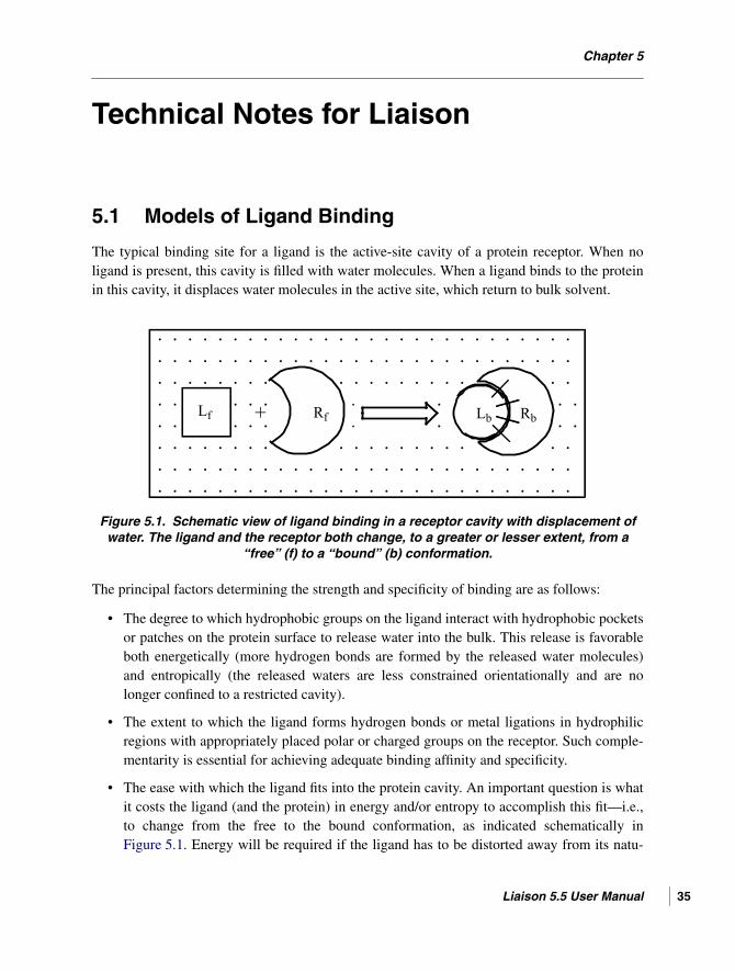
Liaison User Manual
Chapter 5
Chapter 5: Technical Notes for Liaison
5.1 Models of Ligand Binding
The typical binding site for a ligand is the active-site cavity of a protein receptor. When noligand is present, this cavity is filled with water molecules. When a ligand binds to the proteinin this cavity, it displaces water molecules in the active site, which return to bulk solvent.
Figure 5.1. Schematic view of ligand binding in a receptor cavity with displacement ofwater. The ligand and the receptor both change, to a greater or lesser extent, from a
“free” (f) to a “bound” (b) conformation.
The principal factors determining the strength and specificity of binding are as follows:
• The degree to which hydrophobic groups on the ligand interact with hydrophobic pocketsor patches on the protein surface to release water into the bulk. This release is favorableboth energetically (more hydrogen bonds are formed by the released water molecules)and entropically (the released waters are less constrained orientationally and are nolonger confined to a restricted cavity).
• The extent to which the ligand forms hydrogen bonds or metal ligations in hydrophilicregions with appropriately placed polar or charged groups on the receptor. Such comple-mentarity is essential for achieving adequate binding affinity and specificity.
• The ease with which the ligand fits into the protein cavity. An important question is whatit costs the ligand (and the protein) in energy and/or entropy to accomplish this fit—i.e.,to change from the free to the bound conformation, as indicated schematically inFigure 5.1. Energy will be required if the ligand has to be distorted away from its natu-
Lb RbRf+
. . . . . . . . . . . . . . . . . . . . . . . . . . . .
. . . . . . . . . . . . . . . . . . . . . . . . . . . .
. . . . . . . . . . . . . . . . . . .
. . . . . . . . .
. . . . . . . . .
. . . . . . . . . . . . . . . . . . .
. . . . . . . . . . . . . . . . . . . . . . . . . . . .
. . . . . . . . . . . . . . . . . . . . . . . . . . . .
Lf
Liaison 5.5 User Manual 35

Chapter 5: Technical Notes for Liaison
36
rally preferred, low-energy conformation into a higher-energy conformation when itbinds to the receptor. At the same time, entropy will be lost if the ligand is very flexible insolution and then is confined to a small number of conformations in the receptor cavity.Both effects, as well as similar restrictions on the conformation of protein side chains, actagainst binding.
5.1.1 Limitations of Free-Energy Perturbation
Molecular simulation methods have been used to calculate binding free energies of protein-ligand calculations since the pioneering applications of free energy perturbation (FEP)approaches by McCammon, Kollman, Jorgensen, and others approximately 20 years ago.During the past two decades, many FEP calculations have been carried out in academic groupsand in pharmaceutical and biotechnology companies. But while notable successes have beenachieved, FEP methods are in limited use in drug-discovery projects, for several reasons:
• FEP calculations are typically limited to small changes in ligand structure, restricting theapplicability to the very last phase of lead optimization.
• FEP calculations are very expensive computationally, and often cannot be completed on atime scale compatible with the schedule of a given drug-discovery project.
• Inaccuracies in force fields and sampling methods can lead to errors in FEP predictions.
5.1.2 Advantages of Linear Response Methods
The limitations of FEP motivated the development of linear-response (LR) methods by Aqvistseveral years ago (Hansson, T.; Aqvist, J. Protein Eng. 1995, 8, 1137–1145). Since that time,studies by Jorgensen and others have shown that LR methods can effectively address the abovedifficulties. In comparison with the FEP approach, the advantages of LRM are as follows:
• In contrast to FEP, where a large number of intermediate “windows” must be evaluated,LRM requires simulations only of the ligand in solution and the ligand bound to the pro-tein. The idea is that one views the binding event as replacement of the aqueous environ-ment of the ligand with a mixed aqueous/protein environment.
• Only interactions between the ligand and either the protein or the aqueous environmententer into the quantities that are accumulated during the simulation. The protein-proteinand protein-water interaction are part of the “reference” Hamiltonian, and hence are usedto generate conformations in the simulation, but are not used as descriptors in the result-ant model for the binding free energy. This eliminates a considerable amount of noise inthe calculations—for example, that arising from variations in the total energy that resultbecause slightly different geometries of the protein are obtained for each ligand moleculesimulated.
Liaison 5.5 User Manual
Chapter 5: Technical Notes for Liaison
• As long as the binding modes of the ligand are fundamentally similar, LRM calculationscan be applied to ligands that differ significantly in chemical structure.
• LRM calculations are less computationally expensive than FEP calculations.
• The LRM approach allows the binding-energy model to be calibrated by using a trainingset of compounds for which experimental binding affinities are known. The use of theenergy terms as descriptors in the fitting equation introduces an empirical element thatallows some of the limitations in the theoretical framework (for example, the neglect ofthe cost in energy and entropy of fitting the ligand into the protein site) and the physicalrepresentation (as reflected by errors in the force field or solvation model) to be partiallyabsorbed into the parameterization. Moreover, some of the steps involved in the bindingevent, such as the removal of water from the protein cavity and subsequent introductionof the ligand, are not inherently linear. If the linear-response approximation was rigor-ously valid, the coefficients of the terms would each be 0.5, corresponding to the mean-value approximation to the “charging” integral. In practice, optimization of the fittingparameters yields coefficients that are significantly different from the ideal value of 0.5.This empirical element sacrifices generality: the method probably requires the ligands tohave similar binding modes, and new parameters must be developed for each receptor. Inreturn, one can obtain a reasonable level of accuracy with a modest expenditure of CPUtime, under assumptions that are quite reasonable for many structure-based drug-designprojects.
5.1.3 Advantages of Liaison
Liaison—Schrödinger’s continuum-solvent implementation of LRM—has a number of highlyattractive features in addition to those listed in Section 5.1.2:
• The use of the Surface Generalized Born (SGB) continuum model greatly speeds the cal-culation because the various interaction terms converge much faster than in an explicit-solvent simulation. As a result, the required CPU time is reduced by a factor of 10 ormore.
• An even greater reduction in computational effort can be achieved by using a simpleenergy minimization protocol, rather than a molecular dynamics or Hybrid Monte Carlosimulation, and obtaining the LRM fitting data from the lowest-energy point reached bythe minimization. While there is sometimes a small degradation of accuracy as comparedto a simulation, the speed of the calculation is qualitatively enhanced.
• When “energy-minimization” sampling is coupled with a highly efficient TruncatedNewton minimizer, Liaison calculations are fast enough to be applied routinely in a con-temporary drug-discovery context. This approach makes Liaison very attractive forscreening a large number of ligands.
Liaison 5.5 User Manual 37

Chapter 5: Technical Notes for Liaison
38
• Schrödinger’s automatic atom-typing scheme for the OPLS-AA force field (Jorgensen,W. L.; Maxwell, D. S.; Tirado-Rives, J. J. Am. Chem. Soc. 1996, 118, 11223–11235)assigns charges, van der Waals, and valence parameters with no human intervention. Akey feature of OPLS-AA is that, via fitting to liquid-state simulations, excellent reproduc-tion of condensed-phase properties is obtained.
The Maestro graphical user interface makes it easy to set up and run Liaison calculations. First,a training set of compounds for which experimental binding affinities are available can be usedto generate simulation data that are then employed to determine the optimal LRM parameters.Once the parameters have been determined, libraries of compounds with unknown bindingaffinities can be run and their binding affinities can be predicted. Alternatively, Liaison canperform scoring on relaxed protein-ligand complexes, allowing direct prediction of ligandbinding energies.
It is important that the protein structures be correctly prepared. See the Protein PreparationGuidefor a description of Schrödinger’s protein-preparation facility.
5.2 LiaisonScore Binding Free Energy Model
Liaison calculates a scoring function, similar to GlideScore 3.5 SP, over the course of the LRMsimulation. This function, previously known as “GlideScore in Liaison” is now called Liaison-Score. The average LiaisonScore found in the simulation can be used to predict binding ener-gies using the formula
∆G = a(<LiaisonScore>) + b
instead of the LRM equation described above. The LiaisonScore binding energy model can beselected in the Analysis tab. The Analyze task can then be used to derive values for the a and bfitting coefficients.
This capability allows Liaison to be employed in the early stages of a drug-discovery project,i.e., before a set of ligands with known binding affinities suitable for training a LRM model isavailable. This approach transcends scoring in Glide itself because it allows the protein site torelax and enables the ligand to undergo full (not just torsional and rigid-body) optimization.
Advantages of LiaisonScore
Recall that docking with Glide is normally done with the vdW radii of non-polar ligand and/orprotein atoms scaled back by 10 to 20%. This rescaling creates more room in the rigid proteinsite and implicitly allows for “breathing motions” a protein site may carry out to accommodatea ligand that is slightly larger in some dimension than the ligand co-crystallized with theprotein. But while some protein sites may readily expand (or contract) upon ligand binding,others may be less adaptable, and the device of rescaling radii used by Glide will miss this
Liaison 5.5 User Manual

Chapter 5: Technical Notes for Liaison
distinction. Moreover, Glide further compensates for the limitations of docking into a rigidprotein site by allowing intramolecular contacts within the docked ligand pose to be shorterthan are physically realistic. These two aspects mean that Glide at times will give good scoresto ligands that are too large to bind in a given receptor site. There can also be cases in whichthe rigid site is somewhat too large for an active binder, particularly with the scaling down ofnon-polar radii. As a result an active ligand may score more poorly than it should.
In principle, such false positives and false negatives can be eliminated by repeating the Glidescoring after relaxing the ligand-protein complex. In this way, if the protein can readily adaptto the true (not Glide compacted) size and shape of the docked ligand, the recomputedGlideScore value should be good. But if the protein site cannot respond appropriately, a poorre-scored GlideScore value should be obtained. Note, however, that sites that are much toosmall will simply generate incorrect docked poses, and minimization will not transform such apose into a correctly docked structure.
Calibration of GlideScores
If a training set of ligands with known binding affinities is available, calibrated GlideScorevalues can be obtained as
GlideScore(calibrated)i = a GlideScore(raw)i + b (1)
Calibration has no effect on the rank order of calculated binding affinities or on the computedcorrelation coefficient, but can place the computed GlideScores on the correct experimentalscale and make it easier to interpret the calculated values.
5.3 Application to HIV Reverse Transcriptase
The Jorgensen group has been a leader in the development and testing of linear-responseapproaches for systems of pharmaceutical interest using explicit-solvent methods. An initialapplication to HIV reverse transcriptase examined the binding of 20 HEPT and 20 nevirapineanalogs (J. Med. Chem. 2001, 44, 145–154). More recently, this work has been extended toencompass 200 different inhibitors covering 8 chemical classes (J. Med. Chem. 2002, 45,2970–2987). Nevirapine is a FDA-approved anti-HIV drug of the non-nucleoside inhibitorclass, and one of the HEPT analogs (MKC-442) has been in clinical trials. As shown inFigure 5.2, the variation in the R2 sidechain is particularly sizable, ranging from hydrogen tomethyl benzyl ether. It would be very difficult, and very time consuming, to examine structuralvariations of this magnitude using free-energy perturbation methods.
Liaison 5.5 User Manual 39
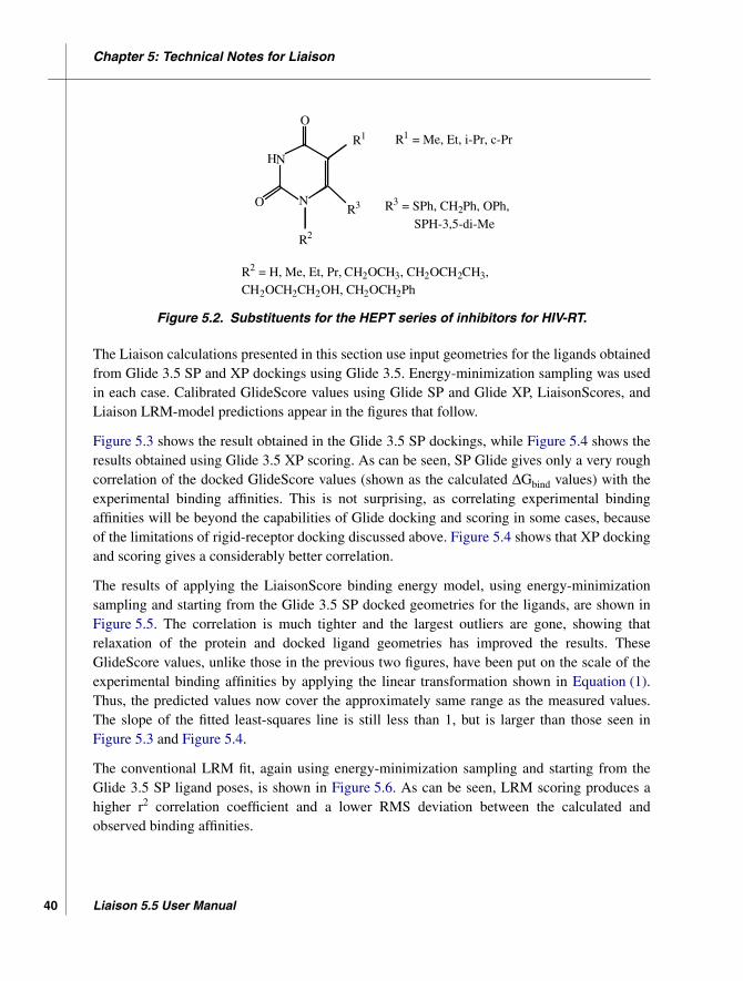
Chapter 5: Technical Notes for Liaison
40
Figure 5.2. Substituents for the HEPT series of inhibitors for HIV-RT.
The Liaison calculations presented in this section use input geometries for the ligands obtainedfrom Glide 3.5 SP and XP dockings using Glide 3.5. Energy-minimization sampling was usedin each case. Calibrated GlideScore values using Glide SP and Glide XP, LiaisonScores, andLiaison LRM-model predictions appear in the figures that follow.
Figure 5.3 shows the result obtained in the Glide 3.5 SP dockings, while Figure 5.4 shows theresults obtained using Glide 3.5 XP scoring. As can be seen, SP Glide gives only a very roughcorrelation of the docked GlideScore values (shown as the calculated ∆Gbind values) with theexperimental binding affinities. This is not surprising, as correlating experimental bindingaffinities will be beyond the capabilities of Glide docking and scoring in some cases, becauseof the limitations of rigid-receptor docking discussed above. Figure 5.4 shows that XP dockingand scoring gives a considerably better correlation.
The results of applying the LiaisonScore binding energy model, using energy-minimizationsampling and starting from the Glide 3.5 SP docked geometries for the ligands, are shown inFigure 5.5. The correlation is much tighter and the largest outliers are gone, showing thatrelaxation of the protein and docked ligand geometries has improved the results. TheseGlideScore values, unlike those in the previous two figures, have been put on the scale of theexperimental binding affinities by applying the linear transformation shown in Equation (1).Thus, the predicted values now cover the approximately same range as the measured values.The slope of the fitted least-squares line is still less than 1, but is larger than those seen inFigure 5.3 and Figure 5.4.
The conventional LRM fit, again using energy-minimization sampling and starting from theGlide 3.5 SP ligand poses, is shown in Figure 5.6. As can be seen, LRM scoring produces ahigher r2 correlation coefficient and a lower RMS deviation between the calculated andobserved binding affinities.
O
O
NH
N
R1
R2
R3
R1 = Me, Et, i-Pr, c-Pr
R3 = SPh, CH2Ph, OPh, SPH-3,5-di-Me
R2 = H, Me, Et, Pr, CH2OCH3, CH2OCH2CH3,CH2OCH2CH2OH, CH2OCH2Ph
Liaison 5.5 User Manual

Chapter 5: Technical Notes for Liaison
Figure 5.3. Correlation of calculated (GlideScore) and observed binding affinities forGlide 3.5 SP docking of HEPT inhibitors into HIV reverse transcriptase.
Figure 5.4. Correlation of calculated (GlideScore) and observed binding affinities forGlide 3.5 XP docking of HEPT inhibitors into HIV reverse transcriptase.
-13 -12 -11 -10 -9 -8 -7 -6 -5-10
-9
-8
-7
r2 = 0.32
Experimental ∆Gbind (kcal/mol)
Cal
c.∆
Gb
ind (
kcal
/mo
l)
-13 -12 -11 -10 -9 -8 -7 -6 -5-16
-15
-14
-13
-12
r2 = 0.60
Experimental ∆Gbind (kcal/mol)
Cal
c.∆
Gb
ind (
kcal
/mo
l)
Liaison 5.5 User Manual 41

Chapter 5: Technical Notes for Liaison
42
Figure 5.5. Correlation of LiaisonScores for the HEPT inhibitors forHIV reverse transcriptase, calculated by energy-minimization sampling starting from
Glide 3.5 SP docked geometries.
Figure 5.6. Correlation of Liaison LRM scoring for the HEPT series of inhibitors for HIVreverse transcriptase, calculated by energy-minimization sampling starting from Glide
3.5 SP docked geometries.
-13 -12 -11 -10 -9 -8 -7 -6 -5-14
-13
-12
-11
-10
-9
-8
-7
-6
-5
r2 = 0.77RMSD = 1.08 kcal/mol
Experimental ∆Gbind (kcal/mol)
Cal
c.∆
Gb
ind (
kcal
/mo
l)
-13 -12 -11 -10 -9 -8 -7 -6 -5-13
-12
-11
-10
-9
-8
-7
-6
-5
r2 = 0.82RMSD = 1.01 kcal/mol
Experimental ∆Gbind (kcal/mol)
Cal
c.∆
Gb
ind (
kcal
/mo
l)
Liaison 5.5 User Manual

Chapter 5: Technical Notes for Liaison
These results suggest that some of the limitations expected for rigid-receptor docking can beaddressed by relaxing the docked complexes before scoring them with GlideScore or via astandard LRM fitting model. LRM scoring gives the best results in this instance, but it remainsto be seen whether this will always be the case.
Normally we would expect even better results from energy-minimization sampling followedby rescoring in Liaison when starting from the XP-docked poses. This indeed is our recom-mended procedure. In this instance, however, the results obtained using the same two modelsgives correlations that are better than those shown in Figure 5.3 but are not as good as those inFigure 5.4 and Figure 5.5. This is counterintuitive, especially in view of the fact that XP docksonly one ligand in a manner that is inconsistent with the other cases, and here the variationmerely consists of a reversal of the positions adopted by the pseudo-symmetric C-R1 and N-R2groups (see Figure 5.2). In contrast, SP Glide docks three ligands in an inconsistent, andpresumably incorrect, manner.
5.4 Application to ß-Secretase (BACE) Inhibitors
Tounge and Reynolds (J. Med. Chem. 2003, 46, 2074–2082) recently reported the applicationof Liaison to ten β-secretase inhibitors of the general structure shown in Figure 5.7, where R1
is typically a BOC-capped dipeptide, and R2 and R3 are usually methyl or isopropyl. Theseneutral inhibitors have relatively high molecular weights and resemble HIV protease ligands instructure. Tounge and Reynolds also studied two nanomolar co-crystallized octapeptides thathave two or three aspartate or glutamate residues and hence are negatively charged at physio-logical pH.
Figure 5.7. Schematic structure of neutral BACE inhibitors studied by Tounge andReynolds.
N NN
O
O O
H
H
R1
R2
R3
H
H
Ph
Liaison 5.5 User Manual 43

Chapter 5: Technical Notes for Liaison
44
Figure 5.8. Correlation of predicted and observed binding affinities for BACE inhibitorsusing LRM scoring and energy-minimization sampling.
A plot of their data for energy-minimization sampling, taken from Figure 5 in their paper, ispresented in Figure 5.8; hybrid Monte Carlo sampling gave a similar result. The correlation isreasonably good, but the negatively charged octapeptides (the two data points with the mostnegative calculated and observed binding affinities) fall off the line. This is not surprising, as itis notoriously difficult in binding energy correlations to get ligands having different chargestates to fall on a common line.
Tounge and Reynolds also presented results for other simulation conditions that gave poorerfits to the experimental data. We nevertheless regard their results as promising, and intend toemploy their series of BACE inhibitors in future efforts to improve Liaison.
-14 -13 -12 -11 -10 -9 -8 -7 -6-14
-13
-12
-11
-10
-9
-8
Experimental ∆Gbind (kcal/mol)
Cal
c.∆
Gb
ind (
kcal
/mo
l)
r2 = 0.61RMSD = 1.10
Liaison 5.5 User Manual

Liaison User Manual
Getting Help
Schrödinger software is distributed with documentation in PDF format. If the documentation isnot installed in $SCHRODINGER/docs on a computer that you have access to, you should installit or ask your system administrator to install it.
For help installing and setting up licenses for Schrödinger software and installing documenta-tion, see the Installation Guide. For information on running jobs, see the Job Control Guide.
Maestro has automatic, context-sensitive help (Auto-Help and Balloon Help, or tooltips), andan online help system. To get help, follow the steps below.
• Check the Auto-Help text box, which is located at the foot of the main window. If help isavailable for the task you are performing, it is automatically displayed there. Auto-Helpcontains a single line of information. For more detailed information, use the online help.
• If you want information about a GUI element, such as a button or option, there may beBalloon Help for the item. Pause the cursor over the element. If the Balloon Help doesnot appear, check that Show Balloon Help is selected in the Maestro menu of the mainwindow. If there is Balloon Help for the element, it appears within a few seconds.
• For information about a panel or the tab that is displayed in a panel, click the Help buttonin the panel, or press F1. The help topic is displayed in your browser.
• For other information in the online help, open the default help topic by choosing OnlineHelp from the Help menu on the main menu bar or by pressing CTRL+H. This topic is dis-played in your browser. You can navigate to topics in the navigation bar.
The Help menu also provides access to the manuals (including a full text search), the FAQpages, the New Features pages, and several other topics.
If you do not find the information you need in the Maestro help system, check the followingsources:
• Maestro User Manual, for detailed information on using Maestro• Maestro Command Reference Manual, for information on Maestro commands• Maestro Overview, for an overview of the main features of Maestro• Maestro Tutorial, for a tutorial introduction to basic Maestro features• Impact User Manual, for detailed information on basic Impact tasks and panels• Impact Command Reference Manual, for Impact command syntax• Strike User Manual, for detailed information on using Strike
Liaison 5.5 User Manual 45

Getting Help
46
• Ligand & Structure-Based Descriptors, for information on using Liaison for descriptors• Liaison Frequently Asked Questions pages, at
https://www.schrodinger.com/Liaison_FAQ.html• Known Issues pages, available on the Support Center.
The manuals are also available in PDF format from the Schrödinger Support Center. Localcopies of the FAQs and Known Issues pages can be viewed by opening the fileSuite_2009_Index.html, which is in the docs directory of the software installation, andfollowing the links to the relevant index pages.
Information on available scripts can be found on the Script Center. Information on availablesoftware updates can be obtained by choosing Check for Updates from the Maestro menu.
If you have questions that are not answered from any of the above sources, contact Schrödingerusing the information below.
E-mail: [email protected]: Schrödinger, 101 SW Main Street, Suite 1300, Portland, OR 97204Phone: (503) 299-1150Fax: (503) 299-4532WWW: http://www.schrodinger.comFTP: ftp://ftp.schrodinger.com
Generally, e-mail correspondence is best because you can send machine output, if necessary.When sending e-mail messages, please include the following information:
• All relevant user input and machine output• Liaison purchaser (company, research institution, or individual)• Primary Liaison user• Computer platform type• Operating system with version number• Liaison version number• Maestro version number• mmshare version number
On UNIX you can obtain the machine and system information listed above by entering thefollowing command at a shell prompt:
$SCHRODINGER/utilities/postmortem
This command generates a file named username-host-schrodinger.tar.gz, which youshould send to [email protected]. If you have a job that failed, enter the followingcommand:
$SCHRODINGER/utilities/postmortem jobid
Liaison 5.5 User Manual

Getting Help
where jobid is the job ID of the failed job, which you can find in the Monitor panel. Thiscommand archives job information as well as the machine and system information, andincludes input and output files (but not structure files). If you have sensitive data in the joblaunch directory, you should move those files to another location first. The archive is namedjobid-archive.tar.gz, and should be sent to [email protected] Maestro fails, anerror report that contains the relevant information is written to the current working directory.The report is named maestro_error.txt, and should be sent to [email protected]. Amessage giving the location of this file is written to the terminal window.
More information on the postmortem command can be found in Appendix A of the JobControl Guide.
Liaison 5.5 User Manual 47

48
Liaison 5.5 User Manual
Index
Aactive-site cavity................................................ 35adding hydrogens .............................................. 26all-atom force field.............................................. 1Analysis tab
Liaison panel .............................................. 32analysis task ...................................................... 27
Bbinding energy model
LiaisonScore ........................................... 3, 38LRM ............................................................. 2
bonds, covalent, to receptor .............................. 23
Ccavity, active site ............................................... 35close contacts .................................................... 22command line, running Liaison from................ 33conventions, document........................................ v
Ddirectory
installation .................................................... 3Maestro working........................................... 3
Eenvironment variable, SCHRODINGER ................. 3
Ffitting task ........................................................... 1
example....................................................... 11overview ..................................................... 28
force field ...................................................... 1, 31format conversion, to Maestro .......................... 26free energy perturbation (FEP) ......................... 36frozen residues .................................................. 32
Hhydrogen treatment ........................................... 26
Iidentical chains.................................................. 20
LLIA equation ....................................................... 2Liaison panel
Analysis tab .......................................... 10, 32Parameters tab............................................. 31Systems tab............................................. 7, 29
LiaisonScore ................................................. 3, 38license, LigPrep................................................. 24ligand binding, schematic view......................... 35LigPrep........................................................ 24–26linear-response (LR) methods........................... 36LRM binding energy model................................ 2
MMaestro
introduction to .............................................. 1starting .......................................................... 3
metalloproteins, charge and protonation states . 24metals
adjusting charges ........................................ 20coordination of ligands to ........................... 24covalent bonds to protein............................ 20
multimeric protein structures ............................ 19
OOPLS-AA force fields......................................... 1overview of protein preparation ........................ 19
PParameters tab
Liaison panel .............................................. 31prediction task..................................................... 1
example....................................................... 13overview ..................................................... 28
product installation............................................ 45protein
adjustment of structure ............................... 20misprotonation of........................................ 22
protein preparation, overview ........................... 19protonation state................................................ 23
SSchrödinger contact information....................... 46simulation method............................................. 30simulation task .................................................. 27
Liaison 5.5 User Manual 49

50
Index
solvation model ............................................. 2, 31Strike ....................................................... 1, 27, 32
Build QSAR Model panel .......................... 12Predict based on QSAR model panel ......... 14Univariate and Bivariate statistics panel..... 15
structuresformat conversion ....................................... 26requirements for docking............................ 23
Surface Generalized Born (SGB) solvent model 2Systems tab, Liaison panel................................ 29
Liaison 5.5 User Manual


120 West 45th Street, 29th Floor
New York, NY 10036
101 SW Main Street, Suite 1300
Portland, OR 97204
8910 University Center Lane, Suite 270
San Diego, CA 92122
Zeppelinstraße 13
81669 München, Germany
Dynamostraße 13
68165 Mannheim, Germany
Quatro House, Frimley Road
Camberley GU16 7ER, United Kingdom
SCHRÖDINGER ®