libmesh - the institute for computational engineering and...
TRANSCRIPT
Introduction Applications Weighted Residuals Finite Elements Essential BCs Complex Problems Adaptivity
LibMesh
Roy H. Stogner John W. [email protected] [email protected]
Univ. of Texas at Austin
June 6, 2007
Introduction Applications Weighted Residuals Finite Elements Essential BCs Complex Problems Adaptivity
Outline
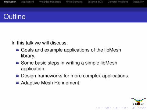
In this talk we will discuss:Goals and example applications of the libMeshlibrary.Some basic steps in writing a simple libMeshapplication.Design frameworks for more complex applications.Adaptive Mesh Refinement.
Introduction Applications Weighted Residuals Finite Elements Essential BCs Complex Problems Adaptivity
Outline
In this talk we will discuss:Goals and example applications of the libMeshlibrary.Some basic steps in writing a simple libMeshapplication.Design frameworks for more complex applications.Adaptive Mesh Refinement.
Introduction Applications Weighted Residuals Finite Elements Essential BCs Complex Problems Adaptivity
Goals
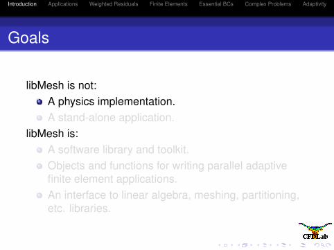
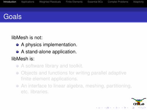
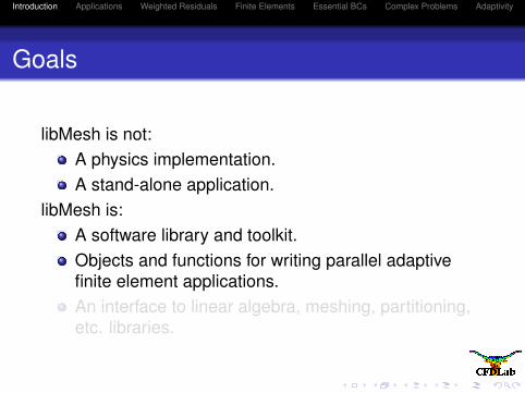
libMesh is not:A physics implementation.A stand-alone application.
libMesh is:A software library and toolkit.Objects and functions for writing parallel adaptivefinite element applications.An interface to linear algebra, meshing, partitioning,etc. libraries.
Introduction Applications Weighted Residuals Finite Elements Essential BCs Complex Problems Adaptivity
Goals
libMesh is not:A physics implementation.A stand-alone application.
libMesh is:A software library and toolkit.Objects and functions for writing parallel adaptivefinite element applications.An interface to linear algebra, meshing, partitioning,etc. libraries.
Introduction Applications Weighted Residuals Finite Elements Essential BCs Complex Problems Adaptivity
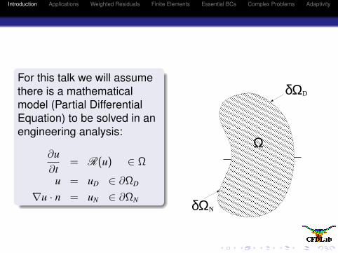
For this talk we will assumethere is a mathematicalmodel (Partial DifferentialEquation) to be solved in anengineering analysis:
∂u∂t
= R(u) ∈ Ω
u = uD ∈ ∂ΩD
∇u · n = uN ∈ ∂ΩN
δΩD
δΩN
Ω
Introduction Applications Weighted Residuals Finite Elements Essential BCs Complex Problems Adaptivity
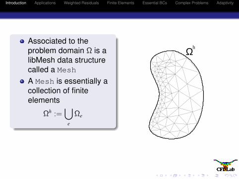
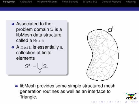
Associated to theproblem domain Ω is alibMesh data structurecalled a Mesh
A Mesh is essentially acollection of finiteelements
Ωh :=⋃
e
Ωe
Ωh
libMesh provides some simple structured meshgeneration routines as well as an interface toTriangle.
Introduction Applications Weighted Residuals Finite Elements Essential BCs Complex Problems Adaptivity
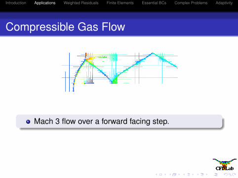
Compressible Gas Flow
Mach 3 flow over a forward facing step.
Introduction Applications Weighted Residuals Finite Elements Essential BCs Complex Problems Adaptivity
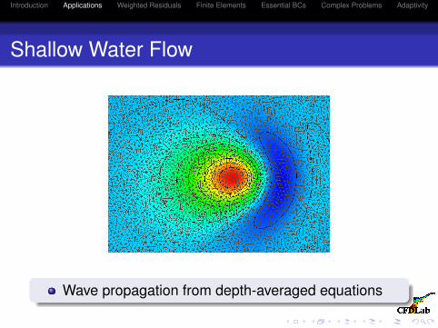
Shallow Water Flow
Wave propagation from depth-averaged equations
Introduction Applications Weighted Residuals Finite Elements Essential BCs Complex Problems Adaptivity
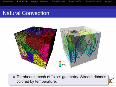
Natural Convection
Tetrahedral mesh of “pipe” geometry. Stream ribbonscolored by temperature.
Introduction Applications Weighted Residuals Finite Elements Essential BCs Complex Problems Adaptivity
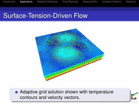
Surface-Tension-Driven Flow
Adaptive grid solution shown with temperaturecontours and velocity vectors.
Introduction Applications Weighted Residuals Finite Elements Essential BCs Complex Problems Adaptivity
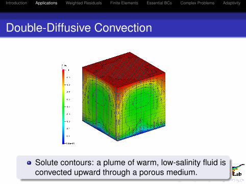
Double-Diffusive Convection
Solute contours: a plume of warm, low-salinity fluid isconvected upward through a porous medium.
Introduction Applications Weighted Residuals Finite Elements Essential BCs Complex Problems Adaptivity
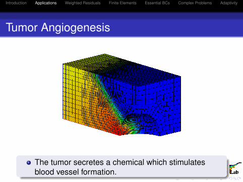
Tumor Angiogenesis
The tumor secretes a chemical which stimulatesblood vessel formation.
Introduction Applications Weighted Residuals Finite Elements Essential BCs Complex Problems Adaptivity
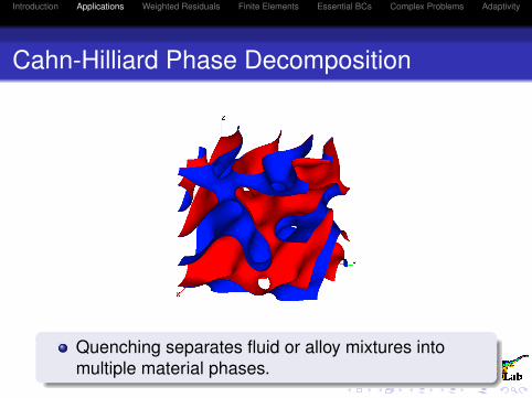
Cahn-Hilliard Phase Decomposition
Quenching separates fluid or alloy mixtures intomultiple material phases.
Introduction Applications Weighted Residuals Finite Elements Essential BCs Complex Problems Adaptivity
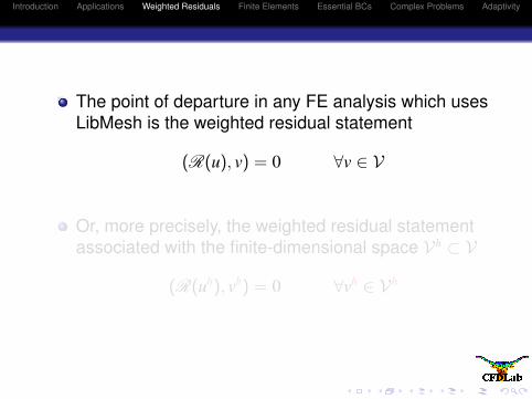
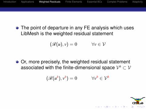
The point of departure in any FE analysis which usesLibMesh is the weighted residual statement
(R(u), v) = 0 ∀v ∈ V
Or, more precisely, the weighted residual statementassociated with the finite-dimensional space Vh ⊂ V
(R(uh), vh) = 0 ∀vh ∈ Vh
Introduction Applications Weighted Residuals Finite Elements Essential BCs Complex Problems Adaptivity
The point of departure in any FE analysis which usesLibMesh is the weighted residual statement
(R(u), v) = 0 ∀v ∈ V
Or, more precisely, the weighted residual statementassociated with the finite-dimensional space Vh ⊂ V
(R(uh), vh) = 0 ∀vh ∈ Vh

Introduction Applications Weighted Residuals Finite Elements Essential BCs Complex Problems Adaptivity
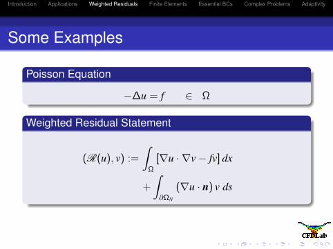
Some Examples
Poisson Equation
−∆u = f ∈ Ω
Introduction Applications Weighted Residuals Finite Elements Essential BCs Complex Problems Adaptivity
Some Examples
Poisson Equation
−∆u = f ∈ Ω
Weighted Residual Statement
(R(u), v) :=
∫Ω
[∇u · ∇v− fv] dx
+
∫∂ΩN
(∇u · n) v ds
Introduction Applications Weighted Residuals Finite Elements Essential BCs Complex Problems Adaptivity
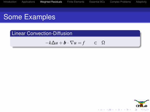
Some Examples
Linear Convection-Diffusion
−k∆u + b · ∇u = f ∈ Ω
Introduction Applications Weighted Residuals Finite Elements Essential BCs Complex Problems Adaptivity
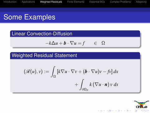
Some Examples
Linear Convection-Diffusion
−k∆u + b · ∇u = f ∈ Ω
Weighted Residual Statement
(R(u), v) :=
∫Ω
[k∇u · ∇v + (b · ∇u)v− fv] dx
+
∫∂ΩN
k (∇u · n) v ds

Introduction Applications Weighted Residuals Finite Elements Essential BCs Complex Problems Adaptivity
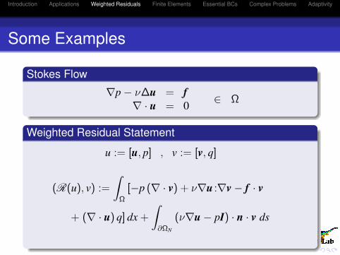
Some Examples
Stokes Flow
∇p− ν∆u = f∇ · u = 0 ∈ Ω
Introduction Applications Weighted Residuals Finite Elements Essential BCs Complex Problems Adaptivity
Some Examples
Stokes Flow
∇p− ν∆u = f∇ · u = 0 ∈ Ω
Weighted Residual Statement
u := [u, p] , v := [v, q]
(R(u), v) :=
∫Ω
[−p (∇ · v) + ν∇u :∇v− f · v
+ (∇ · u) q] dx +
∫∂ΩN
(ν∇u− pI) · n · v ds

Introduction Applications Weighted Residuals Finite Elements Essential BCs Complex Problems Adaptivity
To obtain the approximate problem, we simplyreplace u← uh, v← vh, and Ω← Ωh in the weightedresidual statement.
Introduction Applications Weighted Residuals Finite Elements Essential BCs Complex Problems Adaptivity
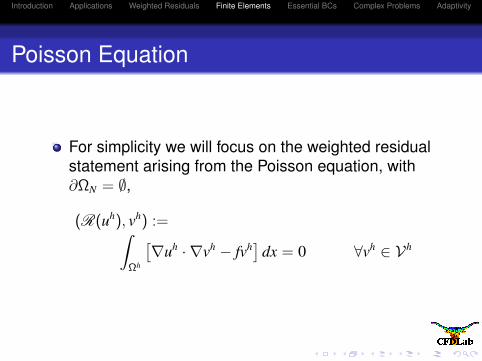
Poisson Equation
For simplicity we will focus on the weighted residualstatement arising from the Poisson equation, with∂ΩN = ∅,
(R(uh), vh) :=∫Ωh
[∇uh · ∇vh − fvh] dx = 0 ∀vh ∈ Vh

Introduction Applications Weighted Residuals Finite Elements Essential BCs Complex Problems Adaptivity
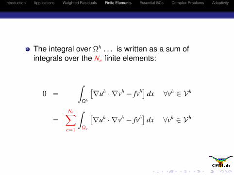
The integral over Ωh . . .
is written as a sum ofintegrals over the Ne finite elements:
0 =
∫Ωh
[∇uh · ∇vh − fvh] dx ∀vh ∈ Vh
=Ne∑
e=1
∫Ωe
[∇uh · ∇vh − fvh] dx ∀vh ∈ Vh
Introduction Applications Weighted Residuals Finite Elements Essential BCs Complex Problems Adaptivity
The integral over Ωh . . . is written as a sum ofintegrals over the Ne finite elements:
0 =
∫Ωh
[∇uh · ∇vh − fvh] dx ∀vh ∈ Vh
=Ne∑
e=1
∫Ωe
[∇uh · ∇vh − fvh] dx ∀vh ∈ Vh
Introduction Applications Weighted Residuals Finite Elements Essential BCs Complex Problems Adaptivity
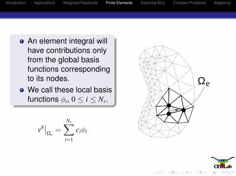
An element integral willhave contributions onlyfrom the global basisfunctions correspondingto its nodes.We call these local basisfunctions φi, 0 ≤ i ≤ Ns.
vh∣∣Ωe
=Ns∑
i=1
ciφi
∫Ωe
vh dx =Ns∑
i=1
ci
∫Ωe
φi dx
Ωe

Introduction Applications Weighted Residuals Finite Elements Essential BCs Complex Problems Adaptivity
An element integral willhave contributions onlyfrom the global basisfunctions correspondingto its nodes.We call these local basisfunctions φi, 0 ≤ i ≤ Ns.
vh∣∣Ωe
=Ns∑
i=1
ciφi
∫Ωe
vh dx =Ns∑
i=1
ci
∫Ωe
φi dx
Ωe
Introduction Applications Weighted Residuals Finite Elements Essential BCs Complex Problems Adaptivity
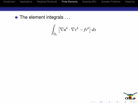
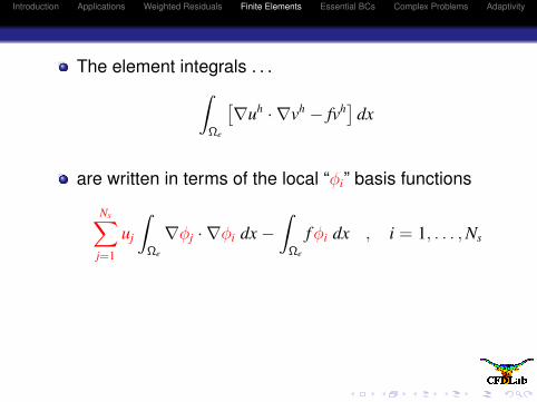
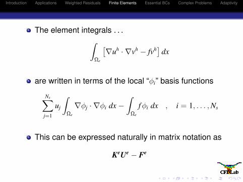
The element integrals . . .∫Ωe
[∇uh · ∇vh − fvh] dx
are written in terms of the local “φi” basis functions
Ns∑j=1
uj
∫Ωe
∇φj · ∇φi dx−∫
Ωe
f φi dx , i = 1, . . . , Ns
This can be expressed naturally in matrix notation as
KeUe − Fe
Introduction Applications Weighted Residuals Finite Elements Essential BCs Complex Problems Adaptivity
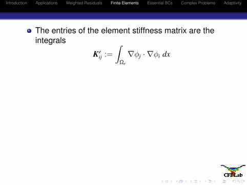
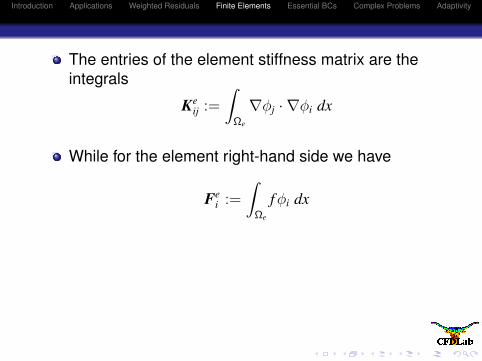
The entries of the element stiffness matrix are theintegrals
Keij :=
∫Ωe
∇φj · ∇φi dx
While for the element right-hand side we have
Fei :=
∫Ωe
f φi dx
The element stiffness matrices and right-hand sidescan be “assembled” to obtain the global system ofequations
KU = F
Introduction Applications Weighted Residuals Finite Elements Essential BCs Complex Problems Adaptivity
The entries of the element stiffness matrix are theintegrals
Keij :=
∫Ωe
∇φj · ∇φi dx
While for the element right-hand side we have
Fei :=
∫Ωe
f φi dx
The element stiffness matrices and right-hand sidescan be “assembled” to obtain the global system ofequations
KU = F
Introduction Applications Weighted Residuals Finite Elements Essential BCs Complex Problems Adaptivity
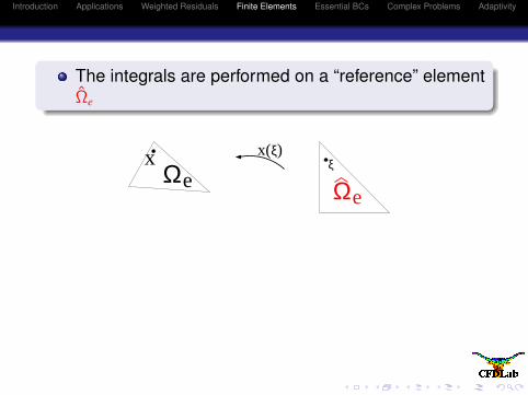
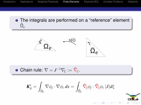
The integrals are performed on a “reference” elementΩe
eΩx ξ)x(
ξ
Ωe
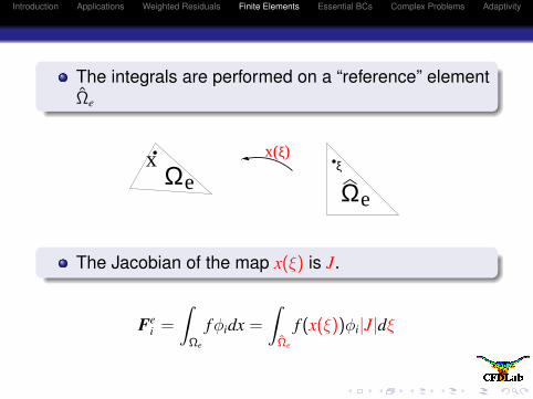
Introduction Applications Weighted Residuals Finite Elements Essential BCs Complex Problems Adaptivity
The integrals are performed on a “reference” elementΩe
eΩx x(ξ)
ξ
Ωe
The Jacobian of the map x(ξ) is J.
Fei =
∫Ωe
f φidx =
∫Ωe
f (x(ξ))φi|J|dξ
Introduction Applications Weighted Residuals Finite Elements Essential BCs Complex Problems Adaptivity
The integrals are performed on a “reference” elementΩe
eΩx ξ)x(
ξ
Ωe
Chain rule: ∇ = J−1∇ξ := ∇ξ.
Keij =
∫Ωe
∇φj · ∇φi dx =
∫Ωe
∇ξφj · ∇ξφi |J|dξ

Introduction Applications Weighted Residuals Finite Elements Essential BCs Complex Problems Adaptivity
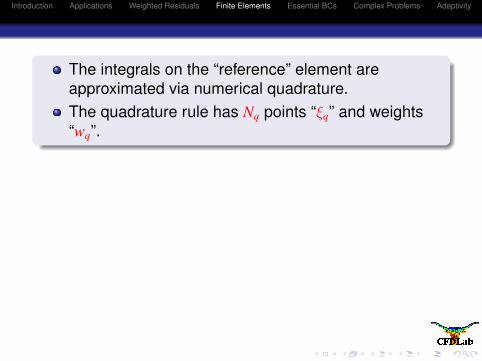
The integrals on the “reference” element areapproximated via numerical quadrature.
The quadrature rule has Nq points “ξq” and weights“wq”.
Introduction Applications Weighted Residuals Finite Elements Essential BCs Complex Problems Adaptivity
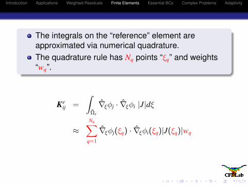
The integrals on the “reference” element areapproximated via numerical quadrature.The quadrature rule has Nq points “ξq” and weights“wq”.

Introduction Applications Weighted Residuals Finite Elements Essential BCs Complex Problems Adaptivity
The integrals on the “reference” element areapproximated via numerical quadrature.The quadrature rule has Nq points “ξq” and weights“wq”.
Fei =
∫Ωe
f φi|J|dξ
≈Nq∑
q=1
f (x(ξq))φi(ξq)|J(ξq)|wq
Introduction Applications Weighted Residuals Finite Elements Essential BCs Complex Problems Adaptivity
The integrals on the “reference” element areapproximated via numerical quadrature.The quadrature rule has Nq points “ξq” and weights“wq”.
Keij =
∫Ωe
∇ξφj · ∇ξφi |J|dξ
≈Nq∑
q=1
∇ξφj(ξq) · ∇ξφi(ξq)|J(ξq)|wq
Introduction Applications Weighted Residuals Finite Elements Essential BCs Complex Problems Adaptivity
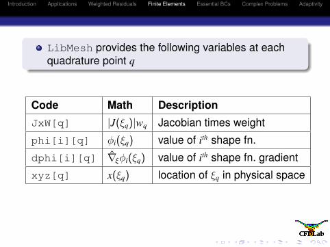
LibMesh provides the following variables at eachquadrature point q
Code Math Description
JxW[q] |J(ξq)|wq Jacobian times weight
phi[i][q] φi(ξq) value of ith shape fn.
dphi[i][q] ∇ξφi(ξq) value of ith shape fn. gradient
xyz[q] x(ξq) location of ξq in physical space
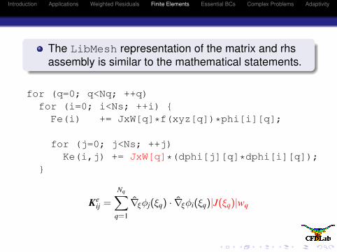
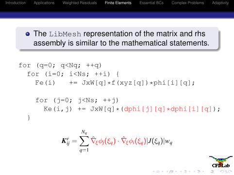
Introduction Applications Weighted Residuals Finite Elements Essential BCs Complex Problems Adaptivity
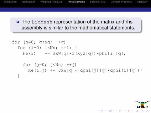
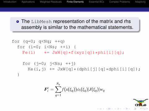
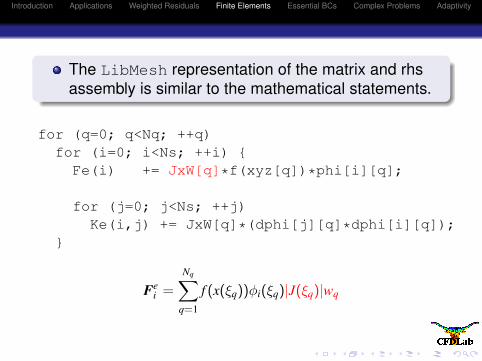
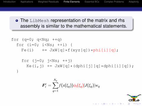
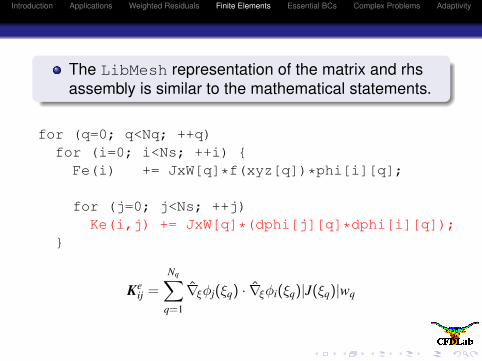
The LibMesh representation of the matrix and rhsassembly is similar to the mathematical statements.
for (q=0; q<Nq; ++q)for (i=0; i<Ns; ++i) Fe(i) += JxW[q]*f(xyz[q])*phi[i][q];
for (j=0; j<Ns; ++j)Ke(i,j) += JxW[q]*(dphi[j][q]*dphi[i][q]);
Introduction Applications Weighted Residuals Finite Elements Essential BCs Complex Problems Adaptivity
The LibMesh representation of the matrix and rhsassembly is similar to the mathematical statements.
for (q=0; q<Nq; ++q)for (i=0; i<Ns; ++i) Fe(i) += JxW[q]*f(xyz[q])*phi[i][q];
for (j=0; j<Ns; ++j)Ke(i,j) += JxW[q]*(dphi[j][q]*dphi[i][q]);
Fei =
Nq∑q=1
f (x(ξq))φi(ξq)|J(ξq)|wq
Introduction Applications Weighted Residuals Finite Elements Essential BCs Complex Problems Adaptivity
The LibMesh representation of the matrix and rhsassembly is similar to the mathematical statements.
for (q=0; q<Nq; ++q)for (i=0; i<Ns; ++i) Fe(i) += JxW[q]*f(xyz[q])*phi[i][q];
for (j=0; j<Ns; ++j)Ke(i,j) += JxW[q]*(dphi[j][q]*dphi[i][q]);
Fei =
Nq∑q=1
f (x(ξq))φi(ξq)|J(ξq)|wq
Introduction Applications Weighted Residuals Finite Elements Essential BCs Complex Problems Adaptivity
The LibMesh representation of the matrix and rhsassembly is similar to the mathematical statements.
for (q=0; q<Nq; ++q)for (i=0; i<Ns; ++i) Fe(i) += JxW[q]*f(xyz[q])*phi[i][q];
for (j=0; j<Ns; ++j)Ke(i,j) += JxW[q]*(dphi[j][q]*dphi[i][q]);
Keij =
Nq∑q=1
∇ξφj(ξq) · ∇ξφi(ξq)|J(ξq)|wq
Introduction Applications Weighted Residuals Finite Elements Essential BCs Complex Problems Adaptivity
The LibMesh representation of the matrix and rhsassembly is similar to the mathematical statements.
for (q=0; q<Nq; ++q)for (i=0; i<Ns; ++i) Fe(i) += JxW[q]*f(xyz[q])*phi[i][q];
for (j=0; j<Ns; ++j)Ke(i,j) += JxW[q]*(dphi[j][q]*dphi[i][q]);
Keij =
Nq∑q=1
∇ξφj(ξq) · ∇ξφi(ξq)|J(ξq)|wq

Introduction Applications Weighted Residuals Finite Elements Essential BCs Complex Problems Adaptivity
Object Oriented Programming
Abstract Base Classes define user interfaces.Concrete Subclasses implement functionality.One physics code can work with manydiscretizations.

Introduction Applications Weighted Residuals Finite Elements Essential BCs Complex Problems Adaptivity
Object Oriented Programming
Abstract Base Classes define user interfaces.Concrete Subclasses implement functionality.One physics code can work with manydiscretizations.

Introduction Applications Weighted Residuals Finite Elements Essential BCs Complex Problems Adaptivity
Object Oriented Programming
Abstract Base Classes define user interfaces.Concrete Subclasses implement functionality.One physics code can work with manydiscretizations.
Introduction Applications Weighted Residuals Finite Elements Essential BCs Complex Problems Adaptivity
Object Oriented Programming
Abstract Base Classes define user interfaces.Concrete Subclasses implement functionality.One physics code can work with manydiscretizations.
Introduction Applications Weighted Residuals Finite Elements Essential BCs Complex Problems Adaptivity
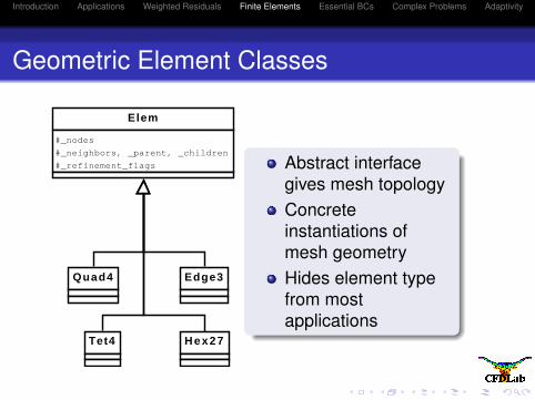
Geometric Element Classes
Elem
#_nodes
#_neighbors, _parent, _children
#_refinement_flags
Quad4
Tet4
Edge3
Hex27
Abstract interfacegives mesh topologyConcreteinstantiations ofmesh geometryHides element typefrom mostapplications

Introduction Applications Weighted Residuals Finite Elements Essential BCs Complex Problems Adaptivity
Finite Element Classes
FEBase
+phi, dphi, d2phi
+quadrature_rule, JxW
+reinit(Elem)
+reinit(Elem,side)
Lagrange
Hermi te
Hierarchic
Monomial
Finite Element objectbuilds data for eachGeometric objectUser only deals withshape function,quadrature data
Introduction Applications Weighted Residuals Finite Elements Essential BCs Complex Problems Adaptivity
For linear problems, we have already seen how theweighted residual statement leads directly to asparse linear system of equations
KU = F

Introduction Applications Weighted Residuals Finite Elements Essential BCs Complex Problems Adaptivity
For time-dependent problems,
∂u∂t
= R(u)
we also need a way to advance the solution in time,e.g. a θ-method(
un+1 − un
∆t, vh
)=
(R(uθ), vh) ∀vh ∈ Vh
uθ := θun+1 + (1− θ)un
Leads to KU = F at each timestep.
Introduction Applications Weighted Residuals Finite Elements Essential BCs Complex Problems Adaptivity
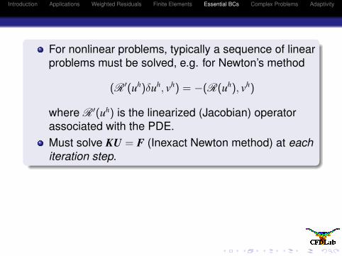
For nonlinear problems, typically a sequence of linearproblems must be solved, e.g. for Newton’s method
(R ′(uh)δuh, vh) = −(R(uh), vh)
where R ′(uh) is the linearized (Jacobian) operatorassociated with the PDE.Must solve KU = F (Inexact Newton method) at eachiteration step.
Introduction Applications Weighted Residuals Finite Elements Essential BCs Complex Problems Adaptivity
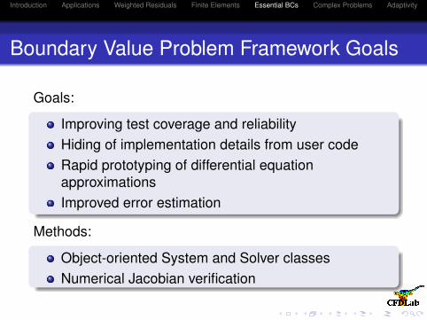
Boundary Value Problem Framework Goals
Goals:
Improving test coverage and reliabilityHiding of implementation details from user codeRapid prototyping of differential equationapproximationsImproved error estimation
Methods:
Object-oriented System and Solver classesNumerical Jacobian verification
Introduction Applications Weighted Residuals Finite Elements Essential BCs Complex Problems Adaptivity
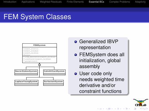
FEM System Classes
FEMSystem
+element_solution
+element_residual
+element_jacobian
+FE_base
+*_time_derivative(request_jacobian)
+*_constraint(request_jacobian)
+*_postprocess()
NavierStokesSystem
LaplaceYoungSystem
CahnHil l iardSystem
SurfactantSystem
Generalized IBVPrepresentationFEMSystem does allinitialization, globalassemblyUser code onlyneeds weighted timederivative and/orconstraint functions
Introduction Applications Weighted Residuals Finite Elements Essential BCs Complex Problems Adaptivity
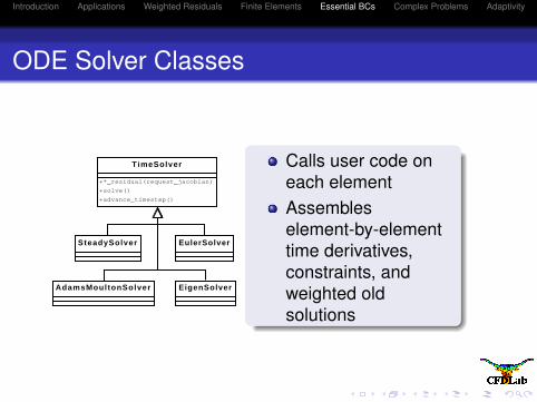
ODE Solver Classes
TimeSolver
+*_residual(request_jacobian)
+solve()
+advance_timestep()
SteadySolver EulerSolver
AdamsMoultonSolver EigenSolver
Calls user code oneach elementAssembleselement-by-elementtime derivatives,constraints, andweighted oldsolutions

Introduction Applications Weighted Residuals Finite Elements Essential BCs Complex Problems Adaptivity
Nonlinear Solver Classes
NonlinearSolver
+*_tolerance
+*_max_iterations
+solve()
QuasiNewtonSolverLinearSolver
ContinuationSolver
Acquires residuals,jacobians from ODEsolverHandles inner loops,inner solvers andtolerances,convergence tests,etc
Introduction Applications Weighted Residuals Finite Elements Essential BCs Complex Problems Adaptivity
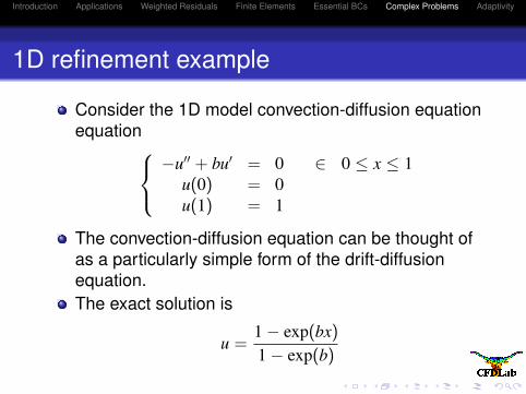
1D refinement example
Consider the 1D model convection-diffusion equationequation
−u′′ + bu′ = 0 ∈ 0 ≤ x ≤ 1u(0) = 0u(1) = 1
The convection-diffusion equation can be thought ofas a particularly simple form of the drift-diffusionequation.The exact solution is
u =1− exp(bx)1− exp(b)
Introduction Applications Weighted Residuals Finite Elements Essential BCs Complex Problems Adaptivity
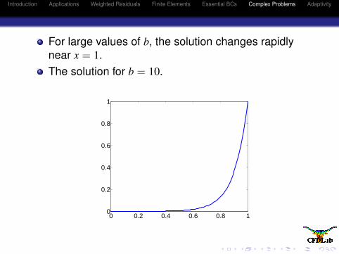
For large values of b, the solution changes rapidlynear x = 1.The solution for b = 10.
0 0.2 0.4 0.6 0.8 10
0.2
0.4
0.6
0.8
1
Introduction Applications Weighted Residuals Finite Elements Essential BCs Complex Problems Adaptivity
We assume here that we have an approximatesolution uh which is the linear interpolant of u.We will measure the error between the exact solutionu and the approximate solution uh in the following (L2)norm:
‖e‖2L2
:= ‖u− uh‖2L2
=
∫ 1
0(u− uh)
2 dx
Consider a sequence of uniformly-refined meshes . . .
Introduction Applications Weighted Residuals Finite Elements Essential BCs Complex Problems Adaptivity
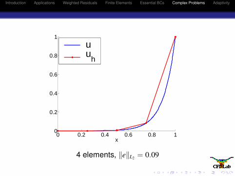
0 0.2 0.4 0.6 0.8 10
0.2
0.4
0.6
0.8
1
x
uu
h
4 elements, ‖e‖L2 = 0.09
Introduction Applications Weighted Residuals Finite Elements Essential BCs Complex Problems Adaptivity
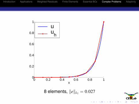
0 0.2 0.4 0.6 0.8 10
0.2
0.4
0.6
0.8
1
x
uu
h
8 elements, ‖e‖L2 = 0.027
Introduction Applications Weighted Residuals Finite Elements Essential BCs Complex Problems Adaptivity
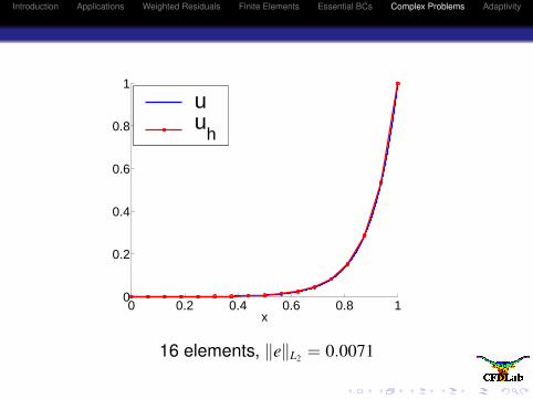
0 0.2 0.4 0.6 0.8 10
0.2
0.4
0.6
0.8
1
x
uu
h
16 elements, ‖e‖L2 = 0.0071
Introduction Applications Weighted Residuals Finite Elements Essential BCs Complex Problems Adaptivity
Adaptive Refinement
Q: Can we do “better” than uniform refinement?A: Yes, if we refine cells which have higher errorrelative to others.
Introduction Applications Weighted Residuals Finite Elements Essential BCs Complex Problems Adaptivity
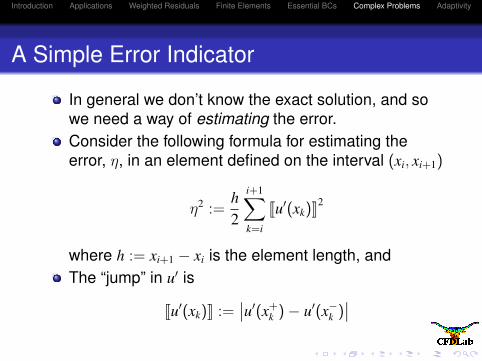
A Simple Error Indicator
In general we don’t know the exact solution, and sowe need a way of estimating the error.Consider the following formula for estimating theerror, η, in an element defined on the interval (xi, xi+1)
η2 :=h2
i+1∑k=i
Ju′(xk)K2
where h := xi+1 − xi is the element length, andThe “jump” in u′ is
Ju′(xk)K :=∣∣u′(x+
k )− u′(x−k )∣∣
Introduction Applications Weighted Residuals Finite Elements Essential BCs Complex Problems Adaptivity
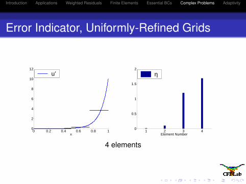
Error Indicator, Uniformly-Refined Grids
0 0.2 0.4 0.6 0.8 10
2
4
6
8
10
12
x
u’
1 2 3 40
0.5
1
1.5
2
Element Number
η
4 elements
Introduction Applications Weighted Residuals Finite Elements Essential BCs Complex Problems Adaptivity
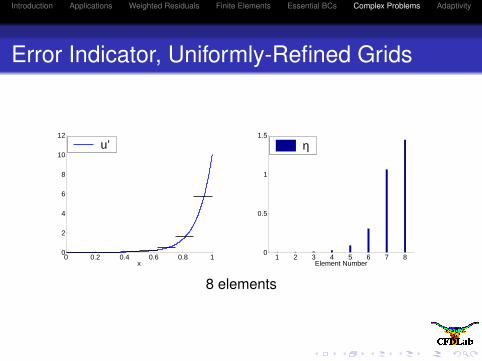
Error Indicator, Uniformly-Refined Grids
0 0.2 0.4 0.6 0.8 10
2
4
6
8
10
12
x
u’
1 2 3 4 5 6 7 80
0.5
1
1.5
Element Number
η
8 elements
Introduction Applications Weighted Residuals Finite Elements Essential BCs Complex Problems Adaptivity
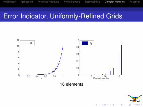
Error Indicator, Uniformly-Refined Grids
0 0.2 0.4 0.6 0.8 10
2
4
6
8
10
12
x
u’
5 10 150
0.2
0.4
0.6
0.8
1
Element Number
η
16 elements
Introduction Applications Weighted Residuals Finite Elements Essential BCs Complex Problems Adaptivity
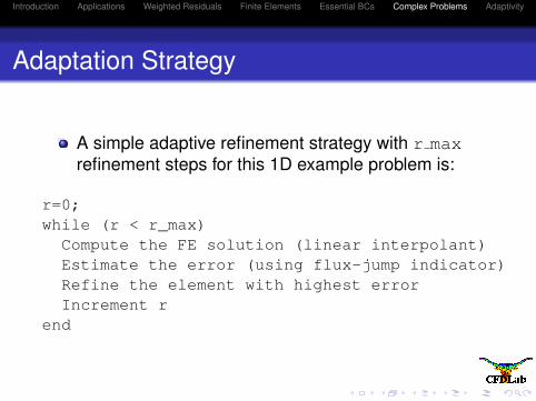
Adaptation Strategy
A simple adaptive refinement strategy with r maxrefinement steps for this 1D example problem is:
r=0;while (r < r_max)Compute the FE solution (linear interpolant)Estimate the error (using flux-jump indicator)Refine the element with highest errorIncrement r
end
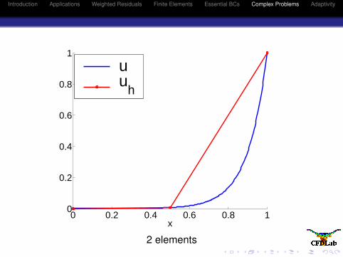
Introduction Applications Weighted Residuals Finite Elements Essential BCs Complex Problems Adaptivity
0 0.2 0.4 0.6 0.8 10
0.2
0.4
0.6
0.8
1
x
uu
h
2 elements
Introduction Applications Weighted Residuals Finite Elements Essential BCs Complex Problems Adaptivity
0 0.2 0.4 0.6 0.8 10
0.2
0.4
0.6
0.8
1
x
uu
h
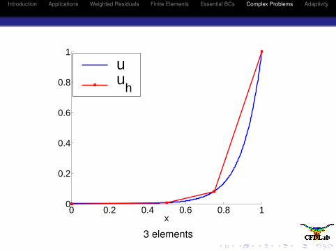
3 elements
Introduction Applications Weighted Residuals Finite Elements Essential BCs Complex Problems Adaptivity
0 0.2 0.4 0.6 0.8 10
0.2
0.4
0.6
0.8
1
x
uu
h
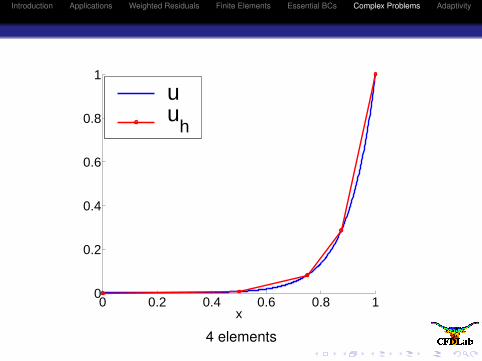
4 elements

Introduction Applications Weighted Residuals Finite Elements Essential BCs Complex Problems Adaptivity
0 0.2 0.4 0.6 0.8 10
0.2
0.4
0.6
0.8
1
x
uu
h
5 elements
Introduction Applications Weighted Residuals Finite Elements Essential BCs Complex Problems Adaptivity
0 0.2 0.4 0.6 0.8 10
0.2
0.4
0.6
0.8
1
x
uu
h
6 elements

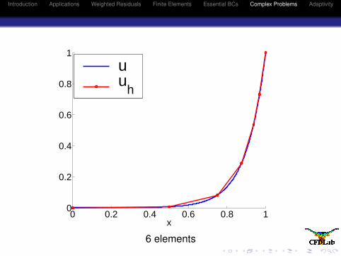
Introduction Applications Weighted Residuals Finite Elements Essential BCs Complex Problems Adaptivity
0 0.2 0.4 0.6 0.8 10
0.2
0.4
0.6
0.8
1
x
uu
h
7 elements

Introduction Applications Weighted Residuals Finite Elements Essential BCs Complex Problems Adaptivity
0 0.2 0.4 0.6 0.8 10
0.2
0.4
0.6
0.8
1
x
uu
h
8 elements

Introduction Applications Weighted Residuals Finite Elements Essential BCs Complex Problems Adaptivity
0 0.2 0.4 0.6 0.8 10
0.2
0.4
0.6
0.8
1
x
uu
h
9 elements
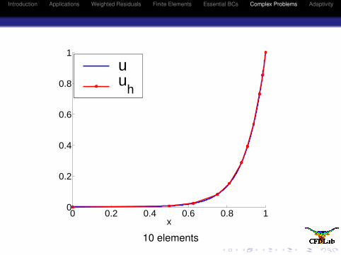
Introduction Applications Weighted Residuals Finite Elements Essential BCs Complex Problems Adaptivity
0 0.2 0.4 0.6 0.8 10
0.2
0.4
0.6
0.8
1
x
uu
h
10 elements
Introduction Applications Weighted Residuals Finite Elements Essential BCs Complex Problems Adaptivity
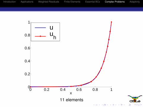
0 0.2 0.4 0.6 0.8 10
0.2
0.4
0.6
0.8
1
x
uu
h
11 elements
Introduction Applications Weighted Residuals Finite Elements Essential BCs Complex Problems Adaptivity
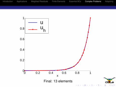
0 0.2 0.4 0.6 0.8 10
0.2
0.4
0.6
0.8
1
x
uu
h
Final: 13 elements
Introduction Applications Weighted Residuals Finite Elements Essential BCs Complex Problems Adaptivity
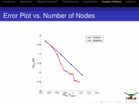
Error Plot vs. Number of Nodes
0.2 0.4 0.6 0.8 1 1.2 1.4 1.6−3
−2.5
−2
−1.5
−1
−0.5
0
log10
Nnodes
log 10
||e|
|
UniformAdaptive
Introduction Applications Weighted Residuals Finite Elements Essential BCs Complex Problems Adaptivity
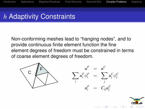
h Adaptivity Constraints
Non-conforming meshes lead to “hanging nodes”, and toprovide continuous finite element function the fineelement degrees of freedom must be constrained in termsof coarse element degrees of freedom.
FC
uF = uC∑i
uFi φF
i =∑
j
uCj φC
j
uFi = CijuC
j
Introduction Applications Weighted Residuals Finite Elements Essential BCs Complex Problems Adaptivity
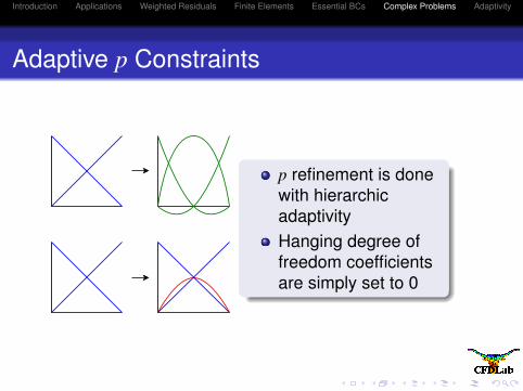
Adaptive p Constraints
p refinement is donewith hierarchicadaptivityHanging degree offreedom coefficientsare simply set to 0
Introduction Applications Weighted Residuals Finite Elements Essential BCs Complex Problems Adaptivity
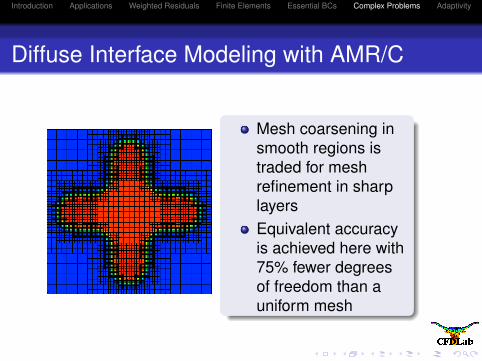
Diffuse Interface Modeling with AMR/C
Mesh coarsening insmooth regions istraded for meshrefinement in sharplayersEquivalent accuracyis achieved here with75% fewer degreesof freedom than auniform mesh

Introduction Applications Weighted Residuals Finite Elements Essential BCs Complex Problems Adaptivity
Installing libMesh
PETSc Download, Installation instructions,Documentation:http://www-unix.mcs.anl.gov/petsc/petsc-2/
libMesh Downloads, Installation instructions,Documentation:http://libmesh.sourceforge.net/
Introduction Applications Weighted Residuals Finite Elements Essential BCs Complex Problems Adaptivity
Reference
B. Kirk, J. Peterson, R. Stogner and G. Carey,“libMesh: a C++ library for parallel adaptive meshrefinement/coarsening simulations”, Engineering withComputers, in press.