lidar report - enecafe.com
TRANSCRIPT
Measurements of Wind Profile from a Buoy using Lidar
Final Report
Report prepared by CMR, University of Bergen, Statoil, Marintek and Fugro OCEANOR
Reference No: 9631
5 June 2012

II 9631/R0/05-06-2012
TABLE OF CONTENTS
1. Introduction .......................................................................................................................1
2. Review of the Tasks..........................................................................................................2
2.1 Formulation of requirement and specification of the system ..................................2
2.2 Concept Study ........................................................................................................2
2.2.1 Lidar motion test ......................................................................................2
2.2.2 Hydrodynamic simulations ......................................................................6
2.2.3 The motion compensation algorithm .......................................................7
3. Description of the measurement system.........................................................................10
3.1 The Wavescan buoy .............................................................................................10
3.2 The ZephIR lidar ...................................................................................................11
3.3 The buoy system...................................................................................................12
4. Field test..........................................................................................................................14

1 9631/R0/05-06-2012
1. Introduction
The interest for offshore wind farms is increasing due to increased demand of energy world wide and that
climate change has increased the interest for renewable energy.
Reliable data of the wind profile for the relevant height of recent and future wind generators (30-300m)
are important both for design, estimation of wind energy potential and during operations. As the power
production of wind turbines increases with the 3rd
power of the wind speed, accurate measurements of
the wind profile is important both with respect to financing and profitability of the investments. Up to now
such measurements have been carried out on bottom met mast which is expensive and stationary. By
measuring the measurements from a portable buoy the cost will be decreased by a factor 10 or more.
The objective of this project was to develop and demonstrate the feasibility of an autonomous system for
measuring wind profile, waves and current profile from an anchored floating buoy.
The system should be able to measure wind profile in the region from 30-300 meters above sea level,
relevant for actual and future offshore wind farms. Applications for such a measurement system include:
• Mapping of wind potential (main focus in this project)
• Optimisation of wind farm during operation (not main focus in this project)
• Determination of structural loads and expected fatigue
• Validation of numerical simulations of the atmospheric and oceanic boundary layer
• Measurement of wake effect (not main focus in this project)
The project included the following tasks:
1. Formulation of requirement and specification of the system
2. Concept study
3. Development of a prototype including hydrodynamic simulations
4. Development of a compensation algorithm for the buoy motion
5. Building of a prototype buoy
6. Field test of the buoy
The following institutions participated in the project: Fugro OCEANOR, Statoil, University of Bergen,
Christian Michelsen Research (CMR) and Marintek.
2 9631/R0/05-06-2012
2. Review of the Tasks
2.1 Formulation of requirement and specification of the system
In this task the following requirements were specified:
• Measurement parameters
• The wind profile sensor
• The measurement platform
• Support system such as power supply, mooring and communication system
• Operation and maintenance
Reports
Specification of a Buoy System for measuring Wind Profile. Report prepared by CMR, University of
Bergen, Statoil, Marintek and Fugro OCEANOR.
2.2 Concept Study
This task included the following activities:
• Evaluation of concept for wind profiling
• Lidar motion test
• Hydrodynamic simulation
A literature study was carried out by CMR reviewing existing technologies such as sodar, radar and lidar
for remote wind measurements. Combined solutions such as Radio Acoustic Sounding System (RASS)
were also evaluated. Option for local wind measurement to be used on the buoy was also covered. Lidar
was perceived to be the best technology based on benefits especially related to size, accuracy and power
requirements. Lidar systems come in two main classes, continuous wave (CW) or pulsed, both with its
strengths and weaknesses. The evaluation recommended testing both options further with respect to
capability of working acceptable on a moving platform. The results from a comparison test performed as
part of this project are covered in section 2.2.1 below.
Report:
CMR-10-F10255-RA-1 Concept for wind profiling for offshore wind energy applications. Report prepared
by CMR and the University in Bergen.
2.2.1 Lidar motion test
To examining the influence of wave motion on the lidar wind profile measurements, a motion test was
carried out at the University of Agder, Grimstad autumn 2011. A motion platform was rented free of
charge from the University in Agder, campus Grimstad, as this infrastructure was funded by NORCOWE.
A motion sensor and sonic anemometer was also rented free of charge from NORCOWE. The motion
platform used had 6 degrees of freedom, with the possibility of controlling frequency and amplitude
individually. The motions along the following principal axis; roll, pitch, yaw, heave and surge, in addition to
3 9631/R0/05-06-2012
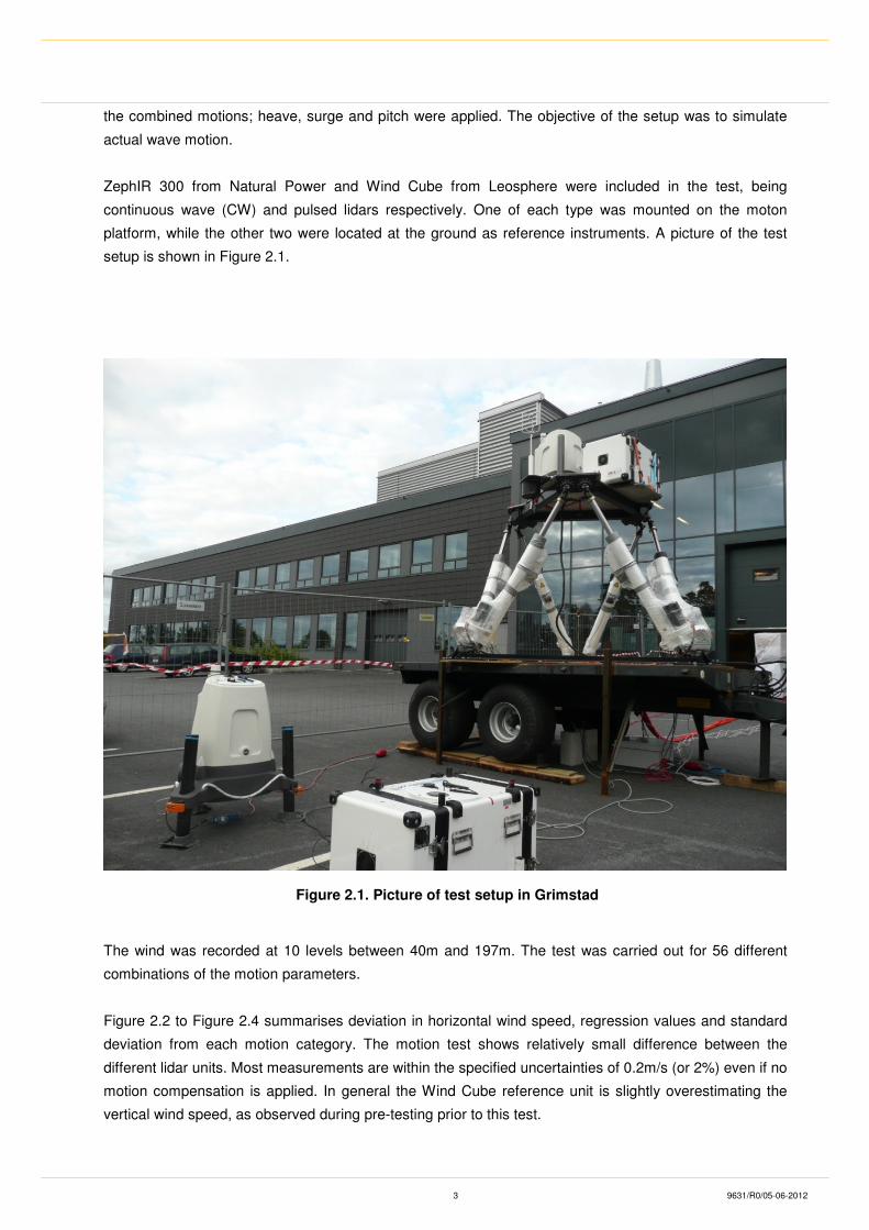
the combined motions; heave, surge and pitch were applied. The objective of the setup was to simulate
actual wave motion.
ZephIR 300 from Natural Power and Wind Cube from Leosphere were included in the test, being
continuous wave (CW) and pulsed lidars respectively. One of each type was mounted on the moton
platform, while the other two were located at the ground as reference instruments. A picture of the test
setup is shown in Figure 2.1.
Figure 2.1. Picture of test setup in Grimstad
The wind was recorded at 10 levels between 40m and 197m. The test was carried out for 56 different
combinations of the motion parameters.
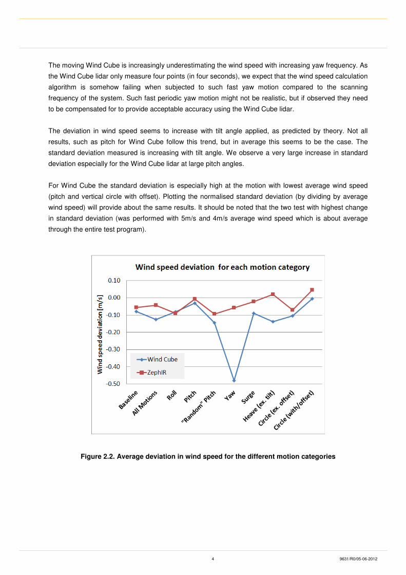
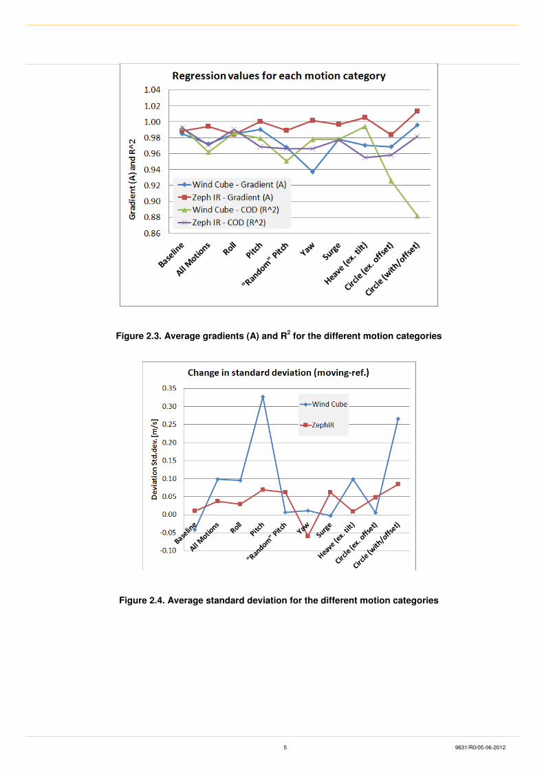
Figure 2.2 to Figure 2.4 summarises deviation in horizontal wind speed, regression values and standard
deviation from each motion category. The motion test shows relatively small difference between the
different lidar units. Most measurements are within the specified uncertainties of 0.2m/s (or 2%) even if no
motion compensation is applied. In general the Wind Cube reference unit is slightly overestimating the
vertical wind speed, as observed during pre-testing prior to this test.
4 9631/R0/05-06-2012
The moving Wind Cube is increasingly underestimating the wind speed with increasing yaw frequency. As
the Wind Cube lidar only measure four points (in four seconds), we expect that the wind speed calculation
algorithm is somehow failing when subjected to such fast yaw motion compared to the scanning
frequency of the system. Such fast periodic yaw motion might not be realistic, but if observed they need
to be compensated for to provide acceptable accuracy using the Wind Cube lidar.
The deviation in wind speed seems to increase with tilt angle applied, as predicted by theory. Not all
results, such as pitch for Wind Cube follow this trend, but in average this seems to be the case. The
standard deviation measured is increasing with tilt angle. We observe a very large increase in standard
deviation especially for the Wind Cube lidar at large pitch angles.
For Wind Cube the standard deviation is especially high at the motion with lowest average wind speed
(pitch and vertical circle with offset). Plotting the normalised standard deviation (by dividing by average
wind speed) will provide about the same results. It should be noted that the two test with highest change
in standard deviation (was performed with 5m/s and 4m/s average wind speed which is about average
through the entire test program).
Figure 2.2. Average deviation in wind speed for the different motion categories
5 9631/R0/05-06-2012
Figure 2.3. Average gradients (A) and R2 for the different motion categories
Figure 2.4. Average standard deviation for the different motion categories
6 9631/R0/05-06-2012
Report: CMR-11-F10255-RA-1 Lidar Motion Test, Grimstad 2011 – Setup and results
Web article: www.forskning.no Laser høy sjø (http://www.forskning.no/artikler/2012/mars/315770)
Presentation: “Effect of wave motion on wind lidar measurements - Comparison
(http://www.wire1002.ch/)
We are also writing on a peer review paper planned submitted to the journal Wind Energy.
The lidar comparison test was performed by CMR with support from the University in Bergen. We also
like to take this opportunity to thank the staff at the University in Agder for their support enabling this test.
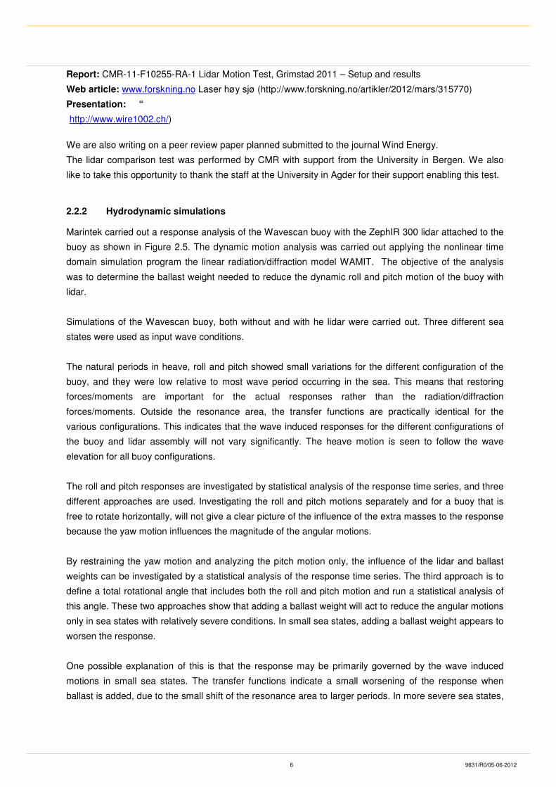
2.2.2 Hydrodynamic simulations
Marintek carried out a response analysis of the Wavescan buoy with the ZephIR 300 lidar attached to the
buoy as shown in Figure 2.5. The dynamic motion analysis was carried out applying the nonlinear time
domain simulation program the linear radiation/diffraction model WAMIT. The objective of the analysis
was to determine the ballast weight needed to reduce the dynamic roll and pitch motion of the buoy with
lidar.
Simulations of the Wavescan buoy, both without and with he lidar were carried out. Three different sea
states were used as input wave conditions.
The natural periods in heave, roll and pitch showed small variations for the different configuration of the
buoy, and they were low relative to most wave period occurring in the sea. This means that restoring
forces/moments are important for the actual responses rather than the radiation/diffraction
forces/moments. Outside the resonance area, the transfer functions are practically identical for the
various configurations. This indicates that the wave induced responses for the different configurations of
the buoy and lidar assembly will not vary significantly. The heave motion is seen to follow the wave
elevation for all buoy configurations.
The roll and pitch responses are investigated by statistical analysis of the response time series, and three
different approaches are used. Investigating the roll and pitch motions separately and for a buoy that is
free to rotate horizontally, will not give a clear picture of the influence of the extra masses to the response
because the yaw motion influences the magnitude of the angular motions.
By restraining the yaw motion and analyzing the pitch motion only, the influence of the lidar and ballast
weights can be investigated by a statistical analysis of the response time series. The third approach is to
define a total rotational angle that includes both the roll and pitch motion and run a statistical analysis of
this angle. These two approaches show that adding a ballast weight will act to reduce the angular motions
only in sea states with relatively severe conditions. In small sea states, adding a ballast weight appears to
worsen the response.
One possible explanation of this is that the response may be primarily governed by the wave induced
motions in small sea states. The transfer functions indicate a small worsening of the response when
ballast is added, due to the small shift of the resonance area to larger periods. In more severe sea states,
7 9631/R0/05-06-2012
the wind and current forces seem to become increasingly important for the response, and it is possible
that the ballast weight counteracts these forces/moments, yielding a small reduction in the response.
Report
Development of Wavescan Buoy with Lidar-Motion analysis. Marintek report October 2011.
Figure 2.5. The configuration of the Wavescan buoy and the lidar used in the simulations.
2.2.3 The motion compensation algorithm
The compensation algorithm for motion corrections has been developed by Uni Computing, University of
Bergen. The algorithm can use all the 6 degree of freedom data measured by the wave sensor in the
8 9631/R0/05-06-2012
buoy, to compensate the lidar wind measurements for the buoy motion. The algorithm uses the 1 sec
data from the Wave sensor to compensate the 1 sec wind measurements at each height.
Principle behind motion compensation algorithm
The algorithm used is based on that employed by Edson et al. (1998). Given a velocity vector
uo
measured with respect to a coordinate system (x, y, zo
) which is fixed with reference to an instrument
platform, we obtain the velocity with respect to a reference (“true”) coordinate system (x, y, z) by means
of the following transformation:
u = T(uo
+ ΩΩΩΩ × R) + Vmot
where
u is the ‘true' velocity, uo
is the observed velocity, Ωo
is the angular velocity vector of the motion package,
R is the position vector of the sensor with respect to the motion package which senses the linear and
angular movement of the instrument platform, V t
is the velocity of the motion package with respect to the
reference coordinate system, and T is the rotational transformation matrix between the platform
coordinate system and the reference coordinates.
Testing of motion compensation algorithm
Lidar motion test at Grimstad
The motion compensation algorithm was applied for the WindCube lidar, as 1-second data for the
individual beams are available. For the ZephIR lidar, the individual beam information was not available,
and an alternative algorithm based on the integrated 1-second data for the 360 degree scan needs to be
used (algorithm under development).
The compensation algorithm was applied for the individual test runs 003 (heave 40 cm), 006 (Surge N-S
40cm), 010 (tilt N-S 10 degrees 0.2Hz), 014 (vertical circle 30cm), 011 (Tilt N-S 15 degrees), and 047
(strong gale max 17 degrees tilt).
Field test
The motion compensation algorithm is now being tested using data from the field test at Titran.
9 9631/R0/05-06-2012
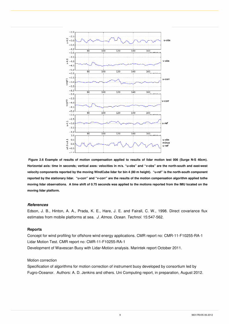
Figure 2.6 Example of results of motion compensation applied to results of lidar motion test 006 (Surge N-S 40cm).
Horizontal axis: time in seconds; vertical axes: velocities in m/s. “u-obs” and “v-obs” are the north-south and east-west
velocity components reported by the moving WindCube lidar for bin 4 (80 m height). “u-ref” is the north-south component
reported by the stationary lidar. “u-corr” and “v-corr” are the results of the motion compensation algorithm applied tothe
moving lidar observations. A time shift of 0.75 seconds was applied to the motions reported from the IMU located on the
moving lidar platform.
References
Edson, J. B., Hinton, A. A., Prada, K. E., Hare, J. E. and Fairall, C. W., 1998. Direct covariance flux
estimates from mobile platforms at sea. J. Atmos. Ocean. Technol. 15:547-562.
Reports
Concept for wind profiling for offshore wind energy applications. CMR report no: CMR-11-F10255-RA-1
Lidar Motion Test. CMR report no: CMR-11-F10255-RA-1
Development of Wavescan Buoy with Lidar-Motion analysis. Marintek report October 2011.
Motion correction
Specification of algorithms for motion correction of instrument buoy developed by consortium led by
Fugro-Oceanor. Authors: A. D. Jenkins and others. Uni Computing report, in preparation, August 2012.
10 9631/R0/05-06-2012
3. Description of the measurement system
The Wavescan Lidar buoy includes a ZephIR 300 lidar attached to the Wavescan buoy. Below is given a
description of the different elements and the ant the assembling of the system.
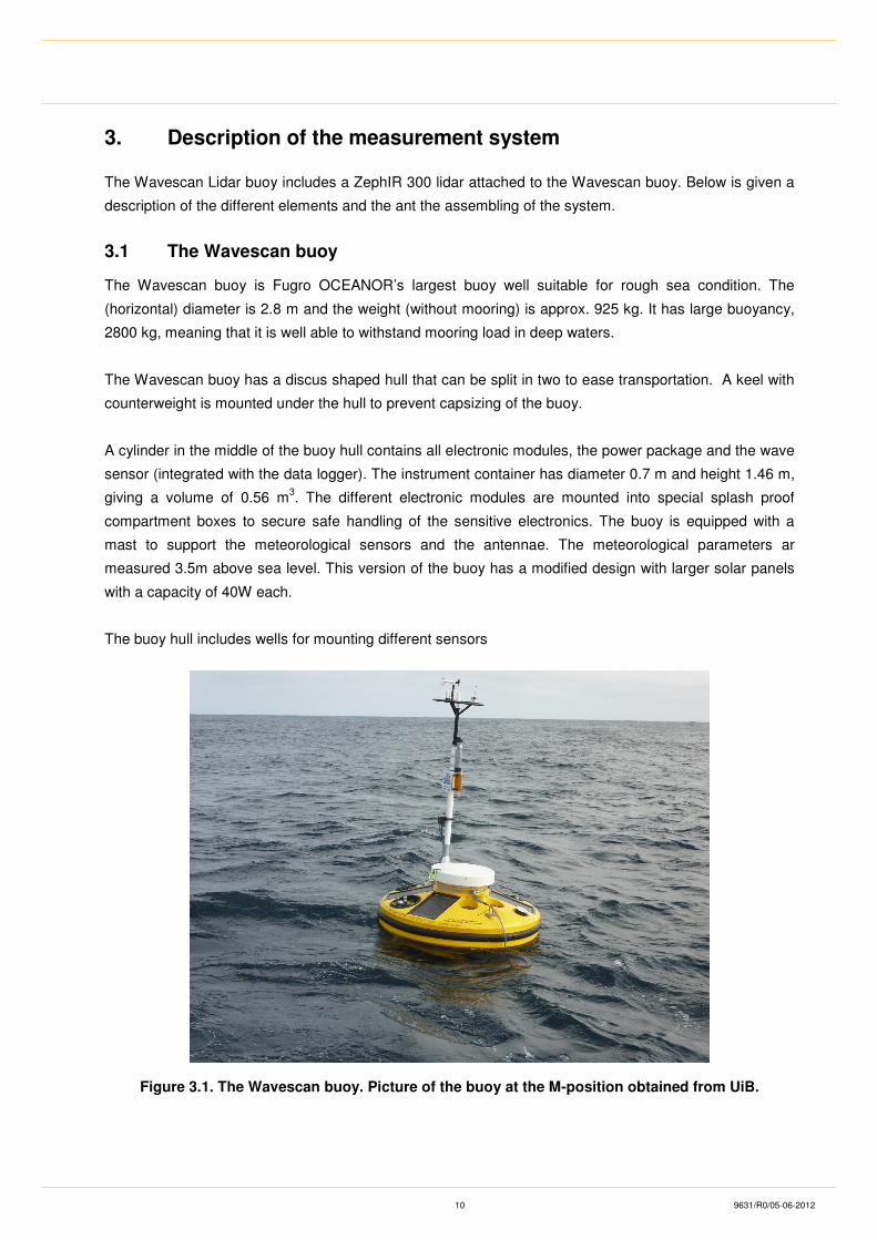
3.1 The Wavescan buoy
The Wavescan buoy is Fugro OCEANOR’s largest buoy well suitable for rough sea condition. The
(horizontal) diameter is 2.8 m and the weight (without mooring) is approx. 925 kg. It has large buoyancy,
2800 kg, meaning that it is well able to withstand mooring load in deep waters.
The Wavescan buoy has a discus shaped hull that can be split in two to ease transportation. A keel with
counterweight is mounted under the hull to prevent capsizing of the buoy.
A cylinder in the middle of the buoy hull contains all electronic modules, the power package and the wave
sensor (integrated with the data logger). The instrument container has diameter 0.7 m and height 1.46 m,
giving a volume of 0.56 m3. The different electronic modules are mounted into special splash proof
compartment boxes to secure safe handling of the sensitive electronics. The buoy is equipped with a
mast to support the meteorological sensors and the antennae. The meteorological parameters ar
measured 3.5m above sea level. This version of the buoy has a modified design with larger solar panels
with a capacity of 40W each.
The buoy hull includes wells for mounting different sensors
Figure 3.1. The Wavescan buoy. Picture of the buoy at the M-position obtained from UiB.
11 9631/R0/05-06-2012
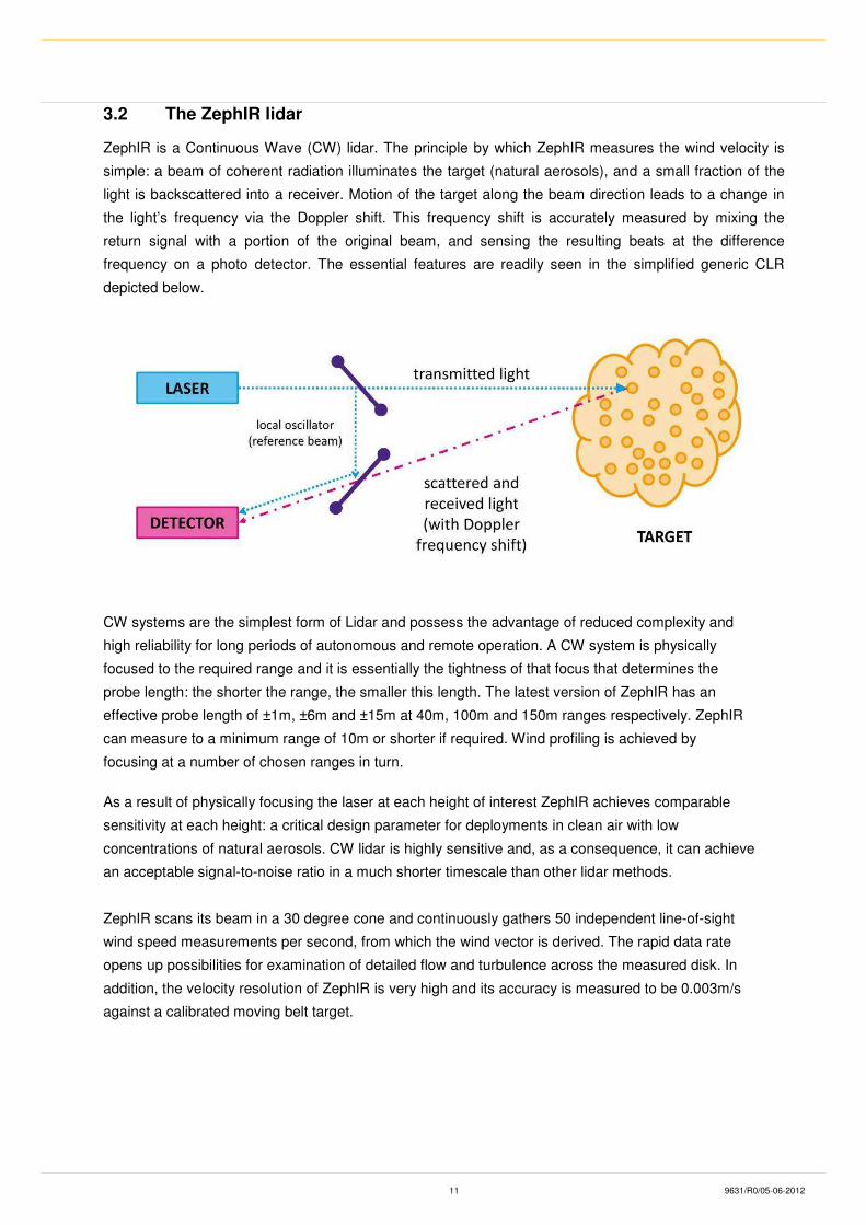
3.2 The ZephIR lidar
ZephIR is a Continuous Wave (CW) lidar. The principle by which ZephIR measures the wind velocity is
simple: a beam of coherent radiation illuminates the target (natural aerosols), and a small fraction of the
light is backscattered into a receiver. Motion of the target along the beam direction leads to a change in
the light’s frequency via the Doppler shift. This frequency shift is accurately measured by mixing the
return signal with a portion of the original beam, and sensing the resulting beats at the difference
frequency on a photo detector. The essential features are readily seen in the simplified generic CLR
depicted below.
CW systems are the simplest form of Lidar and possess the advantage of reduced complexity and
high reliability for long periods of autonomous and remote operation. A CW system is physically
focused to the required range and it is essentially the tightness of that focus that determines the
probe length: the shorter the range, the smaller this length. The latest version of ZephIR has an
effective probe length of ±1m, ±6m and ±15m at 40m, 100m and 150m ranges respectively. ZephIR
can measure to a minimum range of 10m or shorter if required. Wind profiling is achieved by
focusing at a number of chosen ranges in turn.
As a result of physically focusing the laser at each height of interest ZephIR achieves comparable
sensitivity at each height: a critical design parameter for deployments in clean air with low
concentrations of natural aerosols. CW lidar is highly sensitive and, as a consequence, it can achieve
an acceptable signal-to-noise ratio in a much shorter timescale than other lidar methods.
ZephIR scans its beam in a 30 degree cone and continuously gathers 50 independent line-of-sight
wind speed measurements per second, from which the wind vector is derived. The rapid data rate
opens up possibilities for examination of detailed flow and turbulence across the measured disk. In
addition, the velocity resolution of ZephIR is very high and its accuracy is measured to be 0.003m/s
against a calibrated moving belt target.
12 9631/R0/05-06-2012
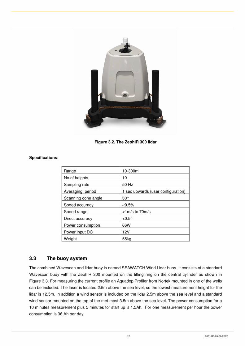
Figure 3.2. The ZephIR 300 lidar
Specifications:
Range 10-300m
No of heights 10
Sampling rate 50 Hz
Averaging period 1 sec upwards (user configuration)
Scanning cone angle 30°
Speed accuracy <0.5%
Speed range <1m/s to 70m/s
Direct accuracy <0.5°
Power consumption 66W
Power input DC 12V
Weight 55kg
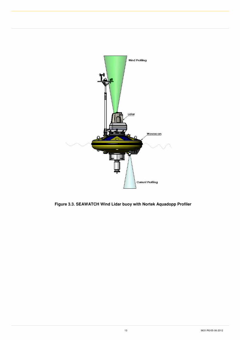
3.3 The buoy system
The combined Wavescan and lidar buoy is named SEAWATCH Wind Lidar buoy. It consists of a standard
Wavescan buoy with the ZephIR 300 mounted on the lifting ring on the central cylinder as shown in
Figure 3.3. For measuring the current profile an Aquadop Profiler from Nortek mounted in one of the wells
can be included. The laser is located 2.5m above the sea level, so the lowest measurement height for the
lidar is 12.5m. In addition a wind sensor is included on the lidar 2.5m above the sea level and a standard
wind sensor mounted on the top of the met mast 3.5m above the sea level. The power consumption for a
10 minutes measurement plus 5 minutes for start up is 1.5Ah. For one measurement per hour the power
consumption is 36 Ah per day.
13 9631/R0/05-06-2012
Figure 3.3. SEAWATCH Wind Lidar buoy with Nortek Aquadopp Profiler
14 9631/R0/05-06-2012
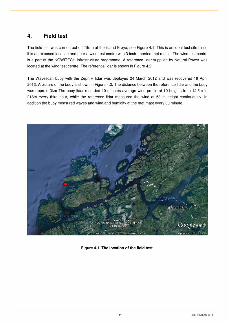
4. Field test
The field test was carried out off Titran at the island Frøya, see Figure 4.1. This is an ideal test site since
it is an exposed location and near a wind test centre with 3 instrumented met masts. The wind test centre
is a part of the NOWITECH infrastructure programme. A reference lidar supplied by Natural Power was
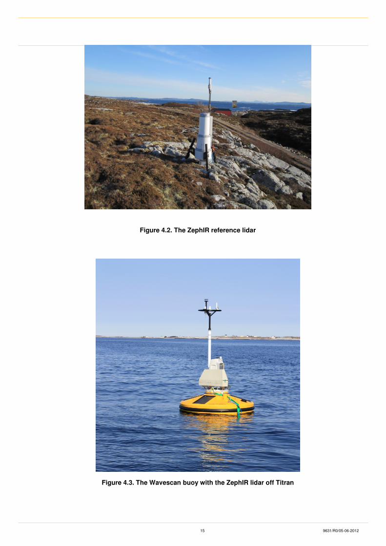
located at the wind test centre. The reference lidar is shown in Figure 4.2.
The Wavescan buoy with the ZephIR lidar was deployed 24 March 2012 and was recovered 19 April
2012. A picture of the buoy is shown in Figure 4.3. The distance between the reference lidar and the buoy
was approx. 3km The buoy lidar recorded 10 minutes average wind profile at 10 heights from 12.5m to
218m every third hour, while the reference lidar measured the wind at 53 m height continuously. In
addition the buoy measured waves and wind and humidity at the met mast every 30 minute.
Figure 4.1. The location of the field test.
15 9631/R0/05-06-2012
Figure 4.2. The ZephIR reference lidar
Figure 4.3. The Wavescan buoy with the ZephIR lidar off Titran
16 9631/R0/05-06-2012
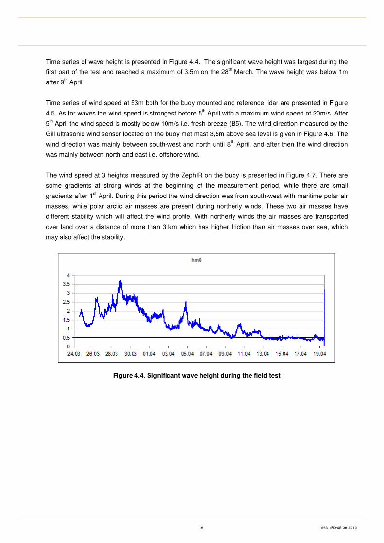
Time series of wave height is presented in Figure 4.4. The significant wave height was largest during the
first part of the test and reached a maximum of 3.5m on the 28th March. The wave height was below 1m
after 9th April.
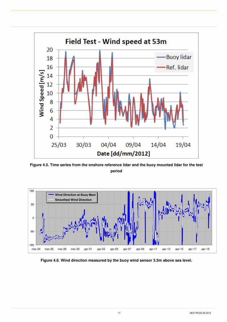
Time series of wind speed at 53m both for the buoy mounted and reference lidar are presented in Figure
4.5. As for waves the wind speed is strongest before 5th April with a maximum wind speed of 20m/s. After
5th April the wind speed is mostly below 10m/s i.e. fresh breeze (B5). The wind direction measured by the
Gill ultrasonic wind sensor located on the buoy met mast 3,5m above sea level is given in Figure 4.6. The
wind direction was mainly between south-west and north until 8th April, and after then the wind direction
was mainly between north and east i.e. offshore wind.
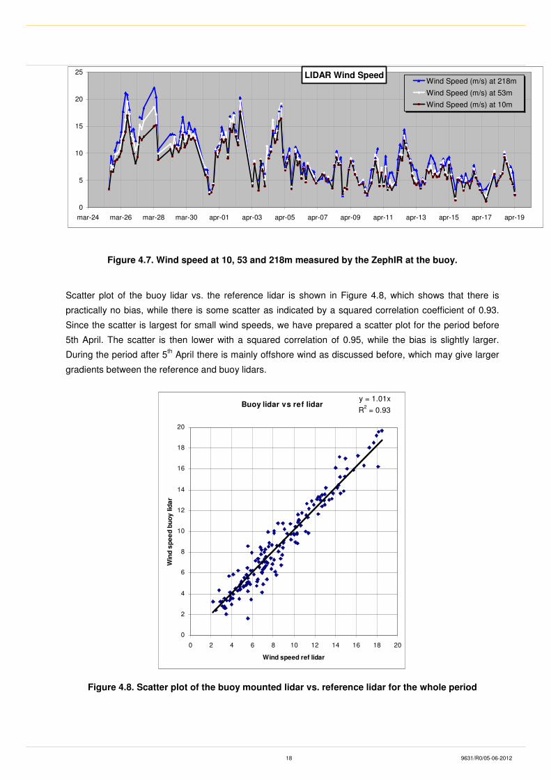
The wind speed at 3 heights measured by the ZephIR on the buoy is presented in Figure 4.7. There are
some gradients at strong winds at the beginning of the measurement period, while there are small
gradients after 1st April. During this period the wind direction was from south-west with maritime polar air
masses, while polar arctic air masses are present during northerly winds. These two air masses have
different stability which will affect the wind profile. With northerly winds the air masses are transported
over land over a distance of more than 3 km which has higher friction than air masses over sea, which
may also affect the stability.
Figure 4.4. Significant wave height during the field test
17 9631/R0/05-06-2012
Figure 4.5. Time series from the onshore reference lidar and the buoy mounted lidar for the test
period
-180
-90
0
90
180
mar-24 mar-26 mar-28 mar-30 apr-01 apr-03 apr-05 apr-07 apr-09 apr-11 apr-13 apr-15 apr-17 apr-19
Wind Direction at Buoy Mast
Smoothed Wind Direction
Figure 4.6. Wind direction measured by the buoy wind sensor 3.5m above sea level.
18 9631/R0/05-06-2012
LIDAR Wind Speed
0
5
10
15
20
25
mar-24 mar-26 mar-28 mar-30 apr-01 apr-03 apr-05 apr-07 apr-09 apr-11 apr-13 apr-15 apr-17 apr-19
Wind Speed (m/s) at 218m
Wind Speed (m/s) at 53m
Wind Speed (m/s) at 10m
Figure 4.7. Wind speed at 10, 53 and 218m measured by the ZephIR at the buoy.
Scatter plot of the buoy lidar vs. the reference lidar is shown in Figure 4.8, which shows that there is
practically no bias, while there is some scatter as indicated by a squared correlation coefficient of 0.93.
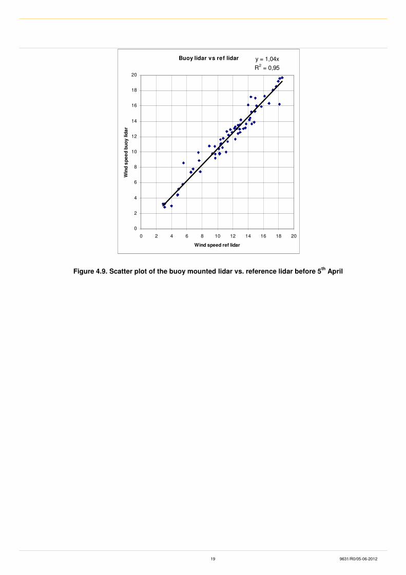
Since the scatter is largest for small wind speeds, we have prepared a scatter plot for the period before
5th April. The scatter is then lower with a squared correlation of 0.95, while the bias is slightly larger.
During the period after 5th April there is mainly offshore wind as discussed before, which may give larger
gradients between the reference and buoy lidars.
Buoy lidar vs ref lidary = 1.01x
R2 = 0.93
0
2
4
6
8
10
12
14
16
18
20
0 2 4 6 8 10 12 14 16 18 20
Wind speed ref lidar
Win
d s
pe
ed
bu
oy
lid
ar
Figure 4.8. Scatter plot of the buoy mounted lidar vs. reference lidar for the whole period
19 9631/R0/05-06-2012
Buoy lidar vs ref lidar y = 1,04x
R2 = 0,95
0
2
4
6
8
10
12
14
16
18
20
0 2 4 6 8 10 12 14 16 18 20
Wind speed ref lidar
Win
d s
pe
ed
bu
oy
lid
ar
Figure 4.9. Scatter plot of the buoy mounted lidar vs. reference lidar before 5th
April