HAL Id: hal-00001155https://hal.archives-ouvertes.fr/hal-00001155v2

Submitted on 1 Mar 2004

HAL is a multi-disciplinary open accessarchive for the deposit and dissemination of sci-entific research documents, whether they are pub-lished or not. The documents may come fromteaching and research institutions in France orabroad, or from public or private research centers.

L’archive ouverte pluridisciplinaire HAL, estdestinée au dépôt et à la diffusion de documentsscientifiques de niveau recherche, publiés ou non,émanant des établissements d’enseignement et derecherche français ou étrangers, des laboratoirespublics ou privés.

Lie Groups and mechanics: an introductionBoris Kolev

To cite this version:Boris Kolev. Lie Groups and mechanics: an introduction. Adrian Constantin and Joachim Escher.Wave motion, Jan 2004, Oberwolfach, Germany. Journal of Nonlinear Mathematical Physics, 11 (4),pp.480-498, 2004, Volume 11. <10.2991/jnmp.2004.11.4.5>. <hal-00001155v2>

ccsd

-000

0115

5 (v

ersi

on 2

) : 1

Mar

200

4

LIE GROUPS AND MECHANICS,

AN INTRODUCTION

BORIS KOLEV

Abstract. The aim of this paper is to present aspects of the use of Liegroups in mechanics. We start with the motion of the rigid body forwhich the main concepts are extracted. In a second part, we extend thetheory for an arbitrary Lie group and in a third section we apply thesemethods for the diffeomorphism group of the circle with two particularexamples: the Burger equation and the Camassa-Holm equation.

Introduction

The aim of this article is to present aspects of the use of Lie groups inmechanics. In a famous article [1], Arnold showed that the motion of therigid body and the motion of an incompressible, inviscid fluid have the samestructure. Both correspond to the geodesic flow of a one-sided invariantmetric on a Lie group. From a rather different point of view, Jean-MarieSouriau has pointed out in the seventies [25] the fundamental role playedby Lie groups in mechanics and especially by the dual space of the Liealgebra of the group and the coadjoint action. We aim to discuss someaspects of these notions through examples in finite and infinite dimension.The article is divided in three parts. In Section 1 we study in detail themotion of an n-dimensional rigid body. In the second section, we treat thegeodesic flow of left-invariant metrics on an arbitrary Lie group (of finitedimension). This permits us to extract the abstract structure from the caseof the motion of the rigid body which we presented in Section 1. Finally,in the last section, we study the geodesic flow of Hk right-invariant metricson Diff(S1), the diffeomorphism group of the circle, using the approachdeveloped in Section 2. Two values of k have significant physical meaningin this example: k = 0 corresponds to the inviscid Burgers equation [16] andk = 1 corresponds to the Camassa-Holm equation [3, 4].

1. The motion of the rigid body

1.1. Rigid body. In classical mechanics, a material system (Σ) in the am-bient space R

3 is described by a positive measure µ on R3 with compact

support. This measure is called the mass distribution of (Σ).

• If µ is proportional to the Dirac measure δP , (Σ) is the massive pointP , the multiplicative factor being the mass m of the point.

• If µ is absolutely continuous with respect to the Lebesgue measureλ on R

3, then the Radon-Nikodym derivative of µ with respect to λis the mass density of the system (Σ).

1

2 BORIS KOLEV

In the Lagrangian formalism of Mechanics, a motion of a material systemis described by a smooth path ϕt of embeddings of the reference state Σ =Supp(µ) in the ambient space. A material system (Σ) is rigid if each mapϕ is the restriction to Σ of an isometry g of the Euclidean space R

3. Such acondition defines what one calls a constitutive law of motion which restrictsthe space of probable motions to that of admissible ones.

In the following section, we are going to study the motions of a rigidbody (Σ) such that Σ = Supp(µ) spans the 3 space. In that case, themanifold of all possible configurations of (Σ) is completely described by the6-dimensional bundle of frames of R

3, which we denote R(R3). The groupD3 of orientation-preserving isometries of R

3 acts simply and transitivelyon that space and we can identify R(R3) with D3. Notice, however, thatthis identification is not canonical – it depends of the choice of a ”reference”frame ℜ0.

Although the physically meaningful rigid body mechanics is in dimension3, we will not use this peculiarity in order to distinguish easier the mainunderlying concepts. Hence, in what follows, we will study the motion of ann-dimensional rigid body.

Moreover, since we want to insist on concepts rather than struggle withheavy computations, we will restrain our study to motions of a rigid bodyhaving a fixed point. This reduction can be justified physically by the possi-bility to describe the motion of an isolated body in an inertial frame aroundits center of mass. In these circumstances, the configuration space reducesto the group SO(n) of isometries which fix a point.

1.2. Lie algebra of the rotation group. The Lie algebra so(n) of SO(n)is the space of all skew-symmetric n × n matrices1. There is a canonicalinner product, the so-called Killing form [25]

〈Ω1,Ω2 〉 = −1

2tr(Ω1Ω2)

which permit us to identify so(n) with its dual space so(n)∗.For x and y in R

n, we define

L∗(x, y)(Ω) = (Ωx) · y, Ω ∈ so(n)

which is skew-symmetric in x, y and defines thus a linear map

L∗ :

2∧

Rn → so(n)∗ .

This map is injective and is therefore an isomorphism between so(n)∗ and∧2

Rn, which have the same dimension. Using the identification of so(n)∗

with so(n), we check that the element L(x, y) of so(n) corresponding toL∗(x, y) is the matrix

(1) L(x, y) = yxt − xyt .

where xt stands for the transpose of the column vector x.

1In dimension 3, we generally identify the Lie algebra so(3) with R3 endowed with the

Lie bracket given by the cross product ω1 × ω2.

LIE GROUPS AND MECHANICS 3

1.3. Kinematics. The location of a point a of the body Σ is described bythe column vector r of its coordinates in the frame ℜ0. At time t, this pointoccupies a new position r(t) in space and we have r(t) = g(t)r, where g(t) isan element of the group SO(3). In the Lagrangian formalism, the velocityv(a, t) of point a of Σ at time t is given by

v(a, t) =∂

∂tϕ(a, t) = g(t) r.

The kinetic energy K of the body Σ at time t is defined by

(2) K(t) =1

2

∫

Σ‖v(a, t)‖2 dµ =

1

2

∫

Σ‖g r‖2 dµ =

1

2

∫

Σ‖Ωr‖2 dµ

where Ω = g−1 g lies in the Lie algebra so(n).

Lemma 1.1. We have K = −12 tr(ΩJΩ), where J is the symmetric matrix

with entries

Jij =

∫

Σxixj dµ .

Proof. Let L :∧2

Rn → so(n) be the operator defined by (1). We have

(3) L(r,Ω r) = (rrt)Ω + Ω(rrt) Ω ∈ so(n), r ∈ Rn,

where rrt is the symmetric matrix with entries xixj. Therefore

(4) (Ω r) · (Ω r) = L∗(r,Ωr)Ω = −1

2tr

(

L(r,Ω r)

Ω) = − tr(

Ω(rrt)Ω)

,

which leads to the claimed result after integration.

The kinetic energy K is therefore a positive quadratic form on the Liealgebra so(n). A linear operator A : so(n) → so(n), called the inertia tensoror the inertia operator, is associated to K by means of the relation

K =1

2〈A(Ω),Ω 〉 , Ω ∈ so(n).

More precisely, this operator is given by

(5) A(Ω) = JΩ + ΩJ =

∫

Σ

(

Ω rrt + rrtΩ)

dµ .

Remark. In dimension 3 the identification between a skew-symmetric matrixΩ and a vector ω is given by ω1 = −Ω23, ω2 = Ω13 and ω3 = −Ω12. If welook for a symmetric matrix I such that A(Ω) correspond to the vector Iω,we find that

I =

∫

Σ

y2 + z2 −xy −xz−xy x2 + z2 −yz−xz −yz x2 + y2

dµ,

which gives the formula used in Classical Mechanics. ♦

4 BORIS KOLEV

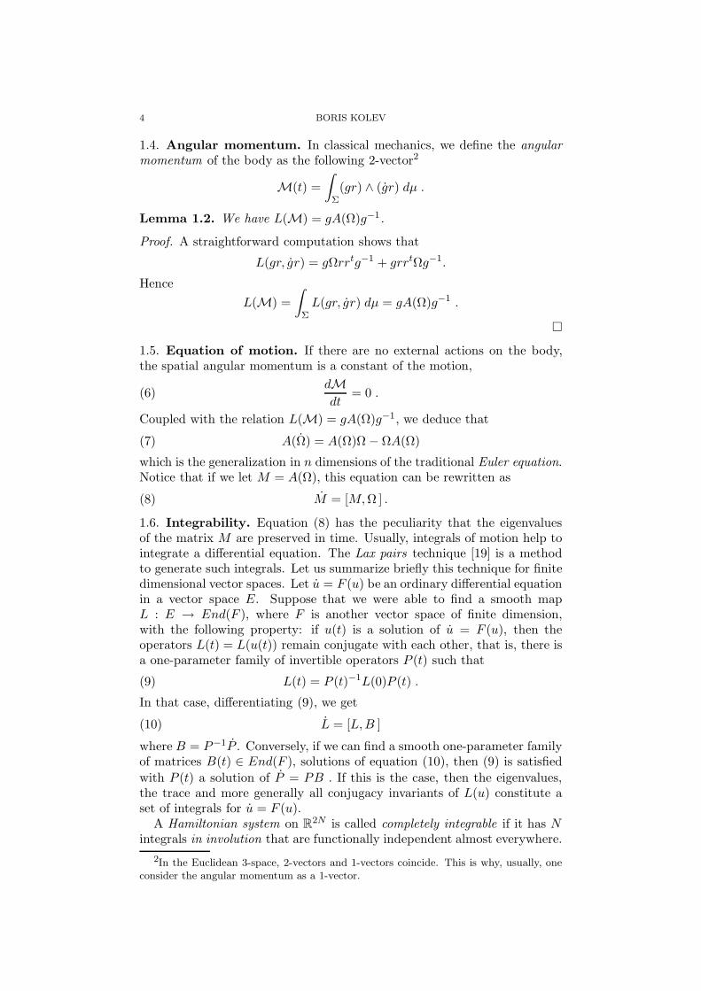
1.4. Angular momentum. In classical mechanics, we define the angularmomentum of the body as the following 2-vector2

M(t) =

∫

Σ(gr) ∧ (gr) dµ .

Lemma 1.2. We have L(M) = gA(Ω)g−1.

Proof. A straightforward computation shows that

L(gr, gr) = gΩrrtg−1 + grrtΩg−1.

Hence

L(M) =

∫

ΣL(gr, gr) dµ = gA(Ω)g−1 .

1.5. Equation of motion. If there are no external actions on the body,the spatial angular momentum is a constant of the motion,

(6)dM

dt= 0 .

Coupled with the relation L(M) = gA(Ω)g−1, we deduce that

(7) A(Ω) = A(Ω)Ω − ΩA(Ω)

which is the generalization in n dimensions of the traditional Euler equation.Notice that if we let M = A(Ω), this equation can be rewritten as

(8) M = [M,Ω ] .

1.6. Integrability. Equation (8) has the peculiarity that the eigenvaluesof the matrix M are preserved in time. Usually, integrals of motion help tointegrate a differential equation. The Lax pairs technique [19] is a methodto generate such integrals. Let us summarize briefly this technique for finitedimensional vector spaces. Let u = F (u) be an ordinary differential equationin a vector space E. Suppose that we were able to find a smooth mapL : E → End(F ), where F is another vector space of finite dimension,with the following property: if u(t) is a solution of u = F (u), then theoperators L(t) = L(u(t)) remain conjugate with each other, that is, there isa one-parameter family of invertible operators P (t) such that

(9) L(t) = P (t)−1L(0)P (t) .

In that case, differentiating (9), we get

(10) L = [L,B ]

where B = P−1P . Conversely, if we can find a smooth one-parameter familyof matrices B(t) ∈ End(F ), solutions of equation (10), then (9) is satisfied

with P (t) a solution of P = PB . If this is the case, then the eigenvalues,the trace and more generally all conjugacy invariants of L(u) constitute aset of integrals for u = F (u).

A Hamiltonian system on R2N is called completely integrable if it has N

integrals in involution that are functionally independent almost everywhere.

2In the Euclidean 3-space, 2-vectors and 1-vectors coincide. This is why, usually, oneconsider the angular momentum as a 1-vector.

LIE GROUPS AND MECHANICS 5

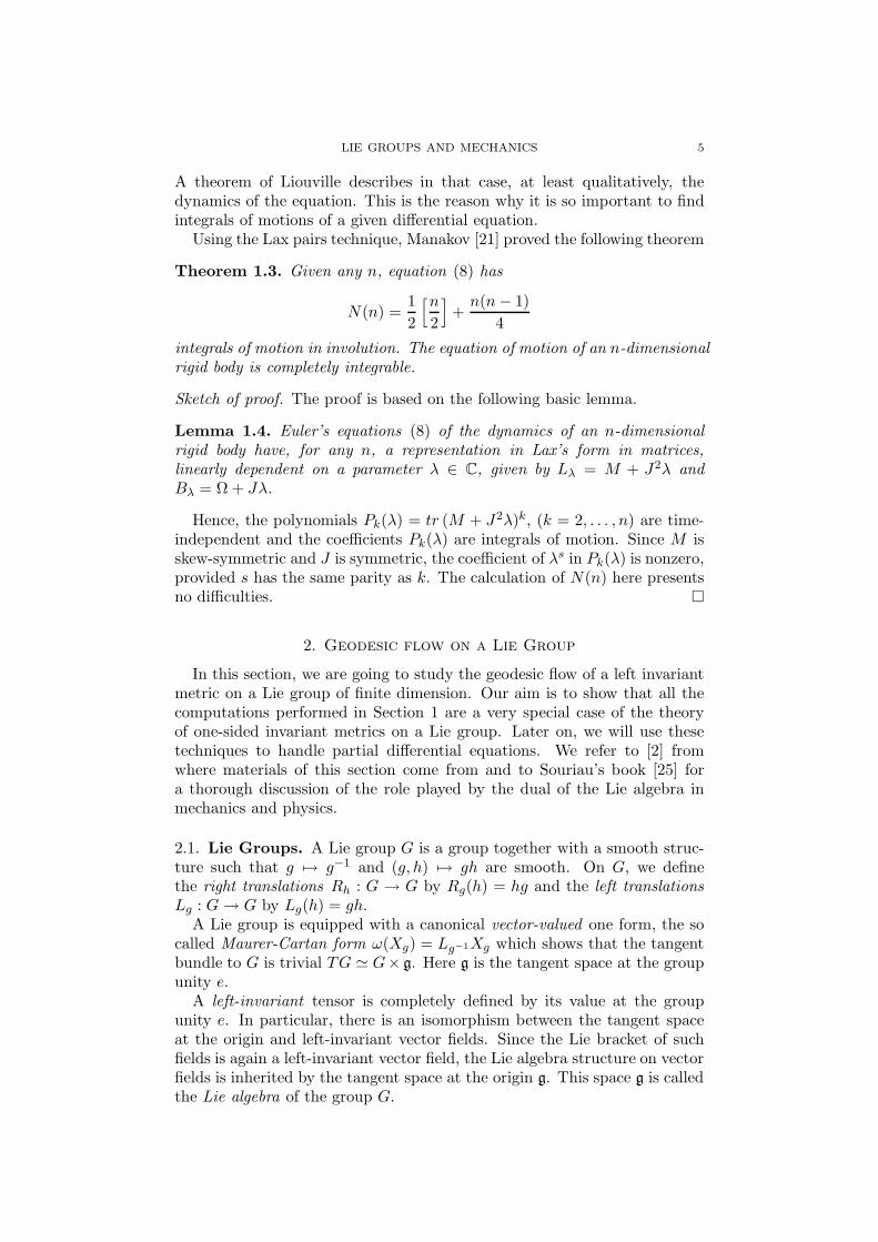
A theorem of Liouville describes in that case, at least qualitatively, thedynamics of the equation. This is the reason why it is so important to findintegrals of motions of a given differential equation.

Using the Lax pairs technique, Manakov [21] proved the following theorem

Theorem 1.3. Given any n, equation (8) has

N(n) =1

2

[n

2

]

+n(n− 1)

4

integrals of motion in involution. The equation of motion of an n-dimensionalrigid body is completely integrable.

Sketch of proof. The proof is based on the following basic lemma.

Lemma 1.4. Euler’s equations (8) of the dynamics of an n-dimensionalrigid body have, for any n, a representation in Lax’s form in matrices,linearly dependent on a parameter λ ∈ C, given by Lλ = M + J2λ andBλ = Ω + Jλ.

Hence, the polynomials Pk(λ) = tr (M + J2λ)k, (k = 2, . . . , n) are time-independent and the coefficients Pk(λ) are integrals of motion. Since M isskew-symmetric and J is symmetric, the coefficient of λs in Pk(λ) is nonzero,provided s has the same parity as k. The calculation of N(n) here presentsno difficulties.

2. Geodesic flow on a Lie Group

In this section, we are going to study the geodesic flow of a left invariantmetric on a Lie group of finite dimension. Our aim is to show that all thecomputations performed in Section 1 are a very special case of the theoryof one-sided invariant metrics on a Lie group. Later on, we will use thesetechniques to handle partial differential equations. We refer to [2] fromwhere materials of this section come from and to Souriau’s book [25] fora thorough discussion of the role played by the dual of the Lie algebra inmechanics and physics.

2.1. Lie Groups. A Lie group G is a group together with a smooth struc-ture such that g 7→ g−1 and (g, h) 7→ gh are smooth. On G, we definethe right translations Rh : G → G by Rg(h) = hg and the left translationsLg : G→ G by Lg(h) = gh.

A Lie group is equipped with a canonical vector-valued one form, the socalled Maurer-Cartan form ω(Xg) = Lg−1Xg which shows that the tangentbundle to G is trivial TG ≃ G× g. Here g is the tangent space at the groupunity e.

A left-invariant tensor is completely defined by its value at the groupunity e. In particular, there is an isomorphism between the tangent spaceat the origin and left-invariant vector fields. Since the Lie bracket of suchfields is again a left-invariant vector field, the Lie algebra structure on vectorfields is inherited by the tangent space at the origin g. This space g is calledthe Lie algebra of the group G.

6 BORIS KOLEV

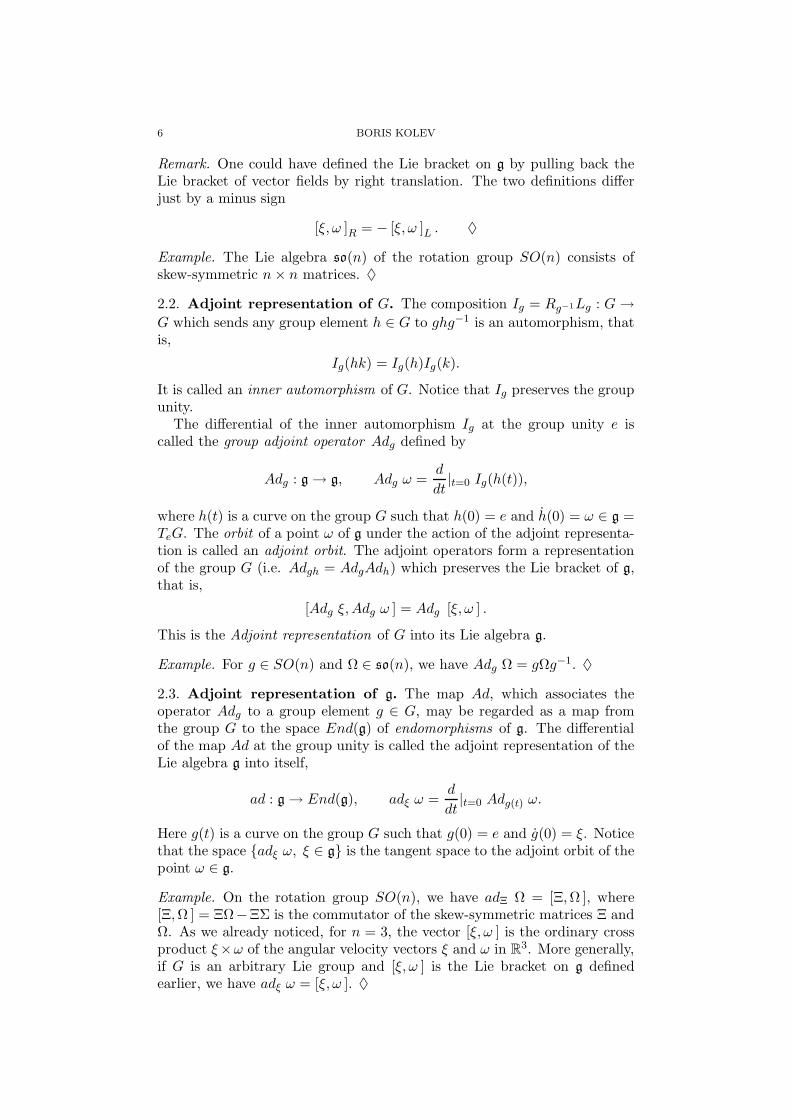
Remark. One could have defined the Lie bracket on g by pulling back theLie bracket of vector fields by right translation. The two definitions differjust by a minus sign

[ξ, ω ]R = − [ξ, ω ]L . ♦

Example. The Lie algebra so(n) of the rotation group SO(n) consists ofskew-symmetric n× n matrices. ♦

2.2. Adjoint representation of G. The composition Ig = Rg−1Lg : G →

G which sends any group element h ∈ G to ghg−1 is an automorphism, thatis,

Ig(hk) = Ig(h)Ig(k).

It is called an inner automorphism of G. Notice that Ig preserves the groupunity.

The differential of the inner automorphism Ig at the group unity e iscalled the group adjoint operator Adg defined by

Adg : g → g, Adg ω =d

dt|t=0 Ig(h(t)),

where h(t) is a curve on the group G such that h(0) = e and h(0) = ω ∈ g =TeG. The orbit of a point ω of g under the action of the adjoint representa-tion is called an adjoint orbit. The adjoint operators form a representationof the group G (i.e. Adgh = AdgAdh) which preserves the Lie bracket of g,that is,

[Adg ξ,Adg ω ] = Adg [ξ, ω ] .

This is the Adjoint representation of G into its Lie algebra g.

Example. For g ∈ SO(n) and Ω ∈ so(n), we have Adg Ω = gΩg−1. ♦

2.3. Adjoint representation of g. The map Ad, which associates theoperator Adg to a group element g ∈ G, may be regarded as a map fromthe group G to the space End(g) of endomorphisms of g. The differentialof the map Ad at the group unity is called the adjoint representation of theLie algebra g into itself,

ad : g → End(g), adξ ω =d

dt|t=0 Adg(t) ω.

Here g(t) is a curve on the group G such that g(0) = e and g(0) = ξ. Noticethat the space adξ ω, ξ ∈ g is the tangent space to the adjoint orbit of thepoint ω ∈ g.

Example. On the rotation group SO(n), we have adΞ Ω = [Ξ,Ω ], where[Ξ,Ω ] = ΞΩ−ΞΣ is the commutator of the skew-symmetric matrices Ξ andΩ. As we already noticed, for n = 3, the vector [ξ, ω ] is the ordinary crossproduct ξ×ω of the angular velocity vectors ξ and ω in R

3. More generally,if G is an arbitrary Lie group and [ξ, ω ] is the Lie bracket on g definedearlier, we have adξ ω = [ξ, ω ]. ♦

LIE GROUPS AND MECHANICS 7

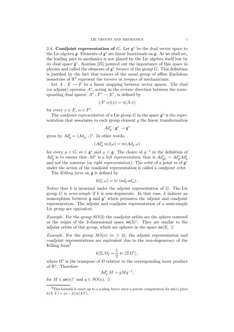
2.4. Coadjoint representation of G. Let g∗ be the dual vector space tothe Lie algebra g. Elements of g∗ are linear functionals on g. As we shall see,the leading part in mechanics is not played by the Lie algebra itself but byits dual space g∗. Souriau [25] pointed out the importance of this space inphysics and called the elements of g∗ torsors of the group G. This definitionis justified by the fact that torsors of the usual group of affine Euclideanisometries of R

3 represent the torsors or torques of mechanicians.Let A : E → F be a linear mapping between vector spaces. The dual

(or adjoint) operator A∗, acting in the reverse direction between the corre-sponding dual spaces, A∗ : F ∗ → E∗, is defined by

(A∗ α)(x) = α(A x)

for every x ∈ E, α ∈ F ∗.The coadjoint representation of a Lie group G in the space g∗ is the repre-

sentation that associates to each group element g the linear transformation

Ad∗g : g∗ → g

∗

given by Ad∗g = (Adg−1)∗. In other words,

(Ad∗g m)(ω) = m(Adg ω)

for every g ∈ G, m ∈ g∗ and ω ∈ g. The choice of g−1 in the definition ofAd∗g is to ensure that Ad∗ is a left representation, that is Ad∗gh = Ad∗gAd

∗h

and not the converse (or right representation). The orbit of a point m of g∗

under the action of the coadjoint representation is called a coadjoint orbit.The Killing form on g is defined by

k(ξ, ω) = tr (adξ adω) .

Notice that k is invariant under the adjoint representation of G. The Liegroup G is semi-simple if k is non-degenerate. In that case, k induces anisomorphism between g and g∗ which permutes the adjoint and coadjointrepresentation. The adjoint and coadjoint representation of a semi-simpleLie group are equivalent.

Example. For the group SO(3) the coadjoint orbits are the sphere centeredat the origin of the 3-dimensional space so(3)∗. They are similar to theadjoint orbits of this group, which are spheres in the space so(3). ♦

Example. For the group SO(n) (n ≥ 3), the adjoint representation andcoadjoint representations are equivalent due to the non-degeneracy of theKilling form3

k(Ξ,Ω) =1

2tr (Ξ Ω∗) ,

where Ω∗ is the transpose of Ω relative to the corresponding inner productof R

n. Therefore

Ad∗g M = gMg−1,

for M ∈ so(n)∗ and g ∈ SO(n). ♦

3This formula is exact up to a scaling factor since a precise computation for so(n) givesk(X, Y ) = (n − 2) tr(XY ).

8 BORIS KOLEV

Despite the previous two examples, in general the coadjoint and the ad-joint representations are not alike. For example, this is the case for thePoincare group (the non-homogenous Lorentz group) cf. [13].

2.5. Coadjoint representation of g. Similar to the adjoint representationof g, there is the coadjoint representation of g. This later is defined as thedual of the adjoint representation of g, that is,

ad∗ : g → End(g∗), ad∗ξ m = (adξ)∗(m) = −

d

dt|t=0 Ad

∗g(t) m,

where g(t) is a curve on the group G such that g(0) = e and g(0) = ξ.

Example. For Ω ∈ so(n) and M ∈ so(n)∗, we have ad∗ΩM = − [Ω,M ]. ♦

Given m ∈ g∗, the vectors ad∗ξ m, with various ξ ∈ g, constitute thetangent space to the coadjoint orbit of the point m.

2.6. Left invariant metric on G. A Riemannian or pseudo-Riemannianmetric on a Lie group G is left invariant if it is preserved under every leftshift Lg, that is,

〈Xg, Yg 〉g = 〈LhXg, Lh Yg 〉hg , g, h ∈ G.

A left-invariant metric is uniquely defined by its restriction to the tangentspace to the group at the unity, hence by a quadratic form on g. To such aquadratic form on g, a symmetric operator A : g → g∗ defined by

〈ξ, ω 〉 = (Aξ, ω ) = (Aω, ξ ) , ξ, ω ∈ g ,

is naturally associated, and conversely4. The operator A is called the inertiaoperator. A can be extended to a left-invariant tensor Ag : TgG → TgG

∗

defined by Ag = L∗g−1ALg−1 . More precisely, we have

〈X,Y 〉g = (AgX,Y )g

= (AgY,X )g, X, Y ∈ TgG.

The Levi-Civita connection of a left-invariant metric is itself left-invariant:if La and Lb are left-invariant vector fields, so is ∇La

Lb. We can write downan expression for this connection using the operator B : g × g → g definedby

(11) 〈[a, b ] , c 〉 = 〈B(c, a), b 〉

for every a, b, c in g. An exact expression for B is

B(a, b) = A−1 ad∗b(Aa) .

With these definitions, we get

(12) (∇LaLb)(e) =

1

2[a, b ] −

1

2B(a, b) +B(b, a)

4The round brackets correspond to the natural pairing between elements of g and g∗.

LIE GROUPS AND MECHANICS 9

2.7. Geodesics. Geodesics are defined as extremals of the Lagrangian

(13) L(g) =

∫

K (g(t), g(t)) dt

where

(14) K(X) =1

2〈Xg,Xg 〉g =

1

2(AgXg,Xg )g

is called the kinetic energy or energy functional.If g(t) is a geodesic, the velocity g(t) can be translated to the identity via

left or right shifts and we obtain two elements of the Lie algebra g,

ωL = Lg−1 g, ωR = Rg−1 g,

called the left angular velocity, respectively the right angular velocity. Let-ting m = Ag g ∈ TgG

∗, we define the left angular momentum mL and theright angular momentum mR by

mL = L∗gm ∈ g

∗, mR = R∗gm ∈ g

∗.

Between these four elements, we have the relations

(15) ωR = Adg ωL, mR = Ad∗gmL, mL = AωL.

Note that the kinetic energy is given by the formula

(16) K =1

2〈g, g 〉g =

1

2〈ωL, ωL 〉 =

1

2(mL, ωL ) =

1

2(Ag g, g )

g.

Example. The kinetic energy of an n-dimensional rigid body, defined by

(17) K(t) =1

2

∫

Σ‖g r‖2 dµ = −

1

2tr(ΩJΩ)

is clearly a left-invariant Riemannian metric on SO(n). In this example, wehave Ω = ωL and M = mL. Physically, the left-invariance is justified bythe fact that the physics of the problem must not depend on a particularchoice of reference frame used to describe it. It is a special case of Galileaninvariance. ♦

2.8. Euler-Arnold equation. The invariance of the energy with respectto left translations leads to the existence of a momentum map µ : TG→ g∗

defined by

µ((g, g))(ξ) =∂K

∂gZξ = 〈g, Rg ξ 〉g = (m,Rg ξ ) =

(

R∗gm, ξ

)

= mR(ξ),

where Zξ is the right-invariant vector field generated by ξ ∈ g. Accordingto Noether’s theorem [25], this map is constant along a geodesic, that is

(18)dmR

dt= 0.

As we did in the special case of the group SO(n), using the relation mR =Ad∗gmL and computing the time derivative, we obtain

(19)dmL

dt= ad∗ωL

mL.

10 BORIS KOLEV

This equation is known as the Arnold-Euler equation. Using ωL = A−1mL,it can be rewritten as an evolution equation on the Lie algebra

(20)dωLdt

= B(ωL, ωL) .

Remark. The Euler-Lagrange equations of problem (17) are given by

(21)

g = Lg ωL ,ωL = B(ωL, ωL) .

If the metric is bi-invariant, then B(a, b) = 0 for all a, b ∈ g and ωL isconstant. In that special case, geodesics are one-parameter subgroups, asexpected. ♦

2.9. Lie-Poisson structure on g∗. A Poisson structure on a manifold Mis a skew-symmetric bilinear function , that associates to a pair of smoothfunctions on the manifold a third function, and which satisfies the Jacobiidentity

f, g , h + g, h , f + h, f , g = 0

as well as the Leibniz identity

f, gh = f, g h+ g f, h .

On the torsor space g∗ of a Lie group G, there is a natural Poisson struc-ture defined by

(22) f, g (m) = (m, [dmf, dmg ])

for m ∈ g∗ and f, g ∈ C∞(g∗). Note that the differential of f at each pointm ∈ g∗ is an element of the Lie algebra g itself. Hence, the commutator[dm f, dm g ] is also a vector of this Lie algebra. The operation defined aboveis called the natural Lie-Poisson structure on the dual space to a Lie algebra.For more materials on Poisson structures, we refer to [20, 26].

Remark. A Poisson structure on a vector space E is linear if the Poissonbracket of two linear functions is itself a linear function. This property issatisfied by the Lie-Poisson bracket on the torsors space g∗ of a Lie groupG. ♦

To each function H on a Poisson manifold M one can associate a vectorfield ξH defined by

LξH f = H, f

and called the Hamiltonian field of H. Notice that

[ξF , ξH ] = ξF,H .

Conversely, a vector field v on a Poisson manifold is said to be Hamiltonianif there exists a function H such that v = ξH .

Example. On the torsors space g∗ of a Lie group G, the Hamiltonian fieldof a function H for the natural Lie-Poisson structure is given by ξH(m) =ad∗dmH

m.Let A be the inertia operator associated to a left-invariant metric on G.

Then equation (19) on g∗ is Hamiltonian with quadratic Hamiltonian

H(m) =1

2

(

A−1m,M)

, m ∈ g∗,

LIE GROUPS AND MECHANICS 11

which is nothing else but the kinetic energy expressed in terms of m = Aω.Notice that since mL(t) = Ad∗

g(t) mR where mR ∈ g∗ is a constant, each

integral curve mL(t) of this equation stays on a coadjoint orbit. ♦

A Poisson structure on a manifold M is non-degenerate if it derives froma symplectic structure on M . That is

f, g = ω(ξf , ξg) ,

where ω is a non-degenerate closed two form on M . Unfortunately, the Lie-Poisson structure on g∗ is degenerate in general. However, the restrictionof this structure on each coadjoint orbit is non-degenerate. The symplecticstructure on each coadjoint orbit is known as the Kirillov5 form. It is givenby

ω(ad∗am,ad∗b m) = (m, [a, b ] )

where a, b ∈ g and m ∈ g∗. Recall that the tangent space to the coadjointorbit of m ∈ g∗ is spanned by the vectors ad∗ξm where ξ describes g.

3. Right-invariant metric on the diffeomorphism group

In [1], Arnold showed that Euler equations of an incompressible fluid maybe viewed as the geodesic flow of a right-invariant metric on the group ofvolume-preserving diffeomorphism of a 3-dimensional Riemannian manifoldM (filled by the fluid). More precisely, let G = Diffµ(M) be the groupof diffeomorphisms preserving a volume form µ on some closed Riemannianmanifold M . According to the Action Principle, motions of an ideal (incom-pressible and inviscid) fluid in M are geodesics of a right-invariant metricon Diffµ(M). Such a metric is defined by a quadratic form K (the kineticenergy) on the Lie algebra Xµ(M) of divergence-free vector fields

K =1

2

∫

M

‖v‖2 dµ

where ‖v‖2 is the square of the Riemannian length of a vector field v ∈X (M). An operator B on Xµ(M) ×Xµ(M) defined by the relation

〈[u, v ] , w 〉 = 〈B(w, u), v 〉

exists. It is given by the formula

B(u, v) = curlu× v + grad p ,

where × is the cross product and p a function on M defined uniquely (mod-ulo an additive constant) by the condition divB = 0 and the tangency ofB(u, v) to ∂M . The Euler equation for ideal hydrodynamics is the evolutionequation

(23)∂u

∂t= u× curlu− grad p .

If at least formally, the theory works as well in infinite dimension and theunifying concepts it brings form a beautiful piece of mathematics, the detailsof the theory are far from being as clear as in finite dimension. The mainreason of these difficulties is the fact that the diffeomorphism group is just a

5Jean-Marie Souriau has generalized this construction for other natural G-actions ong∗ when the group G has non null symplectic cohomology [25].

12 BORIS KOLEV

Frechet Lie group, where the main theorems of differential geometry like theCauchy-Lipschitz theorem and the Inverse function theorem are no longervalid.

In this section, we are going to apply the results of Section 2 to study thegeodesic flow of a Hk right-invariant metrics on the diffeomorphism groupof the circle S

1. This may appear to be less ambitious than to study the 3-dimensional diffeomorphism group. However, we will be able to understandin that example some phenomena which may lead to understand why the3-dimensional ideal hydrodynamics is so difficult to handle. Moreover, weshall give an example where things happen to work well, the Camassa-Holmequation.

3.1. The diffeomorphism group of the circle. The group Diff(S1) isan open subset of C∞(S1,S1) which is itself a closed subset of C∞(S1,C).We define a local chart (U0,Ψ0) around a point ϕ0 ∈ Diff(S1) by theneighborhood

U0 =

‖ϕ− ϕ0‖C0(S1) < 1/2

of ϕ0 and the map

Ψ0(ϕ) =1

2πilog(ϕ0(x)ϕ(x)) = u(x), x ∈ S

1.

The structure described above endows Diff(S1) with a smooth manifoldstructure based on the Frechet space C∞(S1). The composition and the in-verse are both smooth maps Diff(S1)×Diff(S1) → Diff(S1), respectivelyDiff(S1) → Diff(S1), so that Diff(S1) is a Lie group.

A tangent vector V at a point ϕ ∈ Diff(S1) is a function V : S1 → TS

1

such that π(V (x)) = ϕ(x). It is represented by a pair (ϕ, v) ∈ Diff(S1) ×C∞(S1). Left and right translations are smooth maps and their derivativesat a point ϕ ∈ Diff(S1) are given by

Lψ V = (ψ(ϕ), ψx(ϕ) v)

Rψ V = (ϕ(ψ), v(ψ))

The adjoint action on g = V ect(S1) ≡ C∞(S1) is

Adψ u = ψx(ψ−1)u(ψ−1),

whereas the Lie bracket on the Lie algebra TIdDiff(S1) = V ect(S1) ≡C∞(S1) of Diff(S1) is given by

[u, v] = −(uxv − uvx), u, v ∈ C∞(S1)

Each v ∈ V ect(S1) gives rise to a one-parameter subgroup of diffeomor-phisms η(t, ·) obtained by solving

(24) ηt = v(η) in C∞(S1)

with initial data η(0) = Id ∈ Diff(S1). Conversely, each one-parametersubgroup t 7→ η(t) ∈ Diff(S1) is determined by its infinitesimal generator

v =∂

∂tη(t)

∣

∣

∣

t=0∈ V ect(S1).

Evaluating the flow t 7→ η(t, ·) of (24) at t = 1 we obtain an element expL(v)of Diff(S1). The Lie-group exponential map v → expL(v) is a smooth map

LIE GROUPS AND MECHANICS 13

of the Lie algebra to the Lie group [23]. Although the derivative of expL at0 ∈ C∞(S1) is the identity, expL is not locally surjective [23]. This failure, incontrast with the case of Hilbert Lie groups [18], is due to the fact that theinverse function theorem does not necessarily hold in Frechet spaces [15].

3.2. Hk metrics on Diff(S1). For k ≥ 0 and u, v ∈ V ect(S1) ≡ C∞(S1),we define

(25) 〈u, v〉k =

∫

S1

k∑

i=0

(∂ixu) (∂ixv) dx =

∫

S1

Ak(u) v dx ,

where

(26) Ak = 1 −d2

dx2+ ...+ (−1)k

d2k

dx2k

is a continuous linear isomorphism of C∞(S1). Note that Ak is a symmetricoperator for the L2 inner product

∫

S1

Ak(u) v dx =

∫

S1

uAk(v) dx.

Remark. What should be g∗ for G = Diff(S1) and g = vect(S1) ? If we letg∗ be the space of distributions, Ak is no longer an isomorphism. This is thereason why we restrict g∗ to the range of Ak

Im(Ak) = C∞(S1).

The pairing between g and g∗ is then given by the L2 inner product

(m,u ) =

∫

S1

mudx.

With these definitions, the coadjoint action of Diff(S1) on g∗ = C∞(S1) isgiven by

Ad∗ϕm =1

(ϕx(ϕ−1))2m(ϕ−1).

Notice that this formula corresponds exactly to the action of the diffeomor-phism group Diff(S1) on quadratic differentials of the circle (expressionsof the form m(x) dx2). This is the reason why one generally speaks of thetorsor space of the group Diff(S1) as the space of quadratic differentials.♦

We obtain a smooth right-invariant metric on Diff(S1) by extending theinner product (25) to each tangent space TϕDiff(S1), ϕ ∈ Diff(S1), byright-translations i.e.

〈V,W 〉ϕ =⟨

Rϕ−1V,Rϕ−1W⟩

k, V,W ∈ TϕDiff(S1).

The existence of a connection compatible with the metric is ensured (see[10]) by the existence of a bilinear operator B : C∞(S1)×C∞(S1) → C∞(S1)such that

〈B(u, v), w〉 = 〈u, [v,w]〉, u, v, w ∈ V ect(S1) = C∞(S1).

For the Hk metric, this operator is given by (see [11])

(27) Bk(u, v) = −A−1k

(

2vxAk(u) + vAk(ux))

, u, v ∈ C∞(S1).

14 BORIS KOLEV

3.3. Geodesics. The existence of the connection ∇k enables us to definethe geodesic flow. A C2-curve ϕ : I → Diff(S1) such that ∇ϕ ϕ = 0, whereϕ denotes the time derivative ϕt of ϕ, is called a geodesic. As we did inSection 2, in the case of a left-invariant metric, we let

u(t) = Rϕ−1 ϕ = ϕt ϕ−1

which is the right angular velocity on the group Diff(S1). Therefore, acurve ϕ ∈ C2(I,Diff(S1)) with ϕ(0) = Id is a geodesic if and only if

(28) ut = Bk(u, u), t ∈ I.

Equation (28) is the Euler-Arnold equation associated to the right-invariantmetric (25). Here are two examples of problems of type (28) on Diff(S1)which arise in mechanics.

Example. For k = 0, that is for the L2 right-invariant metric, equation (28)becomes the inviscid Burgers equation

(29) ut + 3uux = 0.

All solutions of (29) but the constant functions have a finite life span and(29) is a simplified model for the occurrence of shock waves in gas dynamics(see [16]). ♦

Example. For k = 1, that is for the H1 right-invariant metric, equation (28)becomes the Camassa-Holm equation (cf. [24])

(30) ut + uux + ∂x (1 − ∂x2)−1

(

u2 +1

2ux2

)

= 0.

Equation (30) is a model for the unidirectional propagation of shallow wa-ter waves [3, 17]. It has a bi-Hamiltonian structure [14] and is completelyintegrable [12]. Some solutions of (30) exist globally in time [5, 6], whereasothers develop singularities in finite time [6, 7, 8, 22]. The blowup phe-nomenon can be interpreted as a simplified model for wave breaking – thesolution (representing the water’s surface) stays bounded while its slopebecomes unbounded [8]. ♦

3.4. The momentum. As a consequence of the right-invariance of the met-ric by the action of the group on itself, we obtain the conservation of theleft angular momentum mL along a geodesic ϕ. Since mL = Ad∗

ϕ−1 mR and

mR = Ak(u), we get that

(31) mk(ϕ, t) = Ak(u) ϕ · ϕ2x,

satisfies mk(t) = mk(0) as long as mk(t) is defined.

3.5. Existence of the geodesics. In a local chart the geodesic equation(28) can be expressed as the Cauchy problem

(32)

ϕt = v,vt = Pk(ϕ, v),

with ϕ(0) = Id, v(0) = u(0). However, the local existence theorem fordifferential equations with smooth right-hand side, valid for Hilbert spaces[18], does not hold in C∞(S1) (see [15]) and we cannot conclude at thisstage. However, in [11], we proved

LIE GROUPS AND MECHANICS 15

Theorem 3.1. Let k ≥ 1. For every u0 ∈ C∞(S1), there exists a uniquegeodesic ϕ ∈ C∞([0, T ),Diff(S1)) for the metric (25), starting at ϕ(0) =Id ∈ Diff(S1) in the direction u0 = ϕt(0) ∈ V ect(S1). Moreover, thesolution depends smoothly on the initial data u0 ∈ C∞(S1).

Sketch of proof. The operator Pk in (32) is specified by

Pk(ϕ, v) =[

Qk(v ϕ−1)

]

ϕ,

where Qk : C∞(S1) → C∞(S1) is defined by Qk(w) = Bk(w,w) + wwx.Since

C∞(S1) =⋂

r≥n

Hr(S1)

for all n ≥ 0, we may consider the problem (32) on each Hilbert spaceHn(S1). If k ≥ 1 and n ≥ 3, then Pk is a smooth map from Un ×Hn(S1)to Hn(S1), where Un ⊂ Hn(S1) is the open subset of all functions havinga strictly positive derivative. The classical Cauchy-Lipschitz theorem inHilbert spaces [18] yields the existence of a unique solution ϕn(t) ∈ Un of(32) for all t ∈ [0, Tn) for some maximal Tn > 0. Relation (31) can then beused to prove that Tn = Tn+1 for all n ≥ 3.

Remark. For k = 0, in problem (32), we obtain

P0(ϕ, v) = −2v · vxϕx

which is not an operator from Un × Hn(S1) into Hn(S1) and the proofof Theorem 3.1 is no longer valid. However, in that case, the method ofcharacteristics can be used to show that even for k = 0 the geodesics existsand are smooth (see [10]). ♦

3.6. The exponential map. The previous results enable us to define theRiemannian exponential map exp for the Hk right-invariant metric (k ≥ 0).In fact, there exists δ > 0 and T > 0 so that for all u0 ∈ Diff(S1) with‖u0‖2k+1 < δ the geodesic ϕ(t;u0) is defined on [0, T ] and we can defineexp(u0) = ϕ(1;u0) on the open set

U =

u0 ∈ Diff(S1) : ‖u0‖2k+1 <2 δ

T

of Diff(S1). The map u0 7→ exp(u0) is smooth and its Frechet derivativeat zero, Dexp0, is the identity operator. On a Frechet manifold, these factsalone do not necessarily ensure that exp is a smooth local diffeomorphism[15]. However, in [11], we proved

Theorem 3.2. The Riemannian exponential map for the Hk right-invariantmetric on Diff(S1), k ≥ 1, is a smooth local diffeomorphism from a neigh-borhood of zero on V ect(S1) to a neighborhood of Id on Diff(S1).

Sketch of proof. Working in Hk+3(S1), we deduce from the inverse functiontheorem in Hilbert spaces that exp is a smooth diffeomorphism from anopen neighborhood Ok+3 of 0 ∈ Hk+3(S1) to an open neighborhood Θk+3

of Id ∈ Uk+3.We may choose Ok+3 such that Dexpu0

is a bijection of Hk+3(S1) forevery u0 ∈ Ok+3. Given n ≥ k + 3, using (31) and the geodesic equation,

16 BORIS KOLEV

we conclude that there is no u0 ∈ Hn(S1) \Hn+1(S1), with exp(u0) ∈ Un+1.We have proved that for every n ≥ k + 3,

exp : O = Ok+3 ∩ C∞(S1) → Θ = Θk+3 ∩ C∞(S1)

is a bijection. Using similar arguments, (31) and the geodesic equation canbe used to prove that there is no u0 ∈ Hn(S1)\Hn+1(S1), with Dexpu0

(v) ∈

Hn+1(S1) for some u0 ∈ O. Hence, for every u0 ∈ O and n ≥ k + 3, thebounded linear operator Dexpu0

is a bijection from Hn(S1) to Hn(S1).

Remark. For k = 0 we have that exp is not a C1 local diffeomorphism froma neighborhood of 0 ∈ V ect(S1) to a neighborhood of Id ∈ Diff(S1), asproved in [10]. The crucial difference with the case (k ≥ 1) lies in the factthat the inverse of the operator Ak, defined by (26), is not regularizing.This feature makes the previous approach inapplicable but the existence ofgeodesics can nevertheless be proved by the method of characteristics. ♦

References

[1] Arnold VI, Sur la geometrie differentielle des groupes de Lie de dimensioninfinie et ses applications a l’hydrodynamique des fluides parfaits, Ann. Inst.Fourier (Grenoble) 16 (1966), 319–361.

[2] Arnold VI and Khesin BA, Topological Methods in Hydrodynamics, Springer-Verlag, New York, 1998.

[3] Camassa R and Holm DD, An integrable shallow water equation with peakedsolitons, Phys. Rev. Lett. 71 (1993), 1661–1664.

[4] Camassa R, Holm DD and Hyman J, A new integrable shallow water equation,Adv. Appl. Mech. 31 (1994), 1–33.

[5] Constantin A, On the Cauchy problem for the periodic Camassa-Holm equa-tion, J. Differential Equations 141 (1997), 218–235.

[6] Constantin A and Escher J, Well-posedness global existence and blow-up phe-nomena for a periodic quasi-linear hyperbolic equation, Comm. Pure Appl.Math. 51 (1998), 475–504.

[7] Constantin A and Escher J, Wave breaking for nonlinear nonlocal shallow waterequations, Acta Math. 181 (1998), 229–243.

[8] Constantin A and Escher J, On the blow-up rate and the blow-up set of break-ing waves for a shallow water equation, Math. Z. 233 (2000), 75–91.

[9] Constantin A and Kolev B, Least action principle for an integrable shallowwater equation, J. Nonlinear Math. Phys. 8 (2001), 471–474.

[10] Constantin A and Kolev B, On the geometric approach to the motion of inertialmechanical systems, J. Phys. A 35 (2002), R51–R79.

[11] Constantin A and Kolev B, Geodesic flow on the diffeomorphism group of thecircle, Comment. Math. Helv. 78 (2003), 787–804.

[12] Constantin A and McKean HP, A shallow water equation on the circle, Comm.Pure Appl. Math. 52 (1999), 949–982.

[13] Cushman R and van der Kallen W, Adjoint and coadjoint orbits of the Poincaregroup, ArXiv math.RT/0305442 (2003).

[14] Fokas AS and Fuchssteiner B, Symplectic structures, their Backlund transfor-mations and hereditary symmetries, Phys. D 4 (1981), 47–66.

[15] Hamilton RS, The inverse function theorem of Nash and Moser, Bull. Amer.Math. Soc. (N.S.) 7 (1982), 65–222.

[16] Hormander L, Lectures on Nonlinear Hyperbolic Differential Equations,Springer-Verlag, Berlin, 1997.

LIE GROUPS AND MECHANICS 17

[17] Johnson RS, Camassa-Holm, Korteweg-de Vries and related models for waterwaves, J. Fluid Mech. 455 (2002), 63–82.

[18] Lang S, Fundamentals of Differential Geometry, Springer-Verlag, New York,1999.

[19] Lax PD, Integrals of nonlinear equations of evolution and solitary waves,Comm. Pure Appl. Math. 21 (1968), 467–490.

[20] Marsden JE and Ratiu TS, Introduction to mechanics and symmetry, Springer-Verlag, New York, 1999.

[21] Manakov SV, A remark on the integration of the Eulerian equations of thedynamics of an n-dimensional rigid body, Funkcional. Anal. i Prilozen. 10(1976), 93–94.

[22] McKean HP, Breakdown of a shallow water equation, Asian J. Math. 2 (1998),867–874.

[23] Milnor J, Remarks on infinite-dimensional Lie groups, in Relativity, Groupsand Topology, North-Holland, Amsterdam, 1984, 1009–1057.

[24] Misio lek G, A shallow water equation as a geodesic flow on the Bott-Virasorogroup, J. Geom. Phys. 24 (1998), 203–208.

[25] Souriau JM, Structure of Dynamical Systems, Birkhauser, Boston, 1997.[26] Weinstein A, The local structure of Poisson manifolds, J. Differential Geom.

18 (1983), 523–557.

CMI, 39, rue F. Joliot-Curie, 13453 Marseille cedex 13, France

E-mail address: boris.kolev@up.univ-mrs.fr