liens code de la propriété intellectuelle. articles l 122....
TRANSCRIPT

AVERTISSEMENT
Ce document est le fruit d'un long travail approuvé par le jury de soutenance et mis à disposition de l'ensemble de la communauté universitaire élargie. Il est soumis à la propriété intellectuelle de l'auteur. Ceci implique une obligation de citation et de référencement lors de l’utilisation de ce document. D'autre part, toute contrefaçon, plagiat, reproduction illicite encourt une poursuite pénale. Contact : [email protected]
LIENS Code de la Propriété Intellectuelle. articles L 122. 4 Code de la Propriété Intellectuelle. articles L 335.2- L 335.10 http://www.cfcopies.com/V2/leg/leg_droi.php http://www.culture.gouv.fr/culture/infos-pratiques/droits/protection.htm

Ecole doctorale IAEM Lorraine – Département de Formation Doctorale en Automatique
CRAN - Centre de Recherche en Automatique de Nancy
THÈSE
Présentée et soutenue publiquement le 10 Juillet 2017
pour l’obtention du
Doctorat de l’Université de Lorraine
(spécialité Automatique, Traitement du signal et des Images, Génie Informatique)
par
Anh HOANG
Pronostic de la performance d’Efficacité Energétique pour la prise de décision en
maintenance dans les systèmes industriels
Rapporteurs:
Christophe Berenguer - Professeur à l’Institut National Polytechnique de Grenoble, France
Mitra Fouladirad – Maître de conférences (HDR) à l’Université de Technologie de Troyes, France
Examinateurs:
Rossi Setchi - Professeur à l’Université de Cardiff, UK
Jay Lee - Professeur à l’Université de Cincinnati, USA
Olivier Senechal - Professeur à l’Université de Valenciennes et du Hainaut Cambrésis, France
Benoit Iung- Professeur à l’Université de Lorraine, France (Directeur de Thèse)
Phuc Do - Maître de conférences à l’Université de Lorraine, France (Co-directeur de Thèse)

Ecole doctorale IAEM Lorraine – Département de Formation Doctorale en Automatique
CRAN - Centre de Recherche en Automatique de Nancy
Mis en page avec la classe thloria.

Ecole doctorale IAEM Lorraine – Département de Formation Doctorale en Automatique
CRAN - Centre de Recherche en Automatique de Nancy
THESIS
Presented and publicly supported on July 10, 2017
to obtain the
Doctorate of Lorraine University (Specialty Automatic, Signal and Image Processing, Computer Engineering)
by
Anh HOANG
Energy Efficiency-Based Prognostics for Optimizing the Maintenance Decision-Making
in Industrial Systems
Reporters:
Christophe Berenguer - Professor of Grenoble Institute of Technology, France
Mitra Fouladirad – Associate professor of University of Technology of Troyes, France
Reviewers:
Rossi Setchi - Professor of Cardiff University, UK
Jay Lee - Professor of Cincinnati University, USA
Olivier Senechal - Professor of University of Valenciennes and Hainaut-Cambrésis, France
Benoit Iung- Professor of Lorraine University, France (Supervisor of Thesis)
Phuc Do - Associate professor of Lorraine University, France (Co-Supervisor of Thesis)

Ecole doctorale IAEM Lorraine – Département de Formation Doctorale en Automatique
CRAN - Centre de Recherche en Automatique de Nancy
This page intentionally left blank.

ii
Acknowledgements First of all, I would like to express my greatest appreciations and thanks to my supervisor
Professor Benoit IUNG, Lorraine University for his help, support, fruitful discussions, and
encouragement that made this thesis possible.
My special gratitude is given to my co-supervisor Dr. Phuc DO, who accepted me as his first
PhD student in Lorraine University, for his helpful and constructive comments, guidance and
continuous support.
I am also in acknowledgement of funding by the Ministry of Education and Training, Vietnam
(MOET) together with Vietnam International Education Development (VIED); without their
financial support, this thesis would not have been a possibility.
Finally, I would like to express my great gratefulness to my family and friends for their
consistent stimulation of my dream pursuit. I am deeply indebted to Trang Tran, my wife, for
her persistent and timely sacrifice and cheer when I needed them the most.
Nancy, July 2017

iii

iv
Abstract
Among sustainability consideration, energy is today the key for economic growth in industrial
systems. Energy resources are however limited and becomes more and more expensive. The
energy optimization of manufacturing systems must therefore be considered as a major
challenge to be compliant with environmental impact and management of energy resources.
This should be reflected primarily by using energy efficiency (EE) as main key lever to deploy
sustainability to plants, i.e. reduce the amount of energy required to provide products and
services.
With regards to this EE context, the aim of this thesis is to investigate the problem of
considering energy efficiency and its prediction as a new indicator in maintenance decision-
making. In that way, we develop first a concept of energy efficiency, called EEI (energy
efficiency indicator), applicable to the different levels of abstraction of an industrial system.
Then, we propose a generic formulation to evaluate the EEI (and its evolution) taking into
account static and dynamic factors of influence. The temporal evolution of this indicator with
respect to the degradation of the system is addressed in a predictive maintenance objective. It
leads to found an energy efficiency performance concept called REEL (remaining energy-
efficient lifetime), representing the residual energy lifetime. To predict the potential evolution
of the IEE to calculate REEL, a generic approach based on existing predictive approaches is
also developed. Next, we investigate the use of EE in CBM maintenance decision-making.
Finally, all these contributions are validated on the TELMA platform.

v

vi
Résumé Aujourd'hui, la maîtrise de l'énergie est la question prépondérante pour la croissance
économique des entreprises industrielles. En effet, l’énergie est une ressource qui se raréfie et
qui devient de plus en plus coûteuse. L’optimisation énergétique est donc un défi majeur que
doit relever les entreprises et principalement celles manufacturières pour supporter les
exigences du développement durable. Cette optimisation est à construire prioritairement par
une amélioration de l’efficacité énergétique (EE), c'est-à-dire réduire la quantité d'énergie
requise pour produire des produits et des services.
En regard de ce défi énergétique, l’objectif de cette thèse est d’investiguer la considération de
l’efficacité énergétique et de sa prévision comme un nouvel indicateur pertinent dans la prise
de décision en maintenance. En ce sens, nous proposons tout d'abord un concept de l’efficacité
énergétique, appelé EEI (EE indicator), applicable aux différents niveaux d’abstraction d’un
système industriel. Nous définissons ensuite une formulation générique permettant d’évaluer
l'EEI (et son évolution) en prenant en compte les facteurs d’influence statiques et dynamiques.
Cela nous amène à fonder un concept de performance d’efficacité énergétique, appelé REEL
(Remaining Energy-Efficient Lifetime), représentant la durée de vie énergétique résiduelle.
Pour prédire l’évolution potentielle de l’EEI qui permettra de calculer la REEL, une approche
générique basée sur des approches de pronostics existantes est également développée. Ensuite,
nous investiguons l'utilisation d’EE dans la prise de décision en maintenance conditionnelle
(Condition-Based Maintenance, CBM). Enfin, toutes ces contributions sont validées sur la
plateforme laboratoire TELMA.

vii

viii
Table of Contents General Introduction ............................................................................................................ 1
Chapter 1 An overview about energy efficiency in “green manufacturing” for
maintenance decision-making .............................................................................................. 7
1.1. Introduction ..................................................................................................................... 7
1.2. From sustainability in general… ...................................................................................... 7
1.3. To sustainability in manufacturing industry: Green manufacturing............................... 10
1.4. What is energy efficiency in general … and then in industry? ...................................... 15
1.4.1. Energy efficiency in general .............................................................................. 15
1.4.2. Energy efficiency in industry and mainly in manufacturing .............................. 16
1.5. How to integrate EEI/EEP in maintenance decision-making and more precisely in
CBM? .................................................................................................................................. 19
1.5.1. Classification of maintenance strategies ............................................................ 19
1.5.2. Is Energy Efficiency already integrated in maintenance and mainly CBM? ..... 23
1.6. Conclusions ................................................................................................................... 24
Chapter 2 Scientific problem statement on EE concept and its application in CBM
maintenance decision-making ............................................................................................ 27
2.1 Introduction .................................................................................................................... 27
2.2 How to define and evaluate/predict EEI/EEP at the different abstraction levels of an
industrial (manufacturing) system by considering the dynamics of this system? ................. 27
2.2.1 General concepts of EEI and their application in manufacturing systems ............ 27
2.2.2 EEI at each level of abstraction (component, function/system) of a
manufacturing
system ......................................................................................................................... 32
2.2.3 EEP concept for evaluating the residual life energy ............................................. 37
2.2.4 Evaluation of EEI/EEP in dynamic context .......................................................... 38
2.3 How to use EE in CBM strategies?................................................................................. 39
2.3.1 Using EE as main condition for CBM strategies .................................................. 39

ix
2.3.2 Evaluation of the EE-based CBM ......................................................................... 40
2.4 Conclusions .................................................................................................................... 41
Chapter 3 EEI and REEL: concept and formulation for industrial applications ......... 43
3.1. Introduction ............................................................................................................... 43
3.2. Concepts of energy efficiency indicators for industrial systems ............................... 43
3.2.1 Energy efficiency indicator at component level ................................................. 45
3.2.2 Energy efficiency indicator at the function/system level ................................... 47
3.3. Remaining Energy-Efficient Lifetime....................................................................... 49
3.3.1 Concept of the Remaining Energy-Efficient Lifetime .......................................... 49
3.3.2 Evaluation of the Remaining Energy-Efficient Lifetime at component level ....... 51
3.3.3 Evaluation of the Remaining Energy-Efficient Lifetime at higher level .............. 53
3.4. Conclusion ................................................................................................................ 55
Chapter 4 Generic approach for prognostics of the evolution of EEI and REEL ........ 57
4.1. Introduction ............................................................................................................... 57
4.2. Short review on existing prognostic approaches for RUL prediction ....................... 57
4.3. Global view of the proposed generic approach for prognostics of the EEI evolution
and REEL ............................................................................................................................. 59
4.4. Step 1: Energy efficiency modeling .......................................................................... 60
4.4.1. EEI at component level ...................................................................................... 61
4.4.2. EEI at higher level ............................................................................................. 64
4.5. Step 2: Prediction of the potential evolution of impact factors ................................. 65
4.5.1. At component level ............................................................................................ 65
4.5.2. At higher level ................................................................................................... 67
4.6. Step 3: Evaluation of the evolution of EEI and estimation of REEL ........................ 68
4.6.1. Phase 1: Evaluation of the evolution of EEI and estimation of REEL ............... 68
4.6.2. Phase 2: Online updating of the Remaining Energy-Efficient Lifetime ............ 69
4.7. Conclusion ................................................................................................................ 69
x
Chapter 5 Validation of the contributions in the case of TELMA platform ................. 71
5.1. Introduction ............................................................................................................... 71
5.2. Presentation of TELMA platform ............................................................................. 71
5.2.1 Identification and classification of key components and the function/system ... 73
5.2.2 Description of the system and experimentation ................................................. 73
5.3. Implementation of the generic approach for selection of EEI and related models:
architecture definition ........................................................................................................... 75
5.3.1 Step 1: Energy efficiency modeling ................................................................... 75
5.3.2 Step 2: Prediction of the evolution of impact factors ......................................... 82
5.3.3 Step 3: Evaluation of the potential evolution of EEI and estimation of REEL .. 84
5.4. Conclusion ................................................................................................................ 85
Chapter 6 Use of EE for CBM maintenance decision-making........................................ 87
6.1. Introduction ............................................................................................................... 87
6.2. General dicussions on EEI indicator for decision-making ........................................ 87
6.3. EEI-based CBM maintenance ................................................................................... 88
6.3.1. Maintenance decision rules ................................................................................ 89
6.3.2. Extension of a classical CBM policy ................................................................. 92
6.4. Implementation platform TELMA ........................................................................... 95
6.4.1. Maintenance optimization for MD1 ................................................................... 96
6.4.2. Sensitivity analyses ............................................................................................ 98
6.5. Conclusion .............................................................................................................. 101
General conclusion ........................................................................................................... 103
Publications of the Author ............................................................................................... 107
Bibliography ...................................................................................................................... 109
xi
Table of Figures Figure 1. The three pillars of sustainability ............................................................................ 8
Figure 2. Framework for Sustainable Manufacturing with the three pillars approach ......... 11
Figure 3. Future manufacturing system with the integration of IT system .......................... 12
Figure 4. Multiple benefits of energy efficiency .................................................................. 16
Figure 5. EE contributing to TBL of sustainable manufacturing frameworks ..................... 17
Figure 6: Simplified classification of maintenance strategies ............................................... 21
Figure 7. Structure of CBM decision-making ...................................................................... 23
Figure 8. Concepts of EEI and their potential applications .................................................. 44
Figure 9. Manufacturing system of 3 components ................................................................ 46
Figure 10. Illustration of the REEL and its variants ............................................................. 50
Figure 11. The REEL evalution at the component level ....................................................... 52
Figure 12. Procedure to evaluate REEL at function/system level ......................................... 54
Figure 13. Classification of prognostic approaches ............................................................. 58
Figure 14. Generic approach for prognostic of the evolution of EEI .................................... 59
Figure 15. Generic approach for prognostic of the EEI evolution to estimate the REEL ..... 60
Figure 16. Diagram for modeling energy efficiency of manufacturing systems ................... 62
Figure 17. Procedure for prognostics approach selection of energy consumption and useful
output modelling ................................................................................................................... 63
Figure 18. Energy flow and Air flow output of fan system .................................................. 64
Figure 19. Procedure for predicting the evolution of impact factors of the energy efficiency
model 66
Figure 20. Procedure for selecting prognostic approaches to predict the evolution of a
dynamic factor ...................................................................................................................... 67
Figure 21. Procedure to evaluate the evolution of EEIs and to estimate the REEL .............. 68
Figure 22. Structure of the platform TELMA ....................................................................... 72
Figure 23. Illustration of data sheet for recorded energy consumption ................................. 74
xii
Figure 24. Real energy consumption of MD1 in relationship with speed and deterioration
level 77
Figure 25. Calculated energy consumption of MD1 in relationship with speed and
deterioration level ................................................................................................................. 78
Figure 26. EEI of MD1 as a function of speed and bearing deterioration at the component
level 81
Figure 27. A forecasted mission profile (a) and the bearing deterioration evolution of two
motor-driven systems MD1 and MD2 (b) ............................................................................ 83
Figure 28. Evolution of EEI at the component level (a) and at the function level (b) .......... 84
Figure 29. Distribution of the REEL at 𝐸𝐸𝐼𝑇ℎ𝑟𝑒𝑠ℎ𝑜𝑙𝑑 = 1030 Whproduct .................... 85
Figure 30. Illustration of EEI evolution of one component and maintenance decision rules 90
Figure 31. Illustration of EEI evolution of system and maintenance decision rules ............. 91
Figure 32. Behaviour of the maintained component under the (M,T) policy ........................ 94
Figure 33. Cost rate surface of the EEI-based CBM maintenance ........................................ 96
Figure 34. Cost rate surface of the (M,T)-based CBM policy .............................................. 97
Figure 35. Distribution of condition indicators at preventive maintenance time which is
based on a) EEI level and b) conventional deterioration level .............................................. 98
Figure 36. Total cost per product unit is a function of the preventive maintenance cost ...... 99
Figure 37. Total cost per product unit is a function of energy price ................................... 100
xiii
Table of Tables
Table 1. Proposed KPIs of sustainability for different classified scales and levels of system .. 9
Table 2. The proposed measures of sustainable maintenance performance measurement
systems ................................................................................................................................... 14
Table 3. The advantages and disadvantages of the categories of EEI to be applied in
manufacturing systems [69] .................................................................................................... 31
Table 4. Consideration of EE concepts at different levels of manufacturing .......................... 33
Table 5. The research gaps and industrial needs addressed in industrial system .................... 36
Table 6. Parameters (α,β) of the bearing deterioration model of MD1 and MD2 ................... 83
Table 7. Energy and maintenance simulation parameter ........................................................ 96
Table 8. Optimal results of two CBM policies: EE-based CBM and (M,T) CBM
maintenance ............................................................................................................................ 99
Table 9. Minimum total cost rate cost with different deterioration behaviours .................... 101

xiv
Table of Abbreviations
CBM Conditioned Based Maintenance
CU Cost units
DF Dynamic Factors
EE Energy Efficiency
EEI Energy Efficiency Indicators
EEP Energy Efficiency Performance
EMS Energy Management Systems
FoF Factory of the Future
FOP Future Operation Profile
IEA International Energy Agency
KPI Key Performance Indicator
PDF Probability Density Function
PHM Prognostics and Health Management
REEL Remaining Energy-Efficient Lifetime
RUL Remaining Useful Life
SF Static Factors
TBL The Triple Bottom Line
VSD Variable Speed Drive

xv

1
General Introduction
Nowadays, “Energy” is the key lever for economic growth. Indeed, industrial companies with
complex manufacturing/producing/servicing activities may demand a huge amount of energy
consumption. Nevertheless, energy resources are now limited and become more and more costly.
Therefore, energy optimization of industrial plants (manufacturing or assembling lines, auxiliary
system, etc.) is a major issue to their economic competitiveness, and their environmental impact.
It is always true because “advanced” industrial system such as those advocated by Industry 4.0
or Factory of the Future initiatives are now organized from different abstraction levels, each one
composed of numerous components (e.g. software, hardware, humans …) interacting with the
others to achieve the mission. It means that most of industrial systems, especially advanced
manufacturing systems, are very complex and structured on multiple-layers in which the energy
is very difficult to be mastered and/or optimized. This energy control is one factor to support
sustainability and can be reflected primarily by considering Energy Efficiency (EE) as a Key
Performance Indicator (KPI) to pilot plants, i.e. reduce the amount of energy required to provide
products and services. This consideration is well in phase with European challenge because
Europe has set ambitious goals to promote the development of new methodologies, new
technologies or disruptive technologies improving the Energy Efficiency and reducing energy
costs up to 20% in the most energy-intensive industrial sectors (manufacture of glass, cement,
steel, refining...)[1].
This challenge has to support the way from controlling the industrial systems not only with
regards to conventional performances or services (e.g. reliability, productivity) but also to
emerging ones such as those representative of sustainability requirements [2]–[4]. Indeed, by
integrating new sustainability KPIs, such as EE, in the decision-making process of industrial
systems, the performance should be satisfied and optimized jointly with regards to the three
fundamental pillars: Economy, Environment and Society. In manufacturing area, these pillars
led to promote “Green Manufacturing”, “Green Production” frames. Nevertheless, EE is not
really associated today with decision-making in industry. Several reasons can explain this fact.
Current works on EE are focusing mainly on isolated EE properties (e.g. energy consumption,
energy saving) without clearly define its concept as a whole and how to measure really Energy
Efficiency Indicators (EEI). Indeed, even if some methods to assess EEI exist, they are
2
addressing principally EEI values at the component level (operational level) without considering
it (for example by aggregation) at the system one which can be better for performance
optimization (strategic level) [5], [6]. Moreover, this assessment is not easy to do because it
should take into account the dynamics of the system (age, degradation, different loading profiles,
etc.) impacting the EEI value and leading to track its evolution in the future to clearly define the
Energy Efficiency Performance (EEP). The EE Performance is a performance materializing if
the industrial system is efficient or not (it is more than a value; it is the value in time). The
formulation of these EEI and EEP items is not evident [7] especially with regards to dynamic
context (dynamics of the systems) for predicting the EE evolution in the same way as it was
done through the use of conventional prognostics approaches to predict the Remaining Useful
Life (RUL) of components/systems [8]–[11]. Thus, one important challenge in link to these
required formulations is “How to define and evaluate/predict EEI/EEP at the different
abstraction levels of an industrial (manufacturing) system by considering the dynamics of this
system?” (Challenge n°1).
The results of these formalizations can be then integrated in the decision making processes
of the industrial system to master the EEI/EEP as close as possible on its nominal value for
controlling Environmental Pillar. More precisely this mastering requirement can be supported
by the maintenance decision-making process as advocated the Prognostics and Health
Management (PHM) community [12]–[14]. Indeed, an efficient maintenance strategy could not
only avoid the failure of the system but also allow to anticipate the growing up of global energy
consumption. Nevertheless, the current maintenance decisions are mainly based on conventional
indicators such as reliability, availability, direct cost, etc. [15] and only just some investigations
have been realized to consider the relationships between EEI and maintenance strategy [16],
[17]. This relationship opens up a new path to define/adapt the “condition” to trigger the
maintenance according to sustainability requirements and the evolution of their values (to
promote originality towards EEP). In that way, specific condition-based maintenance strategy as
CBM should be adapted to take into account EE-centered condition. Thus a second important
challenge with regards to this required adaptation is “How to use EE into CBM strategies?”
(Challenge n°2).
In summary by referencing to the two challenges previously underlined, the core idea, we
defend in this thesis, is addressing the necessary evolution of CBM decision-making process in
industry by integrating EEI/EEP to support sustainability requirements. This idea is built on 2
3
major scientific directions. The first one is related to the foundation of the concept of EEI and
its evaluation/prediction (EEP) with regards to the industrial system operation. It is structured
on several scientific issues as Definition and formalization of Energy Efficiency Indicator - EEI
usable in decision-making process of industrial (manufacturing) system (Scientific issue n°1);
Definition and formulation of energy efficiency performance (EEP) to estimate the residual life
energy of a component/function/system (Scientific issue n°2); Development of generic approach
to support prognostics for predicting the evaluation of EEI at different levels of manufacturing
system (Scientific issue n°3). The second direction concerns the integration principle of EE in
maintenance decision-making and the control of the performance obtained. It is referred to
another scientific issue which is Foundation of EE-based CBM (Scientific issue n°4).
These scientific issues have been attacked during the Ph.D. period to provide 5 main
contributions: (1) Foundation of a relevant EEI concept at component/function/system level of
a manufacturing system; (2) Proposal of a generic formulation to be able to calculate EEI (and
its evolution) by taking into account static and dynamic factors of the system at each abstraction
level; (3) Proposal of an EEP concept, namely REEL (Remaining Energy-Efficient Lifetime)
representative, from the EEI evolution, of the remaining time before a system loses its energy
properties under a limit threshold; (4) Development of an appropriate generic approach based on
different logical steps needed to concretize the EEI generic formulation to a specific industrial
case; (5) Investigation on the use of EE in CBM maintenance decision-making, thereby
evaluating the effectiveness of the EE-based CBM policy to offer inputs to optimization.
In regard of these main contributions, the thesis is structured into six chapters as follows:
Chapter 1 provides an overview about the consideration of sustainability in decision-making
process mainly in maintenance phase of industrial (manufacturing) system [18]–[21]. So, it is
started with positioning sustainability in general, then by underlining its three main pillars and
the key performance indicators of each pillar. Moreover, the use of these KPIs in the industrial
area, mainly manufacturing one, is investigated. It leads to focus on EE items such as EEI and
EEP, and mainly their considerations in maintenance decision-making process. This
consideration aims at isolating the two main industrial challenges related to the interest to clearly
formalize EEI/EEP at different levels of a manufacturing system, and the integration of EE into
CBM.

4
Chapter 2 aims at identifying the scientific issues related to each of these two challenges. So,
the chapter 2 is focusing first on the definition, measurement of EE but also its prediction to be
usable in decision-making and especially for CBM maintenance decision-making [22], [23]. It
leads to underline issue related to the development of a consistent and pertinent EEI concepts at
multi-levels of an industrial system, but also the generic formulation of EEI taking into account
system dynamics (in terms of generic impact factors) (Scientific issue n°1). This formulation
should integrate time-dependent conditions to propose all the set of variables usable in the
prediction of the EEI evolution. This EEI evolution leads to investigate EEP assessment in terms
of the residual life energy (Scientific issue n°2). Then, the generic formulations must be
concretized, detailed … according to a specific manufacturing system to allow a concrete EEI
calculus (at time t), but also its evolution tracking. This concretization, detail … phase has to be
developed from a generic approach (Scientific issue n°3) integrating all the steps from the
specific impact factors selection until the EEP assessment.
Finally, to keep the EEI/EEP as closed as possible to their optimal values space, evolution of
maintenance strategy has to be investigated to integrate these indicators as a condition to trigger
the maintenance as advocated more conventionally by CBM (Scientific issue n°4). These 4
scientific issues are addressed in the next chapters to present the thesis contributions.
More precisely, chapter 3 aims at describing contributions related to the two first scientific
issues. In that way, the first contribution concerns the foundation of an appropriate EEI concept
for manufacturing system (specific class of industrial system) and usable at different system
abstraction levels. It comprises the definition of EEI based on two mains aspects of EE
properties: Energy consumption and physical useful output. These two properties represent
variables to be mastered in the decision making-process. In addition, generic EEI formulation,
usable at each level, is proposed. This formulation is described as the ratio between two parts in
which time-dependent factors (called static and dynamic factors) are considered. The first part
concerns the different types of energy resources consumed (as inputs). The second part concerns
manufactured products provided (as outputs). Formulation can serve latter to calculate EEI value
and also EEI evolution (due to the time-dependent factors).
Finally, with regards to the second scientific issue, it is proposed a novel concept named
REEL (Remaining Energy-Efficient Lifetime) based on EEI evolution and representing the
duration from the current time (in efficiency zone) until the predicted time when the
manufacturing system is going to work in non-efficiency zone. Then REEL is considered
5
equivalent to EEP to present an important EE properties of manufacturing system in the context
of this thesis.
Chapter 4 aims at tackling the scientific issue n°3 related to an approach allowing to
implement different steps required to use the generic formulation for EEI calculation on a
specific manufacturing system and then to assess REEL.
So, it is proposed a generic approach structured on 3 main steps. In the first step, it is planned
to clearly define, at each level of the specific manufacturing system, the energy consumption (as
input) and the useful manufactured product (as output). It is also determined, for each level, the
impact factors (static and dynamic) which have to be taken into account. Then, it is sought
existing models integrating the identified factors and to be used for each part of the formulation
(energy consumption, output). If adequate model for energy consumption and/or output is not
available, model(s) should be created. Finally, from all the models, specific formulations (EEI
models) are developed at each level to calculate the corresponding EEI value (at t time).
The second step of the procedure is dedicated to select and to implement the prognostic
method the most appropriate for predicting the evolution of each impact factors. So, the whole
of these evolutions obtained at the end of this step, are re-integrated, at the third step, in the
specific formulations (expressed in step 1) to evaluate, now, the EEI value at any time in the
future (EEI evolution). From this EEI evolution, it is assessed the remaining time before the
system lost its energy properties under a limit threshold (REEL calculus).
Chapter 5 aims at validating the contributions proposed in chapter 3 and 4 by applying them
on TELMA platform. TELMA is a platform materialising a physical process dedicated to
unwinding metal strip. This process is similar to concrete industrial applications such as sheet
metal cutting and paper bobbin cutting. The physical process is divided into four parts: bobbin
changing, strip accumulation, punching–cutting and advance system. Each part consists of
several components such as pneumatic cylinder, chuck, marking system, motor, etc. This first
step of validation phase is mainly focused on the two independent motors at component level
and consuming only electrical energy. Thus, EEI models issued of the implementation of the
first step of the generic approach (chapter 4) are build from field data acquired on the motors
(one EEI model per motor) completed with data related to the function achieved by these motors
(one EEI model for the function). These models integrate impact factors such as bearing
deterioration (dynamic factor) and mission profile (static factor). So data-driven based

6
prognostics is selected for predicting the evolution of bearing deterioration, and mission profile
is fixed in advance by considering production plan. These factors evolutions allow to calculate
the EEI evolution for each motor and the considered function leading to assess the REEL of
these items.
Chapter 6 is finally focusing on scientific issue n° 4 by investigating the interest of integrating
EE into CBM decision-making. The investigation is focusing mainly to propose a new EE-based
CBM model by using EEI value as a condition (and not yet the EEP value). Thus the main idea
of this EEI-based CBM is to inspect, at specific time, the energy consumption, and output values
in the way to calculate EEI and to trigger or not actions. Indeed, a preventive maintenance action
is triggered if the EEI value is higher than a preventive threshold. Both inspection time interval
and preventive thresholds are decision parameters to be optimized. Thus, corresponding with the
EEI value of each individual component and the EEI value of a group of component (at
function/system level), two main EEI-based CBM strategies are proposed (called individual
maintenance and grouping maintenance). In the way to compare the benefits of this new EEI-
based CBM strategy with conventional CBM one, an extension of an existing cost-model of
CBM has been done by taking into account not only the maintenance costs but also the energy
cost. The extended model leads to consider energy directly in the maintenance optimization. The
comparison step is developed on the case study of TELMA platform allowing to assess the
impact of EE on existing CBM strategies and to conclude on the interests of a new EE-based
CBM practice in terms of cost optimization.
Finally, a general conclusion summarizes the overall research results detailed in this thesis,
and it is discussed some future works based on extension of those done but also on future
perspectives.
Chapter 1 An overview about energy efficiency in “green manufacturing” for maintenance decision-making
7
Chapter 1 An overview about energy efficiency in “green manufacturing” for maintenance decision-making
1.1. Introduction
The aims of this chapter is to provide an overview about the sustainability consideration in
maintenance in the way to place the global context of the thesis. First, sustainability is introduced
in general by positioning the three pillars concept and then the attached KPIs to it. In addition,
sustainability consideration in industrial areas with a specific focus on manufacturing sector is
investigated. It allows to isolate energy efficiency (EE) and its derivate EEI/EEP items as
emergent KPIs to achieve both sustainability and optimized performances of maintenance.
Moreover, the assessment of EEI/EEP in the case of manufacturing system and their study in
maintenance decision-making process are surveyed. It leads to conduct an investigation into the
formalization of the EEI/EEP applicable at different levels of manufacturing system, and then
the interest to use EE as the “condition” for maintenance decision-making, mainly CBM one.
All the previous considerations enable to underline in this chapter, the two mains industrial
challenges on which the thesis is based.
1.2. From sustainability in general…
Recently, sustainability or sustainable are mentioned in a huge amount of studies and seen as
a main key factor for success in the competitive business environment. The interest in
sustainability has broadened according to people and other stakeholders concern. It is recognized
as an important concept for survival in the competitive business environment [24]–[27].
However, there are different concepts and usages of sustainability at different domains, and it
cannot be defined by a single universal term. Indeed, various studies mentioned “sustainability”
under different aspects such as: “Sustainability development that meets the needs of present
without compromising the ability of future generation to meet their own needs” (report of World
Commission on Environment and Development in 1987 [28]); “Sustainability performance can
be defined as the performance of a company in all dimensions and for all drivers of corporate
sustainability”[29] or “can be presented by the ability to reduce the waste, cut-down the energy
Chapter 1 An overview about energy efficiency in “green manufacturing” for maintenance decision-making
8
footprint”. Sustainability related to improving overall sustainability include site planning,
energy efficiency, water efficiency, indoor air quality, materials and resources [30]... Bretzke
and Barkawi [31] defined “sustainability means that prevention takes precedence over
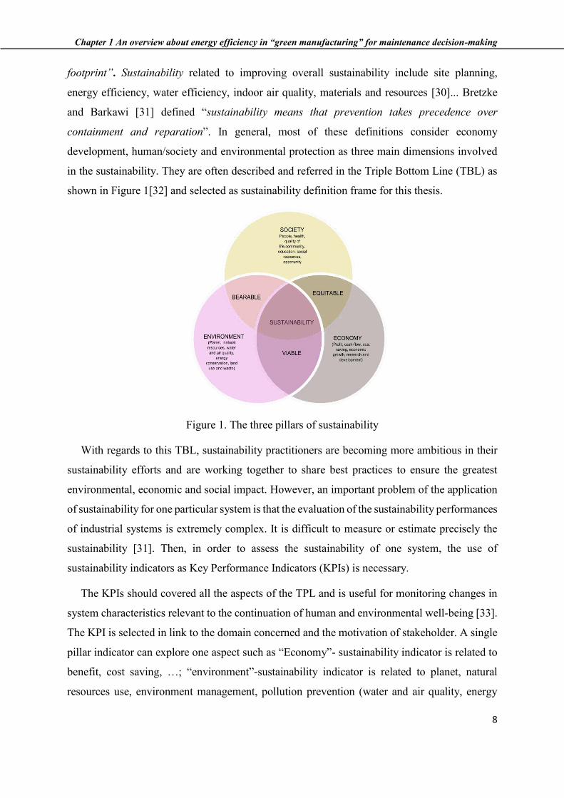
containment and reparation”. In general, most of these definitions consider economy
development, human/society and environmental protection as three main dimensions involved
in the sustainability. They are often described and referred in the Triple Bottom Line (TBL) as
shown in Figure 1[32] and selected as sustainability definition frame for this thesis.
Figure 1. The three pillars of sustainability
With regards to this TBL, sustainability practitioners are becoming more ambitious in their
sustainability efforts and are working together to share best practices to ensure the greatest
environmental, economic and social impact. However, an important problem of the application
of sustainability for one particular system is that the evaluation of the sustainability performances
of industrial systems is extremely complex. It is difficult to measure or estimate precisely the
sustainability [31]. Then, in order to assess the sustainability of one system, the use of
sustainability indicators as Key Performance Indicators (KPIs) is necessary.
The KPIs should covered all the aspects of the TPL and is useful for monitoring changes in
system characteristics relevant to the continuation of human and environmental well-being [33].
The KPI is selected in link to the domain concerned and the motivation of stakeholder. A single
pillar indicator can explore one aspect such as “Economy”- sustainability indicator is related to
benefit, cost saving, …; “environment”-sustainability indicator is related to planet, natural
resources use, environment management, pollution prevention (water and air quality, energy

Chapter 1 An overview about energy efficiency in “green manufacturing” for maintenance decision-making
9
conservation and land use); “Society”- sustainability indicator deals with people community,
education, equity, social resources, health, quality of life. Moreover, sustainability indicator, not
only in a single manner but in a more complex one, can be considered as a quantitative
aggregation of many indicators. It can provide a coherent, multidimensional view of a system
[2]. For example, energy intensity is seen as one of the important indicators for assessing two
pillars of sustainability (economy and environment) [34]. These aggregated indicators are very
useful for aiding stakeholders to identify the decision to be taken while supporting specific
sustainability interests [4]. Example of such indicators at the system scale is given in Table 1
[33].
Table 1. Proposed KPIs of sustainability for different classified scales and levels of system
These previous KPIs mentioned can be considered as general. Most of the time they should
be particularized to be well adapted to the domain, sector for which they have to be used (ex.
Finance, business, transport …). For example, in transport area, annual emissions of CO2,
passenger load factor, etc. can be selected as main KPIs of sustainability [35]. More precisely,
in industry (thesis context), companies are becoming more and more aware of the environmental
and social impact of their actions. Thus, a lot of focused KPIs can be addressed such as use of
recycled material, investments in environmental, life cycle footprint, CO2 emissions. This is
truer for the manufacturing domain considered as an industrial sector the most concerned with
Chapter 1 An overview about energy efficiency in “green manufacturing” for maintenance decision-making
10
the TBL requirements [18], [24], [36]. Effectively, sustainability in manufacturing is a very
important challenge and especially for Europe [37], [38]. It is one reason of the focus of this
thesis in manufacturing.
1.3. To sustainability in manufacturing industry: Green manufacturing
Manufacturing system can be defined as the arrangement and operation of machines,
equipment, people, material, people, control and information to produce usable products as
required by customers. Manufacturing system can consume different forms of energy input (e.g.
electricity, gas) to manufacture several classes of products (e.g. phone, laptop). Manufacturing
accounts for more than 30% of the global total energy consumption [37], [38], and it takes a
huge accounts for 16% of Europe’s gross domestic product (GDP) and remains a key driver for
innovation, productivity, growth and job creation. Manufacturing industry employs more than
32 million people in the EU and contributes about 75% of EU exports. However, manufacturing
enterprises are facing with a lot of advanced requirements from environment (new energy
resources, climate change, nature disaster), economic (e.g. short product life cycle, new
technologies) or social challenges (e.g. high living-standard, training skilled labor).
These requirements are supported by various drivers for sustainability in manufacturing such
as customer requirements with environmental regulation, energy crisis or rising trend of energy
and material prices. Strategies for Sustainable Industrial Development provided by World
Commission on Environment and Development [28] mentioned that “Resource and
environmental considerations must be integrated into the industrial planning and decision-
making processes of government and industry. This will allow a steady reduction in the energy
and resource content of future growth by increasing the efficiency of resource use, reducing
waste, and encouraging resource recovery and recycling”. So, it is a priority consideration on
sustainability for manufacturing plants. More precisely, sustainability in manufacturing means
“the production of products/services in such a way that it utilizes minimum natural resources
and produces safer, cleaner and environment-friendly products at an affordable cost or minimize
negative environmental impacts while preserving energy and natural resources” [4].
Sustainability manufacturing enhances the safety of employees, communities and products. For
example, Özşahin [39] indicated that a significant positive impact on environmental performance
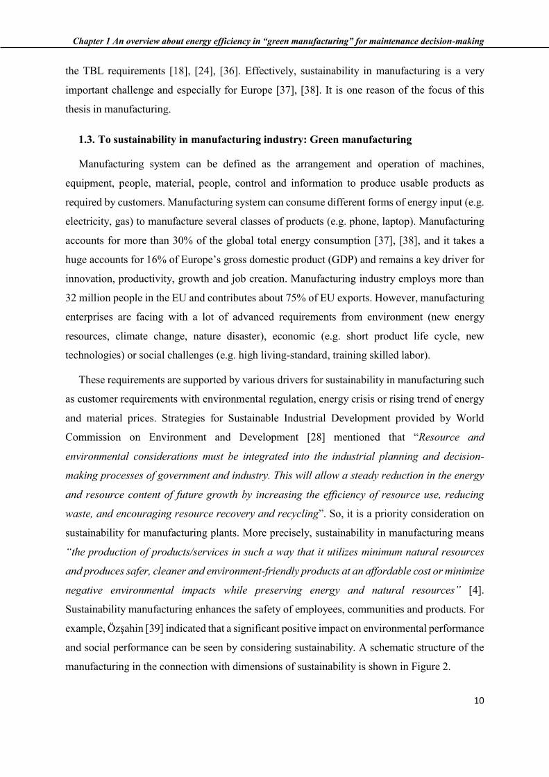
and social performance can be seen by considering sustainability. A schematic structure of the
manufacturing in the connection with dimensions of sustainability is shown in Figure 2.
Chapter 1 An overview about energy efficiency in “green manufacturing” for maintenance decision-making
11
Figure 2. Framework for Sustainable Manufacturing with the three pillars approach [40]
Under the impact of sustainability, EU launched the framework program on Research and
Innovation, for 2014-2020, “the Factories of the Future” (FoF) program. It is promoting
advanced characteristics for the future factories: cleaner, highly performing, environmental
friendly, and socially sustainable. Furthermore, “cleaner factory” makes production activities
more environmentally friendly by reducing/eliminating wasteful resources (i.e. less raw
material, water usage, and energy consumption). In that way, manufacturers respond to the rising
trend of demand for clean products/services that meet specific environmental, customer and cost
requirements. This advanced vision of manufacturing system takes into account really the TBL
together leading to adapt the plant structure, plant digitization, and plant processes. Indeed, the
plant structure of the future system has to comprise multidirectional layouts, with a modular line
setup and environmentally sustainable production processes (including efficient use of energy
and materials), well-interacting together and authorizing flexible production. For example,
dynamic arrangement of scheduled working will be more in phase with personal schedule
(including interchangeable machines and lines that can be reconfigured). This system evolution
promotes the development of manufacturing facilities that are more and more complex and
structured as multi abstraction levels in the way to make the solution emergent from the
interactions of all the components on these levels (e.g. hardware, software, human …). An
example of FoF interacted structure is shown in Figure 3 where a lot of digital technologies are
present (e.g. sensors, smart robots, the Internet of Things, big data and analytics). The
complexity of this plant is an advantage for being smarter, more adaptable to adjust the process
to its real operation conditions and the user needs. In that way, manufacturing stakeholders have
high ambitions to enhance their factories —85% of respondents believe they can benefit from
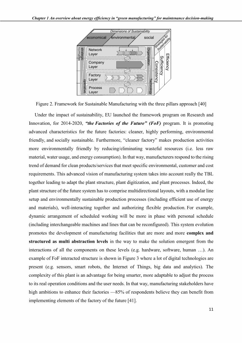
implementing elements of the factory of the future [41].
Chapter 1 An overview about energy efficiency in “green manufacturing” for maintenance decision-making
12
Figure 3. Future manufacturing system with the integration of IT system [41]
This global FoF orientation with regards to the TBL requirements leads to endorse “Green
manufacturing” or “Green production” concept to support “cleaner factory”. “Green
manufacturing” is defined in several research works [20], [21], such as : “Green manufacturing
is a sustainable approach to the design and engineering activities involved in product

Chapter 1 An overview about energy efficiency in “green manufacturing” for maintenance decision-making
13
development and/or system operation to minimize environmental impact”. “A green
manufacturing system, which involves reducing energy use, raw materials and solid waste,
reusing products, leads to production efficiency (i.e. less energy and water usage) [20]. Thus
“Green manufacturing” should avoid harmful waste, reduce hazardous emissions (CO2),
eliminate wasteful resources consumption, model the relationship between energy consumption
and other conditions [21].
In link to the previous definition, the KPIs usable in “green manufacturing” (and issued from
the list of those selected for industry area) are necessary covering the TBL frame. It can be
underlined the following KPIs:
- On environmental performance: air emission, water emission, … energy utilization, water
utilization, … solid waste, hazardous waste …
- On economic performance: product reliability, customer compliant …material cost, setup
cost … on time delivery, cycle-time … volume flexibility, product flexibility …
- On social performance: training and development, job satisfaction, … supplier
certification, supplier commitment …
These KPIs should be calculated at the different abstraction levels (e.g. components,
functions …) of the manufacturing system in accordance with decision-level addressed
(operational, tactical, and strategic). Indeed, these KPIs can serve to the different decision-
makers (e.g. operator, manager) and all along the system life-cycle, to take optimal decisions in
the frame of TBL requirements. This optimality is not easy to obtain because some of
sustainability requirements are antagonistic and difficult to be optimized as a whole. In that way,
the KPIs are integrated in different decision-making processes representative of all the system
life cycle phases (e.g. design, operation). One phase to be focused on is Maintenance because it is
proven that maintenance can impact and/or cover a lot of sustainable performances within “Green
manufacturing” (see Table 2) [42]. Among them, some works underlined [43]–[45], total energy
consumption, energy efficiency as key indicators [46].

Chapter 1 An overview about energy efficiency in “green manufacturing” for maintenance decision-making
14
Table 2. The proposed measures of sustainable maintenance performance measurement
systems
In fact, energy (in general) is as an important input for a system to produce external activity
or perform work required by any industrial process [47]. Energy usage is linked to social
development, economic development, environmental pollution and climate change. For
example, the energy cost for the total life-cycle of one industrial component can transcend capital
investment. In the case of an electrical motor, among the 100% total life-cycle cost, 2.5 % is
Chapter 1 An overview about energy efficiency in “green manufacturing” for maintenance decision-making
15
related to the purchase cost, 1.5 % is for maintenance and 96 % is the cost of energy used [48].
It leads to consider energy and its derivate materialization in terms of energy consumption and
product manufactured (useful output) as a main sustainability KPIs in manufacturing [39]
and more precisely “Green manufacturing”. Moreover, the ratio between energy consumption
and useful output can be represented with an Energy Efficiency value (EE). EE provides
substantial benefits in addition to energy cost savings, profitability, production and product
quality, and improving the working environment while also reducing costs for operation and
maintenance, and for environmental compliance [49], [50]. For example, EU established
motivated targets towards industry: a 20% energy savings target by 2020 and moving towards
a 20% increase in Energy Efficiency. Thus EE seems an important target for sustainability in
manufacturing and more precisely with regards to maintenance decision-making process.
1.4. What is energy efficiency in general … and then in industry?
1.4.1. Energy efficiency in general
EE is an universal concept mentioned in various applications and known under various names
like energy intensity [51], [52], specific energy consumption [53]–[55], energy conservation
[56]. Indeed, the definition of energy efficiency is a complex issue. Generally, energy efficiency
means more concretely that a smaller amount of energy input is needed for the same useful
produced output/services, or that a higher output/services may be provided with the same energy
input. For example, single crystalline photovoltaic panel can produce more electrical energy than
thin-film photovoltaic panel with the same incident solar power. So saving energy or reduction
of energy consumption are well-known behaviors of EE such as replace incandescent bulbs by
florescent lamp.
The relationship of EE with economic, social behaviors or environmental issues have been
already analyzed over the past decades [57], [58]. It is due to the interests to be energy-efficiency
with increase in demand for energy, rising energy, materials prices, changing consuming
behavior of customers to be green … together with the growing environmental concerns. There
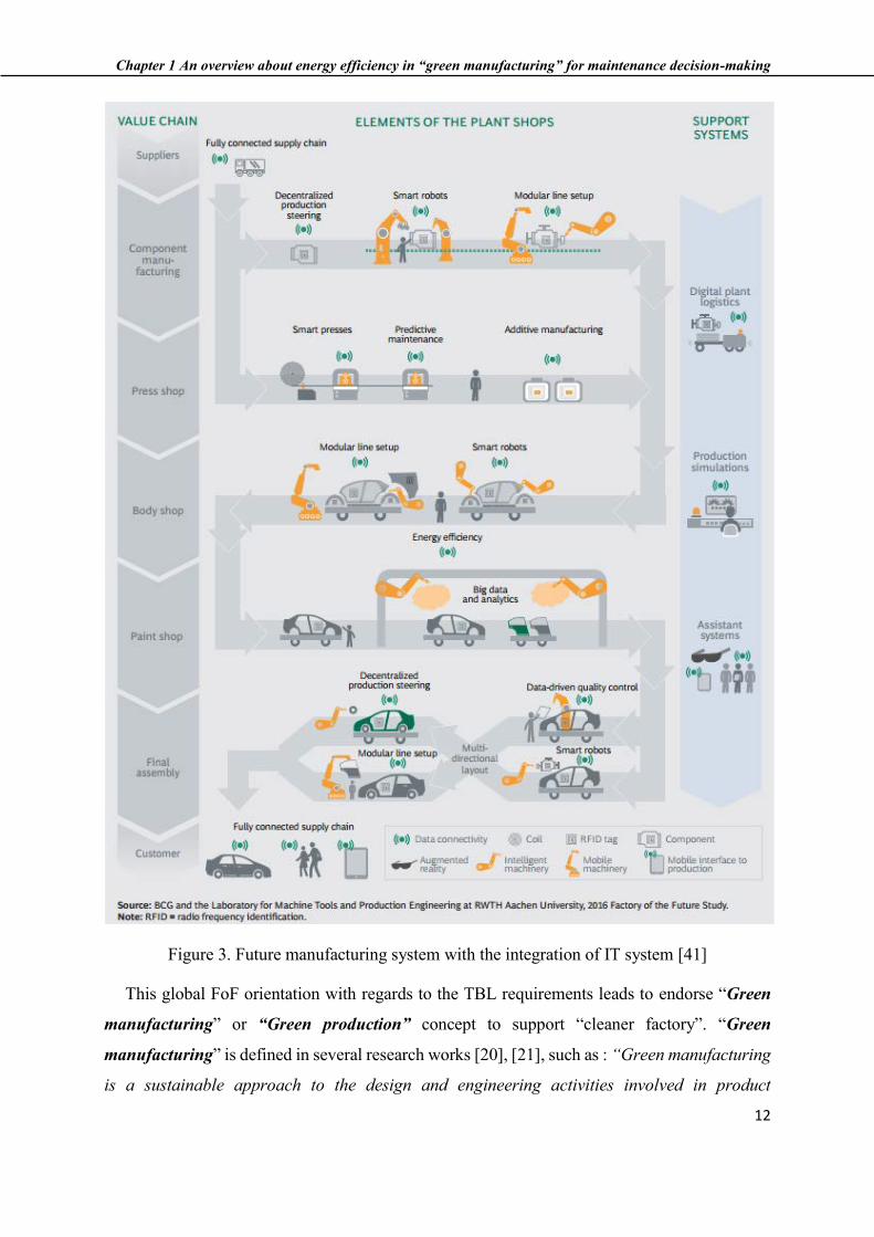
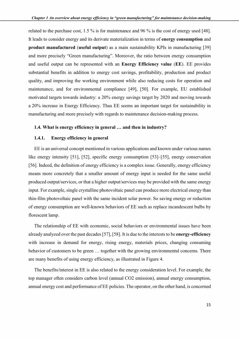
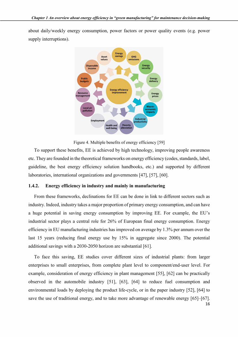
are many benefits of using energy efficiency, as illustrated in Figure 4.
The benefits/interest in EE is also related to the energy consideration level. For example, the
top manager often considers carbon level (annual CO2 emission), annual energy consumption,
annual energy cost and performance of EE policies. The operator, on the other hand, is concerned
Chapter 1 An overview about energy efficiency in “green manufacturing” for maintenance decision-making
16
about daily/weekly energy consumption, power factors or power quality events (e.g. power
supply interruptions).
Figure 4. Multiple benefits of energy efficiency [59]
To support these benefits, EE is achieved by high technology, improving people awareness
etc. They are founded in the theoretical frameworks on energy efficiency (codes, standards, label,
guideline, the best energy efficiency solution handbooks, etc.) and supported by different
laboratories, international organizations and governments [47], [57], [60].
1.4.2. Energy efficiency in industry and mainly in manufacturing
From these frameworks, declinations for EE can be done in link to different sectors such as
industry. Indeed, industry takes a major proportion of primary energy consumption, and can have
a huge potential in saving energy consumption by improving EE. For example, the EU’s
industrial sector plays a central role for 26% of European final energy consumption. Energy
efficiency in EU manufacturing industries has improved on average by 1.3% per annum over the
last 15 years (reducing final energy use by 15% in aggregate since 2000). The potential
additional savings with a 2030-2050 horizon are substantial [61].
To face this saving, EE studies cover different sizes of industrial plants: from larger
enterprises to small enterprises, from complete plant level to component/end-user level. For
example, consideration of energy efficiency in plant management [55], [62] can be practically
observed in the automobile industry [51], [63], [64] to reduce fuel consumption and
environmental loads by deploying the product life-cycle, or in the paper industry [52], [64] to
save the use of traditional energy, and to take more advantage of renewable energy [65]–[67].

Chapter 1 An overview about energy efficiency in “green manufacturing” for maintenance decision-making
17
Thus, the energy efficiency understanding can vary with industrial domain and type of used
energy [22], [23]. It leads to consider EE under different forms like thermal energy efficiency
[68], economic ratios, techno-economic ratios [69], energy intensity or energy efficiency
intensity [70], [71], Energy Efficiency Design Index [72], or benchmarks for energy efficiency
[73], fuel economy [74], [75]…
These EE forms for which understanding of EE properties is increasingly important [50], are
also considered in manufacturing domain because EE is shown as a way to increase the
competitiveness of manufacturing system [51], [69], [76]. It is illustrated in the sustainable
manufacturing framework given in Figure 5 [62] for contributing to the TBL. Indeed, during
recent years, energy consumption of manufacturing industry domain has achieved a rapid
growth. International Energy Agency (IEA) presented in energy efficiency market report that
over 23 % of global energy consumption is consumed by manufacturing industry [38], [75]. It
takes the second place in the energy and emission by end users according to the same IEA’s
report. Moreover, manufacturing is continuously expanding with huge investment and rapidly
increase in facilities to supply the demand of good/services for modern life [77]. It leads to
integrate EE in the Energy Management System (EMS), which was recently implemented, to
help managers master their system [78], [79]. EMSs with energy monitoring systems
(online/offline, continuous or energy audit, etc. ) have been proposed and successfully been
applied in different types of manufacturing system [80]–[82]. In that way, optimization of EE in
manufacturing with regards to the other KPIs is appearing as a main challenge for decision-
makers.
Figure 5. EE contributing to TBL of sustainable manufacturing frameworks [62]
Nevertheless, few works already exist on EE in decision-making process. For example,
Trianni [83] studied the benefit of EE in both decision-makers and policy-makers. In fact,

Chapter 1 An overview about energy efficiency in “green manufacturing” for maintenance decision-making
18
industrial system such as manufacturing one has to face with a set of stakeholders, including
decision-makers, energy providers, end-users and operators interacting at different layers
according to their roles, and in consist with the decision/action levels to be addressed (e.g.
operational, tactical or strategic levels) [71], [84], [85]. At the operational level, the issue should
be: How the energy consumption and thus the energy efficiency of machines and production
systems have to be materialized to give the right decision as soon as possible (nearly real time)
[85]? In another way, at higher level (tactical or strategic levels) only energy consumption is
used to modify the usage of different types of energy resources.
Whatever the level addressed, the EE is mainly assessed by a value. It is represented by the
EE Indicator, named EEI, as an index for evaluating the energy efficiency at a specific time.
However, no generic formulation of this indicator is available today in the manufacturing field
to be applicable to the different abstraction levels. Indeed, even if some methods to assess EEI
exist, they are addressing principally EEI values at the component level without considering
really it at the system one which can be better for performance optimization [5], [6]. Moreover,
this assessment is not easy to do because it should take into account the dynamics of the system
(age, degradation, different loading profiles, etc.) impacting the EEI value and leading to track
its evolution in the future to clearly define the Energy Efficiency Performance (EEP). The EE
Performance is a performance materializing if the industrial system is efficient or not (it is more
than a value; it is the value in time). However, today, most of the studies on EEP considers that
EEP (through EEI) is time-independent [86], [87]. Predicting the degradation behavior of energy
efficiency of components/systems is therefore crucial [88], [89] in order to anticipate the increase
in global energy consumption, improve opportunities to save energy, etc. So, the consistent
formulation of these EEI and EEP items is not evident [7] especially with regards to dynamic
context (dynamics of the systems) for predicting the EE evolution in the same way as it was
done through the use of conventional prognostics approaches to predict the Remaining Useful
Life (RUL) of components/systems [8]–[11].
Thus, in summary with the EEI/EEP consideration in green manufacturing, the first important
challenge addressed in the thesis is:
How to define and evaluate/predict EEI/EEP at the different abstraction levels of an
industrial (manufacturing) system by considering the dynamics of this system? - Challenges
No.1
Chapter 1 An overview about energy efficiency in “green manufacturing” for maintenance decision-making
19
The results of these formalizations should be integrated in the decision making processes of
the manufacturing system to master the EEI/EEP as close as possible to its nominal value for
controlling Environmental Pillar. More precisely this mastering requirement can be supported
by the maintenance decision-making process as advocated the Prognostics and Health
Management (PHM) community [12]–[14]. Indeed, an efficient maintenance strategy could not
only avoid the failure of the system but also allow to anticipate the growing up of global energy
consumption. Nevertheless, the current maintenance decisions are mainly based on conventional
indicators such as reliability, availability, direct cost, etc. [15] and only just some investigations
have been realized to consider the relationships between EEI and maintenance strategy [16],
[17]. For example, Xu and Cao [16] addressed the average energy efficiency under periodic
maintenance as a criterial criteria for the maintenance decision making process at machine level
only.
This relationship between conventional indicators and sustainable ones for maintenance
opens up a new path to define/adapt the “condition” to trigger the maintenance (CBM one)
according to sustainability requirements and the evolution of their values (to promote originality
towards EEP).
1.5. How to integrate EEI/EEP in maintenance decision-making and more precisely in
CBM?
Maintenance is defined as “combination of all technical, administrative and managerial
actions during the life cycle of an item (e.g. component, machine) intended to retain it in, or
restore it to, a state in which it can perform the required function” [90]. This combination leads
to support different strategies depending if the item is already failed (corrective strategies) or not
(preventive strategies) [91], [92]. However, the question of how EE helps or impacts these
strategies is only in investigation.
1.5.1. Classification of maintenance strategies
Maintenance strategies are implemented with regards to strategic decision (after or before
failure) and by organizing all the activities to support this decision execution (e.g. management,
planning). So, maintenance strategies have been chosen either on the basis of longtime
experience or by following the recommendations of manuals provided by manufacturers [93]
such as original equipment manufacturer (OEM) recommendations. There are classified, as

Chapter 1 An overview about energy efficiency in “green manufacturing” for maintenance decision-making
20
presented in Figure 6. in two main categories: corrective maintenance and preventive
maintenance [90], [94]–[96].
Corrective maintenance: It includes all the maintenance activities that are carried out after
fault recognition and intended to put an item into a state in which it can perform a required
function [97], [98]. For example, corrective action is necessary when the system is failed but
could be investigated when the component is not critical both on the direct and indirect costs
(e.g. low cost components) [45]. In some other cases, when the indirect cost is high, corrective
maintenance should be avoided as much as possible.
Indeed, costs can be classified as direct costs and indirect costs based in the way they
contributed to the objective of manufacturing system [45]. The direct costs are directly related
to all the “resources” needed to develop the maintenance actions. Indirect costs are more the
costs concerned by the impacts of the fact that the system is stopped (for developing the
maintenance action for example after corrective situation) or that the maintenance action is not
done keeping the system as degraded (non-optimal performance situation).
Corrective maintenance can be declined in palliative maintenance (e.g. Maintenance action
to recover a part of the performances as it was before the failure) or in curative maintenance (e.g.
change the failed component to be As Good As New after the action).
Preventive maintenance: Maintenance carried out at predetermined intervals or according to
prescribed criteria and intended to reduce/prevent or delay the probability of failure or the
degradation of the functioning of an item (reducing the number and cost of failure of an item,
increasing system reliability, improving availability equipment, ensure the security of
individuals and the environment, facilitate inventory management, etc.) [97]–[99]. Preventive
maintenance makes sure that maintenance is performed before failure occurs to avoid corrective
maintenance actions. Preventive maintenance may be either scheduled maintenance,
predetermined maintenance or condition based maintenance (CBM).

Chapter 1 An overview about energy efficiency in “green manufacturing” for maintenance decision-making
21
Figure 6: Simplified classification of maintenance strategies
Scheduled maintenance (Time-based or planned maintenance): Preventive maintenance
which is carried out in accordance with an established time schedule or established number of
units of use. It leads to develop potentially actions too “soon” or too “late”.
Predetermined maintenance (Age-based maintenance): Preventive maintenance carried out in
accordance with established intervals of time or number of units of use but without previous
condition investigation. Substantial remaining useful life is wasted if the machine is still in
reasonable condition when preventive maintenance is performed, and a breakdown might occur
if it happens to deteriorate faster than expected [100].
Condition Based Maintenance (CBM): Preventive maintenance which is based on
performance and/or parameter monitoring and the subsequent actions. The monitoring of
performance and parameter, called “condition”, may be scheduled, on request or continuous
(e.g. real time monitoring). Thus, it includes a combination of condition monitoring and/or
inspection and/or testing, analysis and the ensuing maintenance actions. An extension of CBM
is called Predictive Maintenance which is corresponding to a CBM carried out following a
forecast derived from the analysis and evaluation of the significant parameters of the degradation
of the item. CBM also considers external, random failures (for example, shock, natural disasters,
humans mistakes) [101].
The principle of CBM is therefore to perform maintenance action by anticipating causes
before the failure occurs in order to avoid the effects of unexpected failures. The anticipation is
related to the tracking of degradation level of the condition (degradation indicator). As the
condition can be parameter or performance, the tracking of this degradation can be directly on a
raw signal, an information (resulting from signal processing), an indicator (resulting from
information fusion), a health state (resulting from indicator fusion) as advocated by PHM
Chapter 1 An overview about energy efficiency in “green manufacturing” for maintenance decision-making
22
community ... The indicator has to be compared to a threshold representing the limit of the value
considered as acceptable. Then, this degradation indicator is used as input of the maintenance
decision-making process. In that way, CBM is really examined by industry to be more just in
time in maintenance. For example, the vibration and temperature of the mechanical component
such as bearings and gears or the current and voltage provide the “condition” of an electric motor
[94]. Deterioration process due to tear of belt-driven system [102], [103], wear of cutting [104],
[105], crack of rolling part [106], [107] may be selected as “deterioration” condition for CBM.
Hazards could be also considered as a condition for CBM strategy [108].
Through this notion of “condition”, CBM seems the best strategy to be investigated to trigger
the maintenance action according to sustainability requirements and the evolution of their values
(in terms of degradation impact; EEI then EEP). The value is going up to the threshold. Indeed,
tracking a conventional indicator or a sustainable one could use the same techniques and brings
similar advantages.
In terms of advantages, the CBM, implemented through different ICT products (e.g. sensors,
networks, software …) can extend equipment life (age), reduce risk and improve the efficiency
of equipment [109]. CBM can also indirectly contribute to optimisation of the production process
(e.g. better mastering of product quality) [95], minimizing costs of maintenance [45].
The general decision-making process for CBM deployment is synthesized in Figure 7. It is
consistent with standards to help engineer for developing particular CBM platform/architecture
related to the system to be maintained. The main well-known standard is the OSA-CBM (Open
Systems Architecture for Condition-Based Maintenance) [45], [110]. The OSA-CBM
architecture is structured on 6 processes to carry out the action from the data acquired: Data
Acquisition, Data Manipulation, State Detection, Health Assessment, Prognostics Assessment
and Advisory Generation.
More precisely, by taking into account the result of the health assessment process in terms of
advanced information about the system operation (including production plans, logistics
schedule, resourses avaiable …), the prognosis allows to track the future state of the system
[111]. It is more true now in the more recent CBM studies [112]–[114] while considering not
only condition at current time but also in the realistic operating conditions of the system over
time (in the future).

Chapter 1 An overview about energy efficiency in “green manufacturing” for maintenance decision-making
23
However, the main issue on CBM is related to the identification of the most suitable
“condition” (indicator) and how to master/evaluate this indicator to use it as input of the decision-
making process (with regards to the threshold fixed). Indeed, the methods/tools to select and
support “condition” indicator evaluation, and threshold fixing are not completely available. It is
necessary to find methodologies usable with regards to the complexity of the system targeted,
its main properties to be monitored (e.g. performances, parameters) and to the decisions to be
taken in an optimal way. More precisely, optimal maintenance decisions for a complex system
are not necessarily obtained by the superposition of individual decisions found at each level of
the system.
Figure 7. Structure of CBM decision-making [109]
This superposition in the decision is all the truer by considering both types of indicators,
conventional and sustainable one such as EEI/EEP. Sustainability consideration in CBM means
for example: When an item (component/system) consumes more energy, it should be replaced
even if it is not degraded with regards to other properties such as wear. In that way, maintenance
of the component could be realized to preserve its energy property [87], [115]. It is an original
way for developing maintenance.
1.5.2. Is Energy Efficiency already integrated in maintenance and mainly CBM?
Only few works on the impact of maintenance on the EEI/EEP (mostly amount of energy
saving or energy consumption) already exist in industrial area. For example, Yildirim and
Nezami [116] studied energy consumption model under the impact of minimal repair and
potential recovered EE after implementing maintenance as computed by using efficiency curve.
Chapter 1 An overview about energy efficiency in “green manufacturing” for maintenance decision-making
24
The developed cost model shown that better cost benefits can be achieved by considering the
energy consumption of production process to decide the maintenance actions. These benefits can
be results of a low energy inspection cost (by investment in energy monitoring system) or the
balance between maintenance cost and energy cost. Mora et al. [7] mentioned EE as a trigger of
preventive maintenance actions, and take into account energy cost in comparison with the
preventive maintenance cost for maintenance decision making process. These previous works
are mainly related to scheduled or predetermined maintenance strategies. Indeed, CBM
strategies are not really addressing EE properties. EE is seen only as the auxiliary result of these
previous CBM plans. For example, Sánchez and Goti [117], [118] investigate the preventive
maintenance scheduling problem in a production system where maintenance is impacting the
production speed and quality. They show production speed and output quality decrease as a
function of machine deterioration [119] and optimized energy consumption can be reflected in
many maintenance schedules. The impact of maintenance and operating procedures (at
function/system level) into energy model to calculate energy consumption is addressed, then
energy saving is the objective of maintenance plan instead of conventional indicators for
maintenance decision making process [17]. Optimization framework can provide enhanced
decision support leading to optimal operation and maintenance [120]. Nevertheless, these works
are not really developed by integrating EEI/EEP as concrete conditions to be tracked for aiding
the maintenance decision process. It leads to identify the second important challenge addressed
in the thesis which is:
How to use EE into CBM strategies? - Challenges No.2
This challenge placed the main originality of the thesis by considering EEI/EEP as conditions
to trigger suitable maintenance action, which allows not only to avoid the failure of the industrial
component/system but also to maintain the EEI/EEP. In that sense, the degradation indicator in
the thesis is considered as a quantified indicator directly related to the state of degradation or
performance of an item (component, machine, system) from which it is possible to detect a
failure.
1.6. Conclusions
This chapter presented the sustainability context of this thesis. It is more focused on
sustainability in “Green Manufacturing” by considering the requirements of some initiatives
such as FoF (advanced manufacturing) in which it is advocated “cleaner factory” as a necessary
Chapter 1 An overview about energy efficiency in “green manufacturing” for maintenance decision-making
25
way for the future generation. Among the KPIs representative of the TBL of this factory type,
Energy Efficiency (EE) was identified as the main important one. It allowed to underline EE
Indicator (EE value at t time) and EE Performance (evolution of the EE value in time according
to dynamics of the system) as two items must be necessarily mastered at each level of the
manufacturing system to gain the green property.
The results of this mastering should be integrated in the maintenance decision-making process
(mainly CBM one) of the manufacturing system to control the EEI/EEP as close as possible on
its nominal value. Nevertheless, current maintenance strategies are not well adapted to support
this integration because mainly based on conventional indicators and not sustainable ones.
Therefore, with regards to the two conclusions on EEI/EEP mastering and its integration in
maintenance/CBM strategy, the chapter highlighted two main challenges to be addressed in the
thesis:
- How to define and evaluate/predict EEI/EEP at the different abstraction levels of an
industrial (manufacturing) system by considering the dynamics of this system?
- How to use EE in CBM strategies?
These two challenges serve in chapter 2 to define the scientific issues to be attacked.

Chapter 1 An overview about energy efficiency in “green manufacturing” for maintenance decision-making
26
Chapter 2 Scientific problem statement on EE concept and its application in CBM maintenance decision-making
27
Chapter 2 Scientific problem statement on EE concept and its application in CBM maintenance decision-making
2.1 Introduction
The chapter 2 aims to define the scientific issues which are related to the two identified
industrial challenges of chapter 1. In that way, the chapter 2 starts from challenge 1 with the
consideration of using EE in general in order to underline the categories to develop EEI concept
at multi-levels of a manufacturing system. Then it is investigated generic EEI formulation taking
into account the common characteristics of manufacturing system (complex, multi-level
structure, dynamic context). From this EEI formulation, the time-dependent factors are
considered to track EEI evolution to introduce EEP. It allows to focus on EEP as the estimation
of the residual life energy at different levels of manufacturing system. After that, the dynamics
of the system and its relationship with prognostic are investigated. It enables to isolate the
interest of a generic approach to predict EEI evolution and estimate EEP by applying suitable
prognostics. Finally, with regard to challenge 2, an investigation is done about innovation on
maintenance decision-making (focus on CBM) by trigger maintenance actions not only by using
conventional conditions but also EEI/EEP ones.
2.2 How to define and evaluate/predict EEI/EEP at the different abstraction levels of an
industrial (manufacturing) system by considering the dynamics of this system?
In link to the first challenge defined in chapter 1, it is important to focus first on EEI concept
(see section 2.2.1), then its consideration at multi-levels of a manufacturing system (see section
2.2.2), and finally on the EEP concept (see section 2.2.3) as an aspect of EEI evolution with the
consideration of the system dynamics (see section 2.2.4).
2.2.1 General concepts of EEI and their application in manufacturing systems
Over the past decades, many governments and industrialists have focused on energy
efficiency (EE) assessment as a powerful tool for decision-making. Indeed, this assessment
should lead to strategic decisions and priority actions for reducing energy consumption, energy
demand and environmental problems. For this assessment, EE is generally expressed as using
Chapter 2 Scientific problem statement on EE concept and its application in CBM maintenance decision-making
28
less energy to produce the same amount of services or useful outputs. In that way, EE equation
is most of the time formulated as: Useful output of a process
Energy input into a process[121]. It means that a smaller amount
of energy input is needed for the same useful produced output, or that a higher output is provided
with the same energy input. In this way, energy efficiency can be used in a very wide range of
applications and for different levels of features [122] in terms of energy demand sectors (e.g.
buildings, appliances, transports, industries, services, etc.), sizes (e.g. on a local, national,
international or global scopes), stakeholders (e.g. decision-makers, energy providers, end-users,
energy services companies, energy audit services companies, or particular equipment). For
example, EE has already been investigated in several sectors such as industries [51], [64],
transport [63], [123], and buildings [124], [125]. Nevertheless, for each sector [55], [87],
different visions of EEI concept have been introduced but it is globally accepted that these
visions belong to four categories to design EEI [57], [126].
1- Thermodynamic indicators: They are measured as the energy dissipated or
consumed by the system compared to the amount of energy in the resource processed. Both
input and output are measured in thermodynamic units (e.g., GJ (Gigajoules) of delivered
energy consumed in the production coke for coking coal). The importance of efficiency
comes from the thermodynamic laws, namely the conservation of energy and the irreversible
energy conversion to uselessness. By decreasing the energy loss in the processing, the useful
energy transformed from energy input is increased. Thus, the thermodynamic definition of
energy efficiency can be expressed as follows: 𝑈𝑠𝑒𝑓𝑢𝑙 𝑤𝑜𝑟𝑘 𝑜𝑟 𝑒𝑛𝑒𝑟𝑔𝑦 𝑜𝑢𝑡𝑝𝑢𝑡
𝐸𝑛𝑒𝑟𝑔𝑦 𝑖𝑛𝑝𝑢𝑡 [127]. Based on
this definition, this type of indicators should not be applied to unknown thermodynamic
characteristics or to the case in which there is no or poorly-monitored process because of
missing information about energy loss. Relatively, thermodynamic indicators are not the best
choice at the top level of national and international energy. Indeed, using this type of EEI,
energy efficiency presents changing trend (improvements/decrements) of several energy
conversion facilities. It can be underlined such as the promising conversion efficiencies to
convert sunlight into electricity energy. It can reach to maximum 44.3% of conversion and
depend on the types of PV panel [128]. According to [129], thermodynamic energy efficiency
can be used only at the device level, end-use technology or energy conversion technology.
2- Physical-thermodynamic indicators: This kind of indicators has been introduced
to avoid the limit of thermodynamic indicators in systems with output units that are

Chapter 2 Scientific problem statement on EE concept and its application in CBM maintenance decision-making
29
uncountable or specific energy format like systems in transport or agriculture. In fact, the
output is evaluated in physical units while the input is in energy. In this way, the energy
efficiency can be evaluated as follows: 𝑈𝑠𝑒𝑓𝑢𝑙 𝑝ℎ𝑦𝑠𝑖𝑐𝑎𝑙 𝑜𝑢𝑡𝑝𝑢𝑡
𝐸𝑛𝑒𝑟𝑔𝑦 𝑖𝑛𝑝𝑢𝑡 level [126], [130], [131]. It is
important to note that the units of physical output have to be expressed in the designed units
of the system capacity (tons of cement, passengers, kilometers, vehicles, the number of
rooms, etc.). Calculated in either aggregated or disaggregated methods, these indicators
directly stick to the technical power flow. As a consequence of various physical outputs,
multiple forms are used for physical-based indicators such as energy intensities, specific
energy consumption, etc. In spite of difficulties in quantifying the higher level of aggregated
process, the physical-thermodynamic indicators can be applied to a variety of levels ranging
from a very simple component level to a sector level [132].
3- Economic-thermodynamic indicators: These indicators are hybrid indicators, in
which the energy input is measured in thermodynamic units and the output is measured in
market prices ($). The market prices are measured by the GDP or the market value of all final
goods and services produced within a country or a sector [121], [131]. In this case, any
difference in the output or input number can be affiliated to economic, social behaviors or
calculation methods. The information of technical process is unnecessary and the energy
output number is conveyed through energy price factors. The “Energy:GDP” increments may
be misunderstood as the positive result of energy efficiency investment. But economic-
thermodynamic indicators can be calculated by multiplying thermodynamic indicators with
the economic value of output units. Thus, these indicators can be applied to high levels of
economic structures such as the corporate, sub-sector, sector and national levels.
4- Economic indicators or monetary indicators: These indicators are used to
measure changes in energy efficiency purely in terms of market values. They are named as
the energy to GDP ratio, energy coefficient or energy elasticity. Economic indicators are
given as the ratio of energy consumption in an energy unit to an economic activity in a
monetary unit 𝐷𝑜𝑙𝑙𝑎𝑟𝑖𝑧𝑒𝑑 𝑜𝑓 𝑜𝑢𝑡𝑝𝑢𝑡
𝐷𝑜𝑙𝑙𝑎𝑟𝑖𝑧𝑒𝑑 𝑜𝑓 𝑖𝑛𝑝𝑢𝑡 [47], [48]. Sometime, these indicators are convertible from
their physical-thermodynamic indicator counterparts by simply multiplying the energy input
with appropriated added energy prices. But, in another way, these economic indicators are
just seen as a purely economic efficiency indicator rather than as an EEI because they are
fully measured in economic values. This type of indicators should not be used in monitoring
Chapter 2 Scientific problem statement on EE concept and its application in CBM maintenance decision-making
30
energy efficiency performance systems. The economic indicators are often used when energy
efficiency is measured at a high level of aggregation (international, national and sector levels),
where it is impossible to characterize the output by a single physical unit.
In conclusion, some of these categories of EEI are limited to the physical evaluation of energy
transformations, while others also consider the economic and social dimensions that define the
usefulness of a process [133]. The consideration of these dimensions for EEI is mandatory in the
frame of TBL as advocated by Manufacturing system and more precisely “Green
manufacturing”.
Indeed, as already explained in chapter 1, the manufacturing system under the orientation of
FoF (more “cleaner factory” property) is mainly characterized by:
(i) The energy consumed which can be represented by different forms (e.g. electricity,
gas, oil),
(ii) The outputs produced which can be materialized by different products or classes of
products due to the flexibility/adaptability of the system (e.g. a same assembly line
can assemble different parts to form different final products),
(iii) The structure which is complex and organized on multi abstraction levels.
Thus, these characteristics have to be taken into account to select which one of the EEI
categories is the most adapted to manufacturing system. In that way, the next table is showing
the main advantages and disadvantages about the use of these categories in manufacturing
system [69].

Chapter 2 Scientific problem statement on EE concept and its application in CBM maintenance decision-making
31
Table 3. The advantages and disadvantages of the categories of EEI to be applied in
manufacturing systems [69]
Primary Advantages Primary Disadvantages
Thermodynamic
Energy Efficiency
=Useful work or energy output
Energy Input
- Different forms of energy inputs is converted to common form.
- Hidden energy in output is not the most concern of manufacturing system.
- Thermodynamic laws are not easy to use for calculating the energy losses for all machines/component of manufacturing system.
Physical-Thermodynamic
Energy Efficiency
=Useful (Physical) Output
Energy Input
- Physical measures for the output(s) can be determined and mastered during manufacturing process.
- EEI can be defined individually for multiple functions (with different outputs) within the same manufacturing system.
- Difficulty to evaluate the energy input allocated for different types of outputs.
Economic-Thermodynamic
Energy Efficiency
=Dollarized Output
Energy Input
- The aggregation of several forms of manufactured outputs can be calculated by assigning market prices.
- EEI is influenced by other economic factors.
- The changing of EEI value is not representative of the system structure modification and without possibility to locate the technical causes of EEI changing.
Economic-Economic
Energy Productivity
=Dollarized Output
Dollarized Energy Input
- EEI of different manufacturing systems can be compared and aggregated at various levels.
- EEI is influenced by other economic factors.
- The changing of EEI value is not representative of the system structure modification and without possibility to locate the technical causes of EEI changing.
This previous positioning about the four EEI categories with regards to manufacturing system
underlines that any specific category is supporting the main characteristics defined for this type

Chapter 2 Scientific problem statement on EE concept and its application in CBM maintenance decision-making
32
of system [68]. So, a first scientific need is to clearly define the EEI in the context of
manufacturing system and more precisely “Green manufacturing” as defended by FoF
initiative.
2.2.2 EEI at each level of abstraction (component, function/system) of a manufacturing
system
This scientific need is all the truer since the EEI formulation to be found must be applicable
to the different abstractions level of a manufacturing system (the third characteristics
mentioned previously).
Indeed, such system has to be faced with a set of stakeholders, including decision-makers,
energy providers, end-users and operators [71], [84] interacting at different abstraction levels
according to their roles, and in consistency with the decision/action levels to be addressed (e.g.
operational, tactical or strategic levels). Moreover, this level consideration implies also to
retrieve data on energy consumption (e.g. kWh, Btu, ton of coal) and output unit (e.g. amount of
manufactured cars) consumed and produced at each level, knowing that there is often limited
resources (financial, labor, instrument, etc.) for collecting this necessary data. Thus, one
challenge is to found, in an optimal way, what is the EEI the most applicable at each level by
considering also the retrieval of the data. In relation to this challenge, the Table 4 is providing a
first illustration on the relationships between EEI and application level in manufacturing area in
order to give to the decision-maker some helps for selecting the best EEI [1].
This table highlights the potential availability of EEI at each level of manufacturing system
(and its enterprise context). Nevertheless, these EEI are positioned in an isolated way (each one
is issued from a specific work) without introducing rules for developing one EEI at a specific
level from EEI at another lower level (e.g. aggregation principle). Indeed, for example, some
existing works focus on EEI at component level (i.e. operational layer) [134]–[136] without
considering it at higher level (i.e. the strategic layer) which may be useful even essential for
optimizing decision-making process [137], [138].

Chapter 2 Scientific problem statement on EE concept and its application in CBM maintenance decision-making
33
Table 4. Consideration of EE concepts at different levels of manufacturing
Reference EE indicator Level of application in manufacturing area
[16] Energy consumption Physical-thermodynamic indicators
Component/equipment
[25] Energy efficiency label Factory level Department level Unit process level
[57] Physical-thermodynamic indicators Thermodynamic indicators
All levels of manufacturing process
[62] KPIs Benchmarks
Country level Sector level Plant level
[120] Energy consumption Function/system level [139] Thermodynamic indicators
Physical-thermodynamic indicators
All levels of manufacturing system
Economic-Thermodynamic indicators Factory level Sub-sector/sector level Industrial sector level Country level
[140] Physical-thermodynamic indicators Function/system level [141] Physical-thermodynamic indicators Machine level
According to this separation highlighting (component/system), most of the time the EEI at
component level, is based only on the measurement of its energy consumption and its output
with the consideration of several impact factors/features associated with individual components
like temperature, voltages and harmonics. Thus, EEI value at this component level can be
directly measured. For example for an electrical motor, its EEI is based on the energy
consumption and produced mechanical energy taking into account several parameters (e.g.
speed, frequency of harmonics) [142]–[144].
At the system level, EEI should be representative not only of the components which are inside
this system (different components place in series and/or parallel) but also of the global behavior
of this system which is resulting from the components interactions and the operational
conditions. This global behavior can be impacted by the service of the system which is depending
of the outputs to be delivered (e.g. a same system can support different services in link to its
adaptability/flexibility level). So, the EEI assessment at this level is not easy to do due to this
dynamic consideration impacting necessary energy consumption characteristics[145]. About
Chapter 2 Scientific problem statement on EE concept and its application in CBM maintenance decision-making
34
system level, Behrendt [146] argued that the largest energy efficiency potential belongs to the
higher system levels. He developped an EEI model based on the three levels of industrial electric
motor-driven system, including operational conditions and human aspects. This model is
comprising the components behaviors, the interactions between them, but also the behavior of
the whole system regarding to the service to be achieved.
Thus, the interactions between the components identified by their own EEI, in the way to
deliver the EEI at the system level have to be clearly understood. It is materializing the required
step from component/system separation to component/system integration. Indeed, both energy
consumption and output (the two main properties of EEI) at component level should be used to
calculate EEI at function/system level. However, these interactions are representative of a
complexity not so easy to understand. For example, the energy consumed by a component may
be transformed to energy to be consumed by another one … with some energy loss due to the
transformation (e.g. air compressor transforms electricity to air pressure for another component).
The same situation exists with output of one component, which may be reused as input of other
component. Through these transformations and the resulting losses, it becomes clear that the
energy consumption model at system level (suitable to provide the basis for the energy optimal
use of manufacturing plants) cannot be based only on the sum of the individual components
[147], [148] but must integrate the energy consequences of the component interactions.
In addition, EEI assessment both at component and/or system levels needs also to consider
some factors which are impacting their properties (energy consumption and output) [148] [149].
Indeed, EEI is influenced by several factors such as the system age/degradation, the type of
energy resources (coal, fuel, electricity), the technology employed for controlling EE [150] ...
These factors are representative both of internal parameters or events to the component/system
(e.g. machine speed, energetic profile) [141], but also external parameters or events to the
component/system (e.g. system context). These factors could be also different in relation to the
different abstraction level addressed (in link to decision to be taken) [25]. It means that these
impacts have to be modelled with regards to EE consequences by taking into account the external
and internal considerations. It requires a more detailed analysis of the component/system to be
able to identify these impact factors.
A part of this analysis has to focus more precisely on the identification of other KPIs which
can influence the EEI. Indeed, EEI can have cause-effect relationships with other performance
indicators (mainly those coming from maintenance area). For example, a positive evolution on

Chapter 2 Scientific problem statement on EE concept and its application in CBM maintenance decision-making
35
KPI related to productivity leads generally to an increase in energy consumption at
manufacturing system level. So, the increasing trend of energy consumption cannot be fully
representative of EEI of the manufacturing system (EEI value is not only in line with energy
consumption) [151]–[153]. In another way, to reduce energy cost, work initially scheduled can
be moved to low-tariff energy prices shift (the low energy price is normally fixed during the
night) which can impact the workers attitude due to the night context [154]. This attitude change
can lead to a waste increasing (including material and energy), the later directly negatively
impact the EEI.
In summary, with regards to the statement developed in section 2.2.1 and section 2.2.2,
problems have been underlined in link to the definition of EEI at different abstraction levels of
a manufacturing system by considering interaction between these EEIs but also impact factors.
This report can be reinforced, in industry area, by the gaps identified by [155]–[157] and
summarized in Table 5 [158].

Chapter 2 Scientific problem statement on EE concept and its application in CBM maintenance decision-making
36
Table 5. The research gaps and industrial needs addressed in industrial system
It leads to isolate a first scientific issue which is:
Definition and formalization of Energy Efficiency Indicator - EEI usable in decision-
making process of industrial (manufacturing) system [Scientific issue n°1]
This first scientific issue is addressing only the EEI … and not the other EE views. This
consideration is not sufficient in the context of industrial decision-making. Indeed, EEI is
Chapter 2 Scientific problem statement on EE concept and its application in CBM maintenance decision-making
37
representative of an EE value but not on the evolution of this value. In that way, it is necessary
to investigate the concept of EEP in which P is representative of EE performance allowing to
discuss on “How and when energy is efficiently/inefficiently used?”.
2.2.3 EEP concept for evaluating the residual life energy
An answer to the following question cannot result only by focusing on EEI. Indeed, EEI is
represented only by a value. This value needs to be compared with a reference to know if the
system is energy efficient or not [51]. This reference should be representative of energy
properties expected for the manufacturing system. It is named EEI threshold, technically and/or
economically fixed in advance, given the current, past and future operation conditions, etc. In
most of the cases, this threshold value is evaluated according to similar manufacturing facilities
or best practices performance or from EE standard.
The comparison is normally done at a specific time. Thus it is a comparison at “discrete” time
taking into account the past and current values of the EEI. It is not integrating the potential
evolution of EEI [159]. Indeed, the consideration of the predicted EE evolution (taking into
account the future values of impact factors) could be useful to determine the future time when
the system is starting its operation in a non-energy efficient space. The difference between the
future time and the current time can give advanced information about EE performance (not
only to answer the question: is a component/system energy efficient or not? but also when will
a component/system be considered as inefficient?)[160], [161].
Thus, this EEP value is assimilated to the residual energy efficient time to be used by the
decision-makers to keep the control of the system in the energy-efficient space. Nevertheless,
EEP is not really developed today in manufacturing system because it is difficult to assess the
EEI evolution. It leads to isolate a second scientific issue which is:
Foundation of an energy efficiency performance (EEP) concept for evaluating residual
life energy [Scientific issue n°2]
Indeed, the EEI evolution (due to component/system behavior) can be very different
according to the setting/values of the different impact factors (e.g. operation mode, load profiles,
new control technique, etc.). Thus it leads to EEP upheaval during all the system life by
considering also the system dynamics (e.g. impact factors) [88], [89]. This upheaval is a real
problem for EEP evaluation.

Chapter 2 Scientific problem statement on EE concept and its application in CBM maintenance decision-making
38
2.2.4 Evaluation of EEI/EEP in dynamic context
2.2.4.1 EEI as a function of impact factors
As explained before, EEI evolution can be very different according to the impact factors
evolution (mainly, for example, degradation value, system age). It means that there are many
difficulties to control global EE under the dynamics of the system. Thus, EEI (energy
consumption and output) can be presented by a function which take into account these impact
factors as its variables. Indeed, the evolution of impact factors can be random and/or stochastics
e.g., EE of electrical power generated by photovoltaic system can be impacted by the
environment temperature, dust development and sunlight radiation [67], [162]. It leads to consider
also EEI evolution and EEP as stochastic evolution. In that way, one important step in the
master of EEI/EEP is to select the right tool to predict the evolution of impact factors. This
selection step can be referred to existing prognostic tools/approaches.
2.2.4.2 From existing prognostic approaches … to a specific one dedicated for EEI
prediction
Prognostics is fully defined by Voisin [163] as the prognostics process which aims to “predict
the future health of the system”, and “generate the different RUL (Remaining Useful Life) for
each detected (current) or potential degradation/failure mode”. Its goal is the prediction of how
much time left before a failure on a system occurs, considering its current state, past and future
operating conditions. Indeed, the prognostics concept has been introduced and successfully
applied in various applications [164]–[167] mainly to predict the evolution of “health”
conditions and then estimate the RUL. This prediction integrates the degradation evolution
generally calculated from a set of data well representative of the past, and current health of the
system. After that, this evolution and recorded failure events are used to estimate the RUL value.
To support this prediction, various approaches have successfully been applied on different types
of “health” conditions are experience-based prognostics, model-based prognostics and data-
driven prognostics.
Nevertheless, the existing prognostics approaches are dedicated mostly to predict the
evolution of one indicator of the system health (one by one without considering aggregated
indicator) [163] which is not full satisfactory with the problem to support prediction of impact
factors with regards to EEI/EEP. Indeed, regarding to the complexity of EEI/EEP (EEI is seen
as a function of several impact factors), these existing prognostic approaches seem difficult even
no longer to be directly applied for EEI prediction. It is needed to investigate new directions (ex.
Chapter 2 Scientific problem statement on EE concept and its application in CBM maintenance decision-making
39
combination of approaches) to support the expected prediction steps. It leads to isolate a third
scientific issue which is:
Development of generic approach for prognostics of EEI at different levels of a
manufacturing system [Scientific issue n°3]
Therefore, the EEI value and its evolution prediction (as analyzed in the previous sections)
could be integrated in the decision making processes of the manufacturing system to master the
EEI/EEP as close as possible on its nominal value. More precisely this mastering requirement
can be supported by the maintenance decision-making process, mainly CBM one, by considering
EE as a condition.
2.3 How to use EE in CBM strategies?
This consideration of EE in maintenance decision making-process and more precisely in
CBM is directly related to challenge 2 defined in chapter 1. So, at this stage, it is important to
focus on the assimilation of EE as a condition in CBM strategy (see section 2.3.1), and then on
the assessment of EE-based CBM in terms of costs and benefits (see section 2.3.2).
2.3.1 Using EE as main condition for CBM strategies
From the maintenance strategies positioning developed in chapter 1, CBM has been identified
as the best strategy among maintenance ones to achieve EE considerations because the
maintenance action in CBM is decided at the right time on the basis of real monitored
“conditions” of a manufacturing system (with regards to the right threshold). Indeed, CBM is
performed when one or more indicators show that component/system is going to fail or that
component/system performance is deteriorating (indicator value is over a threshold).
Thus, the tracking of this performance is generally done on conventional indicators
(sometimes integrating energy considerations) but should be extended to sustainability
requirements (in terms of degradation impact; EEI then EEP). Indeed, tracking a conventional
indicator or a sustainable one could use the same techniques and brings similar advantages. In
that way, the EEI/EEP (EEI or EEP) can be determined as the “condition” to be tracked to know
if the energy performance of manufacturing system is deteriorating. In this case, if the EEI/EEP
value is crossing the EEI/EEP threshold it is not leading to consider the component/system as
failed but to consider the system as operating in a non-energy efficient space (it is crossing the
border between energy efficient space and non-energy efficient space). Therefore, some
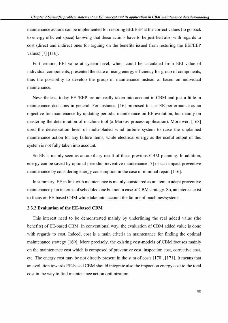
Chapter 2 Scientific problem statement on EE concept and its application in CBM maintenance decision-making
40
maintenance actions can be implemented for restoring EEI/EEP at the correct values (to go back
to energy efficient space) knowing that these actions have to be justified also with regards to
cost (direct and indirect ones for arguing on the benefits issued from restoring the EEI/EEP
values) [7] [116].
Furthermore, EEI value at system level, which could be calculated from EEI value of
individual components, presented the state of using energy efficiency for group of components,
thus the possibility to develop the group of maintenance instead of based on individual
maintenance.
Nevertheless, today EEI/EEP are not really taken into account in CBM and just a little in
maintenance decisions in general. For instance, [16] proposed to use EE performance as an
objective for maintenance by updating periodic maintenance on EE evolution, but mainly on
mastering the deterioration of machine tool (a Markov process application). Moreover, [168]
used the deterioration level of multi-bladed wind turbine system to raise the unplanned
maintenance action for any failure items, while electrical energy as the useful output of this
system is not fully taken into account.
So EE is mainly seen as an auxiliary result of these previous CBM planning. In addition,
energy can be saved by optimal periodic preventive maintenance [7] or can impact preventive
maintenance by considering energy consumption in the case of minimal repair [116].
In summary, EE in link with maintenance is mainly considered as an item to adapt preventive
maintenance plan in terms of scheduled one but not in case of CBM strategy. So, an interest exist
to focus on EE-based CBM while take into account the failure of machines/systems.
2.3.2 Evaluation of the EE-based CBM
This interest need to be demonstrated mainly by underlining the real added value (the
benefits) of EE-based CBM. In conventional way, the evaluation of CBM added value is done
with regards to cost. Indeed, cost is a main criteria in maintenance for finding the optimal
maintenance strategy [169]. More precisely, the existing cost-models of CBM focuses mainly
on the maintenance cost which is composed of preventive cost, inspection cost, corrective cost,
etc. The energy cost may be not directly present in the sum of costs [170], [171]. It means that
an evolution towards EE-based CBM should integrate also the impact on energy cost to the total
cost in the way to find maintenance action optimization.

Chapter 2 Scientific problem statement on EE concept and its application in CBM maintenance decision-making
41
This energy cost can be related for a major part by implementing the “required monitoring”
of the EEI/EEP. The monitoring can be done by sensors (direct monitoring) or by inspections
knowing that implementing a monitoring system can reduce the cost and frequency of inspection
task but increases the capital investment of the manufacturing system [95], [172]. For example,
Jin [173] used power consumption to map all potential failure modes with railway point
machines without deploying directly inspection task. So, an energy monitoring system can be
used to locate faults in manufacturing system [23] which can help to reducze the inspection time
and related costs (e.g. production loss when implementing inspection task).
In summary, this EE consideration in CBM in terms of “condition” but also in terms of the
benefits to be supported (with a specific focus on cost by integrating inspection cost, sensor cost
etc.) leads to isolate a fourth scientific issue which is:
Foundation of EE-based CBM [Scientific issue n°4]
2.4 Conclusions
The chapter 2 focused, from the two challenges identified in chapter 1, on the scientific
problem statement related to them. It leads to defend EEI as an emergent sustainability indicator
and as relevant KPI for maintenance decision-making in manufacturing system. EEI is then
considered through its evolution in the dynamic context of the system to argue the EEP concept.
These static and dynamic considerations of EE allows to conclude on the pertinence of EEI/EEP
on several abstraction levels (component, function, system level) of manufacturing system in the
way to aid decision-making. Finally, investigation of integrating EEI/EEP into CBM strategies
is studied.
Therefore, from the problem statement developed, we have positioned 4 main scientific issues:
- Definition and formalization of Energy Efficiency Indicator - EEI usable in decision-
making process of industrial (manufacturing) system (Scientific issue n°1);
- Foundation of an energy efficiency performance (EEP) concept for evaluating
residual life energy (Scientific issue n°2);
- Development of generic approach for prognostics of EEI at different levels of a
manufacturing system (Scientific issue n°3);
- Foundation of EE-based CBM (Scientific issue n°4).

Chapter 2 Scientific problem statement on EE concept and its application in CBM maintenance decision-making
42
These scientific issues are the basis to found our contributions developed then on the next
chapters as follows:
Chapter 3 tackles the scientific issue n°1 and n°2, by detailing the EEI/EEP concept and
develop a generic formalization of EEI/EEP at each level of abstraction (component, function,
system) of an industrial system.
Chapter 4 addresses scientific issue n°3 by proposing a generic approach for prognostics of
the evolution of EEI allowing to estimate the time left before the manufacturing system loses its
energy efficiency property.
Chapter 5 aims at validating the contributions developed in chapter 3 and 4. In that way, the
contributions are applied on TELMA platform.
Chapter 6 tackles scientific issue n°4 by contributing with the foundation of integrating EE
into CBM decision-making. This contribution is also illustrated in TELMA platform.

Chapter 3 EEI and REEL: concept and formulation for industrial applications
43
Chapter 3 EEI and REEL: concept and formulation for industrial applications
3.1. Introduction
This chapter describes the contributions we proposed with regards to the two first scientific
issues identified in chapter 2. In fact, we present an EEI concept with consideration of time-
dependent degradation behavior for manufacturing systems at several abstraction levels such as
component, function/system levels. In addition, the quantification of EEI by means of EEI
formulations is proposed to evaluate its values. Since EEI may deteriorate with time, a question
arising is when EEI reaches its critical threshold which could be seen as an energy efficiency
property/target to be guaranteed. In that way, we propose a novel concept, namely the Remaining
Energy-Efficient Lifetime (REEL), for representing energy efficiency performance (EEP) in an
anticipation vision. REEL can be used for various decisions-making processes but mainly in
maintenance ones (e.g. maintenance optimization) to be consistent with the frame of this thesis.
3.2. Concepts of energy efficiency indicators for industrial systems
As already defended in chapter 1, in manufacturing systems, both energy consumption and
useful output [47], [57], [81] are two main information to be mastered by owner. The
characteristics of this information allow to form the different categories of EEI normally usable
at the different abstraction levels of the decision-makers mainly in terms of energy consumers
and usage functions. Nevertheless, any of these categories can be used directly to fix these EEI
requirements as shown in Table 4 of chapter 1 and leading to a first part of the scientific issue
n°1 which is related to EEI identification. In that way, we propose a more general classification
of these EEIs based on their potential applications (Figure 8).
Chapter 3 EEI and REEL: concept and formulation for industrial applications
44
Figure 8. Concepts of EEI and their potential applications [174]
This classification highlights that the different EEI concerned by manufacturing levels are
located from “global system” to “components/equipment” (level aggregation axis). Moreover,
only the category related to “physical-thermodynamic indicators” (see chapter 2) is highlighted
to serve as a basis for formulating these EEI on these levels. Indeed, physical-thermodynamic
indicators integrate items as energy consumption and products delivery. Thus, based on the
category of physical-thermodynamic indicators, and to answer to the formulation need express
in scientific issue n°1, we propose, for manufacturing, to define EEI as:
𝐸𝐸𝐼 =E
O, (3.1)
where E is the total used energy input, 𝑂 is the useful output in physical units.
By definition, EEI provides the amount of energy consumed to produce a useful output unit.
So, the lower the EEI value is, the lower consumed energy to produce one unit of useful output.
EEI could be used in various decision-making processes, e.g., maintenance, control decision-
making. For example, based on the current value of EEI of a component, efficiency of the
component in using energy can be evaluated, and then decision-makers can choose whether to
trigger a preventive maintenance action on components or not.
In link to the decision-making needs, the previous formulation has to be investigated on
different abstract levels. In the frame of thesis, we focus only on two layers: component level
and function/system one.
Chapter 3 EEI and REEL: concept and formulation for industrial applications
45
3.2.1 Energy efficiency indicator at component level
The “component” is seen as the basic element which works with others at downstream level
to perform the function of upstream level. By using Equation (3.1), EEI of a component i at time
t is defined as follows:
𝐸𝐸𝐼𝑖(𝑡) =𝐸𝑖(𝑡)
𝑂𝑖(𝑡), (3.2)
where 𝐸𝑖(𝑡), 𝑂𝑖(𝑡) are respectively the energy consumed and the useful output of component
i within one time unit (from (t-1) to t). The time unit could be an hour, a day, a month, etc.
depending on the time interval of decision-making. We assume that the output of component i
is unique and measurable. It should be noted that when the output of a component is uncountable
or invisible such as when an electrical equipment or production process unit is pending and its
auxiliary system may however remain running and consuming energy, the definition of EEI is
slightly different. In fact, in this case, EEI is the ratio of energy inputs to energy outputs [175].
In that way, 𝑂𝑖(𝑡) in Equation (3.1) represents the energy useful output ( hidden in physical
outputs) and EEI mean (consist with the thermodynamic indicator).
In fact, component i may consume different kinds of energy sources which comes in different
common forms (gas, fossilized fuels, electricity, light, etc.) and measured by International
System (SI) of Units (Btu or BTU (British Thermal Unit), ton of coal equivalent (tce), kilowatt-
hours (kWh), Joules (J), etc.). Thus, to calculate the total energy of a component, its energy
inputs expressed in different forms need to be converted into a common unit. Then, the total
energy consumption of component i, which uses different energy sources (measured by tons of
coal, kWh, etc.), can be calculated with following formulation:
Ei(t) = ∑ θijETij(t)
l
j=1
, (3.3)
where 𝐸𝑖(𝑡) is the total energy consumed by component i, 𝐸𝑇𝑖𝑗(𝑡) is the amount of consumed
energy sources j (j=1-l), 𝜃𝑖𝑗 is energy conversion factor of the energy type j to the common
energy unit of component i. The conversion factor 𝜃𝑖𝑗 between different energy units is based
on the SI units, e.g., 1 Wh = 3.412 Btu, 1 tons of coal = 19,882,000 Btu. The energy consumption
𝐸𝑇𝑖𝑗(𝑡) of energy type j (measured by Wh, Btu, etc.) can be monitored or calculated directly by
different power meters.

Chapter 3 EEI and REEL: concept and formulation for industrial applications
46
In the same manner, component i may produce different types of products/services. A
common product (the number/hours of services, tons of steel, etc.) needs to be defined to
measure the amount of useful output. The output conversion factor of each type of product is the
amount of common output which is considered equivalent to one unit. Actually, the output
conversion factor for each product is fixed in advance by the decision-maker. In that way, if
component i produces m types of product in one period, its total outputs measured/converted in
common unit of output can be calculated as:
𝑂𝑖(𝑡) = ∑ 𝛾𝑖𝑗𝑂𝑇𝑖𝑗(𝑡)
𝑚
𝑗=1
, (3.4)
where 𝛾𝑗𝑖 is the conversion factor of the output type j in the common unit of output of
component i, and 𝑂𝑇𝑖𝑗(𝑡) is the amount of product type j (j=1-m).
Example 3.1:
Consider a system which is composed of 3 machines M1, M2 and M3. The structure of the
system is shown in Figure 9. The physical output of the system, namely product B, is processed
through two phases: phase 1 on machine M1 and phase 2 on machines M2 or M3. The
intermediate products A, which is the physical output of machine M1, are needed to produce the
final product B of system. 60% output of M1 enters M2 and the rest enters M3. It is assumed
that, at time t, the energy consumption of M1, M2 and M3 is 20kWh, 3412 Btu and 30 kWh
respectively. The useful outputs of M1, M2, and M3 are 200, 40 and 60 products per hour
respectively.
Figure 9. Manufacturing system of 3 components
M1
M2
M3
𝐸1(t) = 20 𝑘𝑊ℎ
𝐸2(t) = 3412 𝐵𝑡𝑢
𝐸3(t) = 30 𝑘𝑊ℎ
𝑂1 = 200 𝑂3 = 60
𝑂2 = 40
A
B
B
40%
60%
Chapter 3 EEI and REEL: concept and formulation for industrial applications
47
By using Equation (3.2), we obtain EEIs at the component level. Hence, EEIs for M1, M2
and M3 are EEI1(t) =20
200= 0.1 (kWh per product ), EEI2(t) =
3412
40= 85.3 (Btu per
product), and EEI3(t) =30
60= 0.5 (kWh per product) respectively.
3.2.2 Energy efficiency indicator at the function/system level
We focus now on a function or system which is composed of n components interconnected
according to a given configuration. It is assumed that only one kind of useful outputs of the
function/system is considered. We are interested in the evaluation of EEI for this function/system
from the EEI values at component level by bottom-up methods.
Based on Equation (3.2), EEI for this function/system is expressed as follows:
𝐸𝐸𝐼𝛴(𝑡) =𝐸𝛴(𝑡)
𝑂𝛴(𝑡), (3.5)
where 𝐸𝛴(𝑡), 𝑂𝛴(𝑡) are the total energy consumption and the total useful outputs during one
time unit (from (t-1) to t).
In one hand, we assume here a unique unit of Ei for each component i. The unique unit of
energy input for different components may also be different. To evaluate the total consumed
energy of the function/system, all energy input of downstream components need to be converted
to a common one, e.g. kWh. Moreover, 𝐸𝛴(𝑡) may not equal the sum of the total input energy
of each component [57] due to the energy transformation from upstream components to
downstream ones according to the energy flows direction. Nevertheless, the total input energy
of a function/system can be calculated from the input energy of its components. In that way, we
propose the following evaluation equation:
𝐸𝛴(𝑡) = ∑ 𝜆𝑖𝐸𝑖(𝑡)
𝑛
𝑖=1
, (3.6)
where λi represents the energy weighting factor. An energy weighting factor of any
component link directly to its consumed energy and energy-losses (cannot be transferred to other
components), which mainly depend on the dynamic context of the manufacturing system
(formulated as impact factors in EEI formalization). As an illustration, for the manufacturing
system above (Example 3.1), all components directly consume the imported energy and unique
unit of the total consumed energy is kWh, thus λ1 = λ3 = 1 and λ2 = 0.000293. As a result,
the total consumed energy is EΣ(t) = E1(t) + 0.000293 ∗ E2(t) + E3(t) = 60 (kWh).

Chapter 3 EEI and REEL: concept and formulation for industrial applications
48
On the other hand, the output may have different types of products/services. The converting
task to add multiple forms of outputs should be considered. In this case, it is needed to consider
the weighting factor of separate systems or unit processes to produce one output type as:
𝑂𝛴(𝑡) = ∑ 𝜇𝑖𝑂𝑖(𝑡)𝑛𝑖=1 , (3.7)
where μi stands for the output weighting factor associated to component i. In case of the
common form of physical output volume is fixed at this upstream level, the output weighting
factor μi can be used to express the change in the real physical output of each component at
downstream level, and the variation in the prices effects has been ignored to avoid the impact of
having different units [131], [176]. The weighting factors for different products present
appropriately the amount of energy needed to produce each of the products [176] and remaining
constant for all time points in the analysis.
Although Equation (3.5) can be used to calculate EEIs at upstream levels, but it can
demonstrate the relationship between the EEIs of upstream levels and downstream levels of
industrial system. By replacing the measured/stochastic values of total energy consumption and
total physical output presented, with calculated values by Equations (3.6), (3.7) into Equation
(3.5), EEI for a function/system is defined as:
𝐸𝐸𝐼𝛴(𝑡) =∑ 𝜆𝑖𝐸𝑖(𝑡)𝑛
𝑖=1
𝑂𝛴(𝑡)= ∑ 𝜆𝑖
𝑛
𝑖=1
𝑂𝑖(𝑡)
𝑂𝛴(𝑡)
𝐸𝑖(𝑡)
𝑂𝑖(𝑡) (3.8)
→ 𝐸𝐸𝐼𝛴(𝑡) = ∑ 𝜆𝑖𝑛𝑖=1 𝜔𝑖(𝑡)𝐸𝐸𝐼𝑖(𝑡) (3.9)
with 𝜔𝑖(𝑡) =𝑂𝑖(𝑡)
𝑂𝛴(𝑡) (3.10)
It is clear that Equation (3.9) allows evaluating EEI of a function/system from EEIs of its
components. These weighting factors may be not always available and need to be estimated.
Furthermore, they are may be time-dependent. It should be noticed that several approaches have
been proposed to support the weighting factors consideration for energy efficiency applications
(energy consumption and output) at multi-levels of industrial sectors [27], [131]. For example,
several approaches can be used to calculate these weighting factors [27], [53], [176]–[178].
Example 3.2:
Reconsider the example 3.1 presented in Figure 9, the total output of the system is 𝑂Σ = 𝑂2 +
𝑂3 = 100 products per hour (𝜇1 = 0, 𝜇2 = 𝜇3 = 1). EEI for the system can be calculated in
Chapter 3 EEI and REEL: concept and formulation for industrial applications
49
two ways. By using directly its definition presented by Equation (3.5), we get 𝐸𝐸𝐼Σ =𝐸Σ
𝑂Σ =
0.6 kWh per product. We can also obtain 𝐸𝐸𝐼Σ using the aggregation model presented by
Equation (3.9): 𝐸𝐸𝐼Σ(𝑡) = ∑ 𝜆𝑖𝑛𝑖=1 𝜔𝑖(𝑡)𝐸𝐸𝐼𝑖(𝑡) = 1 ∗ 2 ∗ 𝐸𝐸𝐼1 + 0.000293 ∗ 0.4 ∗ 𝐸𝐸𝐼2 +
1 ∗ 0.6 ∗ 𝐸𝐸𝐼3 = 0.6 (kWh
product) with 𝜔1 =
𝑂1
𝑂2+𝑂3 =200
100= 2; 𝜔2 =
𝑂2
𝑂2+𝑂3 =40
100= 0.4; 𝜔3 =
𝑂3
𝑂2+𝑂3 =60
100= 0.6 and 𝜆1 = 1; 𝜆2 = 0.000293; 𝜆3 = 1.
So these two Equation (3.5) and (3.9) are presented to calculate the EEI at upstream levels to
tackle the scientific issue n°1 about the formalization of EEI at system level (with EE data of
components). Indeed to calculate the EEI in the link from the downstream levels to the upstream
levels, the mathematic Equation (3.5) can be used to directly calculate the EEI at upstream level
when the measure of energy and physical output is available. By the same principle to convert
the different forms of energy and physical units, the weighting factors of each component at
downstream levels need to be calculated to estimate the final EEI at upstream level (Equation
(3.9)). EEI may be subjected to degradation with time due to the evolution of the manufacturing
system and its environment.
3.3. Remaining Energy-Efficient Lifetime
As presented in the chapter 2, mastering the EEI during the lifetime of industrial system
(knowing its evolution) can provide useful information for decision-maker during the decision-
making process. It means to consider EEI not only as a value but also its evolution as advocated
by EEP concept.
3.3.1 Concept of the Remaining Energy-Efficient Lifetime
It has been shown in a large number of works such as [52], [63], [158] that the energy
consumption and/or the useful output of an object (component, function or system) are usually
subject to degradation with time due to aging phenomena and/or the evolution of the operating
conditions. As a consequence, EEI may deteriorate with time. In relation to this degradation, we
can define a critical threshold, denoted 𝐸𝐸𝐼𝑇ℎ𝑟𝑒𝑠𝑜𝑙𝑑, by which an manufacturing object
(component, function/system) is considered as having lost its energy efficiency property when
its EEI value reaches the critical threshold. In that way, from a practical point of view, it is
interesting to know when the object loses its energy efficiency property as highlighted in chapter
2 (see section 2.2.3). This specific period of time (between current time and expected time when
the manufacturing system starts using energy inefficiently) leads to estimate the residual energy
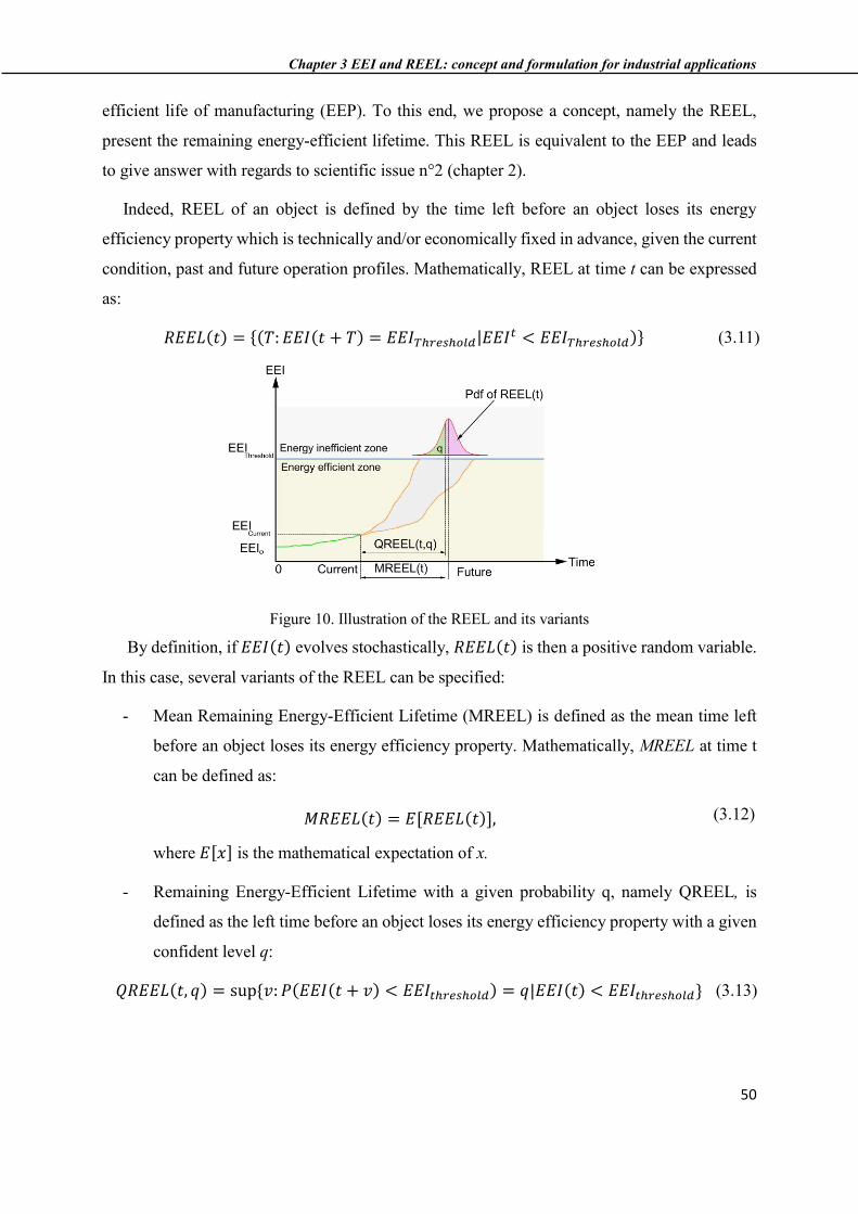
Chapter 3 EEI and REEL: concept and formulation for industrial applications
50
efficient life of manufacturing (EEP). To this end, we propose a concept, namely the REEL,
present the remaining energy-efficient lifetime. This REEL is equivalent to the EEP and leads
to give answer with regards to scientific issue n°2 (chapter 2).
Indeed, REEL of an object is defined by the time left before an object loses its energy
efficiency property which is technically and/or economically fixed in advance, given the current
condition, past and future operation profiles. Mathematically, REEL at time t can be expressed
as:
𝑅𝐸𝐸𝐿(𝑡) = {(𝑇: 𝐸𝐸𝐼(𝑡 + 𝑇) = 𝐸𝐸𝐼𝑇ℎ𝑟𝑒𝑠ℎ𝑜𝑙𝑑|𝐸𝐸𝐼𝑡 < 𝐸𝐸𝐼𝑇ℎ𝑟𝑒𝑠ℎ𝑜𝑙𝑑)} (3.11)
Figure 10. Illustration of the REEL and its variants
By definition, if 𝐸𝐸𝐼(𝑡) evolves stochastically, 𝑅𝐸𝐸𝐿(𝑡) is then a positive random variable.
In this case, several variants of the REEL can be specified:
- Mean Remaining Energy-Efficient Lifetime (MREEL) is defined as the mean time left
before an object loses its energy efficiency property. Mathematically, MREEL at time t
can be defined as:
𝑀𝑅𝐸𝐸𝐿(𝑡) = 𝐸[𝑅𝐸𝐸𝐿(𝑡)], (3.12)
where 𝐸[𝑥] is the mathematical expectation of x.
- Remaining Energy-Efficient Lifetime with a given probability q, namely QREEL, is
defined as the left time before an object loses its energy efficiency property with a given
confident level q:
𝑄𝑅𝐸𝐸𝐿(𝑡, 𝑞) = sup {𝑣: 𝑃(𝐸𝐸𝐼(𝑡 + 𝑣) < 𝐸𝐸𝐼𝑡ℎ𝑟𝑒𝑠ℎ𝑜𝑙𝑑) = 𝑞|𝐸𝐸𝐼(𝑡) < 𝐸𝐸𝐼𝑡ℎ𝑟𝑒𝑠ℎ𝑜𝑙𝑑} (3.13)
Chapter 3 EEI and REEL: concept and formulation for industrial applications
51
It is clear that MREEL and QREEL are deterministic. As a consequence, their uses for
decision-making could be simpler than REEL. Figure 10 illustrates the concept of the REEL and
its variants.
3.3.2 Evaluation of the Remaining Energy-Efficient Lifetime at component level
By definition, to evaluate the REEL of a component, it is necessary to quantify the potential
evolution of EEI. The energy consumption and/or the useful output may depend on different
impact factors. As a consequence, it is important to identify several impact factors/features that
impact the energy consumption and/or the useful output of a component. In a general manner,
we classify these impact factors into two categories: static factors (SF) which are impact factors
whose evolution in time is deterministic and often known in advance (e.g., production
planning/load profiles, human skills, etc.); dynamic factors (DF) whose evolution in time is
random and often unknown, e.g., environment condition, deterioration features, etc. To predict
the evolution of the DF, several existing prognostic approaches (see chapter 4.2) may be used.
Based on the value of these impact factors, the energy consumption E𝑖(t) and the useful
output O𝑖(t) may be directly evaluated. However, if the relationships between the impact factors
and the energy consumption/useful output may be stochastic and unknown, an estimation is then
needed.
In that way, a generic model of energy efficiency based on the proposed formulation of energy
consumption E𝑖(t) and useful output O𝑖(t) are the following:
𝐸𝐸𝐼𝑖(𝑡) =𝑓(𝑡, 𝑆𝐹𝐸 , 𝐷𝐹𝐸)
𝑔(𝑡, 𝑆𝐹𝑂 , 𝐷𝐹𝑂) (3.14)
𝐸𝑖(𝑡) = 𝑓(𝑡, 𝑆𝐹𝐸 , 𝐷𝐹𝐸) (3.15)
𝑂𝑖(𝑡) = 𝑔(𝑡, 𝐷𝐹𝑂 , 𝐷𝐹𝑂) (3.16)

Chapter 3 EEI and REEL: concept and formulation for industrial applications
52
Figure 11. The REEL evalution at the component level
It is important to note that f and g may be nonlinear or stochastic. Based on the future
evolution of EEI, the REEL can be evaluated. The illustration of the REEL evaluation process
is given by Figure 11.
Example 3.3:
We are considering another example related to water supply systems, for the consideration of
its EEI as a function of different impact factors. In relation to this system, [140] proposed the
equation to calculate the energy consumption:
𝐶𝐸𝐿 =𝜌. 𝑔. 𝑄. 𝐻
𝜂𝐵 . 𝜂𝑀. ∆𝑡 =
𝜌. 𝑔. 𝑄. (𝐻𝐺 + Σ𝑓.𝐿.𝑣2
𝐷.2.𝑔+ Σ
𝑘.𝑣2
2.𝑔)
𝜂𝐵 . 𝜂𝑀. ∆𝑡 (3.17)
Where:
𝐶𝐸𝐿 is the energy consumption by each motor-pump set [Wh];
𝜌 is the water density [kg/m3];
𝑔 is gravity acceleration [m/s2];
𝑄 is the pumped flow [m3/s];
𝐻 is the total height of the pump lift [m];
𝜂𝐵 and 𝜂𝑀 are pump and motor performance respectively [%];
∆𝑡 is the running time of the motor-pump set [hours];
𝐻𝐺 is the geometric head of the elevation [m];

Chapter 3 EEI and REEL: concept and formulation for industrial applications
53
𝑓 is the pipe friction factor [0-1];
𝐿 is the pipeline length [m];
𝑣 is the average flow velocity in the pipe [m/s1];
𝐷 is pipe diameter [m];
𝑘 is the coefficient of head loss of each singularity [0-1].
If the useful output is considered as the total volume of delivered water, the total output can
be calculated as:
𝑂𝐸𝐿 = 𝑄. ∆𝑡 (𝑚3) (3.18)
𝐸𝐸𝐼𝐸𝐿 =𝜌. 𝑔. (𝐻𝐺 + Σ
𝑓.𝐿.𝑣2
𝐷.2.𝑔+ Σ
𝑘.𝑣2
2.𝑔)
𝜂𝐵. 𝜂𝑀 (𝑊ℎ/𝑚3) (3.19)
In link to our frame, the two impact factors (geometric head (𝐻𝐺) and length of pipelines (𝐿))
are considered as static factors. Their values can be changed during the time but are known in
advance based on load development plan. The other impact factors (pump (𝜂𝐵) and motor (𝜂𝑀)
efficiencies, pipe friction factor (𝑓), quantity and condition of singularities (Σk)) are considered
as dynamic factors. By using the Equation (3.19) with the predicted value of its impact factors,
the EEI value of pumping can be predicted.
It is important to note that predicting the evolution of EEIs is a difficult task and cannot be
based on only one prognostics approach. For example, the deterioration of bearing, which
impacts the energy efficiency performance of rotating machines, may be predicted based on
vibration signals by using data-driven prognostic approaches [107], [179].
3.3.3 Evaluation of the Remaining Energy-Efficient Lifetime at higher level
At the function/system level, the operation programs or system functions have strong impacts
on the running modes of each component. An efficient equipment could lose its optimal working
point with regard to the running modes of the system. In this case, there is a high opportunity in
energy efficiency improvement at system level due to the non-optimal working points, lack of
skills of operators or low awareness of managers [60].
Firstly, the energy consumption and the useful output of lower level units can be changed
according to various system structures, which are defined as set of operation procedure of lower
level units i.e. components. Indeed, several operation profiles can be implemented to conduct

Chapter 3 EEI and REEL: concept and formulation for industrial applications
54
functions of an industrial system. Thus the contribution of each lower level unit to the energy
consumption and the useful output of higher levels may be modified thereby. For example, in
the hot-dip galvanized steel sheet production process, if the thickness of steel sheet output is
decreased, the motor-driven roller system will consume more electrical energy while the energy
consumption of the auxiliary systems like lighting and conveyors is seen unchanged. The system
boundaries, constraints and future operation profiles that can impact EEI have to be identified
and classified [180].
Instead of only using the predicted energy consumption and the useful output of lower level
components, the contribution of all components is requested to calculate EEIs at the
function/system level. The contributions of components are influenced by future operation plans
which can be a set of operation modes corresponding to any forecasted production requirements.
From Equation (3.9), EEIΣ(𝑡) for a function/system at any time point t is affected by the
weighting energy factors, the weighting physical factors of all components and other parameters
such as system structures, dependencies between components, production schedules, support
systems, operation conditions and management. Information on the function or system will be
used to assess the weighting factors associated with overall energy consumption and those
related to productivity. It is necessary to note that these factors may change over time. Figure 12
illustrates the process of predicting REEL at the level of a function or a system.
Figure 12. Procedure to evaluate REEL at function/system level
At this stage now, it is necessary to predict the potential evolution of EEIs in order to estimate
the REEL. It is however noticed EEIs may depend on different factors (SF and DF), hence
predicting the potential evolution of EEIs may be not easy.

Chapter 3 EEI and REEL: concept and formulation for industrial applications
55
3.4. Conclusion
In this chapter, with regards to the first scientific issue, an energy efficiency indicator (EEI)
based on the physical-thermodynamic indicators analysis is defined at both component and
function/system level of a manufacturing system. This EEI concept is developed to be consistent
with existing EE standards/frameworks. It can be expressed as the ratio of energy input over the
useful output of industrial system and this for different abstraction levels. Then a general
formulation of EEI is proposed by taking into account the static and dynamic impact factors by
using Equations (3.14), (3.15), and (3.16). In order to evaluate the EE performance to tackle the
second scientific issue, a novel concept namely remaining energy-efficient lifetime (REEL)
providing the time left before a component/function/system losses its energy efficiency property
is proposed. This concept can be seen as a transformation of RUL concept and the generic
formalization of REEL is constructed on the Equations (3.11), (3.12) and (3.13). In that way,
REEL is representative of EEP in the future. Based on the developed concept and formulation
of EEI/REEL, in the next chapter a generic approach will be developed to predict the potential
evolution of EEI and estimate REEL.
Furthermore, the use of EEI/REEL in condition-based maintenance decision-making will be
described in Chapter 6.

Chapter 3 EEI and REEL: concept and formulation for industrial applications
56
Chapter 4 Generic approach for prognostics of the evolution of EEI and REEL
57
Chapter 4 Generic approach for prognostics of the evolution of EEI and REEL
4.1. Introduction
This chapter describes our contribution related to the scientific issue n°3 pointed out in
chapter 2. As mentioned in chapters 1 and 2, predicting the evolution of EEI is crucial for
estimating REEL. It is however shown that the existing prognostic approaches cannot be directly
used to support this prediction due to the complexity of EEI. Therefore we propose, in this
chapter, a generic approach which can help to select the appropriate existing prognostic
approaches and their combination for predicting the potential evolution of EEI and estimating
REEL. In that way, a short review on the existing prognostic approaches are firstly discussed.
This provides a classification on the prognostic models and their potential applications. A
generic approach for prognostics of EEI/REEL, from theses existing prognostics models, at both
component and function/function level is then proposed. This approach is based on the three
steps and each step is detailed.
4.2. Short review on existing prognostic approaches for RUL prediction
Indeed, predicting the EEI evolution in link to the dynamic context of the system (e.g. impact
factors) could be referred to the use of conventional prognostic approaches to predict the RUL
of component/system. For the prediction of the RUL, a large number of prognostic approaches
have been proposed and classified into three categories (Figure 13):
Experience-Based Prognostics: This type of approach is based on the exploitation of
knowledge on the failure or degradation of systems for the prediction of the RUL.
Experience-based prognostic approaches are quite simple and less expensive to be
implemented [181], [182]. However, these approaches are hardly applicable in a
dynamic environment where a system and/or its environment evolve dynamically
over time. Indeed, experience-based prognostic approaches strongly depend on the
competence of experts and engineering. In addition, prognostic results are less
accurate than model-based and data-driven prognostic methods. Nevertheless, this
kind of approaches could be useful when historical data is very limited.

Chapter 4 Generic approach for prognostics of the evolution of EEI and REEL
58
Model-Based Prognostics: These approaches are mainly based on
analytical/mathematical models to describe behaviors of systems and mechanisms of
degradation phenomenon [183], [184]. Main advantages of model-based approaches
are their high accuracy and flexibility in configuring input data. Of course, prediction
accuracy of these approaches depends on the precision of the presented models.
Furthermore, nonlinear and stochastic characteristics of industrial systems may
increase the difficulty in building analytical models. The flexible configuration of
systems impact the model parameters. Thus, these situations have to be taken into
account in the real-time modifications of these models.
Data-driven Prognostics: These approaches allow to identify trends/patents of a
developing fault and to predict the amount of time before it reaches a predetermined
threshold [185]–[187] using information from historical treated data (trained data).
These prognostic approaches can identify the real-time health condition of a system
by various techniques such as regression analyses, Bayesian algorithms, neutral
networks, fuzzy logics, support vector machine… These prognostic approaches are
more precise than the first type of approaches (experience-based prognostics), in their
ability to link with recognized system behaviors by experience methods. Despite no
specific physical model is needed, the data-driven approaches require a monitoring
system and learning time.
Figure 13. Classification of prognostic approaches [188]
Depending on the type of prognostics approaches, various types of information are required
such as engineering models and data, failure history, past operating conditions, current

Chapter 4 Generic approach for prognostics of the evolution of EEI and REEL
59
conditions, identified fault patterns, maintenance history and system degradation. Otherwise,
RUL is mostly considered just for only one or scale “condition”, which is usually presented by
only one degradation indicator.
As recently mentioned in several studies, the hybrid-prognostics are mentioned to leverage
the advantages of different prognostics models [165], [189]. The basic principal of this work are
combines two or three previous approaches in a close loop to get benefits and limit their
drawbacks. More reliable and accurate prognostics results obtained by hybrid approach are
claimed [190].
4.3. Global view of the proposed generic approach for prognostics of the EEI evolution and
REEL
So, in link to the conventional prognostics approaches previously presented, we propose a
generic approach for predicting the evolution of EEIs, which is structured on three main steps
(Figure 14):
Figure 14. Generic approach for prognostic of the evolution of EEI
Step 1 – Energy efficiency modeling: The objective of this step is to formulate the energy
consumption and the useful output. In this sense, first, several impact factors (degradation
physical health, material quality, etc.) have to be identified and, then, the relationship between
the impact factors and both the energy consumption and the useful output should be formulated.
These impact factors already have been taken into account to develop the Equations (3.14),
(3.15), and (3.16) of chapter 3.
Step 2 - Prediction of the potential evolution of impact factors: The objective of this step is
to forecast the evolution of impact factors identified in Step 1 according to the future operation
profiles. By using an appropriate prognostic model, the future evolution of these impact factors
may be tracked.
Step 3 – Evaluating the evolution of EEIs and estimating the REEL: The aim of this step is to
predict the evolution of EEIs, thereby estimating the REEL defined in Equation (3.11) by taking
into account the results given in Step 2.

Chapter 4 Generic approach for prognostics of the evolution of EEI and REEL
60
The procedure for applying a generic approach for prognostics of the evolution of EEIs is
illustrated in Figure 15. This procedure can be developed both at the component level and at
function/system levels. It is important to note that the process for components (the left part of
Figure 15) is linked to the procedure for the function/system level (the right part of Figure 15).
The following detailed procedures concretize and detail the generic approach leading to the
scientific issue n°3 which is related to EEI prediction at different levels of manufacturing system.
Figure 15. Generic approach for prognostic of the EEI evolution to estimate the REEL
4.4. Step 1: Energy efficiency modeling
As discussed in chapter 3 (section 3.2), it is necessary for modeling the energy efficiency (the
energy consumption and the useful output) to calculate EEIs at different time points. The
formulation of taking into account identified impact factors is the main achievements of this
step.
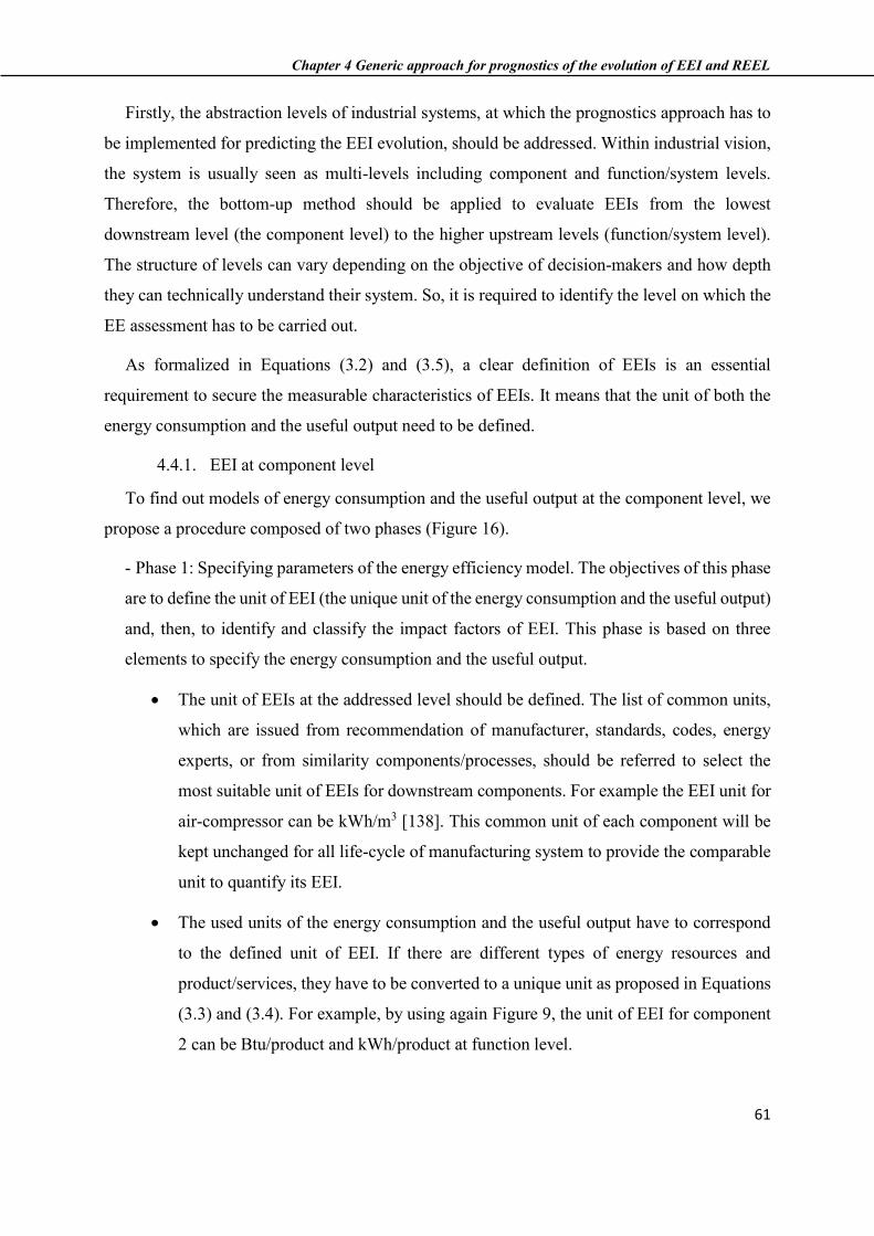
Chapter 4 Generic approach for prognostics of the evolution of EEI and REEL
61
Firstly, the abstraction levels of industrial systems, at which the prognostics approach has to
be implemented for predicting the EEI evolution, should be addressed. Within industrial vision,
the system is usually seen as multi-levels including component and function/system levels.
Therefore, the bottom-up method should be applied to evaluate EEIs from the lowest
downstream level (the component level) to the higher upstream levels (function/system level).
The structure of levels can vary depending on the objective of decision-makers and how depth
they can technically understand their system. So, it is required to identify the level on which the
EE assessment has to be carried out.
As formalized in Equations (3.2) and (3.5), a clear definition of EEIs is an essential
requirement to secure the measurable characteristics of EEIs. It means that the unit of both the
energy consumption and the useful output need to be defined.
4.4.1. EEI at component level
To find out models of energy consumption and the useful output at the component level, we
propose a procedure composed of two phases (Figure 16).
- Phase 1: Specifying parameters of the energy efficiency model. The objectives of this phase
are to define the unit of EEI (the unique unit of the energy consumption and the useful output)
and, then, to identify and classify the impact factors of EEI. This phase is based on three
elements to specify the energy consumption and the useful output.
The unit of EEIs at the addressed level should be defined. The list of common units,
which are issued from recommendation of manufacturer, standards, codes, energy
experts, or from similarity components/processes, should be referred to select the
most suitable unit of EEIs for downstream components. For example the EEI unit for
air-compressor can be kWh/m3 [138]. This common unit of each component will be
kept unchanged for all life-cycle of manufacturing system to provide the comparable
unit to quantify its EEI.
The used units of the energy consumption and the useful output have to correspond
to the defined unit of EEI. If there are different types of energy resources and
product/services, they have to be converted to a unique unit as proposed in Equations
(3.3) and (3.4). For example, by using again Figure 9, the unit of EEI for component
2 can be Btu/product and kWh/product at function level.

Chapter 4 Generic approach for prognostics of the evolution of EEI and REEL
62
Figure 16. Diagram for modeling energy efficiency of manufacturing systems
All impact factors of the energy consumption and the useful output should be
identified and classified into SF and DF. This classification aims at defining what
impact factors should be applied to prognostic approaches for predicting their
evolution in the next step.
All available energy data is collected through the acquisition/monitoring system to provide
efficient relevant data at different layers of the application.
- Phase 2: Selection of the prognostics approach for EEI prediction. If an energy efficiency
model (energy consumption model and/or useful output model), which is a function of
identified impact factors, already exists, this model can be used as the final selected energy
efficiency model of the first step. Otherwise, models of the energy consumption and the useful
output need to be developed. The proposed procedure to select and/or to develop an
appropriate model for energy efficiency (process F1 for energy consumption modeling and
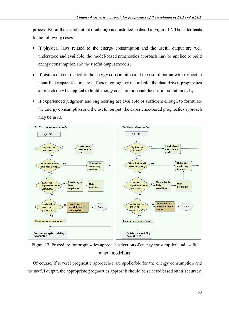
Chapter 4 Generic approach for prognostics of the evolution of EEI and REEL
63
process F2 for the useful output modeling) is illustrated in detail in Figure 17. The latter leads
to the following cases:
If physical laws related to the energy consumption and the useful output are well
understood and available, the model-based prognostics approach may be applied to build
energy consumption and the useful output models;
If historical data related to the energy consumption and the useful output with respect to
identified impact factors are sufficient enough or recordable, the data-driven prognostics
approach may be applied to build energy consumption and the useful output models;
If experienced judgment and engineering are available or sufficient enough to formulate
the energy consumption and the useful output, the experience-based prognostics approach
may be used.
Figure 17. Procedure for prognostics approach selection of energy consumption and useful
output modelling
Of course, if several prognostic approaches are applicable for the energy consumption and
the useful output, the appropriate prognostics approach should be selected based on its accuracy.

Chapter 4 Generic approach for prognostics of the evolution of EEI and REEL
64
In that way, the model-based prognostics should be the first priority in modeling (see section
4.2).
4.4.2. EEI at higher level
If a higher level has to be addressed, the definition of both input and output (energy and
physical output) are firstly prerequisite to determine common units of each component at
downstream levels and higher upstream level. Then, the main components contributing to the
energy consumption and the useful output at this level should be identified (knowing that the
energy efficiency modeling has previously been developed for each component). However, the
contribution of the components is influenced by future operation plans of functions/systems.
Thus the impact of function/system factors such as energy and work flows, management plans,
production plans need to be taken into account.
In order to technically understand the transformation of both energy and material between
components to produce the final manufactured product at higher level, an energy flows diagram
and production diagram need to be provided in advance (by external energy experts or
experience data). This allows to assess the hidden energy and resources in each unit of output,
then to identify which components at downstream level can have strong contribution on the EEI
at higher level (as well the areas that can have major change in the future). Indeed, the energy
flow diagram is a graph which illustrates the energy transfer between components and how
energy can be transformed and distributed between these components. Figure 18 illustrates the
energy flow in the case of a fan system which is combined from three main components (the
control system, the electrical motor and the centrifugal fan) [174], [191]. The figure shows the
relationships and the effects of an individual component on the others.
Figure 18. Energy flow and Air flow output of fan system
Motor Fan
Thermal
losses
Control system
Switching/Thermal
losses
Copper losses Core losses
Stray
losses
Aerodynamic
losses
Air flow Electrical
power input

Chapter 4 Generic approach for prognostics of the evolution of EEI and REEL
65
In that ways, energy and material flows are analyzed to realize the contribution of each
component to the energy consumption and the useful output at this level. This is important to
visualize how the input energy is distributed to downstream component. Then the impact of these
components will be materialized by their weighting factors (𝜆𝑖, 𝜔𝑖) as formulated in Equations
(3.6) and (3.7). Then, the aggregate formulation for calculating EEIs as proposed in Equation
(3.9) is used to estimate the energy efficiency performance at the function/system level. It is
important to note that going from energy and material flow diagrams to weighting factors
(𝜆𝑖, 𝜔𝑖) might be not so obvious.
At the end of Step 1, the energy efficiency model (with the formulation of the energy
consumption and the useful output) including the operation conditions (the impact factors and
operation profiles) need to be achieved. The evolution in the future of the identified and
classified impact factors will be predicted in Step 2. Then their evolution will be used with the
energy efficiency model for predicting the evolution of energy efficiency at Step 3.
4.5. Step 2: Prediction of the potential evolution of impact factors
The second step of the proposed generic approach is to forecast the evolution of impact factors
of the energy consumption and the useful output. This step is based on conventional prognostic
approaches. In order to do so, the future operation profile (FOP) must be identified.
4.5.1. At component level
The potential evolution of the impact factors (both SF and DF), which are already identified
and classified in Step 1, should be forecasted regarding to FOP. To support this task, a procedure
is proposed and illustrated in Figure 19.
Firstly, SF, whose evolution in time is deterministic, are usually easy to be observed in
advance. We just make a calculation of these SF at any time point in the future to forecast their
evolution.
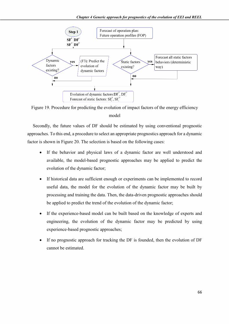
Chapter 4 Generic approach for prognostics of the evolution of EEI and REEL
66
Figure 19. Procedure for predicting the evolution of impact factors of the energy efficiency
model
Secondly, the future values of DF should be estimated by using conventional prognostic
approaches. To this end, a procedure to select an appropriate prognostics approach for a dynamic
factor is shown in Figure 20. The selection is based on the following cases:
If the behavior and physical laws of a dynamic factor are well understood and
available, the model-based prognostic approaches may be applied to predict the
evolution of the dynamic factor;
If historical data are sufficient enough or experiments can be implemented to record
useful data, the model for the evolution of the dynamic factor may be built by
processing and training the data. Then, the data-driven prognostic approaches should
be applied to predict the trend of the evolution of the dynamic factor;
If the experience-based model can be built based on the knowledge of experts and
engineering, the evolution of the dynamic factor may be predicted by using
experience-based prognostic approaches;
If no prognostic approach for tracking the DF is founded, then the evolution of DF
cannot be estimated.

Chapter 4 Generic approach for prognostics of the evolution of EEI and REEL
67
Figure 20. Procedure for selecting prognostic approaches to predict the evolution of a dynamic
factor
4.5.2. At higher level
At this addressed level, the FOP may condition the configuration and operation mode of the
components. In that way, the set of impact factors of all components has to be determined
according to the modification of mission profiles in the future.
At first, the FOP should be analyzed to identify its impact on the energy and material flows
within the addressed level. Then the contribution to the energy consumption and the useful
output of each component will be converted into its weighting factor corresponding to different
energy and material flows. At the end, a set of weighting factors of all components are collected
at any time point in the future.
It is essential at the end of Step 2 that the evolution of both dynamic and static factors needs
to be forecasted. Their evolution will be used by the energy efficiency model to evaluate the
evolution of energy efficiency in the next step under future mission profiles.

Chapter 4 Generic approach for prognostics of the evolution of EEI and REEL
68
4.6. Step 3: Evaluation of the evolution of EEI and estimation of REEL
The objectives of this step are to evaluate the potential evolution of EEIs and to estimate the
REEL regarding to a future condition. This step can be divided into two phases (Figure 21).
Figure 21. Procedure to evaluate the evolution of EEIs and to estimate the REEL
4.6.1. Phase 1: Evaluation of the evolution of EEI and estimation of REEL
The objective of this phase is to predict the EEI evolution which can help to estimate the
REEL at addressed levels. In this context, the achieved energy efficiency model of Step 1 (see
section 4.4) under the evolution of all impact factors is used to evaluate the future value of EEIs
at the addressed levels.
At the downstream level, the function of the energy consumption and the useful output
(results of Step 1) as the function of the predicted evolution of DF and the foreseen value of SF
(results of Step 2) are used to evaluate the EEI at any time in the future.
At the higher level, a set of weighting factors under the impact of the forecasted operation
profiles and EEI of each component at any time point in the future will be used to evaluate the
evolution of EEIs at the function/system level.
Chapter 4 Generic approach for prognostics of the evolution of EEI and REEL
69
The pre-set threshold and the specific context such as the probability q referred to section 0
should be used to estimate the REEL and its variants at both the component and function/system
levels, see again Equations (3.11), (3.12) and (3.13).
4.6.2. Phase 2: Online updating of the Remaining Energy-Efficient Lifetime
The aim of the phase 2 is to update the REEL if needed. This means that the estimated REEL
should be updated when new data/information on the current state is available. This can be done
by turning back to the second step for recalibrating the REEL.
By this step-by-step procedure, the EEI evolution can be predicted to estimate the REEL at
the addressed level (component/function/system levels). It is logical that the achieved REEL can
provide the useful information for aiding the maintenance decision-making.
4.7. Conclusion
In this chapter, the structure for predicting EEI evolution and the estimation of REEL lead to
support the scientific issue No.3, but the methods to implement these evaluations need to be
developed.
Through this approach, EEI assessment not only at past and current time but also its prediction
in the future is tackled thought a generic approach based on existing prognostic models. This
generic approach allows to predict the potential evolution of EEI at different level of
manufacturing system with a given mission profile using the formulation proposed in chapter 3.
Based on the EEI evolution, the REEL can be estimated regarding to the EEI critical threshold
which is associated with an energy efficiency property/performance. In fact, the proposed
generic approach is divided into three main steps and applicable at different abstraction levels
of a manufacturing system. These three steps are:
- Energy efficiency modeling (Step 1);
- Prediction of the potential evolution of impact factors (Step 2);
- Evaluating the evolution of EEIs and estimating the REEL (Step 3).
The proposed generic approach for prognostics of EEI/REEL is applied for a manufacturing
platform in the chapter 5.

Chapter 4 Generic approach for prognostics of the evolution of EEI and REEL
70

Chapter 5 Validation of the contributions in the case of TELMA platform
71
Chapter 5 Validation of the contributions in the case of TELMA platform
5.1. Introduction
To illustrate and validate the concepts introduced in chapter 3 and the proposed generic
approach for prognostics of EEI and REEL (chapter 4), a case study is investigated in this
chapter. Indeed, the investigation is brought to a manufacturing platform, called TELMA.
Firstly, at component level the impact factors (SF and DF) associated with each component are
identified. Since the analytical formulation of EEI is very difficult, some experimentations are
carried out to find numerically EEI which is a function of the impact factors. To predict the
potential evolution of EEI, the deterioration process of dynamic factors is simulated by a Gamma
deterioration process. The prediction result on EEI is then used to estimate the remaining energy-
efficient lifetime (REEL). For a higher level (function level), based on EEI at component level,
the EEI of the considered “punching” function is determined which can help to estimate the
REEL of this function.
5.2. Presentation of TELMA platform
TELMA platform is based on a real industrial application such as steel sheet cutting or metal
punching. TELMA is designed for conventional training activities, simulation of online
operation on industrial e-services and e-training in the e-Maintenance domains. TELMA
platform is based on 4 sub-systems: a bobbin changing, an advance motor-driven system (MD1),
an accumulator motor-driven system (MD2) and punching-cutting (Figure 22) [192]–[194].
Each sub-system consists of several components such as gear box, belt tensioner, motor, variable
speed drivers (VSDs) (Altivar with and remote I/O modules) and air-compressed valves. An
automated control system is fully dedicated to support the offline and online monitoring modes
by integrating a monitoring system (sensors, actuators, etc.), Human Machine Interface (HMI)
system (control screens, control boards, computers, Web-Cam, etc.), and programmable logic
controllers-PLCs (i.e. TSX premium with web interfaces). TELMA consumes mainly electrical
energy to form the “simulated” steel strip into shaped steel-sheets, and increasing the number of

Chapter 5 Validation of the contributions in the case of TELMA platform
72
formed steel-sheets (considered as the final output of TELMA) obtained per hour corresponding
to the main economic productivity performance of TELMA.
TELMA platform is also equipped with software and hardware components to be able to
simulate the degradation process (such as deterioration of bearing systems, belts and rollers) and
the failure modes like “Belt break”. Indeed, in TELMA platform, it is very difficult to create a
real deterioration phenomena or a real failure of the component due to the fact that (i) the
operating time of TELMA is not long enough for deterioration/failure appearing and (ii) failure
costs are very high (failed components costs). However, to develop experimentation related to
maintenance, several specific software and hardware are implemented on the platform (e.g. a
degradation software is on a PLC) to simulate the degradation behavior and failure on the system.
For example, the belt tensioner is used to simulate the failure event “Belt break” by releasing the
belt to the roller. The scenarios of degradation processes or failures are controlled by an
automated system (PLC connected to an online monitoring system).
Figure 22. Structure of the platform TELMA

Chapter 5 Validation of the contributions in the case of TELMA platform
73
5.2.1 Identification and classification of key components and the function/system
For the validation phase, we are focusing on the “punching” function of TELMA platform.
The “punching” function is realized by movement of the mechanical punch press, which is
driven by advance motor-driven system MD1, while accumulator motor-driven system MD2
continuously feeds the steel strip to holding position of pressor cylinder. About energy,
electricity is directly supply to two Altivar VSDs (provided by Schneider-electric Company) for
controlling the speed of two 3-phase induction motors (manufactured by LS Company). The
speed setting of these motor driven systems (MD1 and MD2) are related to rotation of the rollers
and the productivity of “punching” function of the TELMA.
As key components, we can identify in TELMA platform the followings:
A bobbin changing
An advance motor-driven system (MD1) with PLC controller
An accumulator motor-driven system (MD2) with PLC controller
Punching-cutting header
Air-compressor valve and piston
HMI control panel and online management system
In the frame of EE issue, we just consider the advance motor-driven system (MD1) and the
accumulator motor-driven system (MD2) as main energy consumers, the others key components
are not taken into account.
5.2.2 Description of the system and experimentation
With regards to this experimental context, we have taken the following assumptions for
TELMA.
Bearing is one of the most critical component of a motor-driven system knowing that its
working conditions (corrosion, lubrication, etc.) can strongly impact the “bearing frictional
losses”[195]. So, we consider here the deterioration of a motor-driven system as assimilated to
“bearing deterioration” given that the bearings implemented on TELMA is standard ball bearings
(manufactured by SKF with outside diameter D=35mm). Nevertheless, we cannot monitor the
real deterioration of bearing (no sensors, no direct inspection possible) but we can use brakes to
simulate “bearing deterioration”. Indeed, TELMA platform is equipped with electromagnetic
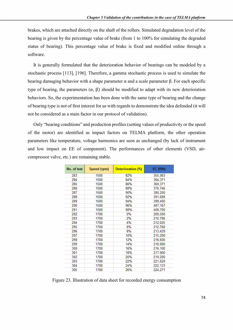
Chapter 5 Validation of the contributions in the case of TELMA platform
74
brakes, which are attached directly on the shaft of the rollers. Simulated degradation level of the
bearing is given by the percentage value of brake (from 1 to 100% for simulating the degraded
status of bearing). This percentage value of brake is fixed and modified online through a
software.
It is generally formulated that the deterioration behavior of bearings can be modeled by a
stochastic process [113], [196]. Therefore, a gamma stochastic process is used to simulate the
bearing damaging behavior with a shape parameter α and a scale parameter β. For each specific
type of bearing, the parameters (α, β) should be modified to adapt with its new deterioration
behaviors. So, the experimentation has been done with the same type of bearing and the change
of bearing type is not of first interest for us with regards to demonstrate the idea defended (it will
not be considered as a main factor in our protocol of validation).
Only “bearing conditions” and production profiles (setting values of productivity or the speed
of the motor) are identified as impact factors on TELMA platform, the other operation
parameters like temperature, voltage harmonics are seen as unchanged (by lack of instrument
and low impact on EE of component). The performances of other elements (VSD, air-
compressor valve, etc.) are remaining stable.
Figure 23. Illustration of data sheet for recorded energy consumption

Chapter 5 Validation of the contributions in the case of TELMA platform
75
5.3. Implementation of the generic approach for selection of EEI and related models:
architecture definition
On the basis of the assumptions selected, we applied the proposed generic approach for
prognostics of EEI and estimation of REEL, to component and function level of TELMA. In that
way, each three steps of the approach is detailed below with their application to TELMA.
5.3.1 Step 1: Energy efficiency modeling
As previously mentioned, only the “punching” function level of TELMA is addressed in this
study. To support the punching function, it is focusing on the energy efficiency of MD1 and
MD2 at the component level and the other auxiliary components are considered as non-
consuming energy parts (non-significant consumption). Hence, the scope of this case study is
limited to predict the evolution of EEI both at the component level and at the function level.
Then the REEL of the function level is estimated.
5.3.1.1 At component level:
It is important to note that, MD1 and MD2 are physically identical but functionally
independentl. Their speed is controlled by PLC to meet the productivity demand knowing that
this demand is materialized through the production plans, of which the productivity of punched
steel-sheets are known in advance.
5.3.1.1.1 Phase 1: Specifying the parameters of the energy efficiency model
MD1 and MD2 are considered as single components and transforming electrical energy to
mechanical energy for conducting the “punching” function of the TELMA.
EEIs of MD1 and MD2 can be calculated as the amount of electrical consumption per
rotation of the roller. Thus the unit of EEIs for MD1 and MD2 is defined by ( 𝑊ℎ
𝑟𝑜𝑢𝑛𝑑).
Herein, only electrical energy (Wh) is the used energy resource for these motor-driven
systems, and the number of rotations (rounds) is considered as the useful output of
MD1 and MD2. They are corresponding to the unique unit of EEI ( 𝑊ℎ
𝑟𝑜𝑢𝑛𝑑).
Only bearing conditions (corrosion, lubrication, etc.) and production profiles (setting
values of productivity or speed of the motor) are identified as impact factors of MD1
and MD2. In practice, it is important to note that: (i) the effect of the deterioration of
the bearings (regardless of the degradation) is mechanically simulated by a force
Chapter 5 Validation of the contributions in the case of TELMA platform
76
applied to the shaft of the roller by an electromagnetic brake which is directly attached
to the roller; (ii) the power consumption of each motor-driven system mainly depends
on the speed (related to the requested output productivity) and the deterioration of the
bearing; (iii) the production profile is forecasted from production programs. These
impact factors are classified as follows:
- The production profile i.e. the speed at the component level and productivity at the
function level is considered as a static factor because a future production program
is well known in advance.
- The deterioration of the bearing is random and unknown, so it is considered as a
dynamic factor.
5.3.1.1.2 Phase 2: Selection of the prognostic approach for finding EEI function
According to the results of Phase 1, the formulation of the energy consumption and the useful
output of MD1 and MD2 should be a function of bearing condition and speed. To select an
appropriate prognostics approach to build energy consumption and the useful output models of
MD1 and MD2, we consider the following cases (see again Figure 16):
There is no available physical model for the energy consumption and the useful output
of these motor-driven systems i.e. mechanical connection of gear-boxes with motors
and the efficiency of belt conveyors, the details technical catalogues and unique
physical structure are unknown thus model-based prognostics is not recommended.
Historical operation data of TELMA has not been recorded but data of TELMA are
recordable (sensors and instruments are available). This means that the data-driven
prognostics may be used to build energy consumption and the useful output models.
There is no available expert or engineering of MD1 and MD2. Therefore, the
experience-based prognostic is not recommended.
To apply the data-driven prognostic approach for modeling the energy consumption and the
useful output of MD1 and MD2, the related energy data of MD1 and MD2 are collected. Because
both MD1 and MD2 are identical, an energy audit has firstly been done on the single motor-
driven MD1. In fact, the electrical energy is monitored and recorded by two portable power-
meters. The rotation of a motor-driven system and its productivity can be recorded by the
integrated online monitoring system of the TELMA. Moreover, the electrical consumption of

Chapter 5 Validation of the contributions in the case of TELMA platform
77
each motor principally depends on the setting speed and the force of the electromagnetic brake.
The power consumption of MD1 is recorded under various values of bearing degradation
simulated by the force of the electromagnetic brake and the speed of the motor. Indeed, the
degradation level of bearings (𝐷𝑀𝐷1) is adjusted from 0% to 100% (the motor drive is
considered as failed when degradation of bearing level reaches 100%) while the output speed of
MD1 named 𝑆𝑀𝐷1 is set from 300 to 1800 r/min.
The recorded electricity consumed (EC) of MD1 is shown in Figure 24 and considered as a
function of the motor speed and the deterioration level of the motor.
Figure 24. Real energy consumption of MD1 in relationship with speed and deterioration level
Because only the data-driven model is recommended for the motor-driven MD1, the
formulation of the energy consumption as a function of speed and bearing deterioration should
be fitted by recorded data.
Therefore, a polynomial regression model is used to fit the recorded energy data of MD1 and
a multiple regression analysis [197] is applied, i.e.
𝐸𝑀𝐷1 = ∑ 𝑐𝑖
𝑖
∏ 𝑥𝑗
𝑘𝑖,𝑗
𝑗
+ 𝜖 (5.1)
where 𝑐𝑖 is the set of coefficients, 𝑥𝑗 = [𝑆𝑀𝐷1 𝐷𝑀𝐷1] is a set of two variables, 𝑘𝑖,𝑗 is the
exponent of each variable and 𝜖 is the constant. How well the regression model fits the collected
data can be presented by the associated coefficient of determination (𝑅2).
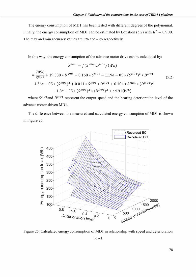
Chapter 5 Validation of the contributions in the case of TELMA platform
78
The energy consumption of MD1 has been tested with different degrees of the polynomial.
Finally, the energy consumption of MD1 can be estimated by Equation (5.2) with 𝑅2 = 0,988.
The max and min accuracy values are 8% and -6% respectively.
In this way, the energy consumption of the advance motor drive can be calculated by:
𝐸𝑀𝐷1 = 𝑓(𝑆𝑀𝐷1, 𝐷𝑀𝐷1) (𝑊ℎ)
=7856
𝑆𝑀𝐷1+ 19.538 ∗ 𝐷𝑀𝐷1 + 0.168 ∗ 𝑆𝑀𝐷1 − 1.19𝑒 − 05 ∗ (𝑆𝑀𝐷1)2 ∗ 𝐷𝑀𝐷1
−4.36𝑒 − 05 ∗ (𝑆𝑀𝐷1)2 + 0.011 ∗ 𝑆𝑀𝐷1 ∗ 𝐷𝑀𝐷1 + 0.104 ∗ 𝑆𝑀𝐷1 ∗ (𝐷𝑀𝐷1)2
+1.8𝑒 − 05 ∗ (𝑆𝑀𝐷1)2 ∗ (𝐷𝑀𝐷1)2 + 44.91(𝑊ℎ)
(5.2)
where 𝑆𝑀𝐷1and 𝐷𝑀𝐷1 represent the output speed and the bearing deterioration level of the
advance motor-driven MD1.
The difference between the measured and calculated energy consumption of MD1 is shown
in Figure 25.
Figure 25. Calculated energy consumption of MD1 in relationship with speed and deterioration
level
Chapter 5 Validation of the contributions in the case of TELMA platform
79
In order to ensure the synchronized speed between the two motors, the running speed is
controlled by PLC controllers. To maintain the useful output of system, the speed of roller may
be increased to perform more operation to complement the waste output to maintain the
productivity of punching function, for example, the slip between the roller the steel strip will
impact the number of steel sheet can be punched. The controller can impact the real operating
speed of motor driving system as following:
𝑆𝑀𝐷1 = 𝑆0𝑀𝐷1 + 𝜃 (
𝑟𝑜𝑢𝑛𝑑
𝑚𝑖𝑛𝑢𝑡𝑒𝑠),
(5.3)
Where 𝜃 presents the impact of controller accuracy to the operation speed of motor driven, 𝜃
can be seen as static impact factor. It is assumed that 𝜃 is subject to a degradation with 𝜃 = 𝑘 ∗ 𝑡
with 𝑘 is a coefficient. In this study we take 𝑘 = 7 for current state of controller of TELMA.
The output production capacity 𝑂𝑀𝐷1 during any period of time unit (from t to (t+1)) is
calculated as function of the setting speed 𝑆0𝑀𝐷1with rotation of roller seen as unit of output of
MD1. The ratio between rotation of motor and rotation of roller in the ideal case is fixed by the
ratio of gearbox and bell-driver system. In case of TELMA, we can used this ratio to calculate
output production capacity 𝑂𝑀𝐷1 from the setting speed 𝑆0𝑀𝐷1 for each one hour of operation:
𝑂𝑀𝐷1 = 60 ∗𝑆0
𝑀𝐷1
2500 (𝑟𝑜𝑢𝑛𝑑), (5.4)
where 𝑆0𝑀𝐷1 is setting speed of MD1 for each production mode.
Based on the results obtained by Equations (3.1), (5.2) and (5.4), we can use the following
equation to calculate EEI of MD1:
EEIMD1 =EMD1
OMD1 (Wh/round)
=32.7𝑒 + 04
𝑆𝑀𝐷1 ∗ 𝑆0𝑀𝐷1 +
814 ∗ 𝐷𝑀𝐷1
𝑆0𝑀𝐷1 + 7 ∗
𝑆𝑀𝐷1
𝑆0𝑀𝐷1
−49.59𝑒 − 05 ∗(𝑆𝑀𝐷1)2 ∗ 𝐷𝑀𝐷1
𝑆0𝑀𝐷1 − 18.16𝑒 − 04 ∗
(𝑆𝑀𝐷1)2
𝑆0𝑀𝐷1
+0.458 ∗𝑆𝑀𝐷1 ∗ 𝐷𝑀𝐷1
𝑆0𝑀𝐷1 + 4.33 ∗
𝑆𝑀𝐷1 ∗ (𝐷𝑀𝐷1)2
𝑆0𝑀𝐷1
+75𝑒 − 05 ∗(𝑆𝑀𝐷1)2 ∗ (𝐷𝑀𝐷1)2
𝑆0𝑀𝐷1 +
1871
𝑆0𝑀𝐷1 (Wh/round)
(5.5)

Chapter 5 Validation of the contributions in the case of TELMA platform
80
EEI of MD1 in relationship with the output speed and the deterioration level according to
Equation (5.5) is shown in Figure 26. The higher operating-speed of motors and/or the higher
level of bearing deterioration, the higher values of EEI can be calculated/recorded. The
calculated EEI values and recorded EEI values for MD1 are very close; it means that the EEI
model can be accepted with the sufficient accuracy at function level.
As the two motors are identical, the energy consumption, the useful output and EEI of MD2
can be calculated by equations:
𝐸𝑀𝐷2 = 𝑓(𝑆𝑀𝐷2, 𝐷𝑀𝐷2) (𝑊ℎ)
=7856
𝑆𝑀𝐷2+ 19.538 ∗ 𝐷𝑀𝐷2 + 0.168 ∗ 𝑆𝑀𝐷2 − 1.19𝑒 − 05 ∗ (𝑆𝑀𝐷2)2 ∗ 𝐷𝑀𝐷2
−4.36𝑒 − 05 ∗ (𝑆𝑀𝐷2)2 + 0.011 ∗ 𝑆𝑀𝐷2 ∗ 𝐷𝑀𝐷2 + 0.104 ∗ 𝑆𝑀𝐷2 ∗ (𝐷𝑀𝐷2)2
+1.8𝑒 − 05 ∗ (𝑆𝑀𝐷2)2 ∗ (𝐷𝑀𝐷2)2 + 44.91(𝑊ℎ)
(5.6)
𝑆𝑀𝐷2 = 𝑆0𝑀𝐷2 + 𝜃 (
𝑟𝑜𝑢𝑛𝑑
𝑚𝑖𝑛𝑢𝑡𝑒𝑠),
(5.7)
𝐸𝐸𝐼𝑀𝐷2 =𝐸𝑀𝐷2
𝑂𝑀𝐷2 (Wh/round)
=32.7𝑒 + 04
𝑆𝑀𝐷2 ∗ 𝑆0𝑀𝐷2 +
814 ∗ 𝐷𝑀𝐷2
𝑆0𝑀𝐷2 + 7 ∗
𝑆𝑀𝐷2
𝑆0𝑀𝐷2
−49.59𝑒 − 05 ∗(𝑆𝑀𝐷2)2 ∗ 𝐷𝑀𝐷2
𝑆0𝑀𝐷2 − 18.16𝑒 − 04 ∗
(𝑆𝑀𝐷2)2
𝑆0𝑀𝐷2
+0.458 ∗𝑆𝑀𝐷2 ∗ 𝐷𝑀𝐷2
𝑆0𝑀𝐷2 + 4.33 ∗
𝑆𝑀𝐷1 ∗ (𝐷𝑀𝐷1)2
𝑆0𝑀𝐷2
+75𝑒 − 05 ∗(𝑆𝑀𝐷2)2 ∗ (𝐷𝑀𝐷2)2
𝑆0𝑀𝐷2 +
1871
𝑆0𝑀𝐷2 (Wh/round)
(5.8)
With SMD2and DMD2 represent the output speed and the bearing deterioration level of
accumulator motor drive MD2.
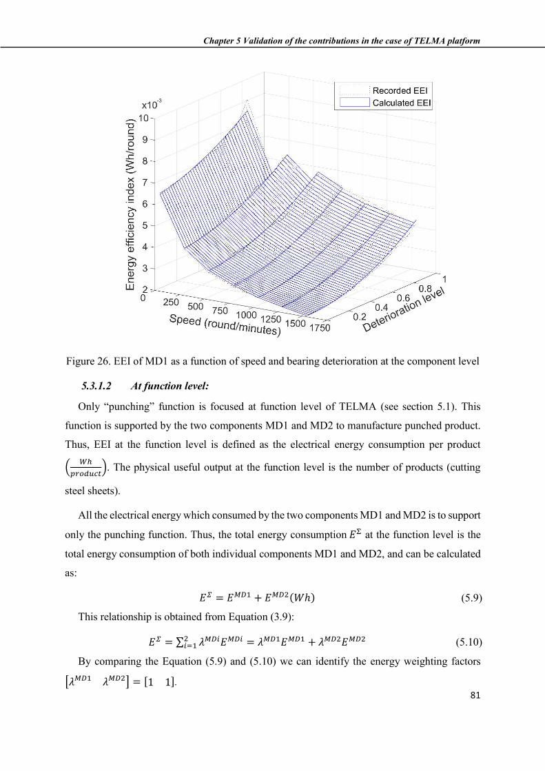
Chapter 5 Validation of the contributions in the case of TELMA platform
81
Figure 26. EEI of MD1 as a function of speed and bearing deterioration at the component level
5.3.1.2 At function level:
Only “punching” function is focused at function level of TELMA (see section 5.1). This
function is supported by the two components MD1 and MD2 to manufacture punched product.
Thus, EEI at the function level is defined as the electrical energy consumption per product
(𝑊ℎ
𝑝𝑟𝑜𝑑𝑢𝑐𝑡). The physical useful output at the function level is the number of products (cutting
steel sheets).
All the electrical energy which consumed by the two components MD1 and MD2 is to support
only the punching function. Thus, the total energy consumption 𝐸Σ at the function level is the
total energy consumption of both individual components MD1 and MD2, and can be calculated
as:
𝐸𝛴 = 𝐸𝑀𝐷1 + 𝐸𝑀𝐷2(𝑊ℎ) (5.9)
This relationship is obtained from Equation (3.9):
𝐸𝛴 = ∑ 𝜆𝑀𝐷𝑖𝐸𝑀𝐷𝑖2𝑖=1 = 𝜆𝑀𝐷1𝐸𝑀𝐷1 + 𝜆𝑀𝐷2𝐸𝑀𝐷2 (5.10)
By comparing the Equation (5.9) and (5.10) we can identify the energy weighting factors
[𝜆𝑀𝐷1 𝜆𝑀𝐷2] = [1 1].

Chapter 5 Validation of the contributions in the case of TELMA platform
82
In order to consider the output of the punching function as the production rate that is directly
related to the rotation of MD1 and MD2, it is important to note that to produce one product, the
rollers have to turn 25 rounds (this value is fixed according to the permanent physical connection
between roller and punch). Hence, the output weighting factors of separated MD1 and MD2 at
the function/system level can be expressed as follows:
[ωMD1 ωMD2] = [𝑂𝑀𝐷1
𝑂Σ
𝑂𝑀𝐷2
𝑂Σ] = [
25
1
25
1] (5.11)
The EEI of the considered “punching” function of the TELMA, 𝐸𝐸𝐼Σ, can be calculated by:
𝐸𝐸𝐼𝛴 = ∑ 𝜆𝑀𝐷𝑖𝜔𝑀𝐷𝑖𝐸𝐸𝐼𝑀𝐷𝑖2𝑖=1 = 1 ∗ 25 ∗ 𝐸𝐸𝐼𝑀𝐷1 + 1 ∗ 25 ∗ 𝐸𝐸𝐼𝑀𝐷2 (
𝑊ℎ
𝑝𝑟𝑜𝑑𝑢𝑐𝑡) (5.12)
5.3.2 Step 2: Prediction of the evolution of impact factors
From the identified impact factors of step 1 (section 4.2), the future operating conditions like
bearing deterioration levels, speed of motors and production plan should be forecasted.
5.3.2.1 At component level
On TELMA, a production program that is considered as a static factor and seen in advance
by using Markov processes is forecasted as shown in Figure 27.a. It is assumed that the
production schedule does not impact the deterioration process of two motors and that the bearing
deterioration behavior of MD1 and MD2 depends only on the time. A gamma stochastic process
is used to simulate the bearing damaging behavior of MD1 and MD2 [113]. Two parameters α
> 0 and β > 0 are taken and Gamma function 𝛤(𝛼) is defined by:
𝛤(𝛼) = ∫ 𝑢𝛼−1𝑒−𝑢𝑑𝑢∞
0
(5.13)
During (T𝑖−1 − t) period of time unit, the increment in the deterioration level of the
bearing x = (D(t) − D(T𝑖−1)) follows Gamma probability density with the shape parameter
α(t − T𝑖−1) and the scale parameter β as:
𝑓𝛼(𝑡−𝑇)(𝑥)=
𝛽
𝛤(𝛼(𝑡−T𝑖−1))(𝛽𝑥)𝛼(𝑡−T𝑖−1)−1(𝑒)−𝛽𝑥
(5.14)
The deterioration speed and its variance are 𝑘 = 𝛼/𝛽 and 𝑉𝑎𝑟[𝑥] = 𝛼/𝛽2 respectively. In
case of real data of bearings are recordable or available, the parameters (𝛼, 𝛽) of the bearing
deterioration model can be identified [196]. The parameters associated with the Gamma
deterioration model (based on the data of deterioration behaviors of MD1 and MD2) are
presented in Table 6. Each motor-driven system is considered failed when the deterioration level
reaches the 100% level.
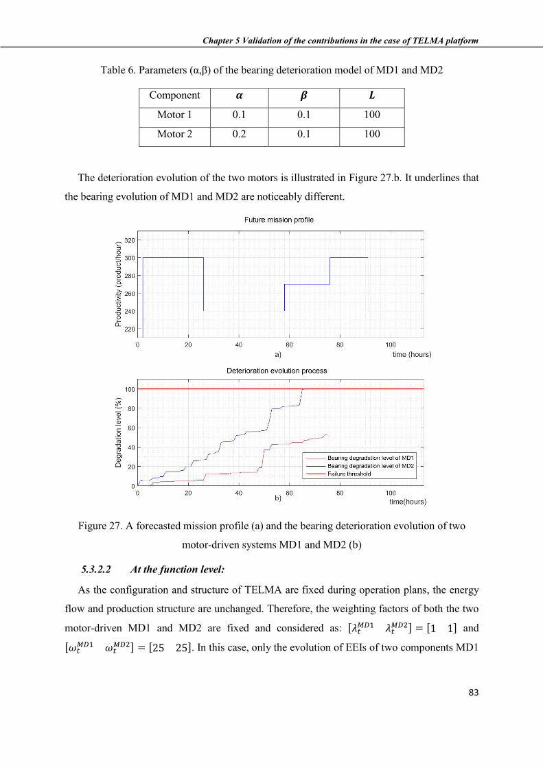
Chapter 5 Validation of the contributions in the case of TELMA platform
83
Table 6. Parameters (α,β) of the bearing deterioration model of MD1 and MD2
Component 𝜶 𝜷 𝑳
Motor 1 0.1 0.1 100
Motor 2 0.2 0.1 100
The deterioration evolution of the two motors is illustrated in Figure 27.b. It underlines that
the bearing evolution of MD1 and MD2 are noticeably different.
Figure 27. A forecasted mission profile (a) and the bearing deterioration evolution of two
motor-driven systems MD1 and MD2 (b)
5.3.2.2 At the function level:
As the configuration and structure of TELMA are fixed during operation plans, the energy
flow and production structure are unchanged. Therefore, the weighting factors of both the two
motor-driven MD1 and MD2 are fixed and considered as: [𝜆𝑡𝑀𝐷1 𝜆𝑡
𝑀𝐷2] = [1 1] and
[𝜔𝑡𝑀𝐷1 𝜔𝑡
𝑀𝐷2] = [25 25]. In this case, only the evolution of EEIs of two components MD1

Chapter 5 Validation of the contributions in the case of TELMA platform
84
and MD2 impact the changing of EEI value at function level 𝐸𝐸𝐼𝛴(𝑡). This leads to a final
formulation of EEI at the function level that can be determined by the following equation:
𝐸𝐸𝐼𝛴(𝑡) = ∑ 𝜆𝑡𝑀𝐷𝑖𝜔𝑡
𝑀𝐷𝑖𝐸𝑀𝐷𝑖(𝑡)
2
𝑖=1
= 1 ∗ 25 ∗ 𝐸𝐸𝐼𝑀𝐷1(𝑡) + 1 ∗ 25 ∗ 𝐸𝐸𝐼𝑀𝐷2(𝑡) (𝑊ℎ
𝑝𝑟𝑜𝑑𝑢𝑐𝑡)
(5.15)
Because the evolution of EEI for each motor-driven is different according to their
characteristic (deterioration speed, controller accuracy, etc.), the distribution of EEI at
“punching” function level can be totally different.
5.3.3 Step 3: Evaluation of the potential evolution of EEI and estimation of REEL
Based on the simulated productivity (see again Figure 27.a) and bearing deterioration
evolution, which are predicted in Step 2 (see section 4.3.2), EEI of MD1 and MD2 at the
component and function levels of TELMA can be estimated at any time point. EEI evolution at
the component/function levels of the platform TELMA is shown in Figure 28.
Figure 28. Evolution of EEI at the component level (a) and at the function level (b)
A limit value 𝐸𝐸𝐼𝑇ℎ𝑟𝑒𝑠ℎ𝑜𝑙𝑑 = 1030 (Wh/product) is given in advance as a threshold value at
the function level. TELMA platform is seen to work in the energy inefficient zone when its EEI
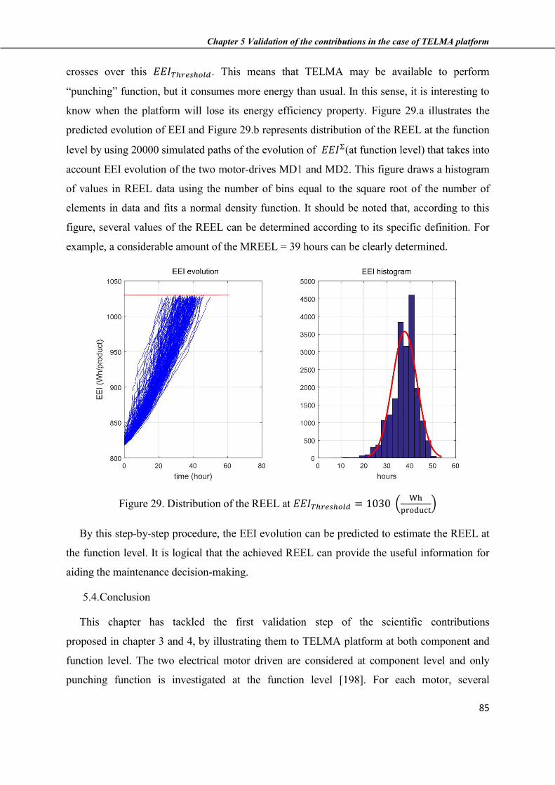
Chapter 5 Validation of the contributions in the case of TELMA platform
85
crosses over this 𝐸𝐸𝐼𝑇ℎ𝑟𝑒𝑠ℎ𝑜𝑙𝑑. This means that TELMA may be available to perform
“punching” function, but it consumes more energy than usual. In this sense, it is interesting to
know when the platform will lose its energy efficiency property. Figure 29.a illustrates the
predicted evolution of EEI and Figure 29.b represents distribution of the REEL at the function
level by using 20000 simulated paths of the evolution of 𝐸𝐸𝐼Σ(at function level) that takes into
account EEI evolution of the two motor-drives MD1 and MD2. This figure draws a histogram
of values in REEL data using the number of bins equal to the square root of the number of
elements in data and fits a normal density function. It should be noted that, according to this
figure, several values of the REEL can be determined according to its specific definition. For
example, a considerable amount of the MREEL = 39 hours can be clearly determined.
Figure 29. Distribution of the REEL at 𝐸𝐸𝐼𝑇ℎ𝑟𝑒𝑠ℎ𝑜𝑙𝑑 = 1030 (Wh
product)
By this step-by-step procedure, the EEI evolution can be predicted to estimate the REEL at
the function level. It is logical that the achieved REEL can provide the useful information for
aiding the maintenance decision-making.
5.4. Conclusion
This chapter has tackled the first validation step of the scientific contributions
proposed in chapter 3 and 4, by illustrating them to TELMA platform at both component and
function level. The two electrical motor driven are considered at component level and only
punching function is investigated at the function level [198]. For each motor, several

Chapter 5 Validation of the contributions in the case of TELMA platform
86
experimentations on the energy consumption as a function of the production plan (static impact
factor) and the deterioration state of bearing (dynamic impact factor) are carried out. Based on
the recorded data, an EEI model (including two formalization of energy consumption and output)
is provided at both component and function level. For the prognostic implementation for
EEI/REEL prediction, the evolution of the bearing is described by a Gamma process. The
achieved results demonstrate that the EEI evolution can be predicted both at the component level
and at the function level for specific experiment.
The study developed in this chapter highlights the potential achievement of our proposals and
shows the added value of the proposed EEI and REEL concept.

Chapter 6 Use of EE for CBM maintenance decision-making
87
Chapter 6 Use of EE for CBM maintenance decision-making
6.1. Introduction
This chapter describes our contribution on the use of EE for condition-based maintenance
which is the scientific issue n°4 pointed out in chapter 2. Firstly, a qualitative study on the use
of EEI for decision-making is investigated. Then a detailed development of EEI for condition-
based maintenance is presented. In fact, the main idea is to use EEI as the decision indicator for
selecting a component or a group of several components to be preventively maintained. Two
kinds of preventive decision rules are proposed. A cost model is then proposed for finding the
optimal decision parameters. Moreover, a classical CBM, in which the preventive decision-
making is based on a conventional degradation indicator, is also extended by considering not
only the maintenance cost but also the energy cost in the way to compare the proposed EEI-
based CBM approach with the conventional (extended) one. The comparison step is developed
on the case study of TELMA platform allowing to assess the impact of EEI on the existing CBM
policy and to conclude on the interest of EEI for CBM decision-making in terms of cost and
efficiency.
6.2. General dicussions on EEI indicator for decision-making
Before using EEI as a main indicator in CBM maintenance decision-making, we want just to
underline several principal characteristics of EEI (in addition to the discussion already done in
chapter 2).
EEI is a universal indicator for different decision-making levels
Measuring business performance is the top priority for most of industrial stakeholders. The
higher level of decision-making is, the more universal decision-indicators should be. It means
that decisional indicators can provide the economical information for higher decision-making
levels. In CBM framework, conventional degradation indicators such as crack, noise, etc. are not
easy to transform to financial indicators while EEI can be easily transferred to the monetary. EEI
threshold has to be defined to fulfil specific business goals and objectives such as supporting

Chapter 6 Use of EE for CBM maintenance decision-making
88
environment certificate, eco-maintenance – “green production” [199]. It can be directly linked
to the overall goals of the company (especially at strategic level).
EEI provides a clear vision for decision-makers:
Firstly, energy efficiency is supported by various conceptual/theory framework (codes,
standard, guideline, etc.) [47], [57], [150]. [158], [200]. [16], [87], [116]. These proposed works
help to measure, monitoring and evaluate EE performance at different application domains in
comparison with lack of framework for conventional indicators.
Secondly, EEI is understandable for any decision-maker while most of conventional
indicators are quite complicated in representing the health status of component/system. The EEI
value can be measureable by, for example, implementing energy efficiency audit. Technical
operators usually know what impact factors should be measured (related to energy consumption,
output), how it’s being calculated and finally what actions can positively impact EEI [201].
Low inspection cost:
In reality, energy management systems (EMS) are implemented in almost industrial system
to control and regulate the machines in order to improve its energy efficiency performance
[202]–[204]. Therefore, EEI can be monitored with an inspection cost [193]. While to monitor
conventional deterioration indicators, additional measurements and many computations may be
required [97]. As a consequence, monitoring/acquiring the data of conventional indicators may
be more complicated, expensive, and impractical for actual application [205], [206].
Furthermore, physical inspection duration may be longer than EEI inspection duration. This may
lead to an addition consequence such as low production capacity, waste labor forces. Moreover,
under the development of IT technology, the energy data can be continuously collected over time
[207], [208]. This can help to optimally update online the maintenance decision-making process
adapting with real operation situations.
6.3. EEI-based CBM maintenance
It is assumed, in this CBM study, that both corrective and preventive maintenance are possible
for each component and these maintenance actions can bring the maintained component to be a
new one (replacement action). We also suppose that the maintenance duration can be neglected.
Chapter 6 Use of EE for CBM maintenance decision-making
89
6.3.1. Maintenance decision rules
It is assumed that EEI of each component is monitored at each regular time point 𝑇𝑖 = 𝑖 ∗ ∆𝑇
(∆𝑇 is a decision parameter to be optimized; i=1,2,…). Each energy efficiency inspection costs
𝐶𝑖𝑛𝐸 .
Between two consecutive inspection times, if component j fails, a corrective maintenance
action is performed at the next inspection date with a corrective maintenance cost 𝐶𝑐𝑗 . If the
failure of component j leads to a shutdown of the function/system, a downtime cost 𝐶𝑑. 𝑑𝑖(𝑡)
(with 𝐶𝑑is the downtime cost rate and 𝑑𝑖 is the downtime duration between [𝑇𝑖−1, 𝑇𝑖]) is added.
For preventive maintenance operations, we consider herein two main preventive maintenance
policies: individual maintenance and grouping maintenance. This consideration leads to a first
part of the scientific issue n°4 which is related to using EEI value as condition of CBM strategy.
6.3.1.1. Individual maintenance policy:
At each regular time point 𝑇𝑖, a preventive maintenance on component j is triggered if its EEI
value monitored, 𝐸𝐸𝐼𝑗𝑇𝑖
, is higher than a threshold denoted 𝐸𝐸𝐼𝑗𝑃𝑟𝑒_𝑡ℎ𝑟𝑒𝑠ℎ𝑜𝑙𝑑 which is also a
decision parameter to be optimized. In that way, the decision rules for each component at each
regular time point is the following:
- if 𝐸𝐸𝐼𝑗𝑇𝑖
< 𝐸𝐸𝐼𝑗𝑃𝑟𝑒_𝑡ℎ𝑟𝑒𝑠ℎ𝑜𝑙𝑑 then no maintenance action is performed;
- if 𝐸𝐸𝐼𝑗𝑇𝑖
≥ 𝐸𝐸𝐼𝑗𝑃𝑟𝑒_𝑡ℎ𝑟𝑒𝑠ℎ𝑜𝑙𝑑 then a preventive maintenance action on component j is
performed. A preventive cost 𝐶𝑝𝑗 has to be paid.
The illustration of maintenance decision rules is shown in Figure 30.
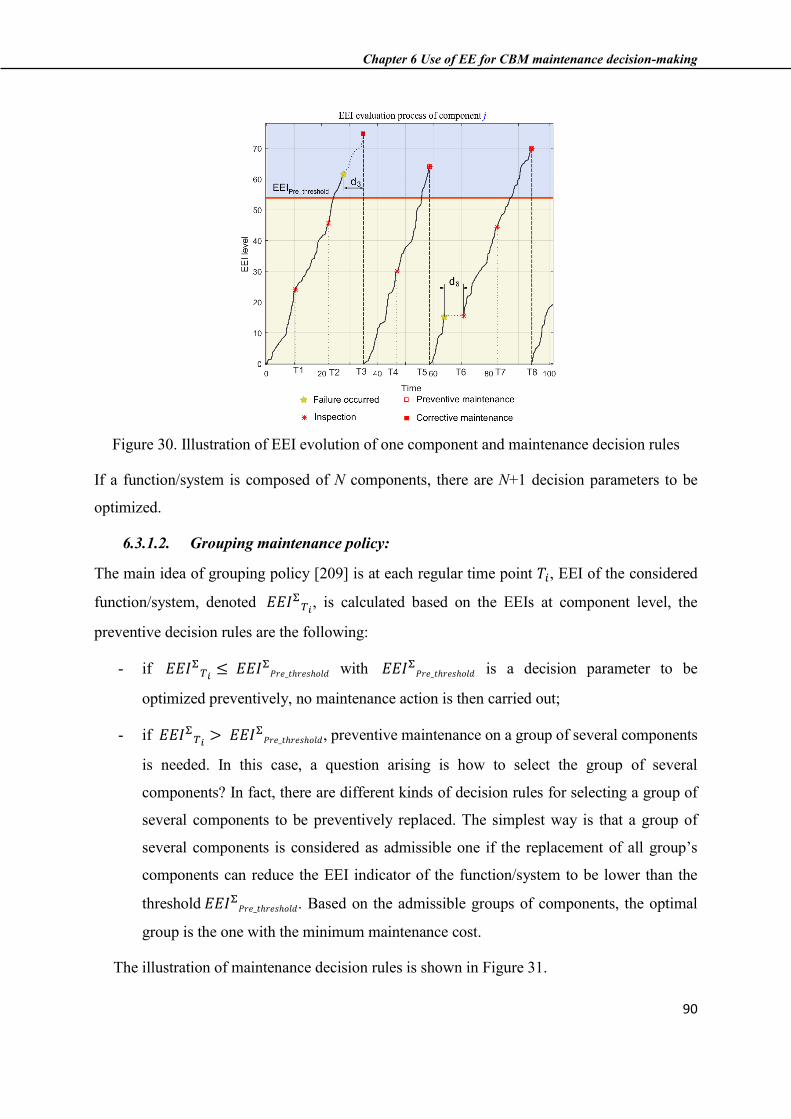
Chapter 6 Use of EE for CBM maintenance decision-making
90
Figure 30. Illustration of EEI evolution of one component and maintenance decision rules
If a function/system is composed of N components, there are N+1 decision parameters to be
optimized.
6.3.1.2. Grouping maintenance policy:
The main idea of grouping policy [209] is at each regular time point 𝑇𝑖, EEI of the considered
function/system, denoted 𝐸𝐸𝐼Σ𝑇𝑖
, is calculated based on the EEIs at component level, the
preventive decision rules are the following:
- if 𝐸𝐸𝐼Σ𝑇𝑖
≤ 𝐸𝐸𝐼Σ𝑃𝑟𝑒_𝑡ℎ𝑟𝑒𝑠ℎ𝑜𝑙𝑑 with 𝐸𝐸𝐼Σ
𝑃𝑟𝑒_𝑡ℎ𝑟𝑒𝑠ℎ𝑜𝑙𝑑 is a decision parameter to be
optimized preventively, no maintenance action is then carried out;
- if 𝐸𝐸𝐼Σ𝑇𝑖
> 𝐸𝐸𝐼Σ𝑃𝑟𝑒_𝑡ℎ𝑟𝑒𝑠ℎ𝑜𝑙𝑑, preventive maintenance on a group of several components
is needed. In this case, a question arising is how to select the group of several
components? In fact, there are different kinds of decision rules for selecting a group of
several components to be preventively replaced. The simplest way is that a group of
several components is considered as admissible one if the replacement of all group’s
components can reduce the EEI indicator of the function/system to be lower than the
threshold 𝐸𝐸𝐼Σ𝑃𝑟𝑒_𝑡ℎ𝑟𝑒𝑠ℎ𝑜𝑙𝑑. Based on the admissible groups of components, the optimal
group is the one with the minimum maintenance cost.
The illustration of maintenance decision rules is shown in Figure 31.

Chapter 6 Use of EE for CBM maintenance decision-making
91
Figure 31. Illustration of EEI evolution of system and maintenance decision rules
According to the group maintenance policy, only two decision parameters are required
6.3.1.3. Cost model
To find the optimal decision parameters, cost is used as a main criterion. In that way, the
long-run expected cost per useful output unit, is used. The following development is applied for
both the individual maintenance and grouping maintenance policies.
The cumulative total cost for the period (0-t] is expressed as:
𝑇𝑜𝑡𝑎𝑙𝐶𝑡 = 𝑀𝐶𝑡 + 𝐸𝐶𝑡 (6.1)
where:
- 𝑀𝐶𝑡 is the cumulative maintenance cost which can be calculated by
𝑀𝐶𝑡 = CI𝑡 + CP𝑡 + CC𝑡 + CD𝑡 (6.2)
where: CI𝑡 , CP𝑡, CC𝑡 and CD𝑡 are respectively the costs associated with to EEI
inspection, preventive maintenance, corrective maintenance and downtime duration
during the period (0-t].

Chapter 6 Use of EE for CBM maintenance decision-making
92
- 𝐸𝐶𝑡 is the cumulative energy cost and can be calculated as
𝐸𝐶𝑡 = 𝐸𝑝. ∫ ∑ 𝐸𝑗(𝑥)
𝑁
𝑖=1
𝑡
0
𝑑𝑥 (6.3)
With 𝐸𝑝 represents the energy price and 𝐸𝑖(𝑥) is the energy consumption during one
time unit (from (x-1) to x) of component j. 𝐸𝑖(𝑡) depends not only on the
state/deterioration level of component j but also on the other impact factors (such as
product capacity, waste rate).
𝐸𝑗(𝑡) = 𝑓(𝑡, 𝑋𝑡𝑗, 𝑥(𝑡))
(6.4)
Where 𝑋𝑡𝑗 is the state/degradation level of component j and x(𝑡) is the set of impact factors
during one time unit (from t to (t+1)). It is important to recall that component j is considered as
failed if its deterioration level is not lower than a critical threshold: 𝑋𝑡𝑗
≥ 𝐿𝑗 .
The cumulative useful output during the period (0 t] is written as:
∅(𝑡) = ∫ 𝑂(𝑥)𝑑𝑥𝑡
0
(6.5)
The long run global cost per useful output unit is the following:
𝐶𝑂 = lim𝑡→∞
𝑇𝑜𝑡𝑎𝑙𝐶𝑡
∅(𝑡) (6.6)
By using the renewal theory [210], we obtain:
𝐶𝑂 =𝐸[𝑇𝑜𝑡𝑎𝑙𝐶𝐻]
𝐸[∅(𝐻)] (6.7)
with 𝐻 is the first replacement date. Stochastic Monte Carlo simulation (on MATLAB tools)
is used to evaluate this cost criterion. To do so, for each value of decision parameters, the
corresponding total cost per useful output unit is calculated. To ensure that the convergence of
maintenance cost rate is reached, a large number of simulation realizations (each realization
simulates one life cycle of the system) must be done. The optimal value of the decision
parameters are given when the total cost per useful output searches its minimum value [211].
6.3.2. Extension of a classical CBM policy
To highlight the performance of the proposed EEI-CBM based maintenance, a classical
CBM, namely (M,T) policy in which a conventional deterioration is used as a main decisional
Chapter 6 Use of EE for CBM maintenance decision-making
93
indicator is extended by integrating the energy consumption cost. The comparison between the
extended (M,T) CBM and EEI-based CBM tackles the second part of the scientific issue n°4
which related to assess the benefits of EEI-based CBM strategy.
6.3.2.1. Maintenance decision rules
It is assumed that the deterioration level of each component is inspected at regular each
regular time point 𝑇𝑖 = 𝑖 ∗ ∆𝑇 (∆𝑇 is a decision parameter to be optimized; i=1,2,…). Each
deterioration inspection costs 𝐶𝑖𝑛𝐷 with (𝐶𝑖𝑛
𝐷 ≥ 𝐶𝑖𝑛𝐸 ).
Between two consecutive inspection times, if component j fails, a corrective maintenance
action is performed at the next inspection date with a corrective maintenance cost 𝐶𝑐𝑗 . If the
failure of component j leads to a shutdown of the function/system, a downtime cost 𝐶𝑑. 𝑑𝑖(𝑡)
(with 𝐶𝑑is the downtime cost rate and 𝑑𝑖 is the downtime duration between [𝑇𝑖−1, 𝑇𝑖]) is added.
Concerning preventive maintenance, unlike EEI indicator, the deterioration indicator can be
only defined at component level, as a consequence, a unique main maintenance policy is herein
considered: individual maintenance. The decision rules for component j are the following:
- if 𝑋𝑗𝑇𝑖
< 𝑀𝑗 then no maintenance action is performed. 𝑀𝑗 is the preventive threshold
to be optimized;
- if 𝑋𝑗𝑇𝑖
≥ 𝑀𝑗 then a preventive maintenance action on component j is performed. A
preventive cost 𝐶𝑝𝑗 has to be paid.
Figure 32 presents the behavior of single component with its evolution of deterioration level
with maintenance actions.

Chapter 6 Use of EE for CBM maintenance decision-making
94
Figure 32. Behaviour of the maintained component under the (M,T) policy
According to the policy, there are N+1 decision parameters (∆𝑇, 𝑀1, 𝑀2, … , 𝑀N) to be
optimized.
6.3.2.2. Cost model with consideration of energy consumption cost
By considering the energy cost in the total cost to operate the industrial system.
The long run global cost per useful output unit is the following:
𝐶𝑂 = lim𝑡→∞
𝑇𝑜𝑡𝑎𝑙𝐶𝑡
O(𝑡)
(6.8)
with:
𝑇𝑜𝑡𝑎𝑙𝐶𝑡 = 𝑀𝐶𝑡 + 𝐸𝐶𝑡 (6.9)
where:
- 𝑀𝐶𝑡 is the cumulative maintenance cost which can be calculated by
𝑀𝐶𝑡 = CI𝑡 + CP𝑡 + CC𝑡 + CD𝑡 (6.10)

Chapter 6 Use of EE for CBM maintenance decision-making
95
where: CI𝑡 , CP𝑡 , CC𝑡 and CD𝑡 are respectively the costs related to degradation inspection,
preventive maintenance, corrective maintenance and downtime duration during the period
(0-t].
- 𝐸𝐶𝑡 is the cumulative energy cost and can be calculated as
𝐸𝐶𝑡 = 𝐸𝑝. ∫ ∑ 𝐸𝑗(𝑥)
𝑁
𝑖=1
𝑡
0
𝑑𝑥 (6.11)
The cumulative useful output during the period (0 t] is written as:
∅(𝑡) = ∫ 𝑂(𝑥)𝑑𝑥𝑡
0
(6.12)
The long run global cost per useful output unit is the following:
𝐶𝑂 = lim𝑡→∞
𝑇𝑜𝑡𝑎𝑙𝐶𝑡
∅(𝑡) (6.13)
By using the renewal theory [210], we obtain:
𝐶𝑂 =𝐸[𝑇𝑜𝑡𝑎𝑙𝐶𝐻]
𝐸[∅(𝐻)] (6.14)
Stochastic Monte Carlo simulation is used to evaluate this cost criterion. To do so, for each
value of decision parameters (∆𝑇, 𝑀1, 𝑀2, … , 𝑀N) the corresponding cost per useful output unit
is calculated.
The optimal value of the inspection period and the preventive thresholds are given by
minimizing the total cost per useful output.
6.4. Implementation platform TELMA
The proposed EE-based CBM maintenance policy is applied on TELMA platform dedicated
to e-maintenance (as described in section 5.2). The proposed EE-based CBM maintenance and
the (M,T) policy are applied for only one motor-driven MD1. The speed of MD1 is set to 𝑆0𝑀𝐷1 =
300 (rpm). The data concerning the deterioration behavior and the energy consumption of MD1
discussed in Section 5.2 is reconsidered. Table 7 reports the cost data (computed in cost unit –
CU).

Chapter 6 Use of EE for CBM maintenance decision-making
96
Table 7. Energy and maintenance simulation parameter
𝐸𝑝 𝐶𝑝 𝐶𝑐 𝐶𝑑 𝑐𝑖𝑛𝐸 𝑐𝑖𝑛
𝐷
0.025 (CU/𝑊ℎ) 100 (CU) 150 (CU) 100 (CU) 1 (CU) 10 (CU)
6.4.1. Maintenance optimization for MD1
6.4.1.1. EEI-based CBM maintenance
Figure 33 shows the surface of cost rate of the EEI-based policy as a function of the decision
parameters (∆𝑇, 𝐸𝐸𝐼𝑃𝑟𝑒_𝑡ℎ𝑟𝑒𝑠ℎ𝑜𝑙𝑑). The optimum value of the decision parameters are
𝐸𝐸𝐼𝑃𝑟𝑒_𝑡ℎ𝑟𝑒𝑠ℎ𝑜𝑙𝑑∗ = 25 (𝑊ℎ/𝑟𝑜𝑢𝑛𝑑) and ∆𝑇∗ = 9 (ℎ𝑜𝑢𝑟𝑠) with the minimum global cost per
product unit 𝐶𝑂∗(. ) = 0.74 (𝐶𝑈/𝑟𝑜𝑢𝑛𝑑).
Figure 33. Cost rate surface of the EEI-based CBM maintenance
6.4.1.2. (M,T) maintenance policy
In the same manner, the total cost including maintenance and energy cost per product unit is
calculated for each set of the decision parameters (∆𝑇, 𝑀). Figure 34 shows the shape of the cost
rate of the (M,T)-based CBM policy for MD1.

Chapter 6 Use of EE for CBM maintenance decision-making
97
Figure 34. Cost rate surface of the (M,T)-based CBM policy
The optimal decision parameters are the maintenance threshold 𝑀∗ = 43 and inspection
period ∆𝑇∗ = 24 (ℎ𝑜𝑢𝑟𝑠) with 𝐶𝑂∗(. ) = 0.81 (𝐶𝑈/𝑟𝑜𝑢𝑛𝑑). When compared to the proposed
EEI-based policy, the (M,T) maintenance policy leads to a higher cost rate. This can be explained
by the fact that the inspection cost for EEI is lower than the inspection cost of bearing
deterioration indicator and more importantly the potential evolution of EEI vary less than the
bearing deterioration indicator do. This leads to a higher performance of the decision-making
based on the EEI. As example, Figure 35.a shows the distribution of EEI and the bearing
deterioration indicator at preventive maintenance time which is based on EEI level
(𝐸𝐸𝐼𝑃𝑟𝑒_𝑡ℎ𝑟𝑒𝑠ℎ𝑜𝑙𝑑 = 25 (𝑊ℎ/𝑟𝑜𝑢𝑛𝑑)). When the preventive maintenance decision is based on the
bearing deterioration level (𝑀 = 43), the distribution of EEI and the bearing deterioration
indicator are shown in Figure 35.b. It is found that the variation of EEI is less than that of the
bearing deterioration indicator.

Chapter 6 Use of EE for CBM maintenance decision-making
98
Figure 35. Distribution of condition indicators at preventive maintenance time which is based
on a) EEI level and b) conventional deterioration level
It should be noticed that the performance of EEI-based CBM may depends on the value of
other parameters.
6.4.2. Sensitivity analyses
From the previous results, the following sensitivity analyses are investigated for both EEI-
based CBM and (M,T) policy:
- Sensitivity analysis to the inspection cost
- Sensitivity analysis to the preventive maintenance cost
- Sensitivity analysis to the energy cost rate
- Sensitivity analysis to the bearing deterioration behavior
6.4.2.1. Sensitivity analysis to inspection cost
In this study, the inspection cost (𝐶𝑖𝑛𝐸 for EEI-based maintenance and 𝐶𝑖𝑛
𝐷 for (M,T) policy)
varies from 1 to 120. The obtained results in Table 8 show that the proposed EEI-based CBM
provides a lower total cost than the (M,T) policy.
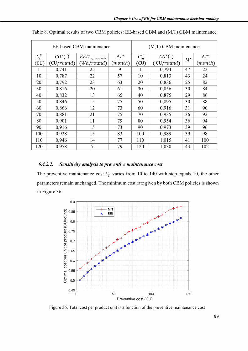
Chapter 6 Use of EE for CBM maintenance decision-making
99
Table 8. Optimal results of two CBM policies: EE-based CBM and (M,T) CBM maintenance
EE-based CBM maintenance (M,T) CBM maintenance
𝐶𝑖𝑛𝐸
(CU) 𝐶𝑂∗(. )
(CU/𝑟𝑜𝑢𝑛𝑑) 𝐸𝐸𝐼𝑃𝑟𝑒_𝑡ℎ𝑟𝑒𝑠ℎ𝑜𝑙𝑑
∗ (𝑊ℎ/𝑟𝑜𝑢𝑛𝑑)
∆𝑇∗ (𝑚𝑜𝑛𝑡ℎ)
𝐶𝑖𝑛𝐷
(CU) 𝐶𝑂∗(. )
( CU/𝑟𝑜𝑢𝑛𝑑) 𝑀∗ ∆𝑇∗ (𝑚𝑜𝑛𝑡ℎ)
1 0,741 25 9 1 0,794 47 22 10 0,787 22 57 10 0,813 43 24 20 0,792 23 63 20 0,836 25 82 30 0,816 20 61 30 0,856 30 84 40 0,832 13 65 40 0,875 29 86 50 0,846 15 75 50 0,895 30 88 60 0,866 12 73 60 0,916 31 90 70 0,881 21 75 70 0,935 36 92 80 0,901 11 79 80 0,954 36 94 90 0,916 15 73 90 0,973 39 96 100 0,928 15 83 100 0,989 39 98 110 0,946 14 77 110 1,015 41 100 120 0,958 7 79 120 1,030 43 102
6.4.2.2. Sensitivity analysis to preventive maintenance cost
The preventive maintenance cost 𝐶𝑝 varies from 10 to 140 with step equals 10, the other
parameters remain unchanged. The minimum cost rate given by both CBM policies is shown
in Figure 36.
Figure 36. Total cost per product unit is a function of the preventive maintenance cost
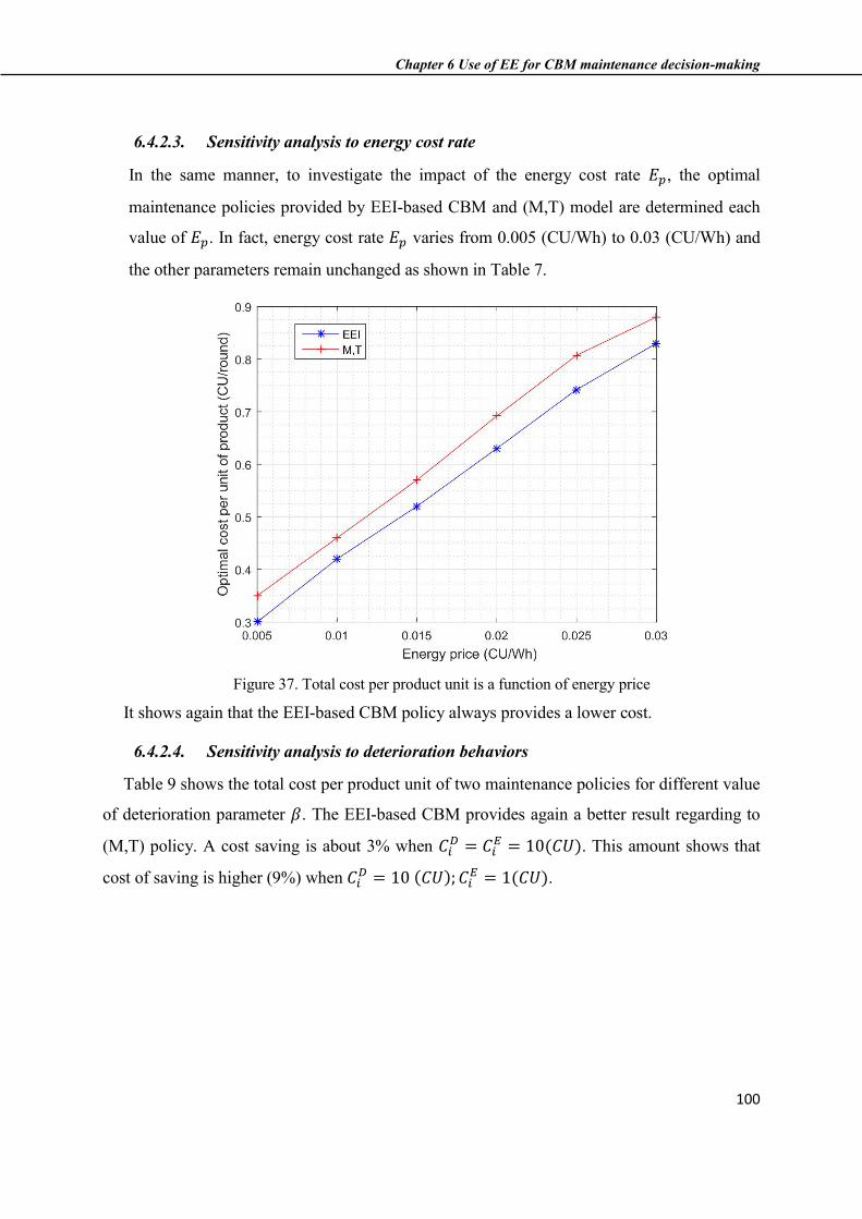
Chapter 6 Use of EE for CBM maintenance decision-making
100
6.4.2.3. Sensitivity analysis to energy cost rate
In the same manner, to investigate the impact of the energy cost rate 𝐸𝑝, the optimal
maintenance policies provided by EEI-based CBM and (M,T) model are determined each
value of 𝐸𝑝. In fact, energy cost rate 𝐸𝑝 varies from 0.005 (CU/Wh) to 0.03 (CU/Wh) and
the other parameters remain unchanged as shown in Table 7.
Figure 37. Total cost per product unit is a function of energy price
It shows again that the EEI-based CBM policy always provides a lower cost.
6.4.2.4. Sensitivity analysis to deterioration behaviors
Table 9 shows the total cost per product unit of two maintenance policies for different value
of deterioration parameter 𝛽. The EEI-based CBM provides again a better result regarding to
(M,T) policy. A cost saving is about 3% when 𝐶𝑖𝐷 = 𝐶𝑖
𝐸 = 10(𝐶𝑈). This amount shows that
cost of saving is higher (9%) when 𝐶𝑖𝐷 = 10 (𝐶𝑈); 𝐶𝑖
𝐸 = 1(𝐶𝑈).

Chapter 6 Use of EE for CBM maintenance decision-making
101
Table 9. Minimum total cost rate cost with different deterioration behaviours
𝐶𝑂∗(. ) (CU/𝑟𝑜𝑢𝑛𝑑)
EEI-based CBM (M,T) based CBM 𝐶𝑖
𝐸 = 1 (CU) 𝐶𝑖𝐸 = 10 (CU) 𝐶𝑖
𝐷 = 10 (CU)
1,00 0,621 0,623 0,625
0,80 0,624 0,631 0,635
0,50 0,631 0,642 0,647
0,25 0,655 0,661 0,665
0,20 0,668 0,694 0,704
0,10 0,741 0,787 0,813
The results show the larger variation of the deterioration process (small value of 𝜷) the more
cost saving provided by the proposed EEI-based CBM is.
6.5. Conclusion
In this chapter, a novel CBM maintenance is introduced by considering EEI as the decisional
indicator for preventive maintenance-decision making. This EEI-based CBM tackles the issue
related to integrate EE in CBM strategies (scientific issue n°4 in chapter 2). Two kinds of
preventive maintenance rules are proposed to optimally select appropriate components to be
preventively replaced. The first one, namely individual maintenance for which each component
is individually selected according to its EEI level, leads to a large number of decision parameters
((N+1) decision parameters for a function/system composed of N components). For the second
preventive maintenance policy, called grouping maintenance, a group of several components are
jointly selected when the EEI of the whole function/system is lower than a prefixed EEI
threshold. Thanks to the EEI consideration, only two decision parameters are needed whatever
the number of components supporting the function/system.
To highlight the performance of the proposed EEI-based CBM maintenance, a classical CBM
maintenance in which the preventive decision on each component is based on its physical
deterioration level is also extended by integrating the energy cost into the existing cost model. It
is important to note that the extended CBM maintenance, called (M,T) maintenance policy, lead
to a large number of decision parameters to be optimized (each component requires one decision
parameter).

Chapter 6 Use of EE for CBM maintenance decision-making
102
Both the proposed EEI-based CBM and the (M,T) policy are applied for one motor of the
platform TELMA. The various numerical studies show that the proposed EEI-based policy
provides a better result (lower cost per product unit).
103
General conclusion
This core idea defended in this thesis is related to the necessary evolution of maintenance and
more precisely CBM strategies for integrating Energy Efficiency (EE) in terms of EE Indicator
(EEI) and REEL concepts, in the decision making phase.
These two EE concepts are representative of sustainability requirements which are required
to be achieved now by the industrial system to face not only with economic, but also societal
and environmental challenges (three pillars). In that way, the thesis addressed several issues
which are related to the foundation of these concepts, their formulation, their evolutions in terms
of value trends by considering dynamics of the system, their consideration in CBM, their first
step of validation on a specific case …
From these issues, it is promoted several contributions:
- The first ones developed in Chapter 3 are related to the generic definition of EEI for
different abstraction levels and materialized by its two properties: energy consumption
and physical useful output. Then a generic EEI formulation, usable at each level, is
proposed. This formulation is described as the ratio between these two properties in which
time-dependent factors (called static and dynamic factors) are considered. Formulation
can serve latter for a specific manufacturing system to calculate EEI value and also EEI
evolution (due to the time-dependent factors). Based on this EEI evolution, a novel
concept named REEL (Remaining Energy-Efficient Lifetime) is introduced as the
foundation of EEP (to assess the remaining time before a component/function/system lost
its energy properties under a limit threshold),
- The second ones developed in Chapter 4 are related to a generic approach for
implementing different steps required to use the generic formulation for EEI calculation
on a specific manufacturing system and then to assess REEL. This generic approach is
structured on three steps (Figure 14): (1) identification, at each abstraction level of the
selected system, of the two EEI properties (energy consumption, useful manufactured
product) but also of the impact factors. It leads to isolate or create models integrating
these factors and supporting the properties modelling to obtain EEI models (specific
formulations). (2) Implementation of prognostic method the most appropriated for
104
predicting the evolution of each impact factor. (3) Re-integration in the EEI model of the
impact factors evolutions, to be able to track EEI evolution allowing to assess the REEL.
- The last ones developed in Chapter 6 are addressed, first, the proposal of a new EEI-based
CBM model by using EEI value as a condition to trigger the preventive maintenance
action. By considering EEI value of individual component and/or EEI value of system (as
supported by EEI formalizations in chapter 3), two main preventive maintenance policies
(individual maintenance and grouping maintenance) are proposed. Then, the cost-model
of one existing CBM (named (M,T) maintenance policy) is extended by taking into
account the energy cost (for considering energy in maintenance optimization). These two
contributions aim at showing the interest of a new EEI-based CBM practice in terms of
cost optimization with regards to conventional CBM strategies.
According to these contributions, the main originalities claimed are the consideration of EE
as a key lever in industrial systems to face with sustainability issues, the foundation of EEI, the
proposal of the new REEL concept to consider EEI evolution in decision making (EEP), the
investigation of a new EE(I)-based CBM strategy for which the condition to be mastered is
sustainability oriented.
Most of these contributions are generic and thus can be issued for different types of
manufacturing systems and at each abstraction level of these systems.
In terms of validation, all the contributions have been applied on TELMA platform. In that
way, the generic approach has been deployed to develop EEI models for the two electrical motors
and also for the “punching” function achieved by these two motors. These EEI models are
integrating the evolution of bearing deterioration, and of mission profile. The results obtained
from these models have demonstrated that both EEI can be calculated at any time and the EE
evolution (REEL values) can be predicted both at the component level and at the function level
in the frame of a specific system.
Then it was used, at the motor level, the results of EEI calculation for implementing EEI-
based CBM. In that way, Monte Carlo simulation technique was applied for finding the time of
the first component replacement. This time was used in the extended model to calculate cost
leading to select the optimal parameters (inspection interval and EEI threshold) minimizing this
cost. In parallel, a conventional CBM strategy was applied by considering bearing deterioration
level as condition. Then, the same tools (e.g. Monte Carlo, extended model) were used to decide

105
the optimal parameters. The comparison of the 2 minimized costs shown that EEI-based CBM
appeared as an efficient policy when the quantity of energy consumption is high. It is always
true when sensibility analysis are done by modifying: inspection cost, preventive maintenance
cost, energy prices and deterioration behavior of one dynamic impact factor (bearing condition).
However, the contributions delivered during this thesis do not covered all the answers
expected with regards to the two challenges. Indeed, the following aspects are not solved:
- The formalization expressed in challenge 1 is not fully satisfied by the EEI formulation.
Moreover, the relationships between EEI and the other KPIs (conventional or not) have
not been studied.
- EE-based CBM expressed in challenge is only approached with EEI without considering
EEP.
Thus, some perspectives can be underlined for this thesis in face with the previous reports
and also with regards to needs emerging from the work done. The main perspectives are:
- The extension of the validation context to prove the feasibility and the real benefits of the
contributions (EE-based CBM) in a real industrial system (e.g. one possibility is to apply
them on a press at the RENAULT factory located at Flins).
- The development of a “generic EE model” usable for the class of manufacturing system.
This general model has to be a concretization of the textual formulation proposed in
chapter 3 (e.g. knowledge formalization on energy resource – inputs, outputs, the impact
factors, the relationships and rules between them, the prognostics on impact factors etc.).
It should allow to define particular EE-model for a specific component, a specific function
or a specific level by implementing an instantiation procedure of the generic EE-model.
- The implementation of the REEL(EEP)-based CBM which has to be considered as an
extension of the current EEI-based CBM.
- Consideration of others sustainability KPIs than EE but also of conventional KPIs and of
all the relationships between these different KPIs in the maintenance decision-making
process.
- Development of multi-criteria approach for optimizing maintenance decision-making
process from the consideration both of conventional (e.g. RUL) and sustainability KPIs

106
(EE but not only; e.g. REEL, EEI, CO2) interacting together in terms of positive or
negative impacts.
107
Publications of the Author
Journal papers:
[193] A. Hoang, P. Do, and B. Iung, “Energy efficiency performance-based prognostics for
aided maintenance decision-making: Application to a manufacturing platform,” Journal
of Cleaner Production, vol. 142, pp. 1–20, 2016.
[194] A. Hoang, P. Do Van, B. Iung, E. Levrat, and A. Voisin, “Considération d’un indicateur
d’efficacité énergétique pour la prise de décision en maintenance : de sa définition au
fondement de son pronostic,” Journal Européen des Systèmes Automatisés (JESA), vol.
49, no. 4–5, pp. 559–578, 2016.
Conference papers:
[174] A. Hoang, P. Do, B. Iung, E. Levrat, and A. Voisin, “Performance d’efficacité
énergétique: concepts et pronostic,” in 10 ème Conférence Francophone de
Modélisation, Optimisation et Simulation- MOSIM’14, 2014, p. 107.
[191] A. Hoang, P. Do, B. Iung, E. Levrat, and A. Voisin, “Prognostics and Energy Efficiency :
Survey and Investigations,” in European Conference of the Prognostics and Health
Management Society 2014, 2014, pp. 147–161.
[198] A. Hoang, P. Do, and B. Iung, “Prognostics on Energy Efficiency Performance for
Maintenance Decision-Making: Application to Industrial Platform TELMA,” in 2015
Prognostics and System Health Management Conference-Beijing (2015 PHM-Beijing),
2015.
[204] A. Hoang, P. Do, and B. Iung, “Integrating Energy Efficiency-Based Prognostic
Approaches into Energy Management Systems of Base Stations,” in The 2014
International Conference on Advanced Technologies for Communications (ATC’14),
2014, pp. 220–225.
[211] A. Hoang, P. Do, and B. Iung, “Investigation on the use of energy efficiency for
condition-based maintenance,” in The 3rd IFAC AMEST workshop, 2016.

108
109
Bibliography
[1] European Commission, “Energy challenges and policy,” European Commission, 2013.
[2] G. Liu, “Development of a general sustainability indicator for renewable energy systems:
A review,” Renewable and Sustainable Energy Reviews, vol. 31, pp. 611–621, Mar.
2014.
[3] V. V. Prabhu, D. Trentesaux, and M. Taisch, “Energy-aware manufacturing operations,”
International Journal of Production Research, vol. 53, no. 23, pp. 6994–7004, 2015.
[4] K. E. K. Vimala, S. Vinodha, and R. Muralidharan, “An approach for evaluation of
process sustainability using multi-grade fuzzy method,” International Journal of
Sustainable Engineering, vol. 8, no. April, pp. 40–54, 2015.
[5] A. V. H. Sola, C. M. D. M. Mota, and J. L. Kovaleski, “A model for improving energy
efficiency in industrial motor system using multicriteria analysis,” Energy Policy, vol.
39, no. 6, pp. 3645–3654, Jun. 2011.
[6] J. R. Duflou et al., “Towards energy and resource efficient manufacturing: A processes
and systems approach,” CIRP Annals - Manufacturing Technology, vol. 61, no. 2, pp.
587–609, Jan. 2012.
[7] M. Mora, J. Vera, C. Rocamora, and R. Abadia, “Energy Efficiency and Maintenance
Costs of Pumping Systems for Groundwater Extraction,” Water Resources Management,
vol. 27, no. 12, pp. 4395–4408, 2013.
[8] C. S. Byington, M. J. Roemer, and T. Galie, “Prognostic enhancements to diagnostic
systems for improved condition-based maintenance [military aircraft],” in Proceedings,
IEEE Aerospace Conference, 2002, vol. 6, pp. 6-2815-6–2824.
[9] S. Sankararaman, M. Daigle, A. Saxena, and K. Goebel, “Analytical algorithms to
quantify the uncertainty in remaining useful life prediction,” 2013 IEEE Aerospace
Conference, pp. 1–11, Mar. 2013.
[10] B. Saha, K. Goebel, S. Poll, and J. Christophersen, “A Bayesian Framework for
Remaining Useful Life Estimation,” Proceedings of AAAI Fall Symposium: AI for
Prognostics (Working Notes), pp. 1–6, 2007.
[11] A. Saxena, J. Celaya, B. Saha, S. Saha, and K. Goebel, “Metrics for Offline Evaluation
of Prognostic Performance,” International Journal of Prognostics and Health
Management, pp. 1–20, 2010.
[12] N. S. Clements, “Introduction to Prognostics,” Presented at Annual Conference of the
110
PHM Society Montreal, Canada, 2011.
[13] X. Lei, P. Sandborn, R. Bakhshi, A. Kashani-pour, and N. Goudarzi, “PHM Based
Predictive Maintenance Optimization for Offshore Wind Farms,” in Prognostics and
Health Managemen (PHM), 2015 IEEE, 2015, pp. 1–8.
[14] B. Zhang, L. Zhang, and J. Xu, “Degradation Feature Selection for Remaining Useful
Life Prediction of Rolling Element Bearings,” Quality and Reliability Engineering
International, p. n/a-n/a, 2015.
[15] B. Liu, Z. Xu, M. Xie, and W. Kuo, “A value-based preventive maintenance policy for
multi-component system with continuously degrading components,” Reliability
Engineering & System Safety, vol. 132, pp. 83–89, Dec. 2014.
[16] W. Xu and L. Cao, “Energy efficiency analysis of machine tools with periodic
maintenance,” International Journal of Production Research, no. March, pp. 1–13, Mar.
2014.
[17] B. Darabnia and M. Demichela, “Maintenance an opportunity for energy saving,”
Chemical Engineering Transactions, vol. 33, pp. 259–264, 2013.
[18] R. M. C. Ratnayake, “Sustainable performance of industrial assets: the role of PAS 55-
1&2 and human factors,” International Journal of Sustainable Engineering, vol. 6, no.
3, pp. 198–211, 2013.
[19] S. N. Morioka and M. M. de Carvalho, “A Systematic Literature Review Towards a
Conceptual Framework for Integrating Sustainability Performance into Business,”
Journal of Cleaner Production, vol. 136, pp. 1–28, 2016.
[20] R. A. R. Ghazilla, N. Sakundarini, S. H. Abdul-Rashid, N. S. Ayub, E. U. Olugu, and S.
N. Musa, “Drivers and barriers analysis for green manufacturing practices in Malaysian
smes: A preliminary findings,” Procedia CIRP, vol. 26, pp. 658–663, 2015.
[21] A. M. Deif, “A system model for green manufacturing,” Journal of Cleaner Production,
vol. 19, no. 14, pp. 1553–1559, 2011.
[22] A. Fysikopoulos, D. Anagnostakis, K. Salonitis, and G. Chryssolouris, “An Empirical
Study of the Energy Consumption in Automotive Assembly,” 45th CIRP Conference on
Manufacturing Systems 2012, vol. Procedia C, pp. 477–482, Jan. 2012.
[23] S. Thiede, G. Bogdanski, and C. Herrmann, “A Systematic Method for Increasing the
Energy and Resource Efficiency in Manufacturing Companies,” Procedia CIRP, vol. 2,
pp. 28–33, Jan. 2012.
[24] S. Wang, X. Lu, X. X. Li, and W. D. Li, “A systematic approach of process planning and

111
scheduling optimization for sustainable machining,” Journal of Cleaner Production, vol.
87, no. C, pp. 914–929, 2015.
[25] T. Spiering, S. Kohlitz, H. Sundmaeker, and C. Herrmann, “Energy efficiency
benchmarking for injection moulding processes,” Robotics and Computer-Integrated
Manufacturing, vol. 36, pp. 45–59, 2015.
[26] K. A. H. Kobbacy and D. N. P. Murthy, Complex System Maintenance Handbook. 2008.
[27] H. G. Mobtaker, A. Akram, A. Keyhani, and A. Mohammadi, “Optimization of energy
required for alfalfa production using data envelopment analysis approach,” Energy for
Sustainable Development, vol. 16, no. 2, pp. 242–248, 2012.
[28] World Commission on Environment and Development, “Our Common Future: Report
of the World Commission on Environment and Development,” 1987.
[29] S. Schaltegger and M. Wagner, “Integrative management of sustainability performance,
measurement and reporting,” International Journal of Accounting, Auditing and
Performance Evaluation, vol. 3, no. 1, p. 1, 2006.
[30] A. Sabapathy, S. K. V. Ragavan, M. Vijendra, and A. G. Nataraja, “Energy efficiency
benchmarks and the performance of LEED rated buildings for Information Technology
facilities in Bangalore, India,” Energy and Buildings, vol. 42, no. 11, pp. 2206–2212,
Nov. 2010.
[31] W.-R. Bretzke and K. Barkawi, Sustainable Logistics: Responses to a Global Challenge.
2012.
[32] J. Elkington, Cannibals with forks : the triple bottom line of 21st century business. New
Society Publishers, 1998.
[33] Joseph Fiksel, T. Eason, and H. Frederickson, “A Framework for Sustainability
Indicators at EPA,” 2012.
[34] T. Peng, X. Xu, and L. Wang, “A novel energy demand modelling approach for CNC
machining based on function blocks,” Journal of Manufacturing Systems, vol. 33, no. 1,
pp. 196–208, 2014.
[35] J. D. Hearron et al., “The sustainability of new technologies in vehicular transportation,”
2011 IEEE Vehicle Power and Propulsion Conference, VPPC 2011, 2011.
[36] R. M. Chandima Ratnayake and T. Markeset, “Asset integrity management for
sustainable industrial operations: measuring the performance,” International Journal of
Sustainable Engineering, vol. 5, no. 2, pp. 145–158, 2012.
[37] K. Salonitis and P. Ball, “Energy Efficient Manufacturing from Machine Tools to

112
Manufacturing Systems,” Procedia CIRP, vol. 7, pp. 634–639, Jan. 2013.
[38] International Energy Agency, “Energy Efficiency Indicators - Highlights,” 2016.
[39] D. M. Özşahin, B. Sezen, and S. Y. Çankaya, “Effects of Green Manufacturing and Eco-
innovation on Sustainability Performance,” Procedia - Social and Behavioral Sciences,
vol. 99, pp. 154–163, 2013.
[40] S. Thiede, Sustainable Production , Life Cycle Engineering and Management. 2012.
[41] D. Küpper, K. Kuhlmann, S. Köcher, T. Dauner, and P. Burggräf, “The factory of the
future,” 2016.
[42] E. Sari, A. M. Shaharoun, A. Ma’aram, and a. M. Yazid, “Sustainable Maintenance
Performance Measures: A Pilot Survey in Malaysian Automotive Companies,” Procedia
CIRP, vol. 26, pp. 443–448, 2015.
[43] C. D. F. Gonçalves, J. A. M. Dias, and V. A. C. Machado, “Multi-criteria decision
methodology for selecting maintenance key performance indicators,” International
Journal of Management Science and Engineering Management, vol. 9653, no. January
2015, pp. 1–9, 2014.
[44] F. Shrouf, G. Bing, and J. Ordieres-Meré, “Multi-level awareness of energy used in
production processes,” Journal of Cleaner Production, pp. 1–16, 2016.
[45] S. O. Duffuaa and M. Ben-Daya, Handbook of Maintenance Management and
Engineering. 2009.
[46] A. Azapagic and S. Perdan, “Indicators of sustainable development for industry: a
general framework,” Trans IChemE, vol. 78, no. July, pp. 243–261, 2000.
[47] ISO, “ISO 50001:2011 Energy management systems - Requirements with guidance for
use,” International Organization for Standardization., 2011. [Online]. Available:
https://www.iso.org/obp/ui/#iso:std:iso:50001:ed-1:v1:en. [Accessed: 23-Apr-2014].
[48] European Commission, “Reference document on best available techniques for energy
efficiency,” 2009.
[49] B. Iung and A. C. Marquez, “Special issue on e-maintenance,” Computers in Industry,
vol. 57, no. 6, pp. 473–475, 2006.
[50] International Energy Agency, “Capturing the Multiple Benefits of Energy Efficiency:
Executive Summary,” Capturing the Multiple Benefits of Energy Efficiency, pp. 18–25,
2014.
[51] G. a. Boyd, “Estimating the changes in the distribution of energy efficiency in the U.S.
automobile assembly industry,” Energy Economics, vol. 42, pp. 81–87, Mar. 2014.
113
[52] L. Peng, X. Zeng, Y. Wang, and G.-B. Hong, “Analysis of energy efficiency and carbon
dioxide reduction in the Chinese pulp and paper industry,” Energy Policy, vol. 80, pp.
65–75, 2015.
[53] E. Worrell, R. F. a. Cuelenaere, K. Blok, and W. C. Turkenburg, “Energy consumption
by industrial processes in the European Union,” Energy, vol. 19, no. 11, pp. 1113–1129,
1994.
[54] A. Motevali, S. Minaei, M. H. Khoshtaghaza, and H. Amirnejat, “Comparison of energy
consumption and specific energy requirements of different methods for drying
mushroom slices,” Energy, vol. 36, no. 11, pp. 6433–6441, 2011.
[55] T. Virtanen, M. Tuomaala, and E. Pentti, “Energy efficiency complexities: A technical
and managerial investigation,” Management Accounting Research, vol. 24, no. 4, pp.
401–416, Dec. 2013.
[56] A. Svensson and S. Paramonova, “An analytical model for identifying and addressing
energy efficiency improvement opportunities in industrial production systems – model
development and testing experiences from Sweden,” Journal of Cleaner Production, no.
June 2014, 2016.
[57] F. Apostolos, P. Alexios, P. Georgios, S. Panagiotis, and C. George, “Energy Efficiency
of Manufacturing Processes: A Critical Review,” Procedia CIRP, vol. 7, pp. 628–633,
Jan. 2013.
[58] A. Atmaca and R. Yumrutaş, “Analysis of the parameters affecting energy consumption
of a rotary kiln in cement industry,” Applied Thermal Engineering, vol. 66, no. 1–2, pp.
435–444, 2014.
[59] L. Ryan and N. Campbell, “Spreading the net : the multiple benefits of energy efficiency
improvements,” 2012.
[60] A. Trianni and E. Cagno, “Dealing with barriers to energy efficiency and SMEs: Some
empirical evidences,” Energy, vol. 37, no. 1, pp. 494–504, Jan. 2012.
[61] The Energy Efficiency Financial Institutions Group, “Energy Efficiency – the first fuel
for the EU Economy,” 2015.
[62] K. Bunse, M. Vodicka, P. Schönsleben, M. Brülhart, and F. O. Ernst, “Integrating energy
efficiency performance in production management – gap analysis between industrial
needs and scientific literature,” Journal of Cleaner Production, vol. 19, no. 6–7, pp. 667–
679, Apr. 2011.
[63] B. Zou, M. Elke, M. Hansen, and N. Kafle, “Evaluating air carrier fuel efficiency in the
114
US airline industry,” Transportation Research Part A: Policy and Practice, vol. 59, pp.
306–330, Jan. 2014.
[64] T. Fleiter, D. Fehrenbach, E. Worrell, and W. Eichhammer, “Energy efficiency in the
German pulp and paper industry – A model-based assessment of saving potentials,”
Energy, vol. 40, no. 1, pp. 84–99, Apr. 2012.
[65] M. Moghavvemi, M. S. Ismail, B. Murali, S. S. Yang, a. Attaran, and S. Moghavvemi,
“Development and optimization of a PV/diesel hybrid supply system for remote
controlled commercial large scale FM transmitters,” Energy Conversion and
Management, vol. 75, pp. 542–551, Nov. 2013.
[66] B. Mangu, K. Kiran Kumar, and B. G. Fernandes, “Efficiency improvement of solar-
wind based dual-input converter for telecom power supply,” 2012 11th International
Conference on Environment and Electrical Engineering, pp. 914–919, May 2012.
[67] S. Mekhilef, R. Saidur, and M. Kamalisarvestani, “Effect of dust, humidity and air
velocity on efficiency of photovoltaic cells,” Renewable and Sustainable Energy
Reviews, vol. 16, no. 5, pp. 2920–2925, Jun. 2012.
[68] K. Tanaka, “Assessing measures of energy efficiency performance and their application
in industry,” 2008.
[69] S. Gavankar and R. Geyer, “The rebound effect: State of the Debate and Implications for
Energy Efficiency Research,” 2011.
[70] D. Hsu, “How much information disclosure of building energy performance is
necessary?,” Energy Policy, vol. 64, pp. 263–272, Jan. 2014.
[71] F. Ruzzenenti and R. Basosi, “Evaluation of the energy efficiency evolution in the
European road freight transport sector,” Energy Policy, vol. 37, no. 10, pp. 4079–4085,
Oct. 2009.
[72] Lloyd’s Register, “Implementing the Energy Efficiency Design Index ( EEDI ) Guidance
for owners , operators and shipyards,” 2012.
[73] D. Phylipsen, K. Blok, E. Worrell, and J. De Beer, “Benchmarking the energy efficiency
of Dutch industry: an assessment of the expected effect on energy consumption and CO2
emissions,” Energy Policy, vol. 30, no. 8, pp. 663–679, Jun. 2002.
[74] L. Xu and J. Yang, “Introduction to Multi-Criteria Decision Making and the Evidential
Reasoning Approach,” no. 106, pp. 1–21, 2001.
[75] Grayson C. Heffner, P. du Pont, G. Rybka, C. Paton, L. Roy, and D. Limaye, “Energy
Provider-Delivered Energy Efficiency,” The International Energy Agency. p. 145, 2013.
115
[76] C. Schmidt, W. Li, S. Thiede, S. Kara, and C. Herrmann, “A methodology for customized
prediction of energy consumption in manufacturing industries,” International Journal of
Precision Engineering and Manufacturing-Green Technology, vol. 2, no. 2, pp. 163–
172, 2015.
[77] M. Deruyck et al., “Power consumption in wireless access network,” in 2010 European
Wireless Conference (EW), 2010, pp. 924–931.
[78] M. Schulze, H. Nehler, M. Ottosson, and P. Thollander, “Energy management in industry
- A systematic review of previous findings and an integrative conceptual framework,”
Journal of Cleaner Production, vol. 112, pp. 3692–3708, 2016.
[79] E. K. Yamakawa, A. R. Aoki, L. C. Siebert, G. Klinguelfus, and P. A. Cauchick Miguel,
“A Fuzzy-QFD decision making approach for selecting industry energy efficiency
indicators,” 2013 IEEE PES Conference on Innovative Smart Grid Technologies, ISGT
LA 2013, pp. 0–4, 2013.
[80] T.-Y. Chiu, S.-L. Lo, and Y.-Y. Tsai, “Establishing an Integration-Energy-Practice
Model for Improving Energy Performance Indicators in ISO 50001 Energy Management
Systems,” Energies, vol. 5, no. 12, pp. 5324–5339, Dec. 2012.
[81] S. Wiel, C. Egan, and M. delta Cava, “Energy efficiency standards and labels provide a
solid foundation for economic growth, climate change mitigation, and regional trade,”
Energy for Sustainable Development, vol. 10, no. 3, pp. 54–63, Sep. 2006.
[82] McKane and Aimee, “Thinking Globally: How ISO 50001 - Energy Management can
make industrial energy efficiency standard practice,” Lawrence Berkeley National
Laboratory, Jul. 2010.
[83] A. Trianni, E. Cagno, and A. De Donatis, “A framework to characterize energy
efficiency measures,” Applied Energy, vol. 118, pp. 207–220, Apr. 2014.
[84] A. Kostevšek, J. Petek, L. Čuček, and A. Pivec, “Conceptual design of a municipal
energy and environmental system as an efficient basis for advanced energy planning,”
Energy, vol. 60, pp. 148–158, Oct. 2013.
[85] A. Dietmair and A. Verl, “A generic energy consumption model for decision making and
energy efficiency optimisation in manufacturing,” International Journal of Sustainable
Engineering, 2009.
[86] O. Ekren, M. A. Ezan, and A. Erek, “Experimental assessment of energy storage via
variable speed compressor,” International Journal of Refrigeration, vol. 34, no. 6, pp.
1424–1435, 2011.

116
[87] B. Darabnia and M. Demichela, “Data Field for Decision Making in Maintenance
Optimization: An Opportunity for Energy Saving,” Chemical engineering transactions,
vol. 33, pp. 259–264, 2013.
[88] P. Zhou and B. W. Ang, “Linear programming models for measuring economy-wide
energy efficiency performance,” Energy Policy, vol. 36, no. 8, pp. 2911–2916, Aug.
2008.
[89] O. Hasan and a. F. M. Arif, “Performance and life prediction model for photovoltaic
modules: Effect of encapsulant constitutive behavior,” Solar Energy Materials and Solar
Cells, vol. 122, pp. 75–87, Mar. 2014.
[90] European Committee for Standardization, “NF EN 13306 -Maintenance terminology,”
2007.
[91] Juan Sebastian Borrero Raha Akhavan-Tabatabaei, “A Markov Decision Process model
for optimal policy making in the maintenance of a single-machine single-product
toolset,” in the 2010 Winter Simulation Conference, 2010, pp. 2594–2605.
[92] E. Alay, K. Duran, and A. Korlu, “A sample work on green manufacturing in textile
industry,” Sustainable Chemistry and Pharmacy, vol. 3, pp. 39–46, 2016.
[93] J. Endrenyi and G. J. Anders, “Aging, maintenance, and reliability - approaches to
preserving equipment health and extending equipment life,” IEEE Power and Energy
Magazine, vol. 4, no. june, pp. 59–67, 2006.
[94] J. C. Banks, M. Lebold, K. M. Reichard, J. A. Hines, and M. S. Brought, “Platform
degrader analysis for the complex systems for the design and application of condition
based maintenance,” in 2014 IEEE Aerospace Conference, 2014, pp. 1–12.
[95] J.-H. Shin and H.-B. Jun, “On condition based maintenance policy,” Journal of
Computational Design and Engineering, vol. 2, no. 2, pp. 119–127, 2015.
[96] M. Jouin, R. Gouriveau, D. Hissel, M.-C. Péra, and N. Zerhouni, “Prognostics and Health
Management of PEMFC – State of the art and remaining challenges,” International
Journal of Hydrogen Energy, vol. 38, no. 35, pp. 15307–15317, Nov. 2013.
[97] T. Welte, Thomas Welte Deterioration and Maintenance Models for Components in
Hydropower Plants, no. May. 2008.
[98] A. C. Márquez, The Maintenance Management Framework: Models and Methods for
Complex Systems Maintenance. 2007.
[99] M. Bengtsson, “Condition Based Maintenance Systems: An Investigation of Technical
Constituents and Organizational Aspects,” 2004.
117
[100] B. de Jonge, R. Teunter, and T. Tinga, “The influence of practical factors on the benefits
of condition-based maintenance over time-based maintenance,” Reliability Engineering
and System Safety, vol. 158, no. October 2016, pp. 21–30, 2017.
[101] R. Ahmad and S. Kamaruddin, “An overview of time-based and condition-based
maintenance in industrial application,” Computers & Industrial Engineering, vol. 63, no.
1, pp. 135–149, Aug. 2012.
[102] D. Galar, A. Thaduri, M. Catelani, and L. Ciani, “Context awareness for maintenance
decision making: A diagnosis and prognosis approach,” Measurement: Journal of the
International Measurement Confederation, vol. 67, pp. 137–150, 2015.
[103] B. Balta, F. O. Sonmez, and A. Cengiz, “Speed losses in V-ribbed belt drives,”
Mechanism and Machine Theory, vol. 86, pp. 1–14, 2015.
[104] H. Shao, H. L. Wang, and X. M. Zhao, “A cutting power model for tool wear monitoring
in milling,” International Journal of Machine Tools and Manufacture, vol. 44, no. 14,
pp. 1503–1509, 2004.
[105] A. Coraddu, L. Oneto, A. Ghio, S. Savio, M. Figari, and D. Anguita, “Machine learning
for wear forecasting of naval assets for condition-based maintenance applications,”
Electrical Systems for Aircraft, Railway and Ship Propulsion, ESARS, vol. 2015–May,
no. Ml, 2015.
[106] K. T. Huynh, A. Grall, and C. Bérenguer, “Assessment of diagnostic and prognostic
condition indices for efficient and robust maintenance decision-making of systems
subject to stress corrosion cracking,” Reliability Engineering & System Safety, vol. 159,
no. November 2015, pp. 237–254, 2016.
[107] J. Ben-Ali, B. Chebel-Morello, L. Saidi, S. Malinowski, and F. Fnaiech, “Accurate
bearing remaining useful life prediction based on Weibull distribution and artificial
neural network,” Mechanical Systems and Signal Processing, vol. 56–57, pp. 150–172,
2015.
[108] Z. Tian and H. Liao, “Condition based maintenance optimization for multi-component
systems using proportional hazards model,” Reliability Engineering & System Safety,
vol. 96, no. 5, pp. 581–589, May 2011.
[109] H. Wang, D. Lin, J. Qiu, L. Ao, Z. Du, and B. He, “Research on multiobjective group
decision-making in condition-based maintenance for transmission and transformation
equipment based on D-S evidence theory,” IEEE Transactions on Smart Grid, vol. 6, no.
2, pp. 1035–1045, 2015.
118
[110] M. Lebold, K. Reichard, and D. Boylan, “Utilizing dcom in an open system architecture
framework for machinery monitoring and diagnostics,” IEEE Aerospace Conference
Proceedings, vol. 3, pp. 1227–1236, 2003.
[111] M. Faccio, a. Persona, F. Sgarbossa, and G. Zanin, “Industrial maintenance policy
development: A quantitative framework,” International Journal of Production
Economics, vol. 147, pp. 85–93, Jan. 2014.
[112] H. Shi and J. Zeng, “Real-time prediction of remaining useful life and preventive
opportunistic maintenance strategy for multi-component systems considering stochastic
dependence,” Computers and Industrial Engineering, vol. 93, pp. 192–204, 2016.
[113] P. DO VAN et al., “Remaining useful life (RUL) based maintenance decision making
for deteriorating systems,” 2nd IFAC Workshop on Advanced Maintenance Engineering,
Service and Technology (A-Mest’12), vol. 45, no. 31, pp. 66–72, 2012.
[114] D. Wang, F. Yang, K. Tsui, Q. Zhou, and S. J. Bae, “Remaining Useful Life Prediction
of Lithium-Ion Batteries Based on Spherical Cubature Particle Filter,” pp. 1–10, 2016.
[115] X. Ye and X. Xia, Optimal lighting project maintenance planning by a control system
approach, vol. 19, no. 3. IFAC, 2014.
[116] M. B. Yildirim and F. G. Nezami, “Integrated maintenance and production planning with
energy consumption and minimal repair,” The International Journal of Advanced
Manufacturing Technology, vol. 74, no. 9–12, pp. 1419–1430, 2014.
[117] M. L. Neves, L. P. Santiago, and C. A. Maia, “A condition-based maintenance policy
and input parameters estimation for deteriorating systems under periodic inspection,”
Computers & Industrial Engineering, vol. 61, no. 3, pp. 503–511, 2011.
[118] A. Oyarbide-Zubillaga, A. Goti, and A. Sanchez, “Preventive maintenance optimisation
of multi-equipment manufacturing systems by combining discrete event simulation and
multi-objective evolutionary algorithms,” Production Planning & Control, vol. 19, no.
4, pp. 342–355, Jun. 2008.
[119] S. M. R. Iravani and I. Duenyas, “Integrated maintenance and production control of a
deteriorating production system,” IIE Transactions (Institute of Industrial Engineers),
vol. 34, no. 5, pp. 423–435, 2002.
[120] D. P. Xenos, G. M. Kopanos, M. Cicciotti, and N. F. Thornhill, “Operational
optimization of networks of compressors considering condition-based maintenance,”
Computers & Chemical Engineering, vol. 84, pp. 117–131, 2016.
[121] M. G. Patterson, “What is energy efficiency ? Concepts , indicators and methodological

119
issues,” Energy Polic, vol. 24, no. 5, pp. 377–390, 1996.
[122] A. Hilke and R. Lisa, “Mobilising investment in energy efficiency,” 2012.
[123] I. W. H. Parry, D. Evans, and W. E. Oates, “Are energy efficiency standards justified?,”
Journal of Environmental Economics and Management, pp. 1–22, Dec. 2013.
[124] R. Centre, P. Cddex, and R. April, “Energy signature models for commercial buildings :
test with measured data and interpretation,” Energy and Buildings, vol. 19, pp. 143–154,
1992.
[125] S. Chirarattananon, P. Chaiwiwatworakul, V. D. Hien, P. Rakkwamsuk, and K. Kubaha,
“Assessment of energy savings from the revised building energy code of Thailand,”
Energy, vol. 35, no. 4, pp. 1741–1753, Apr. 2010.
[126] B. W. Ang and X. Y. Xu, “Tracking industrial energy efficiency trends using index
decomposition analysis,” Energy Economics, vol. 40, pp. 1014–1021, Nov. 2013.
[127] W. Li, A. Zein, S. Kara, and C. Herrmann, “An Investigation into Fixed Energy
Consumption of Machine Tools,” in Glocalized Solutions for Sustainability in
Manufacturing, Berlin, Heidelberg: Springer Berlin Heidelberg, 2011, pp. 268–273.
[128] R. I. Rabady, “Optimized spectral splitting in thermo-photovoltaic system for maximum
conversion efficiency,” Energy, pp. 1–8, 2016.
[129] K. Tanaka, “Assessment of energy efficiency performance measures in industry and their
application for policy,” Energy Policy, vol. 36, no. 8, pp. 2887–2902, Aug. 2008.
[130] D. Y.-L. Chan, C.-F. Huang, W.-C. Lin, and G.-B. Hong, “Energy efficiency
benchmarking of energy-intensive industries in Taiwan,” Energy Conversion and
Management, vol. 77, pp. 216–220, Jan. 2014.
[131] Y. J. Bor, “Consistent multi-level energy efficiency indicators and their policy
implications,” Energy Economics, vol. 30, no. 5, pp. 2401–2419, Sep. 2008.
[132] J. C. . Farla and K. Blok, “The use of physical indicators for the monitoring of energy
intensity developments in the Netherlands, 1980–1995,” Energy, vol. 25, no. 7, pp. 609–
638, Jul. 2000.
[133] A. H. C. Dos Santos, M. T. W. Fagá, and E. M. Dos Santos, “The risks of an energy
efficiency policy for buildings based solely on the consumption evaluation of final
energy,” International Journal of Electrical Power & Energy Systems, vol. 44, no. 1, pp.
70–77, Jan. 2013.
[134] F. Liu, J. Xie, and S. Liu, “A method for predicting the energy consumption of the main
driving system of a machine tool in a machining process,” Journal of Cleaner

120
Production, pp. 1–7, Sep. 2014.
[135] X. Fang, W. Chen, Z. Zhou, and Y. Xu, “Empirical models for efficiency and mass flow
rate of centrifugal compressors,” International Journal of Refrigeration, vol. 41, pp.
190–199, 2014.
[136] L. Yang, L. X. Zhao, C. L. Zhang, and B. Gu, “Loss-efficiency model of single and
variable-speed compressors using neural networks,” International Journal of
Refrigeration, vol. 32, no. 6, pp. 1423–1432, 2009.
[137] J. Liu, Q. Li, F. Wang, and L. Zhou, “A new model of screw compressor for refrigeration
system simulation,” International Journal of Refrigeration, vol. 35, no. 4, pp. 861–870,
2012.
[138] S. Mousavi, S. Kara, and B. Kornfeld, “Energy efficiency of compressed air systems,”
Procedia CIRP, vol. 15, pp. 313–318, 2014.
[139] M. Benedetti, V. Cesarotti, and V. Introna, “From energy targets setting to energy-aware
operations control and back: An advanced methodology for energy efficient
manufacturing,” Journal of Cleaner Production, 2016.
[140] M. R. N. Vilanova and J. A. P. Balestieri, “Modeling of hydraulic and energy efficiency
indicators for water supply systems,” Renewable and Sustainable Energy Reviews, vol.
48, pp. 540–557, 2015.
[141] C. Mose and N. Weinert, “Process chain evaluation for an overall optimization of energy
efficiency in manufacturing—The welding case,” Robotics and Computer-Integrated
Manufacturing, vol. 34, pp. 44–51, 2015.
[142] R. Saidur, “A review on electrical motors energy use and energy savings,” Renewable
and Sustainable Energy Reviews, vol. 14, no. 3, pp. 877–898, Apr. 2010.
[143] E. El-Kharashi and M. El-Dessouki, “Coupling induction motors to improve the energy
conversion process during balanced and unbalanced operation,” Energy, vol. 65, pp.
511–516, Feb. 2014.
[144] R. Saidur, S. Mekhilef, M. B. Ali, a. Safari, and H. a. Mohammed, “Applications of
variable speed drive (VSD) in electrical motors energy savings,” Renewable and
Sustainable Energy Reviews, vol. 16, no. 1, pp. 543–550, Jan. 2012.
[145] Y. He, B. Liu, X. Zhang, H. Gao, and X. Liu, “A modeling method of task-oriented
energy consumption for machining manufacturing system,” Journal of Cleaner
Production, vol. 23, no. 1, pp. 167–174, 2012.
[146] T. Behrendt, A. Zein, and S. Min, “Development of an energy consumption monitoring

121
procedure for machine tools,” CIRP Annals - Manufacturing Technology, vol. 61, no. 1,
pp. 43–46, Jan. 2012.
[147] C. J. Cahill and B. P. O Gallachoir, “Combining physical and economic output data to
analyse energy and CO2 emissions trends in industry,” Energy Policy, vol. 49, pp. 422–
429, Oct. 2012.
[148] J. Sathaye and Publication, Energy Efficiency Indicators Methodology Booklet. 2010.
[149] P. Dehning, S. Thiede, M. Mennenga, and C. Herrmann, “Factors influencing the energy
intensity of automotive manufacturing plants,” Journal of Cleaner Production, vol.
2011, 2016.
[150] International Energy Agency, “Energy Efficiency Indicators : Essentials for Policy
Making,” 2014.
[151] L. Meng, M. Zhou, C. Zhang, and G. Tian, “A New Model for Predicting Power
Consumption of Machining Processes: A Turning Case,” in 2016 IEEE International
Conference on Automation Science and Engineering, 2016, pp. 1289–1294.
[152] T. Devoldere, W. Dewulf, W. Deprez, B. Willems, and J. R. Duflou, “Improvement
Potential for Energy Consumption in Disrecte Part Production Machines,” in
Proceedings of the 14th CIRP Conference on Life Cycle Engineering, 2007, pp. 311–
316.
[153] W. Reitler, M. Rudolph, and H. Schaefer, “Analysis of the factors influencing energy
consumption in industry,” Energy Economics, vol. 9, no. 3, pp. 145–148, 1987.
[154] J. N. Plessis, R. Pelzer, and J. C. Vosloo, “Sustaining the Performance of Diverse Energy
Management Systems through Reactive Maintenance,” in 2015 International
Conference on the Industrial and Commercial Use of Energy (ICUE), 2015.
[155] Y. Nagata, “The US/Japan comparison of energy intensity. Estimating the real gap,”
Energy Policy, vol. 25, no. 7–9, pp. 683–691, Jun. 1997.
[156] A. B. Jaffe and R. N. Stavins, “The energy-efficiency gap What does it mean?,” Energy
Policy, vol. 22, no. 10, pp. 804–810, Oct. 1994.
[157] P. Do, A. Voisin, E. Levrat, and B. Iung, “A proactive condition-based maintenance
strategy with both perfect and imperfect maintenance actions,” Reliability Engineering
& System Safety, vol. 133, pp. 22–32, 2015.
[158] G. May, I. Barletta, B. Stahl, and M. Taisch, “Energy management in production: A
novel method to develop key performance indicators for improving energy efficiency,”
Applied Energy, vol. 149, pp. 46–61, 2015.

122
[159] Y. Seow, S. Rahimifard, and E. Woolley, “Simulation of energy consumption in the
manufacture of a product,” International Journal of Computer Integrated
Manufacturing, vol. 26, no. 7, pp. 663–680, 2013.
[160] X. Chavanne and J.-P. Frangi, “Comparison of the energy efficiency to produce
agroethanol between various industries and processes: Synthesis,” Biomass and
Bioenergy, vol. 35, no. 7, pp. 2737–2754, Jul. 2011.
[161] J. Madan, M. Mani, J. H. Lee, and K. W. Lyons, “Energy Performance Evaluation and
Improvement of Unit-Manufacturing Processes: Injection Molding Case Study,” Journal
of Cleaner Production, vol. 105, pp. 157–170, Sep. 2015.
[162] J. K. Kaldellis and P. Fragos, “Ash deposition impact on the energy performance of
photovoltaic generators,” Journal of Cleaner Production, vol. 19, no. 4, pp. 311–317,
Mar. 2011.
[163] A. Voisin, E. Levrat, P. Cocheteux, and B. Iung, “Generic prognosis model for proactive
maintenance decision support: Application to pre-industrial e-maintenance test bed,”
Journal of Intelligent Manufacturing, vol. 21, no. 2, pp. 177–193, 2010.
[164] J. Z. Sikorska, M. Hodkiewicz, and L. Ma, “Prognostic modelling options for remaining
useful life estimation by industry,” Mechanical Systems and Signal Processing, vol. 25,
no. 5, pp. 1803–1836, 2011.
[165] L. Liao and F. Kottig, “Review of hybrid prognostics approaches for remaining useful
life prediction of engineered systems, and an application to battery life prediction,” IEEE
Transactions on Reliability, vol. 63, no. 1, pp. 191–207, 2014.
[166] D. An, N. H. Kim, and J.-H. Choi, “Practical options for selecting data-driven or physics-
based prognostics algorithms with reviews,” Reliability Engineering & System Safety,
vol. 133, pp. 223–236, Jan. 2015.
[167] D. A. Tobon-Mejia, K. Medjaher, N. Zerhouni, and G. Tripot, “A data-driven failure
prognostics method based on mixture of Gaussian hidden Markov models,” IEEE
Transactions on Reliability, vol. 61, no. 2, pp. 491–503, 2012.
[168] M. Shafiee, M. Finkelstein, and C. Bérenguer, “An opportunistic condition-based
maintenance policy for offshore wind turbine blades subjected to degradation and
environmental shocks,” Reliability Engineering & System Safety, vol. 142, pp. 463–471,
2015.
[169] M. Bengtsson and M. Kurdve, “Machining Equipment Life Cycle Costing Model with
Dynamic Maintenance Cost,” Procedia CIRP, vol. 48, pp. 102–107, 2016.

123
[170] a. Grall, C. Bérenguer, and L. Dieulle, “A condition-based maintenance policy for
stochastically deteriorating systems,” Reliability Engineering and System Safety, vol. 76,
no. 2, pp. 167–180, 2002.
[171] P. N. Muchiri, L. Pintelon, H. Martin, and P. Chemweno, “Modelling maintenance
effects on manufacturing equipment performance: results from simulation analysis,”
International Journal of Production Research, vol. 52, no. 11, pp. 3287–3302, 2013.
[172] R. Fritzsche, J. N. D. N. D. Gupta, and R. Lasch, “Optimal prognostic distance to
minimize total maintenance cost: The case of the airline industry,” International Journal
of Production Economics, vol. 151, pp. 76–88, Feb. 2014.
[173] W. Jin et al., “Development and Evaluation of Health Monitoring Techniques for
Railway Point Machines,” in Prognostics and Health Management (PHM), 2015 IEEE
Conference on, 2015, p. 11.
[174] A. Hoang, P. Do, B. Iung, E. Levrat, and A. Voisin, “Performance d’efficacité
énergétique: concepts et pronostic,” in 10 ème Conférence Francophone de
Modélisation, Optimisation et Simulation- MOSIM’14, 2014, p. 107.
[175] L. Zhou, J. Li, F. Li, Q. Meng, J. Li, and X. Xu, “Energy consumption model and energy
efficiency of machine tools: a comprehensive literature review,” Journal of Cleaner
Production, vol. 112, pp. 3721–3734, 2015.
[176] J. Farla, K. Blok, and L. Schipper, “Energy efficiency developments in the pulp and
paper industry,” Energy Policy, vol. 25, no. 7–9, pp. 745–758, 1997.
[177] G. Zhou, W. Chung, and Y. Zhang, “Measuring energy efficiency performance of
China’s transport sector: A data envelopment analysis approach,” Expert Systems with
Applications, vol. 41, no. 2, pp. 709–722, Feb. 2014.
[178] K. Mukherjee, “Energy use efficiency in U.S. manufacturing: A nonparametric
analysis,” Energy Economics, vol. 30, no. 1, pp. 76–96, Jan. 2008.
[179] F. Sloukia, M. El Aroussi, H. Medromi, and M. Wahbi, “Bearings prognostic using
Mixture of Gaussians Hidden Markov Model and Support Vector Machine,”
International Journal of Network Security & Its Applications (IJNSA), vol. 5, no. 3, pp.
1–4, 2013.
[180] G. Medina-oliva, A. Voisin, M. Monnin, J. Leger, and B. Iung, “Key factor identification
for energy consumption analysis,” in European conference of the Prognostics and
Health Management society 2014, 2014.
[181] G. Vinson, P. Ribot, and M. Combacau, “A generic ageing model for prognosis -

124
Application to Permanent Magnet Synchronous Machines,” in Second European
Conference of the Prognostics and Health Management Society 2014, 2014, pp. 1–11.
[182] Y. Peng, M. Dong, and M. J. Zuo, “Current status of machine prognostics in condition-
based maintenance: a review,” The International Journal of Advanced Manufacturing
Technology, vol. 50, no. 1–4, pp. 297–313, Jan. 2010.
[183] K. Medjaher, H. Skima, and N. Zerhouni, “Condition assessment and fault prognostics
of microelectromechanical systems,” Microelectronics Reliability, vol. 54, no. 1, pp.
143–151, Jan. 2014.
[184] A. Kusiak, F. Tang, and G. Xu, “Multi-objective optimization of HVAC system with an
evolutionary computation algorithm,” Energy, vol. 36, no. 5, pp. 2440–2449, May 2011.
[185] K. Goebel, B. Saha, and A. Saxena, “A comparison of three data-driven techniques for
prognostics,” in 62nd Meeting of the Society for Machinery Failure Prevention
Technology, 2008, pp. 1–13.
[186] S. Sankararaman and K. Goebel, “An Uncertainty Quantification Framework for
Prognostics and Condition-Based Monitoring,” in 16th AIAA Non-Deterministic
Approaches Conference, 2014, pp. 1–9.
[187] X.-S. Si, W. Wang, C.-H. Hu, and D.-H. Zhou, “Remaining useful life estimation – A
review on the statistical data driven approaches,” European Journal of Operational
Research, vol. 213, no. 1, pp. 1–14, Aug. 2011.
[188] M. Lebold and M. Thurston, “Open standards for condition-based maintenance and
prognostic systems,” in Maintenance and Reliability Conference (MARCON), 2001, vol.
200.
[189] J. Lee, J. Ni, D. Djurdjanovic, H. Qiu, and H. Liao, “Intelligent prognostics tools and e-
maintenance,” Computers in Industry, vol. 57, no. 6, pp. 476–489, Aug. 2006.
[190] J. Lee, F. Wu, W. Zhao, M. Ghaffari, L. Liao, and D. Siegel, “Prognostics and health
management design for rotary machinery systems—Reviews, methodology and
applications,” Mechanical Systems and Signal Processing, vol. 42, no. 1–2, pp. 314–334,
Jan. 2014.
[191] A. Hoang, P. Do, B. Iung, E. Levrat, and A. Voisin, “Prognostics and Energy Efficiency :
Survey and Investigations,” in European Conference of the Prognostics and Health
Management Society 2014, 2014, pp. 147–161.
[192] B. Iung, E. Levrat, A. C. Marquez, and H. Erbe, “Conceptual framework for e-
Maintenance: Illustration by e-Maintenance technologies and platforms,” Annual
125
Reviews in Control, vol. 33, no. 2, pp. 220–229, 2009.
[193] A. Hoang, P. Do, and B. Iung, “Energy efficiency performance-based prognostics for
aided maintenance decision-making: Application to a manufacturing platform,” Journal
of Cleaner Production, vol. 142, pp. 1–20, 2016.
[194] A. Hoang, P. Do Van, B. Iung, E. Levrat, and A. Voisin, “Considération d’un indicateur
d’efficacité énergétique pour la prise de décision en maintenance : de sa définition au
fondement de son pronostic,” Journal Européen des Systèmes Automatisés (JESA), vol.
49, no. 4–5, pp. 559–578, 2016.
[195] M. Irfan, N. Saad, R. Ibrahim, and V. S. Asirvad, “Development of an n Intelligent
Condition Monitoring System for AC C Induction Motors using g PLC,” Business
Engineering and Industrial Applications Colloquium (BEIAC), 2013 IEEE, pp. 789–794,
2013.
[196] J. M. Van Noortwijk, “A survey of the application of gamma processes in maintenance,”
Reliability Engineering and System Safety, vol. 94, no. 1, pp. 2–21, 2009.
[197] C. Ritz and J. C. Streibig, Nonlinear Regression with R. Springer Science & Business
Media, 2008.
[198] A. Hoang, P. Do, and B. Iung, “Prognostics on Energy Efficiency Performance for
Maintenance Decision-Making: Application to Industrial Platform TELMA,” in 2015
Prognostics and System Health Management Conference-Beijing (2015 PHM-Beijing),
2015.
[199] N. Tchertchian and D. Millet, “Eco-maintenance for complex systems: Application on
system of renewable energy production,” 3rd International Symposium on
Environmental Friendly Energies and Applications (EFEA), pp. 1–7, 2014.
[200] M. Dörr, S. Wahren, and T. Bauernhansl, “Methodology for Energy Efficiency on
Process Level,” Procedia CIRP, vol. 7, pp. 652–657, Jan. 2013.
[201] A. Dietmair, A. Verl, and P. Eberspaecher, “Model-based energy consumption
optimisation in manufacturing system and machine control,” International Journal of
Manufacturing Research, pp. 226–233, Oct. 2011.
[202] G. May, B. Stahl, M. Taisch, and D. Kiritsis, “Energy management in manufacturing:
From literature review to a conceptual framework,” Journal of Cleaner Production, pp.
1–26, 2016.
[203] S. Lee, M.-C. Teng, K. Fan, K. Yang, and R. S. Horng, “Application of an energy
management system in combination with FMCS to high energy consuming IT industries
126
of Taiwan,” Energy Conversion and Management, vol. 52, no. 8–9, pp. 3060–3070, Aug.
2011.
[204] A. Hoang, P. Do, and B. Iung, “Integrating Energy Efficiency-Based Prognostic
Approaches into Energy Management Systems of Base Stations,” in The 2014
International Conference on Advanced Technologies for Communications (ATC’14),
2014, pp. 220–225.
[205] K. Abdennadher, P. Venet, G. Rojat, J. M. Rétif, and C. Rosset, “A real-time predictive-
maintenance system of aluminum electrolytic capacitors used in uninterrupted power
supplies,” IEEE Transactions on Industry Applications, vol. 46, no. 4, pp. 1644–1652,
2010.
[206] J. Sun, H. Zuo, W. Wang, and M. G. Pecht, “Prognostics uncertainty reduction by fusing
on-line monitoring data based on a state-space-based degradation model,” Mechanical
Systems and Signal Processing, vol. 45, no. 2, pp. 396–407, Apr. 2014.
[207] W. Kahlenborn, S. Kabisch, J. Klein, I. Richter, and S. Schürmann, “Energy
Management - Systems in Practice,” Federal Ministry for the Environment, Nature
Conservation and Nuclear Safety (BMU), 2012. .
[208] M. Neelis, E. Worrell, and E. Masanet, “Energy Efficiency Improvement and Cost
Saving Opportunities for the Petrochemical industry An ENERGY STAR ® Guide for
Energy and Plant Managers,” 2008.
[209] P. Do Van, A. Barros, C. Bérenguer, K. Bouvard, and F. Brissaud, “Dynamic grouping
maintenance with time limited opportunities,” Reliability Engineering & System Safety,
vol. 120, pp. 51–59, Dec. 2013.
[210] S. Ross, Stochastic Processes. Wiley Series in Probability and statistics. John Wiley &
Sons, Inc., 1996.
[211] A. Hoang, P. Do, and B. Iung, “Investigation on the use of energy efficiency for
condition-based maintenance,” in The 3rd IFAC AMEST workshop, 2016.

Résumé de la thèse en Français
De nos jours, « la gestion de l’énergie » est la clé de la croissance économique en lien avec les
entreprises de biens et de services. En effet par exemple, les entreprises industrielles ayant des activités
complexes de production, de fourniture de service, consomment une quantité énorme d'énergie qui
engendrent des coûts additionnels très importants. Par conséquent, l'optimisation énergétique des
installations industrielles (machine outils, ligne d’assemblage, fours, processus continu …) est un défi
majeur pour assurer leur compétitivité économique tout en minimisant leur impact sur l'environnement.
Ceci est d’autant plus vrai pour les nouveaux systèmes de production (manufacturier) tels que préconisé par
l’Industrie 4.0 ou « l’Usine du futur » qui sont organisés selon différents niveaux d'abstraction, chacun
structuré autour de nombreux composants hétérogènes (ex. logiciels, matériel, humains ...), interagissant
entre eux de façon complexe pour réaliser la mission du système. Cette vision multi-niveaux et la
complexité inhérente conduisent à une maîtrise et une optimisation de l’énergie difficiles à assurer alors que
ce sont une voie de succès pour garantir la durabilité des systèmes (au sens développement durable). Cette
dernière peut être appréhendée principalement en considérant l'Efficacité Energétique (EE) comme un
indicateur de performance clé (KPI) pour piloter ces systèmes, à savoir réduire la quantité d'énergie requise
pour fournir des produits et des services. Cette considération est bien en phase avec un challenge phare de
l’union européenne (UE) parce que l'Europe a fixé des objectifs ambitieux pour promouvoir le
développement de nouvelles méthodologies, de nouvelles technologies améliorant l'efficacité énergétique et
réduisant les coûts énergétiques jusqu'à 20% dans les secteurs industriels les plus consommateurs en
énergie (fabrication de verre, de ciment, d'acier, de raffinage ...) [1].
Ce challenge doit donc induire une reconsidération dans la façon de contrôler les systèmes industriels
non seulement en regards des performances ou des services conventionnels (par exemple, la fiabilité, la
productivité), mais aussi de ceux émergents tels que ceux représentatifs des exigences de développement
durable [2] - [4]. Par conséquent, en intégrant de nouveaux KPIs de durabilité, tels que l'EE, dans le
processus décisionnel des systèmes industriels, la performance devrait être maîtrisée et optimisée
conjointement en ce qui concerne les trois piliers fondamentaux : l'économie, l'environnement et la société.
Dans le domaine manufacturier, ces piliers ont permis de promouvoir les cadres de réflexion autour de la
"Fabrication verte", la "Production verte". Néanmoins, cet indicateur d’EE n'est pas vraiment associé
aujourd'hui à la prise de décision dans l’industrie.
Plusieurs raisons peuvent expliquer cette dernière affirmation. Les travaux actuels sur l'EE se focalisent
principalement sur les propriétés d'EE isolées (par exemple, la consommation d'énergie, l'économie

d'énergie) sans définir clairement le concept dans son ensemble et comment mesurer vraiment les
indicateurs d'efficacité énergétique (EEI). En effet, même si certaines méthodes d'évaluation de l'EEI
existent, elles concernent principalement les valeurs d’EEI au niveau des composants (niveau opérationnel),
sans l'envisager (par exemple par agrégation) au niveau du système qui est un niveau nécessaire pour une
optimisation réussie des performances dans une vision holistique (niveau stratégique) [5], [6]. En outre,
cette évaluation n'est pas facile à faire car elle doit tenir compte de la dynamique du système (âge,
dégradation, différents profils de fonctionnement, des conditions opérationnelles, etc.), impactant la valeur
d’EEI et amenant à suivre son évolution dans le futur pour définir clairement la Performance de l’Efficacité
Energétique (EEP). La Performance EE est une performance qui révèle si le système industriel est efficace
ou non (c'est plus qu'une valeur, c'est la valeur dans le temps). La formulation de l’EEI et de l’EEP n'est pas
évidente [7], en particulier en ce qui concerne le contexte dynamique (ex. changement d’état des systèmes)
pour prédire l'évolution de l'EE dans la même logique qu’est prédit la Durée de Vie Résiduelle (RUL) des
composants par l'utilisation d'approches classiques de pronostic [8] - [11]. Ainsi, un défi important dans le
développement de ces formulations est « Comment définir, évaluer et prévoir ces EEI/EEP aux différents
niveaux d'abstraction d'un système industriel (plus spécifiquement un système manufacturier) en
considérant la dynamique de ce système ? » (Défi n°1).
Les résultats de ces formalisations peuvent être intégrés dans un second temps dans les processus de
prise de décision afin de maîtriser l'EEI/EEP le plus près possible de sa valeur nominale, pour le contrôle du
pilier environnemental. Plus précisément, cette exigence de maîtrise peut être mise en œuvre par le
processus d’aide à la décision de maintenance comme préconisé par la communauté Prognostics and Health
Management (PHM) [12] - [14]. En effet, une stratégie de maintenance efficace pourrait non seulement
éviter la défaillance du système, mais aussi permettre d'anticiper l’évolution de sa consommation d'énergie.
Néanmoins, les décisions actuelles de maintenance reposent principalement sur des indicateurs
conventionnels tels que la fiabilité, la disponibilité, le coût direct, etc. [15], et seules quelques recherches
ont été réalisées pour considérer les relations entre EEI et la stratégie de maintenance [10] [16], [17]. Cette
relation est une réelle opportunité pour une évolution voire une rupture dans la philosophie maintenance
puisque la « condition » pour déclencher l’action de maintenance serait définie principalement sur les
exigences de durabilité et l'évolution de leurs valeurs (pour promouvoir l'originalité vers l’EEP). Ceci serait
d’autant plus vrai pour la stratégie de type conditionnelle/prévisionnelle telle que défendue par le CBM
(Condition-Based Maintenance). Ceci conduit à s’attaquer à un deuxième défi important qui est « Comment
utiliser l'EE dans les stratégies de CBM ? » (Défi n°2).
En résumé, en se référant aux deux challenges précédemment définis, l'idée fondamentale, que nous
défendons dans cette thèse, est liée à l'évolution nécessaire de la maintenance et plus précisément de la
CBM pour intégrer l'efficacité énergétique (EE) en termes d'indicateur EE (EEI) et de sa durée de vie
résiduelle (concept de REEL ; durée de vie résiduelle de l’efficacité énergétique), dans la phase de prise de
décision. Ces deux concepts d'EE sont représentatifs des exigences de développement durable requises par
le système industriel pour satisfaire aux 3 piliers. Cette idée se structure sur deux grandes orientations
scientifiques : La première est liée au fondement du concept d'EEI et de son évaluation/prévision (EEP) en
ce qui concerne le fonctionnement du système industriel. Ceci se réfère à plusieurs questions scientifiques
comme : Définition et formalisation de l'indicateur de l'efficacité énergétique - EEI utilisable dans le
processus de prise de décision du système industriel (problème scientifique n ° 1); Définition et formulation
de la performance d'efficacité énergétique (EEP) pour estimer la REEL d'un composant/fonction/système
(Question scientifique n ° 2); Développement d'une approche générique pour aider le déploiement de
pronostics afin de prédire l'évaluation de l'EEI à différents niveaux du système de production (Question
scientifique n ° 3). La deuxième orientation concerne le principe d'intégration de l'EE dans la prise de
décision en maintenance et le contrôle de la performance obtenue. Ceci se réfère à une autre question
scientifique qui est le Fondement de la politique de maintenance CBM basée sur l'EE (problème
scientifique n ° 4).
Ces problèmes scientifiques ont été abordés au cours de cette thèse pour donner naissance à cinq
contributions principales: (1) Définition d'un concept EEI pertinent au niveau composant/fonction/système
d'un système de production (manufacturier); (2) Proposition d'une formulation générique pour pouvoir
calculer l'EEI (et son évolution) en tenant compte des facteurs statiques et dynamiques du système à chaque
niveau d'abstraction; (3) Proposition d'un concept EEP, à partir du concept REEL (durée de vie résiduelle
de l’efficacité énergétique), représentatif de l'évolution de l'EEI, et donc du temps restant avant qu'un
système perde ses propriétés énergétiques (franchissement du seuil de non performance); (4) Élaboration
d'une approche générique construite à partir de différentes étapes et permettant d’aboutir à la formulation de
l’EEI dans un cas industriel spécifique; (5) Investigation sur l'utilisation de l'EE dans la prise de décision de
maintenance et plus spécifiquement pour le CBM.
Ces 6 contributions sont discutées, construites au travers de 6 chapitres :
Le chapitre 1 dresse une vue d’ensemble sur comment la durabilité (sustainability) est considérée dans
le processus décisionnel, plus spécifiquement celui mis en œuvre par la fonction maintenance du système
industriel (de production) [18] - [21]. Ainsi, ce chapitre débute par un état de l’art sur le développement
durable en général, en soulignant ses trois principaux piliers et les principaux indicateurs de performance
(KPI) de chaque pilier. En outre, l'utilisation de ces KPI dans le domaine industriel, principalement le
manufacturier (fabrication/production), est étudiée. Cela conduit à se focaliser sur les éléments de l'EE tels
que l’EEI et l’EEP, dans le processus de prise de décision en maintenance. Cette considération vise à isoler
les deux principaux défis industriels liés à l'intérêt de formaliser clairement l'EEI/EEP à différents niveaux
d'un système manufacturier et l'intégration de l'EE dans une politique CBM.
A partir du positionnement précédent, le chapitre 2 identifie les problèmes scientifiques liés à chacun
des deux défis. Ainsi, le chapitre 2 se focalise d'abord sur la définition et la mesure de l'EE, mais aussi sa
prédiction pour être utilisable dans la prise de décision en maintenance surtout dans le cadre d’une stratégie
de type CBM (exploitation d’une condition déclenchant l’action) [22], [23]. Cela conduit à souligner les
problèmes liés au développement des concepts d'EEI cohérents et pertinents à plusieurs niveaux
d’abstraction d'un système industriel, mais aussi à la formulation générique de l'EEI prenant en compte la
dynamique du système (en termes de facteurs d'impact génériques) (Question scientifique n°1). Cette
formulation se doit d’intégrer des conditions temporelles pour proposer tout l'ensemble des variables
utilisables dans la prédiction de l'évolution de l'EEI. Cette évolution de l'EEI est directement liée à l’étude
de l'évaluation de l'EEP en termes d'énergie résiduelle (Question scientifique n°2). Ensuite, les formulations
génériques doivent être détaillées selon une démarche spécifique pour permettre un calcul EEI concret (au
temps t), mais aussi le suivi de son évolution. Cette concrétisation se doit d’être développée à partir d'une
approche générique (Question scientifique n°3) intégrant toutes les étapes de la sélection des facteurs
d'impact spécifiques jusqu'à l'évaluation EEP.
Enfin, pour garder l'EEI/EEP aussi proches que possible de leurs valeurs optimales, l'évolution de la
stratégie de maintenance doit être étudiée pour intégrer ces indicateurs comme condition pour déclencher la
maintenance comme préconisé plus conventionnellement par le CBM (Question scientifique n°4). Ces 4
questions scientifiques sont abordées dans les chapitres suivants pour présenter les contributions de la thèse.
Plus précisément, le chapitre 3 a pour objet de décrire les contributions liées aux deux premiers
problèmes scientifiques. En ce sens, la première contribution concerne le fondement d'un concept EEI
approprié pour le système manufacturier (classe spécifique de système industriel) et utilisable à différents
niveaux d'abstraction de ce système [24]. Ce fondement comprend la définition générique de l'EEI basée
sur deux aspects principaux des propriétés de l’EE : la consommation d'énergie et la production utile (la
sortie du système). Ces deux propriétés représentent des variables à maîtriser dans le processus décisionnel.
En outre, une formulation générique d'EEI, utilisable à chaque niveau, est proposée. Cette formulation est
décrite comme le rapport entre deux parties dans lesquelles les facteurs dépendants du temps (appelés
facteurs statiques et dynamiques) sont considérés. La première partie concerne les différents types de
ressources énergétiques consommées (comme entrées). La deuxième partie concerne les produits fabriqués
fournis (en tant que produits de sortie) [25]. La formulation peut être utile pour un système manufacturier
spécifique afin de calculer la valeur de l'EEI et aussi l'évolution de l'EEI (en raison des facteurs dépendants
du temps).

Enfin, en ce qui concerne le deuxième problème scientifique, il est proposé un nouveau concept appelé
REEL (Durée de vie restante de l’efficacité énergétique) basé sur l'évolution de l'EEI et représentant la
durée à partir de l’instant présent (dans la zone d'efficacité) jusqu'au moment où le système manufacturier
va fonctionner dans une zone de non-efficacité énergétique. Le REEL est à considérer comme équivalent à
l’EEP pour présenter une propriété importante de l’EE du système manufacturier (pour évaluer le temps
restant avant qu'un composant/fonction/système ne perde ses propriétés énergétiques sous un seuil limite).
Le chapitre 4 a pour objectif d’aborder la question scientifique n°3 à travers une approche permettant de
mettre en œuvre différentes étapes nécessaires pour utiliser la formulation générique du calcul de l'EEI sur
un système de manufacturier spécifique, puis pour évaluer le REEL.
Ainsi, il est proposé une approche générique structurée sur 3 étapes principales. Dans la première étape,
il est prévu de définir clairement, à chaque niveau du système manufacturier spécifique, la consommation
d'énergie (en entrée) et le produit manufacturé utile (en sortie). Pour bien comprendre le processus de
transformation des entrées en sorties, un diagramme de flux d'énergie et un diagramme de production
doivent être fournis à l'avance (par des experts) [26]. Ensuite, sont identifiés les composants en aval qui
peuvent avoir une forte contribution sur l'EEI au niveau supérieur. Il est également déterminé, pour chaque
niveau, les facteurs d'impact (statique et dynamique) qui doivent être pris en compte. Des modèles existants
sont ensuite investigués en regard de l’intégration des facteurs identifiés afin de les utiliser pour chaque
partie de la formulation (consommation d'énergie, sortie). Si un modèle approprié pour la consommation
d'énergie et/ou la sortie n'est pas disponible, les modèles se doivent d’être créés. Enfin, à partir de tous les
modèles, des formulations spécifiques (modèles EEI) sont développées à chaque niveau pour calculer la
valeur EEI correspondante (au temps t).
La deuxième étape de la procédure est consacrée à sélectionner et à mettre en œuvre la méthode de
pronostic la plus appropriée pour prédire l'évolution de chaque facteur d'impact. Ainsi, la totalité de ces
évolutions obtenues à la fin de cette étape sont réintégrées, à la troisième étape, dans les formulations
spécifiques (exprimées à l'étape 1) pour évaluer cette fois ci, la valeur EEI à tout moment dans le futur
(Evolution de l'EEI). À partir de cette évolution de l'EEI, il est évalué le temps restant avant que le système
ne perde ses propriétés d'énergie sous un seuil limite (calcul REEL).
Le chapitre 5 a pour objet de valider les contributions proposées aux chapitres 3 et 4 en les appliquant
sur la plate-forme TELMA. TELMA est une plate-forme qui matérialise un processus physique dédié au
déroulement d’une bande type métal, papier etc. Ce processus est similaire aux applications industrielles
telles que la coupe de tôle et la coupe de bobines de papier. Le processus physique de TELMA est divisé en
quatre parties : changement de bobines, accumulation de bande, coupe-poinçonnage et système d’avance.
Chaque partie se compose de plusieurs composants tels que des vérins, le mandrin, le système de
marquage, des moteurs, etc. Cette première étape de la phase de validation est principalement focalisée sur
les deux moteurs indépendants qui interviennent dans la fonction "poinçonnage" (Moteur consommant
uniquement de l'énergie électrique) [27]. Ainsi, les modèles EEI issus de la mise en œuvre de la première
étape de l'approche générique (chapitre 4) sont construits à partir des données de terrain acquises sur les
moteurs (un modèle EEI par moteur) complétées par des données relatives à la fonction réalisée par ces
moteurs (un modèle EEI de la fonction). Ces modèles intègrent des facteurs d'impact tels que la
détérioration des roulements (facteur dynamique) et le profil de la mission (facteur statique) [28] - [31].
Ainsi, les approches de pronostics basés sur les données sont choisies pour prédire l'évolution de la
détérioration des roulements (facteur dynamique), alors que le profil de la mission est fixé à l'avance en
considérant le plan de production (facteur statique). Ces évolutions de facteurs permettent de calculer
l'évolution de l'EEI pour chaque moteur ainsi que pour la fonction considérée conduisant à évaluer le REEL
de ces éléments. Les résultats obtenus à partir de ces modèles ont démontré que l'EEI peut être calculé à
tout moment et que l'évolution de l'EE (valeurs REEL) peut être prédite à la fois au niveau des composants
(moteurs) et au niveau de la fonction dans le cadre d'un système spécifique.
Le chapitre 6 traite enfin la question scientifique n°4 en étudiant l'intérêt d'intégrer l'EE dans la prise de
décision en CBM. L'investigation se concentre principalement sur la proposition d'un nouveau modèle
CBM basé sur l'EE en utilisant la valeur EEI comme condition (et pas encore la valeur EEP) pour
déclencher l'action de maintenance prévisionnelle. Ainsi, l'idée principale de ce CBM basé sur l’EEI est
d'inspecter, à un moment précis, la consommation d'énergie ainsi que les valeurs de sortie du système, puis
de calculer l'EEI et de déclencher ou non des actions. En effet, une action de maintenance est déclenchée si
la valeur EEI est supérieure à un seuil préventif. L'intervalle de temps d'inspection et les seuils préventifs
sont des paramètres de décision à optimiser. Il est considéré ensuite soit la valeur EEI de chaque composant
individuel soit la valeur EEI d'un groupe de composants au niveau de la fonction/système (comme le
permettent les formalisations de l'EEI au chapitre 3), pour proposer deux stratégies principales de CBM
(appelées maintenance individuelle ; regroupement d’actions de maintenance ou maintenance
opportuniste). Dans le but de comparer les avantages de cette nouvelle stratégie CBM basée sur l’EEI avec
une approche CBM conventionnelle, une extension d'un modèle de coût existant de CBM a été effectuée en
prenant en compte non seulement les coûts de maintenance, mais aussi le coût de l'énergie. Le modèle
étendu conduit à considérer l'énergie directement dans l'optimisation de la maintenance. L'étape de
comparaison est développée sur l'étude de cas de la plate-forme TELMA permettant d'évaluer l'impact de
l'EE sur les stratégies CBM existantes et de conclure sur les intérêts d'une nouvelle pratique CBM basée sur
l’EE en termes d'optimisation des coûts. En effet, uniquement au niveau du moteur, les résultats du calcul
de l’EEI sont utilisés pour la mise en œuvre du CBM basé sur l’EEI. De cette façon, la technique de
simulation de Monte Carlo a été appliquée pour trouver le temps de remplacement du premier composant
[32]. Ce temps a été utilisé dans le modèle étendu pour calculer le coût conduisant à sélectionner les
paramètres optimaux (intervalle d'inspection et seuil EEI) en minimisant ce coût. Parallèlement, une
stratégie CBM conventionnelle a été appliquée en considérant le niveau de détérioration du roulement
comme condition. Ensuite, les mêmes outils (ex. Monte Carlo, modèle étendu) ont été utilisés pour décider
des paramètres optimaux. La comparaison des 2 coûts minimisés a montré que le CBM basé sur l'EEI est
une politique efficace lorsque la quantité de consommation d'énergie est élevée. Ceci est toujours vrai
lorsque l'analyse de la sensibilité se fait en modifiant le coût de l'inspection, le coût de maintenance
préventive, les prix de l'énergie et le comportement de détérioration d'un facteur d'impact dynamique (la
dégradation du roulement). Ainsi dans ce contexte d’expérimentation, l'intérêt d'une nouvelle pratique
CBM fondée sur l'EEI a été mis en évidence.
Par rapport à tout ce travail de thèse, les principales originalités revendiquées sont : la prise en compte
de l'EE dans les systèmes manufacturiers comme un KPI pour faire face aux problèmes de durabilité ; la
construction de l'EEI ; la proposition du nouveau concept de REEL pour considérer l'évolution de l'EEI
dans la prise de décision (EEP) ; l'étude d’une nouvelle stratégie CBM basée sur l’EE(I) pour laquelle la
condition à maîtriser est axée sur la durabilité. La plupart de ces contributions sont génériques et peuvent
donc être émises pour différents types de systèmes manufacturiers et à chaque niveau d'abstraction de ces
systèmes.
Cependant, les contributions apportées au cours de cette thèse ne couvrent pas toutes les réponses
attendues en ce qui concerne les deux défis. Ainsi, certaines perspectives peuvent être émises telles que :
- L'extension du contexte de validation pour prouver la faisabilité et les la valeur ajoutée réels des
contributions (CBM basée sur l’EE) dans le cadre d’un véritable système industriel (par exemple,
une possibilité est de les appliquer sur une presse à l'usine RENAULT située à Flins).
- Le développement d'un « modèle EE générique » utilisable pour la classe de système manufacturier.
Ce modèle doit être une concrétisation de la formulation textuelle proposée au chapitre 3 (par
exemple, la formalisation des connaissances sur les ressources énergétiques - les intrants, les
résultats, les facteurs d'impact, les relations et les règles entre eux, les pronostics sur les facteurs
d'impact, etc.). Ce modèle devrait permettre de définir un modèle d’EE particulier pour un
composant spécifique, une fonction spécifique … en mettant en œuvre une procédure
d'instanciation.
- La mise en œuvre du CBM basé sur le REEL (EEP) qui doit être considérée comme une extension
du CBM EEI actuel.

- La considération d'autres KPI de durabilité que l'EE, mais aussi des KPI classiques et de toutes les
relations entre ces différents KPI dans le processus décisionnel de maintenance.
- Le développement d'une approche multicritères pour optimiser le processus de prise de décision en
maintenance à partir de considérations à la fois des KPI conventionnels (par exemple le RUL) et de
durabilité (EE, mais pas seulement, par exemple REEL, EEI, CO2) interagissant en termes
d'impacts positifs ou négatifs.
Bibliographie
[1] European Commission, “Energy challenges and policy,” European Commission, 2013. . [2] G. Liu, “Development of a general sustainability indicator for renewable energy systems: A
review,” Renewable and Sustainable Energy Reviews, vol. 31, pp. 611–621, Mar. 2014. [3] V. V. Prabhu, D. Trentesaux, and M. Taisch, “Energy-aware manufacturing operations,”
International Journal of Production Research, vol. 53, no. 23, pp. 6994–7004, 2015. [4] K. E. K. Vimala, S. Vinodha, and R. Muralidharan, “An approach for evaluation of process
sustainability using multi-grade fuzzy method,” International Journal of Sustainable Engineering, vol. 8, no. April, pp. 40–54, 2015.
[5] A. V. H. Sola, C. M. D. M. Mota, and J. L. Kovaleski, “A model for improving energy efficiency in industrial motor system using multicriteria analysis,” Energy Policy, vol. 39, no. 6, pp. 3645–3654, Jun. 2011.
[6] J. R. Duflou et al., “Towards energy and resource efficient manufacturing: A processes and systems approach,” CIRP Annals - Manufacturing Technology, vol. 61, no. 2, pp. 587–609, Jan. 2012.
[7] M. Mora, J. Vera, C. Rocamora, and R. Abadia, “Energy Efficiency and Maintenance Costs of Pumping Systems for Groundwater Extraction,” Water Resources Management, vol. 27, no. 12, pp. 4395–4408, 2013.
[8] C. S. Byington, M. J. Roemer, and T. Galie, “Prognostic enhancements to diagnostic systems for improved condition-based maintenance [military aircraft],” in Proceedings, IEEE Aerospace Conference, 2002, vol. 6, pp. 6-2815-6–2824.
[9] S. Sankararaman, M. Daigle, A. Saxena, and K. Goebel, “Analytical algorithms to quantify the uncertainty in remaining useful life prediction,” 2013 IEEE Aerospace Conference, pp. 1–11, Mar. 2013.
[10] B. Saha, K. Goebel, S. Poll, and J. Christophersen, “A Bayesian Framework for Remaining Useful Life Estimation,” Proceedings of AAAI Fall Symposium: AI for Prognostics (Working Notes), pp. 1–6, 2007.
[11] A. Saxena, J. Celaya, B. Saha, S. Saha, and K. Goebel, “Metrics for Offline Evaluation of Prognostic Performance,” International Journal of Prognostics and Health Management, pp. 1–20, 2010.
[12] N. S. Clements, “Introduction to Prognostics,” Presented at Annual Conference of the PHM Society Montreal, Canada, 2011.
[13] X. Lei, P. Sandborn, R. Bakhshi, A. Kashani-pour, and N. Goudarzi, “PHM Based Predictive Maintenance Optimization for Offshore Wind Farms,” in Prognostics and Health Managemen (PHM), 2015 IEEE, 2015, pp. 1–8.
[14] B. Zhang, L. Zhang, and J. Xu, “Degradation Feature Selection for Remaining Useful Life Prediction of Rolling Element Bearings,” Quality and Reliability Engineering International, p. n/a-n/a, 2015.
[15] B. Liu, Z. Xu, M. Xie, and W. Kuo, “A value-based preventive maintenance policy for multi-

component system with continuously degrading components,” Reliability Engineering & System Safety, vol. 132, pp. 83–89, Dec. 2014.
[16] W. Xu and L. Cao, “Energy efficiency analysis of machine tools with periodic maintenance,” International Journal of Production Research, no. March, pp. 1–13, Mar. 2014.
[17] B. Darabnia and M. Demichela, “Maintenance an opportunity for energy saving,” Chemical Engineering Transactions, vol. 33, pp. 259–264, 2013.
[18] R. M. C. Ratnayake, “Sustainable performance of industrial assets: the role of PAS 55-1&2 and human factors,” International Journal of Sustainable Engineering, vol. 6, no. 3, pp. 198–211, 2013.
[19] S. N. Morioka and M. M. de Carvalho, “A Systematic Literature Review Towards a Conceptual Framework for Integrating Sustainability Performance into Business,” Journal of Cleaner Production, vol. 136, pp. 1–28, 2016.
[20] R. A. R. Ghazilla, N. Sakundarini, S. H. Abdul-Rashid, N. S. Ayub, E. U. Olugu, and S. N. Musa, “Drivers and barriers analysis for green manufacturing practices in Malaysian smes: A preliminary findings,” Procedia CIRP, vol. 26, pp. 658–663, 2015.
[21] A. M. Deif, “A system model for green manufacturing,” Journal of Cleaner Production, vol. 19, no. 14, pp. 1553–1559, 2011.
[22] A. Fysikopoulos, D. Anagnostakis, K. Salonitis, and G. Chryssolouris, “An Empirical Study of the Energy Consumption in Automotive Assembly,” 45th CIRP Conference on Manufacturing Systems 2012, vol. Procedia C, pp. 477–482, Jan. 2012.
[23] S. Thiede, G. Bogdanski, and C. Herrmann, “A Systematic Method for Increasing the Energy and Resource Efficiency in Manufacturing Companies,” Procedia CIRP, vol. 2, pp. 28–33, Jan. 2012.
[24] A. Hoang, P. Do, B. Iung, E. Levrat, and A. Voisin, “Performance d’efficacité énergétique: concepts et pronostic,” in 10 ème Conférence Francophone de Modélisation, Optimisation et Simulation- MOSIM’14, 2014, p. 107.
[25] A. Hoang, P. Do, B. Iung, E. Levrat, and A. Voisin, “Prognostics and Energy Efficiency : Survey and Investigations,” in European Conference of the Prognostics and Health Management Society 2014, 2014, pp. 147–161.
[26] A. Hoang, P. Do, and B. Iung, “Integrating Energy Efficiency-Based Prognostic Approaches into Energy Management Systems of Base Stations,” in The 2014 International Conference on Advanced Technologies for Communications (ATC’14), 2014, pp. 220–225.
[27] A. Hoang, P. Do, and B. Iung, “Prognostics on Energy Efficiency Performance for Maintenance Decision-Making: Application to Industrial Platform TELMA,” in 2015 Prognostics and System Health Management Conference-Beijing (2015 PHM-Beijing), 2015.
[28] B. Iung, E. Levrat, A. C. Marquez, and H. Erbe, “Conceptual framework for e-Maintenance: Illustration by e-Maintenance technologies and platforms,” Annual Reviews in Control, vol. 33, no. 2, pp. 220–229, 2009.
[29] A. Hoang, P. Do, and B. Iung, “Energy efficiency performance-based prognostics for aided maintenance decision-making: Application to a manufacturing platform,” Journal of Cleaner Production, vol. 142, pp. 1–20, 2016.
[30] A. Hoang, P. Do Van, B. Iung, E. Levrat, and A. Voisin, “Considération d’un indicateur d’efficacité énergétique pour la prise de décision en maintenance : de sa définition au fondement de son pronostic,” Journal Européen des Systèmes Automatisés (JESA), vol. 49, no. 4–5, pp. 559–578, 2016.
[31] C. Ritz and J. C. Streibig, Nonlinear Regression with R. Springer Science & Business Media, 2008. [32] A. Hoang, P. Do, and B. Iung, “Investigation on the use of energy efficiency for condition-based
maintenance,” in The 3rd IFAC AMEST workshop, 2016.