life course and cohort measures hist 5011. cross-sectional data “snapshot” of a population at a...
Post on 21-Dec-2015
227 views
TRANSCRIPT

Life course and cohort measures
Hist 5011

Cross-sectional data
“Snapshot” of a population at a particular moment
Examples: Census; Tax list Limitation: Often can’t tell characteristics
of an individual prior to the occurrence of an event (e.g. effects of poverty on divorce for women)

Some data that is gathered over a period of time (e.g. wills, court records, guild membership lists) may be treated like cross sectional data

Longitudinal data
Continuous or repeated observations about the same individuals
Allows analysis of the sequence of events Survey data
Panel studies (e.g. PSID)Repeated waves (NSFH, Add Health)

Historical Longitudinal Data
Linked censuses or status animarum Population registers (esp. Netherlands,
Belgium) Genealogies (esp. Asia). Family reconstitution: linked baptism,
marriage, and death records

Cohort Analysis
Follow a group of people through successive cross-sections as they age
Usually defined by cohort of birth Can also use marriage cohorts,
educational cohorts, etc.
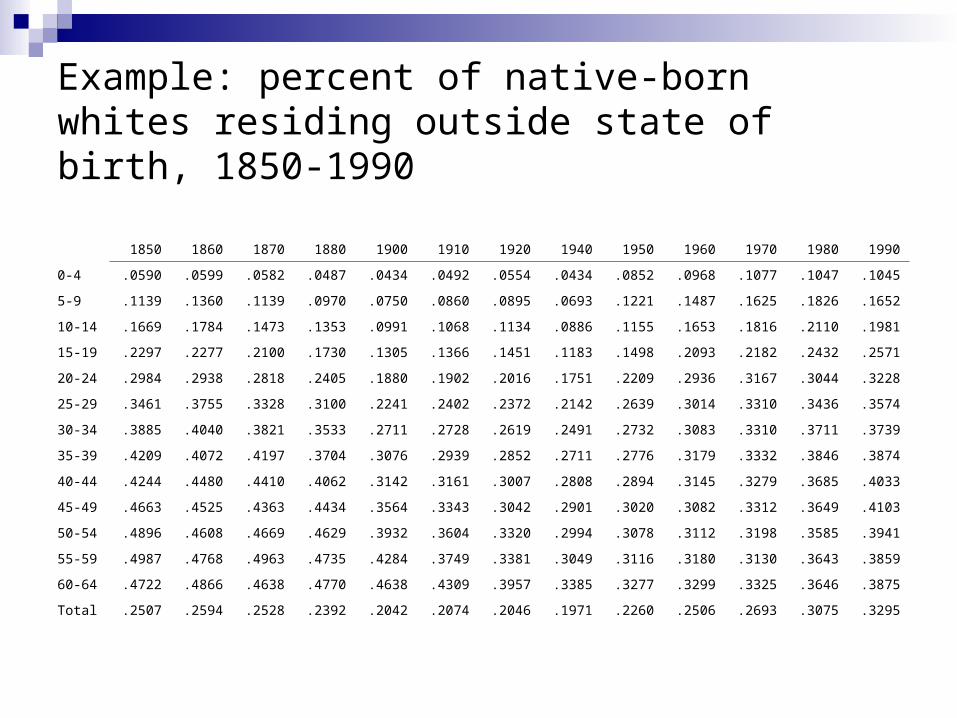
Example: percent of native-born whites residing outside state of birth, 1850-1990
1850 1860 1870 1880 1900 1910 1920 1940 1950 1960 1970 1980 1990
0-4 .0590 .0599 .0582 .0487 .0434 .0492 .0554 .0434 .0852 .0968 .1077 .1047 .1045
5-9 .1139 .1360 .1139 .0970 .0750 .0860 .0895 .0693 .1221 .1487 .1625 .1826 .1652
10-14 .1669 .1784 .1473 .1353 .0991 .1068 .1134 .0886 .1155 .1653 .1816 .2110 .1981
15-19 .2297 .2277 .2100 .1730 .1305 .1366 .1451 .1183 .1498 .2093 .2182 .2432 .2571
20-24 .2984 .2938 .2818 .2405 .1880 .1902 .2016 .1751 .2209 .2936 .3167 .3044 .3228
25-29 .3461 .3755 .3328 .3100 .2241 .2402 .2372 .2142 .2639 .3014 .3310 .3436 .3574
30-34 .3885 .4040 .3821 .3533 .2711 .2728 .2619 .2491 .2732 .3083 .3310 .3711 .3739
35-39 .4209 .4072 .4197 .3704 .3076 .2939 .2852 .2711 .2776 .3179 .3332 .3846 .3874
40-44 .4244 .4480 .4410 .4062 .3142 .3161 .3007 .2808 .2894 .3145 .3279 .3685 .4033
45-49 .4663 .4525 .4363 .4434 .3564 .3343 .3042 .2901 .3020 .3082 .3312 .3649 .4103
50-54 .4896 .4608 .4669 .4629 .3932 .3604 .3320 .2994 .3078 .3112 .3198 .3585 .3941
55-59 .4987 .4768 .4963 .4735 .4284 .3749 .3381 .3049 .3116 .3180 .3130 .3643 .3859
60-64 .4722 .4866 .4638 .4770 .4638 .4309 .3957 .3385 .3277 .3299 .3325 .3646 .3875
Total .2507 .2594 .2528 .2392 .2042 .2074 .2046 .1971 .2260 .2506 .2693 .3075 .3295

Highlight the same group over time
1850 1860 1870 1880 1900 1910 1920 1940 1950 1960 1970 1980 1990
0-4 .0590 .0599 .0582 .0487 .0434 .0492 .0554 .0434 .0852 .0968 .1077 .1047 .1045
5-9 .1139 .1360 .1139 .0970 .0750 .0860 .0895 .0693 .1221 .1487 .1625 .1826 .1652
10-14 .1669 .1784 .1473 .1353 .0991 .1068 .1134 .0886 .1155 .1653 .1816 .2110 .1981
15-19 .2297 .2277 .2100 .1730 .1305 .1366 .1451 .1183 .1498 .2093 .2182 .2432 .2571
20-24 .2984 .2938 .2818 .2405 .1880 .1902 .2016 .1751 .2209 .2936 .3167 .3044 .3228
25-29 .3461 .3755 .3328 .3100 .2241 .2402 .2372 .2142 .2639 .3014 .3310 .3436 .3574
30-34 .3885 .4040 .3821 .3533 .2711 .2728 .2619 .2491 .2732 .3083 .3310 .3711 .3739
35-39 .4209 .4072 .4197 .3704 .3076 .2939 .2852 .2711 .2776 .3179 .3332 .3846 .3874
40-44 .4244 .4480 .4410 .4062 .3142 .3161 .3007 .2808 .2894 .3145 .3279 .3685 .4033
45-49 .4663 .4525 .4363 .4434 .3564 .3343 .3042 .2901 .3020 .3082 .3312 .3649 .4103
50-54 .4896 .4608 .4669 .4629 .3932 .3604 .3320 .2994 .3078 .3112 .3198 .3585 .3941
55-59 .4987 .4768 .4963 .4735 .4284 .3749 .3381 .3049 .3116 .3180 .3130 .3643 .3859
60-64 .4722 .4866 .4638 .4770 .4638 .4309 .3957 .3385 .3277 .3299 .3325 .3646 .3875
Total .2507 .2594 .2528 .2392 .2042 .2074 .2046 .1971 .2260 .2506 .2693 .3075 .3295

Rearrange into birth cohorts
Year of birth
1846-1850 1896-1900 1936-1940
0-4 .0590 .0434 .0434
10-14 .1784 .1068 .1155
20-24 .2818 .2016 .2936
30-34 .3533 .3310
40-44 .2808 .3685
50-54 .3932 .3078 .3941
60-64 .4309 .3299

Make a nice graph
.0000
.0500
.1000
.1500
.2000
.2500
.3000
.3500
.4000
.4500
.5000
0-4 10-14 20-24 30-34 40-44 50-54 60-64
1846-18501896-19001936-1940

Synthetic cohorts
Similar to cohort analysis, but instead of using successive observations of the same group of people, you treat the age distribution of the population as if it were a cohort passing through time.
Yields different result from true cohort analysis in periods of rapid change
Synthetic cohorts are the basis of most commonly used measures of demographic behavior (e.g. life expectancy, total fertility rate, and median age at marriage.

Synthetic cohorts for internal migration
1850 1860 1870 1880 1900 1910 1920 1940 1950 1960 1970 1980 1990
0-4 .0590 .0599 .0582 .0487 .0434 .0492 .0554 .0434 .0852 .0968 .1077 .1047 .1045
5-9 .1139 .1360 .1139 .0970 .0750 .0860 .0895 .0693 .1221 .1487 .1625 .1826 .1652
10-14 .1669 .1784 .1473 .1353 .0991 .1068 .1134 .0886 .1155 .1653 .1816 .2110 .1981
15-19 .2297 .2277 .2100 .1730 .1305 .1366 .1451 .1183 .1498 .2093 .2182 .2432 .2571
20-24 .2984 .2938 .2818 .2405 .1880 .1902 .2016 .1751 .2209 .2936 .3167 .3044 .3228
25-29 .3461 .3755 .3328 .3100 .2241 .2402 .2372 .2142 .2639 .3014 .3310 .3436 .3574
30-34 .3885 .4040 .3821 .3533 .2711 .2728 .2619 .2491 .2732 .3083 .3310 .3711 .3739
35-39 .4209 .4072 .4197 .3704 .3076 .2939 .2852 .2711 .2776 .3179 .3332 .3846 .3874
40-44 .4244 .4480 .4410 .4062 .3142 .3161 .3007 .2808 .2894 .3145 .3279 .3685 .4033
45-49 .4663 .4525 .4363 .4434 .3564 .3343 .3042 .2901 .3020 .3082 .3312 .3649 .4103
50-54 .4896 .4608 .4669 .4629 .3932 .3604 .3320 .2994 .3078 .3112 .3198 .3585 .3941
55-59 .4987 .4768 .4963 .4735 .4284 .3749 .3381 .3049 .3116 .3180 .3130 .3643 .3859
60-64.4722 .4866 .4638 .4770 .4638 .4309 .3957 .3385 .3277 .3299 .3325 .3646 .3875
Total .2507 .2594 .2528 .2392 .2042 .2074 .2046 .1971 .2260 .2506 .2693 .3075 .3295

. . . And make a nice graph
.0000
.1000
.2000
.3000
.4000
.5000
.6000
0-4 5-9 10-14 15-19 20-24 25-29 30-34 35-39 40-44 45-49 50-54 55-59 60-64
1850
1880
1910
1940
1970
1990

Period change vs. cohort change vs. life course change
Period change refers to changes that occur from one year to the next
Cohort change is change occuring between successive birth cohorts
Often the two are different (example of fertility in the depression)
Life course change is change that occurs within a cohort as they age.

Period change: percent migrant among persons aged 55-59
.0000
.1000
.2000
.3000
.4000
.5000
.6000

Demographic synthetic cohort measures
Life expectancy: derives from life table; 2000 represents the number of years that would be lived by a synthetic cohort that experienced the same age-specific death rates as the population as a whole in 2000
Does not mean how long a baby born in 2000 can expect to live
There never has been and probably never will be a cohort that experiences the same age pattern of death
Cohort life tables are possible, but only for cohorts that are extinct.

Total fertility rate
Age-specific fertility rate is the number of births divided by the number of women at each age; or, the mean number of children born to women of each age in the course of a year (e.g., 2000).
Total fertility rate is the sum of the age-specific fertility rates over all ages
Total fertility represents the number of children that would be born to a hypothetical cohort that went through life experiencing the ASFRs of a particular period (assuming that none of them died before the end of their childbearing years)

Indirect Median age at first marriage
Another synthetic cohort measure Make a graph of percent ever-married in a census year,
and find the point at which half of those who will ever marry have married

Figure 1. Percent Ever Married by Age: White Women, 1970
0
10
20
30
40
50
60
70
80
90
100
Age
Per
cent
95% ever married
47.5% ever married
20.2 years
Calculation of median age at first marriage:
1) Percent ever-married = 95 %
2) Half of all women who will marry = 95/2 = 47.5%
3) Age at which 47.5% of women have married = 20.2 years
4) Add six months = 20.2 + .5 = 20.7 years

Other synthetic cohort measures
Years of schooling: from school attendance
Age at leaving home. But what if they come back?
Age at starting work, retiring, any transition that most people go through and usually do not return
Years with any characteristic

Years Lived Before Age 80 With Family and as Unrelated Individual, assuming no mortality: Synthetic cohorts in 1880, 1940, and 1950
Mean Years Lived Percent of Years Lived1900.0 1940.0 1950.0 1900.0 1940.0 1950.0
SingleWith family 24.9 26.5 24.3 31.1 33.1 30.4Unrelated 6.4 4.2 3.6 8.0 5.3 4.5Total Single 31.3 30.7 27.9 39.1 38.4 34.9
MarriedWith family 39.5 40.5 43.0 49.3 50.6 53.8Unrelated 1.5 1.4 1.1 1.9 1.8 1.4Total Married 41.0 41.9 44.1 51.3 52.4 55.1
Wid/DivWith family 4.6 3.5 3.3 5.8 4.4 4.1Unrelated 2.1 2.4 3.4 2.6 3.0 4.3Total Wid/Div 6.7 5.9 6.7 8.4 7.3 8.4
Institutional 1.0 1.5 1.2 1.3 1.9 1.5Total Years Lived 80.0 80.0 80.0 100.0 100.0 100.0

Same thing, adjusting for mortality
Mean Years Lived Percent of Years Lived1900 1940 1950 1900 1940 1950
SingleWith family 18.4 23.9 22.9 41.0 39.9 35.9Unrelated 4.0 3.0 2.8 8.8 5.0 4.4Total Single 22.4 26.9 25.7 49.8 44.9 40.3
MarriedWith family 19.1 28.1 32.6 42.4 46.9 51.1Unrelated 0.8 1.0 0.8 1.7 1.7 1.3Total Married 19.9 29.1 33.4 44.1 48.6 52.4
Wid/DivWith family 1.5 1.7 1.9 3.3 2.8 2.9Unrelated 0.8 1.2 2.0 1.8 2.0 3.2Total Wid/Div 2.3 2.9 3.9 5.1 4.8 6.1
Institutional 0.4 1.0 0.8 0.9 1.7 1.3Total Years Lived 45.0 59.9 63.8 100.0 100.0 100.0Total Years Dead 35.0 20.1 16.2 -- -- --