life-cycle assessment of urine diversion and conversion to
TRANSCRIPT

i
Life-Cycle Assessment of Urine Diversion and Conversion to Fertilizer Products
at the City Scale
by
Stephen Hilton
A thesis submitted
In partial fulfillment of the requirements
For the degree of Master of Science
(Environment and Sustainability)
In the University of Michigan
August 2020
Thesis Committee:
Professor- Gregory Keoleian, Chair
Professor Glen Daigger

ii
iii
ACKNOWLEDGMENTS
I would like to thank Dr. Greg Keoleian for his guidance, motivation, and for always
making time to help me. I appreciate him assisting me with this research, the degree, and the
steps after. I also appreciate Dr. Glen T. Daigger and Bowen Zhou for their guidance on
wastewater systems and many contributions throughout the project. I would like to thank Dr.
Nancy Love, Dr. William Tarpeh, the members of the UM Urine Diversion research project,
and the Rich Earth Institute for their expertise on urine diversion, their inspiring research,
and frequent support. I would also like to thank Dr. Steven Skerlos for his assistance with
earlier manuscripts, and Dr. Geoff Lewis for his frequent direction on Life Cycle Assessment
research methods. Lastly, I would like to thank the many people who supported me
throughout this project.
This research was supported by the U.S. National Science Foundation under award
number INFEWS 1639244 and the Water Research Foundation under project number STAR-
Na1R14/4899 to the University of Michigan.

iv
PREFACE
Separate collection of urine to recover nitrogen and phosphorus has been advocated to
enhance the sustainability of water management and food production. Urine could provide a
renewable source of nitrogen and phosphorus, which are currently extracted from nonrenewable
resources. Urine diversion also has the potential to prevent nutrients from entering water bodies
and to reduce the amount of energy and chemicals needed to treat wastewater. However, urine
diversion would require systems to collect urine, produce urine-derived fertilizers, and to ship
them, all of which have their own environmental impacts. This thesis explores the greenhouse
gas emissions, cumulative energy demand, freshwater use, eutrophication potential, and
acidification potential of systems that recover urine compared to those that do not. It evaluates
the importance of location-specific factors by focusing on three locations, and then by
conducting further sensitivity analysis. This work has been submitted to the journal
Environmental Science & Technology (currently in review).
v
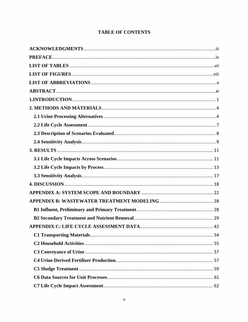
TABLE OF CONTENTS
ACKNOWLEDGMENTS ............................................................................................................ iii
PREFACE ...................................................................................................................................... iv
LIST OF TABLES ....................................................................................................................... vii
LIST OF FIGURES .................................................................................................................... viii
LIST OF ABBREVIATIONS ....................................................................................................... x
ABSTRACT ................................................................................................................................... xi
1.INTRODUCTION...................................................................................................................... 1
2. METHODS AND MATERIALS ............................................................................................. 4
2.1 Urine Processing Alternatives ............................................................................................ 4
2.2 Life Cycle Assessment ......................................................................................................... 7
2.3 Description of Scenarios Evaluated ................................................................................... 8
2.4 Sensitivity Analysis .............................................................................................................. 9
3. RESULTS ................................................................................................................................ 11
3.1 Life Cycle Impacts Across Scenarios ............................................................................... 11
3.2 Life Cycle Impacts by Process.......................................................................................... 13
3.3 Sensitivity Analysis ............................................................................................................ 17
4. DISCUSSION .......................................................................................................................... 18
APPENDIX A: SYSTEM SCOPE AND BOUNDARY ........................................................... 22
APPENDIX B: WASTEWATER TREATMENT MODELING ............................................ 28
B1 Influent, Preliminary and Primary Treatment ............................................................... 28
B2 Secondary Treatment and Nutrient Removal ................................................................. 29
APPENDIX C: LIFE CYCLE ASSESSMENT DATA............................................................ 42
C1 Transporting Materials ..................................................................................................... 54
C2 Household Activities .......................................................................................................... 55
C3 Conveyance of Urine ......................................................................................................... 57
C4 Urine Derived Fertilizer Production................................................................................ 57
C5 Sludge Treatment .............................................................................................................. 59
C6 Data Sources for Unit Processes....................................................................................... 61
C7 Life Cycle Impact Assessment .......................................................................................... 62

vi
APPENDIX D: SCENARIOS MODELED ............................................................................... 64
D1 Scenario Description ......................................................................................................... 64
D2 Electricity Production ....................................................................................................... 65
D3 Water Sources .................................................................................................................... 65
D4 Wastewater Treatment ..................................................................................................... 65
D5 Sludge Treatment and Disposal ....................................................................................... 67
D6 Transportation Distances.................................................................................................. 68
APPENDIX E: SENSITIVITY ANALYSIS ............................................................................. 70
APPENDIX F: SUPPLEMENTAL RESULTS ........................................................................ 75
F1 Comparison of Alternatives .............................................................................................. 75
F2 Impacts per Component .................................................................................................... 76
APPENDIX G: RESULTS OF THE SENSITIVITY ANALYSIS ......................................... 87

vii
LIST OF TABLES
Table 1. Important parameters to model urine collection and fertilizer production. ..................... 7
Table 2. Comparison of Three Scenarios. ...................................................................................... 9
Table 3. Life Cycle Impacts per Scenario .................................................................................... 11
Table 4. Primary Influent per Capita. .......................................................................................... 28
Table 5. Primary Removal Efficiencies. ...................................................................................... 29
Table 6. Wastewater Conversion Factors. ................................................................................... 30
Table 7. Parameters used to model metabolic activity. ............................................................... 30
Table 8. Parameters used to model metabolic activity. ............................................................... 31
Table 9. Pumping head in secondary treatment. .......................................................................... 38
Table 10. List of inputs used to model the life cycle assessment. ............................................... 42
Table 11. Description of flush volumes. ...................................................................................... 56
Table 12. List of data sources used to quantify environmental impacts. ..................................... 61
Table 13. Environmental impacts of electricity production. ........................................................ 65
Table 14. Sources of Potable Water by Location. ....................................................................... 65
Table 15. Effluent Wastewater Standard for input in Each Location. ......................................... 66
Table 16. Description of WWTPs in Michigan. .......................................................................... 67
Table 17. Sludge Treatment Methods used in each Scenario. ..................................................... 68
Table 18. End of life for biosolids in each scenario. ................................................................... 68
Table 19. Shipping distances in different scenarios..................................................................... 69
Table 20. List of distributions for parameters in the Monte Carlo analysis. ............................... 71
Table 21. Urine Concentration Scenarios with lower GWP. ....................................................... 90
Table 22. Struvite and Ammonium Sulfate Scenarios with lower GWP. .................................... 90

viii
LIST OF FIGURES
Figure 1 a-c. System Diagram for each alternative. ....................................................................... 5
Figure 2. Normalized impacts in Virginia Scenario. ................................................................... 12
Figure 3. GWP by Process. .......................................................................................................... 14
Figure 4. Reductions in GHGs in WWTPs. ................................................................................. 16
Figure 5. Detailed description of Study Scope. ........................................................................... 23
Figure 6. Depiction of simulations ran in sensitivity analysis. .................................................... 70
Figure 7. Normalized Impacts in Vermont Scenario. .................................................................. 75
Figure 8. Normalized Impacts in Michigan Scenario. ................................................................. 76
Figure 9. GWP of the Vermont alternatives by Process. ............................................................. 76
Figure 10. CED of the Vermont alternatives by Process. ............................................................ 77
Figure 11. Freshwater use of the Vermont alternatives by Process. ............................................ 77
Figure 12. Eutrophication potential of the Vermont alternatives by Process. ............................. 78
Figure 13. Acidification potential of the Vermont alternatives by Process. ................................ 78
Figure 14. GWP of the Michigan alternatives by Process. .......................................................... 79
Figure 15. CED of the Michigan alternatives by Process. ........................................................... 79
Figure 16. Freshwater use of the Michigan alternatives by Process. ........................................... 80
Figure 17. Eutrophication potential of the Michigan alternatives by Process. ............................ 81
Figure 18. Acidification potential of the Virginia alternatives by Process. ................................. 82
Figure 19. CED of the Virginia alternatives by Process. ............................................................. 82
Figure 20. Freshwater use of the Virginia alternatives by Process. ............................................. 83
Figure 21. Eutrophication potential of the Virginia alternatives by Process. .............................. 83
Figure 22. Acidification potential of the Virginia alternatives by Process. ................................. 84
Figure 23. Comparison of WWTP Modeling Methods. .............................................................. 84
Figure 24. Differences in GHGs from Urine Concentration in sensitivity analysis. ................... 87
Figure 25. Differences in GHGs from Struvite and Ammonium Sulfate in sensitivity analysis. 87
Figure 26. Differences in APs from Urine Concentration in sensitivity analysis. ....................... 88
Figure 27. Differences in APs from Struvite and Ammonium Sulfate in sensitivity analysis. ... 88
Figure 28. GWP Comparison of Urine Concentration and Struvite and Ammonium Sulfate in
5SB. ............................................................................................................................................... 89
Figure 29. GWP Comparison of Urine Concentration and Struvite and Ammonium Sulfate in
SAB. .............................................................................................................................................. 89

ix
x
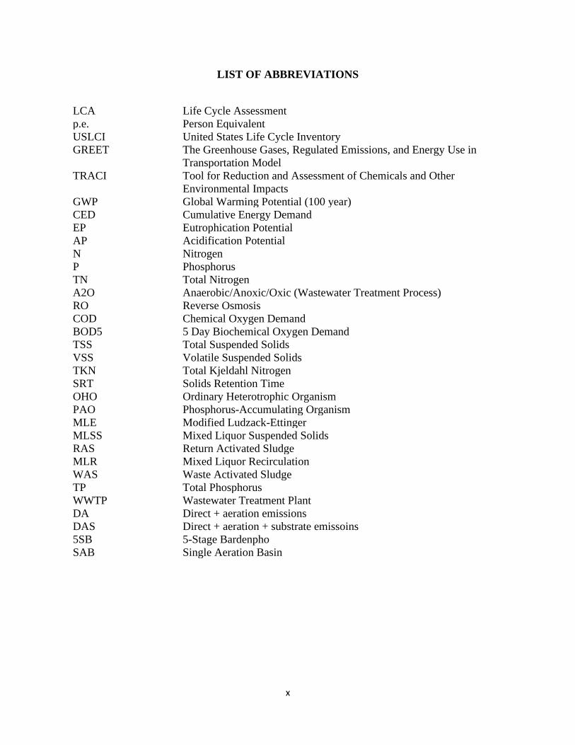
LIST OF ABBREVIATIONS
LCA Life Cycle Assessment
p.e. Person Equivalent
USLCI United States Life Cycle Inventory
GREET The Greenhouse Gases, Regulated Emissions, and Energy Use in
Transportation Model
TRACI Tool for Reduction and Assessment of Chemicals and Other
Environmental Impacts
GWP Global Warming Potential (100 year)
CED Cumulative Energy Demand
EP Eutrophication Potential
AP Acidification Potential
N Nitrogen
P Phosphorus
TN Total Nitrogen
A2O Anaerobic/Anoxic/Oxic (Wastewater Treatment Process)
RO Reverse Osmosis
COD Chemical Oxygen Demand
BOD5 5 Day Biochemical Oxygen Demand
TSS Total Suspended Solids
VSS Volatile Suspended Solids
TKN Total Kjeldahl Nitrogen
SRT Solids Retention Time
OHO Ordinary Heterotrophic Organism
PAO Phosphorus-Accumulating Organism
MLE Modified Ludzack-Ettinger
MLSS Mixed Liquor Suspended Solids
RAS Return Activated Sludge
MLR Mixed Liquor Recirculation
WAS Waste Activated Sludge
TP Total Phosphorus
WWTP Wastewater Treatment Plant
DA Direct + aeration emissions
DAS Direct + aeration + substrate emissoins
5SB 5-Stage Bardenpho
SAB Single Aeration Basin

xi
ABSTRACT
Urine diversion has been proposed as an approach for producing renewable fertilizers and
reducing nutrient loads to wastewater treatment plants. Life cycle assessment was used to
compare environmental impacts of the operations phase of urine diversion and fertilizer
processing systems (via 1) a urine concentration alternative and 2) a struvite precipitation and ion
exchange alternative) at a city scale to conventional systems. Scenarios in Vermont, Michigan,
and Virginia were modeled, along with additional sensitivity analysis to understand the
importance of key parameters, such as the electricity grid and wastewater treatment method.
Both urine diversion technologies had better environmental performance than the conventional
system, and led to reductions of 29-47% in greenhouse gas emissions, 26-41% in energy
consumption, approximately half the freshwater consumption, and 25-64% in eutrophication,
while acidification ranged between a 24% decrease to a 90% increase. In some situations
wastewater treatment chemical requirements were eliminated. The environmental performance
improvement was usually dependent on offsetting the production of synthetic fertilizers. This
study suggests that urine diversion could be applied broadly as a strategy for both improving
wastewater management and decarbonization.
1
INTRODUCTION
About half of the world food supply depends on synthetic fertilizers produced from
nonrenewable resources 1.Phosphate rock is used to produce phosphorus fertilizers. While the
extent of the resource base is contested, supply is finite, demand has increased partly due to
increased meat consumption and biofuel production, and supplies are dominated by a few
countries. 2–5 Production of nitrogen fertilizer depends on natural gas, and is responsible for
about 1.2% of world energy use and associated greenhouse gas emissions. 6,7 Prices for
phosphate rock and other fertilizer commodities have fluctuated as much as 800% in recent
years, which has led to food riots in many countries.3,4,8 Given the impacts and resource
constraints of conventional fertilizers, renewable and reliable alternatives are needed.
Food consumption by humans is the principal source of these vital nutrients in domestic
wastewater, and significant resources are invested to remove them to protect the aquatic
environment. Water and wastewater systems consume about 3-4% of the total electricity in the
United States, with nutrient removal often being one of the most energy intensive processes.9,10
Some propose separately collecting urine and using it to produce fertilizer.11,12 Although it
comprises less than 1% of wastewater volume, urine contains approximately 50% of the
phosphorus and 80% of the nitrogen contained in domestic wastewater. 13–15 As utilities
increasingly focus on sustainability, large-scale urine diversion has the potential to improve
regional wastewater management, recover essential resources and reduce energy consumed in
processes such as aeration. 11,16–19

2
Compared to synthetic fertilizers, urine-derived fertilizers recover important nutrients,
can be as effective at stimulating plant growth, and contain lower levels of heavy metals. 19–26
However, processing fertilizers from urine will have environmental impacts. 15 Collecting and
transporting urine will require new infrastructure systems, such as pressurized pipe networks or
truck collection.
Use of acetic acid or other chemicals may be needed to prevent the spontaneous release
of ammonia gas and formation of precipitates that clog piping infrastructure. 15,27–29 Urine
concentration, through processes such as reverse osmosis, freeze thaw, or distillation, may be
required to make nutrient concentrations in urine, which are much lower than synthetic fertilizer,
high enough for efficient agricultural application. 15,30–34 Alternatively, nutrients may be
concentrated through removal processes such as struvite precipitation, ammonia capture via ion
exchange, or urea adsorption. 15,20,35–41 Additional treatment to deactivate pathogens and remove
pharmaceuticals found in urine may also be needed.
Life Cycle Assessment (LCA) is well suited to compare the environmental performance
of urine diverting systems to conventional systems, determine environmental hotspots, and
highlight trade-offs and opportunities for system improvement.42,43 LCA has been used to
compare a range of wastewater treatment alternatives, 44–47 and in most cases has indicated that
urine diversion has lower environmental impacts than conventional systems . 13,14,48–51 However,
these studies have focused on small scale systems, have evaluated only a few locations and
urine-derived fertilizers, and simplified how diverting urine will affect wastewater treatment
plants. These studies measure changes to wastewater through volume reduction or a static offset
for denitrification, which may not capture significant changes to wastewater treatment as nutrient
ratios change, or how urine diversion could change treatment configurations.48,49,52–54
3
This study expands upon previous research by evaluating the environmental impacts of
urine diversion and conversion to fertilizer relative to conventional alternatives in large and
diverse settings, and by a more detailed assessment of how this will affect wastewater treatment.
This conventional alternative manages urine through the wastewater system and produces and
transports equivalent amounts of nutrients in the form of synthetic fertilizer. The relative
differences between these two different approaches are quantified. Wastewater treatment is
modeled in detail to better account for the ramifications of urine diversion. Three distinct
locations, namely the States of Vermont, Michigan, and Virginia (referred to subsequently as
scenarios) are considered to explore how important parameters such as population, extent of
nutrient removal at wastewater treatment plants, electricity grid fuel mix and the amount of
urine-derived fertilizer produced influence the environmental performance. Sensitivity analysis is
conducted using Monte Carlo in order to further evaluate these parameters and the uncertainty of
many others.

4
2. METHODS AND MATERIALS
2.1 Urine Processing Alternatives
Two distinct urine-derived fertilizer alternatives were evaluated to represent the range of
products that can be produced. They consist of (1) concentrated urine, where organics such as
pharmaceuticals are removed from diverted urine through activated carbon and urine is
subsequently concentrated by reverse osmosis (RO) and then heat pasteurized, and (2) struvite
and ammonium sulfate, where urine is processed to produce struvite through precipitation and
ammonium sulfate through ion exchange. Use of urine-derived fertilizer products are compared
to commercial fertilizers. For the urine-derived fertilizer alternatives it was assumed that 70
percent of urine in each of the three scenarios considered was diverted for fertilizer production.
This was done to simulate large-scale collection within these locations but to allow for some
inefficiency in collection. As shown in Figure 1, production and distribution of flushwater,
collection of wastewater (including separated urine), production and transportation of fertilizers,
and wastewater treatment were included in the scope of the study to capture system-wide
differences.

5
Figure 1 a-c. System Diagram for each alternative.
a) The urine concentration alternative, b) the struvite and ammonium sulfate alternative, c) the
conventional system. Yellow boxes indicate that a process is either unique to that alternative, or
that urine diversion significantly affects its environmental impact.
The inputs to treat and distribute flush water were determined using the ratio of surface
and groundwater treated in each location,55 and literature data for both types of treatment. 48,56,65–
67,57–64 When urine was diverted, urine diversion toilet flush volumes were used. In the
conventional alternative, for people not using urine-diverting toilets, and during defecation, low-
flow toilet flush volumes were used, as shown in Tables 11 & 12. When urine is diverted, acetic
acid is added to stabilize it, followed by transportation to a fertilizer production center via a
pressurized pipe system.
Magnesium oxide is added to precipitate phosphorus as struvite and the remaining
ammonium from the effluent is captured through ion exchange using a resin such as Dowex Mac

6
3.39 The exhausted resin is regenerated with 3 M sulfuric acid, producing a liquid ammonium
sulfate fertilizer. Additional acetic acid is needed for the concentrated urine fertilizer to
consistently maintain nitrogen in the urea form. Following pharmaceutical removal using
activated carbon, urine is concentrated to a fifth of its original volume using reverse osmosis
with an energy recovery device (ERD) and then heat pasteurized. Chemical and energy inputs for
regeneration of activated carbon68–72 and reverse osmosis membrane cleanings73 are included.
Effluents from the urine-derived fertilizer production facilities are sent to the wastewater
treatment plant, and the urine-derived fertilizers are trucked to a regional fertilizer distributor.
The methodology described in Hilton et al.74 is used to model wastewater treatment for
all alternatives to determine electricity consumption, chemical consumption, secondary sludge
production, water and air emissions. All alternatives assumed equal amounts of feces and
greywater, steady state conditions, and compliance with all regulatory requirements. Processes
that were equivalent in magnitude between alternatives, such as primary sludge treatment and
hauling screenings to landfills, were excluded. Further details can be found in the supplemental
materials, Figure S1, and Hilton et al.74
The production of urea and mono-ammonium phosphate fertilizers and transportation to
the regional fertilizer distribution center was used to ensure all alternatives provided the same
mass of nitrogen and phosphorus as fertilizer. These synthetic fertilizers were added in the
conventional and both diversion alternatives to provide equal amounts of nitrogen and
phosphorus despite differing nutrient recovery ratios. Transportation from the regional fertilizer
distribution center and application at the farm were not analyzed, as previous research did not
find plant uptake and runoff from urine-derived fertilizers to differ from synthetic fertilizers.25,75–
77
7
2.2 Life Cycle Assessment
The treatment of one person equivalent’s (p.e.) wastewater for one year is the functional
unit of analysis used. Treatment of all wastewater produced (including urine as appropriate) is
considered because urine diversion can lead to significant reductions in the nitrogen and
phosphorus of wastewater arriving at the treatment plant, and can significantly affect treatment.
All alternatives provided equal masses of nitrogen and phosphorus in fertilizer. Environmental
burdens of capital equipment and the end of life of wastewater and fertilizer infrastructure were
excluded because the operational phase impacts are expected to dominate. 78–81
Parameters used for the life cycle inventory and mass balance were obtained from
literature sources and pilot scale systems, and can be found in Tables 1, 11 and 13. The United
States Life Cycle Inventory (USLCI) was used for most unit processes, though Ecoinvent was
used when unit processes were not available.82,83 A Life Cycle Impact Assessment was
conducted using global warming potential (GWP), cumulative energy demand (CED), freshwater
use,84 eutrophication potential (EP), and acidification potential (AP). These categories represent
key impacts for changes in energy use, chemical manufacturing, water quality, and water use that
are caused by urine diversion.
Table 1. Important parameters to model urine collection and fertilizer production.
Process Parameter Value Unit Notes and
Sources
Home/Collection
Flushes per
person per
day
3.8,5.14 /pe۰day Urine only,
then total.85–90
Conventional:
water per
flush
4.84 L/flush
Also used for
feces flushes in
UD toilets

8
Urine
diversion:
water per
flush
0.165 L/flush
Used for urine-
only flushes.
Personal
conversation
Raye-Leonard 18
5% acetic
acid added
0.033-
0.04
L/L urine
and
flushwater
Struvite and
ammonium
sulfate
(Calculated)
then Urine
Concentration
(Experimentally
determined 25)
Struvite and
Ammonium
Sulfate
Production
Mg:P ratio
for struvite 1.5:1 48,54,91,92
Sulfuric acid
per kg N 16.7 liters/kg N
18%. Tarpeh,
personal
conversation.
N and P
recovery 96, 96 % 39,48,54,93,94
Concentrated
Urine
Production
RO electricity
consumption 0.009
kWh/l
removed
Noe-Hays,
Personal
Communication
N & P
Recovery 95, 99 % 95,96
2.3 Description of Scenarios Evaluated
Three scenarios were modeled to provide an initial assessment of how location-specific
factors affect the environmental merits and drawbacks of urine diversion. The Vermont scenario

9
represents a smaller urban community without strict nitrogen effluent limits located in a largely
rural state. The Michigan scenario was developed as a statewide average and was constructed by
categorizing the range of communities in the State, the types of wastewater treatment plants
found, and wastewater treatment volumes. The Virginia scenario represents a more densely-
populated urban location with strict effluent limits. Further description of these scenarios can be
found in the supplemental materials, Tables 2 and 14-20, and Hilton et al. 74 All alternatives were
evaluated for each scenario.
Table 2. Comparison of Three Scenarios.
Item Vermont Michigan Virginia
Description Largely rural state
with small to mid-
size communities
Large state with
diverse range of
community sizes
Stringent effluent
discharge standards
Population Modeled 25,000 150,000 350,000
Effluent Discharge
Standards
Secondary, P limits Secondary, P, some
ammonia and TN
limits
Advanced Secondary,
stringent TN and P
limits
Wastewater
Treatment
Process(es)
Single Aeration Basin Single Aeration
Basin, Nitrification,
A2O
5-Stage Bardenpho
Typical Distance to
Fertilizer Distributors
50 50 41
GWP of Electricity
(kg CO2e/kWh)
0.107 0.544 0.450
2.4 Sensitivity Analysis
Sensitivity analysis was conducted to evaluate the robustness of the results, test urine
diversion in a broader range of contexts, and to elucidate how model parameters and key
assumptions influenced the environmental performance of urine diversion. Twelve separate
simulation scenarios were created. As shown in Figure S2, six of these simulation scenarios
modeled the 5-Stage Bardenpho treatment plant because it had the highest level of nutrient

10
removal, while six modeled the single aeration basin with phosphorus removal because it had the
lowest level of nutrient removal. Three electric grids, coal, natural gas, and renewable comprised
of 50% wind and 50% hydropower were considered for each wastewater treatment type. Both the
urine concentration, and struvite and ammonium sulfate urine derived fertilizer alternatives were
compared, given six simulations for each wastewater treatment type. Table 21 lists the
distributions of each parameter used. The Excel plugin Simvoi was used to conduct a Monte
Carlo analysis with 10,000 repetitions for each sensitivity scenario97.

11
3. RESULTS
3.1 Life Cycle Impacts Across Scenarios
Urine diversion consistently provides improved environmental performance relative to the
conventional system for each scenario for all impact categories, except AP, as shown in Table 3.
Both diversion alternatives reduced the GWP, CED, freshwater use, and EP categories from
anywhere between 26% to 64%. The urine concentration alternative typically led to larger
improvements than the struvite and ammonium sulfate alternative. Urine concentration
alternatives decreased the AP modestly compared to the conventional alternative for all scenarios
(12-24%), while struvite and ammonium sulfate alternatives increased the AP by 34% to 91%
relative to the conventional alternative. Figures 2, 7, and 8 provide the relative differences in
environmental performance for each alternative.
Table 3. Life Cycle Impacts per Scenario
Scenario Alternative GWP CED Freshwater
Use
Eutrophication
Potential
Acidification
Potential
kg
CO2e
MJ m3 kg N eq kg SOx eq
Vermont Urine
Concentration
14.6 297 7.28 1.19 0.0510
Struvite and
Ammonium
Sulfate
19.7 313 7.37 1.27 0.111
Conventional 27.6 450 13.7 3.27 0.0581
Michigan Urine
Concentration
30.1 441 7.66 1.44 0.123
Struvite and
Ammonium
Sulfate
33.5 456 7.78 1.51 0.180
Conventional 47.9 616 15.1 3.58 0.135

12
Virginia Urine
Concentration
22.9 376 6.67 0.295 0.0728
Struvite and
Ammonium
Sulfate
26.1 382 6.73 0.302 0.130
Conventional 36.8 637 12.8 0.405 0.0941
Figure 2. Normalized impacts in Virginia Scenario.
Total impacts in each alternative normalized to the maximum value in each category.
The magnitude of environmental impacts differed substantially between the three
scenarios. Michigan had the highest GWP, CED, and AP impacts, while Vermont had the lowest.
Much of this is because Michigan’s electricity grid is comprised primarily of fossil fuels and
uses natural gas to thermally dry sludge, while Vermont’s electricity grid is mostly comprised of
renewable energy sources. The Vermont scenario had an EP approximately four times larger than
in Virginia as a result of the large differences in effluent standards. The urine diversion
alternatives in states with less stringent effluent standards (Vermont and Michigan) saw the
0%
10%
20%
30%
40%
50%
60%
70%
80%
90%
100%
GWP CED Water EP AP
Per
cen
t o
f M
axim
um
Impact Category
Urine Concentration Struvite and Ammonium Sulfate Conventional

13
largest decreases in EP. The differences between the urine concentration, and struvite and
ammonium sulfate alternatives were smaller for scenarios where the environmental impacts of
producing electricity were larger, such as in Michigan.
3.2 Life Cycle Impacts by Process
Figure 3 shows the contribution of system components to greenhouse gas emissions for
the Virginia scenario (see Figures S5-S18 for all impact categories and scenarios). Wastewater
treatment dominated the eutrophication potential (81-99%), was usually responsible for the
largest proportion of impacts in GWP (46-56%) and CED (35-49%) categories, and was a major
contributor to AP (16-64%). Fertilizer production had the next largest impacts in the GWP (15-
38%), CED (17-30%), and EP (0-17%) categories, and was a major contributor to AP (9-63%).
In Michigan and Vermont, the EP from fertilizer production was negligible relative to its
contribution from wastewater effluent. Potable water production and urine collection
respectively had the next largest impacts in the GWP and CED categories. The largest
contributor to AP was sulfuric acid (36%-58% when producing ammonium sulfate) followed by
acetic acid (11-17% when producing ammonium sulfate, 20%-48% when concentrating urine).

14
Figure 3. GWP by Process.
Global warming potential of the Virginia alternatives broken down by process.
In the conventional alternative, 10.4 cubic meters of water were needed per person per
year for flushing excluding leaks between the drinking water plant and the consumer. This
decreases to 5.3 and 3.1 cubic meters for 70% and 100% urine diversion, respectively. Reduced
flush volumes from urine-diverting toilets were responsible for the majority of decreased
freshwater used although 9 to 11% came from upstream sources such as production of synthetic
fertilizer, ferric chloride, and other chemicals.
For urine collection, producing acetic acid led to higher environmental impacts than the
electricity consumed to collect urine. More acetic acid was used to ensure that urine remained
stable in the urine concentration alternative. While urine diversion reduced the volume of
wastewater that needed to be collected, the impacts of collecting and stabilizing urine were
substantially larger than any benefits of collecting less wastewater in sewers.
0
5
10
15
20
25
30
35
40
Urine Concentration Struvite and AmmoniumSulfate
Conventional
kg C
O2e
/ca
pit
a۰ye
ar
VirginiaGlobal Warming Potential
Others Synthetic fertilizerTransport UDF Production-ChemicalsUDF Production-Electricity Urine CollectionSecondary Sludge Treatment Wastewater Treatment (excluding sludge)Water Production
15
Urine-derived fertilizer production resulted in about 21-75% as much GWP as synthetic
fertilizers and decreased most other environmental impacts. The exception was AP, which
ranged anywhere from a 77% decrease to a 231% increase from synthetic fertilizers. Offsetting
synthetic fertilizers was almost always required to reduce GWP and CED.
The impacts of concentrating urine were dominated by electricity consumed for reverse
osmosis. Unless urine diversion led to major reductions in electricity consumed at wastewater
treatment plants, such as in Virginia, concentration increased total electricity within a
municipality. The environmental impacts of producing concentrated urine were low in Vermont
due to the high proportion of renewable energy. The impacts of producing struvite and
ammonium sulfate were relatively consistent, with sulfuric acid being responsible for much of
the GWP and leading to this alternative always having the largest AP. Processes such as
regenerating activated carbon, cleaning RO membranes, producing magnesium oxide and ion
exchange resin, and electricity for pumping in the fertilizer production facility had small overall
impacts.
The GWP and CED of shipping urine-derived fertilizers to the fertilizer depot comprised
a relatively small portion of the net impact, but were up to 3.5 times higher than shipping
synthetic fertilizers. Synthetic fertilizers were shipped much longer distances, but only required
about 4-8% as much mass, and were more likely to use larger and more efficient transports.
Urine diversion significantly decreased the impacts (GWP, CED, AP) of nutrient removal
from treatment plants with stringent effluent limits, whereas more lenient plants reduced the EP
of releasing effluent to aquatic ecosystems. As shown in Figure 4, all treatment plants benefitted
by reducing the amount of ferric chloride required to remove phosphorus. Treatment plants with
stricter effluent limits had larger reductions of electricity, methanol, and nitrous oxide emissions

16
in biological treatment. These benefits were so large in Virginia that even if no synthetic
fertilizer were offset, urine diversion would still reduce net greenhouse gas emissions. In certain
cases, urine diversion could eliminate the need for ferric chloride and methanol during average
conditions. Reducing total wastewater volume, capturing BOD in concentrated urine, and minor
changes to secondary sludge production led to small changes in environmental impacts.
Figure 4. Reductions in GHGs in WWTPs.
Reductions in greenhouse gas emissions from different types of wastewater treatment plants due
to 70% urine diversion. All remove phosphorus and use the Virginia electricity grid to allow
comparison. The first type has an aeration basin to remove BOD (Vermont). The second
category uses nitrification to oxidize ammonia to nitrate. The third category further treats
wastewater with denitrification, which converts some nitrate to nitrogen gas. The final category
is the 5-Stage Bardenpho treatment method which removes the most nutrients (Virginia).
Figure 23 shows that the methodology used in this study and the simpler methodologies
used in other studies to estimate how much urine diversion reduces greenhouse gas emissions
from wastewater treatment are within a reasonable range.48,49 However, the benefits from
increasing urine are not linear due to elimination of chemical requirements or changes in
wastewater treatment plant configuration, so the use of an linear offset results in some level of
inaccuracy.
0
1
2
3
4
5
6
7
8
9
10
No NitrogenRemoval
Nitrification Nitrification andDenitrification
5-Stage Bardenpho
GP
W (
kg C
O2e
/per
son
·yea
r)
Methanol Lime Ferric Chloride Nitrous Oxide Electricity in Secondary

17
3.3 Sensitivity Analysis
Figures 24-27 demonstrate that the results of this study were largely robust. Urine
diversion always decreased freshwater use and EP. The number of repetitions where urine
concentration increased GWP and CED were negligible, but occurred occasionally for struvite
and ammonium sulfate when renewable electricity was used. Urine concentration alternatives did
increase AP in a few repetitions with the Five-Stage Bardenpho when renewable electricity was
used, and approximately 30% of repetitions in the single aeration basin. The AP for struvite and
ammonium sulfate was always higher than the conventional alternative even as the efficiency of
ammonium sulfate use approached 100%. Figures 28 and 29 show that urine concentration
typically had a better environmental performance than struvite and ammonium sulfate. These
differences were more pronounced when producing electricity had lower environmental impacts
because the added burden of electricity consumption to concentrate urine was lessened.
Environmental improvements in GWP, CED, and AP categories are highest in locations with
electricity produced from fossil fuels and large levels of nutrient removal, as shown in Figures
24-27. Environmental improvements are also greater in locations with less wastewater volume
per person and lower performing aeration systems.
Tables 22 and 23 show that excluding fertilizer offsets and nitrous oxide emissions from
effluents from the scope can change the conclusion of the analysis. As the environmental impact
of producing electricity decreased, reducing greenhouse gases without considering fertilizer is
less likely. The exception is for urine concentration alternatives with limited nutrient removal
because net electricity consumption in a municipality increases. When nitrous oxide emissions
from effluent were not considered, urine diversion almost never decreased greenhouse gas
emissions from single aeration basin systems that use renewable electricity.

18
4. DISCUSSION
Similar to other life cycle assessments,48,49,51 this study found urine diversion reduced
most environmental impacts. It expanded upon previous research by conducting a more
comprehensive characterization of wastewater treatment and by evaluating a range of large-scale
systems. Simpler methods to estimate the changes in environmental impacts of treating
wastewater are valid as an approximation, but the more complete methods used in this study may
be more appropriate when increased accuracy is needed or when different extents of urine
diversion are being evaluated. Scenario and sensitivity analyses showed that freshwater use and
EP impacts were always reduced, GWP and CED were consistently reduced, and urine
concentration usually reduced the AP.
Urine collection is the uncertain aspect of this analysis due to a lack of large-scale
examples. This study modeled a centralized system conveying urine from an urban area to a
central processing facility in order to create a reasonable estimate of the environmental burdens
from urine collection. It suggested the importance of the acetic acid dosage used for stabilization.
Other options include a more distributed system consisting of multiple processing facilities
strategically located throughout an urban area to reduce both the distance collected urine would
need to be transported, as well as the transport time which could reduce urine stabilization
requirements. The optimal scale of decentralization of urine collection still needs to be assessed.
Significant further development of urine collection is certainly possible which could reduce not
only cost but environmental impacts.
The advantages urine diversion provides wastewater treatment are clearly demonstrated
in this study and corroborated by previous research.18,52 Where nutrient removal is practiced,

19
these primarily include elimination of chemical inputs (metal salts for phosphorus removal,
supplemental carbon such as methanol for nitrogen removal) and reduced energy use. In many
cases urine diversion can eliminate the need to expand existing wastewater treatment plants for
nutrient removal capabilities. While not considered in this study, eliminating the need for
nutrient removal could allow further changes to treatment process such as increased capture and
utilization of organic matter contained in the influent wastewater. In locations where nutrient
removal is not a goal for wastewater treatment, eutrophication can be reduced as less nutrients
are discharged to local waterways. Urine diversion leads to decreases in environmental impacts
through a wide range of conditions, but can be a particularly effective decarbonization strategy in
areas with high levels of nutrient removal, electricity produced primarily from fossil fuels, and
relatively little wastewater per capita.
Producing fertilizer from urine instead of mineral sources leads to significant
environmental benefits. These urine-derived fertilizer production methods were characterized
using laboratory and demonstration scale-studies, 25,26,37–39,54,98 but demonstration of other
available approaches15,33,40,41,92 and larger scale systems will provide an improved basis for
assessing environmental impacts.15,33,40,41,92 They were selected to represent a range of fertilizer
products and production methods. Urine concentration is more heavily dependent on energy,
produces a fertilizer with nitrogen in the form of urea, retains much of the potassium in urine,
and has a relatively consistent nitrogen-to-phosphorus ratio (depending on the composition of
urine and whether additional nutrients are added). Struvite precipitation and ammonium sulfate
largely use chemical inputs and could easily be applied with different nitrogen-to-phosphorus
ratios. Throughout all electricity grids, the environmental burdens of producing concentrated
urine were usually lower even as the efficiency of sulfuric acid use approached 100%. A
20
comprehensive environmental evaluation of all the different forms of urine derived fertilizers is
needed for a complete life-cycle perspective. The environmental burdens of producing them
were lower than synthetic fertilizers, and will be significantly improved as use of sulfuric acid
for ion exchange and energy for reverse osmosis are optimized, or renewable energy is used for
urine concentration.
The urine-derived fertilizers evaluated could be applied similarly to fertilizers commonly
used in the US.99 Beyond the impacts of fertilizer production, other important factors such as the
higher popularity of single-nutrient fertilizers will affect which fertilizers are produced.99
Implementation efforts need to consider the fertilizer demands of adjacent communities and the
transportation costs and environmental impacts associated with shipping urine-derived fertilizers
from population centers.12,100
Urine can replace a significant fraction of synthetic fertilizers. Researchers estimate 16-
30 kilograms of nitrogen and 4 kg of phosphorus in fertilizer are currently used per person per
year in affluent countries.101–104 If all nutrients were recovered from domestic wastewater it
would likely produce less than 5 kg of nitrogen and 1 kg of phosphorus per person. Regardless,
urine diversion can provide significant environmental benefits and can be used with other
strategies such as dietary changes, manure application, and reduction of nutrient runoff during
mineral extraction and fertilizer application to significantly improve nutrient use efficiency.101,102
The development of large-scale urine collection and processing systems is still at a
conceptual stage. Research is ongoing to understand and address the many challenges of urine
diversion, including economic, market and regulatory acceptance,12,26,105–108 potential user
error,26,109 risk aversion and lack of confidence in performance,8,106,107 and lock-in to
conventional systems.107,110 Irrespective of the urine processing method considered, net benefits
21
were observed for each scenario evaluated. In some cases the environmental benefits associated
with water and wastewater management alone were sufficient to offset the environmental burden
associated with urine collection, processing, and transport. The analyses presented here clearly
indicate that the more well-defined benefits (reduced wastewater management requirements and
avoided synthetic fertilizer production) exceed the environmental impacts of urine collection,
processing, and transport, suggesting that further efforts to develop such systems are warranted.
22
APPENDIX A: SYSTEM SCOPE AND BOUNDARY
This section will provide a more in-depth description of what is and is not included in the
scope of this study. This study only considers the use phase, so burdens from infrastructure and
decommissioning are excluded. There are important exclusions from the use phase, so the
impacts should not be interpreted as the total impact of the urban water system.
In order to conduct this Life Cycle Assessment (LCA), mass balances were tracked
through much of the urban water cycle. The environmental impacts of managing some of these
flows were quantified. While this study evaluates certain environmental burdens of processes
that remove pharmaceuticals from urine, a mass balance on pharmaceuticals was not conducted.
The impacts from releasing pharmaceuticals into aquatic or terrestrial ecosystems were not
considered.
Relevant material flows fall into four general categories:
1. Mass, volume, and environmental impacts are considered.
2. Only the mass and volume are considered.
a. For example, considering other wastewater flows (e.g. stormwater) to estimate
wastewater dilution.
3. Mass, volume, and environmental impacts are excluded from consideration due to
similarity between alternatives.
a. For example, primary sludge was not tracked because it is assumed that it will be
unaffected by urine diversion.
4. The mass, volume, and environmental impacts were excluded due to a lack of data.
These flows are displayed in Figure 5 and explained below.

23
Figure 5. Detailed description of Study Scope.
Depiction of all flows and the extent to which they were accounted for in this study.
1. Potable water produced for flushing. The mass, impact of treatment, and impact of
delivery to the household were considered.
a. Impacts of delivering chemicals to the water treatment plant are included. This is
also the case for the wastewater treatment plant, the urine-derived fertilizer plant,
and the acetic acid used for urine collection.

24
2. Potable water produced for other purposes. This was excluded under the assumption
that urine diversion will not affect other uses of water. Activities unrelated to urine
diversion such as heating water were also excluded.
3. Flush water and excrement that are not diverted. The mass, nutrient composition, and
environmental impact of transporting this sewage from households to the sewer were
accounted for.
a. The impact of conveyance only included the energy consumption for sewage lifts.
Direct emissions from sewers were not accounted for.
4. Greywater and rainwater collection: The impact of collecting this water is not
considered in the final analysis. This is because it is assumed that urine diversion will not
change the volume of greywater and rainwater collected. However, the masses of
pollutants and total volume was considered in order to later determine the wastewater
strength.
a. Flows 3, 4, and reject water from urine derived fertilizer production are treated as
if they mix at the wastewater treatment plant. Because these sources of water
contribute some pollutants and much of the volume, tracking these flows are
essential for accurate wastewater treatment modeling.
5. Solids from preliminary treatment hauled to a landfill: The mass and environmental
impacts were excluded because it was assumed that urine diversion would not affect the
solids removed from grit screens, grit chambers, or other forms of preliminary treatment.
6. Treatment of sludge produced in primary treatment: The mass, volume, and
environmental impacts were excluded because it was assumed that urine diversion would
not affect the mass of primary sludge produced or its composition.

25
7. Secondary treatment and nutrient removal: The total wastewater volume, mass of all
major pollutants, and inputs necessary for secondary treatment were included.
8. Treatment of sludge produced in biological wastewater treatment: The dry mass of
sludge produced, the volume of sludge, and all necessary treatment were included. This
was done in order to capture changes in sludge production due to urine diversion.
9. Disinfection and release of wastewater to the environment: The amount of water
released, the disinfection chemicals and energy, and the eutrophication impact for
nutrients were accounted for.
10. Direct emissions of greenhouse gases during biological treatment: As wastewater
undergoes biological treatment, much of the carbon in wastewater is released as carbon
dioxide. Similar to other LCAs, these emissions were excluded under the assumption that
they had biogenic origins.111,112 While some argue that a considerable portion of direct
carbon dioxide emissions are not biogenic (e.g. detergents with fossil inputs),113 urine
diversion was assumed to not affect the amount non-biogenic carbon in influent
wastewater.
a. Other gases, notably nitrous oxide, were accounted for.
b. Urine diversion could affect the amount of non-biogenic carbon if it reduces the
carbon inputs added during wastewater treatment for denitrification (e.g.
methanol). The production of any carbon added is considered, but not the amount
converted to carbon dioxide during wastewater treatment.
11. Production of biogas from anaerobic digestion: Electricity from biogas production was
estimated and subtracted from electricity used in wastewater treatment.

26
12. Sludge end of life: The impacts of transporting sludge to its end of life and
environmental burdens thereafter were considered. It was assumed that the end of life for
sludge was either land application or disposal in a landfill.
a. For sludge transportation, the mass depended on whether it was anaerobically
digested, composted, lime stabilized, thermally dried, or incinerated.
b. Included impacts for land application included direct emissions of gases and
pollutants to water that can lead to the greenhouse effect, eutrophication, or
acidification. Estimates for offset nitrogen and phosphorus fertilizer are also
included.
c. Considered impacts for landfills were fugitive greenhouse gas emissions from
uncaptured Landfill Gas.
13. Collection and treatment of separated urine, flushwater, and acetic acid: The total
mass of nutrients, volume, and impacts from collecting urine and converting it to
fertilizer are included.
a. Infrastructure is excluded, but some equipment is included. This includes the
reverse osmosis membranes and the activated carbon columns, including the
fiberglass casing.
b. The impact of packaging urine derived fertilizer was not quantified. This is
consistent with the data used for synthetic fertilizers, which also do not include
the impact of packaging.
c. The volume of reject water sent to the wastewater treatment plant, as well as
treatment burdens, are considered.

27
14. Transportation of fertilizers to a fertilizer distributor: The mass of fertilizer delivered
and the impact of transportation to a fertilizer distributor are accounted for.
15. Transportation of fertilizers to the farm and application: The transportation of
fertilizer from the distributor to the farm, the energy needed for application, and
emissions of the fertilizer after application are not considered.
a. It is worth noting that the vehicles that are transporting fertilizer are likely less
efficient than the vehicles that bring fertilizer to the fertilizer distributor. This
could be important as liquid urine-derived fertilizers require more mass and
volume than synthetic fertilizers to deliver the same quantity of nutrients.
b. It is not entirely clear how, if at all, emissions from applying urine-derived
fertilizers would differ from applying urine-derived fertilizers. Due to some
research on the topic it was assumed they do not differ significantly.25
i. Some researchers suggest that due to the slow releasing nature of
fertilizers such as struvite that runoff emissions may be lower.35,38 This has
not yet been quantified well enough to include in this study.
ii. The extent of nutrient runoff and nitrous oxide emissions likely differ
depending on many soil and climate factors, so if these impacts had been
quantified the data quality of these emissions would be low at best.

28
APPENDIX B: WASTEWATER TREATMENT MODELING
B1 Influent, Preliminary and Primary Treatment
The water and excrement from non-diverted flushes, effluent from urine derived fertilizer
production, grey water, and rain water were assumed to be mixed before wastewater treatment
began. The volume and major constituents of wastewater per capita for the conventional and
urine diversion alternatives are shown in Table 4. All scenarios assumed 256 liters of grey and
rainwater per person per day based off of current estimates for total wastewater volume114 and
the current average volume of water for flushing.85 The nutrient content of greywater, urine, and
feces per capita were obtained from the literature.13,114–118 Wastewater per capita was not varied
between scenarios because of a lack of data on indoor water use and sewer leaking and
infiltration by state.
Table 4. Primary Influent per Capita.
Struvite and
Ammonium
Sulfate
Urine
Concentration
Conventional
Volume (L/day) 266 266 283
Total Nitrogen (g/day) 5.60 5.72 13
Total Phosphorus
(g/day)
1.51 1.46 2.10
COD (g/day) 180 171 180
Electricity consumption for primary and preliminary treatment is listed in Table 9. Table
5 lists the percent of each contaminant removed during primary clarification. The impacts of
sending screenings to a landfill, any direct emissions, and primary sludge pumping and
production are excluded.

29
Table 5. Primary Removal Efficiencies.
The following percent of each constituent is assumed to be removed at the primary clarifier. TSS
is short for Total Suspended Solids. VSS is short for Volatile Suspended Solids. TKN is short for
Total Kjeldahl Nitrogen.
Constituent
Percent
Removal
Ammonia 0
Total
Phosphorus 15%
Organic
Phosphate 15%
COD 35%
BOD5 45%
TSS 60%
VSS 60%
B2 Secondary Treatment and Nutrient Removal
Secondary treatment and nutrient removal were modeled to elucidate the environmental
ramifications of urine diversion on wastewater treatment. This facilitates determination of
whether or not urine diversion can change important operating conditions, such as the solids
retention time (SRT), treatment plant configuration, and oxygen demand.52,119,120 The
environmental impacts quantified for this stage of treatment include the eutrophication potential
of the effluent, direct emissions of greenhouse gases, electricity consumption, sludge production,
and chemical consumption.
B2.1 Conversion Factors Used in Biological Wastewater Treatment Modeling
30
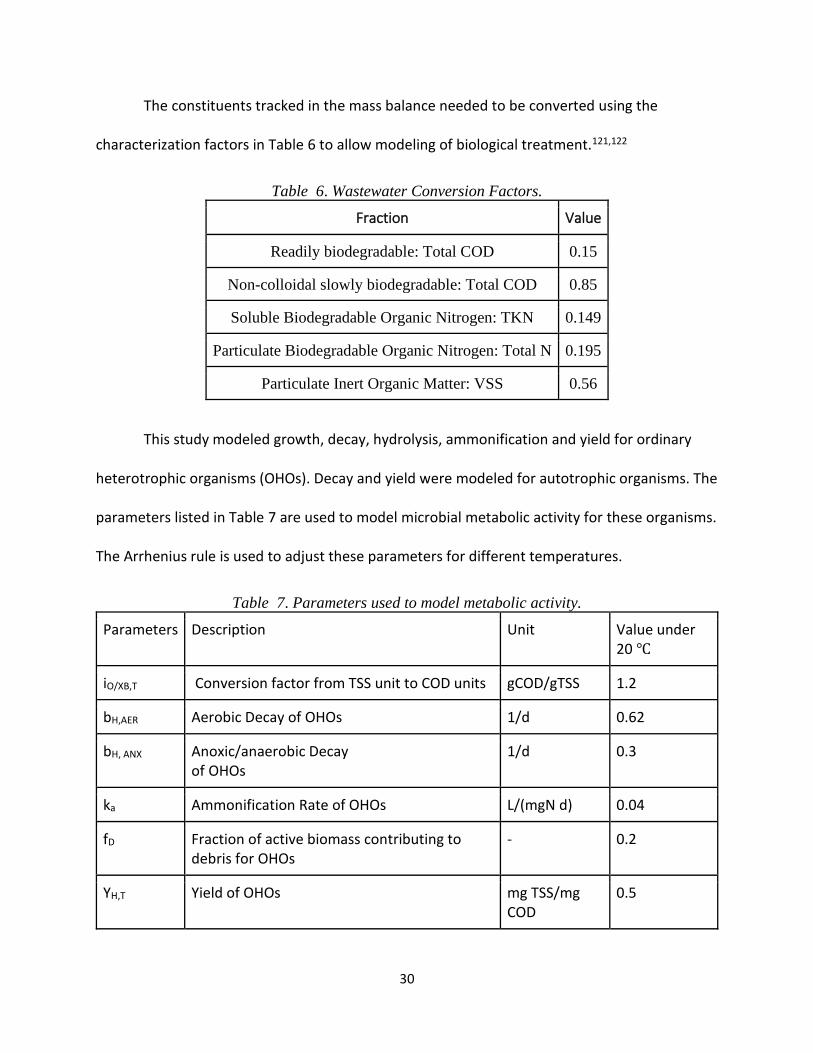
The constituents tracked in the mass balance needed to be converted using the
characterization factors in Table 6 to allow modeling of biological treatment.121,122
Table 6. Wastewater Conversion Factors.
Fraction Value
Readily biodegradable: Total COD 0.15
Non-colloidal slowly biodegradable: Total COD 0.85
Soluble Biodegradable Organic Nitrogen: TKN 0.149
Particulate Biodegradable Organic Nitrogen: Total N 0.195
Particulate Inert Organic Matter: VSS 0.56
This study modeled growth, decay, hydrolysis, ammonification and yield for ordinary
heterotrophic organisms (OHOs). Decay and yield were modeled for autotrophic organisms. The
parameters listed in Table 7 are used to model microbial metabolic activity for these organisms.
The Arrhenius rule is used to adjust these parameters for different temperatures.
Table 7. Parameters used to model metabolic activity.
Parameters Description Unit Value under 20 ℃
iO/XB,T Conversion factor from TSS unit to COD units gCOD/gTSS 1.2
bH,AER Aerobic Decay of OHOs 1/d 0.62
bH, ANX Anoxic/anaerobic Decay of OHOs
1/d 0.3
ka Ammonification Rate of OHOs L/(mgN d) 0.04
fD Fraction of active biomass contributing to debris for OHOs
- 0.2
YH,T Yield of OHOs mg TSS/mg COD
0.5

31
bA Autotrophic decay 1/d 0.17
YA,T Yield of autotrophic organisms mg TSS/mg COD
0.15
This study modeled growth, decay, hydrolysis, ammonification and yield for ordinary
heterotrophic organisms (OHOs). Decay and yield were modeled for autotrophic organisms. The
parameters listed in Table 8 are used to model microbial metabolic activity for these organisms.
The Arrhenius rule is used to adjust these parameters for different temperatures.
Table 8. Parameters used to model metabolic activity.
Parameters Description Unit Value under
20 ℃
iO/XB,T Conversion factor from TSS unit to COD
units
gCOD/gTSS 1.2
bH,AER Aerobic Decay of OHOs 1/d 0.62
bH, ANX Anoxic/anaerobic Decay
of OHOs
1/d 0.3
ka Ammonification Rate of OHOs L/(mgN d) 0.04
fD Fraction of active biomass contributing to
debris for OHOs
- 0.2
YH,T Yield of OHOs mg TSS/mg
COD
0.5
bA Autotrophic decay 1/d 0.17
YA,T Yield of autotrophic organisms mg TSS/mg
COD
0.15
B2.2 Effluent Quality
B2.2.1 COD, Total Phosphorus, Ammonia-Nitrogen
32
The rule-based model used for this study continued treatment until the concentration of
all regulated contaminants were at or below regulatory levels. This determined important
operating characteristics such as the solids retention time or the treatment plant configuration.
The effluent COD concentration is assumed to be equal to the effluent standard.
In cases where the influent concentration of phosphorus is less than the effluent standard,
the effluent concentration is determined by the phosphorus in the influent and the phosphorus
removed by biomass production. When the secondary influent is in excess of the effluent
standard, the effluent concentration is assumed to be equal to the effluent standard. Phosphorus is
removed by either biological methods, chemical methods, or both.
Systems with anaerobic zones (e.g. the Five-Stage Bardenpho treatment plant in the
Virginia scenario) use Phosphorus-Accumulating Organisms (PAOs) to remove phosphorus. It is
assumed that 10.7 grams of Volatile Fatty Acids as COD are required to remove one gram of
phosphorus.122 If there is not enough volatile fatty acids to remove the required phosphorus
biologically or if the treatment plant does not use biological phosphorus removal, the remaining
phosphorus requiring removal is precipitated with ferric chloride.
When the concentration of ammonia-nitrogen in the influent is lower than the effluent
standard, the effluent concentration is assumed to be equal to the influent concentration. When
the concentration of ammonia-nitrogen is higher than the effluent standard, nitrification is
induced and the concentration is assumed to be equal to the effluent standard.
B2.2.2 Nitrate and Total Nitrogen
Nitrate formed during nitrification
33
The treatment plant modeled for the Virginia scenario and some of the treatment plants
modeled for the Michigan scenario use nitrification and denitrification to reduce the
concentration of total nitrogen in the effluent. First, the concentration of nitrate formed during
nitrification is calculated using equation 1.122
𝑆𝑁𝑂 = 0.98(𝑆𝑁,𝑎 − 𝑆𝑁𝐻 − 𝑆𝑁𝑆) (equation 1)
Where: 𝑆𝑁𝑂=Nitrate Formed by nitrification
𝑆𝑁,𝑎=Nitrogen available to nitrifiers
𝑆𝑁𝐻=Effluent Ammonia Nitrogen concentration, set as the effluent standard
𝑆𝑁𝑆=Effluent soluble organic N concentration
The concentration of nitrogen available to nitrifiers is calculated using equation 2.122
𝑆𝑁,𝑎 = 𝑆𝑁𝐻0 + 𝑆𝑁𝑆0 + 𝑋𝑁𝑆0 − 𝑁𝑅(𝑆𝑆0 + 𝑋𝑆0 − 𝑆𝑆) (equation 2)
Where: 𝑆𝑁𝐻0= influent soluble ammonia N concentration
𝑆𝑁𝑆0= soluble biodegradable N concentration
𝑋𝑁𝑆0= particulate biodegradable organic N concentration
𝑁𝑅= Nitrogen required for heterotroph growth
𝑆𝑆0= influent readily biodegradable COD concentration
𝑋𝑆0= influent slowly biodegradable COD concentration
𝑆𝑆= effluent COD concentration, which is determined by standard
Equation 3 is used to determine the nitrogen required for heterotroph growth.122
𝑁𝑅 = 0.087(1+𝑓𝐷𝑏𝐻𝑆𝑅𝑇𝐼𝐴𝑍+𝑃𝐴𝑍)𝑌𝐻,𝑇𝑖𝑂/𝑋𝐵,𝑇
(1+𝑏𝐻𝑆𝑅𝑇𝐼𝐴𝑍+𝑃𝐴𝑍) (equation 3)
Where: 𝑆𝑅𝑇𝐼𝐴𝑍+𝑃𝐴𝑍=Solids Retention time of the initial anoxic zone and the primary aerobic
zone, days

34
Denitrification
The Modified Ludzack-Ettinger (MLE) treatment plants that were a part of the Michigan
scenario had denitrification in one zone. The Five-Stage Bardenpho plant modeled for the
Virginia scenario had denitrification in two zones. Some of the processes to model the initial
anoxic zone for the Five-Stage Bardenpho plant and the only anoxic zone for the MLE are
described below. Then, the processes to model the second denitrification zone for the Five-Stage
Bardenpho plant will be described.
Denitrification in the Initial Anoxic Zone
Both readily and slowly biodegradable substrate are assumed to be available for
denitrification due to a long enough Solids Retention Time (>3 days). External carbon sources
such as methanol are added when there is not enough biodegradable substrate for nitrate
removal.
Denitrification associated with both slowly biodegradable substrate and denitrification
associated with readily biodegradable substrate are included. Equation 4 is used to estimate the
mass rate of denitrification associated with utilization of slowly biodegradable substrate. The
concentration of the Mixed Liquor Suspended Solids (MLSS) is assumed to be 3,500 grams of
TSS per cubic meter.
∆𝑁𝑋𝑆 = 𝑞𝑁𝑂/𝑋𝑆𝑀𝐿𝑆𝑆𝐼𝐴𝑍 (equation 4)
Where: 𝑁𝑋𝑆= mass rate of denitrification, grams nitrate-N per day
𝑞𝑁𝑂/𝑋𝑆=Specific Nitrate-N Utilization Rate, grams nitrate-N per gram MLSS per day
𝑀𝐿𝑆𝑆𝐼𝐴𝑍=Concentration of MLSS in the Initial Anoxic Zone

35
The specific nitrate-N utilization rate associated with slowly biodegradable COD is
calculated using equation 5.
𝑞𝑁𝑂/𝑋𝑆 = 0.018𝑈𝐴𝑁𝑋 + 0.029
(equation 5)
Where: 𝑈𝐴𝑁𝑋= the loading factor for slowly biodegradable substrate to the anoxic zone
The loading factor for slowly biodegradable substrate to the anoxic zone (UANX) is
calculated using Equation 6.
𝑈𝐴𝑁𝑋 = 𝐹 ∙ 𝑆𝑆0 ∙ 𝑀𝐿𝑆𝑆𝐼𝐴𝑍 (equation 6)
Where: 𝑀𝐿𝑆𝑆𝐼𝐴𝑍=Mixed Liquor Suspended Solids in the initial anoxic zone
The denitrification rate associated with readily biodegradable substrate is calculated using
equation 7. Then, the effluent nitrate concentration from the primary aerobic zone (CN1) is
calculated using equation 8.
∆𝑁𝑆𝑆 = 𝐹 ∙ 𝑆𝑆01−𝑌𝐻,𝑇𝑖𝑂𝑖𝑂/𝑋𝐵,𝑇
2.86 (equation 7)
𝐶𝑁1 = 𝑆𝑁0 − ∆𝑁𝑋𝑆 − ∆𝑁𝑆𝑆 (equation 8)
Denitrification in the Secondary Anoxic Zone
For the secondary anoxic zone, the Burdick empirical relationship (eq. 9) is used to
estimate the specific denitrification rate.
𝑞𝑁𝑂/𝑋𝐵 = 0.12𝑆𝑅𝑇𝑇𝑂𝑇−0.706 (equation 9)
This is then used in equation 10 to estimate the denitrification mass rate.
36
∆𝑁𝑋𝐵 = 𝑞𝑁𝑂/𝑋𝐵𝑀𝐿𝑆𝑆𝑆𝐴𝑍 (equation 10)
Where: 𝑀𝐿𝑆𝑆𝑆𝐴𝑍= Concentration of Mixed Liquor Suspended Solids in the secondary anoxic
zone
The effluent loads of these species and TRACI impact factors are used to determine the
eutrophication potential of wastewater. 123
B2.3 Direct Greenhouse Gas Emissions
Wastewater treatment can lead to considerable emissions of carbon dioxide and nitrous
oxide. This study did not estimate direct emissions of carbon dioxide under the assumption that
they are predominately biogenic, and that urine diversion will not affect the amount of carbon
dioxide from fossil origin. In reality, this is a conservative approach because urine diversion may
decrease direct carbon dioxide emissions because it can decrease the input of fossil carbon
inputs, such as methanol.
Nitrous oxide emissions have been observed in treatment plants that utilize nitrification
and denitrification. Nitrous oxide emitted during wastewater treatment and after wastewater is
released in the environment can be found in Table 10. It is worth noting that nitrous oxide
emissions are very uncertain, and different methodologies have been used in other studes.121,124–
126
B2.4 Electricity Consumption
B2.4.1 Oxygen Demand
Aeration is one of the largest environmental impacts of wastewater treatment, and be
significantly affected by the concentration of nutrients in wastewater. As shown in equation 11,

37
the total oxygen demand depends on the oxygen demand of heterotrophic and autotrophic
organisms.
𝑅𝑂𝑡𝑜𝑡 = 𝑅𝑂𝐻 + 𝑅𝑂𝐴 (equation 11)
Equation 12 is used to calculate the oxygen demand from heterotrophic organisms. This
is determined by the amount of COD removed and metabolic characteristics of these organisms.
𝑅𝑂𝐻 = 𝐹(𝑆𝑆0 + 𝑋𝑆0 − 𝑆𝑆) [1 −(1+𝑓𝐷𝑏𝐻𝑆𝑅𝑇𝑇𝑂𝑇)𝑌𝐻,𝑇𝑖𝑂/𝑋𝐵,𝑇
1+𝑏𝐻𝑆𝑅𝑇𝑇𝑂𝑇] (equation 12)
Where: 𝐹=m3 wastewater treated per day
𝑆𝑆0=Influent readily biodegradable COD
𝑋𝑆0=Influent slowly biodegradable COD
𝑆𝑆= Effluent COD
Treatment plants with ammonia effluent standards also require considerable quantities of
oxygen to support autotrophic organisms. In those instances, equation 13 is used to quantify the
oxygen demand of these organisms.
𝑅𝑂𝐴 = 𝐹(𝑆𝑁,𝑎 − 𝑆𝑁𝐻) [4.57 −(1+𝑓𝐷𝑏𝐴𝑇𝑂𝑇𝑆𝑅𝑇𝑇𝑂𝑇)𝑌𝐴,𝑇𝑖𝑂/𝑋𝐵,𝑇
1+𝑏𝐴𝑆𝑅𝑇𝑇𝑂𝑇] (equation 13)
B2.4.2 Other Electricity Demand
Electricity is also consumed for mixing and pumping wastewater. For both anaerobic and
anoxic zones, it is assumed that 5 watts per cubic meter of reactor volume is needed. It is
assumed that influent wastewater, Return Activated Sludge (RAS), Mixed Liquor Recirculation
(MLR), and Waste Activated Sludge (WAS) are pumped at 70% efficiency with head losses
described in Table 9.
38
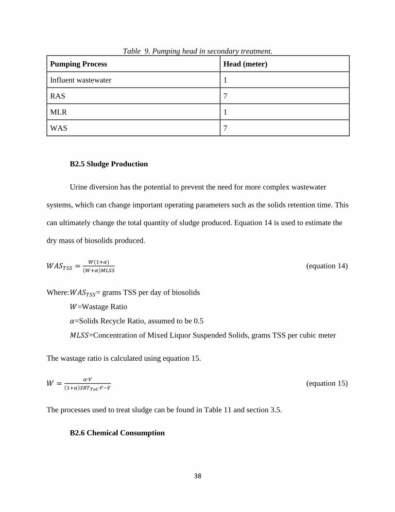
Table 9. Pumping head in secondary treatment.
Pumping Process Head (meter)
Influent wastewater 1
RAS 7
MLR 1
WAS 7
B2.5 Sludge Production
Urine diversion has the potential to prevent the need for more complex wastewater
systems, which can change important operating parameters such as the solids retention time. This
can ultimately change the total quantity of sludge produced. Equation 14 is used to estimate the
dry mass of biosolids produced.
𝑊𝐴𝑆𝑇𝑆𝑆 =𝑊(1+𝛼)
(𝑊+𝛼)𝑀𝐿𝑆𝑆 (equation 14)
Where: 𝑊𝐴𝑆𝑇𝑆𝑆= grams TSS per day of biosolids
𝑊=Wastage Ratio
𝛼=Solids Recycle Ratio, assumed to be 0.5
𝑀𝐿𝑆𝑆=Concentration of Mixed Liquor Suspended Solids, grams TSS per cubic meter
The wastage ratio is calculated using equation 15.
𝑊 =𝛼∙𝑉
(1+𝛼)𝑆𝑅𝑇𝑇𝑜𝑡∙𝐹−𝑉 (equation 15)
The processes used to treat sludge can be found in Table 11 and section 3.5.
B2.6 Chemical Consumption

39
This study included chemical consumption for phosphorus removal, disinfection,
alkalinity adjustment, and external carbon addition. Ferric chloride was used to precipitate
phosphorus. The amount of phosphorus requiring chemical precipitation is described in section
2.2.2.1. Sodium hypochlorite was assumed to be the disinfectant used in all wastewater treatment
plants. The dosage used for both can be found in Table 10. Lime was used for alkalinity
adjustment, and methanol was used as the external source of carbon. The dosage for each
chemical depends on the biological processes occurring during treatment and are described
below.
B2.6.1 Alkalinity Adjustment with Lime
The assumed initial alkalinity in all systems was 200 milligrams as calcium carbonate per
liter. If enough alkalinity is consumed by biological processes such as nitrification that the
alkalinity would drop below 50 milligrams as calcium carbonate per liter, lime is added. Each
gram of lime provides 1.35 grams of alkalinity as Calcium Carbonate.127
Nitrification of ammonia to nitrate consumes alkalinity.122 Equation 16 is used to
calculated alkalinity destroyed in treatment plants with nitrification but no denitrification.
𝐴𝑙𝑘𝑑𝑒𝑠 = 7.23 ∙ 𝑆𝑁0 (equation 16)
Where: 𝐴𝑙𝑘𝑑𝑒𝑠= Alkalinity destroyed, in grams per cubic meter
𝑆𝑁0=Concentration of Nitrate-N formed, in grams per cubic meter
Converting nitrate to nitrogen gas through denitrification produces alkalinity. Equation
17 is used for treatment plants with nitrification and denitrification.
𝐴𝑙𝑘𝑑𝑒𝑠 = 7.23 ∙ 𝑆𝑁0 − 3.5 ∙ (𝑆𝑁0 − 𝑆𝑁) (equation 17)

40
Where: 𝑆𝑁=Concentration of effluent Nitrate-N in grams per cubic meter, set by effluent standard
B2.6.2 External Carbon Provided from Methanol
Many treatment plants add an external carbon source to ensure a high enough carbon to
nitrogen ratio during denitrification. As shown in equation 18, this is done by finding the
difference between the ideal readily biodegradable substrate and the actual readily biodegradable
substrate. Additional substrate is provided in the form of methanol. The assumed COD of
methanol is assumed to be 1.2 kg/L.
𝑅𝑒𝑞𝑢𝑖𝑟𝑒𝑑 𝐴𝑑𝑑𝑖𝑡𝑖𝑜𝑛𝑎𝑙 𝑆𝑢𝑏𝑠𝑡𝑟𝑎𝑡𝑒 (𝑚𝑔/𝐿) = ∆𝑆𝑇𝑖 − 𝐹 ∙ 𝑆𝑆0 (equation 18)
Where: ∆𝑆𝑇𝑖=Ideal mass rate of readily biodegradable substrate for denitrification, grams per day
The ideal concentration of readily biodegradable substrate is found using the required
denitrification mass rate and yield, as shown in equation 19.
∆𝑆𝑇𝑖 =(∆𝑁𝑆𝑇+∆𝑁𝑋𝐵)
(1−𝑌𝐻,𝑇𝑖𝑂/𝑋𝐵,𝑇)/2.86 (equation 19)
Where: ∆𝑁𝑆𝑇=Required Mass Denitrification Rate from readily biodegradable COD in initial
anoxic zone
∆𝑁𝑋𝐵=Denitrification mass rate in the secondary anoxic zone
The required mass rate of denitrification associated with utilization of readily
biodegradable COD in the initial anoxic zone is determined using equation 20.
∆𝑁𝑆𝑇 = 𝐹 ∙ 𝑆𝑁𝑂 − ∆𝑁𝑋𝑆 − ∆𝑁𝑋𝐵 − 𝑊𝐴𝑆𝑇𝑁 − (𝐹 − 𝐹𝑊)𝑆𝑇𝑁,𝑒𝑓𝑓 (equation 20)

41
Where: 𝑁𝑋𝑆=Denitrification mass rate from slowly biodegradable substrate in the initial anoxic
zone
𝑊𝐴𝑆𝑇𝑁=Wastage nitrogen mass rate, grams of nitrogen per day
𝐹𝑊=Flow rate of waste sludge, cubic meters per day
𝑆𝑇𝑁,𝑒𝑓𝑓=Concentration of nitrogen in effluent, grams of nitrogen per day
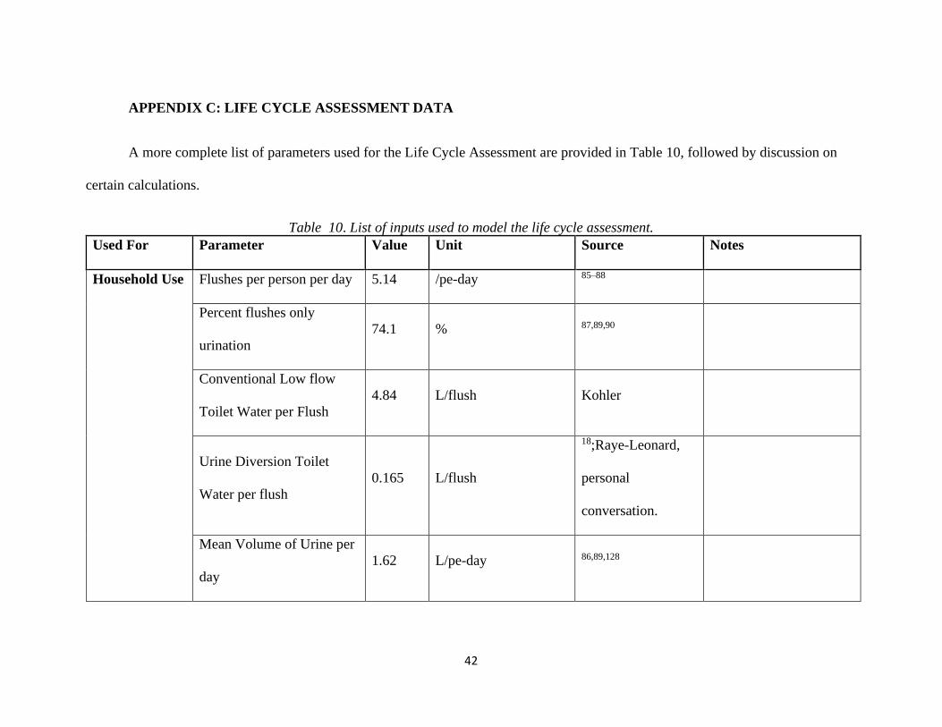
42
APPENDIX C: LIFE CYCLE ASSESSMENT DATA
A more complete list of parameters used for the Life Cycle Assessment are provided in Table 10, followed by discussion on
certain calculations.
Table 10. List of inputs used to model the life cycle assessment.
Used For Parameter Value Unit Source Notes
Household Use Flushes per person per day 5.14 /pe-day 85–88
Percent flushes only
urination
74.1 % 87,89,90
Conventional Low flow
Toilet Water per Flush
4.84 L/flush Kohler
Urine Diversion Toilet
Water per flush
0.165 L/flush
18;Raye-Leonard,
personal
conversation.
Mean Volume of Urine per
day
1.62 L/pe-day 86,89,128

43
Mean defecation volume
per day
0.233 L/pe-day 13,129
5% Acetic Acid added
(Urine Concentration)
0.0417
L/L urine and
flushwater
25
Likely more than
needed, from water with
a high pH.130
5% acetic acid added
(Struvite and Ammonium
Sulfate)
0.0330
L/L urine and
flushwater
Calculated
Water conveyance losses 13 % 9,66,131
Electricity to convey water 0.202 kWh/m3 16,44,137,64,66,80,132–136
Surface Water
Treatment
Electricity 0.443 kWh/m3 9,57,59–62,65,66,132,138
Alum 0.0491 kg/m3
Ferric Chloride 0.00425 kg/m3
Polymer
1.19۰10-
4
kg/m3
Lime 0.00493 kg/m3

44
Limestone 0.0203 kg/m3
NaOH 0.0166 kg/m3
HSF 0.0011 kg/m3
Ammonia
2.10۰10-
4
kg/m3
Phosphoric acid 0.028 kg/m3
CO2 0.0182 kg/m3
Chlorine gas 0.00148 kg/m3
Sodium hypochlorite 0.0129 kg/m3
Calcium hydroxide 0.0138 kg/m3
KMnO4
1.96۰10-
4
kg/m3
Groundwater
Treatment
Electricity 0.786 kWh/m3 48,58–60,63–65
Alum
1.15۰10-
5
kg/m3
Lime 0.0484 kg/m3
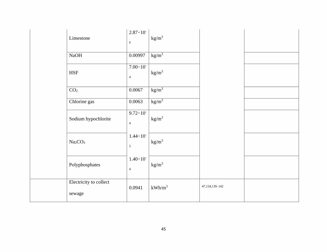
45
Limestone
2.87۰10-
6
kg/m3
NaOH 0.00997 kg/m3
HSF
7.00۰10-
4
kg/m3
CO2 0.0067 kg/m3
Chlorine gas 0.0063 kg/m3
Sodium hypochlorite
9.72۰10-
4
kg/m3
Na2CO3
1.44۰10-
5
kg/m3
Polyphosphates
1.40۰10-
4
kg/m3
Electricity to collect
sewage
0.0941 kWh/m3 47,134,139–142

46
Wastewater
Collection
energy
Urine Collection Electricity
0.202
kWh/m3
Assumed to be same as
pressurized water system
Struvite and
Ammonium
Sulfate
Production
Mg:P ratio 1.5:1 48,54,91,92
Head loss 4.6 meters Assumed
Electricity, Struvite
dewatering
0.783 kWh/kg struvite
Bott, personal
conversation
Dowex Mac adsorption
density
4.9 mole/kg resin 39,49
Sulfuric Acid (18%) per kg
N
16.7 L/kg N
Tarpeh, personal
conversation
Nitrogen concentration in
liquid Ammonium Sulfate
59 g/L 49
Resin replacement
frequency
5 years 49
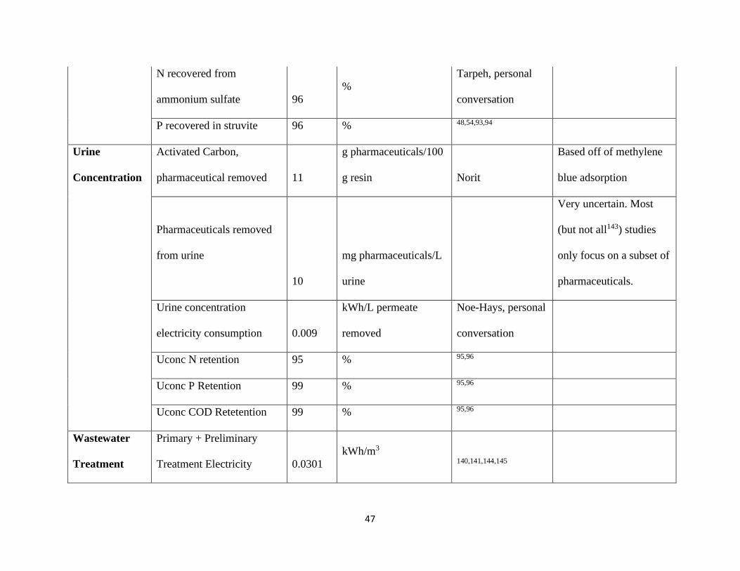
47
N recovered from
ammonium sulfate 96
%
Tarpeh, personal
conversation
P recovered in struvite 96 % 48,54,93,94
Urine
Concentration
Activated Carbon,
pharmaceutical removed 11
g pharmaceuticals/100
g resin Norit
Based off of methylene
blue adsorption
Pharmaceuticals removed
from urine
10
mg pharmaceuticals/L
urine
Very uncertain. Most
(but not all143) studies
only focus on a subset of
pharmaceuticals.
Urine concentration
electricity consumption 0.009
kWh/L permeate
removed
Noe-Hays, personal
conversation
Uconc N retention 95 % 95,96
Uconc P Retention 99 % 95,96
Uconc COD Retetention 99 % 95,96
Wastewater
Treatment
Primary + Preliminary
Treatment Electricity 0.0301
kWh/m3 140,141,144,145
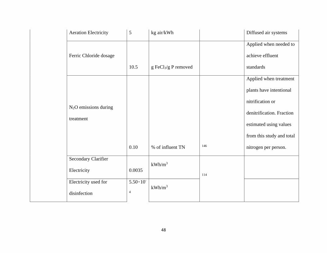
48
Aeration Electricity 5 kg air/kWh
Diffused air systems
Ferric Chloride dosage
10.5 g FeCl3/g P removed
Applied when needed to
achieve effluent
standards
N2O emissions during
treatment
0.10 % of influent TN 146
Applied when treatment
plants have intentional
nitrification or
denitrification. Fraction
estimated using values
from this study and total
nitrogen per person.
Secondary Clarifier
Electricity 0.0035
kWh/m3
114
Electricity used for
disinfection
5.50۰10-
4
kWh/m3
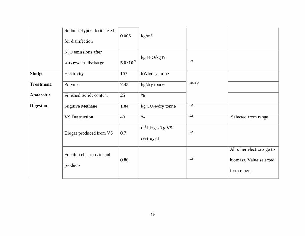
49
Sodium Hypochlorite used
for disinfection
0.006 kg/m3
N2O emissions after
wastewater discharge 5.0۰10-3
kg N2O/kg N 147
Sludge
Treatment:
Anaerobic
Digestion
Electricity 163 kWh/dry tonne
148–152
Polymer 7.43 kg/dry tonne
Finished Solids content 25 %
Fugitive Methane 1.84 kg CO2e/dry tonne 152
VS Destruction 40 % 122 Selected from range
Biogas produced from VS 0.7
m3 biogas/kg VS
destroyed
122
Fraction electrons to end
products
0.86 122
All other electrons go to
biomass. Value selected
from range.
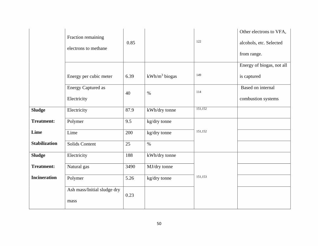
50
Fraction remaining
electrons to methane
0.85 122
Other electrons to VFA,
alcohols, etc. Selected
from range.
Energy per cubic meter 6.39 kWh/m3 biogas 149
Energy of biogas, not all
is captured
Energy Captured as
Electricity
40 % 114
Based on internal
combustion systems
Sludge
Treatment:
Lime
Stabilization
Electricity 87.9 kWh/dry tonne 151,152
Polymer 9.5 kg/dry tonne
151,152
Lime 200 kg/dry tonne
Solids Content 25 %
Sludge
Treatment:
Incineration
Electricity 188 kWh/dry tonne
151,153
Natural gas 3490 MJ/dry tonne
Polymer 5.26 kg/dry tonne
Ash mass/Initial sludge dry
mass
0.23

51
Sludge
Treatment:
Thermal
Drying
Electricity 242 kWh/dry tonne
150,152
Natural Gas 11400 MJ/dry tonne
Polymer 7.83 kg/dry tonne
Solids content 90 %
Sludge
Treatment:
Composting
Electricity 97.8 kWh/dry tonne
150–152
Diesel Consumption in
facility
2.83 L/dry tonne
Polymer 7.33 kg/dry tonne
Sludge End of
Life:
Transportation
Distance sludge shipped to
land application
20 km
Class 8 truck, empty
backhaul
Distance sludge shipped to
landfill
52 km
Class 8 truck, empty
backhaul
Sludge End of
Life: Applying
Compost
Diesel Consumption 2.68 L/dry tonne 152
N2O emissions from
application
0.316 kg N2O/dry tonne 152
Carbon Sequestered 250 kg CO2e/dry tonne 152

52
N Fertilizer Offset 160 kg CO2e/dry tonne 152
P Fertilizer Offset 30 kg CO2e/dry tonne 152
Diesel Consumption 2.68 L/dry tonne 152
P emitted to water
0.2
kg/tDM 154
Methane Emission
(storage)
18 kg CO2e/dry tonne 152
Sludge End of
Life: Land
Application
N2O emissions from
application 12.8
kg CO2e/dry tonne 152
Ammonia emitted to air 1.14 kg/tDM 154
P emitted to water 0.2 kg/tDM 154
Carbon Sequestered 250 kg CO2e/dry tonne 152
N Fertilizer Offset 200 kg CO2e/dry tonne 152
P Fertilizer Offset 38 kg CO2e/dry tonne 152
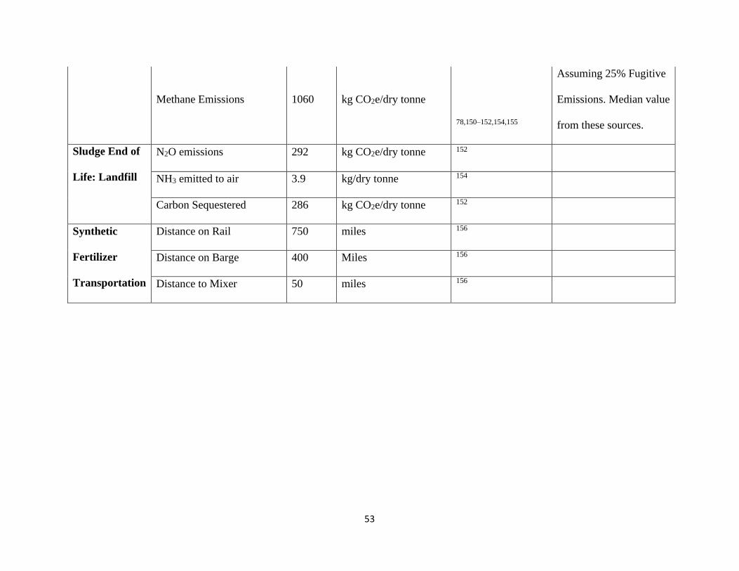
53
Methane Emissions 1060 kg CO2e/dry tonne
78,150–152,154,155
Assuming 25% Fugitive
Emissions. Median value
from these sources.
Sludge End of
Life: Landfill
N2O emissions 292 kg CO2e/dry tonne 152
NH3 emitted to air 3.9 kg/dry tonne 154
Carbon Sequestered 286 kg CO2e/dry tonne 152
Synthetic
Fertilizer
Transportation
Distance on Rail 750 miles 156
Distance on Barge 400 Miles 156
Distance to Mixer 50 miles 156
54
C1 Transporting Materials
Environmental burdens of hauling materials from the location of production to the
municipality were included. Fuel consumption for transportation of all chemicals, activated
carbon, biosolids, and urine-derived fertilizer was estimated using equation 21. All were
assumed to be transported with an empty backhaul. This equation was used to account for the
distance that synthetic fertilizers were transported via truck, while USLCI data were used for rail
and barge transportation.82
𝐹𝐶 = (𝐹𝑅𝑉 ∙ 𝑀𝑔𝑣 + 𝐾) ∙ 𝐷 + (𝐹𝑅𝑉 ∙ 𝑀𝑣ℎ + 𝐾) ∙ 𝐷 (equation 21)
Where: FC = Fuel Consumption, gallons
FRV = Fuel Reduction Value, 0.238 gallons diesel/100 t-mi
Mgv = Gross Vehicle Mass, 40 short tons
Mvh = Mass of vehicle and trailer, 17.5 short tons
K = 9.7 gallons/100 mi
D = Distance (in 100 mi)
The distance that urine-derived fertilizers and activated carbon were shipped varied
between scenarios, while the distance that chemicals were shipped did not. For each scenario,
distances urine-derived fertilizers were shipped were estimated by mapping distances from some
wastewater treatment plants in the state to large fertilizer suppliers. Assumed distances that
chemicals were shipped were informed by the locations of wastewater treatment plants and
locations of chemical production plants. These locations were often found using sources such as
the NSF Certified Drinking Water Treatment Chemicals database.157

55
C2 Household Activities
C2.1 Environmental Burdens of Potable Water
This study differentiated water production in each scenario by considering the ratio of
groundwater and surface water. While this is just one of many factors that may affect the
environmental impacts of treating potable water, it is useful as a high-level analysis between
states.59,158 Different LCAs were used to determine the inputs per cubic meter of groundwater
and surface water found in Table 10.48,56,65–67,138,57–64 This required weighting inputs found in
different studies, which will be described below. Then, the inputs of surface and groundwater
were applied in the relevant ratios to characterize a composite cubic meter of water.55
Some studies on potable water treatment only quantified energy, while others quantified
energy and chemicals consumed. Because of this, different weightings were needed for energy
and chemical consumption.
For the electricity consumption of surface water, half of the weight was assigned to
values reported in the EPRI report because it was a broad survey focused on the U.S., as opposed
to focusing on individual water treatment plants.59 The electricity consumption in each of the
other surface water treatment LCAs was given a weight of 6.25%.57,61,62,67,138 Chemical
consumption was based off of the four studies that quantified chemical use.58,60,61,65 Each were
evenly weighted.
Fewer LCAs on groundwater treatment were found. For electricity consumption, the
EPRI report was once again given half of the total weight,59 while the remaining sources were
each given a weight of 12.5%.48,58,60,63,64 Only three sources contained usable data on chemical
consumption. The moderate softening scenario in Godskesen et al. was given a weighting of
20%, the Ishii & Boyer inventory was given a weighting of 35% because it assesses water

56
treatment in the US, and the inventory in the Renzoni & Germain study was given a weighting of
45% because this contained an average value.
C2.2 Water and Acetic Acid for Flushing
The quantities of water and acetic acid used for flushing are listed in Table 10. Table 11
provides further description of when each type of flush is used. Feces only flushes are estimated
to only comprise 2% of total flushes and are lumped together with urine and feces flushes.87
When a user both urinated and defecated, it was assumed that the urine was separated from the
feces using a toilet similar to a NoMix toilet.159 Because this study assumed urine-diversion is
very common, it was assumed that users were used to the concept and used the toilets properly
without issues found in early studies on urine diversion.109,160 The nutrient composition of urine
and feces were obtained from the literature.114,115,117,118
Table 11. Description of flush volumes.
Urine Diversion Alternatives Conventional
Alternative
70% of population diverting
urine
30% of
population not
diverting urine
Entire Population
Urine only Urine and
Feces
All Flushes All Flushes
UD Flush Low-flow flush
+ UD Flush
Low-flow
flush
Low-flow flush
Acetic acid is needed in both urine diversion alternatives to delay the process of
hydrolysis, which can cause precipitation from urine and can clog pipes.15,28 The struvite and
ammonium sulfate scenario uses less acetic acid because a higher pH is needed to precipitate
struvite. It was assumed each flush would provide enough acetic acid to neutralize the alkalinity
of urine, which is described in equation 22. The pH of fresh urine is assumed to be 6.2,27–29 and
57
the concentration of ammonia and phosphate were determined from the nutrient composition of
urine. It is assumed that nutrients in potable water were negligible compared to urine.
Alkalinity of urine stream=-[H+]+[OH-]+[NH3]+2[PO43-] (Equation 22)
The amount of acetic acid needed for the urine concentration was determined through a
pilot scale system at the University of Michigan. It should be noted that this location’s potable
water has a high pH of 9.3130, which may result in an overestimation of how much acetic acid is
required.
C3 Conveyance of Urine
Urine collections is modeled as if it were collected in a pressurized pipe system. The
electricity consumption for potable water was deemed as a reasonable estimate. The pipes would
be smaller, which would increase head loss. Unlike water, urine collection pipes will not need to
be designed to fight fires, reducing required pressure. In addition, they might follow the pathway
of sewage collection systems, which already take advantage of gravity.
C4 Urine Derived Fertilizer Production
C4.1 Struvite and Ammonium Sulfate
Struvite is the first fertilizer produced. After the diverted urine arrives at the production
center, magnesium oxide is mixed in to provide magnesium and to raise the pH, which causes
most of the phosphorus to precipitate as struvite. The precipitated struvite is then dried through
draining, an electric dryer, a bucket elevator, and then a vibratory screen (Bott, personal
conversation). The effluent from this process continues to ion exchange.
After struvite is precipitated, ion exchange is used to remove the nitrogen and produce a
fertilizer. The effluent urine from struvite production is pumped through vessels containing an

58
ion exchange resin such as Dowex Mac 3 resin.39,49 The ion exchange cartridge collects the
ammonia from the urine.39 To regenerate a cartridge, 18% sulfuric acid is pumped through the
filter, which extracts the ammonia and produces a liquid ammonium sulfate fertilizer.49 Head
loss in the cartridge was estimated using the hydraulic conductivity and common column heights.
It was assumed that each urine-derived fertilizer production facility always had enough
ion exchange resin to where nitrogen could be removed for 7 days without exceeding the
adsorption capacity. The lifetime of the resin is assumed to be 5 years.49 The environmental
burdens of ion exchange resin were not available, so polystyrene was used because it the
backbone of the resin.161
C4.2 Urine Concentration
The urine concentration scenario removes pharmaceuticals, concentrates urine and
deactivates pathogens. While the impacts of pharmaceuticals are not assessed in this study, the
inputs for removing them using activated carbon are. The activated carbon is assumed to be
shipped back to a regeneration center as a slurry with a 30% solids concentration. A weighted
average for the inputs needed to thermally regenerate activated carbon was determined through
the literature, and it was assumed that 10% of activated carbon was lost per regeneration.69–72 It
was assumed that each urine-derived fertilizer plant had enough activated carbon to allow
continuous removal of pharmaceuticals for 1.1 years.
Urine is concentrated five times its original concentration using reverse osmosis. It was
assumed that the membrane received an acid and alkaline wash every six months. The inputs
were obtained from a Hydranautics technical report73. The only equipment and maintenance
considered were the production of and cleaning of the membrane. The necessary area of
59
membrane was based off of the flow rate and the area per influent volume found in other
studies.162–164 A three year membrane lifetime was assumed.
All urine derived fertilizers were assumed to be transported from the fertilizer production
facility to regional fertilizer distributers using class 8 trucks with an empty backhaul. Each trip
was assumed to haul 22.5 short tons of fertilizer.
C4.3 Synthetic Fertilizer
Synthetic fertilizers were used for the conventional alternatives and to ensure all
alternatives (including urine diversion) provided the same mass of nitrogen and phosphorus as
fertilizer. Equal mass of nutrients was deemed functionally equivalent because previous research
did not find a significant difference in nutrient uptake between these fertilizer alternatives.25,75–77
The synthetic fertilizers produced were mono-ammonium phosphate (phosphorous and some
nitrogen) and urea (nitrogen). Both are commonly used in the U.S.99
The urine concentration alternative retains the most phosphorus, and was used to
determine how much phosphorus is needed in each alternative. The struvite and ammonium
sulfate alternative retained the most nitrogen, and was used to determine how much urea was
needed in the other alternatives.
C5 Sludge Treatment
Primary sludge is excluded from the scope of this study because it is assumed that urine
diversion will not affect the amount produced or how it is treated. This study does model
treatment of the sludge produced from biological wastewater treatment and its disposal.

60
All secondary sludge is assumed to be thickened, dewatered, and stabilized. In all
scenarios, sludge was treated in a combination of anaerobic digestion, composting, lime
stabilization, incineration, and thermal drying representative of the state. It is assumed that
anaerobic digestion, composting, and lime stabilization produce sludge with 25% solids. It is
assumed that thermally drying results in sludge with 90% solids. All sources described treating
mixed sludge from primary and secondary treatment. Electricity from biogas production in
anaerobic digestion is estimated using equation 23.
𝐸𝐸𝑙𝑒𝑐𝑡𝑟𝑖𝑐𝑖𝑡𝑦 = 𝑉𝑆 ∙ 𝑅𝐷,𝑉𝑆 ∙ (1 − 𝑌𝑒,𝑏) ∙ (1 − 𝑌𝑒,𝑣) ∙ 𝑃𝑏 ∙ 𝐸𝑏𝑖𝑜𝑔𝑎𝑠 ∙ 𝑒𝑒𝑙𝑒𝑐𝑡𝑟𝑖𝑐𝑖𝑡𝑦 (equation 23)
Where: EElectricity = Electricity created from biogas, kWh
VS = kg Volatile Solid produced from wastewater treatment and sent to anaerobic
digestion
RD,VS = Ratio of Volatile Solids destroyed
Ye,b = Ratio of elections used for biomass production
Ye,v = Ratio of remaining elections used to produce VFAs and other alcohols
Pb = Production of biogas per kg VS destroyed
Eb = Energy per m3 of biogas
eelectricity = Efficiency of converting biogas to electricity
The treated sludge or ash is then shipped to the end of life. The energy use, credits such
as fertilizer displacement and carbon sequestration, and emissions to air and water are listed in
Table 10. It should be noted that estimates for fugitive methane emissions from landfills varied
multiple orders of magnitude.150–152,154,155

61
C6 Data Sources for Unit Processes
Table 12 lists which Life Cycle Databases were used for specific unit processes. GREET
was preferably used for electricity and transportation, USLCI was preferably used for other unit
processes, and ecoinvent was used in most other cases. Data were not found for some chemicals
such as citric acid, so an input-output approach was used in those cases. Data on freshwater use
was obtained from Ecoinvent.
Table 12. List of data sources used to quantify environmental impacts.
Input Source Item Name Unit Notes
Electricity EPA eGRID
and GREET
kWh Grid from
eGRID, impact
factors from
GREET
Natural Gas USLCI Natural gas, combusted in industrial
boiler/US
m3
Urea ecoinvent Urea, as N, at Regional Storehouse kg N
Monoammonium
Phosphate
ecoinvent Monoammonium phosphate, as
P2O5, at regional storehouse, RER S
kg
P2O5
Acetic acid (98%) USLCI Acetic Acid, at plant/kg/RNA kg
Ferric Chloride ecoinvent Iron (III) chloride, 40% in H2O, at
plant/CH U
kg
Alum ecoinvent Aluminum sulphate, powder, at
plant/RER U
kg
Methanol USLCI Methanol, at plant/RNA kg
Lime ecoinvent Lime, hydraulic, at plant/CH U kg
Sodium
Hypochlorite
ecoinvent Sodium hypochlorite, 15% in H2O,
at plant/RER U
kg
Sodium
hexametaphosphate
ecoinvent Sodium phosphate, at plant/RER U kg
Sodium Silico
Fluoride
ecoinvent Fluosilicic acid, 22% in H2O, at
plant/US U
kg
CO2 ecoinvent Carbon dioxide liquid, at plant/RER
U
kg
Ammonia USLCI Ammonia, steam reforming, liquid,
at plant/RNA
kg
Oxygen USLCI Oxygen, liquid, at plant kg
Sodium Hydroxide USLCI Sodium hydroxide, production mix,
at plant/RNA
kg
Magnesium Oxide ecoinvent Magnesium oxide, at plant/RER U kg

62
Sulfuric Acid USLCI 1 kg Sulfuric acid, at plant/kg/RNA kg
Low-Sulfur Diesel GREET
gallon Used equation 2-
3 to calculate
diesel
consumption in a
class 8 truck.
Barge Transport USLCI Transport, barge, diesel powered/US tkm
Rail Transport USLCI Transport, train, diesel powered/US tkm
Chlorine Gas USLCI Chlorine, gaseous, prodcution mix,
at plant/RNA
kg
Phosphoric Acid ecoinvent Phosphoric acid, industrial grade,
85% in H2O, at plant
kg
Sodium Carbonate ecoinvent sodium carbonate from ammonium
chloride production, at plant/kg/GLO
kg
Potassium
Permanganate
ecoinvent Potassium permanganate, at
plant/RER U
kg
Resin ecoinvent Polystyrene, general purpose, at
pant, CTR/kg/RNA
kg
Fiberglass ecoinvent Glass fibre, at plant/RER U kg
Activated Carbon Agrifootprint 1 kg Activated carbon, at plant/RER
Economic
kg
Citric Acid USA Input
Output
Database
Other basic organic chemical
manufacturing
US $
STPP (kg) (sodium
tripolyphosphate
ecoinvent 1 kg Sodium tripolyphosphate, at
plant/RER U
kg
Na-DDBS (kg) USA Input
Output
Database
Soap and other detergents US $
Membrane ecoinvent Polyvinylidenchloride, granulate, at
plant RER U
kg PVDF not
available165
C7 Life Cycle Impact Assessment
The Life Cycle Impact Assessment was conducted using global warming potential
(GWP), cumulative energy demand (CED), freshwater use (Water), eutrophication potential
(EP), and acidification potential (AP) as indicators. Freshwater use is technically an inventory
approach that is calculated by summing the water utilization and consumption for each unit
63
process.84 Whenever possible, this was measured on Ecoinvent, even if other impacts for a unit
process were determined using another database.83 This was selected over impact assessment
methods such as water deprivation for two main reasons. The first reason is that it would be
difficult to determine the origin of all supplies when evaluating multiple states. This would make
selection of a water stress index value highly uncertain. The second reason is to allow this
framework to be easily applied in other locations. Including an impact method that requires
geographic specificity inhibits this research goal.

64
APPENDIX D: SCENARIOS MODELED
D1 Scenario Description
The environmental merits and drawbacks of urine diversion will heavily depend on many
location specific factors. To evaluate the environmental performance of urine diversion, three
diverse locations were modeled as distinct scenarios. In each of these scenarios, all three
alternatives were evaluated.
The Vermont scenario highlights the performance of urine diversion in a region with
electricity produced from predominately renewable sources, and wastewater treatment plants that
remove phosphorus but do not remove nitrogen. This scenario based its wastewater treatment off
of a community serving approximately 25,000 residents.
The Michigan scenario considers urine diversion through a broader range of
municipalities and has an electricity grid comprised predominately of fossil fuels. This scenario
produces an “average” treatment plant by placing the state’s treatment plants into four categories
and considering the volume of wastewater treated in each. All have strict phosphorus removal
standards, while the level of ammonia and nitrogen removal varies between categories.
The Virginia scenario was selected to consider urine diversion in a location with strict
nitrogen and phosphorus limits. As many regions look to enact more stringent effluent limits,
these plants could benefit the most operationally. This scenario was based off of a treatment
plant in the Chesapeake Bay region treating wastewater for 350,000 people.
The scenarios vary factors such as the electricity grid, how water is produced, wastewater
effluent limits, sludge treatment and disposal methods, transportation distances, and temperature.

65
D2 Electricity Production
Data on the ratio of fuels used in the electricity grid and the electricity lost in
transmission were obtained from EPA eGRID.166 The Greenhouse Gases, Regulated Emissions,
and Energy Use in Transportation (GREET) Model was then used to determine the net impact of
obtaining these fuels, processing these fuels, and combusting them.167 The impact per kWh
generated is listed in Table 13.
Table 13. Environmental impacts of electricity production.
Global
Warming
Potential
Cumulative
Energy
Demand
Water
Consumption
Eutrophication
Potential
Acidification
Potential
Scenario
kg CO2-
eq/kWh MJ/kWh m3/kWh kg N-eq/kWh
kg SO2-
eq/kWh
Vermont 0.107 6.45 7.68۰10-5 1.04۰10-5 2.96۰10-4
Michigan 0.544 8.08 1.54۰10-4 1.70۰10-5 1.26۰10-3
Virginia 0.450 8.14 1.42۰10-3 1.74۰10-5 8.02۰10-4
D3 Water Sources
Table 14 shows the ratio of surface and groundwater used in the public supply for each
state.55 This ratio was multiplied by the inputs for each type of water source for a composite
cubic meter of water.
Table 14. Sources of Potable Water by Location.
Percentages used with the potable water inventories to create water inventories in each
scenario.
Water Source Michigan Vermont Virginia
Surface Water 81% 63% 88%
Groundwater 19% 37% 12%
D4 Wastewater Treatment

66
Effluent standards for each scenario were determined through assessing technical reports
from each state considered.168 These effluent standards are shown in Table 15. The Virginia and
Vermont scenarios focused on one type of treatment plant, while the Michigan scenario
evaluated the treatment plants in the state to make an “average” treatment plant. Relevant real
wastewater treatment plants were used to select the numbers of basins, solid retention time,
MLSS concentration, and secondary clarifier area.
Table 15. Effluent Wastewater Standard for input in Each Location.
All constituents are listed in milligrams per liter.
* Treatment plants with denitrification had a nitrate limit of 3 milligrams of nitrate-N per liter.
** Treatment plants with nitrification had an ammonia limit 8 milligrams of ammonia-N per
liter.
Components Michigan Vermont Virginia
BOD5 25 25 5
TSS 30 20 6
Nitrate-N -* - 3
Ammonia-N -** - 1
TP 0.7 0.2 0.18
In the Vermont scenario, the Rutland wastewater treatment plant was modeled, which has
an aerobic zone for COD removal and adds ferric chloride to remove phosphorus.
The Michigan scenario produced an “average” treatment plant from the approximately
400 in Michigan.168 The treatment plants were put in four categories. Table 16 lists what percent
each category treats, which was based on total volume. Both Large-sized wastewater treatment
plants and Small-sized treatment plants do not use nitrification or denitrification to remove
nitrogen. Some medium-sized treatment plants use nitrification to reduce ammonia, while others
use nitrification and denitrification to reduce total nitrogen. All treatment plants are assumed to
remove phosphorus, usually with ferric chloride precipitation. Parameters from the Detroit
Wastewater treatment plant were used to model the large wastewater treatment plant. The
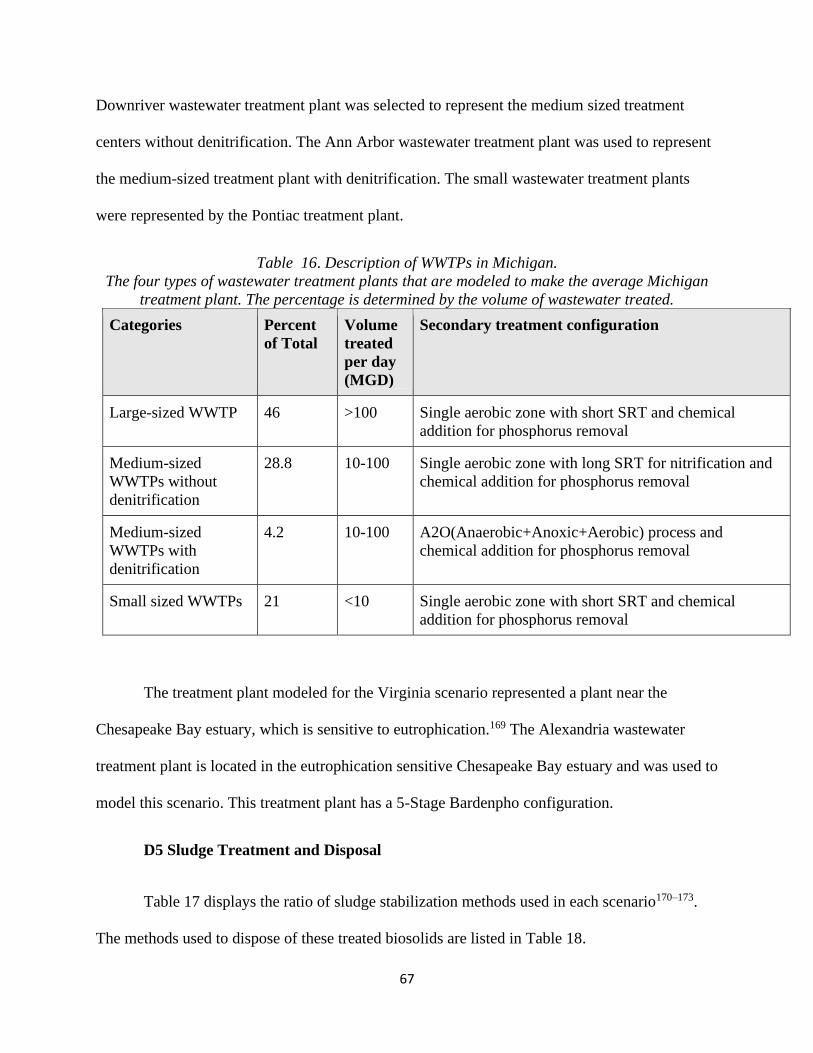
67
Downriver wastewater treatment plant was selected to represent the medium sized treatment
centers without denitrification. The Ann Arbor wastewater treatment plant was used to represent
the medium-sized treatment plant with denitrification. The small wastewater treatment plants
were represented by the Pontiac treatment plant.
Table 16. Description of WWTPs in Michigan.
The four types of wastewater treatment plants that are modeled to make the average Michigan
treatment plant. The percentage is determined by the volume of wastewater treated.
Categories Percent
of Total
Volume
treated
per day
(MGD)
Secondary treatment configuration
Large-sized WWTP 46 >100 Single aerobic zone with short SRT and chemical
addition for phosphorus removal
Medium-sized
WWTPs without
denitrification
28.8 10-100 Single aerobic zone with long SRT for nitrification and
chemical addition for phosphorus removal
Medium-sized
WWTPs with
denitrification
4.2 10-100 A2O(Anaerobic+Anoxic+Aerobic) process and
chemical addition for phosphorus removal
Small sized WWTPs 21 <10 Single aerobic zone with short SRT and chemical
addition for phosphorus removal
The treatment plant modeled for the Virginia scenario represented a plant near the
Chesapeake Bay estuary, which is sensitive to eutrophication.169 The Alexandria wastewater
treatment plant is located in the eutrophication sensitive Chesapeake Bay estuary and was used to
model this scenario. This treatment plant has a 5-Stage Bardenpho configuration.
D5 Sludge Treatment and Disposal
Table 17 displays the ratio of sludge stabilization methods used in each scenario170–173.
The methods used to dispose of these treated biosolids are listed in Table 18.

68
Table 17. Sludge Treatment Methods used in each Scenario.
*Due to a very low percent of aerobic digestion, this was included with anaerobic digestion.
Treatment Process Michigan Vermont Virginia
Anaerobic Digestion* 11% 23.7% 47.8%
Lime Stabilization 44.5% 42.9% 11.4%
Incineration 11.5% 1.6% 40.1%
Thermal Drying 33% 0% 0.667%
Compost 0% 31.8% 0%
Table 18. End of life for biosolids in each scenario.
Treatment Michiga
n Vermont Virginia
Land Applied (25%
solids) 23.5% 48.2% 28.7%
Land applied (90%
solids) 33.0% 0% 0.67%
Landfilled (25%
solids) 32.0% 50.2% 30.5%
Incinerated 11.5% 1.60% 40.1%
D6 Transportation Distances
Table 19 lists the distances required to transport urine derived fertilizers and activated
carbon for each scenario. Google Maps was used to determine the distance between the
wastewater treatment plant and the end location. The wastewater treatment plant was selected
because it was assumed that the urine derived fertilizer production plant was located near the
wastewater treatment plant. For urine derived fertilizers, the distance to the two closest large-
scale fertilizer distributors was quantified and averaged to account for the possibility that a
fertilizer distributor would not accept all of the fertilizer produced.

69
Table 19. Shipping distances in different scenarios.
All distances are in kilometers.
Material Vermont Michigan Virginia
Activated
Carbon 500 350 425
Fertilizer 28.4 17.7 63.2

70
APPENDIX E: SENSITIVITY ANALYSIS
Sensitivity analyses were used to assess the robustness of the results, to expand the
results beyond three specific cases, and to test the uncertainty due to the parameters and choices
selected for each scenario. Figure 6 shows the 12 simulation scenarios evaluated using a Monte
Carlo with 10,000 repetitions. The important parameters were determined using a one-at-a-time
sensitivity analysis. Some parameters that were correlated, such as TSS removal and BOD
removal during primary clarification, were then linked. Data on each parameter were collected in
order to determine a probability distribution. In cases where there were few data points or these
systems are only in early stages of development (e.g. urine collection systems), a conservative
approach was used and either triangular or uniform distributions were used. All distributions are
listed in Table 20, and some are discussed afterwards.
Figure 6. Depiction of simulations ran in sensitivity analysis.
Each of the 12 boxes at the bottom indicate an individual Monte Carlo with 10,000 repetitions.
StAS stands for Struvite and Ammonium Sulfate and Uconc stands for Urine Concentration.
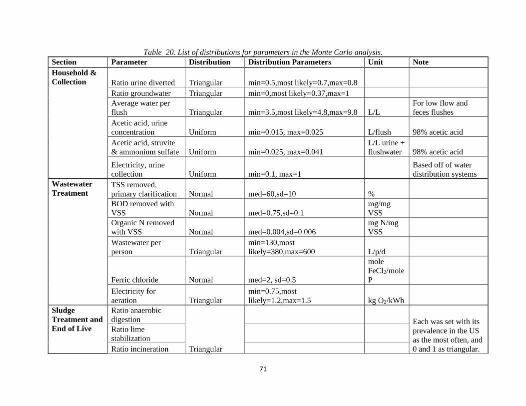
71
Table 20. List of distributions for parameters in the Monte Carlo analysis.
Section Parameter Distribution Distribution Parameters Unit Note
Household &
Collection Ratio urine diverted Triangular min=0.5,most likely=0.7,max=0.8
Ratio groundwater Triangular min=0,most likely=0.37,max=1
Average water per
flush Triangular min=3.5,most likely=4.8,max=9.8 L/L
For low flow and
feces flushes
Acetic acid, urine
concentration Uniform min=0.015, max=0.025 L/flush 98% acetic acid
Acetic acid, struvite
& ammonium sulfate Uniform min=0.025, max=0.041
L/L urine +
flushwater 98% acetic acid
Electricity, urine
collection Uniform min=0.1, max=1
Based off of water
distribution systems
Wastewater
Treatment TSS removed,
primary clarification Normal med=60,sd=10 %
BOD removed with
VSS Normal med=0.75,sd=0.1
mg/mg
VSS
Organic N removed
with VSS Normal med=0.004,sd=0.006
mg N/mg
VSS
Wastewater per
person Triangular
min=130,most
likely=380,max=600 L/p/d
Ferric chloride Normal med=2, sd=0.5
mole
FeCl2/mole
P
Electricity for
aeration Triangular
min=0.75,most
likely=1.2,max=1.5 kg O2/kWh
Sludge
Treatment and
End of Live
Ratio anaerobic
digestion
Triangular
Each was set with its
prevalence in the US
as the most often, and
0 and 1 as triangular.
Ratio lime
stabilization
Ratio incineration

72
Ratio drying These were scaled to
equal 1.174 Ratio composting
Land applied, 25%
solid
Triangular
Ratio of these two
types of sludge
treatment. Max=ratio
of land applied-
thermally dried to
ratio landfilled. Other
end of life determined
by treatment
method.174 Landfilled
Struvite &
Ammonium
Sulfate
Struvite P recovery
ratio Triangular
min=0.9,most
likely=0.96,max=0.99
Ion exchange N
recovery Uniform min=0.93,max=0.99
Ion exchange
stoichiometric ratio Triangular
min=0.71,most
likely=0.91,max=0.98
1 indicates every
mole of sulfate binds
with ammonium.
Performance often
increases as systems
continue to be
developed. Weak
Acid Cation
Exchange systems
often said to operate
near 100% efficiency.
Urine
Concentration Uconc N recovery Uniform min=0.91,max=0.99
Uconc P recovery Uniform min=0.98,max=1
Uconc COD recovery Uniform min=0.95,max=0.99

73
Uconc electricity
consumption Triangular Beta
min=0.002,most
likely=0.0035,max=0.036
kWh/L
permeate
removed
Based off of small
scale desalination
reverse osmosis
systems with Energy
Recovery Devices.
Fertilizer
Transportation Ratio synthetic
fertilizer sent by
truck Triangular
min=0.015,most
likely=0.78,max=0.22,shape=6
Remaining trip 2/3 on
rail, 1/3 on barge.
From different
fertilizer types.175
Distance UD is
shipped
Truncated
lognormal median=85,sd=75,min=5,max=500 km
Determined from
Google Maps
searches,176 Trimmer
and Guest,100 and US
city size statistics. All
via truck.

74
Ion exchange stoichiometric ratio
The amount of sulfuric acid used to regenerate ion exchange resin was one of the most
important parameters for the struvite and ammonium sulfate alternative. The stoichiometric ratio
is how many ions of sulfuric acid are needed relative to the amount of ammonium ions removed.
A weak acid cation exchange resin is used, which are said to often operate near 100% efficiency.
The data used in the study are from small-scale experiments, and have a much lower efficiency.
The triangular distribution selected assumes that efficiency will improve as the practice becomes
more common.
Urine concentration electricity
The electricity demand from reverse osmosis was one of the most important parameters
for the urine concentration alternative. The study used a small-scale system for electricity
consumption. The Monte Carlo evaluated small-scale desalination systems with energy recovery
devices to evaluate how energy intensive reverse osmosis may be at this scale. Desalination was
selected as a proxy because much data are available and ocean water has a higher total dissolved
solids than urine.
Distance urine is shipped
The probability distribution for distances urine is shipped were estimated by the amount
of people in certain sized cities and relevant distances for each. Distances in cities with less than
500,000 were estimated using Google Maps searches. Distances found in Trimmer and Guest100
were used to estimate distances from larger cities. All transportation was assumed to be via
truck, though it is certainly possible that larger cities could use trains.

75
APPENDIX F: SUPPLEMENTAL RESULTS
More information on the results are shown below. The first section contains graphs
comparing the three alternatives in Vermont (Figure 7) and Michigan (Figure 8). The next
section has graphs showing each impact measured per component in all scenarios and
alternatives (Figures 9-22). Figure 23 then compares different methodologies for estimating the
changes in wastewater treatment due to urine diversion.
F1 Comparison of Alternatives
Figure 7. Normalized Impacts in Vermont Scenario.
Total impacts in each alternative normalized to the maximum value.
0%
10%
20%
30%
40%
50%
60%
70%
80%
90%
100%
GWP CED Water EP AP
Per
cen
t o
f M
axim
um
Impact Category
Urine Concentration Struvite and Ammonium Sulfate Conventional

76
Figure 8. Normalized Impacts in Michigan Scenario.
Total impacts in each alternative normalized to the maximum value.
F2 Impacts per Component
Figure 9. GWP of the Vermont alternatives by Process.
0%
10%
20%
30%
40%
50%
60%
70%
80%
90%
100%
GWP CED Water EP AP
Per
cen
t o
f M
axim
um
Impact Catgeory
Urine Concentration Struvite and Ammonium Sulfate Conventional
0
5
10
15
20
25
30
Urine Concentration Struvite and AmmoniumSulfate
Conventional
kg C
O2e
/ca
pit
a۰ye
ar
VermontGlobal Warming Potential
Others Synthetic fertilizerTransport UDF Production-ChemicalsUDF Production-Electricity Urine CollectionSecondary Sludge Treatment Wastewater Treatment (excluding sludge)Water Production

77
Figure 10. CED of the Vermont alternatives by Process.
Figure 11. Freshwater use of the Vermont alternatives by Process.
0
50
100
150
200
250
300
350
400
450
500
Urine Concentration Struvite and AmmoniumSulfate
Conventional
MJ/
cap
ita۰
year
VermontCumulative Energy Demand
Others Synthetic fertilizer
Transport UDF Production-Chemicals
UDF Production-Electricity Urine Collection
Secondary Sludge Treatment Wastewater Treatment (excluding sludge)
Water Production
0
2
4
6
8
10
12
14
16
Urine Concentration Struvite and AmmoniumSulfate
Conventional
m3 /
cap
ita۰
year
VermontFreshwater Use
Others Synthetic fertilizer
Transport UDF Production-Chemicals
UDF Production-Electricity Urine Collection
Secondary Sludge Treatment Wastewater Treatment (excluding sludge)
Water Production

78
Figure 12. Eutrophication potential of the Vermont alternatives by Process.
Figure 13. Acidification potential of the Vermont alternatives by Process.
0
0.5
1
1.5
2
2.5
3
3.5
Urine Concentration Struvite and AmmoniumSulfate
Conventional
kg N
e/ca
pit
a۰ye
ar
VermontEutrophication Potential
Others Synthetic fertilizerTransport UDF Production-ChemicalsUDF Production-Electricity Urine CollectionSecondary Sludge Treatment Wastewater Treatment (excluding sludge)Water Production
0
0.02
0.04
0.06
0.08
0.1
0.12
Urine Concentration Struvite and AmmoniumSulfate
Conventional
kg S
Oxe
/cap
ita۰
year
VermontAcidification Potential
Others Synthetic fertilizerTransport UDF Production-ChemicalsUDF Production-Electricity Urine CollectionSecondary Sludge Treatment Wastewater Treatment (excluding sludge)Water Production
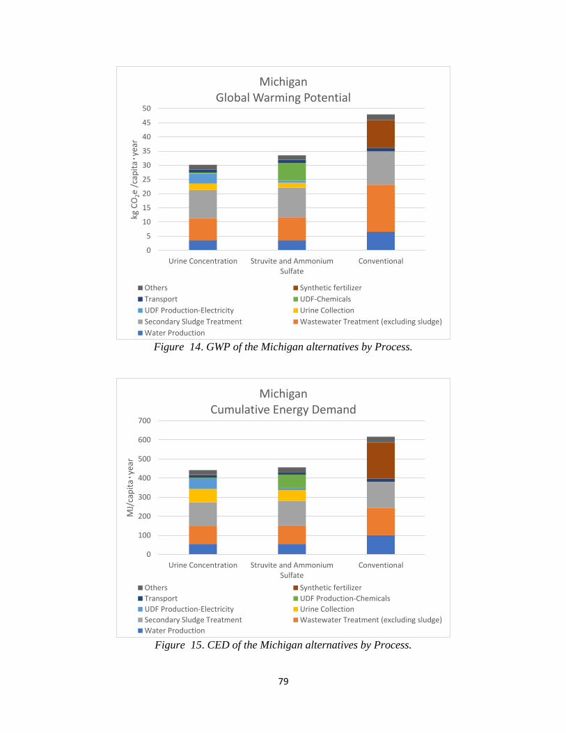
79
Figure 14. GWP of the Michigan alternatives by Process.
Figure 15. CED of the Michigan alternatives by Process.
0
5
10
15
20
25
30
35
40
45
50
Urine Concentration Struvite and AmmoniumSulfate
Conventional
kg C
O2e
/ca
pit
a۰ye
ar
MichiganGlobal Warming Potential
Others Synthetic fertilizer
Transport UDF-Chemicals
UDF Production-Electricity Urine Collection
Secondary Sludge Treatment Wastewater Treatment (excluding sludge)
Water Production
0
100
200
300
400
500
600
700
Urine Concentration Struvite and AmmoniumSulfate
Conventional
MJ/
cap
ita۰
year
MichiganCumulative Energy Demand
Others Synthetic fertilizer
Transport UDF Production-Chemicals
UDF Production-Electricity Urine Collection
Secondary Sludge Treatment Wastewater Treatment (excluding sludge)
Water Production

80
Figure 16. Freshwater use of the Michigan alternatives by Process.
0
2
4
6
8
10
12
14
16
Urine Concentration Struvite and AmmoniumSulfate
Conventional
m3/c
apit
a۰ye
ar
MichiganFreshwater Use
Others Synthetic fertilizer
Transport UDF-Chemicals
UDF Production-Electricity Urine Collection
Secondary Sludge Treatment Wastewater Treatment (excluding sludge)
Water Production
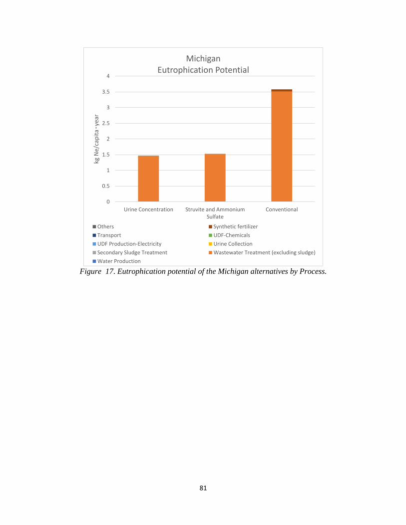
81
Figure 17. Eutrophication potential of the Michigan alternatives by Process.
0
0.5
1
1.5
2
2.5
3
3.5
4
Urine Concentration Struvite and AmmoniumSulfate
Conventional
kg N
e/ca
pit
a۰ye
ar
MichiganEutrophication Potential
Others Synthetic fertilizer
Transport UDF-Chemicals
UDF Production-Electricity Urine Collection
Secondary Sludge Treatment Wastewater Treatment (excluding sludge)
Water Production

82
Figure 18. Acidification potential of the Virginia alternatives by Process.
Figure 19. CED of the Virginia alternatives by Process.
0
0.02
0.04
0.06
0.08
0.1
0.12
0.14
0.16
0.18
0.2
Urine Concentration Struvite and AmmoniumSulfate
Conventional
kg S
Oxe
/cap
ita۰
year
MichiganAcidification Potential
Others Synthetic fertilizer
Transport UDF-Chemicals
UDF Production-Electricity Urine Collection
Secondary Sludge Treatment Wastewater Treatment (excluding sludge)
Water Production
0
100
200
300
400
500
600
700
Urine Concentration Struvite and AmmoniumSulfate
Conventional
MJ/
cap
ita۰
year
VirginiaCumulative Energy Demand
Others Synthetic fertilizer
Transport UDF Production-Chemicals
UDF Production-Electricity Urine Collection
Secondary Sludge Treatment Wastewater Treatment (excluding sludge)
Water Production

83
Figure 20. Freshwater use of the Virginia alternatives by Process.
Figure 21. Eutrophication potential of the Virginia alternatives by Process.
0
2
4
6
8
10
12
14
Urine Concentration Struvite and AmmoniumSulfate
Conventional
m3 /
cap
ita۰
year
VirginiaFreshwater Use
Others Synthetic fertilizer
Transport UDF Production-Chemicals
UDF Production-Electricity Urine Collection
Secondary Sludge Treatment Wastewater Treatment (excluding sludge)
Water Production
0
0.05
0.1
0.15
0.2
0.25
0.3
0.35
0.4
0.45
Urine Concentration Struvite and AmmoniumSulfate
Conventional
kg N
e/ca
pit
a۰ye
ar
VirginiaEutrophication Potential
Others Synthetic fertilizerTransport UDF Production-ChemicalsUDF Production-Electricity Urine CollectionSecondary Sludge Treatment Wastewater Treatment (excluding sludge)Water Production
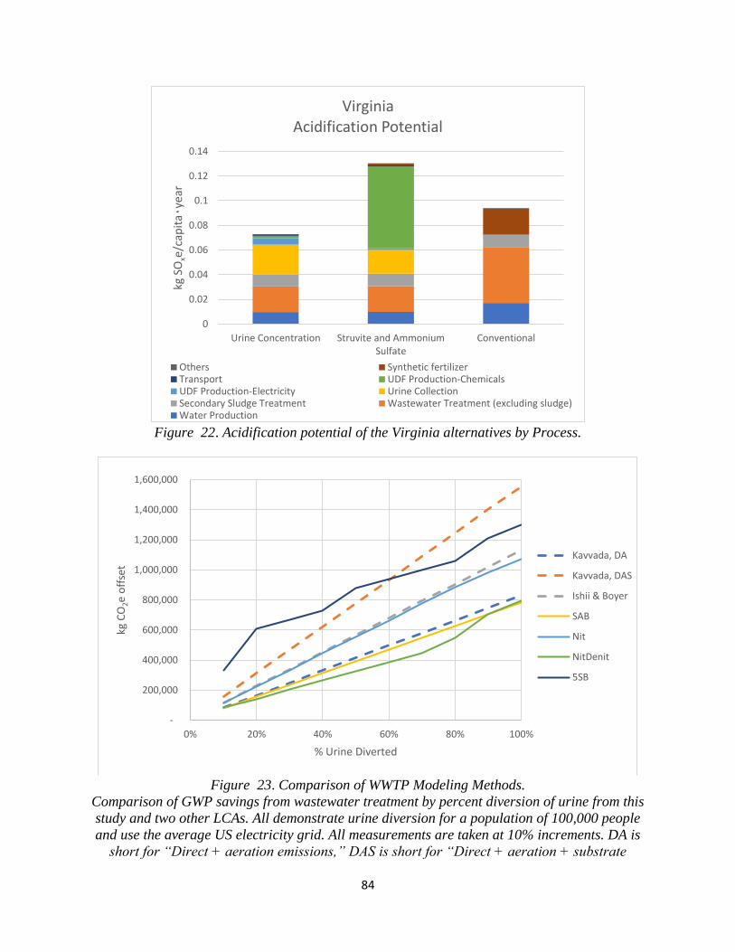
84
Figure 22. Acidification potential of the Virginia alternatives by Process.
Figure 23. Comparison of WWTP Modeling Methods.
Comparison of GWP savings from wastewater treatment by percent diversion of urine from this
study and two other LCAs. All demonstrate urine diversion for a population of 100,000 people
and use the average US electricity grid. All measurements are taken at 10% increments. DA is
short for “Direct + aeration emissions,” DAS is short for “Direct + aeration + substrate
0
0.02
0.04
0.06
0.08
0.1
0.12
0.14
Urine Concentration Struvite and AmmoniumSulfate
Conventional
kg S
Oxe
/cap
ita۰
year
VirginiaAcidification Potential
Others Synthetic fertilizerTransport UDF Production-ChemicalsUDF Production-Electricity Urine CollectionSecondary Sludge Treatment Wastewater Treatment (excluding sludge)Water Production
-
200,000
400,000
600,000
800,000
1,000,000
1,200,000
1,400,000
1,600,000
0% 20% 40% 60% 80% 100%
kg C
O2e
off
set
% Urine Diverted
Kavvada, DA
Kavvada, DAS
Ishii & Boyer
SAB
Nit
NitDenit
5SB

85
emissions,” SAB is short for “Single Aeration Basin,” Nit is short for “Nitrification,” NitDenit is
short for “Nitrification and Denitrification,” and 5SB is short for “5-Stage Bardenpho.”
The simpler methods used in other studies to estimate how much urine diversion reduces
the greenhouse gas emissions associated with wastewater treatment produce relatively similar
results.48,49 Using a denitrification emission factor without substrate emissions can be a close
approximation for less stringent treatment plants, even though some do not actually use
denitrification.49 Using a denitrification emission factor with substrate emissions leads to results
relatively close to the stringent 5-Stage Bardenpho treatment plant modeled in this study.
Offsetting by volume of wastewater treatment can produce relatively similar results, though it is
worth noting that the wastewater treatment plant in Ishii and Boyer’s study consumes more
electricity per cubic meter of wastewater than most.48,59 This volumetric approach may
underestimate actual savings when the electricity grid uses a large proportion of renewable
energy sources, a urine diverting toilet’s flush volume is not much lower than the alternative, or
when the wastewater treatment plant does not consume an above average amount of electricity
per volume wastewater.
Most treatment plants did not have constant improvements as the level of urine diversion
increased. Whenever the need for a chemical input is eliminated, increases to urine diversion past
that point lead to smaller environmental gains. At certain levels of urine diversion, the treatment
configuration of the treatment plant could be simplified, leading to relatively large environmental
benefits. Using simplified methods to estimate changes to wastewater treatment will not capture
these complexities. They are useful as a reasonable approximation of environmental benefits.
The methods in this study would be useful for a more accurate approximation, for a clearer idea

86
of how operations will change (e.g. typically will not need external carbon sources), or
comparing the merits and drawbacks of different levels of urine diversion.
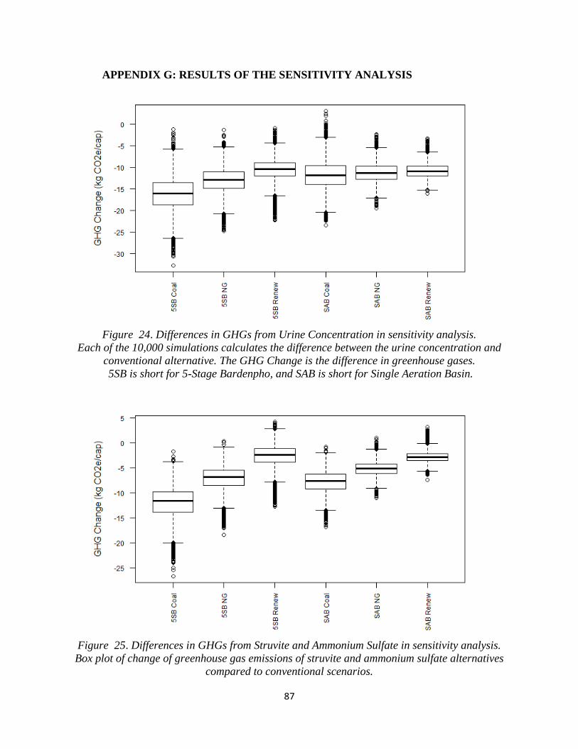
87
APPENDIX G: RESULTS OF THE SENSITIVITY ANALYSIS
Figure 24. Differences in GHGs from Urine Concentration in sensitivity analysis.
Each of the 10,000 simulations calculates the difference between the urine concentration and
conventional alternative. The GHG Change is the difference in greenhouse gases.
5SB is short for 5-Stage Bardenpho, and SAB is short for Single Aeration Basin.
Figure 25. Differences in GHGs from Struvite and Ammonium Sulfate in sensitivity analysis.
Box plot of change of greenhouse gas emissions of struvite and ammonium sulfate alternatives
compared to conventional scenarios.
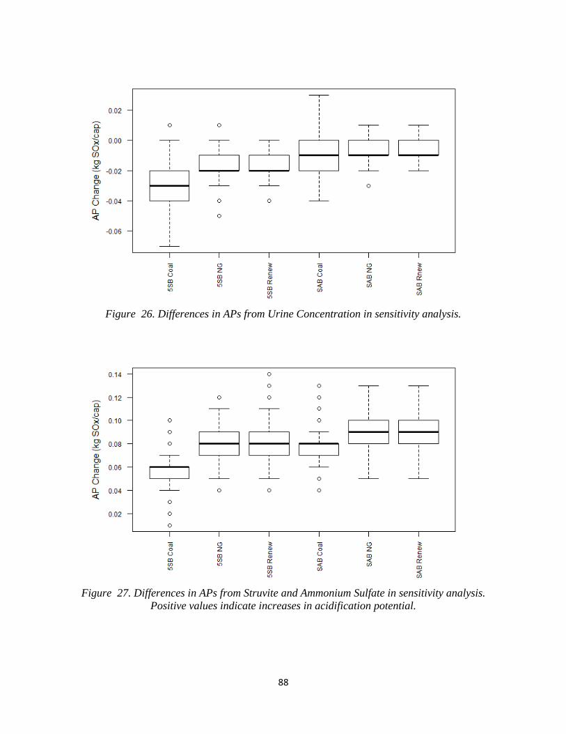
88
Figure 26. Differences in APs from Urine Concentration in sensitivity analysis.
Figure 27. Differences in APs from Struvite and Ammonium Sulfate in sensitivity analysis.
Positive values indicate increases in acidification potential.
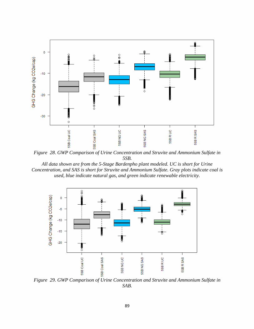
89
Figure 28. GWP Comparison of Urine Concentration and Struvite and Ammonium Sulfate in
5SB.
All data shown are from the 5-Stage Bardenpho plant modeled. UC is short for Urine
Concentration, and SAS is short for Struvite and Ammonium Sulfate. Gray plots indicate coal is
used, blue indicate natural gas, and green indicate renewable electricity.
Figure 29. GWP Comparison of Urine Concentration and Struvite and Ammonium Sulfate in
SAB.

90
All data shown are from the single aeration basin plant modeled. UC is short for Urine
Concentration, and SAS is short for Struvite and Ammonium Sulfate. Gray plots indicate coal is
used, blue indicate natural gas, and green indicate renewable electricity.
Table 21. Urine Concentration Scenarios with lower GWP.
Percent of simulations where urine concentration had lower greenhouse gas emissions than the
conventional alternative with different scopes. The first row is what was measured in the study,
the second row is if fertilizer offsets were not considered, and the third row is if N2O emissions
from effluent were not considered.
Urine Concentration
5SB
Coal
5SB
NG 5SB Renew
SAB
Coal
SAB
NG SAB Renew
Standard 100.0% 99.9% 100.0% 100.0% 100.0% 100.0%
W/o fert offset 97.5% 94.5% 77.2% 82.6% 88.7% 92.7%
W/o external N2O 100.0% 100.0% 100.0% 99.3% 100.0% 1.0%
Table 22. Struvite and Ammonium Sulfate Scenarios with lower GWP.
Percent of simulations where struvite and ammonium sulfate had lower greenhouse gas
emissions than the conventional alternative with different scopes. The first row is what was
measured in the study, the second row is if fertilizer offsets were not considered, and the third
row is if N2O emissions from effluent were not considered.
Struvite and Ammonium Sulfate
5SB Coal
5SB
NG 5SB Renew
SAB
Coal
SAB
NG SAB Renew
Standard 100.0% 100.0% 91.7% 100.0% 99.9% 98.7%
W/o fert offset 85.9% 19.8% 2.6% 27.7% 0.2% 0.0%
W/o external N2O 100.0% 100.0% 91.4% 99.4% 93.8% 0.4%

91
REFERENCES
1. Stewart, W. M., Dibb, D. W., Johnston, A. E. & Smyth, T. J. The contribution of
commercial fertilizer nutrients to food production. Agron. J. 97, 1–6 (2005).
2. Scholz, R. W. & Wellmer, F.-W. Although there is no Physical Short-Term Scarcity of
Phosphorus, its Resource Efficiency Should be Improved. J. Ind. Ecol. (2018).
doi:10.1111/jiec.12750
3. Cordell, D. & White, S. Peak phosphorus: Clarifying the key issues of a vigorous debate
about long-term phosphorus security. Sustainability 3, 2027–2049 (2011).
4. Cordell, D., Drangert, J.-O. & White, S. The story of phosphorus: Global food security
and food for thought. Glob. Environ. Chang. 19, 292–305 (2009).
5. Chen, M. & Graedel, T. E. A half-century of global phosphorus flows, stocks, production,
consumption, recycling, and environmental impacts. Glob. Environ. Chang. 36, 139–152
(2016).
6. Dawson, C. J. & Hilton, J. Fertiliser availability in a resource-limited world: Production
and recycling of nitrogen and phosphorus. Food Policy 36, (2011).
7. Wood, Sam; Cowie, A. A Review of Greenhouse Gas Emissions for Fertiliser Production.
Coop. Res. Cent. Greenh. Account. 20 (2004).
8. Jacobs, B., Cordell, D., Chin, J. & Rowe, H. Towards phosphorus sustainability in North
America: A model for transformational change. Environ. Sci. Policy 77, 151–159 (2017).
9. Elliot, T. Energy-Saving Opportunities for Wastewater Facilities: A Review. Energy Cent.
Wisconsin 221–1, (2003).

92
10. U.S. EPA. State and Local Climate and Energy Program: Water/Wastewater. (2012).
Available at: https://www.epa.gov/statelocalenergy.
11. Guest, J. S. et al. A new planning and design paradigm to achieve sustainable resource
recovery from wastewater. Environ. Sci. Technol. 43, 6126–6130 (2009).
12. Roy, E. D. Phosphorus recovery and recycling with ecological engineering: A review.
Ecol. Eng. 98, 213–227 (2017).
13. Lam, L., Kurisu, K. & Hanaki, K. Comparative environmental impacts of source-
separation systems for domestic wastewater management in rural China. J. Clean. Prod.
104, 185–198 (2015).
14. Lundin, M., Bengtsson, M. & Molander, S. Life cycle assessment of wastewater systems:
Influence of system boundaries and scale on calculated environmental loads. Environ. Sci.
Technol. 34, 180–186 (2000).
15. Maurer, M., Pronk, W. & Larsen, T. A. Treatment processes for source-separated urine.
Water Res. 40, 3151–3166 (2006).
16. Slagstad, H. & Brattebø, H. Life cycle assessment of the water and wastewater system in
Trondheim, Norway - A case study: Case Study. Urban Water J. 11, 323–334 (2014).
17. Pasqualino, J. C., Meneses, M., Abella, M. & Castells, F. LCA as a decision support tool
for the environmental improvement of the operation of a municipal wastewater treatment
plant. Environ. Sci. Technol. 43, 3300–3307 (2009).
18. Wilsenach, J. & Van Loosdrecht, M. Impact of separate urine collection on wastewater
treatment systems. Water Science and Technology 48, (2003).

93
19. Simha, P. & Ganesapillai, M. Ecological Sanitation and nutrient recovery from human
urine: How far have we come? A review. Sustain. Environ. Res. 27, 107–116 (2017).
20. Johnston, A. E. & Richards, I. R. Effectiveness of different precipitated phosphates as
phosphorus sources for plants. Soil Use Manag. 19, 45–49 (2003).
21. Ricardo, G.-P., López-de-Sá, E. G. & Plaza, C. Lettuce response to phosphorus
fertilization with struvite recovered from municipal wastewater. HortScience 44, 426–430
(2009).
22. Skowronska, M. & Filipek, T. Life cycle assessment of fertilizers: a review. Int.
Agrophysics 28, 101–110 (2014).
23. Sloan, J. J., Dowdy, R. H., Dolan, M. S. & Linden, D. R. Long-term effects of biosolids
applications on heavy metal bioavailability in agricultural soils. J. Environ. Qual. 26,
966–974 (1997).
24. Jönsson, H., Stenström, T.-A., Svensson, J. & Sundin, A. Source separated urine-nutrient
and heavy metal content, water saving and faecal contamination. Water Science and
Technology 35, (1997).
25. Wigginton, K. R. et al. Nutrient Recovery Through Urine Separation. (2017).
26. Diaz-Elsayed, N., Rezaei, N., Guo, T., Mohebbi, S. & Zhang, Q. Wastewater-based
resource recovery technologies across scale: A review. Resour. Conserv. Recycl. 145, 94–
112 (2019).
27. Udert, K. M., Larsen, T. A., Biebow, M. & Gujer, W. Urea hydrolysis and precipitation
dynamics in a urine-collecting system. Water Res. 37, 2571–2582 (2003).

94
28. Ray, H., Saetta, D. & Boyer, T. H. Characterization of urea hydrolysis in fresh human
urine and inhibition by chemical addition. Environ. Sci. Water Res. Technol. 4, 87–98
(2018).
29. Saetta, D. & Boyer, T. H. Mimicking and Inhibiting Urea Hydrolysis in Nonwater Urinals.
Environ. Sci. Technol. 51, 13850–13858 (2017).
30. Thörneby, L., Persson, K. & Trägårdh, G. Treatment of liquid effluents from dairy cattle
and pigs using reverse osmosis. J. Agric. Eng. Res. 73, 159–170 (1999).
31. Tian, X. et al. Reverse osmosis brine for phosphorus recovery from source separated
urine. Chemosphere 165, 202–210 (2016).
32. Lorain, O., Thiebaud, P., Badorc, E. & Aurelle, Y. Potential of freezing in wastewater
treatment: Soluble pollutant applications. Water Res. 35, 541–547 (2001).
33. Gulyas, H. et al. Freeze concentration for enrichment of nutrients in yellow water from
no-mix toilets. Water Science and Technology 50, (2004).
34. Lind, B.-B., Ban, Z. & Bydén, S. Volume reduction and concentration of nutrients in
human urine. Ecol. Eng. 16, 561–566 (2001).
35. Bridger, G. L., Salutsky, M. L. & Starostka, R. W. Micronutrient Sources, Metal
Ammonium Phosphates as Fertilizers. J. Agric. Food Chem. 10, 181–188 (1962).
36. Ganrot, Z., Dave, G. & Nilsson, E. Recovery of N and P from human urine by freezing,
struvite precipitation and adsorption to zeolite and active carbon. Bioresour. Technol. 98,
3112–3121 (2007).
37. Doyle, J. D. & Parsons, S. A. Struvite formation, control and recovery. Water Res. 36,

95
3925–3940 (2002).
38. Schuiling, R. D. & Andrade, A. Recovery of struvite from calf manure. Environ. Technol.
(United Kingdom) 20, 765–768 (1999).
39. Tarpeh, W. A., Udert, K. M. & Nelson, K. L. Comparing ion exchange adsorbents for
nitrogen recovery from source-separated urine. Environ. Sci. Technol. 51, 2373–2381
(2017).
40. Ganesapillai, M., Simha, P. & Zabaniotou, A. Closed-loop fertility cycle: Realizing
sustainability in sanitation and agricultural production through the design and
implementation of nutrient recovery systems for human urine. Sustain. Prod. Consum. 4,
36–46 (2015).
41. Udert, K. M. & Wächter, M. Complete nutrient recovery from source-separated urine by
nitrification and distillation. Water Res. 46, 453–464 (2012).
42. International Standards Organization (ISO). International Standard 14040: Life Cycle
Assessment-Principles and Framework. (2006).
43. International Standards Organization (ISO). ISO 14044: Life Cycle Assessment -
Principles and Framework. (2006).
44. Arpke, A. & Hutzler, N. Domestic water use in the United States: A life-cycle approach.
J. Ind. Ecol. 10, 169–184 (2006).
45. Rahman, S. M., Eckelman, M. J., Onnis-Hayden, A. & Gu, A. Z. Life-Cycle Assessment
of Advanced Nutrient Removal Technologies for Wastewater Treatment. Environ. Sci.
Technol. 50, 3020–3030 (2016).

96
46. Corominas, L. et al. Life cycle assessment applied to wastewater treatment: State of the
art. Water Res. 47, 5480–5492 (2013).
47. Risch, E., Gutierrez, O., Roux, P., Boutin, C. & Corominas, L. Life cycle assessment of
urban wastewater systems: Quantifying the relative contribution of sewer systems. Water
Res. 77, 35–48 (2015).
48. Ishii, S. K. L. & Boyer, T. H. Life cycle comparison of centralized wastewater treatment
and urine source separation with struvite precipitation: Focus on urine nutrient
management. Water Res. 79, 88–103 (2015).
49. Kavvada, O., Tarpeh, W. A., Horvath, A. & Nelson, K. L. Life-cycle cost and
environmental assessment of decentralized nitrogen recovery using ion exchange from
source-separated urine through spatial modeling. Environ. Sci. Technol. 51, 12061–12071
(2017).
50. Remy, C. & Jekel, M. Energy analysis of conventional and source-separation systems for
urban wastewater management using Life Cycle Assessment. Water Sci. Technol. 65, 22–
29 (2012).
51. Xue, X., Hawkins, T. R., Schoen, M. E., Garland, J. & Ashbolt, N. J. Comparing the life
cycle energy consumption, globalwarming and eutrophication potentials of several water
and waste service options. Water (Switzerland) 8, (2016).
52. Jimenez, J., Bott, C., Love, N. & Bratby, J. Source Separation of Urine as an Alternative
Solution to Nutrient Management in Biological Nutrient Removal Treatment Plants.
Water Environ. Res. 87, 2120–2129 (2015).
97
53. Ekama, G. A., Wilsenach, J. A. & Chen, G. H. Saline sewage treatment and source
separation of urine for more sustainable urban water management. Water Sci. Technol. 64,
1307–1316 (2011).
54. Wilsenach, J. A., Schuurbiers, C. A. H. & van Loosdrecht, M. C. M. Phosphate and
potassium recovery from source separated urine through struvite precipitation. Water Res.
41, 458–466 (2007).
55. Maupin, M. et al. Estimated Use of Water in the United States in 2010. U.S. Geol. Surv.
Circ. 56 (2014).
56. Bonton, A., Bouchard, C., Barbeau, B. & Jedrzejak, S. Comparative life cycle assessment
of water treatment plants. Desalination 284, 42–54 (2012).
57. D&R International, L. 2011 Buildings Energy Data Book. (U.S. Department of Energy,
2012).
58. Elliot, T., Zeier, B., Xagoraraki, I. & Harrington, G. Energy Use at Wisconsin’s Drinking
Water Utilities. (2002).
59. EPRI. Water & Sustainability (Volume 4): U.S. Electricity Consumption for Water Supply
& Treatment - The Next Half Century. (2002).
60. Godskesen, B., Hauschild, M., Rygaard, M., Zambrano, K. & Albrechtsen, H.-J. Life
cycle assessment of central softening of very hard drinking water. J. Environ. Manage.
105, 83–89 (2012).
61. Jeong, H., Minne, E. & Crittenden, J. C. Life cycle assessment of the City of Atlanta,
Georgia’s centralized water system. Int. J. Life Cycle Assess. 20, 880–891 (2015).

98
62. Kjellsson, J. B., Greene, D., Bhattarai, R. & Webber, M. E. Energy benchmarking of
water and wastewater treatment, distribution and collection: A case study of Austin water
utility. in ASME International Mechanical Engineering Congress and Exposition,
Proceedings (IMECE) 6 B, (2013).
63. Mo, W., Nasiri, F., Eckelman, M. J., Zhang, Q. & Zimmerman, J. B. Measuring the
embodied energy in drinking water supply systems: A case study in the Great Lakes
region. Environ. Sci. Technol. 44, 9516–9521 (2010).
64. Renzoni, R. & Germain, A. Life Cycle Assessment of Water from the Pumping Station to
the Wastewater Treatment Plant. Int J Life Cycle Assess. 12, 118 (2007).
65. Stokes, J. R. & Horvath, A. Energy and air emission effects of water supply. Environ. Sci.
Technol. 43, 2680–2687 (2009).
66. Tripathi, M. Life-Cycle Energy and Emissions for Municipal Water and Wastewater
Services: Case-Studies of Treatment Plants in US. (University of Michigan, 2007).
67. Plappally, A. K. & Lienhard V, J. H. Energy requirements for water production, treatment,
end use, reclamation, and disposal. Renew. Sustain. Energy Rev. 16, 4818–4848 (2012).
68. CABOT. Norit PK 3-5. (2018).
69. Bayer, P., Heuer, E., Karl, U. & Finkel, M. Economical and ecological comparison of
granular activated carbon (GAC) adsorber refill strategies. Water Res. 39, 1719–1728
(2005).
70. He, K. A calculation of the environmental footprint of a granular activated carbon
regeneration facility. Clim. Energy Sect. Environ. Sci. Sr. Thesis Symp. UC Berkeley

99
Environ. Sci. 22, 28 (2012).
71. Hutchins, R. A. Thermal Regeneration Costs. Chem. Eng. Prog. 71, 80–86 (1975).
72. Meier, M. Eco-efficiency evaluation of waste gas purification systems in the chemical
industry. (ETH Zurich, 1997).
73. Hydranautics. Foulants and Cleaning Procedures for composite polyamide RO Membrane
Elements (ESP, ESNA, CPA, LFC, NANO and SWC). Technical Service Bulletin 16
(2014). Available at: http://www.membranes.com/docs/tsb/TSB107.pdf. (Accessed: 3rd
July 2018)
74. Hilton, S. et al. Life Cycle Assessment of Urine Diversion Wastewater Treatment: Results
and Software Tool. (2018).
75. Antonini, S., Arias, M. A., Eichert, T. & Clemens, J. Greenhouse evaluation and
environmental impact assessment of different urine-derived struvite fertilizers as
phosphorus sources for plants. Chemosphere 89, 1202–1210 (2012).
76. Achat, D. L. et al. Plant-availability of phosphorus recycled from pig manures and dairy
effluents as assessed by isotopic labeling techniques. Geoderma 232, 24–33 (2014).
77. Germer, J., Addai, S. & Sauerborn, J. Response of grain sorghum to fertilisation with
human urine. F. Crop. Res. 122, 234–241 (2011).
78. Zhang, Z. & Wilson, F. Life-cycle assessment of a sewage-treatment plant in south-east
asia. Water Environ. J. 14, 51–56 (2000).
79. Piratla, K. R., Ariaratnam, S. T. & Cohen, A. Estimation of CO <inf>2</inf> emissions
from the life cycle of a potable water pipeline project. J. Manag. Eng. 28, 22–30 (2012).
100
80. Lundie, S., Peters, G. M. & Beavis, P. C. Life cycle assessment for sustainable
metropolitan water systems planning. Environ. Sci. Technol. 38, 3465–3473 (2004).
81. EMMERSON, R. H. C., MORSE, G. K., LESTER, J. N. & EDGE, D. R. The Life‐Cycle
Analysis of Small‐Scale Sewage‐Treatment Processes. Water and Environment Journal,
9(3), 317–325. https://doi.org/10.1111/j.1747. Water Environ. J. 9, 317–325 (1995).
82. National Renewable Energy Laboratory. U.S. Life Cycle Inventory Database. (2012).
83. ecoinvent. ecoinvent 3.4. (2017). Available at: https://www.ecoinvent.org/.
84. Koehler, A. Water use in LCA: Managing the planet’s freshwater resources. Int. J. Life
Cycle Assess. 13, 451–455 (2008).
85. WRF. Residential End Uses of Water, Version 2. (2016).
86. FitzGerald, M. P., Stablein, U. & Brubaker, L. Urinary habits among asymptomatic
women. Am. J. Obstet. Gynecol. 187, 1384–1388 (2002).
87. Friedler, E., Butler, D. & Brown, D. M. Domestic WC usage patterns. Build. Environ. 31,
385–392 (1996).
88. Vickers, A. Handbook of Water Use and Conservation. (Waterplow Press, 2001).
89. Burgio, K. L., Engel, B. T. & Locher, J. L. Normative patterns of diurnal urination across
6 age decades. J. Urol. 145, 728–731 (1991).
90. Sanjoaquin, M. A., Appleby, P. N., Spencer, E. A. & Key, T. J. Nutrition and lifestyle in
relation to bowel movement frequency: A cross-sectional study of 20 630 men and women
in EPIC-Oxford. Public Health Nutr. 7, 77–83 (2004).

101
91. Abegglen, C. K. Membrane bioreactor technology for decentralized wastewater treatment
and reuse. (ETH Zurich, 2008).
92. Antonini, S., Paris, S., Eichert, T. & Clemens, J. Nitrogen and Phosphorus Recovery from
Human Urine by Struvite Precipitation and Air Stripping in Vietnam. Clean - Soil, Air,
Water 39, 1099–1104 (2011).
93. Dastur, M. Investigation into the factors affecting controlled struvite crystallization at the
bench-scale. (University of British Columbia, 2001).
94. Ronteltap, M., Maurer, M., Hausherr, R. & Gujer, W. Struvite precipitation from urine –
Influencing factors on particle size. Water Res. 44, 2038–2046 (2010).
95. Grundestam, J. & Hellström, D. Wastewater treatment with anaerobic membrane
bioreactor and reverse osmosis. Water Science and Technology 56, (2007).
96. Ledda, C., Schievano, A., Salati, S. & Adani, F. Nitrogen and water recovery from animal
slurries by a new integrated ultrafiltration, reverse osmosis and cold stripping process: A
case study. Water Res. 47, 6157–6166 (2013).
97. Middleton, M. SimVoi Monte Carlo Simulation Add-In. (2016).
98. Ganrot, Z., Dave, G. & Nilsson, E. Recovery of N and P from human urine by freezing,
struvite precipitation and adsorption to zeolite and active carbon. Bioresour. Technol. 98,
3112–3121 (2007).
99. USDA. Fertilizer Use and Price. (2016).
100. Trimmer, J. T. & Guest, J. S. Recirculation of human-derived nutrients from cities to
agriculture across six continents. Nat. Sustain. 1, 427–435 (2018).

102
101. Metson, G. S., Bennett, E. M. & Elser, J. J. The role of diet in phosphorus demand.
Environ. Res. Lett. 7, (2012).
102. Ibarrola-Rivas, M. J. & Nonhebel, S. Variations in the use of resources for food: Land,
nitrogen fertilizer and food nexus. Sustain. 8, (2016).
103. Pierer, M., Winiwarter, W., Leach, A. M. & Galloway, J. N. The nitrogen footprint of
food products and general consumption patterns in Austria. Food Policy 49, 128–136
(2014).
104. Leach, A. M. et al. A nitrogen footprint model to help consumers understand their role in
nitrogen losses to the environment. Environ. Dev. 1, 40–66 (2012).
105. Nagy, J., Mikola, A., Pradhan, S. K. & Zseni, A. The utilization of struvite produced from
human urine in agriculture as a natural fertilizer: A review. Period. Polytech. Chem. Eng.
63, 478–484 (2019).
106. McConville, J. R., Kvarnström, E., Jönsson, H., Kärrman, E. & Johansson, M. Source
separation: Challenges & opportunities for transition in the swedish wastewater
sector. Resour. Conserv. Recycl. 120, 144–156 (2017).
107. Barquet, K., Järnberg, L., Rosemarin, A. & Macura, B. Identifying barriers and
opportunities for a circular phosphorus economy in the Baltic Sea region. Water Res. 171,
(2020).
108. Segre Cohen, A., Love, N. G., Nace, K. K. & Árvai, J. Consumers’ Acceptance of
Agricultural Fertilizers Derived from Diverted and Recycled Human Urine. Environ. Sci.
Technol. 54, 5297–5305 (2020).
103
109. Lienert, J. & Larsen, T. A. Considering user attitude in early development of
environmentally friendly technology: A case study of NoMix toilets. Environ. Sci.
Technol. 40, 4838–4844 (2006).
110. Ampe, K., Paredis, E., Asveld, L., Osseweijer, P. & Block, T. A transition in the Dutch
wastewater system? The struggle between discourses and with lock-ins. J. Environ. Policy
Plan. 22, 155–169 (2020).
111. EPA. Inventory of U.S. Greenhouse Gas Emissions and Sinks: 1990-2016. (2018).
112. IPCC. IPCC Guidelines for National Greenhouse Gas Inventories. (2006).
113. Law, Y., Jacobsen, G. E., Smith, A. M., Yuan, Z. & Lant, P. Fossil organic carbon in
wastewater and its fate in treatment plants. Water Res. 47, 5270–5281 (2013).
114. Metcalf & Eddy, Tchobanoglous, G., Stensel, H. D., Tsuchihashi, R. & Burton, F.
Wastewater Engineering: Treatment and Resource Recovery. (McGraw-Hill Education,
2013).
115. Fittschen, I. & Hahn, H. H. Characterization of the municipal wastewaterpart human urine
and a preliminary comparison with liquid cattle excretion. Water Sci. Technol. 38, 9–16
(1998).
116. Henze, M. Waste design for households with respect to water, organics and nutrients.
Water Science and Technology 35, (1997).
117. Larsen, T. A. & Gujer, W. Separate management of anthropogenic nutrient solutions
(human urine). Water Science and Technology 34, (1996).
118. Larsen, T. A., Udert, K. M. & Lienert, J. Source Separation and Decentralization for

104
Wastewater Management. (The International Water Association, 2013).
119. Wilsenach, J. A. & van Loosdrecht, M. C. M. Integration of processes to treat wastewater
and source-separated urine. J. Environ. Eng. 132, 331–341 (2006).
120. Larsen, T. A. CO2-neutral wastewater treatment plants or robust, climate-friendly
wastewater management? A systems perspective. Water Res. 87, 513–521 (2015).
121. Henze, M., Gujer, W., Mino, T. & Van Loosdrecht, M. Activated Sludge Models ASM1,
ASM2, ASM2D, ASM3. (IWA, 2007).
122. Leslie Grady, C. P. L., Daigger, G. T., Love, N. G. & Filipe, C. Biological wastewater
treatment Third edition. IWA Publ. (2011).
123. Bare, J. TRACI 2.0: The tool for the reduction and assessment of chemical and other
environmental impacts 2.0. Clean Technol. Environ. Policy 13, 687–696 (2011).
124. Doorn, M. et al. Wastewater Treatment and Discharge. in 2006 IPCC Guidelines for
National Greenhouse Gas Inventories 6.1-6.28 (2006).
125. Hiatt, W. C. & Grady Jr., C. P. L. An updated process model for carbon oxidation,
nitrification, and denitrification. Water Environ. Res. 80, 2145–2156 (2008).
126. Rodriguez-Garcia, G., Hospido, A., Bagley, D. M., Moreira, M. T. & Feijoo, G. A
methodology to estimate greenhouse gases emissions in Life Cycle Inventories of
wastewater treatment plants. Environ. Impact Assess. Rev. 37, 37–46 (2012).
127. Hart, V. Alkalinity Addition Utilizing Carbon Dioxide & Lime: Inexpensive Solution to a
Historically Expensive Problem. Florida Water Resour. J. 17–19 (2008).
128. Latini, J. M., Mueller, E., Lux, M. M., Fitzgerald, M. P. & Kreder, K. J. Voiding

105
frequency in a sample of asymptomatic American men. J. Urol. 172, 980–984 (2004).
129. Meinzinger, F. Resource Efficiency of Urban Sanitation Systems: A Comparative
Assessment Using Material and Energy Flow Analysis. (Technische Universität Hamburg,
2010).
130. City of Ann Arbor, M. City of Ann Arbor 2018 Water Quality Report. (2018).
131. Schaper, D. As Infrastructure Crumbles, Trillions Of Gallons Of Water Lost. NPR (2014).
Available at: https://www.npr.org/2014/10/29/359875321/as-infrastructure-crumbles-
trillions-of-gallons-of-water-lost. (Accessed: 9th January 2018)
132. Plappally, A. K. & Lienhard V, J. H. Energy requirements for water production, treatment,
end use, reclamation, and disposal. Renew. Sustain. Energy Rev. 16, 4818–4848 (2012).
133. Amores, M. J., Meneses, M., Pasqualino, J., Antón, A. & Castells, F. Environmental
assessment of urban water cycle on Mediterranean conditions by LCA approach. J. Clean.
Prod. 43, 84–92 (2013).
134. Venkatesh, G. & Brattebø, H. Environmental analysis of chemicals and energy
consumption in water treatment plants: Case study of Oslo, norway. Water Sci. Technol.
Water Supply 12, 200–211 (2012).
135. Lemos, D., Dias, A. C., Gabarrell, X. & Arroja, L. Environmental assessment of an urban
water system. J. Clean. Prod. 54, 157–165 (2013).
136. Muñoz, I., Milà‐i‐Canals, L. & Fernández‐Alba, A. R. Life cycle assessment of water
supply plans in Mediterranean Spain: the Ebro river transfer versus the AGUA
Programme. J. Ind. Ecol. 14, 902–918 (2010).
106
137. Sahely, H. R., Kennedy, C. A. & Adams, B. J. Developing sustainability criteria for urban
infrastructure systems. Can. J. Civ. Eng. 32, 72–85 (2005).
138. Racoviceanu, A. I., Karney, B. W., Kennedy, C. A. & Colombo, A. F. Life-cycle energy
use and greenhouse gas emissions inventory for water treatment systems. J. Infrastruct.
Syst. 13, 261–270 (2007).
139. Buckley, C., Friedrich, E. & von Blottnitz, H. Life-cycle assessments in the South African
water sector: A review and future challenges. Water SA 37, 719–726 (2011).
140. Lorenzo-Toja, Y. et al. Beyond the conventional life cycle inventory in wastewater
treatment plants. Sci. Total Environ. 553, 71–82 (2016).
141. Pasqualino, J. C., Meneses, M. & Castells, F. Life Cycle Assessment of Urban
Wastewater Reclamation and Reuse Alternatives. J. Ind. Ecol. 15, 49–63 (2011).
142. Qi, C. & Chang, N.-B. Integrated carbon footprint and cost evaluation of a drinking water
infrastructure system for screening expansion alternativesq. J. Clean. Prod. 60, 170–181
(2013).
143. Lienert, J., Bürki, T. & Escher, B. I. Reducing micropollutants with source control:
Substance flow analysis of 212 pharmaceuticals in faeces and urine. Water Science and
Technology 56, 87–96 (2007).
144. McNamara, G. et al. Life cycle assessment of waste water treatment plants in Ireland. in
East European Conference on Sustainable Development of Energy, Water and
Environment Systems 14 (2014).
145. Morera, S., Corominas, L., Rigola, M., Poch, M. & Comas, J. Using a detailed inventory

107
of a large wastewater treatment plant to estimate the relative importance of construction to
the overall environmental impacts. Water Res. 122, 614–623 (2017).
146. Ahn, J. H. et al. N2O emissions from activated sludge processes, 2008− 2009: results of a
national monitoring survey in the United States. Environ. Sci. Technol. 44, 4505–4511
(2010).
147. United States Environmental Protection Agency. Inventory of U.S. Greenhouse Gas
Emissions and Sinks: 1990-2018. (2020).
148. Hospido, A., Moreira, M. T., Fernández-Couto, M. & Feijoo, G. Environmental
performance of a municipal wastewater treatment plant. Int. J. Life Cycle Assess. 9, 261–
271 (2004).
149. Mills, N., Pearce, P., Farrow, J., Thorpe, R. B. & Kirkby, N. F. Environmental &
economic life cycle assessment of current & future sewage sludge to energy
technologies. Waste Manag. 34, 185–195 (2014).
150. Peters, G. M. & Rowley, H. V. Environmental comparison of biosolids management
systems using life cycle assessment. Environ. Sci. Technol. 43, 2674–2679 (2009).
151. Suh, Y.-J. & Rousseaux, P. An LCA of alternative wastewater sludge treatment scenarios.
Resour. Conserv. Recycl. 35, 191–200 (2002).
152. Brown, S., Beecher, N. & Carpenter, A. Calculator tool for determining greenhouse gas
emissions for biosolids processing and end use. Environ. Sci. Technol. 44, 9509–9515
(2010).
153. Alyaseri, I. & Zhou, J. Towards better environmental performance of wastewater sludge

108
treatment using endpoint approach in LCA methodology. Heliyon 3, (2017).
154. Lombardi, L., Nocita, C., Bettazzi, E., Fibbi, D. & Carnevale, E. Environmental
comparison of alternative treatments for sewage sludge: An Italian case study. Waste
Manag. 69, 365–376 (2017).
155. Liu, B., Wei, Q., Zhang, B. & Bi, J. Life cycle GHG emissions of sewage sludge treatment
and disposal options in Tai Lake Watershed, China. Sci. Total Environ. 447, 361–369
(2013).
156. Shapouri, H., Duffield, J. & Wang, M. The Energy Balance of Corn Ethanol: An Update.
(2002).
157. NSF. NSF Certified Drinking Water Treatment Chemicals. NSF Certified Drinking Water
Treatment Chemicals Available at: http://info.nsf.org/Certified/PwsChemicals/.
158. GAO. Energy-Water Nexus: Amount of Energy Needed to Supply, Use, and Treat Water Is
Location-Specific and Can Be Reduced by Certain Technologies and Approaches. (2011).
159. Larsen, T. & Lienert, J. NoMix-A new approach to urban water management. (2007).
160. Blume, S. & Winker, M. Three years of operation of the urine diversion system at GTZ
headquarters in Germany: User opinions and maintenance challenges. Water Sci. Technol.
64, 579–586 (2011).
161. Choe, J. K., Mehnert, M. H., Guest, J. S., Strathmann, T. J. & Werth, C. J. Comparative
assessment of the environmental sustainability of existing and emerging perchlorate
treatment technologies for drinking water. Environ. Sci. Technol. 47, 4644–4652 (2013).
162. Lee, S. & Lueptow, R. M. Reverse osmosis filtration for space mission wastewater:
109
membrane properties and operating conditions. J. Memb. Sci. 182, 77–90 (2001).
163. Thörneby, L., Persson, K. & Trägårdh, G. Treatment of Liquid Effluents from Dairy
Cattle and Pigs using Reverse Osmosis. J. Agric. Eng. Res. 73, 159–170 (1999).
164. Li, X., Yan, D., An, G., Jing, D. & Li, J. Fouling and Cleaning of Reverse Osmosis
Membranes duing Municipal Tap Water Treatment on a Pilot-Scale Plant. J. Water
Sustain. 1, 139–151 (2011).
165. Smith, A. L. et al. Navigating wastewater energy recovery strategies: A life cycle
comparison of anaerobic membrane bioreactor and conventional treatment systems with
anaerobic digestion. Environ. Sci. Technol. 48, 5972–5981 (2014).
166. EPA. Emissions & Generation Resource Integrated Database (eGRID). (2016). Available
at: https://www.epa.gov/energy/emissions-generation-resource-integrated-database-egrid.
167. Argonne National Laboratory. The Greenhouse Gases, Regulated Emissions, and Energy
Use in Transportation Model. (2014).
168. NPDES. Clean Watersheds Needs Survey - 2012 Report and Data. (2012). Available at:
https://www.epa.gov/cwns/clean-watersheds-needs-survey-cwns-2012-report-and-
data#access. (Accessed: 6th May 2018)
169. Kemp, W. M. et al. Eutrophication of Chesapeake Bay: Historical trends and ecological
interactions. Mar. Ecol. Prog. Ser. 303, 1–29 (2005).
170. MWEA. Michigan’s Wastewater Treatment Plants Recycling Metrics. (2017).
171. Agency of Natural Resources: Department of Environmental Conservation. An Analysis of
the Current Status and Alternatives to Land Application. (2016).

110
172. Detroit Water Sewerage Department. PC-792 Biosolids Dryer Facility. in Water Board
Workshop (2013).
173. NEBRA. A National Biosolids Regulation, Quality, End Use & Disposal Survey. (2007).
174. EPA. Biosolids Generation, Use, and Disposal in The United States. (1999).
175. The Fertilizer Institute. State of the Industry: Fertilizer Transportation. (2016). Available
at: https://www.tfi.org/our-industry/state-of-industry-archive/2016/fertilizer-
transportation. (Accessed: 5th January 2020)
176. Google. Google Maps.