life science journal 2013;10(8s) · performance measurement of companies of pharmaceutical...
TRANSCRIPT
Life Science Journal 2013;10(8s) http://www.lifesciencesite.com
http://www.lifesciencesite.com [email protected] 70
Performance measurement of companies of Pharmaceutical substances industry in Tehran Stock Exchange
with the approach of COLS and DEA
Jamshid Salehi Sadaghiani1, Maghsood Amiri 2, Farjam Kayedpour 3
1. Professor and faculty member of Management and Accounting, Allameh Tabataba'i University
2. Associate Professor and faculty member of Management and Accounting, Allameh Tabataba'i University. 3. Department of industrial management, Allameh Tabataba'i University
Abstract: One of the challenges facing investors is to identify companies that have better performance and less
investment risk. One of Requirements of this decision is to measure the performance of companies correctly or in
other words, evaluating the performance of units. This research is trying to introduce a comprehensive method for
performance measuring of membered companies of Tehran stock exchange by using parametric and non-parametric
methods and identifying appropriate benchmarks simultaneously. For this purpose, by using of financial ratios and also two approaches of DEA and COLS, the performance level of membered companies of Pharmaceutical Industry
in Tehran stock exchange has been determined. For this purpose, at first the topic of 39 useful financial ratios in
performance measure of business units has been identified by a literature review, then by using of Factor Analysis
technique among these variables, nine main factors have been identified. Secondly, with regard to components of
factor analysis, the efficiency of 24 pharmaceutical companies in stock exchange have been evaluated by techniques
of DEA and corrected ordinary least squares, for the period 2003 to 2009.the findings of this efficiency measure
indicates that Iran Drug Company and parenteral products in 2003 and 2004, Iran Drug Company in 2005, Osveh
pharmaceutical company and new 2006, Abu reihan and Osveh pharmaceutical companies in 2007, common drug
company and Osveh pharmaceutical in 2008 and finally ,Tehran-chemistry and common drug company in 2009
,have accounted the highest efficiency ratio in input and output modes of axis of mentioned models. [Sadaghiani J. S, Amiri M, Kayedpour F. Performance measurement of companies of Pharmaceutical
substances industry in Tehran Stock Exchange with the approach of COLS and DEA. Life Sci J 2013;10(8s):70-91] (ISSN:1097-8135). http://www.lifesciencesite.com. 10
Keywords: Performance measurement, Data envelopment analysis, ordinary least square, pharmacy industry
1. Introduction
Determining the performance and identifying the
efficiency degree of companies and organizations
with growing the range of competition and demand in
different economical branches, becomes more
important every day. Organizations and companies in
all economical parts are trying to identify their strengths and weaknesses, and take action to
appropriate reaction facing them and development of
their performance by identifying the efficiency and
productivity rate. Creation of a criteria and indicator
that measure the realization of this important and is a
feedback to identify the deviation and guidance for
rectification of the affairs has been the cause of the
emergence and expansion of the concepts of
efficiency and productivity. In recent decades,
following the development of science such as
economics, methods and techniques of performance
measure has been much broader and more complex, and are constantly being reviewed and improved with
the purpose of more realistic estimating of efficiency.
The importance of increasing the efficiency of
developing country’s industry, especially industries
such as the pharmaceutical industry, which is a part
of strategic industry, is essential. Because in these
countries the available sources are usually limited,
there are not needed technologies or if there are old
or often outdated and in overall the rate of efficiency
and productivity is extremely low. In such
circumstances, identifying the organizations and
companies compared to competitors, have better and
more favorable performance is important for several reasons. One of the most important reasons can be
much investment in useful parts of each country that
minimizes the wastes and by creating the competition
provides the growth and excellence of other industry
activists. Also, with this way, the reasons of
increasing or decreasing the efficiency can be
investigated and necessary equipment and sub-
structure are identified for improving more
performance in related firms. About industries like
pharmaceutical industries that in addition to
economic aspect, have a direct impact on individuals’
living conditions of community and it is an important criterion to measure the development of
communities, it will have twice importance (Kebriayi
Zadeh, 2003). Measuring the financial efficiency of a
company is essential and vital in decision-making
process, because the operations of an enterprise are
largely dependent on the financial position of the
Life Science Journal 2013;10(8s) http://www.lifesciencesite.com
http://www.lifesciencesite.com [email protected] 71
firm. For this reason, corporate executives and
investors have always paid attention to the
information obtained from the analysis of financial
statements. They are trying to evaluate the company
situation and based on it make the most appropriate
decisions by considering information such as financial ratios. Many studies have been done about
the measurement of financial efficiency of companies
by use of financial ratios. These researches generally
identified the needed variables for efficiency
measurement or merely paid attention to different
methods of performance measurement. On this basis,
study is ready to introduce a comprehensive approach
that by it according to the field of research provided
the possibility of identifying needed indicators of
efficiency measurement and based on identified
indicators, it investigated the performance of studies
units by the most appropriate techniques of efficiency measurement. For this purpose in current research,
technical efficiency of membered companies of
materials and products industry of Tehran stock
exchange has were investigated by use of Multi-
Output Distance Functions and technique of
Corrected Ordinary Least squares and also
nonparametric of DEA technique. According to
Peter Drucker, one of the greatest thinkers of the
twentieth century, the main task of an organization is
to create value. In modern uncertain economic
environment, most of business ventures should have been accepted by the financial sector and normally
shows a high return on capital. Therefore, it is
important for business specialists to have the ability
of creating real value creation from a financial
background (Rahnamaye Rodpooshti, Nico Maram
and Shahvardiany, 2012). Financial ratios analysis is
one of tools and techniques that contributes to
decision makers in a clearer understanding of health
of a business unit and provides profitable information
about the strengths and weaknesses of the company's
financial condition and enables the analysts to
explore the past and current financial statements to facilitate the reviewing, interpretation and reporting
of their broad data. The use of these ratios to assess
institutions performance has a long precedent and in
recent years has also seen significant growth in their
use. Nevertheless, use of these ratios, has problems
that among them, we can point to large number of
calculable ratios , different results obtained from each
of these ratios and efficiency measurement of
different departments of economic firm by each of
them. These cases cause that analysts face to
complexity and difficulty for concluding and largely make impossible the possibility to determine the rate
of total efficiency of mentioned units. In this
research, we aretrying to overcome these problems
with the help of parametric and non-parametric
methods mentioned above, and simultaneously with
considering results of all these ratios , comparing the
efficiency of mentioned units.
2. Literature review In order to estimate the distance functions and measuring the efficiency, different methods are used.
These methods are classified into two categories of
Parametric and nonparametric methods. One of non-
parametric methods that are typically used to estimate
distance functions, Can point to the DEA that uses
the linear programming to estimate distance functions
and measure efficiency. Studies of (Farrell, 1957;
Charnes et al., 1978; Cloutier and Rowley, 1993;
Fandel, 1998; Fare et al., 1985; Fried et al., 2002;
Lovell and Zieschang, 1990) are some studies that are
adopted to apply this method.
Also recently, some researches in the field of efficiency measurement have estimated the
parametric distance functions and determined
efficiency of units by using econometric techniques
and methods which among them we can point to
these researches: (Brummer et al., 2002; Coelli,
2000; Coelli and Perelman, 1998; Hattori et al., 2002;
Murty and Kumar, 2002; Herrero, 2005; Kumbhakar
et al., 2007; Omrani et al, 2010). By comparing
studies done for using parametric and nonparametric
methods of estimating the distance functions, it is
characterized that none of the others had a clear superiority from each other and And performance of
estimators depends on some factors such as: the
number of investigated units and noise in data which
will continue to try to provide a brief description of
each methods (Mortimer, 2002; Resti, 2000).
Technical efficiency Koopmans provided a structure definition of
Technical efficiency in 1951. According to this
definition , when the manufacturer is efficient from
technical perspective, that the increase in each output
, at least leads to decrease one of other one of other outputs or increase one of inputs. And so, decreasing
in each input needs to increase the consumption of at
least one other input or decrease in one output of
outputs. Therefore, an ineffective manufacturer can
produce the same outputs with lower value of at least
one of inputs, or increase the production of at least
one of outputs (Fried et al., 2008).
Definition of Koopmans about the concept of
technical efficiency shows that whether the firm
(investigated unit) uses the best available technology
in its product process or not. Debreu (1951) and Farrell (1957) proposed a method
to measure technical efficiency. Their method of
measuring, with a focus on reducing inputs, is
defined as (a minus) maximum reduction in all inputs

Life Science Journal 2013;10(8s) http://www.lifesciencesite.com
http://www.lifesciencesite.com [email protected] 72
such a way that it is possible for technology and the
current output production. Also in this method
efficiency with a focus on increasing outputs, is
defined as the highest increasing the radius on all
outputs such a way that technology and available
inputs are possible. In both cases, value of one indicates that the studied unit from technical aspect is
efficient, because no radial expansion is possible. A
value except one indicates Intensity of technical
inefficiency (Fried et al., 2008). In order to link
Debreu-
Farrell’s measurement methods with Koopmans’
definition, also the linking of these two with
technology structure will be useful to introduce some
terminology and notations.
Production technology
If 1( , , ) N
Nx x x R is a non-negative
vector of inputs used for producing a non-negative
vector of outputs 1( , , ) M
My y y R ,
production technology can be shown by equation 1:
( , ) :N MT x y R
X can product Y { (1)
Also, for all ( , )x y T, this technology for
collecting outputs, by keeping inputs can be shown as
equation 2:
( ) : ( , ) , NP x y x y T x R (2)
By keeping outputs, technology for det of required
inputs, can be also shown in equation 3:
( ) : ( , ) , ML y x x y T y R (3)
It should be mentioned that above definitions are
developed for negative values of inputs and outputs,
but with respect to logarithmic form of most
production functions, using the non-negative values
seems more appropriate.
According to proposed equation, the diagram of
production technology can be defined as
( , ) :GR x y X can product Y} that describes a set
of input and output vectors. This diagram is identified
as a product set.
According to these two current properties ,
Koompans’ definition of technical efficiency can be
shown as a structure; ,that is efficient
from technical aspect if and only the relation
( , ) ( , )y x y x is true for
( , )y x T ;
that guarantees any increasing in set of possible
inputs and any reduction in set of possible outputs .
These increase and decrease are applied radially but
are not limited to it. It should also be noted, however,
generally the production technology does not need to
be a convex set, and nevertheless in most cases it is
assumed that this set has the convexity property
(Fried et al., 2008).
Production Frontier
Frontier of production output is the outside range of
P(x) that shows the maximum possible value of output combinations for fixed level of X input. On
this basis, the compositions of the frontier are more
efficient than those that have been in frontier
(Bellenger, 2010).
Also, according equation (3), it can be shown that
production frontier indicates the maximum product
that is obtained from different amount of source and
in other words, expresses the technology level in
industry (Mehregan.2008).
In other words, about production frontier, it can be
indicated that set of required inputs are limited from
below by isoquant inputs that includes the required compositions of inputs ,for production of fixed
amount of outputs in Y level
(x, y) T y P(x) x L(y) (Bellenger,
2010).
Distance Functions The approach of distance functions is a Multi-output
Stochastic Methodology that is applied for estimating
the efficiency. The structure of this method is similar to the production function approach, with the
difference that it can also be used in several multi-
output modes. (Herrero, 2005).
Distance Functions that first time have introduced by
Shepard (1970), achieved a comprehensive method
for calculating the efficiency. Distance functions can
be input or output of axis. In input form of axis, it is
assumed that manufacturers have the ability of
allocating resources when the outputs are exogenous,
while the external form of axis in inputs’ exogenous
mode is focus on output combination (Cuesta & Zofio, 2003). According to the definitions provided
in section and by using equations (2) and (3) we can
show output and input distance Functions of axis
respectively by the relationships of (4) and (5).
inf : ( , ) ( )o
yD x P x
(4)
sup : ( , ) ( )I
xD y L y
(5)
An input oriented distance function shows the
maximum value that the input vector x can be
reduced, but still is doable to produce outputs; And
the output function of axis, shows the maximum
value that Y output axis can be increased, but also is producible by the inputs current inputs (Alvarez,
2004, p72). Also according to the relations (4) and
(5) it can be shown that Equation (6) is true.
( , )y x T
Life Science Journal 2013;10(8s) http://www.lifesciencesite.com
http://www.lifesciencesite.com [email protected] 73
1 ( )
( ) 1
O
I
D y P x
x L y D
(6)
These functions are Additive and show the exact
value that should be achieved to reach the border of
production. On the output mode of axis, the
observations under frontier, have a distance exactly less than one and in input mode of axis, the
observations over the frontier have a distance exactly
more than one. It should be noted that any
observations on production frontier the border has a
distance value of one whether in input mode or
output mode of axis. It should be noted that
according to Constant Return to Scale, the output
distance function is equal to the inverse of input
distance function. 1
( , ) ( , )O ID x y D y x
But
this situation is not necessarily true in the mode of
Variable Return to Scale (Bellenger, 2010).
The technical efficiency of input oriented model
As mentioned previously, the technology can be
calculated by relationship. This set constitutes a set of
isoquant inputs of I(y) so that
( ) : ( ), ( ), 1I y x x L y x L y and
also the efficient subsets of inputs can be defined on
it as a form of
( ) { : ( ), ( ), }E y x x L y x L y x x .
For these three sets the relation of
E(y) I(y) L(y) is true.
Now, Debreu-Farrell‘s measuring method in mode of
axis output defined the technical efficiency more
precisely as the form of (7) equation.
1
( , ) max : ( )
max : ( , ) 1
O
O
TE x y y P x
D x y
(7)
Also according to the equations (7) and (4), the
relation (8) can be concluded. 1TE (x, y) = [1/D (x, y)]O O
(8)
Thus, the value of technical efficiency in mode of
axis output for ( )y P x will be
TE (x, y) 1O
and for y I(x)
will be TE (x, y) 1O
(Fried et al., 2008).
Parametric methods
Parametric methods by using econometric techniques
and based on appropriate data, estimate cost or
production frontier, In this methods at first, a
particular form is considered for the production or
cost function, Then one of the methods of estimation
of functions that is common in statistics and
econometrics, the unknown coefficients (parameters)
of the function is estimated. Since in these methods,
function parameter or parameters are estimated, they
are called parametric methods. Parametric methods
are divided into two general distinct and defined
methods .COLS technique is one of defined econometric methods and SFA is one of indefinite
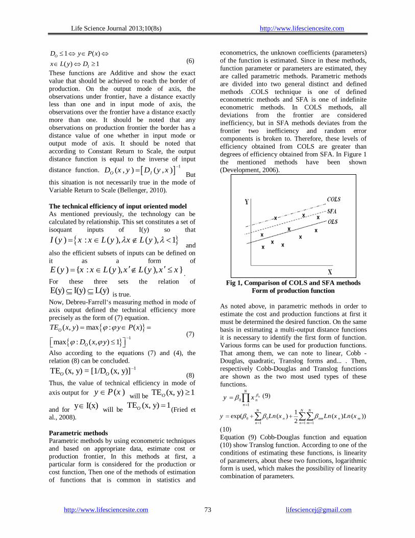
econometric methods. In COLS methods, all
deviations from the frontier are considered
inefficiency, but in SFA methods deviates from the
frontier two inefficiency and random error
components is broken to. Therefore, these levels of
efficiency obtained from COLS are greater than
degrees of efficiency obtained from SFA. In Figure 1
the mentioned methods have been shown
(Development, 2006).
Fig 1, Comparison of COLS and SFA methods
Form of production function
As noted above, in parametric methods in order to
estimate the cost and production functions at first it
must be determined the desired function. On the same
basis in estimating a multi-output distance functions
it is necessary to identify the first form of function.
Various forms can be used for production functions.
That among them, we can note to linear, Cobb - Douglas, quadratic, Translog forms and... . Then,
respectively Cobb-Douglas and Translog functions
are shown as the two most used types of these
functions.
(9)
0
1
n
N
n
n
xy
0 0
1 1 1
1exp( ( ) ( ) ( ))
2
N N N
n nm n m
n n m
y Ln x Ln x Ln x
(10)
Equation (9) Cobb-Douglas function and equation
(10) show Translog function. According to one of the
conditions of estimating these functions, is linearity
of parameters, about these two functions, logarithmic form is used, which makes the possibility of linearity
combination of parameters.

Life Science Journal 2013;10(8s) http://www.lifesciencesite.com
http://www.lifesciencesite.com [email protected] 74
(11)
0
1
( ) ( ) ( )N
n n
i
Ln y Ln Ln x
(12)
0 0
1
1 1
( ) ( )
1( ) ( )
2
N
n
n
N N
nm n m
n m
Ln y Ln x
Ln x Ln x
Equations (11) and (12) the logarithmic respectively
show the form of Cobb – Douglas and Translog
function. It is also necessary that these functions
observe two homogeneous conditions of r degree and
the symmetry in order to better estimation. For this
purpose, these conditions can be established by applying simple restrictions about the parameters. For
example, about Translog function, we can show that
this function is homogeneous from r degree, if the
constraints of equation (13) apply upon it. This
function is also symmetric if the constraints of (14)
are applied on it (Coelli, 2005).
1 1 1
0N N N
n nm nm
n n m
r and
(13)
nm nm (14)
According to the recent done researches and studies,
mainly the Translog form as a flexible form which
include input and output vectors and also the
interaction between these factors, has been used for estimation of input and output distance functions,
(Coelli and Perelman, 1999; Lovell et al., 1994;
Alvarez, 2004; Herreo, 2005). We explain this form
to estimate the distance functions.
Translog form of input distance function in multi-
output mode
Translog distance function in mode of M output and
K input is shown as form of equation (15).
0
1 1 1 1
1 1 1 1
1ln ln ln ln ln
2
1ln ln ln ln
2
1,2,3,...
M M M K
i m mi mn mi ni k ki
m m n k
K K K M
kl ki li km ki mi
k l k m
D y y y x
x x x y
i N
(15)
In equation (15) (ln D
) indicates the input distance
function of axis and I indicated the ith
firm in sample.
Also, as mentioned above, the axis input
distance function should have symmetry and Linear
Homogeneity properties. Therefore, the constraints
(16) should be imposed upon it to be homogeneous
According to the inputs from degree +1.
1
1
1
1
0, 1,2,3,...,
0, 1, 2,3,...,
K
k
k
K
kl
l
K
km
k
k K
m M
(16)
And for symmetry should be applied conditions (17) on an input-oriented distance function.
, , 1,2,...,
, , 1,2,...,
mn nm
kl lk
m n M
k l K
(17)
Using the homogeneous property was suggested in
order to make the above function estimable by Cooeli
and Perlman (1999). Homogeneity from degree +1
about inputs leads to establish the third characteristic
of following equation (18):
(0, ) ( ,0) 0I ID x and D y
A semi-continuous function is bounded from above
( , )ID y x
( , ) ( , ) 0I ID y x D y x for (18)
( , ) ( , ) 1I ID y x D y x for
( , ) ( , ) 1I ID y x D y x for
( , )ID y x is a convex function with respect to the
inputs.
Based on this property and with selecting an optional
input such as Kix
, if 1/ Kix
, all entries can be
normalized, and the condition of homogeneity from
degree +1 according to x and the input distance
function can be applied (Alvarez, 2004).
(19)
( , ) ( , )I Ki I KiD y x x D y x x
With applying condition (19) on equation (15), it can
be written in the form of equation (20). 1
0
1 1 1 1
1 1 1
1 1 1 1
1ln ( ) ln ln ln ln
2
1ln ln ln ln
2
1,2,3,...,
M M M K
Ii Ki m mi mn mi ni k ki
m m n k
K K K M
kl ki li km ki mi
k l k m
D x y y y x
x x x y
i N
(20)
In above equation k k Kx x x . Also this
equation can be shown as a simple form of (21).
ln( ) ( , , , , ) 1,...,Ii Ki i Ki iD x TL x x y i N
(21)

Life Science Journal 2013;10(8s) http://www.lifesciencesite.com
http://www.lifesciencesite.com [email protected] 75
The equation (22) can be concluded from equation
(21).
ln( ) ln( ) ( , , , , ) 1,...,Ii Ki i Ki iD x TL x x y i N
(22)
And finally the estimable input distance function of axis in multi-input and multi-output mode can be
summarized in equation (23). (Coelli and Perelman,
1999)
ln( ) ( , , , , ) ln( ) 1,...,Ki i Ki i lix TL x x y D i N
(23)
Translog form of output distance function of axis
in multi-mode output
Translog output distance function of axis including M
output and K input can also be shown as the form of
equation (24) that indicates the output distance
function of axis for the i th unit .
0
1 1 1 1
1 1 1 1
1ln ln ln ln ln
2
1ln ln ln ln
2
1,2,3,...,
M M M K
oi m mi mn mi ni k ki
m m n k
K K K M
kl ki li km ki mi
k l k m
D y y y x
x x y
i N
(24)
Output-oriented distance function according to
outputs is homogeneous from degree +1. Therefore,
constraints of (25) can be imposed upon it.
1
1
1
1
0, 1,2,3,...,
0, 1, 2,3,...,
M
m
m
M
mn
n
M
km
m
m M
k k
(25)
And for symmetry, the conditions of (26) should be
imposed on the output distance function. (Coelli and
Perelman, 1999)
, , 1,2,...,
, 1,2,...,
mn nm
kl lk
m n M
k l K
(26)
As it is mentioned about the axis input distance
function, with a choice of optional output, such as
Miy, if
1/ Miy ,all inputs can be normalized
and the condition of homogeneity from degree +1
according to Ys can be applied on the outputs distance function. (Alvarez, 2004, p77)
( , ) ( , )o M o MD x y y D x y y(27)
By applying the homogeneity condition of (27), the
output distance function can be rewritten as a form of
(28).
1 1 1
0
1 1 1 1
1
1 1 1 1
1ln ln ln ln ln
2
1ln ln ln ln
2
1,2,3,...,
M M M K
oi Mi m mi mn mi ni k ki
m m n k
K K K M
kl ki li km ki mi
k l k m
D y y y y x
x x x y
i N
(28)
That in above equation, m m My y y
. Equation (28) can be rewritten as a simple equation of (29).
ln( ) ( , , , , ) 1,...,oi Mi i i MiD y TL x y y i N
(29)
The equation (30) can be concluded from equation
(29).
ln( ) ln( ) ( , , , , ) 1,...,oi Mi i i MiD y TL x y y i N
(30)
And finally, we will have the input distance function
of estimable function in multi-input and multi-output
mode as a summarized equation (Coelli and
Perelman, 1999).
ln( ) ( , , , , ) ln( ) 1,...,Mi i i Mi oiy TL x y y D i N
(31)
3. Methodology In current research, a number of useful financial ratios are calculated by gathering information
stipulated in financial statements of companies
registered member of Stock Exchange
pharmaceutical industry. And then by performing a factor analysis on these data, the
most appropriate of them was chosen as an
indicator of efficiency measurement. Then according to approach of corrected ordinary
least squares (COLS), the research data has been
estimated by estimator of ordinary least squares (OLS) with statistical software and the
efficiency of mentioned companies were
calculated. Also, parallel with using DEA model
as one of the nonparametric methods, the efficiency of mentioned units has been solved
and modeled by the software GAMS.
Research variables
After studying and investigating literature and
history of research, some of most useful financial ratios were identified and selected as
investigated variables. About selection of
financial ratios, we should pay attention that
there are many standard ratios used for evaluating the efficiency of companies and
organizations. Selection of the best and most
Life Science Journal 2013;10(8s) http://www.lifesciencesite.com
http://www.lifesciencesite.com [email protected] 76
effective ratio to measure the efficiency of
investigated company, especially since it is important that ratios are selected somehow
involve all dimensions of financial activities of
company and provide a more accurate image of
company efficiency and performance.so in current study, the most useful ratios are selected
as research variables by careful investigation of
done studied on this field. Among these researches, we can note to Chen and Shimerda
research titled an applied analysis of useful
financial ratios, that authors have succeeded to classify and provide 41useful and important
ratios in mentioned researches by studying and
investigating 26 researches about useful
financial ratios. They indicated that the found ratios, in more current researches are known
efficient and as the criteria have been used for
measuring organizational performance have been used(Chen & Shimerda, 1981).also,
Rahman and Hossari in a similar research
,succeeded to identify 48 useful financial ratios by studying and investigating 53 scientific
researchers conducted in 1966 to 2002 (Hossari
& Rahman, 2005).
In addition to these researches, DE et al (2011) studies, Hsieh & Wang, 2001, Bhunia & Sarkar,
2011 were investigate particularly and other
conducted researches and papers about financial ratios were investigated generally and with
regard to the rate of importance and also
abundance of errands, 43 cases were selected as
the most important and useful ratios among multitudes studied ratios. In addition, it should
be mentioned that selection of mentioned ratios
has been done based on data existence in provided financial statements by stock exchange
organization and also, the use of experts’ idea
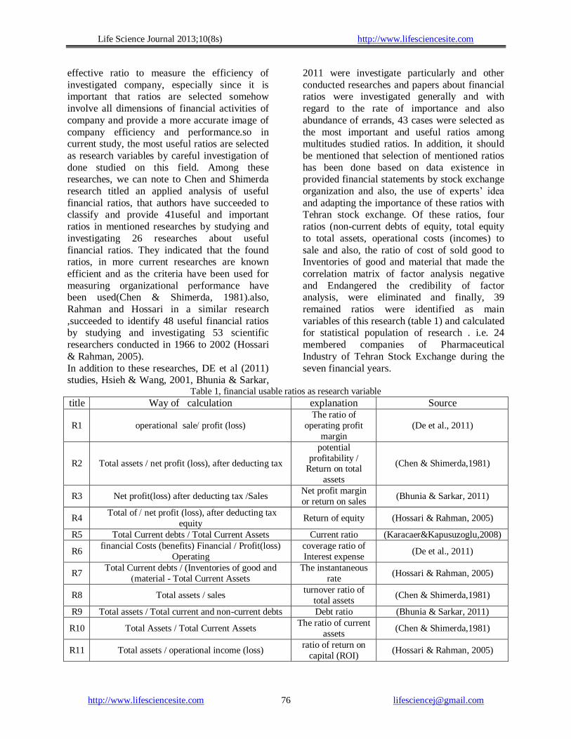
and adapting the importance of these ratios with Tehran stock exchange. Of these ratios, four
ratios (non-current debts of equity, total equity
to total assets, operational costs (incomes) to
sale and also, the ratio of cost of sold good to Inventories of good and material that made the
correlation matrix of factor analysis negative
and Endangered the credibility of factor analysis, were eliminated and finally, 39
remained ratios were identified as main
variables of this research (table 1) and calculated for statistical population of research . i.e. 24
membered companies of Pharmaceutical
Industry of Tehran Stock Exchange during the
seven financial years.
Table 1, financial usable ratios as research variable
Source explanation Way of calculation title
(De et al., 2011)
The ratio of
operating profit
margin
profit (loss) / sale operational R1
(Chen & Shimerda,1981)
potential
profitability / Return on total
assets
Total assets / net profit (loss), after deducting tax R2
(Bhunia & Sarkar, 2011) Net profit margin
or return on sales Net profit(loss) after deducting tax /Sales R3
(Hossari & Rahman, 2005) Return of equity net profit (loss), after deducting tax / Total of
equity R4
(Karacaer&Kapusuzoglu,2008) Current ratio Total Current debts / Total Current Assets R5
(De et al., 2011) coverage ratio of Interest expense
financial Costs (benefits) Financial / Profit(loss)
Operating R6
(Hossari & Rahman, 2005) The instantaneous
rate
Total Current debts / (Inventories of good and
material - Total Current Assets) R7
(Chen & Shimerda,1981) turnover ratio of
total assets Total assets / sales R8
(Bhunia & Sarkar, 2011) Debt ratio Total assets / Total current and non-current debts R9
(Chen & Shimerda,1981) The ratio of current
assets Total Assets / Total Current Assets R10
(Hossari & Rahman, 2005) ratio of return on
capital (ROI) Total assets / operational income (loss) R11

Life Science Journal 2013;10(8s) http://www.lifesciencesite.com
http://www.lifesciencesite.com [email protected] 77
(Bhunia & Sarkar, 2011) circulation ratio of
Receivable
accounts
Commercial accounts and notes receivable / sales R12
(Hossari & Rahman, 2005) Total debt Ratio Total shareholders' equity / total current and non-
current debts R13
(De et al., 2011) cash Ratio Total Current debts / cash stock R14
(Hossari & Rahman, 2005) Total Equity / Total Current debts R15
(Karacaer&Kapusuzoglu,2008) Total shareholders' equity / fixed assets after
deducting depreciation R16
(Rudposhti et al, 2011, p478) Ratio gross profit
margin Sales / gross Profit(loss) R17
(Chen & Shimerda,1981)
the ratio of Product
to of the working capital
Total Current debts - Total Current Assets) / Inventories of good and material
R18
(De et al., 2011) circulation of good
Inventory Inventories of good and material / Sales R19
(De et al., 2011) circulation rate of
Current capital (Total Current debts - Total Current Assets) / Sales R20
(Chen & Shimerda,1981) Total assets / (Total Current debts - Total Current
Assets) R21
(Bhunia & Sarkar, 2011) Sales / cash stock R22
(Hossari & Rahman, 2005) Cash profit ratio Total Current debts / cash flow R23
(Bhunia & Sarkar, 2011) ROE (return on
investment)
Total shareholders' equity / operational income
(loss) R24
(Hossari & Rahman, 2005) Market value of
equity to total debts
Total current debts and non-current debts /
((average annual stock price * number of shares) +
(capital - Total equity))
R25
(Vakili fard Fred, 2001, p 99) Ratio of (P/E)
Earnings per share after deducting tax / average
annual stock price R26
(Bhunia & Sarkar, 2011) Total assets / operational income (loss) R27
(Hossari & Rahman, 2005) The circulation
ratio current assets Total Current Assets / Sales R28
(De et al., 2011) The circulation
ratio fixed asset After deducting depreciation of fixed assets / sales R29
(Hossari & Rahman, 2005) Total shareholders' equity / sales R30
(De et al., 2011) Cash profit of on
used capital
(Total Current debts - Total assets) / stock profit
adopted by council R31
(De et al., 2011) Total assets / stock profit adopted by council R32
(De et al., 2011) Total shareholders' equity / stock profit adopted by
council R33
(De et al., 2011) (Total Current debts - Total assets) / operational
income (loss) R34
(Nikoomaram and et al, 2011, p
105) Total Current Assets / cash stock R35
(Hossari & Rahman, 2005) Total assets / cash stock R36
(Akbari, 2010, p 56) times of settling
creditors
accounts average and Commercial payable
documents at the beginning and end of the period /
(cost of goods sold - inventory of good at begining
of period + inventory of good at the end of period)
R37
(Hossari & Rahman, 2005) circulation of good
Inventory (other
method)
Average Inventories at the beginning and end of
the period / Sale R38
(Akbari, 2010, p 77) recovering demand
period
Sales / Average of accounts and receivable notes
at the beginning and end of the period * 360 R39

Life Science Journal 2013;10(8s) http://www.lifesciencesite.com
http://www.lifesciencesite.com [email protected] 78
Statistical population and sample
According to information published on the Tehran
Stock Exchange about accepted companies, currently
27 companies have been members of Pharmaceutical
Industry. Of these, three companies: Alborz Investment CO, Daroo pakhsh and Sobhan
Pharmaceutical group, are engaging in production
and distribution of Pharmaceutical, which due to
observing the congruence origin, these companies
been excluded from the research community and 24
other firms organize the statistical population of
research. The names of these companies are visible in table 2.
Table 2, the statistical society studied by research study
Row DMU Symbol Company
1 DMU1 D-Albor Alborz daroo
2 DMU2 D-Iran Iran daroo
3 DMU3 D-Pars Pars daroo
4 DMU4 D-Tamad raw materials production of
Daroupakhsh
5 DMU5 Sh-Tehran Tehran Chemistry
6 DMU6 D-Abur Abu-Reyhan pharmacy
7 DMU7 D-Osveh Osveh pharmacy
8 DMU8 D_ler Exir pharmacy
9 DMU9 D_Amin Amin pharmacy
10 DMU10 D-Tehran Tehran pharmacy
11 DMU11 D-Jaber Jaber -ebne-hayyan pharmacy
12 DMU12 D_rooz Ruz-daroo pharmacy
13 DMU13 D-Sina Sina Pharmacy
14 DMU14 D-Fara Farabi Pharmacy
15 DMU15 D-Kosar Kosar Pharmacy
16 DMU16 D-Zahravi Zahravi pharmacy
17 DMU17 D-Razak Razak medicinal
18 DMU18 D-
Loghman Loghman medicinal
19 DMU19 D-Dam Damlran
20 DMU20 D-Shimi Medicinal Chemistry of Daroupakhsh
21 DMU21 D-Fara Injection products of Iran
22 DMU22 Daroo Daroupakhsh Pharmacutical
23 DMU23 D-Kimi Kimia drug
24 DMU24 D-Abid Dr. Abidi ‘s lab of pharmacy
4. Research findings
Factor analysis on 39 identified financial ratios as the
original variables of study was done by software
version 17, SPSS, and principal component analysis
method (PCA). According to that the value of
adequacy test or sufficiency of Kayzer-Mayer-Olkin
(KMO) sampling, is equal 0.710 and also the value of
sig of Kervit Bartelt test is less than 5%, the sample size was shows appropriate for factor analysis. Also,
in order to determine the number and identification of
extracted components (factors), according to the
Kaiser criterion, we identify components that have
one or more of Eigen values. These components will
include nine first components, which explain 86.9%
of the variance of total variables. It should be noted
that the first three components of this set, have the
largest contribution in explanation of variation
(54.4%). After determining the number of components, factor
loadings (factor scores) of each variable on the
Life Science Journal 2013;10(8s) http://www.lifesciencesite.com
http://www.lifesciencesite.com [email protected] 79
remaining elements can be observed in component
matrix. Factor loadings of components Of these
tables have generally small amounts which makes
interpretation difficult, for example, in the eighth
component, none of the variables does not have
factor loadings greater than 0.5. Thus, since the interpretation of factor loadings without rotation is
not an easy task, you must turn the factors to increase
the ability of interpretation. As noted above after
number of factors was identified, the next step is to
try interpreting it. to help this process, the factors are
rotated. This action does not only change the
fundamental solutions, but also ,represents
interpretation pattern in a way that is easier .with
regarding that the purpose of applying factor analysis
in this research is reduction of variables somehow
these factors obtained from it , are not dependent
together , the use of orthogonal rotation is more suitable. Therefore, in this study, varimax rotation is
used. The results obtained from this rotation that are
visible in table (3), help to easier identification of
variables that have the most factor loading on nine
mentioned components. According to this table, the
most factors loading on the first component belongs
to R15 and on second to ninth components,
respectively belongs to R19, R10, R39, R36, R4,
R18, R5 and R26. With regarding that these ratios
have the most correlation value with related factors,
they can be selected as a reagent of each factor. So, it is expected that by using these nine variables, the
manner of other available ratios on the same level,
can be explained logically. This approach has been
used in previous research such as: Tuna and others
(1997) ,Yarbod (2007) and (De et al., 2011; Tan et
al., 1997). Accordingly, 39 selected ratios have been
reduced to nine ratios obtained from Varimax
rotation and furthermore, they are applied in order to
evaluate the efficiency measurement of 24 studied
companies.
Measurement efficiency
After identifying the main research variables through factor analysis, in this part, efficiency of the
pharmaceutical companies on the stock exchange will
be measured by data envelopment analysis.
According to sensitivity of DEA model to variables’
selection, the most important issue in this part is the
Grouping of identified ratios into two groups of input
and output variables in the previous section.
Unfortunately, the majority of accomplished
researches in this field, no consistent approach and
methodology have been introduced to identify the
inputs and outputs and researchers mainly have applied this classification by their own opinions, far
as some of ratios have been classified in a research
titled as an output variable and in other research titled
as an input variable. Malhtra approach has been used
in this study.according to Malhatra (2008) and
Vertingten (1998), ratios that their increasing means
the efficiency of company as an output and ratios that
their reduction means better performance as input of
DEA and COLS models were used. (Malhotra D.K.
& Malhotra R., 2008; Worthington, 1998). Also, this approach, consistent with the definitions of
Koompanz ,Debro and Farrel about technical
efficiency .so, the literature of topic has been
investigated and according the desirability of being
increased or decreased of nine ratios obtained factor
analysis ,these ratios are divided to two groups of
input and output. Then this classification is titles in
detail and with reference to the nature of mentioned
ratios.
Input ratios
1) Ratio of current assets to total assets (R10),
Any increase in this ratio is lead to reduce
the profitability of the enterprise, because it
is assumed that the ratio of current assets to
fixed assets will lead to less profitability
(Khan, 2004).
2) The ratio of total current debts to total equity
(R15), this ratio indicated the relation of
debt and Eigen values (total equity).when
this ratio is high, the diagnosis is undesirable
and its continuous increase will require
revising in manner of combining investors
(Akbari, 2010)
3) Ratios of good to working capital (R18), this
ratio indicates that some percentage of
working capital is changed to goods
inventory. High percentage is considered as
an indication of existence of problem in
circulating current operation (Akbari, 2010).
4) The period of demands recovery (R39), this
ratio is calculated based on day and
indicates that on average it will take a few
days to recovery the demands from credit
sales. If this ratio is smaller, it is better,
because by faster recovering the demands,
speed of short-term obligations is increased
(conditioned beliefs, 2010).
Output ratios
1) The ratio of cash to total assets (R36), as one
of liquidity ratios, shows the company's
ability to provide needed cash to pay its
debts to creditors. Hence, if this ratio
allocates greater amount, the probability of

Life Science Journal 2013;10(8s) http://www.lifesciencesite.com
http://www.lifesciencesite.com [email protected] 80
financial distress is reduced. It should also
be paid attention that current assets (like
cash), have less ability to profitability.
Therefore, companies should try balancing
among these assets, create an optimum
combination to earn maximum profits and
reducing risk, (wahlen, Baginski, Bradshaw,
2008). Is necessary to explain that existence
of ratio of current assets to total assets (R10)
as one of the inputs of model will help to
establish this balance. Because In case of the
excessive increase of cash balance, And
consequently increasing rate of R36, R10
rate has also increased that with regard to its
nature as an input variable, increasing R10
provides efficiency reductions.
2) R26 ratio, which shows the relationship
between annual stock price and earnings per
share after deducting tax. This ratio is one of
most important scales of stock evaluation
that can be used by investors in the market.
This low ratio indicates that the share of this
article, is not very appropriate and the high
ratio can indicate its favorable position in
the market share. (vakili fard, 2001). It is
Necessary to explain that this ratio like other
financial ratios cannot be the ultimate
criterion alone for evaluation and should be
investigated in the presence of other factors.
3) Current ratio of R5 that is obtained from
division of current assets to current company
debts indicated the ability of company to
pay its debts to creditors. Increase in this
ratio indicates that creditors will have more
confidence about receiving their own
demand to get (Nikoo maram, 2010).
4) Inventory rotation ratio of good R19, which
can be used to calculate two commonly
methods. Both methods were used in this
study that results of the first method i.e.
division of Sales to good Inventories is
reflected in ratio R19, And the results of the
second method; division of sold goods on
good inventory, is visible by R38 ratio.it is
nesseccary to mentioned that R19 and R38
factor loading to sixth factor, are very close
together and In simple terms, the ratio of
these two can be used interchangeably. It
should also be noted that, typically, a high
inventory rotation ratio is an indication of a
company's management efficiency. If all
other factors are constant, the much rotation
flow is more desirable than low-rotation
ratio (Novo, 2001).
5) Net profit to equity ratio (R4), that if this
ratio is higher, the profitable unit has a
better performance and therefore has greater
efficiency, and consequently, productivity of
business unit is higher than financial
perspective (Nikoomaram, 2010).
DEA results
After determining input and output variables in this
section, by using data envelopment analysis models
that were discussed above, we calculate efficiency of
24 companies of statistical population of research.
For this purpose, BCC and CCR methods by GAMS
software have been modeled and solved in two input and output modes during financial years of 2003 to
2009, and their results are visible in following tables.
Input and output oriented CCR models
According to the same obtained results of input and
output oriented CCR model, it is showed only input
oriented model (see table 3).
Table 3, CCR DEA model results (2003-2006)
2003 2004 2005 2006
DMU 1 65.55% 70.15% 70.06% 65.02%
DMU 2 100.00% 100.00% 100.00% 100.00%
DMU 3 93.04% 100.00% 100.00% 100.00%
DMU 4 100.00% 100.00% 100.00% 100.00%
DMU 5 68.36% 62.43% 49.67% 64.90%
DMU 6 100.00% 94.97% 100.00% 100.00%
DMU 7 77.43% 73.81% 100.00% 100.00%

Life Science Journal 2013;10(8s) http://www.lifesciencesite.com
http://www.lifesciencesite.com [email protected] 81
DMU 8 100.00% 84.23% 69.68% 66.23%
DMU 9 61.14% 58.92% 93.75% 100.00%
DMU 10 70.19% 84.23% 96.31% 89.37%
DMU 11 80.82% 100.00% 100.00% 100.00%
DMU 12 100.00% 100.00% 93.38% 100.00%
DMU 13 100.00% 100.00% 100.00% 100.00%
DMU 14 86.22% 73.47% 70.95% 80.27%
DMU 15 75.51% 66.90% 67.33% 78.55%
DMU 16 73.97% 81.78% 100.00% 100.00%
DMU 17 94.28% 71.74% 72.74% 68.62%
DMU 18 100.00% 89.05% 63.12% 57.43%
DMU 19 61.29% 63.20% 69.41% 53.89%
DMU 20 100.00% 100.00% 70.44% 61.09%
DMU 21 100.00% 100.00% 100.00% 99.86%
DMU 22 63.52% 52.69% 66.34% 67.09%
DMU 23 64.67% 63.56% 82.73% 99.33%
DMU 24 100.00% 100.00% 100.00% 100.00%
Continue Table 3, CCR DEA model results (2007-2009)
2007 2008 2009
DMU 1 100.00% 100.00% 100.00%
DMU 2 80.96% 100.00% 81.73%
DMU 3 100.00% 100.00% 100.00%
DMU 4 91.67% 88.10% 89.00%
DMU 5 86.73% 59.72% 99.49%
DMU 6 100.00% 77.63% 74.79%
DMU 7 100.00% 100.00% 100.00%
DMU 8 77.69% 86.14% 82.66%
DMU 9 59.76% 67.66% 91.49%
DMU 10 78.03% 95.07% 69.00%
DMU 11 100.00% 100.00% 100.00%
DMU 12 100.00% 100.00% 100.00%
DMU 13 100.00% 100.00% 100.00%
DMU 14 71.47% 77.99% 80.55%
DMU 15 78.31% 91.01% 90.23%
DMU 16 100.00% 100.00% 100.00%
DMU 17 86.88% 100.00% 95.97%
DMU 18 94.79% 76.35% 100.00%
DMU 19 63.84% 67.59% 67.82%
DMU 20 66.17% 77.58% 100.00%
DMU 21 100.00% 100.00% 100.00%

Life Science Journal 2013;10(8s) http://www.lifesciencesite.com
http://www.lifesciencesite.com [email protected] 82
DMU 22 73.80% 77.64% 95.11%
DMU 23 90.87% 80.65% 74.77%
DMU 24 86.37% 100.00% 100.00%
As shown in Table (3) in 2003, among 24
investigated companies, 10 companies have
efficiency equal one. Similarly, in 2004 to 2008,
respectively, 9, 10, 11, 9, 11 and 11 units have been
identified as efficient units. The lowest level of
efficiency in 2003 belongs to DMU9 and is equal
61.14%.
Similarly, for 2004 to 2009 respectively, the DMUs of 22 with 52.69%, 5 with 49.67%, 19 with 53.89%,
and9 with 59.76%, 19 with 67.82% and 5 with
59.72%, have the lowest efficiency range among the
companies under investigation. It is noteworthy that
DMUs of both 5 and 9 for 2 years were the most
inefficient companies and the lowest efficiency range
obtained from CCR model in 7 years, belongs to
DMU of 5 in 2005. The only company that during
period of 7 years has 100% efficiency, is DMU of 13
and then it can pointed to DMU of 21 that only in
2006 has 99.86 % efficiency and in other financial
years has 100% efficiency.
Input oriented BCC model
In this section like the previous section, by using four inputs and five outputs, efficiency of membered
companies of Pharmaceutical Industry is gauged. For
this purpose, BCC model of the input of axis is used.
The obtained results of solving this model can be
observed by GAMS software in Table (4).
Table 4, results of BCC model of input and output oriented (2003-2006)
2003 2004 2005 2006
Out In Out In Out In Out In
DMU 1 76 70 96 80 96 89 87 68
DMU 2 100 100 100 100 100 100 100 100
DMU 3 95 98 100 100 100 100 100 100
DMU 4 100 100 100 100 100 100 100 100
DMU 5 100 100 82 96 53 83 100 100
DMU 6 100 100 100 100 100 100 100 100
DMU 7 81 90 75 85 100 100 100 100
DMU 8 100 100 87 86 97 73 92 69
DMU 9 73 80 92 60 100 100 100 100
DMU 10 71 78 85 88 100 100 96 90
DMU 11 86 85 100 100 100 100 100 100
DMU 12 100 100 100 100 95 94 100 100
DMU 13 100 100 100 100 100 100 100 100
DMU 14 88 95 74 83 75 79 82 88
DMU 15 77 84 67 81 75 76 83 85
DMU 16 77 79 84 92 100 100 100 100
DMU 17 100 100 84 76 91 75 84 74
DMU 18 100 100 100 100 81 64 61 74
DMU 19 71 74 64 74 75 74 72 64
Life Science Journal 2013;10(8s) http://www.lifesciencesite.com
http://www.lifesciencesite.com [email protected] 83
DMU 20 100 100 100 100 81 78 72 70
DMU 21 100 100 100 100 100 100 100 100
DMU 22 65 72 64 66 77 71 78 74
DMU 23 73 78 65 78 87 85 100 100
DMU 24 100 100 100 100 100 100 100 100
Continue Table 4, results of BCC model of input and output oriented (2007-2009)
2007 2008 2009
Out In Out In Out In
DMU 1 100 100 100 100 100 100
DMU 2 92 81 100 100 86 85
DMU 3 100 100 100 100 100 100
DMU 4 93 92 90 88 90 92
DMU 5 100 100 67 93 100 100
DMU 6 100 100 78 86 77 81
DMU 7 100 100 100 100 100 100
DMU 8 94 80 99 87 92 83
DMU 9 70 71 74 76 93 95
DMU 10 91 97 100 100 70 90
DMU 11 100 100 100 100 100 100
DMU 12 100 100 100 100 100 100
DMU 13 100 100 100 100 100 100
DMU 14 81 77 83 83 85 86
DMU 15 81 82 91 97 95 91
DMU 16 100 100 100 100 100 100
DMU 17 95 87 100 100 97 96
DMU 18 97 95 81 93 100 100
DMU 19 84 65 87 72 79 73
DMU 20 73 72 90 79 100 100
DMU 21 100 100 100 100 100 100
DMU 22 84 74 83 79 95 95
DMU 23 97 92 86 88 82 81
DMU 24 92 92 100 100 100 100
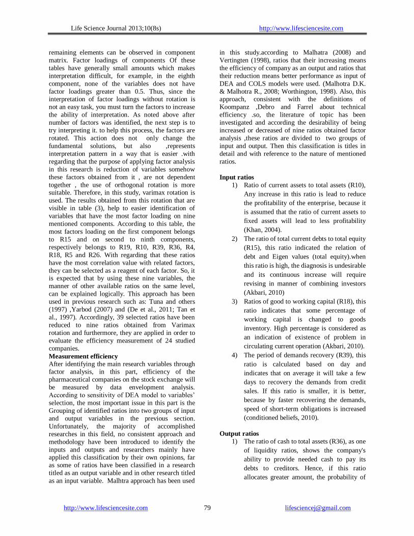
As shown in Table (4) in 2003, among the surveyed companies, 12 companies have an efficiency equal
one. Similarly, in 2004 to 2009, respectively, 11, 12, 14, 10, 12 and 12 units have been identified as
Life Science Journal 2013;10(8s) http://www.lifesciencesite.com
http://www.lifesciencesite.com [email protected] 84
efficient units. The lowest level of efficiency in 2003
belongs to DMU of 1 and is equal 69.73%. Similarly,
for 2004 to 2009, respectively, the DMUs of 9 with
60.03%, 18 with 64.32 % , 19 with 64.22 % , 19 with
65.15 %,19 with 71.63% and 19 with 72.89% , have
the lowest efficiency among the investigated companies . It is noteworthy that DMUs of 19 has
been the most inefficient company for four
consecutive years and the lowest efficiency obtained
from BCC model of input of axis during seven years
belongs to DMU9 in 2001.DMUs of 13 and 21 seven
years period, had 100% efficiency based on this
model and after them, DMUs of 3, 12 and 24 After
the DMU 3, 12 and 24 have shown the best
performance in this period. DMU of 3 only had
98.05% efficiency in 2003 and has 100% efficiency
in other financial year. DMU of 12 except in 2005
that had 93.51% efficiency also has been completely efficient in other years. DMU of 24 had 91.67%
efficiency in 2007 and in the rest years of the
reviewing period was 100% percent efficient. By
comparing BCC method of axis input and CCR
method, it can be seen that more units have been
identified efficient by BCC method and also in this
method, there is a less distance between inefficient
and efficient companies in comparison to CCR model
that this is due to returns to variable scale of model
BCC. As shown in Table (4), the number of units in
each financial year has been identified effective, exactly like the mode of axis input of BCC model.
Also the lowest level of efficiency in 2003 belongs to
DMU of 22 and is equal 65.24%. Also for 2004 to
2009, respectively, the DMU 19 with 63.56%, 5 with
53.14%, 18 with 60.80%, 9 with 69.94%, 5 with
66.61% and 10 with 69.94% had the lowest
efficiency among the investigated companies. It is
noteworthy that DMU5 has been the most inefficient
company in two years and for a seven years period,
the lowest level of efficiency obtained from BCC
model of output of axis belongs to this unit in 2005.
In a state of output of axis like the input mode of
axis, DMUs of 13 and 21 during the period of 7 years
had 100% efficiency and after them, DMUs of 3, 12
and 24 have shown their own best performance.
DMU of 3 only had 95.50% efficiency in 2003 and
on other fiscal years had100% efficiency. DMU of 12, except in 2005 that had 94.71% efficiency, also
was quite efficient in other years. DMU of 24 had
92.24% efficiency in 2007 and in the rest years of the
period of reviewing, was 100 % efficient. By
comprising BCC method of axis input with axis
output of this model and also results of CCR model ,
it can be seen that there is a less distance between
efficient and in efficient companies. It indicates that
if desired companies decrease their input ratios, they
can improve the efficiency more than the time of
their increasing output ratios.
Results of model-based on techniques COLS
As discussed in detail in Chapter Two, estimation of
distance function by COLS techniques, in two modes
of input axis and output axis is possible. It is
expected that efficiency results obtained from these
two modes, assuming returns to variable scale, differ
from each other. On this basis, in this part in order to
measure the efficiency of surveyed units, estimating
the distance function has been done in both modes.
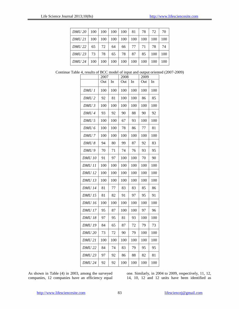
Solving input oriented COLS In the present study, according to previous studies, Translog distance function order to estimate the
efficiency of surveyed units has been selected. Also
input and output vectors, like last part, are extracted
and used from obtained results of factor analysis. So
by considering vector of input variables, including
four financial ratios R10, R15, R18 and R39 and
vector of output variables consisting of five financial
ratios R4, R5, R19, R26 and R36, Translog estimable
distance function in mode of axis input, can be shown
as equation (32)
.5 5 5 4
1 0 1
1 1 1 2
4 4 4 5
1 1 1
2 2 2 1
1ln ( ) ln ln ln ln( )
2
1ln( ) ln( ) ln( ) ln
2
1,2,3,..., 24
Ii i m mi mn mi ni k ki i
m m n k
kl ki i li i km ki i mi
k l k m
D x y y y x x
x x x x x x y
i
(32) By estimating equation (32) by constrained OLS and
consideration of assumptions (1) and (2) , the initial
parameters of function of axis input can be estimated.
For this purpose, SAS (statistical analysis software)
was used that is one of the powerful statistical
software in field of estimating regression functions.
With the help of this software, data from 2003 to
2009 of all companies is used as a panel data set.
Thus, 168 calculated data for each research variable
has entered in equation (32) and we estimate the
parameters of this model. The results obtained from
estimating mentioned function, have been shown
briefly at table (5).
Life Science Journal 2013;10(8s) http://www.lifesciencesite.com
http://www.lifesciencesite.com [email protected] 85
4
2
5
1
2
1
0, 1,2,3,...,5
0, 1, 2,3,...,5
k
k
kl
l
K
km
k
k
m
(1)
, , 1,2,...,5
, , 2,..., 4
mn nm
kl lk
m n
k l
(2)
, , 1,2,...,5
, , 2,..., 4
mn nm
kl lk
m n
k l
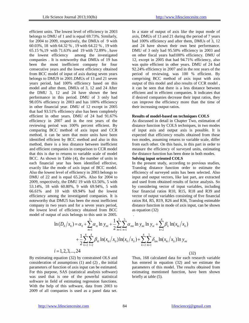
As at the end of table (5) can be seen, the results of
statistical tests ordinary least squares estimator of
constrained statistical tests, respectively for test the
goodness of fit index, or the equivalent of 92.89%,
which shows that in about 93% of variability by Translog the other explanatory variables, is
explained. As at the end of table (5) can be seen, the
results of statistical tests of estimator of constrained
ordinary least squares, respectively for test of
coefficient of goodness or determining of fit is equal
92.89%, which shows that in about 93% of changes
of dependent variable is explained by other
explanatory variables of Translog function. To
express better, we can show that based on Entry form
of distance function, about 93% observations in
estimation are true. Also according to the
descriptions presented in the second season, due to
the increasing number of model parameters, the
adjusted coefficient 2 R should be calculated for this
estimation. The result of calculation of this
coefficient shows that the goodness of done
estimation fit is more than 90% by constrained OLS.
Results of test of meaningfulness of overall multiple
regression (F test), shows that at meaningfulness
level of 99%, the assumption of
0 1 2: ... 0 kH , which is based on no
relation between independent and dependent
variables, has been refused and the opposite
assumption, 1H , has been accepted. Also a large
number of parameters estimated in this model, based
on the t-test at 95% level are recognized meaningful.
Finally, it can be concluded that based on these tests,
the estimated line is fitting well by OLS.
Table 5, estimated parameters obtained from OLS method for in and output oriented of distance function
Parameter Cols coefficient rate Parameter Parameter
Output Oriented Input Oriented Output Oriented Input Oriented
0 -2.95 -2.97
44 0.004 0.07
1 - 0.42
45 -0.03 -0.005
2 0.24
0.35 51 - 0.04
3 0.45 0.54 52 0.04 0.01
4 0.48 -0.30 53 0.01 0.01
5 -0.17 -0.12 54 -0.03 -0.005
11 - 1.73 55 0.01 -0.02
12
-
-0.06
2 0.04 -0.11
13 -
0.05
3 0.42 0.24
14 -
0.15
4 0.50 0.86
15 -
0.04
11 1.85 -
21 -
-0.06
12 -0.54 -
22 -0.05 -0.01 13 0.13 -
23 0.06 -0.02 14 0.12 -
24 -0.04 0.04 21
-0.54 -
25 0.04 0.01 22 0.08 0.48
31 -
0.05
23 -0.01 -0.04

Life Science Journal 2013;10(8s) http://www.lifesciencesite.com
http://www.lifesciencesite.com [email protected] 86
32 0.06 -0.02 24 -0.001 -0.13
33 -0.05 -0.02 31 0.13 -
34 0.008 0.002 32 -0.01 -0.04
35 0.01
0.01 33 -0.02 -0.008
41 - 0.15 34 -0.03 -0.01
42 -0.04 0.04 41 0.12 -
43 0.008 0.002 42 -0.001 -0.13
2 R %
98.15 92.89 F Value
2 R %
97.55 90.58 Pr > F
Continue Table 5, estimated parameters obtained from OLS method for in and output oriented of distance function
Parameter Cols coefficient rate
Output Oriented Input Oriented
43 -0.01 -0.03
44 -0.09 -0.04
12 -
0.18
13 -
0.11
14 -
0.07
15 -
-0.01
21 0.64 -
22 -0.06 -0.05
23 0.02 0.001
24 0.03 0.005
25 0.01 0.01
31 -0.12 -
32 -0.05 -0.10
33 -0.01 -0.04
34 -0.01 -0.06
35 -0.004 -0.01
41 -0.38 -
42 -0.008 0.01
43 -0.08 -0.05
44 0.04 -0.09
45 -0.004 0.03
40.18 163.30
<.0001 <.0001
Life Science Journal 2013;10(8s) http://www.lifesciencesite.com
http://www.lifesciencesite.com [email protected] 87
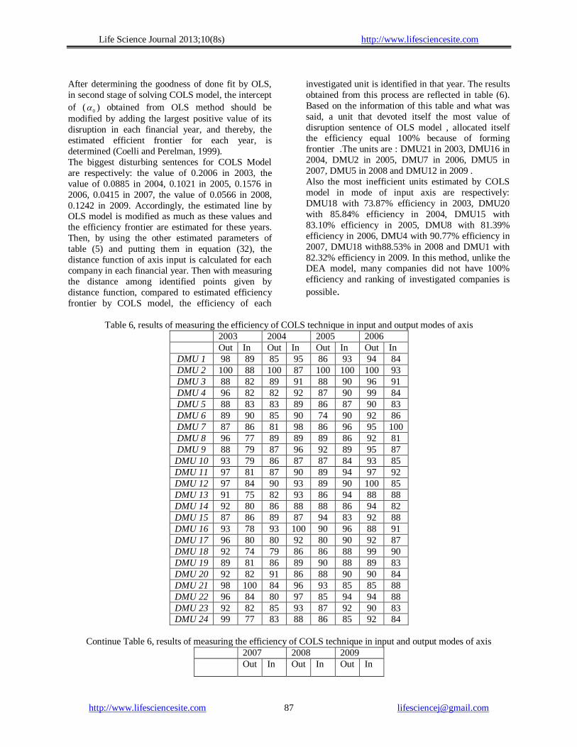
After determining the goodness of done fit by OLS,
in second stage of solving COLS model, the intercept
of ( 0 ) obtained from OLS method should be
modified by adding the largest positive value of its
disruption in each financial year, and thereby, the
estimated efficient frontier for each year, is
determined (Coelli and Perelman, 1999).
The biggest disturbing sentences for COLS Model
are respectively: the value of 0.2006 in 2003, the
value of 0.0885 in 2004, 0.1021 in 2005, 0.1576 in
2006, 0.0415 in 2007, the value of 0.0566 in 2008,
0.1242 in 2009. Accordingly, the estimated line by OLS model is modified as much as these values and
the efficiency frontier are estimated for these years.
Then, by using the other estimated parameters of
table (5) and putting them in equation (32), the
distance function of axis input is calculated for each
company in each financial year. Then with measuring
the distance among identified points given by
distance function, compared to estimated efficiency
frontier by COLS model, the efficiency of each
investigated unit is identified in that year. The results
obtained from this process are reflected in table (6).
Based on the information of this table and what was
said, a unit that devoted itself the most value of
disruption sentence of OLS model , allocated itself the efficiency equal 100% because of forming
frontier .The units are : DMU21 in 2003, DMU16 in
2004, DMU2 in 2005, DMU7 in 2006, DMU5 in
2007, DMU5 in 2008 and DMU12 in 2009 .
Also the most inefficient units estimated by COLS
model in mode of input axis are respectively:
DMU18 with 73.87% efficiency in 2003, DMU20
with 85.84% efficiency in 2004, DMU15 with
83.10% efficiency in 2005, DMU8 with 81.39%
efficiency in 2006, DMU4 with 90.77% efficiency in
2007, DMU18 with88.53% in 2008 and DMU1 with
82.32% efficiency in 2009. In this method, unlike the DEA model, many companies did not have 100%
efficiency and ranking of investigated companies is
possible.
Table 6, results of measuring the efficiency of COLS technique in input and output modes of axis
2003 2004 2005 2006
Out In Out In Out In Out In
DMU 1 98 89 85 95 86 93 94 84
DMU 2 100 88 100 87 100 100 100 93
DMU 3 88 82 89 91 88 90 96 91
DMU 4 96 82 82 92 87 90 99 84
DMU 5 88 83 83 89 86 87 90 83
DMU 6 89 90 85 90 74 90 92 86
DMU 7 87 86 81 98 86 96 95 100
DMU 8 96 77 89 89 89 86 92 81
DMU 9 88 79 87 96 92 89 95 87
DMU 10 93 79 86 87 87 84 93 85
DMU 11 97 81 87 90 89 94 97 92
DMU 12 97 84 90 93 89 90 100 85
DMU 13 91 75 82 93 86 94 88 88
DMU 14 92 80 86 88 88 86 94 82
DMU 15 87 86 89 87 94 83 92 88
DMU 16 93 78 93 100 90 96 88 91
DMU 17 96 80 80 92 80 90 92 87
DMU 18 92 74 79 86 86 88 99 90
DMU 19 89 81 86 89 90 88 89 83
DMU 20 92 82 91 86 88 90 90 84
DMU 21 98 100 84 96 93 85 85 88
DMU 22 96 84 80 97 85 94 94 88
DMU 23 92 82 85 93 87 92 90 83
DMU 24 99 77 83 88 86 85 92 84
Continue Table 6, results of measuring the efficiency of COLS technique in input and output modes of axis
2007 2008 2009
Out In Out In Out In

Life Science Journal 2013;10(8s) http://www.lifesciencesite.com
http://www.lifesciencesite.com [email protected] 88
DMU 1 97 95 88 94 94 82
DMU 2 92 94 88 93 93 88
DMU 3 90 95 93 96 93 87
DMU 4 95 91 91 92 93 89
DMU 5 100 100 90 100 100 89
DMU 6 87 98 87 93 95 87
DMU 7 99 97 100 96 97 85
DMU 8 95 91 95 99 94 89
DMU 9 89 95 91 96 93 91
DMU 10 93 94 95 94 94 88
DMU 11 95 95 91 91 96 89
DMU 12 92 92 86 100 92 100
DMU 13 93 95 88 98 99 89
DMU 14 91 95 90 94 93 85
DMU 15 89 96 95 93 94 86
DMU 16 93 96 97 98 93 89
DMU 17 91 95 95 94 98 88
DMU 18 95 93 88 89 91 89
DMU 19 90 94 88 91 93 86
DMU 20 97 94 93 93 97 90
DMU 21 85 94 89 94 96 86
DMU 22 96 100 95 98 96 90
DMU 23 93 93 88 94 93 88
DMU 24 91 92 91 94 94 87
Solving the output oriented model of COLS
After estimating the mode of axis input technique of
COLS, in this stage by considering vector of input
and output variables used in previous sections,
Translog distance function in mode of axis output can
be shown as an estimable form in equation (33). 5 5 5 4
1 0 1 1 1
2 2 2 1
4 4 4 5
1
1 1 1 2
1ln( ) ln( ) ln( ) ln( ) ln
2
1ln ln ln ln( )
2
1,2,3,..., 24
oi i m mi i mn mi i ni i k ki
m m n k
kl ki li km ki mi i
k l k m
D y y y y y y y x
x x x y y
i
(33)
Like the mode of input axis, according to
assumptions (3) and (4), with the help of constrained
OLS, the equation (33) can be estimated. 5
2
5
2
5
2
1
0, 2,3,...,5
0, 1, 2,3,4
m
m
mn
n
km
m
m
k
(3)
, , 2,...,5
, , 1,2,..., 4
mn nm
kl lk
m n
k l
(4)
Life Science Journal 2013;10(8s) http://www.lifesciencesite.com
http://www.lifesciencesite.com [email protected] 89
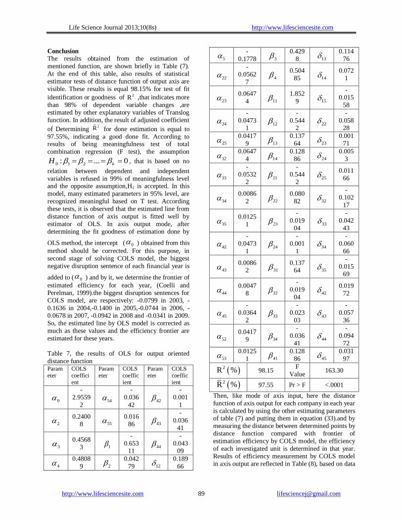
Conclusion
The results obtained from the estimation of
mentioned function, are shown briefly in Table (7).
At the end of this table, also results of statistical
estimator tests of distance function of output axis are
visible. These results is equal 98.15% for test of fit
identification or goodness of 2 R ,that indicates more
than 98% of dependent variable changes ,are
estimated by other explanatory variables of Translog
function. In addition, the result of adjusted coefficient
of Determining 2 R for done estimation is equal to
97.55%, indicating a good done fit. According to results of being meaningfulness test of total
combination regression (F test), the assumption
0 1 2: ... 0 kH , that is based on no
relation between dependent and independent
variables is refused in 99% of meaningfulness level and the opposite assumption,H1 is accepted. In this
model, many estimated parameters in 95% level, are
recognized meaningful based on T test. According
these tests, it is observed that the estimated line from
distance function of axis output is fitted well by
estimator of OLS. In axis output mode, after
determining the fit goodness of estimation done by
OLS method, the intercept ( 0 ) obtained from this
method should be corrected. For this purpose, in
second stage of solving COLS model, the biggest
negative disruption sentence of each financial year is
added to ( 0 ) and by it, we determine the frontier of
estimated efficiency for each year, (Coelli and
Perelman, 1999).the biggest disruption sentences for
COLS model, are respectively: -0.0799 in 2003, -
0.1636 in 2004,-0.1400 in 2005,-0.0744 in 2006, -
0.0678 in 2007, -0.0942 in 2008 and -0.0341 in 2009.
So, the estimated line by OLS model is corrected as
much as these values and the efficiency frontier are
estimated for these years.
Table 7, the results of OLS for output oriented
distance function Parameter
COLS coefficient
Parameter
COLS coefficient
Parameter
COLS coefficient
0 -
2.9559
2 54
-
0.036
42 42
-
0.001
1
2 0.2400
8 55 0.016
86 43 -
0.036
41
3 0.4568
3 1 -
0.65311
44 -
0.04309
4 0.4808
9 2 0.042
79 12 0.189
66
5 -
0.1778 3 0.429
8 13 0.114
76
22 -
0.0562
7 4
0.504
85 14 0.072
1
23 0.0647
4 11 1.852
9 15 -
0.015
58
24 -
0.04731
12 -
0.5442
22 -
0.05828
25 0.0417
9 13 0.137
64 23 0.001
71
32 0.0647
4 14 0.128
86 24 0.005
3
33 -
0.0532
2 21
-
0.544
2 25
0.011
66
34 0.0086
2 22 0.080
82 32 -
0.102
17
35 0.0125
1 23 -
0.019
04 33
-
0.042
43
42 -
0.0473
1 24
-
0.001
1 34
-
0.060
66
43 0.0086
2 31 0.137
64 35 -
0.015
69
44 0.0047
8 32 -
0.019
04 42
0.019
72
45 -
0.0364
2 33
-
0.023
03 43
-
0.057
36
52 0.0417
9 34 -
0.036
41 44
-
0.094
72
53 0.0125
1 41 0.128
86 45 0.031
97
2 R %
98.15 F
Value 163.30
2 R %
97.55 Pr > F <.0001
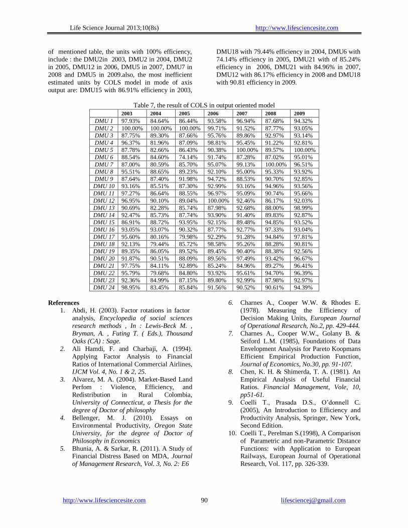
Then, like mode of axis input, here the distance
function of axis output for each company in each year
is calculated by using the other estimating parameters of table (7) and putting them in equation (33).and by
measuring the distance between determined points by
distance function compared with frontier of
estimation efficiency by COLS model, the efficiency
of each investigated unit is determined in that year.
Results of efficiency measurement by COLS model
in axis output are reflected in Table (8), based on data
Life Science Journal 2013;10(8s) http://www.lifesciencesite.com
http://www.lifesciencesite.com [email protected] 90
of mentioned table, the units with 100% efficiency,
include : the DMU2in 2003, DMU2 in 2004, DMU2
in 2005, DMU12 in 2006, DMU5 in 2007, DMU7 in
2008 and DMU5 in 2009.also, the most inefficient
estimated units by COLS model in mode of axis
output are: DMU15 with 86.91% efficiency in 2003,
DMU18 with 79.44% efficiency in 2004, DMU6 with
74.14% efficiency in 2005, DMU21 with of 85.24%
efficiency in 2006, DMU21 with 84.96% in 2007,
DMU12 with 86.17% efficiency in 2008 and DMU18
with 90.81 efficiency in 2009.
Table 7, the result of COLS in output oriented model
2003 2004 2005 2006 2007 2008 2009
DMU 1 97.93% 84.64% 86.44% 93.58% 96.94% 87.68% 94.32%
DMU 2 100.00% 100.00% 100.00% 99.71% 91.52% 87.77% 93.05%
DMU 3 87.75% 89.30% 87.66% 95.76% 89.86% 92.97% 93.14%
DMU 4 96.37% 81.96% 87.09% 98.81% 95.45% 91.22% 92.81%
DMU 5 87.78% 82.66% 86.43% 90.38% 100.00% 89.57% 100.00%
DMU 6 88.54% 84.60% 74.14% 91.74% 87.28% 87.02% 95.01%
DMU 7 87.00% 80.59% 85.70% 95.07% 99.13% 100.00% 96.51%
DMU 8 95.51% 88.65% 89.23% 92.10% 95.00% 95.33% 93.92%
DMU 9 87.64% 87.40% 91.98% 94.72% 88.53% 90.70% 92.85%
DMU 10 93.16% 85.51% 87.30% 92.99% 93.16% 94.96% 93.56%
DMU 11 97.27% 86.64% 88.55% 96.97% 95.09% 90.74% 95.66%
DMU 12 96.95% 90.10% 89.04% 100.00% 92.46% 86.17% 92.03%
DMU 13 90.69% 82.28% 85.74% 87.98% 92.68% 88.00% 98.99%
DMU 14 92.47% 85.73% 87.74% 93.90% 91.40% 89.83% 92.87%
DMU 15 86.91% 88.72% 93.95% 92.15% 89.48% 94.85% 93.52%
DMU 16 93.05% 93.07% 90.32% 87.77% 92.77% 97.33% 93.04%
DMU 17 95.60% 80.16% 79.98% 92.29% 91.28% 94.84% 97.81%
DMU 18 92.13% 79.44% 85.72% 98.58% 95.26% 88.28% 90.81%
DMU 19 89.35% 86.05% 89.52% 89.45% 90.40% 88.38% 92.56%
DMU 20 91.87% 90.51% 88.09% 89.56% 97.49% 93.42% 96.67%
DMU 21 97.75% 84.11% 92.89% 85.24% 84.96% 89.27% 96.41%
DMU 22 95.79% 79.68% 84.80% 93.92% 95.61% 94.70% 96.39%
DMU 23 92.36% 84.99% 87.15% 89.80% 92.99% 87.98% 92.97%
DMU 24 98.95% 83.45% 85.84% 91.56% 90.52% 90.61% 94.39%
References
1. Abdi, H. (2003). Factor rotations in factor
analysis, Encyclopedia of social sciences
research methods , In : Lewis-Beck M. ,
Bryman, A. , Futing T. ( Eds.), Thousand
Oaks (CA) : Sage.
2. Ali Hamdi, F. and Charbaji, A. (1994).
Applying Factor Analysis to Financial
Ratios of International Commercial Airlines, IJCM Vol. 4, No. 1 & 2, 25.
3. Alvarez, M. A. (2004). Market-Based Land
Perfom : Violence, Efficiency, and
Redistribution in Rural Colombia,
University of Connecticut, a Thesis for the
degree of Doctor of philosophy
4. Bellenger, M. J. (2010). Essays on
Environmental Productivity, Oregon State
University, for the degree of Doctor of
Philosophy in Economics 5. Bhunia, A. & Sarkar, R. (2011). A Study of
Financial Distress Based on MDA, Journal
of Management Research, Vol. 3, No. 2: E6
6. Charnes A., Cooper W.W. & Rhodes E.
(1978). Measuring the Efficiency of
Decision Making Units, European Journal
of Operational Research, No.2, pp. 429-444.
7. Charnes A., Cooper W.W., Golany B. &
Seiford L.M. (1985), Foundations of Data
Envelopment Analysis for Pareto Koopmans
Efficient Empirical Production Function,
Journal of Economics, No.30, pp. 91-107. 8. Chen, K. H. & Shimerda, T. A. (1981). An
Empirical Analysis of Useful Financial
Ratios. Financial Management, Vole, 10,
pp51-61.
9. Coelli T., Prasada D.S., O’donnell C.
(2005), An Introduction to Efficiency and
Productivity Analysis, Springer, New York,
Second Edition.
10. Coelli T., Perelman S.(1998), A Comparison
of Parametric and non-Parametric Distance
Functions: with Application to European Railways, European Journal of Operational
Research, Vol. 117, pp. 326-339.

Life Science Journal 2013;10(8s) http://www.lifesciencesite.com
http://www.lifesciencesite.com [email protected] 91
11. Cuesta, R. A., Zofio, J. L. (2003). Graph
Efficiency and Parametric Distance
Functions with Application to Spanish
Savings Banks. Efficiency Series Paper,
Universidad de Oviedo, Spain
12. De, A., Bandyopadhyay, G., & Chakraborty, B. N. (2011). Application of the Factor
Analysis on the Financial Ratios and
Validation of the Results by the Cluster
Analysis: An Empirical Study on the Indian
Cement Industry, Journal of Business
Studies Quarterly, Vol. 2, No. 3, pp. 13-31
13. De, A., Bandyopadhyay, G., and
Chakraborty, B. N. (2010). “Application of
Factor Analysis on the Financial Ratios of
the Iron and Steel Industry of India and
Validation and Improvement of the Results
by the Cluster Analysis, International Conference on Computing Business
14. Fandel, P. (1998). Data Envelopment
Analysis Application in Agricultural
Production Efficiency Analysis, Central
European Journal of Operations Reassearch
and Economics 6, 3-4, pp. 159-166
15. Farrel, M. J. (1957). The Measurement of
Productive Efficiency, Journal of the Royal
Statistical Society, No.120, pp. 253-290
16. Feroz E.H., Kim S., Raab R.L. (2003).
Financial Statement Analysis: A Data Envelopment Analysis Approach, Journal of
the operational Research Society, 54, pp.
48–58.
17. Fried H.O., Lovell C.A., Schmidt S.S.
(2008). The Measurement of Productivity
and Productivity Growth, Oxford University
Press, New York.
18. Malhotra D.K., Malhotra R. (2008).
Analyzing Financial Statements Using Data
Envelopment Analysis, Commercial
Lending Review, September ,pp.25–31.
19. Murty, M. N. Kumar, S. (2002). Measuring the Cost of Environmentally Sustainable
Industrial Development in India: A Distance
Function Approach, Environment and
Development Economics 7, 3, pp.467-486
20. Nikoomaram, Hashem, Rahnamaye
Roodposhti, Fereidoon and Heibati,
Hashem. (2010). Foundations of Financial
Management. The first volume. Terme
publication. 4th edi.
21. Rezvani M. (2000), Analysis of Technical
Efficiency of Iran governmental Universities by using DEA Method, Isfahan University
22. Wahlen, M. J., Baginski, S. P., Bardshaw,
M. T. (2008). Financial Reporting, Financial
Statement Analysis, and Valuation: A
Strategic Perspective, South western
Cengage Learning, 7th Edition
4/2/2013