lift: learned invariant feature transform arxiv:1603 ... · pdf filelift: learned invariant...

LIFT: Learned Invariant Feature Transform

Kwang Moo Yi∗,1, Eduard Trulls∗,1, Vincent Lepetit2, Pascal Fua1

1Computer Vision Laboratory, Ecole Polytechnique Federale de Lausanne (EPFL)2Institute for Computer Graphics and Vision, Graz University of Technology{kwang.yi, eduard.trulls, pascal.fua}@epfl.ch, [email protected]

Abstract. We introduce a novel Deep Network architecture that imple-ments the full feature point handling pipeline, that is, detection, orienta-tion estimation, and feature description. While previous works have suc-cessfully tackled each one of these problems individually, we show how tolearn to do all three in a unified manner while preserving end-to-end dif-ferentiability. We then demonstrate that our Deep pipeline outperformsstate-of-the-art methods on a number of benchmark datasets, withoutthe need of retraining.

Keywords: Local Features, Feature Descriptors, Deep Learning

1 Introduction

Local features play a key role in many Computer Vision applications. Find-ing and matching them across images has been the subject of vast amounts ofresearch. Until recently, the best techniques relied on carefully hand-crafted fea-tures [1,2,3,4,5]. Over the past few years, as in many areas of Computer Vision,methods based in Machine Learning, and more specifically Deep Learning, havestarted to outperform these traditional methods [6,7,8,9,10].

These new algorithms, however, address only a single step in the completeprocessing chain, which includes detecting the features, computing their orienta-tion, and extracting robust representations that allow us to match them acrossimages. In this paper we introduce a novel Deep architecture that performs allthree steps together. We demonstrate that it achieves better overall performancethan the state-of-the-art methods, in large part because it allows these individualsteps to be optimized to perform well in conjunction with each other.

Our architecture, which we refer to as LIFT for Learned Invariant FeatureTransform, is depicted by Fig. 1. It consists of three components that feed intoeach other: the Detector, the Orientation Estimator, and the Descriptor. Eachone is based on Convolutional Neural Networks (CNNs), and patterned afterrecent ones [6,9,10] that have been shown to perform these individual functionswell. To mesh them together we use Spatial Transformers [11] to rectify the

∗ First two authors contributed equally.This work was supported in part by the EU FP7 project MAGELLAN under grantnumber ICT-FP7-611526.

arX

iv:1

603.

0911

4v2

[cs

.CV

] 2

9 Ju

l 201

6

2 K. M. Yi, E. Trulls, V. Lepetit, P. Fua

DET Crop

ORI Rot DESC

LIFT pipelineSCORE MAP

softargmax

description vector

Fig. 1. Our integrated feature extraction pipeline. Our pipeline consists of three majorcomponents: the Detector, the Orientation Estimator, and the Descriptor. They aretied together with differentiable operations to preserve end-to-end differentiability.1

image patches given the output of the Detector and the Orientation Estimator.We also replace the traditional approaches to non-local maximum suppression(NMS) by the soft argmax function [12]. This allows us to preserve end-to-enddifferentiability, and results in a full network that can still be trained with back-propagation, which is not the case of any other architecture we know of.

Also, we show how to learn such a pipeline in an effective manner. To thisend, we build a Siamese network and train it using the feature points producedby a Structure-from-Motion (SfM) algorithm that we ran on images of a scenecaptured under different viewpoints and lighting conditions, to learn its weights.We formulate this training problem on image patches extracted at different scalesto make the optimization tractable. In practice, we found it impossible to trainthe full architecture from scratch, because the individual components try to op-timize for different objectives. Instead, we introduce a problem-specific learningapproach to overcome this problem. It involves training the Descriptor first,which is then used to train the Orientation Estimator, and finally the Detector,based on the already learned Descriptor and Orientation Estimator, differenti-ating through the entire network. At test time, we decouple the Detector, whichruns over the whole image in scale space, from the Orientation Estimator andDescriptor, which process only the keypoints.

In the next section we briefly discuss earlier approaches. We then present ourapproach in detail and show that it outperforms many state-of-the-art methods.

2 Related work

The amount of literature relating to local features is immense, but it alwaysrevolves about finding feature points, computing their orientation, and matchingthem. In this section, we will therefore discuss these three elements separately.

2.1 Feature Point Detectors

Research on feature point detection has focused mostly on finding distinctive lo-cations whose scale and rotation can be reliably estimated. Early works [13,14]

1 Figures are best viewed in color.

LIFT: Learned Invariant Feature Transform 3

used first-order approximations of the image signal to find corner points in im-ages. FAST [15] used Machine Learning techniques but only to speed up theprocess of finding corners. Other than corner points, SIFT [1] detect blobs inscale-space; SURF [2] use Haar filters to speed up the process; Maximally Sta-ble Extremal Regions (MSER) [16] detect regions; [17] detect affine regions.SFOP [18] use junctions and blobs, and Edge Foci [19] use edges for robustnessto illumination changes. More recently, feature points based on more sophisti-cated and carefully designed filter responses [5,20] have also been proposed tofurther enhance the performance of feature point detectors.

In contrast to these approaches that focus on better engineering, and follow-ing the early attempts in learning detectors [21,22], [6] showed that a detectorcould be learned to deliver significantly better performance than the state-of-the-art. In this work, piecewise-linear convolutional filters are learned to robustlydetect feature points in spite of lighting and seasonal changes. Unfortunately, thiswas done only for a single scale and from a dataset without viewpoint changes.We therefore took our inspiration from it but had to extend it substantially toincorporate it into our pipeline.

2.2 Orientation Estimation

Despite the fact that it plays a critical role in matching feature points, theproblem of estimating a discriminative orientation has received noticeably lessattention than detection or feature description. As a result, the method intro-duced by SIFT [1] remains the de facto standard up to small improvements, suchas the fact that it can be sped-up by using the intensity centroid, as in ORB [4].

A departure from this can be found in a recent paper [9] that introduced aDeep Learning-based approach to predicting stable orientations. This resultedin significant gains over the state-of-the-art. We incorporate this architectureinto our pipeline and show how to train it using our problem-specific trainingstrategy, given our learned descriptors.

2.3 Feature Descriptors

Feature descriptors are designed to provide discriminative representations ofsalient image patches, while being robust to transformations such as viewpointor illumination changes. The field reached maturity with the introduction ofSIFT [1], which is computed from local histograms of gradient orientations, andSURF [2], which uses integral image representations to speed up the computa-tion. Along similar lines, DAISY [3] relies on convolved maps of oriented gra-dients to approximate the histograms, which yields large computational gainswhen extracting dense descriptors.

Even though they have been extremely successful, these hand-crafted de-scriptors can now be outperformed by newer ones that have been learned. Theserange from unsupervised hashing to supervised learning techniques based onlinear discriminant analysis [23,24], genetic algorithm [25], and convex optimiza-tion [26]. An even more recent trend is to extract features directly from raw image


DET Crop

DET

DET

W

DET

W

W

ORI

W

ORI

ORI

W

DESC

DESC

DESC

W

W

Crop

Crop

Rot

Rot

Rot

softargmax

softargmax

softargmax

P1 d1

d2

d3p3✓

p2✓

p1✓p1

p2

p3P3

P2

P4

S3

S2

S1x

1

x

2

x

3 ✓3

✓2

✓1

LEARNING

Fig. 2. Our Siamese training architecture with four branches, which takes as inputa quadruplet of patches: Patches P1 and P2 (blue) correspond to different views ofthe same physical point, and are used as positive examples to train the Descriptor;P3 (green) shows a different 3D point, which serves as a negative example for theDescriptor; and P4 (red) contains no distinctive feature points and is only used as anegative example to train the Detector. Given a patch P, the Detector, the softargmax,and the Spatial Transformer layer Crop provide all together a smaller patch p inside P.p is then fed to the Orientation Estimator, which along with the Spatial Transformerlayer Rot, provides the rotated patch pθ that is processed by the Descriptor to obtainthe final description vector d.

patches with CNNs trained on large volumes of data. For example, MatchNet [7]trained a Siamese CNN for feature representation, followed by a fully-connectednetwork to learn the comparison metric. DeepCompare [8] showed that a net-work that focuses on the center of the image can increase performance. Theapproach of [27] relied on a similar architecture to obtain state-of-the-art resultsfor narrow-baseline stereo. In [10], hard negative mining was used to learn com-pact descriptors that use on the Euclidean distance to measure similarity. Thealgorithm of [28] relied on sample triplets to mine hard negatives.

In this work, we rely on the architecture of [10] because the correspondingdescriptors are trained and compared with the Euclidean distance, which has awider range of applicability than descriptors that require a learned metric.

3 Method

In this section, we first formulate the entire feature detection and descriptionpipeline in terms of the Siamese architecture depicted by Fig. 2. Next, we discussthe type of data we need to train our networks and how to collect it. We thendescribe the training procedure in detail.

3.1 Problem formulation

We use image patches as input, rather than full images. This makes the learningscalable without loss of information, as most image regions do not contain key-points. The patches are extracted from the keypoints used by a SfM pipeline, aswill be discussed in Section 3.2. We take them to be small enough that we can


assume they contain only one dominant local feature at the given scale, whichreduces the learning process to finding the most distinctive point in the patch.

To train our network we create the four-branch Siamese architecture picturedin Fig. 2. Each branch contains three distinct CNNs, a Detector, an OrientationEstimator, and a Descriptor. For training purposes, we use quadruplets of imagepatches. Each one includes two image patches P1 and P2, that correspond todifferent views of the same 3D point, one image patch P3, that contains the pro-jection of a different 3D point, and one image patch P4 that does not contain anydistinctive feature point. During training, the i-th patch Pi of each quadrupletwill go through the i-th branch.

To achieve end-to-end differentiability, the components of each branch areconnected as follows:

1. Given an input image patch P, the Detector provides a score map S.2. We perform a soft argmax [12] on the score map S and return the location

x of a single potential feature point.3. We extract a smaller patch p centered on x with the Spatial Transformer

layer Crop (Fig. 2). This serves as the input to the Orientation Estimator.4. The Orientation Estimator predicts a patch orientation θ.5. We rotate p according to this orientation using a second Spatial Transformer

layer, labeled as Rot in Fig. 2, to produce pθ.6. pθ is fed to the Descriptor network, which computes a feature vector d.

Note that the Spatial Transformer layers are used only to manipulate theimage patches while preserving differentiability. They are not learned modules.Also, both the location x proposed by the Detector and the orientation θ forthe patch proposal are treated implicitly, meaning that we let the entire networkdiscover distinctive locations and stable orientations while learning.

Since our network consists of components with different purposes, learningthe weights is non-trivial. Our early attempts at training the network as a wholefrom scratch were unsuccessful. We therefore designed a problem-specific learn-ing approach that involves learning first the Descriptor, then the OrientationEstimator given the learned descriptor, and finally the Detector, conditioned onthe other two. This allows us to tune the Orientation Estimator for the Descrip-tor, and the Detector for the other two components.

We will elaborate on this learning strategy in Secs. 3.3 (Descriptor), 3.4 (Ori-entation Estimator), and 3.5 (Detector), that is, in the order they are learned.

3.2 Creating the Training Dataset

There are datasets that can be used to train feature descriptors [24] and orien-tation estimators [9]. However it is not so clear how to train a keypoint detec-tor, and the vast majority of techniques still rely on hand-crafted features. TheTILDE detector [6] is an exception, but the training dataset does not exhibitany viewpoint changes.

To achieve invariance we need images that capture views of the same sceneunder different illumination conditions and seen from different perspectives. We


Fig. 3. Sample images and patches from Piccadilly (left) and Roman-Forum (right).Keypoints that survive the SfM pipeline are drawn in blue, and the rest in red.

thus turned to photo-tourism image sets. We used the collections from PiccadillyCircus in London and the Roman Forum in Rome from [29] to reconstruct the3D using VisualSFM [30], which relies of SIFT features. Piccadilly contains 3384images, and the reconstruction has 59k unique points with an average of 6.5 ob-servations for each. Roman-Forum contains 1658 images and 51k unique points,with an average of 5.2 observations for each. Fig. 3 shows some examples.

We split the data into training and validation sets, discarding views of train-ing points on the validation set and vice-versa. To build the positive trainingsamples we consider only the feature points that survive the SfM reconstructionprocess. To extract patches that do not contain any distinctive feature point,as required by our training method, we randomly sample image regions thatcontain no SIFT features, including those that were not used by SfM.

We extract grayscale training patches according to the scale σ of the point,for both feature and non-feature point image regions. Patches P are extractedfrom a 24σ× 24σ support region at these locations, and standardized into S×Spixels where S = 128. The smaller patches p and pθ that serve as input to theOrientation Estimator and the Descriptor, are cropped and rotated versions ofthese patches, each having size s×s, where s = 64. The smaller patches effectivelycorrespond to the SIFT descriptor support region size of 12σ. To avoid biasingthe data, we apply uniform random perturbations to the patch location with arange of 20% (4.8σ). Finally, we normalize the patches with the grayscale meanand standard deviation of the entire training set.

3.3 Descriptor

Learning feature descriptors from raw image patches has been extensively re-searched during the past year [7,8,10,27,28,31], with multiple works reportingimpressive results on patch retrieval, narrow baseline stereo, and matching non-rigid deformations. Here we rely on the relatively simple networks of [10], withthree convolutional layers followed by hyperbolic tangent units, l2 pooling [32]and local subtractive normalization, as they do not require learning a metric.

The Descriptor can be formalized simply as

d = hρ(pθ) , (1)


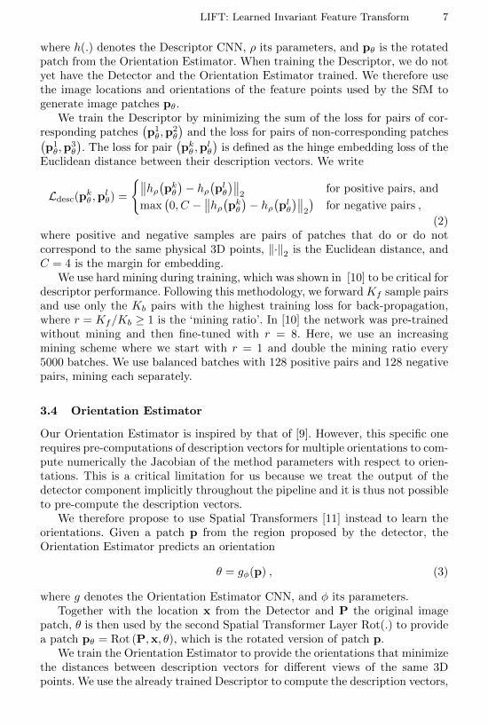
where h(.) denotes the Descriptor CNN, ρ its parameters, and pθ is the rotatedpatch from the Orientation Estimator. When training the Descriptor, we do notyet have the Detector and the Orientation Estimator trained. We therefore usethe image locations and orientations of the feature points used by the SfM togenerate image patches pθ.

We train the Descriptor by minimizing the sum of the loss for pairs of cor-responding patches

(p1θ,p

2θ

)and the loss for pairs of non-corresponding patches(

p1θ,p

3θ

). The loss for pair

(pkθ ,p

lθ

)is defined as the hinge embedding loss of the

Euclidean distance between their description vectors. We write

Ldesc(pkθ ,plθ) =

{∥∥hρ(pkθ)− hρ(plθ)∥∥2for positive pairs, and

max(0, C −

∥∥hρ(pkθ)− hρ(plθ)∥∥2

)for negative pairs ,

(2)where positive and negative samples are pairs of patches that do or do notcorrespond to the same physical 3D points, ‖·‖2 is the Euclidean distance, andC = 4 is the margin for embedding.

We use hard mining during training, which was shown in [10] to be critical fordescriptor performance. Following this methodology, we forward Kf sample pairsand use only the Kb pairs with the highest training loss for back-propagation,where r = Kf/Kb ≥ 1 is the ‘mining ratio’. In [10] the network was pre-trainedwithout mining and then fine-tuned with r = 8. Here, we use an increasingmining scheme where we start with r = 1 and double the mining ratio every5000 batches. We use balanced batches with 128 positive pairs and 128 negativepairs, mining each separately.

3.4 Orientation Estimator

Our Orientation Estimator is inspired by that of [9]. However, this specific onerequires pre-computations of description vectors for multiple orientations to com-pute numerically the Jacobian of the method parameters with respect to orien-tations. This is a critical limitation for us because we treat the output of thedetector component implicitly throughout the pipeline and it is thus not possibleto pre-compute the description vectors.

We therefore propose to use Spatial Transformers [11] instead to learn theorientations. Given a patch p from the region proposed by the detector, theOrientation Estimator predicts an orientation

θ = gφ(p) , (3)

where g denotes the Orientation Estimator CNN, and φ its parameters.Together with the location x from the Detector and P the original image

patch, θ is then used by the second Spatial Transformer Layer Rot(.) to providea patch pθ = Rot (P,x, θ), which is the rotated version of patch p.

We train the Orientation Estimator to provide the orientations that minimizethe distances between description vectors for different views of the same 3Dpoints. We use the already trained Descriptor to compute the description vectors,


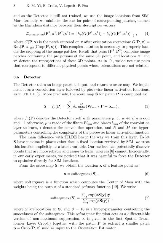
and as the Detector is still not trained, we use the image locations from SfM.More formally, we minimize the loss for pairs of corresponding patches, definedas the Euclidean distance between their description vectors

Lorientation(P1,x1,P2,x2) =∥∥hρ(G(P1,x1))− hρ(G(P2,x2))

∥∥2, (4)

where G(P,x) is the patch centered on x after orientation correction: G(P,x) =Rot(P,x, gφ(Crop(P,x))). This complex notation is necessary to properly han-dle the cropping of the image patches. Recall that pairs (P1,P2) comprise imagepatches containing the projections of the same 3D point, and locations x1 andx2 denote the reprojections of these 3D points. As in [9], we do not use pairsthat correspond to different physical points whose orientations are not related.

3.5 Detector

The Detector takes an image patch as input, and returns a score map. We imple-ment it as a convolution layer followed by piecewise linear activation functions,as in TILDE [6]. More precisely, the score map S for patch P is computed as:

S = fµ(P) =

N∑n

δnM

maxm

(Wmn ∗P + bmn) , (5)

where fµ(P) denotes the Detector itself with parameters µ, δn is +1 if n is oddand −1 otherwise, µ is made of the filters Wmn and biases bmn of the convolutionlayer to learn, ∗ denotes the convolution operation, and N and M are hyper-parameters controlling the complexity of the piecewise linear activation function.

The main difference with TILDE lies in the way we train this layer. To letS have maxima in places other than a fixed location retrieved by SfM, we treatthis location implicitly, as a latent variable. Our method can potentially discoverpoints that are more reliable and easier to learn, whereas [6] cannot. Incidentally,in our early experiments, we noticed that it was harmful to force the Detectorto optimize directly for SfM locations.

From the score map S, we obtain the location x of a feature point as

x = softargmax (S) , (6)

where softargmax is a function which computes the Center of Mass with theweights being the output of a standard softmax function [12]. We write

softargmax (S) =

∑y exp(βS(y))y∑y exp(βS(y))

, (7)

where y are locations in S, and β = 10 is a hyper-parameter controlling thesmoothness of the softargmax. This softargmax function acts as a differentiableversion of non-maximum suppression. x is given to the first Spatial Trans-former Layer Crop(.) together with the patch P to extract a smaller patchp = Crop (P,x) used as input to the Orientation Estimator.


As the Orientation Estimator and the Descriptor have been learned by thispoint, we can train the Detector given the full pipeline. To optimize over theparameters µ, we minimize the distances between description vectors for thepairs of patches that correspond to the same physical points, while maximizingthe classification score for patches not corresponding to the same physical points.

More exactly, given training quadruplets(P1,P2,P3,P4

), where P1 and P2

correspond to the same physical point, P1 and P3 correspond to different SfMpoints, and P4 to a non-feature point location, we minimize the sum of theirloss functions

Ldetector(P1,P2,P3,P4) = γLclass(P1,P2,P3,P4) + Lpair(P1,P2) , (8)

where γ is a hyper-parameter balancing the two terms in this summation

Lclass(P1,P2,P3,P4) =

4∑i=1

αi max(0,(1− softmax

(fµ(Pi))yi))2

, (9)

with yi = −1 and αi = 3/6 if i = 4, and yi = +1 and αi = 1/6 otherwise tobalance the positives and negatives. softmax is the log-mean-exponential softmaxfunction. We write

Lpair(P1,P2) = ‖ hρ(G(P1, softargmax(fµ(P1)))) −

hρ(G(P2, softargmax(fµ(P2)))) ‖2 .(10)

Note that the locations of the detected feature points x appear only implicitlyand are discovered during training. Furthermore, all three components are tiedin with the Detector learning. As with the Descriptor we use a hard miningstrategy, in this case with a fixed mining ratio of r = 4.

In practice, as the Descriptor already learns some invariance, it can be hardfor the Detector to find new points to learn implicitly. To let the Detector startwith an idea of the regions it should find, we first constrain the patch proposalsp = Crop(P, softargmax(fµ(P))) that correspond to the same physical pointsto overlap. We then continue training the Detector without this constraint.

Specifically, when pre-training the Detector, we replace Lpair in Eq. (8) with

Lpair, where Lpair is equal to 0 when the patch proposals overlap exactly, andincreases with the distance between them otherwise. We therefore write

Lpair(P1,P2) = 1− p1 ∩ p2

p1 ∪ p2+

max(0,∥∥x1 − x2

∥∥1− 2s

)√p1 ∪ p2

, (11)

where xj = softargmax(fµ(Pj)), pj = Crop(Pj ,xj), ‖·‖1 is the l1 norm. Recallthat s = 64 pixels is the width and height of the patch proposals.

3.6 Runtime pipeline

The pipeline used at run-time is shown in Fig. 4. As our method is trained onpatches, simply applying it over the image would require the network to be tested


SCALE-SPACE IMAGE SCORE PYRAMID

DET NMS

KEYPOINTS

Crop

RotORI… … DESC

d1

d2…

Scale-space Detection

dN

Fig. 4. An overview of our runtime architecture. As the Orientation Estimator and theDescriptor only require evaluation at local maxima, we decouple the Detector and run itin scale space with traditional NMS to obtain proposals for the two other components.

with a sliding window scheme over the whole image. In practice, this would betoo expensive. Fortunately, as the Orientation Estimator and the Descriptor onlyneed to be run at local maxima, we can simply decouple the detector from therest to apply it to the full image, and replace the softargmax function by NMS,as outlined in red in Fig. 4. We then apply the Orientation Estimator and theDescriptor only to the patches centered on local maxima.

More exactly, we apply the Detector independently to the image at differentresolutions to obtain score maps in scale space. We then apply a traditional NMSscheme similar to that of [1] to detect feature point locations.

4 Experimental validation

In this section, we first present the datasets and metrics we used. We then presentqualitative results, followed by a thorough quantitative comparison against anumber of state-of-the-art baselines, which we consistently outperform.

Finally, to better understand what elements of our approach most contributeto this result, we study the importance of the pre-training of the Detector com-ponent, discussed in Section 3.5, and analyze the performance gains attributableto each component.

4.1 Dataset and Experimental Setup

We evaluate our pipeline on three standard datasets:

– The Strecha dataset [33], which contains 19 images of two scenes seen fromincreasingly different viewpoints.

– The DTU dataset [34], which contains 60 sequences of objects with differentviewpoints and illumination settings. We use this dataset to evaluate ourmethod under viewpoint changes.

– The Webcam dataset [6], which contains 710 images of 6 scenes with strongillumination changes but seen from the same viewpoint. We use this datasetto evaluate our method under natural illumination changes.


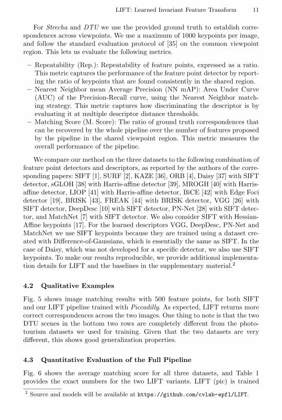
For Strecha and DTU we use the provided ground truth to establish corre-spondences across viewpoints. We use a maximum of 1000 keypoints per image,and follow the standard evaluation protocol of [35] on the common viewpointregion. This lets us evaluate the following metrics.

– Repeatability (Rep.): Repeatability of feature points, expressed as a ratio.This metric captures the performance of the feature point detector by report-ing the ratio of keypoints that are found consistently in the shared region.

– Nearest Neighbor mean Average Precision (NN mAP): Area Under Curve(AUC) of the Precision-Recall curve, using the Nearest Neighbor match-ing strategy. This metric captures how discriminating the descriptor is byevaluating it at multiple descriptor distance thresholds.

– Matching Score (M. Score): The ratio of ground truth correspondences thatcan be recovered by the whole pipeline over the number of features proposedby the pipeline in the shared viewpoint region. This metric measures theoverall performance of the pipeline.

We compare our method on the three datasets to the following combination offeature point detectors and descriptors, as reported by the authors of the corre-sponding papers: SIFT [1], SURF [2], KAZE [36], ORB [4], Daisy [37] with SIFTdetector, sGLOH [38] with Harris-affine detector [39], MROGH [40] with Harris-affine detector, LIOP [41] with Harris-affine detector, BiCE [42] with Edge Focidetector [19], BRISK [43], FREAK [44] with BRISK detector, VGG [26] withSIFT detector, DeepDesc [10] with SIFT detector, PN-Net [28] with SIFT detec-tor, and MatchNet [7] with SIFT detector. We also consider SIFT with Hessian-Affine keypoints [17]. For the learned descriptors VGG, DeepDesc, PN-Net andMatchNet we use SIFT keypoints because they are trained using a dataset cre-ated with Difference-of-Gaussians, which is essentially the same as SIFT. In thecase of Daisy, which was not developed for a specific detector, we also use SIFTkeypoints. To make our results reproducible, we provide additional implementa-tion details for LIFT and the baselines in the supplementary material.2

4.2 Qualitative Examples

Fig. 5 shows image matching results with 500 feature points, for both SIFTand our LIFT pipeline trained with Piccadilly. As expected, LIFT returns morecorrect correspondences across the two images. One thing to note is that the twoDTU scenes in the bottom two rows are completely different from the photo-tourism datasets we used for training. Given that the two datasets are verydifferent, this shows good generalization properties.

4.3 Quantitative Evaluation of the Full Pipeline

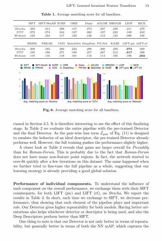
Fig. 6 shows the average matching score for all three datasets, and Table 1provides the exact numbers for the two LIFT variants. LIFT (pic) is trained

2 Source and models will be available at https://github.com/cvlab-epfl/LIFT.

https://github.com/cvlab-epfl/LIFT


Fig. 5. Qualitative local feature matching examples of left: SIFT and right: ourmethod LIFT. Correct matches recovered by each method are shown in green lines andthe descriptor support regions with red circles. Top row: Herz-Jesu-P8 of Strecha,second row: Frankfurt of Webcam, third row: Scene 7 of DTU and bottom row:Scene 19 of DTU. Note that the images are very different from one another.

with Piccadilly and LIFT (rf) with Roman-Forum. Both of our learned modelssignificantly outperform the state-of-the-art on Strecha and DTU and achievestate-of-the-art on Webcam. Note that KAZE, which is the best performingcompetitor on Webcam, performs poorly on the other two datasets. As discussedabove, Piccadilly and Roman-Forum are very different from the datasets usedfor testing. This underlines the strong generalization capability of our approach,which is not always in evidence with learning-based methods.

Interestingly, on DTU, SIFT is still the best performing method among thecompetitors, even compared to methods that rely on Deep Learning, such asDeepDesc and PN-Net. Also, the gap between SIFT and the learning-basedVGG, DeepDesc, and PN-Net is not large for the Strecha dataset.

These results show that although a component may outperform anothermethod when evaluated individually, they may fail to deliver their full potentialwhen integrated into the full pipeline, which is what really matters. In otherwords, it is important to learn the components together, as we do, and to con-sider the whole pipeline when evaluating feature point detectors and descriptors.

4.4 Performance of Individual Components

Fine-tuning the Detector. Recall that we pre-train the detector and thenfinalize the training with the Orientation Estimator and the Descriptor, as dis-


Table 1. Average matching score for all baselines.

SIFT SIFT-HesAff SURF ORB Daisy sGLOH MROGH LIOP BiCE

Strecha .283 .314 .208 .157 .272 .207 .239 .211 .270

DTU .272 .274 .244 .127 .262 .187 .223 .189 .242

Webcam .128 .164 .117 .120 .120 .113 .125 .086 .166

BRISK FREAK VGG MatchNet DeepDesc PN-Net KAZE LIFT-pic LIFT-rf

Strecha .208 .183 .300 .223 .298 .300 .250 .374 .369

DTU .193 .186 .271 .198 .257 .267 .213 .317 .308

Webcam .118 .116 .118 .101 .116 .114 .195 .196 .202

0

0.1

0.2

0.3

0.4

Avg. matching score on ‘Strecha’

SIFT SIFT-HesAf SURF ORB Daisy sGLOH MROGH LIOP BiCEBRISK FREAK VGG DeepDesc PN-Net MatchNet KAZE LIFT (pic) LIFT (rf)

0

0.1

0.2

0.3

0.4

Avg. matching score on ‘Strecha’0

0.08

0.16

0.24

0.32

Avg. matching score on ‘DTU’0

0.055

0.11

0.165

0.22

Avg. matching score on ‘Webcam’

Fig. 6. Average matching score for all baselines.

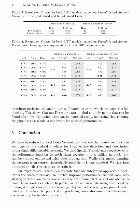
cussed in Section 3.5. It is therefore interesting to see the effect of this finalizingstage. In Table 2 we evaluate the entire pipeline with the pre-trained Detectorand the final Detector. As the pair-wise loss term Lpair of Eq. (11) is designedto emulate the behavior of an ideal descriptor, the pre-trained Detector alreadyperforms well. However, the full training pushes the performance slightly higher.

A closer look at Table 2 reveals that gains are larger overall for Piccadillythan for Roman-Forum. This is probably due to the fact that Roman-Forumdoes not have many non-feature point regions. In fact, the network started toover-fit quickly after a few iterations on this dataset. The same happened whenwe further tried to fine-tune the full pipeline as a whole, suggesting that ourlearning strategy is already providing a good global solution.

Performance of individual components. To understand the influence ofeach component on the overall performance, we exchange them with their SIFTcounterparts, for both LIFT (pic) and LIFT (rf), on Strecha. We report theresults in Table 3. In short, each time we exchange to SIFT, we decrease per-formance, thus showing that each element of the pipeline plays and importantrole. Our Detector gives higher repeatability for both models. Having better ori-entations also helps whichever detector or descriptor is being used, and also theDeep Descriptors perform better than SIFT.

One thing to note is that our Detector is not only better in terms of repeata-bility, but generally better in terms of both the NN mAP, which captures the


Table 2. Results on Strecha for both LIFT models trained on Piccadilly and Roman-Forum, with the pre-trained and fully-trained Detector.

Trained on Piccadilly Trained on Roman-Forum

Rep. M.Score Rep. M.ScorePre-trained .436 .367 .447 .368

Fully-trained .446 .374 .447 .369

Table 3. Results on Strecha for both LIFT models trained on Piccadilly and Roman-Forum, interchanging our components with their SIFT counterparts.

Trained on Piccadilly Trained on Roman-Forum

Det. Ori. Desc. Rep. NN mAP M.Score Rep. NN mAP M.Score

SIFT SIFT SIFT

.428

.517 .282

.428

.517 .282

SIFT Ours SIFT .671 .341 .662 .338

SIFT SIFT Ours .568 .290 .581 .295

SIFT Ours Ours .685 .344 .688 .342

Ours SIFT SIFT

.446

.540 .325

.447

.545 .319

Ours Ours SIFT .644 .372 .630 .360

Ours SIFT Ours .629 .339 .644 .337

Ours Ours Ours .446 .686 .374 .447 .683 .369

descriptor performance, and in terms of matching score, which evaluates the fullpipeline. This shows that our Detector learns to find not only points that can befound often but also points that can be matched easily, indicating that trainingthe pipeline as a whole is important for optimal performance.

5 Conclusion

We have introduced a novel Deep Network architecture that combines the threecomponents of standard pipelines for local feature detection and descriptioninto a single differentiable network. We used Spatial Transformers together withthe softargmax function to mesh them together into a unified network thatcan be trained end-to-end with back-propagation. While this makes learningthe network from scratch theoretically possible, it is not practical. We thereforeproposed an effective strategy to train it.

Our experimental results demonstrate that our integrated approach outper-forms the state-of-the-art. To further improve performance, we will look intostrategies that allow us to take advantage even more effectively of our ability totrain the network as a whole. In particular, we will look into using hard negativemining strategies over the whole image [45] instead of relying on pre-extractedpatches. This has the potential of producing more discriminative filters and,consequently, better descriptors.


References

1. Lowe, D.: Distinctive Image Features from Scale-Invariant Keypoints. IJCV 20(2)(2004)

2. Bay, H., Ess, A., Tuytelaars, T., Van Gool, L.: SURF: Speeded Up Robust Features.CVIU 10(3) (2008) 346–359

3. Tola, E., Lepetit, V., Fua, P.: A Fast Local Descriptor for Dense Matching. In:CVPR. (2008)

4. Rublee, E., Rabaud, V., Konolidge, K., Bradski, G.: ORB: An Efficient Alternativeto SIFT or SURF. In: ICCV. (2011)

5. Mainali, P., Lafruit, G., Tack, K., Van Gool, L., Lauwereins, R.: Derivative-BasedScale Invariant Image Feature Detector with Error Resilience. TIP 23(5) (2014)2380–2391

6. Verdie, Y., Yi, K.M., Fua, P., Lepetit, V.: TILDE: A Temporally Invariant LearnedDEtector. In: CVPR. (2015)

7. Han, X., Leung, T., Jia, Y., Sukthankar, R., Berg, A.C.: MatchNet: UnifyingFeature and Metric Learning for Patch-Based Matching. In: CVPR. (2015)

8. Zagoruyko, S., Komodakis, N.: Learning to Compare Image Patches via Convolu-tional Neural Networks. In: CVPR. (2015)

9. Yi, K., Verdie, Y., Lepetit, V., Fua, P.: Learning to Assign Orientations to FeaturePoints. In: CVPR. (2016)

10. Simo-Serra, E., Trulls, E., Ferraz, L., Kokkinos, I., Fua, P., Moreno-Noguer, F.:Discriminative Learning of Deep Convolutional Feature Point Descriptors. In:ICCV. (2015)

11. Jaderberg, M., Simonyan, K., Zisserman, A., Kavukcuoglu, K.: Spatial TransformerNetworks. In: NIPS. (2015)

12. Chapelle, O., Wu, M.: Gradient Descent Optimization of Smoothed InformationRetrieval Metrics. Information Retrieval 13(3) (2009) 216–235

13. Harris, C., Stephens, M.: A Combined Corner and Edge Detector. In: FourthAlvey Vision Conference. (1988)

14. Moravec, H.: Obstacle Avoidance and Navigation in the Real World by a SeeingRobot Rover. In: tech. report CMU-RI-TR-80-03, Robotics Institute, CarnegieMellon University, Stanford University. (September 1980)

15. Rosten, E., Drummond, T.: Machine Learning for High-Speed Corner Detection.In: ECCV. (2006)

16. Matas, J., Chum, O., Martin, U., Pajdla, T.: Robust Wide Baseline Stereo fromMaximally Stable Extremal Regions. In: BMVC. (September 2002) 384–393

17. Mikolajczyk, K., Schmid, C.: An Affine Invariant Interest Point Detector. In:ECCV. (2002) 128–142

18. Forstner, W., Dickscheid, T., Schindler, F.: Detecting Interpretable and AccurateScale-Invariant Keypoints. In: ICCV. (September 2009)

19. Zitnick, C., Ramnath, K.: Edge Foci Interest Points. In: ICCV. (2011)

20. Mainali, P., Lafruit, G., Yang, Q., Geelen, B., Van Gool, L., Lauwereins, R.: SIFER:Scale-Invariant Feature Detector with Error Resilience. IJCV 104(2) (2013) 172–197

21. Sochman, J., Matas, J.: Learning a Fast Emulator of a Binary Decision Process.In: ACCV. (2007) 236–245

22. Trujillo, L., Olague, G.: Using Evolution to Learn How to Perform Interest PointDetection. In: ICPR. (2006) 211–214


23. Strecha, C., Bronstein, A., Bronstein, M., Fua, P.: LDAHash: Improved Matchingwith Smaller Descriptors. PAMI 34(1) (January 2012)

24. Winder, S., Brown, M.: Learning Local Image Descriptors. In: CVPR. (June 2007)25. Perez, C., Olague, G.: Genetic Programming As Strategy for Learning Image

Descriptor Operators. Intelligent Data Analysis 17 (2013) 561–58326. Simonyan, K., Vedaldi, A., Zisserman, A.: Learning Local Feature Descriptors

Using Convex Optimisation. PAMI (2014)27. Zbontar, J., LeCun, Y.: Computing the Stereo Matching Cost with a Convolutional

Neural Network. In: CVPR. (2015)28. Balntas, V., Johns, E., Tang, L., Mikolajczyk, K.: PN-Net: Conjoined Triple Deep

Network for Learning Local Image Descriptors. In: arXiv Preprint. (2016)29. Wilson, K., Snavely, N.: Robust Global Translations with 1DSfM. In: ECCV.

(2014)30. Wu, C.: Towards Linear-Time Incremental Structure from Motion. In: 3DV. (2013)31. Paulin, M., Douze, M., Harchaoui, Z., Mairal, J., Perronnin, F., Schmid, C.: Local

Convolutional Features with Unsupervised Training for Image Retrieval. In: ICCV.(2015)

32. Sermanet, P., Chintala, S., LeCun, Y.: Convolutional Neural Networks Applied toHouse Numbers Digit Classification. In: ICPR. (2012)

33. Strecha, C., Hansen, W., Van Gool, L., Fua, P., Thoennessen, U.: On Benchmark-ing Camera Calibration and Multi-View Stereo for High Resolution Imagery. In:CVPR. (2008)

34. Aanaes, H., Dahl, A.L., Pedersen, K.S.: Interesting Interest Points. IJCV 97 (2012)18–35

35. Mikolajczyk, K., Schmid, C.: A Performance Evaluation of Local Descriptors. In:CVPR. (June 2003) 257–263

36. Alcantarilla, P., Fernandez, P., Bartoli, A., Davidson, A.J.: KAZE Features. In:ECCV. (2012)

37. Tola, E., Lepetit, V., Fua, P.: Daisy: An Efficient Dense Descriptor Applied toWide Baseline Stereo. PAMI 32(5) (2010) 815–830

38. Bellavia, F., Tegolo, D.: Improving Sift-Based Descriptors Stability to Rotations.In: ICPR. (2010)

39. Mikolajczyk, K., Schmid, C.: Scale and Affine Invariant Interest Point Detectors.IJCV 60 (2004) 63–86

40. Fan, B., Wu, F., Hu, Z.: Aggregating Gradient Distributions into Intensity Orders:A Novel Local Image Descriptor. In: CVPR. (2011)

41. Wang, Z., Fan, B., Wu, F.: Local Intensity Order Pattern for Feature Description.In: ICCV. (2011)

42. Zitnick, C.: Binary Coherent Edge Descriptors. In: ECCV. (2010)43. Leutenegger, S., Chli, M., Siegwart, R.: BRISK: Binary Robust Invariant Scalable

Keypoints. In: ICCV. (2011)44. Alahi, A., Ortiz, R., Vandergheynst, P.: FREAK: Fast Retina Keypoint. In: CVPR.

(2012)45. Felzenszwalb, P., Girshick, R., McAllester, D., Ramanan, D.: Object Detection

with Discriminatively Trained Part Based Models. PAMI (2010)

lift: learned invariant feature transform arxiv:1603 ... · pdf filelift: learned invariant...

Documents