light interception, growth dynamics, and dry matter ... interception, growth dynamics, and dry...
TRANSCRIPT
...;
...
•
Light Interception, Growth Dynamics, and Dry Matter Partitioning in aPhytotron-grown Snap Bean (Phaseolus vUl~aris L.) Crop:
A Modeling Analysis with Reference to Airol1ution Effects.
JOHANN HEINRICH LIETH
Biomathematics Series No. 11Institute of Statistics Mimeo Series No. 1620North Carolina State University, Raleigh, NC 1982
NORTH CAROLINA STATE UNIVERSITYRaleigh, North Carolina

-e LIGHT INTERCEPTION. GROWTH DYNAMICS, AND DRY MATTER PARTITIONING
IN A PHYrOTRON-GROWN SNAP -BEAN (Phaseolus vulgaris ,h) CROP:
A MODELING ANALYSIS WITH REFERENCE TO AIR POLLUTION EFFECTS
by
Johann Heinrich Lieth
A thesis submitted to the Graduate Faculty ofNorth Carolina State Universityin partial fulfillment of the
requirements for the Degree ofDoctor of Philosophy
BIOMATHEMATICS PROGRAM
DEPARTMENT OF STATISTICS
RALEIGH
1 982
APPROVED BY:
Co-Chairman of Advisory Committee Co-Chairman of Advisory Committee
-eABSTRACT
LIETH, JOHANN HEINRICH. Light Interception, Growth Dynamics, and Dry·
Matter Partitioning in a Phytotron-grown Snap Bean (Phaseolus vullaris
L.) Crop: A Modeling Analysis with Reference to Air Pollution Effects.
(Under the direction of JAMES F. REYNOLDS)
The development of a plant growth model for snap bean (Phaseolus
vulgaris L.) was conducted as four separate projects: 1) analysis of
canopy light interception, 2) a plant growth analysis of episodic
events, 3) a theoretical development of a plant growth simulation
model, and 4) application of the simulation model to the cultivar 'Bush
Blue Lake 290'. Each project is treated separately within this
dissertation:
1) Simple exponential decay models were used to describe the
variation in ir~adiance within a snap bean canopy over a 33-day period.
Extinction coefficients were varied over time as a function of total
leaf area and/or canopy height, and nonlinear least squares procedures
were used to estimate parameter values. An index was defined to assess
the applicability of these models for use in whole-plant simulation .
models.
2) A technique was developed for analyzing plant growth where
short-term stress (such as gaseous air pollution exposure) occurs during
plant ontogeny resulting in a discontinuous growth rate. The method,
based on the Richards growth function was applied to growth data of snap
bean exposed to ozone. The technique was investigated for episodic and
multi-episodic events.
3) A carbon-allocation simulation model for the growth of snap
bean, consisting of a set of recursive equations with a daily time step,

-e simulating lea~, stem, root, and reproductive dry weights over a six
week. period, was developed.
Various submodels were incorporated: leaf photosynthesis,
whole-plant respiration, partitioning of assimilates, and canopy
structure. The design of the model, through its emphasis on foliage
structure, provides a detailed representation of the canopy growth
dynamics. Potential extensions and applications of the model are
discussed.
4) The model was applied to the variety 'Bush Blue Lake 290'.
Parameters were estimated from both experimental and published data.
The resulting simulation was compared to the parameter data set as well
as a validation data set. The model behavior appeared to be
satisfactory over the range of environmental conditions used. Further
model development is discussed specifically with respect to air
pollutant effects.

BIOGRAPHY ii
-e The author was born in Cologne, West Germany on January 2, 1955.
He attended German elementary schools until his family's emigration
the United States in December 1966 where he attended junior and senior
high schools until his graduation in 1972.
From May 1972 to May 1976, the author attended the University of
North Carolina at Chapel Hill where he received a Bachelor of Science
degree in Mathematical Sciences. Upon graduation, he attended NOrth
Carolina State University, culminating in a Master of Science degree
in Applied Mathematics in May 1978, at which time he was accepted into
the Biomathematics Program.
During the summers between the academic years 1970 to 1980, the
author has, when not attending summer school, worked in many diverse
positions ranging from construc~ion work to chemistry laboratory assis
tant at a nuclear research facility. He has held jobs as accountant
assistant to a computing center, mycology laboratory assistant, as well
as holding an internship with the North Carolina State Government.
The author is married to the former Sharyn Elizabeth O'Neil of
Winston-Salem. Mrs. Lieth graduated from UNC-Chapel Hill with a
bachelor's degree in Early Childhood Education in May 1980 and is
presently teaching at lmmaculata Elementary School in Durham, North
Carolina.

TABLE OF CONTENTSiii
-e PREFACE • • • • • • • • • • • • • • • • • • • • • • • • • • • •
Page
1
I. LIGHT INTERCEPTION BY A DEVELOPING SNAP BEAN CANOPY • • • • 5
ABSTRACT •••••••• • • • • • • • • • • • • • • • •• 6INTRODUcrION • • • • • • • • • • •.• • • • • • • • • • •• 7METHODS AND MATERIALS • • • • • • • • • • • • • • • • • •• 8
Model Development • • • • • • • • • • • • • • • • • •• 8Experimental Data • • • • • • • • • • • • • • • • • •• 13
RESULTS AND DISCUSSION • • • • • • • • • • • • • • • • •• 16CONCLUSION • • • • • • • • • • • • • • • • • • • • • • •• 23REFERENCES ••••• • • • • • • • • • • • • • • • • • •• 25
II. PLANT GROWTH ANALYSIS: A METHOD FOR QUANTIFYING THE EFFEcrSOF EPISODIC AIR POLLtrrION STRESS ON PLANT GROWTH •• • •
ABSTRAcr • • • • • • • • • • • • • • • • • • • • • • • • •INTRODUCTION •• • • • • • • • • • • • • • • • • • • • • •METHODS AND MATERIALS • • • • • • • • • • • • • • • • • • •
Experimental Design • • • • • • • • • • • • • • • • • •Fitting Strategies • • • • • • • • • • • • • • • • • •
RESULTS AND DIScUSSION • • • • • • • • • • • • • • • • • •~y ••••••••••••••••••••••••••REP'ERENCES •••••• • • • • • • • • • • • • • • • • •
272829353537384748
ABSTRACT • • • • • • • • • • • • • • • • • • • • • • • • • •INTRODUCTION • • • • • • • • • • • • • • • • • • • • • • • •MODEL STRUCTURE ••• • • • • • • • • • • • • • • • • • • •
Ir rad iance • • • • • • • • • • • • • • • • • • • • • • • •Leaf Photosynthesis •••••••••••••••••••Respiration •• • • • • • • • • • • • • • • • • • • • • •Allocation • • • • • •• ••••••••••••••••Canopy Characteristics • • • • • • • • • • • • • • • • • •
DISCUSSION • • • • • • • • • • • • • • • • • • • • • • • • •REFERENCES • • • • • • • • • • • • • • • • • • • • • • • • •
III. A PLANT GROWTH MODEL FOR SNAP BEAN: I. THEORY •• • • • • • 4950515254565960616366
6970717277777892939494
102104
• • •• • • •• • • •
APPLICATION TOLAKE 290' GROWN UNDER
• • • • • • •
A PLANT GROWTH MODEL FOR SNAP BEAN: II.PHASEOLUS VULGARIS L. CV. 'BUSH BLUECONTROLLED CONDITIONS
ABSTRACT • • • • • • • • • • • • • • • • • • • • • • • • • •INTRODUCTION • • • • • • • • • • • • • • • • • • • • • • • •MODEL OVERVIEW • • • • • • • • • • • • • • • • • • • • • • •METHODS AND MATERIALS •••••••••••••• • • • • •
Experimental Design • • • • • • • • • • • • • • • • • • •Determination of Model Parameters and ConstantsModel Adjustments ••••••••••••••••••••Programming Considerations • • • • • • • • • • • • • • • •
RESULTS AND DISCUSSION • • • • • • • • • • • • • • • • • • •Model Behavior • • • • • • • • • • • • • • • • • • • • • •Validation • • • • • • • • • • • • • • • • • • .'. • • • •Recommendations for Future Work •• • • • • • • • • • • •
IV.

iv
CONCLUSION" • • • • • • • • • • • • • •REFERENCES • • • • • • • • • • • • •
APPENDIX A: LEAF IDENTIFICATION SCHEME
· . . . . . . . .
· . . . . ...111"112
115
117117
118120
. . .· . .
APPENDIX B: DETERMINATION OF PHOTOSYNTHETIC PARAMETERV.ALtJES • • • • • • • • • • • • • • • • • • •Determination of at P , and R- • • • • • •n,max -1.Determination of a . • • . • • . •Exa.mple .•••••.. • . . . • .
APPENDIX C: BEAN: PL!I COMPUTER PROGRAM AND NOTES •• 124

PUF~E
This modeling study was started in 1980 in cooperation with the
Agricultural Research Service of the United States Department of
Agriculture* with the goal to develop modeling tools for use in their
air pollution research activities. These activities span various types
of pollutants (03, S02' N02), alone" and in combination, in
various doses (acute and chronic), in the phytotron, greenhouse and
field. Since this presents an enormous base for model application, a
project was drawn up, as a subset of the whole, restricted to episodic
exposures of ozone on plants grown in the phytotron.
In February of 1981, I went to the Glasshouse Crops Research
Institute in Littlehampton, England for one month to develop with the
aid of Dr. James Reynolds, an extensive outline of the modeling
objectives and possible results, together with the necessary
experimental design. The objective of the work was to investigate the
canopy architecture, leaf CO2 exchaDge photosynthesis, and plant
part fresh and dry weight distribution for snap bean plants exposed to
various levels of ozone. This project was seen as slightly
overambitious and was thus trimmed to exclude the photosynthesis work.
Actual experimentation was done between May and Septeaber of 1981.
The model developed in the last two chapters (III and IV) of this thesis
was built on the data fram the control plants of these experiments.
*USDA/ARS Cooperative Agreement with the North Carolina
Agricultural Research Service - Number: 12-14-7001-1140.

2
The light measurements provided some interesting ideas and insights
into the distribution of photosynthetically active radiation in a
developing snap bean canopy. This is written up as Chapter I.
While analyzing the data for ozone effects using modern techniques
of plant growth analysis, an interesting discovery was made: It is
possible, through modification of the differential equation underlying
the applied growth function, to directly estimate specific quantities
which were heretofore not measurable. In the case of episodic ozone
stress, this included the percent reduction in the growth rate at the
time of the event, and the rate of recovery of the growth rate. Since
this presents a powerful new tool, it is also written up separately
(Chapter II), together with ideas on how to extend the technique to
other types of situations where growth is affected.
A large array of possibilities for future projects resulted frOB
this work:
1.) Design and carry out studies to validate the light
interception model under the fluctuating conditions presented in
greenhouses and field conditions.
2.) Determine whether light attenuation is affected by foliar
ozone damage (other than through the reduced plant size).
3.) Expand the growth analysis techniques presented in Chapter II
to illustrate a variety of different effects (not just stress). Modify,
in particular, to study multiple episodic events (as illustrated) and
long-term chronic situations.
4.) Expand the growth analysis technique to other areas of the
life sciences. Investigate the application in demographic studies on
animals as well as plants. Its application to any growth process
characterizable with a growth function should be possible.
e-
3
5.) carry out a sensitivity analysis on the snap bean model
(Chapter III and IV, Apendix C). This needs to be done prior to further
model modifications.
6.) Carry out submodel validations, especially for the
photosynthesis and respiration submodels. This will involve collecting
CO2 exchange data for whole plants as well a8 individual leaves of
all ages for the range of light levels found in the canopy as well as
high light levels (saturation).
7.) Develop methods to allow the model in Chapter III and IV to be
utilized as a hypothesis testing tool in air pollution studies.
8.) Study the difference between field and phytotron conditions
and develop a method by which a phytotron-developed model can be
converted to incorporate field conditions.
All the work represented by this thesis could not have been done
without the cooperation of many individuals, especially the scientists
and staff of the Air Quality group of the ARS/USOA. The research
leader, Dr. Walter Heck, provided continued interest, support and
inspiration.
Foremost, however, I wish to express my sincerest appreciation to
Dr. James Reynolds for his guidance during the last three years. His
many efforts on my behalf, in the face of perpetual shortness of
available time, were a consistent inspiration to me. I also wish to
thank him and his family for their hospitality during my stay with them
in England.
Within the academic cOBmunity here at North carolina State
University many individuals have excerted a powerful influence on the
direction of my career. Dr. R. R. van der Vaart, through his excellent

4
lectures in Biomathematics, has been one of the main forces in my
decision to focus on this area within the field of applied mathematics~
Dr. Harvey Gold (the Biomathematic Program Chairman), Nancy Evans and
Ann Ethridge (the program secretaries), and my fellow BiOlllath graduate
students have made my tenure enjoyable.
I would also like to thank: Mr. John Dunning and Mrs. Joy Smith
for their guidance during the early phases of the experimentation, the
phytotron staff for their professional handling of my experiments, and
Dr. John Bishir for his help during my tenure in the Department of
Mathematics and his recent help with reviewing and critiquing my work.
I am also grateful to the Department of Statistics for their
support through their provision of office space and cOlllputer funds.
I am indebted to the typists at the Air Quality office for their
assistance with this thesis. I am especially grateful to Ms. Marcia
Bastian for her excellent typing of the text.
I would like to express my gratitude to my family for their support
and sacrifice. I am especially grateful to my parents who have
untiringly encouraged me for a quarter of century. I would also like to
thank my wife, Sharyn, who in the face of the prospect of spending the
rest of her life with a research scientist, married me anyway. Her help
and support with this thesis are also appreciated.
Heinrich Lieth
November 1982
-e
I
LIGHT INTERCEPTION BY A DEVELOPING SNAP BEAN CANOPY

6
ABSTRA<:r
Simple exponential decay models are used to describe the variation
in light attenuation within a snap bean (Phaseolus vulgaris L.) canopy
over a 33-day period of canopy development. Extinction coefficients are
varied over time as a function of (1) total leaf area and (2) canopy
height, and nonlinear least-squares procedures are used to estimate
parameter values for these models. The response surfaces generated to
depict changes in light attenuation accompanying canopy development
illustrate the dynamic nature of canopy closure. A criterion index is
defined to aid in assessing the applicability of these models for use in
whole-plant simulation models, and an evaluation of these models is
given based on this index, their predictive accuracy, and utility for
use within varying modeling frameworks.

7
INTRODUCTIOt-J
The development of a plant growth model at the community level
requires an understanding of the various interactions of the plant
canopy with its environment. In particular, the radiation regime within,
a canopy is of prime importance due to its role in photosynthesis,
transpiration, and its photomorphogenic effects on growth and
development (Ross, 1977). Consequently, a large number of light
attenuation models have been developed, ranging from simple exponential
decay (e.g., Monsi and Saeki, 1953) to complicated geometric
foraulations (e.g., Fuchs and Stanhill, 1980). Models have been
developed for isolated plants of varying geometries (e.g., Stamper and
Allen, 1979), for row crops with differing spatial distributions (e.g.,
Mann et al., 1982), of suu-flecking phenomena (e.g., Mann and Curry,
1977), of the statistical distribution of both leaf-aagles (e.g., Loomis
and Williams, 1969) and phytomatter (e.g., Ac:ock et al., 1970) within
canopies, etc. Comprehensive reviews are given by Monteith (1973),
Lemeur and Blad (1974), and Thornley (1976).
The adoption of any of the above formulations for use within a
dynamic simulation model of plant growth, however, poses a variety of
problems. Perhaps the most serious is that of compleXity. Rarely are
data available (for statistical-fitting purposes) commensurate with the
complexity of most of these models. In fact, Lemeur and Blad (1974)
state that due to the continual increase in the mathematical complexity
of radiation models in recent years, a thorough comprehension of these
models 1s usually limited to their authors alone. In addition, numerous
geometrical properties of a plant canopy (e.g., leaf areas, angles, and
and positions) change with phenological aging, and vary between species,

8
which makes the incorporation of such cOlllplex 1IlOdel structures within
the framework of a dynamic growth 1IlOdel unrealistic.
In this paper a silllple approach to modeling light attenuation
during the course of canopy development (days 5-38) in snap bean
(Phaseolus vulgaris L.) grown in a controlled environment facility is
presented. This model was designed for use as a submodel in a snap bean
growth s11llulator being developed to study ozone effects on crop growth
rates. The objective was to select a simple model structure that would
(1) utilize a readily attainable data base, (2) be easily applied to
different cultivars or species by straightforward reparameterization,
(3) provide a continuous representation of the light regime in a
developing crop canopy, and (4) maxilllize predictive accuracy subject to
constraints illlposed by objectives (1) - (3).
METHODS AND MATERIALS
Model Developlllent
The following model is based on Monteith's (1965) treatment of
light attenuation within a canopy that has been subdivided into unit
leaf area layers. It is assumed that direct and scattered light is
intercepted in the 881Ile way and that there is no overlap of leaves
within a layer. Letting s be the unintercepted fraction of incident
irradiation that passes through a layer and '! the mean leaf transmission
coefficient, the radiation intensity OJE 1Il-2 s-l) after F layers
have been penetrated is given by:
I(F) • 10 [s + (l-s)'!]F (1)
where 10 is the incident irradiance at the top of the canopy. If,
instead, the canopy is divided into layers of leaf area lin, resulting

9in nF layers, ~nd assuming a homogeneous leaf distribution, the
fractional area of intercepted light will change from (l-s) to (l-s)/n
and the fraction which passes through unintercepted will be (1-(1-s)!n).
Thus eqn (1) can be rewritten as:
I(nF) • 10 [(1- l::!.) + l::!. T ]nFn n
A continuous model is obtained in the limit as n approaches infinity
(Monteith, 1973):
I(F) • 10 lim [1 - .!:!. + .!:!.T.fFn~ . n n
• 10
lim [1 + -(1-s)( 1- 'T') ]nFn..c. n
-(1-S)(1-T)F• Ioe
Since Tand s are constants, we can set:
it • (1-s)( 1-"')
and eqn (3c) can be written as:
I(F) • 1oe-kF
Monsi and Saelti (1953) first applied such a model to crop canopies.
(3&)
(3b)
(3c)
. (4)
(5)
Wide use has been made of different versions of this model (see Lemeur
and Blad, 1974).
In eqn (5), F represents the total cumulative leaf-area (m2) above
a given depth into the canopy. In this paper we explore an alternative
form of eqn (5), namely:
I(X) • I e-kXo
where X is the linear depth (measured in meters) from the top of the
(6)
canopy. Both models require two assumptions: (1) a random distribution
of leaves and (2) a homogeneous leaf material distribution throughout
the canopy. The first assumption is needed in the derivation of the

10
discrete version [eqn (l)] and the second assumption is needed for the
continuous model [eqn (5)]. Technically, the latter cannot be achieved'
by a canopy of leaves since it implies a continuous medium of leaf
material; it can, however, be approximated fairly well by canopies
containing many small, randomly distributed leaves. Both assumptions
restrict the use of the models to closed canopies.
In order to use eqns (5)-(6) for predicting the radiation regime
within the canopy of a developing crop, the extinction coefficient,
k, must change as a function of the size and density of the canopy. Bow
k might be expected to vary can be examined by considering various
combinations of k, 'tot (total canopy leaf area), and the fraction of
incident light reaching the bottom of the canopy (see Fig. 1). In Fig.
2, values of k obtained by fitting eqn (S) to samples of snap bean ~
canopies sampled at 3-4 day intervals during the course of development
show declining values of k with total leaf area. These preliminary
results suggest that the use of equs (5)-(6) in a dynamic growth model
requires that k be represented by a function of some canopy
characteristic. In this analysis, a linear function of the fora
k - A + B·Ftot
and a hyperbolic function of the fora
k-A+..!Ftot
where A and B are parameters defining the shape of the curves, and
Ftot is total leaf area, were used in conjunction with eqn (5).
,Similarly,
k - A + B·B
and
k - A + BIB
(7)
(8)
(9)
e(IO)

11
k
8.IS 8.S 8.75 8.95
Figure 1. Plots of the curve k· -(log I/Io»/Ftot (solid lines),representing the relationship between the fraction of lightreaching the bottom of the canopy (IlIa) and the extinctioncoefficient for six values of the total leaf area (Ftot).The two trajectories (dashed lines) show how k may decrease(trajectory 1) or increase (trajectory 2) as the canopydevelops.

12
I
I
•
, .•
•, .
• ••
•••
•
,•
•
•
•
.'I
'"
•
•
I
•
•• I
•
I
•••
k
8 .84 .88 .12 .18 .29 .24
Tolal leal Area eft.>
Figure 2. Extinction coefficients, k, estimated by fitting the linearizedversion of eqn (5), log (IlIa) • -kF, and the corresponding R2(coefficient of determination) values, plotted against thetotal leaf area (Ftot) •

13
• where H is the height of the canopy, were used in conjunction with
eqn (6). Note that k is in units of m-2 in eqns (7)-(8) and in m-1
in eqns (9)-(10). This leads to the following four models:
I = Ioe-(A + B.Ftot)F
I • Ioe-(A + B/Ftot)F
I • Ioe-(A + B·H)X
I • Ioe-(A + B/H)X
Experimental Data
(11)
(12)
(13)
(14)
•
•
Selected canopy characteristics of snap bean plants (~ vulgaris
L. cv. "Bush Blue Lake 290") were measured during a 33-day period of
development. Plants were grown in 15.2 em diameter pots i~ walk-in
chambers of the Southeastern Plant Environment Laboratory (phytotron)
under controlled conditions: day lengths of 9 hours at 26 degrees C and
15 hour (uninterrupted) nights at 22 degrees C. Standard nutrient and
soil conditions for the facility were used (Downs and Bonaminio, 1976).
Nutrient solution was applied each morning and deionized water in the
·afternoon in sufficient quantities to drip through the pots. Light
quality during the day was kept uniform by maintaining a fixed
proportion of incandescent and fluorescent lights (Downs and Bonaminio,
1976) resulting in ca. 590 ~E m-2 s-1 at the top of the canopy.
Plants were grown at a density of ca. 24 plants m-2, surrounded
by a perimeter of plants to minimize edge effects. Following seedling
emergence, destructive harvests were made every 3 days from day 5
through 14 and every 4 days from day 18 to 38; at each harvest, 4 plants
were separated into leaf, stem, root, and reproductive organs for fresh
weight determinations. For each trifoliate leaflet and primary leaf,
leaf (leaflet) blade length, area and fresh weight were measured. Leaf
14
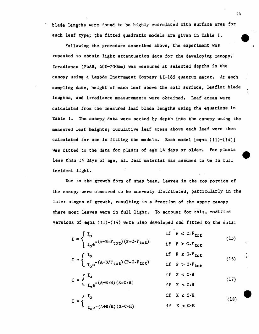
blade lengths were found to be highly correlated with surface area for
each leaf type;, the fitted quadratic models are given in Table 1•
Following the procedure described above, the experiment was
repeated to obtain light attentuation data for the developing canopy.
Irradiance (PhAR, 40o-70Onm) was measured at selected depths in 'the
canopy using a Lambda Instrument Company LI-185 quantum meter. At each
•sampling date, height of each leaf above the soil surface, leaflet blade
lengths, and irradiance measurements were obtained. Leaf areas were
calculated from the measured leaf blade lengths using the equations in
Table 1. The canopy data were sorted by depth into the canopy using the
measured leaf heights; cumulative leaf areas above each leaf were then
calculated for use in fitting the models. Each model [eqns (11)-(14)]
was fitted to the data for plants of age 14 days or older. For plants
less than 14 days of age, all leaf material was assumed to be in full
incident light.
Due to the growth form of snap bean, leaves in the top portion of
•the canopy were observed to be unevenly distributed, particularly in the
later stages of growth, resulting in a fraction of the upper canopy
where most leaves were in full light. To account for this, modified
versions of eqns (11)-(14) were also developed and fitted to the data:
={10
if F :s: C,FtotI I -(A+B.Ftot) (F-C.Ftot)
oe if F > C.F tot
={ 10 if F :s: C.FtotI Iee-(A+B/Ftot) (F-C.Ftot) if F > C·F tot
f Ie if X :s: C·R1= -(A+B.R) (X.C.R)Ioe if X > C·R
1= {Ie if X :s: C·R
Ioe-(A+B!H) (X.C.R) if X > C·R
(15)
(16)
(17)
(18) •

15
Table 1. Quadratic polynomials resulting from fitting leaf area(m2), A , against 1 eaf blade length (m), LJ,' Eituationswere fil without intercepts to guarantee ~"O for LJ,"O'The fittings were carried out on the 3 di erent typesof leaf material (primary leaves, trifoliate mid •leaflets, and trifoliate side leaflets) using a generallinear models routine.
Leaf Leaflet Equationtype type R2
Primary AJ, 2 0.761 *L 2 + 0.00886*Lt
.990:t
mid At 2 0 • 425*Ll - 0.OO333*Lt ·993Trifoliate
side At 2 0.499*L/ - 0.OO599*Lt ·993
•
•
•

•
•
•
16
where C is a model parameter representing the fraction of the upper
canopy in which all leaves are in full light.
All computing was done on the 'Triangle Universities Computer
Center IBM 3081 computer using the Statistical Analysis System (Helwig
and Council, 1979). The Marquardt method was used in the nonlinear
regressions. Computer graphics were generated using SAS/GRAPH (Council
and HelWig, 1981).
RESULTS AND DISCUSSION
The results of the nonlinear statistical fitting of the various
models are summarized in Table 2. The fitted values of B in the k
functions, i.e., negative in the linear models and positive in the
hyperbolic models, imply that k decreases with increased canopy size
(measured either by total leaf area or canopy height). To illustrate
the predictive response surface characterizing the light attenuation
through the canopy during the course of canopy development (days 5-38),
three-dimensional plots of the'simple [eqn (11), Table 2] and modified
[eqn (16), Table 2] leaf area versions of the models sre shown in
Fig. 3.
To evaluate the overall results summarized in Table 2, three points
related to each model's performance were considered: (1)
goodness-of-fit in the least-squares sense, (2) patterns of residual
errors, and (3) the interfacing to the whole-plant growth model. The
ratio of the regression sum-of-squares to the uncorrected
sum-of-squares, a good determinant of the goodness-of-fit of a model,
indicates that all models fitted to the canopy light data account for
80-84% of the variation (Table 2). For the modified exponential models,

17
Table 2. Results of nonlinear least squares fitting of the lightmodels, including values of the criterion index.
Parameter values RSSQ .=1= CriterionModel Eqn. k* - index
A B C USSQ ( y)
11 L 39.7 -.000144 - . 84 .173.
Simple 12 H 2.64 1.77 - ·83 .178exponen-tial 13 L 18.3 -.0322 - .83 .2C2
14 H - 1.29 2.69 - ·83 .2C3
15 L 37.2 -.000135 -.0271 •84 .178
15 L 60.0 -.000218 .167+ .81 .169
16 H 2.25 1.69 -.0332 .83 .185
Modified 16 H 7.63 2.23 .167+ .00 .169exponen-tial 17 L 20.7 -.0362 .0500 ·83 .193
17 L 28.3 -.0488 . 167 f- .81 .185
18 H - 1. 42 3.04.
.0497 ·83 .197
18 H - 1·33 4.03 .167+ .81 .185
*k-f'unction form: L=linear. H=hyperbolic
*a . of regression sum of squares to uncorrected sum of squares.• a tJ.O
+Fixed prior to fitting.
•
•
•

•
•538.a;88;---7~---;;1; -L8.88
8.16 8.888.24
18
•
Figure 3. Three-dimensional graphical representation of (a) eqn (11)with A=39.7 and B=-0.000144 and (b) eqn (16) with A=7.63,B=2.23, and C=0.167. The incident irradiance (Io) is590 ~ m-2 s_l. F is the cumulative leaf area variable(mf) and Ftotis the total leaf area of the plant (m2).

F
~.~88a--"";1;-__""";1~__--..I.. 8.888.16 8.88
8.24
Figure 3. continued.
~:::-"~"'8.24
8.\8
8.88 Ftot
•
•
•

•
•
•
20
the parameter C (fraction of upper canopy in full light) was fixed at an
estimated value (0.167) as well as allowed to vary to obtain a least
squares estimate; no significant difference in model performance was'
observed (although fitting models l5L and l6H (Table 2) resulted in
negative values for C).
The residual error pattern. a good indicator of the constancy of
variance of predictions (Draper and Smith. 1966). showed a reasonable
constancy across the range of leaf areas and heights during the course
of canopy development for all models. This was encouraging since the
statistical fitting was conducted on the entire canopy data set and no
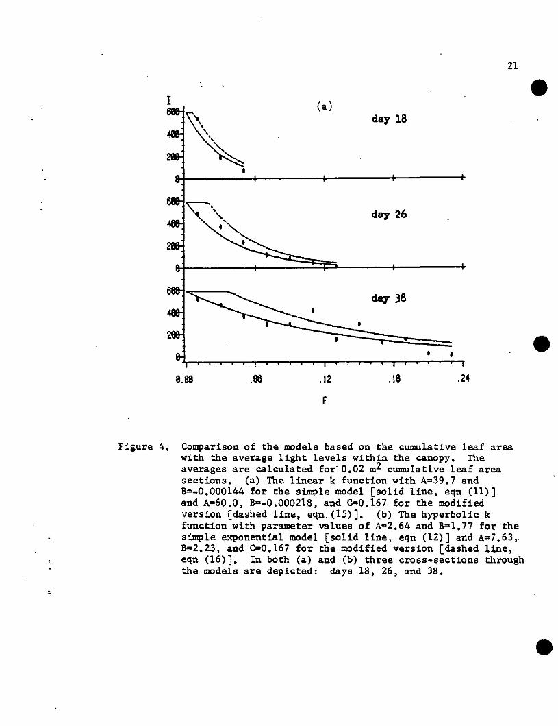
single day alone would represent a "best fit." Fig. 4 illustrates how
the models compare with the average light levels in the canopy at
several developmental stages. Model predictions based on cumulative
leaf area [eqns (11)-(12). (15)-(16») are compared to the average light
levels within levels of the canopy for days 18,,26. and 38 (Fig. 4).
For the particular dates. the simple exponential models with linear k
functions [Fig. 4(a») appear to fit slightly better for days 18 and 38
than the hyperbolic functions [Fig 4(b)]. and vice versa for day 26.
This may indicate that the linear models perform better for early and
late stages of canopy development. whereas the hyperbolic model does
better in the central section of the range. However. outside the
experimental range of the independent canopy variable the linear models
eventually predict negative values of k and. hence. exponentially
increasing models; the hyperbolic form approaches an asymptote and thus
may be better for extrapolation to larger canopies where this asymptote
is positive (i.e •• model l6H. Table 2) •
,
I...",
'." '-~
•
(a)daT 18
daT 26
21
•
daT 38
•• •• •
i i i
11.88 .96 .12 .18 .24
F
Figure 4. Comparison of the models based on the cumulative leaf areawith the average light levels within the canopy. Theaverages are calculated for' 0.02 m2 cumulative leaf areasections. (a) The linear k function with A=39.7 andB=-O.OOOl44 for the simple model [solid line, eqn (11)]and A=60.0, 8=-0.000218, and C=0.167 for the modifiedversion [dashed line, eqn. (15)]. (b) The hyperbolic kfunction with parameter values of A=2.64 and B=1.77 for thesimple exponential model [solid line, eqn (12)] and A=7.63,.8=2.23, and C=0.167 for the modified version [dashed line,eqn (16)]. In both (a) and (b) three cross-sections throughthe models are depicted: days 18, 26, and 38.
•

•
•
I
9.89 .96
'" ..
.12
F
•
day 18
day 26
day 38
.18
• •.24
22
•
Figure 4. continued

23
The effect of incorporating these light models within the
photosynthesis function of the snap bean growth simulation model was
evaluated by defining an arbitrary criterion index. It would be
desirable to minimize the predictive error for light intensity in that
portion of the canopy containing the greatest leaf surface area ,(generally the upper region of the canopy). 10 order to assess each
model with regard to its prediction error for these leaves, an index (y)
was de rived:
•
y = I:I,
(19)
where It and i.e are the observed and calculated irradiance values at
each leaf, I., and ~ is the leaf area of each leaf. It can be seen that
y takes on values between 0 (a perfect fit) and 1 (for a model which
predicts ~ to.within~ 10 ); however, the practical range of Y is much.
less than 1. For. any given data set, lower values for Y indicate better
performance of the simulator for larger leaves although no statistical
significanc~ can be attached. The Y values in Table 2 indicate that the
modified exponential with C-o.167 performed better for these leaves than
the corresponding simple and modified exponential models with all
parameters being fit. Those based on leaf area [eqns (15)-(16»)
performed better than those based on depth. It should be noted that the
best fit in this sense was not determined.
CONCLUSIONS
For snap bean, a simple exponential model provides a good
•
approximation to canopy light attenuation during canopy development.
Although the assumption of a continuous canopy during the early stages •

•
•
•
24
of development is clearly not met, the simultaneous least-squares fitted
models resulted in reasonable estimates during this period (e.g., day
18, Fig. 4). Based on the criterion-- index, Y, the modified exponential
models should provide the best estimate of canopy light attenuation for
computing canopy photosynthesis. It did not appear that the transition
from vegetative to reproductive growth (ca. days 25-28) affected the
performance of the light models, although this is a potential source of
prediction error.
There was no discernible difference in the use of canopy depth (X)
and leaf area (F) as independent variables in the light models.
However, for practical use in a simulation model, leaf area would be the
preferred variable. Leaf area has been the major variable used in field
studies of light interception, although this is not true for
controlled-environment studies where canopy studies such as reported in
this paper are rare (McCree, 1979).
Further applicability of these models might be achieved by
investigating how the parameters and variables considered here correlate
with measured variables of interest in the area of application. In air
pollution research, for instance, a change in the leaf transmission
coefficient (T) may be expected in stressed leaves. This would suggest
making k a function of the expected injury in addition to total leaf
area .

25
REFERENCES
Acock, B., Thornley, J.H.M., and Warren Wilson, J., 1970. Spatialvariation 'of light in the canopy. In: Prediction and Measurement ~of Photosynthetic Productivity, Proceedings of the IBP/PP TechnicalMeeting, Trebon, Czechoslovakia, Sept., 1969, ed. I. Setlik,pp. 91-102, PUDOC, Wageningen.
Council, K.A. and Helwig, J.T., eds., 1981. SAS/GRAPH User's Guide,1981 Edition. SAS Institute Inc., P.O. Box 8000, cary, NC 27511.
Downs, R.J. and Bonaminio, V.P., 1976. Phytotron Procedural Manual forControlled-Environment Research at the Southeastern PlantEnvironment Laboratories. North-carolina Agricultural ExperimentStation, Technical Bulletin No. 244, N.C. State University,Raleigh, NC.
Draper, N.R. and Smith, H., 1966. Applied Regression Analysis. Wileyand Sons, New York, 407 p.
Fuchs, M. and Stanhill, G., 1980. Row structure and foliage geometry asdeterminants of the interception of light rays in a sorghum rowcanopy. Plant, Cell and Environ. 3:175-182.
Helwig, J.T. and Council, K.A., 1979. The SAS User's Guide.Edition. SAS Institute, Inc., P.O. Box 10066, Raleigh,
1979NC. •Lemeur, .R. and Blad, B.L., 1974. A critical review of light models for
estimating the shortwave radiation regime of plant canopies.Agric. Heteorol. 14:255-286.
Loomis, R.S. and Williams, W.A., 1969. Productivity and the morphologyof crop stands: patterns with leaves. In: Physiological Aspectsof Crop Yield, eds. J. Eastin, F. Haskins, C. Sullivan, and C. vanBavel, Amer. Soc. Agron. and Crop Sci. Soc. Amer., Madison, WI,pp. 27-47.
Mann, J.E. and Curry, G.L., 1977. A sunfleck theory for general foliagelocation distributions. !. Math. Biology 5:87-97.
Mann, J.E., Curry, G.L., DeMichele, D.W., and Baker, D.H.,penetration in a row-crop with random plant spacing.72: 131-142.
1980. LightAgronomy:!..
McCree, K.J., 1979. Radiation. In: Controlled Environment Guidelinesfor Plant Research, eds. Tibbitts, T.W. and Kozlowski, T.T.,
'ACademic Press, New York, pp. 11-28.
Monsi, M. and Szeki. T., 1953. Ueber den Lichtfaktor in den Pflanzengesellschaften und seine Bedeutung fuer die Stoffproduktion. ~.J. Bot. 14:22-52.
Monteith, J.L., 1965. Light distribution and photosynthesis in field •crops. Ann. Bot. 29:17-37.

Monteith, J.L., 1973. Principles of Environmental Physics. EdwardArnold, London, 241 p.
• Ross, J., 1977.'R8diation conditions in the plant stand.Biophysikalische Analyse Pflanzlicher Systeme, ed. K.Gustav Fischer Verlag, Jena, pp. 115-119.
fu:Unger,
26
Stamper, J.H. and Allen, J.C., 1979.photosynthetic rate in a tree.
A model of the dailyAgric. Meteorol. 20:459-481.
•
•
Thornley, J.H.M., 1976. Mathematical Models in Plant Physiology.Academic Press, London, 318 p.

27
II
PLANT GROWTH ANALYSIS:
A METHOD FOR QUANTIFYING THE EFFECTS OF
EPISODIC AIR POLLUTION STRESS ON PLANT GROWTH
•
•
•

•
•
•
28
ABSTRACT
A technique is developed for the analysis of plant growth in
experiments where a one-time short-term stress (such as gaseous air
pollution exposure) is applied during the ontogeny of the plant. The
method is worked out in detail for the Richards growth function and
applied to growth data of snap bean (Phaseolus vulgaris) exposed to
ozone. This resulted in the value for the percent reduction in the
growth rate (74% for the 0.60 ppm 03 level) and an index for the
recovery rate. Results from different studies are comparable. The
technique may also be utilized with effects other than stresses and for
multi-episodic and chronic events.

29
INTRODUCTION
Plant growth analysis (Hunt, 1978) has been used extensively by•
plant scientists for the purpose of quantifying patterns of plant growth
and development. The traditional methods involve estimating growth
rates by computing slopes between subsequent data points in a time
series (Radford, 1967; Hunt, 1978). More recently, a functional
approach has been taken in which empirical functions are fitted to data
using nonlinear regression (Hunt and Parsons, 1977; Causton et al.,
1978; Hunt, 1979; Venus and Causton, 1979; Hunt and Evans, 1980);
analysis of growth rates is possible in this case by considering the
derivatives of the fitted function. A detailed comparison of the two
methods is given by Hunt (1979). •
Many different mathematical functions are available- for use in the
analysis of plant growth. These differ in complexity and in derivation.
Some, such as the logistic model, are based on observed patterns of
growth, whereas others, such as polynomial functions, are arbitrarily
selected for their ability to mimic data.
Two functions that have received a great deal of attention are the
logistic and Gompertz models. The former is the solution of the
differential equation:
dW • kW(l _ W)dt A
and the latter is the solution of:
(1)
dW • kW(ln A - In W)dt
(2)
•

•30
where Wis the plant attribute being studied and k and A are parameters.
In both equations, the right side represents the derivation based on the
observed growth pattern. When W is small, dW/dt is approximately
proportional to W; this represents an exponential growth phase. As W
approaches A, dW/dt approaches 0 asymptotically; this represents the
approach to a maximal size.
Richards (1959) reformulated the differential equations [eqns (1)
or (2)] to make the solution more general in its empirical
applicability. The differential equation is
•and its solution, generally called the Richards function (hereafter
abbreviated RF), is of the form:
W a A[l + sign(n)exp(C - kt)]-l/n
Again, A defines the upper asymptote of W, and n, C, and k are
(3)
(4)
•
parame~ers that determine the lower asymptote and shape of the growth
curve with respect to A. Note that when na 1, eqn (4) reduces to the
logistic model [eqn (1)] and as n~O, the Gompertz growth curve
[eqn (2)] is approximated (Richards, 1959). A comprehensive review and
guide to application of the RF is given by Causton et al. (1978) and a
review of growth functions in general can be found in Richards (1969).
Plant growth analysis has been successfully employed in studies of
the effects of various types of treatments on growth rates. In cases
where the functional approach has been taken, this has generally
consisted of fitting a characteristic growth function (e.g., logistic,
exponential, polynomials, etc.) to growth data from each treatment.

31
In experiments where a treatment commences sometime during the
development of the plant, this tyPe of analysis is not very effective
since a discontinuity in the growth rate, brought on by such an event,
cannot be Simulated using this method. It is, however, possible to
modify this analysis by allowing for such situations in the underlying
derivations of the growth functions.
In general, the growth of a plant or plant part can be written as a
differential equation of the form:
•
dW m feW)dt
where feW) is a function as in the right-hand sides of eqns (1)-(3).
(5)
One way to account for sudden changes in growth is to define a function
get) which is incorporated into eqn (5): •
~ m f(W)g(t)dt
where g(t)a1 for t prior to the time of the event (tevent), and
o i get) i 1 for t ~ tevent if the event is a stress (decreases
growth), or g(t) ~ 1 for t ~ tevent if the treatment increases the
(6)
growth rate. °If an eventual return to the growth pattern given by eqn
(5) is evident, then g(t) would again equal 1 after that time.
If application is made to the differential equation leading to the
RF [eqn (3)], eqn (6) can be written as follows:
:~ m ~ W [1 - (~)n]g(t)
the solution to eqn (7) is given by :
(7)
•

• J dW
W[l_(~tJ
32
(8)
The left side of eqn (8) is solved as for the RF:
AndW• Swn+l[(An;wn)_IJ
(9)
•
Setting u • (An/Wn) - 1, so that du • -nAn W-(n+l)dW,
eqn (9) can be rewritten as:
_.!.. J _nAn W-(n+l)dW • _ 1 r dun (Aniwa) _ 1 n J u
= - .!.. In Iu I + cn
• -.!.. In/(AnIWn ) - 11 + Cn
In all practical situations A > W so that (An/Wn)-l ~ 0 when
n ~ 0; this yields:
J_--=dW~_
W [1 - (~t](10)
With the right sides of eqns (8) and (10) being equal, we get:
In [(An;wn) - 1] = -k Sg(t)dt + C
The derivation for n < 0 is similar: let n=-m (m > 0), then in the same
way as eqn (10):
•=
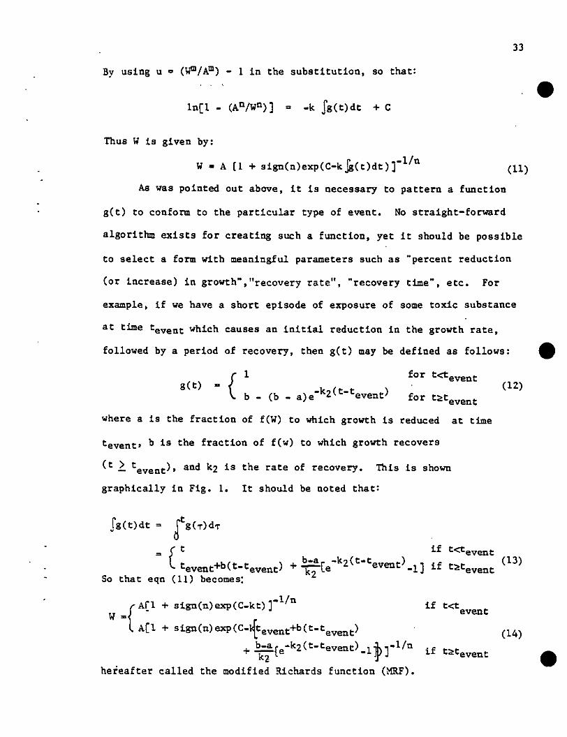
33
By using u 0 (wm/Am) - 1 in the substitution, so that:
•1n[1 - (An/Wn») = -k Sg(t)dt + C
Thus W is given by:
r_ )-l/nW • A [1 + sign(n)exp(C-kJS(t)dt)
As was pointed out above, it is necessary to pattern a function
get) to conform to the particular type of event. No straight-forward
(11)
algorithm exists for creating such a function, yet it should be possible
to select a form with meaningful parameters such as "percent reduction
(or increase) in growth","recovery rate", "recovery time", etc. For
example, if we have a short episode of exposure of some toxic substance
at time tevent which causes an initial reduction in the growth rate,
followed by a period of recovery, then get) may be defined as follows: •
get) o { 1b _ (b _ a)e-k2(t-tevent)
for t<tevent
for t~tevent
(12)
where a is the fraction of feW) to which growth is reduced at time
tevent' b is the fraction of few) to which growth recovers
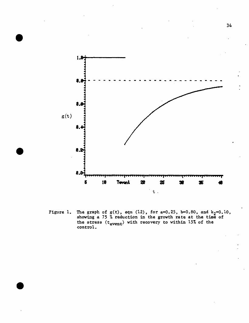
(t ~ tevent)' and k2 is the rate of recovery. This is shown
graphically in Fig. 1. It should be noted that:
Sg(t)dt = Jtg(T)dT
= [ :event+b(t-tevent)So that eqn (11) becomes:
fAC1 +
W=A[l +
sign(n)exp(C_kt»)_l/n
Sign(n)exp(C-{tevent+b(t-tevent)
+ .!!.=.{e-k2(t-tevent) _1 ;h)_l/nkZ f
hereafter called the modified Richards function (MRF).
if t<t teven
if t~tevent
(14)
•
•
•
get)
34
1.8+-----
- - - - - - - - - - - - - - - - - - - - - - - - - - -
8.
8.
8.,..,.............,..._....,............"""'............,................._'"""""'..........,.s 18
t
38 s
•
Figure 1. The graph of g(t), eqn (12), for a=0.25, b=0.80, and k2=0.10,showing a 75 % reduction in the growth rate at the time ofthe stress (tevent) with recovery to within 15% of thecontrol.

35
In the present paper, the RF and MRF are applied to growth data
from phytotron-grown snap bean (Phaseolus vulgaris L.) plants exposed to
various concentrations of ozone. The main objective is to contrast the
different methods of growth analysis implicit in these two equations
[eqns (4) and (l4)] through a quantitative assessment of the effects of
an episodic air pollution event on the growth rate of this species.
METHODS AND MATERIALS
•
Experimental Design
Snap bean plants (~ vulgaris L. cv. 'Bush Blue Lake 290') were
grown under controlled conditions in the Southeastern Plant Environment
Laboratory. Walk-in chambers used to house the plants during their •
ontogeny were limited in size so the experiment was carried out in two
phases, using identical conditions. Treatments consisted of exposing 15
day old plants to one 3 hour exposure of ozone at concentrations of
(experiment A) 0.00, 0.15, and 0.30 ppm, and (experiment B) 0.00, 0.45,
and 0.60 ppm administered in special exposure chambers (Heck et a1.,
1978) •
Seeds were placed in 250 ml styrofoam cups filled with standard
phytotron soil mixture (Downs and Bonaminio, 1976) at a density of 4
seeds per cup. After 8 days, the seedlings were repotted into 15.2 cm
diameter pots (same soil medium) at a density of 1 per pot, selecting
equally sized plants.
The same growth environment was maintained during the course of
both experiments: day lengths of 9 hours at 26· C and 15 hours •

•
•
•
36
(uninterrupted) nights at 22° C. Nutrient solution was applied each
morning, and deionized water in the afternoon in sufficient quantities
to drip through the pots. Irradiance during the day was kept constant
by maintaining a fixed proportion of incandescent and fluorescent lights
(Downs and Bonaminio, 1976) resulting in approximately 590 ~Em-2 s-l
at the top of the canopy.
Due to the small size of the ozone exposure chambers, plants were
exposed in two shifts: half in the morning, half in the afternoon.
Plants were watered approximately one hour prior to exposure. Once the
chamber microenvironment stabilized at a temperature of 26° C and
relative humidity of 70-80%, ozone generated with an electric .silent
discharge apparatus was introduced into the input air stream to obtain
the desired concentrations in the exposure chambers (monitored with a
Dasibi ozone analyzer).
After exposure, the plants were returned to the growth chambers,
where the pots were positioned so as to constitute homogeneous canopies
consisting of the same ozone treatment. A perimeter of pots containing
extra (non-control, non-treatment) plants was positioned around the
ensemble so as to reduce edge effects.
Plant harvests were carried out every three days from days 5 to 14
and every four days from days 18 to 38. Total dry weights (above and
below-ground parts) were determined after ovendrying the plant material
at 60-70° C for one week. Hence, a separate data set for each treatment
of each experiment was obtained and the RF and MRF fitted to each; note
that the same pre-exposure (d < 15) harvest data were used for each
treatment. The resulting parameter values were then analyzed for
trends.

••
•
•
37
In the present study the nonlinear least squares fitting of the RF
and MaF to these data were accomplished using the Statistical Analysis
System (Helwig and Council, 1979). Computer graphics were generated
directly from the results using SAS/GRAPH (Council and Helwig, 1981).
Fitting Strategies
To apply the MRF to data, it is necessary to have access to an
electronic computer equipped with an efficient nonlinear regress1.oa
algorithm. Even so, the experienced modeler will probably encounter a
great deal of difficulty since rarely are data available that are both
accurate and plentiful to warrant a seven parameter model. It is,
however, possible to reduce the problem so as to facilitate the fitting
and the interpretation of the results. In developing the MRF it was
implicitly assumed that eqn (5) would represent the control data and eqn
(6) the stressed plants; it is logical to also apply this assumption to
the data. This is accomplished by fitting the RF to the control data in
order to obtain estimates for A, k, C, and n of eqn (14) which leaves
only a, b, and k2 to be estimated. This procedure then allows
interpretations of the results in terms of the control curve.
Additional simplifications may be possible by restricting certain
model parameters. For example, if the growth rate recovery is assumed
to be complete, then b-l. If logistic growth is assumed, then n-l. In
situations where stress has a negative effect on the growth rate, then
bound a<l. The upper asymptote, A, may be bounded if its value (or
confidence interval) is known.
It 1s also recommended by Causton et al. (1978) that a logarithmic
transformation be made both to the data and to eqns (4) and (14) since

38
the error structure of growth data is usually a lognormal distribution.
If this is not done the nonlinear regression routines (which usually
assume a normal distribution for the error) may converge to the wrong
point or possibly not at all.
RESULTS AND DISCUSSION
•
The results of fitting the Richards function [RF, eqn(4)] to the
total dry weight data from experiments A and B are presented in the
upper portion of Table 1. The resulting curves, as well as the mean
. total dry weight at each harvest date, are shown in Fig. 2. These
models appear to provide reasonable descriptions of the data (see the
mean square error in Table 1). •
The results of fitting the modified Richards function, [MRF, eqn
(14)]. to the same data are presented in the lower portion of Table 1
and illustrated in Fig. 3. The four paramaters of the MaF that
represent the RF were fixed at those values estimated from the control
data as described above. Furthermore. it was assumed that the plant
growth rate would return to the rate of the control plants some time
after exposure (i.e •• 100% recovery) so that b [see eqn(12)] was set to
one; hence only two parameters. a and K2' needed to be determined by
the nonlinear regression routine. The mean square errors given in Table
1 indicate that these fits compare favorably to those of the RF. a fact
which can be seen by comparing Figs. 2 and 3.
The two methoda of growth analysis can be contrasted by (1)
comparing the resulting graphics (Figs. 2 and 3) and (2) noting the
types of patterns exhibited by the parameter values. With regard to the •

•
•
•
39
Table 1. Parameter values resulting from fitting the Richards function(RF) to the total dry weight data (top part) and from fitting themodified Richards function (MRF) utilizing parameter values in the03 = 0.00 columns for the other treatments in each experiment andfixing b = 1 (bottom part).
Ozone Treatments (ppm)Experiment A Experiment B
GrowthModel 0.00 0.15 0.30 0.00 0.45 0.60
Log A 2.747 2.714 2.880 2.441 2.287 3.027
C 0.9856 1.017 0.1789 3.402 2.797 -0.7920
k 0.07642 0.07776 0.06105 0.1441 0.1221 0.04884RF
n 0.2098· 0.2144 0.1246 0.6190 0.5401 0.06116
----- -------------- ---------------Mean
Square 0.03208 0.02882 0.03421 0.04041 0.05095 0.08060Error
a - 1.0000* 0.8472 - 0.6427 0.2613
k2 -- 0.0407+ 0.04133 - 0.07025 0.1000
MRF ----- -------------- - - - - - - - - - - - - - _.-Mean
Square -- 0.02668 0.03280 - 0.04943 0.06848Error
* iteration stopped at upper bound.
+ when a = 1.0, k2 is irrelevant .
40
19. , •7.S
9.
5.T0T 2.AL
9.DR I
Y\9.
UE 7. •IGH 5.T
2.5
9 \9 29
T
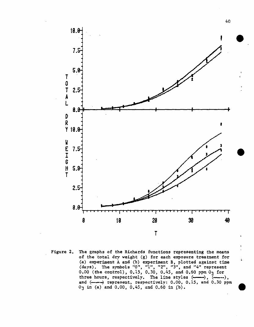
, Figure 2. The graphs of the Richards functions representing the meansof the 'total dry weight (g) for each exposure treatment for(a) experiment A and (b) experiment B, plotted against time(days). The symbols "0", "1", !t2", "3", and "4" represent0.00 (the control), 0.15, 0.30, 0.45, and 0.60 ppm 03 forthree hours, respectively. The line styles (-), (--),an~ (-----1 represent, respectively: 0.00, 0.15, and 0.30 ppm03 in (a) and 0.00, 0.45, and 0.60 in fb). •

,
8.
41
5.T0T 2.AL
8.0R •Y 18.
"• E 7.I6If 5.T
2.
•
8 18 28 38
T
•
Figure 3. The graphs of the Richards functions fitted to the controldata (solid line) for (a) experiment A and (b) experiment B.The symbols "0", "1", "2", "3", and "4" represent 0.00 (thecontrol), 0.15, 0.30, 0.45, and 0.60 ppm 03 for three hours,respectively. The line styles ~--_.) and (-__) represent,respectively: 0.15 and 0.30 ppm 03 in (a) and 0.45 and 0.60in (b) •

42
former, the MRF provides a more realistic description since it correctly
predicts the pre-exposure growth pattern [note that the RF predicts ~
different total dry weights for plants treated in the same way between
days 11 and 15; see Fig. 2(b)] and simulates the ozone exposure event
(see kink in curves st day 15 in Fig. 3).
Trends in the parameter values across the various ozone treatments
are of significance since such patterns may suggest possible
interpolation for effects of doses other than those used in the
experimentation. Of course, in cases where no trend is evident, this
practice cannot be justified. Where parameter trends can be identified,
their pattern may be modeled using empirical mathematical functions and,
subsequently, used for making predictions. It can be seen in Fig. 4
that the fitted parameters a and k2 of the MRF show distinct patterns
across the ozone treatments; on the other hand, this is not the case for
the 4 fitted parameters of the RF (see Fig. 5).
•Furthermore, the MRF is superior in that it provides new insight
into the effect of ozone exposure on snap bean by quantifying the degree
to which growth is affected. It can be seen that the growth rate
immediately following exposure is reduced from 100% at 0.15 ppm to 26%
at 0.60 ppm as measured by the parameter a (see Table 1 and Fig. 5).
The parameter k2' which serves as an indicator of the recovery of the
growth rate shows an increasing trend with ozone concentration, although
more data for other ozone levels need to be obtained before any
conclusive statements regarding this can be made.
In order to further examine possible applications of eqn (6), an
extension was made for multiple episodic events. This calls for
extending eqn (6) to obtain the differential equation: •

431.8 (a)•• 8.8
8.6a
8.4
8.2
8.8
8.' 8.68
(b)
8.
k2 8.
8.
8.
8.68 8.1S 8.J
•
Ozone Concentration (ppm)
Figure 4. The parameter values of a and k2 of eqn (14) plotted againstozone dose. Note the smooth patterns •
•

44
3. •3. a a
LogA 2. Da
2.I.3. a2.
c I. a8. a
..I.
.I a
.Iak • a •a
8.8. a
n 8.8. D a D
8.88 8.15 e.! 8A5 8.1
Oz~ con.c.cntration (ppm)
Figure 5. The parameter values of LogA, C, k, and n of eqn (4) plottedagainst ozone dose. Note the lack of trends.
•

• dW- ..dt
(15)
45
where each gi(t) represents the modification in the growth rate due to
the ith event. The solution of eqn (15)
- -linA[I-+ sign(n)exp(C-kt)]
W D
is given by:
for tS min{t t }i even i
(16)
ij -lIn {}A[l + sign(n)exp(C-k IT 8i (t)dt)] for t> min tevent
i .. l i iIn order to apply eqn (16) to multiple episodic ozone exposures,
experiment A was repeated for the 0.30 ppm treatment with
the exposure days, of 15, 18, 21, 24, and 27. A computer
teventi •program was
evaluate the integral. Since the same stress was applied each time, the
written to evaluate eqn (16) numerically, using the trapezoidal rule to
be equal for
(17)
t < t eventi
for
for
same formulation of g was used:
gi (t) =11
-bi - (bi -ai )exp(-k2 (t-tevent »
i iThe values for ai and k2i were assumed to
•since insufficient data were available to allow each to vary
independently. Again, eqn (4) was fit to the control data (symbol ·0·,
Fig. 6) to obtain A, k, C, and n values [curve (1) in Fig. 6];
furthermore, values of a and k2 estimated for the 0.30 ppm treatment
described earlier (0.8472 and 0.04133, respectively; Table 1) were used.
The resulting simulation overestimated mean total dry weight values
(symbol ·2·, Fig. 6) for all harvests after day 21 [curve- (2), Fig. 6].
This indicates that ai probably declines either with age at exposure
•(teventi) or the exposure number (i), suggesting a lower average
value for parameter a. In fact, rerunning the simulation with parameter

46
18.
••(1)
T 7.0T
"L0 (2)
R Ii.Y
" (3)EI •(;
H 2.T
8.
8 18 28
T
Figure 6. The Richards function [line (1») fitted to control total dryweight data from the multiple episodic experiment (see text).The symbols "0" and "Z" represent the means of the harvestsof the control and 0.30 ppm 03 five times for three hours,respectively. Line (2) represents eqn (16) with a=0.85 andkZ=0.413; line (3) represents eqn (16) with a=0.75 andk2=0.05. (b=l in both evaluations).
•
-.
•
•
47
a reduced 13% and k2 increased 21% (i.e., a • 0.75 and k2 • 0.05),
yielded a much better fit to the data [see curve (3), Fig. 6).
SUMMARY
1. The modified Richards function, as given by eqn (14), was applied to
growth data from phytotron-grown snap bean plants subjected to epis~dic
ozone exposures. By selecting a formulation of g(t) which corresponded
to hypothesized effects, results were obtained which provide a
quantitative assessment of the changes in the growth rate, pe.rm1tting
prediction of responses to treatments of other ozone concentrations.
2. The initial grOwth rate reduction of snap bean plants exposed to
various levels of ozone concentration for 3 hours was found to increase
from 15% at 0.30 ppm to 74% at 0.60 ppm.
3. The modified Richards function provides a valuable tool for analyses
of treatments affecting plant growth in which a control curve can be
simulated using the Richards function. Applications range from
detrimental to beneficial effects and from single-event short-term to
long-term chronic events. Various causes, such as herbicides, water
deficiency, insect infestations, pollutants, or temperature
fluctuations, may be analyzed, although different formulations of g(t)
may be necessary. These should be limited to functions containing
parameters which have meaning. Otherwise, there is no advantage over
the traditional functional approach •

48
REFERENCES
Causton, D.R., Elias, C.O., and Hadley, P., 1978. Biometrical studiesof plant growth. I. The Richards function and its applicationsin analyzing the effects of temperature on leaf growth. Pl. Cell.Environ. 1, 163-84.
Council, K.A., and HelWig, J.T., eds., 1981. SAS/GRAPH User's Guide,l2!! Edition. SAS Institute, Inc., P.O. Box 8000, Cary, Nc 27511.
Downs, R.J. and Bonaminio, V.P., 1976. Phytotron Procedural Manual~Controlled-Environment Research at the Southeastern PlantEnvironment Laboratories. North-carorina Agricultural ExperimentStation, TechnIcal Bulletin No. 244, NC State University, Raleigh,NC 27650.
Heck, W.W., Philbeck, R.B., and Dunning, J.A., 1978. A continuousstirred tank reactor (CSTR) system for exposing plants to gaseousair contaminants. Principles, specifications, construction, andoperation. Agricultural Research Service, U.S. Department ofAgriculture, ARS-S-18l, 32 pp.
Helwig, J.T. and Council, K.A., 1979. The SAS User's Guide. 1979Edition. SAS Institute, Inc. P.0:-Box-l0066, Raleigh, NC-:Z7650.
Hunt, R., 1978. Plant Growth Analysis. Edward Arnold, London. pp. 67.
•
•Hunt, R., 1979. Plant growth analysis:
the fitted mathematical function.The rationale behind the use of~~ 43, 245-249.
Hunt, R. and Evans, G.C., 1980. Classical data on the growth of maize:curve fitting With statistical analysis. ~ Phytol. 86, 155-180.
Hunt, R. and Parsons, ~.T., 1977. Plant growth analysis: furtherapplications of a recent curve-fitting program. ~ Appl. Rcol. 15,965-968.
Radford, P.J., 1967. Growth analysis formulae - their use and abuse.crop~, 7, 171-175.
Richards, F.J., 1959. A flexible growth function for experimental use.~ Exper. ~, 10, 290-300.
Richards, F.J., 1969. The quantitative analysis of growth.Physiology: A Treatise, ed.: F.C. Steward, pp. 3-76.Press, London7
In: PlantAcademic
Venus, J.C. and Causton, D.R., 1979. Plant growth analysis: The use ofthe Richards function as an alternative to polynomial exponentials.~~, 43, 623-632.
•

~
50
ABSTRAcr
A carbon-allocation model for the growth of a snap bean crop is
derived. Leaf photosynthesis is predicted using a nonrectangular
hyperbolic light response curve. The leaf area distribution in the
canopy is simulated and. thus. allows utilization of a simple light
interception model. This scheme allows integration over the canopy to
obtain the total daily production. Whole-plant respiration is estimated
using values obtained from the literature. Assimilate distribution is
modeled with an empirical formulation based on the ratio of: "plant
part (organ) dry matter increment" to "total dry weight increment." The
model can be adapted for use in studies involving effects on the leaf
compartment of the plant. in particular of gaseous pollutants which show
visible injury to the leaves. ~
~

-.
•
•
51
INTRODUCTION
In recent years much effort and resources have been invested in an
attempt to understand the physiology of whole plants. ~ithin this body
of science much work has -been done on separate subsystems of the whole
organism in order to understand the function of each by itself, in the
hope that, when all subsystems are put together into one descriptive
paradigm, the whole organism will be understood. This combining process
is the basis for modeling. In general, however, models cannot achieve
this complete description because of their inability to mechanistically
describe each detail of the whole organism. It is always necessary to
reduce the framework of the model so that only a subset of the subject
is modeled (Thesen, 1974). The resulting models, although usually
falling short of this goal, are generally valuable tools for studying
effects of induced environmental changes on the growth dynamics of the
plants.
Thus every modeler is faced with the task of first conceiving what
Zeigler (1976) calls "the base model" (the unattainable hypothetical
complete explanation) and then formulating "the lumped model" (the
simplification) by retaining only those elements of the base model which
coincide with the objectives of the project. For example, in the
present study a model is being developed to be used as a tool for
studying the effects of gaseous pollutants on agricultural plants.
Hence, the model has to deal explicitly with the foliage, since this is
the primary site of damage (Heck and Tingey, 1970; Craker and Starbuck,
1972; Evans and Ting, 1974; Manning and Feder, 1976), and should also
include the photosynthetic process since it has been shown to be

52
affected (Todd~ 1958; Hill and Bennett, 1970; Bennett and Hill, 1973;
Pell and Brennan, 1973; Capron and Mansfield, 1976; Heath, 1980). Yet,
care should be taken as to how detailed a photosynthesis model to use.
If intricate biochemical theories are to 'be tested, models such as those
of Farquhar et al. (1980) or Hall (1979) should be considered. In the
present paper such complexity was unnecessary and intractible; a simple
response function [see Thornley (1976) for review] was found to
suffice.
The model developed here is designed for simulating the growth of
snap bean (Phaseolus vulgaris L. cv. 'Bush Blue Lake 290') in
controlled-environment conditions, although extension to other species
and varying conditions are possible. The objective is to develop a
model which will be suitable for testing theories concerning the effect
of the gaseous pollutant ozone on plant growth and development.
MODEL STRUCTURE
In virtually all simulation models, the fate of one or two forms of
energy or mass are traced subject to the laws of conservation of mass
and energy. In its Simplest form, this calls for using one entity
(e.g., carbon, water, or nitrogen). In the present paper a carbon-flow
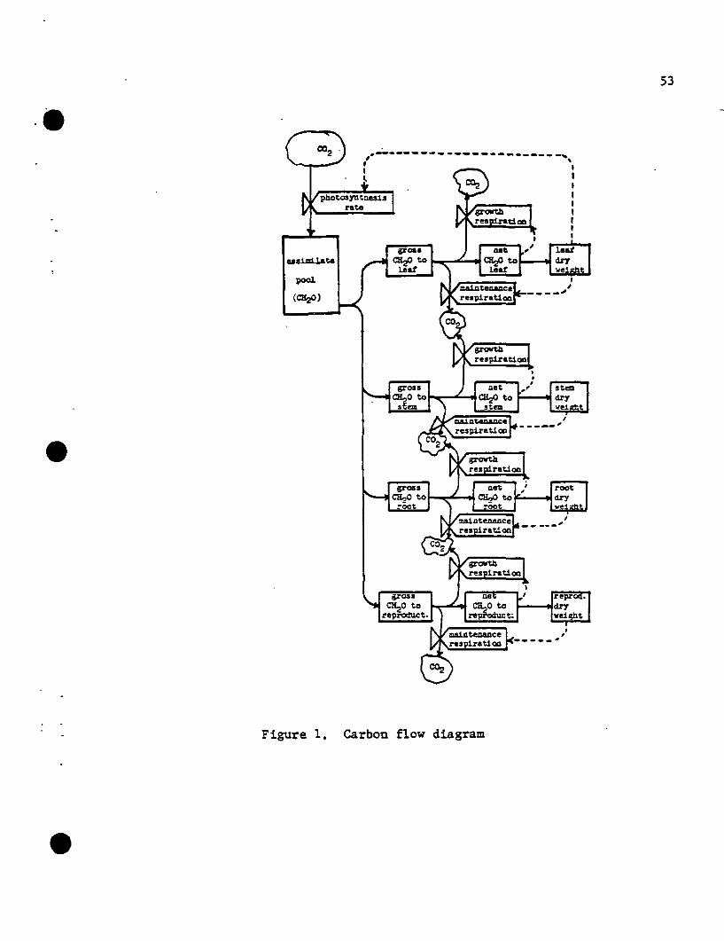
model was developed (see Fig. 1). Carbon (glucose) enters the system
through the photo~ynthetic process and is distributed over four compart
ments (Leaf, Stem, Root, and Reproductive). In the conversion of this
carbon substrate to plant material (measured in grams dry weight) a
portion is respired. A feedback in the loop occurs through the leaf
•
•
compartment, whose size and leaf distribution affect the amount of •
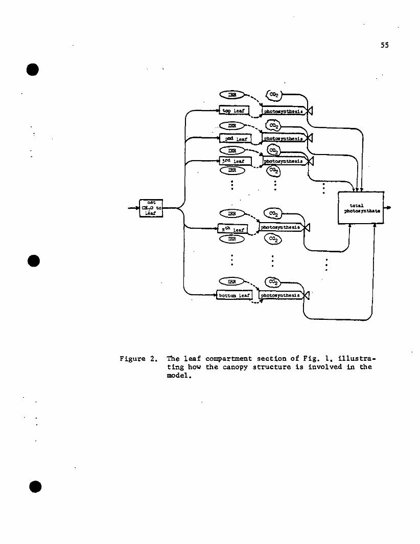
photosynthate produced. The model includes the effects of canopy archi
tecture (i.e.; leaf area distribution, light distribution) and the leaf
u.1m1l&te
53
,----- --- --------------..., ,I I
l IIII,III
pocl
(C¥J
•
•
Figure 1, carbon flow diagram
•

age distribution on productivity (see Fig. 2). Leaf location infor
mation is retained and the vertical leaf area distribution calculated.
54
•Using a light interception model, it is possible to calculate the avail-
able photosynthetically 'active radiation (PhAR) directly above any leaf
(symbol IRR in Fig. 2). Thus a response function based on leaf area,
light availability and age of tissue is used to predict photosynthesis.
Photosynthate in the leaf compartment is partitioned among the
individual leaves through a scheme based on "sink strengths." Since
rapidly growing leaves require more substrate than mature leaves, a leaf
allocation scheme can be worked out based on the leaf expansion curve.
With the proper conversion coefficient (m2 leaf area per g CH20
allocated), the canopy structure can be defined.
The time frame of the model is on the order of 5-10 weeks with
increments of· 1 day. TWo time variables are used: d, the number of
days after sowing, and t, leaf age (where tt is the age, in days, of
leaf ~).
Irradiance
Many light interception models are available from the literature
ranging from simple exponential decay models (Monsi and Saeki, 1953;
Monteith, 1965) to complex formulations which rely on factors important
to specific types of systems, e.g., sunflecking (Mann and Curry. 1977),
phytomatter distribution (e.g.: Acock et al., 1970; Meyer et al.,
1979; Lieth, 1982), and leaf angles (e.g., Loomis and Williams, 1969).
The formulation of Lieth (1982) is used here because of its simplicity.
Due to the elaborate structure whereby the canopy architecture is
•
defined in this study, it is possible to use an attenuation model based •
on cumulative leaf area to predict PhAR at each leaf. The form selected
•
•
•
55
C§>....., ~I""" leat I I tl1ed, (1
.- G}cg:r--. CO:!
2"'1 leat I I "1:1otolI1md1eds a~..::~~,rd lear I tl1ed, r! ......
~ ...~ .• • •• • ,\,• • •·
oat I
C§>...• ®total f--ClL,O to
_yntll&tsliat ~,
.th 1.... I Ipbotosynth.d, 1{1
C§::) .' @i>
• •· • •• • •·~"" <3>botteD. leat I Ipbo~1a:thes1s kl..... ...
Figure 2. The leaf compartment section of Fig. 1. illustrating how the canopy structure is involved in themodel •

56
here is:
for F < CFtot
for F ~ CFtot(1) •
where I is the PhAR, Io the value of I at the top of the canopy, F the
cumulative leaf area above a leaf, Ftot the total leaf area of the
plant, C the fraction of the total leaf area in the top of the canopy
which is exposed to full light (Io) and k the extinction coefficient.
The latter was found to vary with Ftot as follows:
k = A + B/Ftot
where A and B are empirical parameters.
Leaf Photosynthesis
(2)
A photosynthesis model employing irradiance and leaf age as the •
sole independent variables is quite reasonable within the framework of
the current research project (constant temperature and C02
concentration). Two commonly favored versions are the rectangular
hyperbola:
aI + Pg,max
and the nonrectangular hyperbola:
o = pie - Pg(aI + Pg,max) + aIPg,max
(3)
(4)
because of their origin in enzyme-substrate .kinetics (Rabinowitch, 1951;
Thornley, 1976, pp. 101-103). In both, Pg is the gross photosynthesis
rate, I is PhAR, a is the initial slope, Pg,max is the upper
asymptote and 8 is a dimensionless parameter with different meanings
depending upon the authors (see e.g., Prioul and Chartier, 1977;
Marshall and Biscoe, 1980).•

•
•
57
Eqn (3) is .the. form most commonly used by researchers studying bean
species (e.g., Tenhunen et al., 1976 a aud b; Meyer et al., 1979).
However, a major problem with its application to Phaseolus vulgaris has
been noted by several authors (see Marshall and Biscoe (1980) for
review). The difficulty is seen from the following example: Suppose
fran iuspection of CO2 exchange data, Pg ,max is estimated to range
-1from 400 to 1700 Ilg C02 m-2 s-l and a. from 1. 5 to 4.0 Ilg C02 IlEinstein
with values of 1000 for Pg,max and 2.0 for a. for a particular
observation in which saturation is attained for irradiance values well
below 2000 IJE m-2 s-l. Under these conditions, eqn (3) predicts 800
Ilg C02 m-2s-1, a 20% error.
In fact, the rectangular hyperbola couaistently underestimates the
photosynthetic rate if a. is estimated from the initial slope and
Pg,max from the maximal values in the data. On the other hand, if a.
and Pg,max are estimated by fitting eqn (3) to data using a nonlinear
regression routine, then t~ese would not accurately reflect the
physiological quantities which they are supposed to represent. This
inflexibility may be inherent in any model containing only the two
parameters and Pg,max'
Eqn (4) represents a family of curves whose explicit form for Pg
is:
•
O'I + Pg,max - ,haI + Pg,max) 2 - 4aIPg ,max9
26
with an applicable range for e of 0 to 1. In fact, if e D 0, eqn (4)
becomes algebraically equivalent to eqn (3) and if e a 1, the Blackman
limiting response curve results:
(5)
{
O'I. Pg ..
Pg,max
for I < Pg,max/a
for I ~ Pg,max/O'
58
(6) •To obtain a formulation for the net photosynthetic rate (Pn) one
simply applies the fact that:
Pn .. P - It L (7)g
where RL is the leaf respiration rate. In this model RL is assumed
to be constant over irradiance, so that we can also write:
Pn,max .. Pg,max - RL
As a result eqn (5) becomes:
(8)
•(9)
Q'I + Pn max + RL,P ..n
- '/ (aI+Pn max"ffiL) 2 - 4aI8(Pn max"ffiL), '- RL
28
In their work on Phaseolus vulgaris, Catsky and Ticha (1980) found
that a, Pn.max, and RL vary With the age (t) of the leaf tissue.
This suggests that the model parameters need to be computed as functions
of time:
a" aCt); Pn,max - Pn.max(t);
It should be noted that eqn (9) provides
(10)
a simulation for the net
photosynthetic rate on a "per second" basis. This is done to facilitate
application of the model to situations where light will vary throughout
the day. In controlled-environment studies, where light is constant,
Pn needs only to be multiplied by the photoperiod (in seconds) in
order to obta~n the daily rate.
Respiration of each plant organ is evaluated in a separate submodel
so that the gross, rather than net photosynthesis rate has to be the
dependent variable of this submodel. Yet:
O'I + Pn max + RL -P ,g ..
'/ (a I+Pn,max+RL) 2 - 4aI8(Pn •max+RL)
28(11) •

•
•
59
is preferred rather than eqn (5) since available data are usually for
Pn, allowing the parameters of eqn (11) to be estimated directly.
To determine the total amount of gross photosynthate (W) produced
by the entire plant, the gross photosynthetic rate of each leaf
(Pg,t(t)) must be multiplied by its leaf area (At(d)) and this
product summed over all leaves:
Wed) = ! Pg,t(t)At(d) (12)
For Phaseolus vulgaris, the photosynthetic contribution of other organs
such as stem and pods to the photosynthetic pool is generally small
(Wallace et al., 1976) and can thus be ignored.
Respiration
Two components of respiration can be identified: maintenance and
growth respiration. Maintenance respiration, the total amount of carbon
utilized for the maintenance functions of the plant, has been shown to
be roughly proportional to the total dry weight of the plant and is
temperature dependent (McCree, 1970). Of the remaining assimilate, a
certain fraction, called growth respiration, is respired in the
synthesis of structural and storage compounds; this is directly related
to the gross photosynthetic rate and the compounds being synthesized but
independent of environmental conditions (Penning de Vries, 1972 and
1975).
Thus, if R is the total amount of carbon respired on a given day,
then:
where Wis daily gross photosynthesis, X represents the dry weight
compartments with subscripts defining which (L • leaf, S • stem, R =•R· kl[W + b (XL + Xs + XR + XF)] (13)

60
root, F a reproductive tissue), and kl and b are constants of
proportionality. It should be noted that eqn (13) is equivalent to the ~
one derived by McCree (1970) With kl' P, c, and Wof his paper
corresponding to k1, W, -klb, E Xi above.i
Using eqn (13) in the model results in a "net assimilate pool on day d
of:
(14)
Allocation
The net assimilate, Wn(d), is distributed according to the
requirements of the various plant parts (Wearing and Patrick, 1975).
Within the model, this can be done by defining partition coefficients,
Tt1 which represent the fraction of Wn(d) allocated to the plant part
(indicatd by the subscript) (e.g.: Monsi and Murata, 1970;
Charles-Edwards and Fisher, 1980) and computing the daily dry matter
increment,6Xr}d), by:...J
6Xejd) a ~(d) (15)
For reviews see Thornley (1976) and Hesketh and Jones (1980). Wilkerson
et al., (1981) allowed variations in the coefficients with the
physiological stages associated with reproduction. The same treatment
is necessary here since the shift from vegetative to reproductive growth
occurs quite early in the life cycle of the plant and will fall within
the time frame of the model. Thus we have:
~
b = TICd)
and the dry matter on day d+l of compartment 0 is given by:
(16)
(17)
•
.•
•
•
61
Canopy Characteristics
As seen in Fig. 1 two aspects of the canopy are dealt with in the'
computer simulation model: 1) canopy architecture and 2) allocation of
assimilates to individual leaves.
a. Canopy architecture
Whenever a leaf photosynthesis model is used within a crop model,
it is necessary to describe the architecture of the canopy so that
integration over the whole canopy will be possible. Within the
framework of this model, age, size, and location of each individual leaf
is important. Here, no specific statistical distribution was assumed,
but rather ~ a matrix containing two columns: one for the day of
initiation of any particular leaf and the other for its final location
within the canopy. The day of initiation is, for practical purposes,
the day on which the leaf begins to unfold. The canopy location is the
sequence number, from the top, for a mature canopy. It should be noted
that this ignores the process of leaves starting out near the main stem
of the plant and progressively mOVing outward and upward in the canopy
as the petiole elongates.
The matrix fwill have as many rows as there are leaves on the
typical plant. For this purpose a group of plants will have to be
surveyed and the structure of a "typical" plant identified.
b. Allocation of aSSimilates to individual leaves
As the individual leaf subcompartments grow, various canopy
characteristics are altered, affecting light availability and therefore
photosynthetic rates throughout the canopy. In order to simulate this
dynamic leaf area distribution, it is assumed that each leaf grows in a
genetically preprogrammed fashion, so that a leaf represents a strong
62
sink at times of rapid growth and a weak sink at times of low assimilate
utilization. If it is assumed that the growth pattern of the individual~
leaf is logistic over time, and is the same for all leaves, then we can
simulate sink strengths with one scheme for all plants. Thus Sl t),
the· strength due to the sink represented by leaf 1. (at time t) is given
by:
(18)
where q is a constant of proportionality and B, M, and k2 are
parameters of the logistic leaf growth curve. This function is used to
determine the fate of the available assimilate by diViding it up in
proportion to the sink strengths. Thus only the normalized values are
needed to designate what fraction each leaf gets. Thus it is convenient ...
to redefine S1.(t):
(19)
This scheme then determines the amount of assimilate apportioned to
each leaf. In cases where leaf dry weight is proportional to leaf area,
we can use AXL(d) to determine the increment in the leaf area for each
leaf:
DA1.(d) = p/lX1.(d)S1.(t) (20)
where p is the conversion factor for dry weight to area. This results
in leaf areas:
(21)
...

-•
•
•
63
DISCUSSION
In order to apply the model to a particular plant system, all
parameters and initial values of the model [eqns (1), (2), (10), (11),
(12), (14)-(17), and (20)-(22)] need to be known or approximated. In
some cases, parameters need to be replaced with functions [eqns (10) and
(15)]. Ideally these should be obtained from experiments designed for
this purpose on the plant cultivar to which_the model is to be tailored.
This will require a stand of plants grown under controlled conditions
with harvests at regular intervals. The canopy structure (n should be
determined by measuring leaf areas, light levels, and leaf locations, as
well as keeping track of leaf ages through a system which allows
identification of individual leaves. This information can also be used
to obtain the parameters 10 and C [eqn (1)], A and B [eqn (2)], and M,
B, and k2 [eqn (20)]. Photosynthetic rates would have to be measured
at various light levels (including saturation) for various leaf ages in
order to estimate the parameters of eqns (10) and (11). Harvests would
consist of separating plants into the various parts for dry weight
measurements so as to obtain the partitioning functions, eqn (15).
In order to get the dynamic model started, several initial values
will have to be obtained (for variables XL, XS, XR, and XF)' To
get these. it is important to first determine the time span over which
the simulation is to be carried out. The starting day determines the
day of the experiment on which the measurement needs to be made. In
most cases, experiments are started during the vegetative phase of the
plants, so that XF' the reproductive dry weight, is zero. In
situations where the starting day is soon after germination, it is
necessary to include an additional dry weight variable, XC' for the

64
seed cotyledons si~ce this is the only source of energy due to the fact
that the unfolding leaves of the seedling are too small and respire too
rapidly to generste enough energy to account for the rapid development
at that time.
The methods used to estimate the parameters and initial values
require certain assumptions. Some of these are "hidden" and care must
•
be taken in applying the model so that these are not violated. The main
underlying assumption is that the controlled conditions under which the
experiment was run are. in fact. controlled. When it is known that such
assumptions are violated. it has to be assumed that these have little or
no effect. If this assumption cannot be made. then it will have to
treated in the model. or the data cannot be used. Many
exist and the modeller should be aware of them so as to
such assumptions
avoid ~disasterous results. Furthermore. care should be taken to make sure
that there are no unreasonable assumptions.
Additional violations of assumptions may come about when those
environmental conditions under which the data is collected are not
controlled in the way the researcher thinks. This may be due to
mechanical failures (such as worn thermostats, solenoids. and other
technical equipment which maintain slightly different or possibly
varying conditions in the growth chamber). Ignorance may also result in
problems; the inexperienced research~r may, for example, not be aware of
the fact that light sources become gradually dimmer With age, resulting
in different incident PhAR levels towards the end of experiments lasting
several months.
Several modeling assumptions were also made in developing the •
model. The submodel used for light attenuation. for instance, assumes

••
•
•
65
that the canopy has an approximately homogeneous leaf distribution
(Lieth, 1982). In eqns (5), (9), and (11), the leaf respiration rate
RL is assumed to be constant over I, as is 6. The respiration
submodel, eqn (13), through its empirical development (McCree, 1970)
contains many assumptions; here we merely assume that it will adequately
approximate the actual situation. In the development of the allocation
submodel [eqn (15)) it was assumed that the dry weight increments of the
plant parts between harvests are proportional to the amount of
assimilates allocated. In setting up a fixed canopy architecture it is
assumed that such an average, as represented by r, will adequately and
reasonably correctly describe the plant.
It is felt that all these assumptions are reasonable and that the
model, in its present form, provides the necessary flexibility to be
utilized in various different types of studies of plant growth. In
particular, its design lends itself to analyses of effects of stimuli
which affect the leaves and the canopy architecture such as gaseous
pollutants•

66
REFERENCES •Acock, B., Thornley, J.H.M., and Warrenvariation of light in the canopy.of Photosynthetic Production, ed.:Viageningen, The Netherlands.
Wilson, J., 1970. SpatialIn: Prediction and MeasurementI. Setlick, pp.-g[-102, PUDOC,
Bennett, J.H. and Hill, A.C., 1973. Inhibition of apparentphotosynthesis by air pollutants. ~ Environ. Quality 2, 526-530.
Capron, T.M. and Mansfield, T.A., 1976. Inhibition of netphotosynthesis in tomatoe in air polluted With NO and N02' J.Exper. Bot. 27, 1181-1186.
- - I
Catsky, J. and Ticha, I., 1980. Ontogenetic changes in the internallimitations to bean-leaf photosynthesis. 5. Photosynthetic andphotorespiration rates and conductances for C02 transfer asaffected by irradiance. Photosynthetica 14, 392-400.
Charles-Edwards, D.A. and Fisher, M.J., 1980. A physiological approachto the analysis of crop growth data. I. Theoretical condiderations'~~ 46, 413-423.
Craker, L.E. and Starbuck, J.S., 1972.With ozone injury of bean leaves.
Metabolic changes associated~:!:. Plant~ 52, 589-597. •
Evans, L.S. and Ting, I.P., 1974. Ozone sensitivity of leaves:relationship to leaf water content, gas transfer resistance, andanatomical characteristics. Amer.:!:.~ 61, 592-597.
Farquhar, G.D., von Caemmerer, S" and Berry, J.A., 1980. A biochemicalmodel of photosynthetic C02 assimilation in leaves of C3species. Planta 149, 78-90.
Hall, A.E., 1979. A model of leaf photosynthesis and respiration forpredicting C02 assimilation in different environments. Oecologia(Berl.) 143, 299-316.
Heath, R.L., 1980. Initial events in injury to plants by airpollutants. ~~ Plant Phys. 31, 395-431.
Heck, W.W. and Tingey, D.T., 1971. Ozone. Time-concentration model topredict acute foliar injury. In: Proceedings of the SecondInternational Clean Air Congress, eds.: H.M. Englund and W.T.Beery, pp. 249-255. '"ACademic Press, NY.
Hesketh, J.D. and Jones, J.W., 1980. Integrating.traditional growthanalysis techniques With recent modeling of carbon and nitrogenmetabloism. In: Predicting Photosynthesis for Ecosystem Models,eds.: J.D. Hesketh and J.W. Jones, Vol. I, -pp. 51-92, CRC Press, •Inc., Boca Raton, Florida.

•
•
•
67
Hill, C.A. and.Bennett, J.H., 1970. Inhibition of apparentphotosynthesis by nitrogen oxides. Atmas. Envir. 4, 341-348.
Lieth, J.H., 1982. Light interception by a developing snap bean canopy.Ph.D. thesis, North Carolina State University, Raleigh, NC.
Loomis, R.S. and Williams, W.A., 1969. Productivity and the morphologyof crop stands: patterns with leaves. In: Physiological Aspectsof CHoP Yield, eds.: J. Eastin, F. Haskins, C. Sullivan, and C.Van avel, pp. 27-47. Amer. Soc. Agron. and Crop Sci. Soc. Amer.,Madison, NY.
McCree, K.J., 1970. An equation for the rate of respiration of whiteclover grown under controlled conditions. In: Prediction andMeasurement of Photosynthetic Productivity, ed. I. Setlik, PP7221-229, p~, Wageningen, The Netherlands.
Mann, J.E. and Curry, G.L., 1977. A sunfleck theory for general foliagelocation distribution. J. Math. BioI. 5, 87-97.
Manning, W.J. and Feder, W.A., 1976. Effects of ozone on economicplants. In: Effects of Air Pollutants on Plants, ed.: T.A.Mansfield, pp. 47-60,-cambridge University Press, Cambridge, UK •
Marshall, B. and Biscoe, P'V" 1980. A model for C3 leaves describingthe dependence of net photosynthesis on irradiance. I.Derivation. ~ Exp.~ 31, 29-39.
Meyer, G.B., Curry, R.B., Streeter, J.G., and Mederski, H.J., 1979.SOYMOD!OARDC - A dynamic simulator of soybean growth, developmentand seed yield: I. Theory, structure and validation. ResearchBulletin 1113, Ohio Agricultural Research and Development Center,Wooster, Ohio.
Monsi, M. and Murata, Y., 1970. Development of photosynthetic systemsas influenced by distribution of matter. In: Prediction andMeasurement of Photosynthetic Production, ed.: t. Setlik,-PP.115-129, PUDOC, Wageningen, The Netherlands.
Monsi, M. and Saeki, T., 1953. Ueber den Lichtfaktor in den Pflanzengesellschaften und seine Bedeutung fuer die Stoffproduktion. Jap.~~ 14, 22-52.
Monteith, J.L., 1965. Light distribution and photosynthesis in fieldcrops. ~~ 29, 17-37.
Pell, E.J. and Brennan, E., 1973. Changes in respiration,photosynthesis, ATP, and total aleny1ate content of ozonated pintobean foliage as they relate to symptom expression. Plant Physiol.51, 378-381 •

Penning de Vries, F.W.T., 1972. Respiration andProcesses in Controlled Environments, eds.:pp. 327-347," Academic Press, London.
growth. In: CropA.R. Rees et al. ,
68
•____~' 1975. The cost of maintenance processes in plant cells.~ 39, 77-92.
Ann.-Prioul, J.L. and Chartier. P., 1977. Partitioning of transfer and
carboxylation components of intracellular resistance tophotosynthetic C02 fixtion: a critical analysis of the methodsused. ~~ 41. 789-800.
Rabinowitch, E.I., 1951. Photosynthesis and Related Processes,Interscience, New York, pp. 599.
Tenhunen, J.D., Yocum, C,S" and Gates, D.H•• 1976a. Development of aphotosynthesis model with an emphasis on ecological applications I.Theory. Oecologia (Berl.) 26, 89-100.
_____, Weber, J.A., Yocum, C.S., and Gates. D.H., 1976b. Developmentof a photosynthesis model With an emphasis on ecologicalapplications II. Analysis of a data set describing the PHsurface. Oecologia (Berl.) 26, 10l~109.
Thesen, A., 1974. Some notes on systems models and modeling. ~diSystems~ 5. 145-152.
Thornley, J.H.H., 1976. Mathematical Models ~ Plant Physiology,Academic Press, London, pp. 318.
•Todd, G.W., 1958. Effects of ozone and ozonated 1-hexene on respi~ation
and photosynthesis of leaves. Plant Physiol. 33, 416-420.
Wallace, D.H., Peet, M.H. and Ozburn, J.L •• 1976. Studies of CO2metabolism in Phaseolus vulgaris L. and application in breeaing.In: C02 Metabolism and Plant Productivity, eds.: R.H. Burrisand C~. Black, pp.41=58. University Park Press, Baltimore, MD.
Wareing, P.F. and Patrick, J., 1975. Source-sink relations and thepartition of assimilates in the plant. In: Photosynthesis andProductivity in different environments, ed.: J.P. Cooper, pp.481-499, Cambridge University Press, Cambridge, UK.
Wilkerson, G.G., Jones, J.W., Boote, K.J •• Ingram, K.T., and Mishoe,J.W., 1981. Modeling soybean growth for crop management. Amer.Soc. Agr. Eng. Paper No. 81-4014.
Zeigler, B.P., 1976. Theory of Modelling~ Simulation, John Wileyand Sons, New York, pp. 435.
•

•
•
•
II.
69
IV
A PLANT GROwrH MODEL FOR SNAP BEAN:
APPLICATION TO Phaseolus vulgaris L. CV. 'BUSH BLUE 'LAKE 290'
GROWN UNDER CONTROLLED CONDITIONS
70
ABSTRACT
The snap bean model developed in a previous paper (Lieth. 1982b) i~
applied to Phaseolus vulgaris L. cv. 'Bush Blue Lake 290'. The model is
validated. Further model development is discussed specifically with
respect to air pollutant effects studies.
•
•

•
•
•
71
INTRODUCTION
In a previous paper (Lieth, 1982b) a model was developed for
simulation studies focusing on the growth and canopy development of
agricultural crop plants. The model was designed specifically for
controlled-environment studies aimed at investigating the effects of air
pollution treatments on plant growth and development. The present paper
applies the model to snap bean (Phaseolus vulgaris L. cv. 'Bush Blue
Lake 290').
This species (Phaseolus vulgaris) was chosen, in part, for its
commercial as well as scientific importance. It. has been marketed for
many years. In the United States, 95.7 million acres of fresh market
beans were harvested in 1980 resulting in roughly 13% of the total value
of all processing vegetables (North carolina Crop and Livestock
Reporting Service, 1981). This economic importance is responsible for
its scientific interest.
The cultivar, 'Bush Blue Lake 290', a bush bean, was selected due to
its compact growth form and low genetic variability in canopy
development under controlled conditions. At maturity the canopy
consists of two primary leaves, as many as five trifoliate leaves along
the main stem, and a number of trifoliate leaves along lateral branches
emanating from the leafaxils of the main stem leaves. The regularity
of this pattern allows the development of a scheme identifying each leaf
within the canopy (see Appendix A) so as to be able to compare
individual leaves of different plants. Such a scheme is very important
in situations where the canopy architecture is to be analyzed in detail,
especially where the limitations in resources (space, time and
personnel) prohibit collection of all information from the same group of
plants.
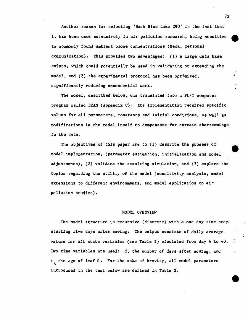
72
Another reason for selecting 'Bush Blue Lake 290 I is the fact that
it has been used extensively in air pollution research, being sensitive ~
to commonly found ambient ozone concentrations (Heck, personal
communication). This provides two advantages: (1) a large data base
exists, which could potentially be used in validating or extending the
model, and (2) the experimental protocol has been optimized,
significantly reducing nonessential work.
The model, described below, was translated into a PL/I computer
program called BEAN (Appendix C). Its implementation required specific
values for all parameters, constants and initial conditions, as well as
modifications in the model itself to compensate for certain shortcomings
in the data.
The objectives of this paper are to (1) describe the process of
model implementation, (parameter estimation, initialization and model
adjustments), (2) validate the resulting simulation, and (3) explore the
topics regarding the utility of the model (sensitiVity analysis, model
extensions to different environments, and model application to air
pollution studies).
MODEL OVERVIEW
The model structure is recursive (discrete) with a one day time step
starting five days after sowing. The output consists of daily average
values for all state variables (see Table 1) simulated from day 6 to 40.
Two time variables are used: d, the number of days after sowing, and
t ~ the age of leaf ~. For the sake of brevi ty, all model parameters
introduced in the text below are defined in Table 2.
.'
~
~
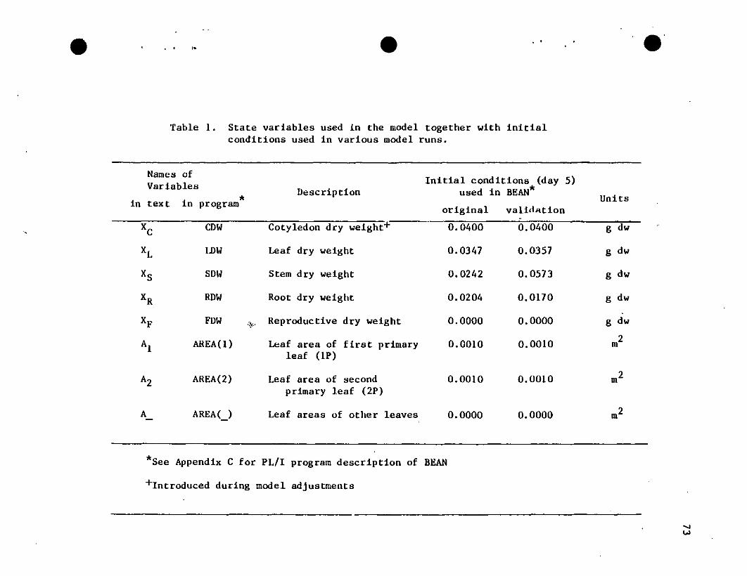
• ,. • . . .'Table 1. State variables used In the model together with initial
conditions used in various model runs.
Names ofVariables
in text *in programDescription
Initial conditions (day 5)*used in BEAN
original validationUnits
Xc
XL
XsXR
XF
Al
A2
A
CDW
lDW
SDW
RDW
FDW
AREA{l)
AREA(2)
AREAC)
Cotyledon dey weight~
Leaf dry weight
Stem dry weight
Root dry weight
.", Reproductive dry weight
Leaf area of first primaryleaf (lP)
Leaf area of secondprimary leaf (2P)
Leaf areas of other leaves
0.0400
0.0347
0.0242
0.0204
0.0000
0.0010
0.0010
0.0000
0.0400
0.0357
0.0573
0.0170
0.0000
0.0010
0.0010
0.0000
g dw
g dw
g dw
g dw
g dw
m2
m2
m2
*See Appendix C for PL!I program description of BEAN
+Introduced during model adjustments
"..,

T"ble 2 Parameters and ccnstants
Parameter or Occur- Source For thiaSubmodel Constant Description -, euce of the cultivar
Symbol in BEAN" eqn () value+ T
Incident PhAR at the top of the canopy &u:instein 10-2 sol)---
10 10 2 TS yes
Irradianca k K Extinction coefficient* (10-2 ) 2 1 yes
C - Fraction of leaf area in full irradiance 2 1 yes
a ALPHA Initial slope of the photosynthesis response curve*(ug C~ uEinat. -1) 3 2 no
Pn max: PM Maximum net photosyntnesis at saturation*(ug CO2 m-2 a·l ) 3 2 no, -
Daytime leaf res~iration rate*(ug CO2 m-2 sol)Photo:>ynthesis RL RL 3 2 no
e THETA Response curve shape parameter 3 2 no
'f PIlI Photo period (s dol) 4 T8 yea
1<.1 Growth respiration factor (g dw g c~O-l) 5 3 noRezpiration b Maintenance respiration factor (g C~O g dw-l ) 5 3 no
Allocation b ETA_ Partitioning coefficients* 5, 6, 7 T8 yes
p RHO Leaf area: dry weight conversion factor (of! g-l) 7 TS yes
Leaf M MM Sink. strength fUllction parameter 8 T8 yes
Distribution K KK Sin1<. strength function parameter 8 TS yes
B DB Sin1<. strength function parameter 8 T8 yes
r GAM/>L'l Leaf initiation/location matrix - TS yes
"see AppendiX C for description and listing of the PL/I computer program BEAN
'9:S~t11is study; l~L1eth (1982a); 2~atsl<.Y and Tiche (1980); 3..)1oldau and Karolin (1977).
*varies with time
• . .' • . , •.....po

•75
Once the state variables have been initialized, and all parameters
and constant values specified, the following cycle is followed until the
simulation is terminated [see Lieth (1982b) for detailed development]:...
1.) The vector A, containing values for the leaf area of each leaf
(m2), is used to obtain the cumulative leaf area vector F, as
follows:n
F = ... A (1)J, k=l:+l k
where the bottom leaf is indexed as 1 and the top most leaf as n.
2.) Available irradiance (~Einstein m-2 s-l) at leaf b is
where 10
is the incident irradiance at the top of the canopy, k is
the extinction coefficient on day d, F is the total leaf area oftot
the plant, and C is the fraction of Ftot exposed to full incident
irradiance (10),
•computed using:
IJ,(d).{~I -k(FJ,-CF tot)oe
for d<14
for FJ,<CF tot ' d~l4
for Fl,~tot, d~l4
(2)
(3)
3.) The It(d) values are used directly to compute the leaf gross
photosynthesis rate (~g CO2 m-2 9-1):
0'1 + Pn,max + RL - ~(O'Hi'n,max+RL)2 - 4aI6(Pn , max+RL)P8,t (d, tJ,)= ---.;...--...;,.---....;;.=;;;;...------.:~-
26
where a, P , RL, and 6 are parameters which vary asQt max
functions of leaf age. The amount of photosynthate produced by each
leaf is given by:
•Wl,(d) = P8,J,(d,tt)At(d)~.O.682.l0-6
where '¥ is the photoperiod (seconds) and 0.682 • 10-6 is the
conversion factor for ~g CO2 to 8 glucose •
(4)

76
4.) The net total amount of assimilate, W(d), produced by the plant
is determined by summing Wt(d) for all leaves (t) and accounting for 4Itrespiratory losses, i.e.:
Wt(d) = (l-kl)alt tWt(d) - k1b[XL + Xs + XR + XFJ (5)
where k1 and b are the growth and maintenance respiration factors.
5.) The partition coefficients, ~, control the allocation of
assimilates to the leaf (~L), stem (~S), root (~R), and reproductive
(~F) compartments. Letting these be a function of plant age (d), the
dry weights of the four compartments at time d+l are given by:
lb(d+l) .. yd) + b(d)W(d) (for 0- L, S, R, or F) (6)
6.) The incremental change in the leaf compartment (TIL(d)W(d»
is divided up over the leaves using the "leaf sink strength", St(d), a
measure of the relative activity of each leaf with respect to the
others. Assuming St.(d) to be proportional to the average growth rate,
and assuming a logistic growth pattern, the sink strength of leaf t on
day d can be written:
4It
=
1
il ij:l[ i+Be-k2M(tj+15
1
(7)
where B, k2, and M are parameters form the logistic growth function.
The change in leaf are of leaf t is determined by:
A.e (d+l) .. At (d: + 'T1L(d). W(d)St (d)p
where p is the ratio of le~f area (m2) per gram dry weight.
7.) Information on initiation of new leaves and their location
(8)
within the canopy is taken from a table (hereafter called r) built into
the computer model.
8.) Return to step 1 with day set to d+l.4It
•77
METHODS AND MATERIALS
Experimental Design
All experimental work was performed at the Southeastern Plant
Enviromnent Laboratory during the spring and summer of 1981. The design
consisted of two sets of plants (P. vulgaris L. cv. 'Bush Blue Lake
290') grown in succession, (Phase A and B) each with the same growth
conditions: 9 hour days at 26° C and 15 hour nights at 22° C: 60-80%
relative humidi ty; 590 1J E m-2 s-l incident irradiance at the top
of the canopy: a.watering scheme of nutrient solution in the morning and
deionized water in the afternoon, each administered to the drip point.
Beans were sowed into 250 ml styrofoam cups at 4 seeds per cup. On
day 8 (after sowing) the seedlings were transplanted into 15.2 em
• diameter pots. The harvest days were: days 5, 8, 11, 14, 18, 22, 26,
30, 34, and 38. At each harvest, four plants were dissected into leaf,
•
stem, root, and reproductive portions in order to obtain their fresh and
dry weights. Roots were washed gently in lukewarm water.
Both phases were used to determine canopy characteristics. The data
collected from the first set of plants consisted of leaflet areas, fresh
weights and lengths. Each leaflet was identified as to its leaf
identity on the plant (see AppendiX A). The same scheme was used with
the second replication while collecting leaf lengths and leaf heights
above the soil surface: PAR (photosynthetically active radiation) levels
at each leaf were measured using a Lambda Instrument Company LI-185
quantum meter: for each plant those leaves just beginning to expand were
noted with their leaf codes •

78
Determination of Model Parameters and Constants
The model contains a number of parameters and constants whose
evaluation is critical to the usefulness of the model. These are
summarized in Table 2 and methods for their. evaluation are described
below.
a. Irradiance SUbmodel
The irradiance submodel is described by Lieth (1982a). 'For
e.
k = A + B/Ftot
Here A = 7.63 and B = 2.23; C from eqn (2) was set to 0.167 (Lieth,
1982a).
b. Photosynthesis Submodel Parameters
The photosynthetic parameters Of, Pn max' RL' ·and 6 we"re,
(9)
e
estimated from the photosynthesis response curves for various plant ages
presented in Catsky and Ticha (1980, Fig. I, p. 394). For each graph,
the parameters were evaluated using the methods described in Appendix B
and the resulting values plotted against t (leaf age, see Fig. 1). The
following empirical equations were fit to these data using the Marquardt
nonlinear regresssion algorithm (Marquardt. 1963) of the Statistical
Analysis System (Helwig and Council, 1979).
The initial slopes of the photosynthesis response curves, Of [Fig.
1(a)J are:
which represents a curvilinear increase (quadratic) up to its maximum at
(10)
e

•
•
a
1.4
1.2
1.8
S
(a)
18
18
•
•
•
T (DAYS)
•
IS
IS
•
•
28
•
28
79
•Figure 1. Plots showing the variation of the photosynthesis parameters
(a) a, (b) Pn,max, (c) RL, and (d) 6, with time. The solidlines are the empirical functions fitted to the data.

•
80
•
.1 IS
•• .. ••
• • •• • •
e
1.75
1.7
(c)
(d)
••
•
•
•
•• •
•
•
T (/)AYS)
Figure 1. continued. •

• age t a (~al/2a2)' and a linear decline thereafter •
the coefficients are presented in Table 3.
The value of
81
for t ~ tp
for t < t p
Note that t p was fixed to be the value of t where the quadratic
branch has its maximum (-b l /2b 2).
The day-time respiration rate of the leaves, RL, [Fig. l(c)] is
modelled by a decreasing quadratic section followed by a constant whose
•
The maximum net photosynthetic rate P , is represented by a, n,max
linear increasing branch (for t < t p) and a curvilinear decrease-
(quadratic) for t ~ t p :
(
m2(t_tp) + bO + bItp + b2~Pn max(t)= 2
, bO + bIt + b2t
The least squares fit to the data in Fig. l(b) is given in Table 4.
value is the minimum of the quadratic branch:
{CO + CIt + c t 2 for t < t R2~(t) =
forc3 t ~ t R
Here t R is the leaf age at which the minimum of the quadratic branch
occurs. This implies:
and:
c3 = Co + cltR +2
~ Co - cl/2c2
As a result, only cO' cI' and c2 needed to be estimated (see
Table 5).
9, a dimensionless parameter related to the shape of the
(11)
(12)
•photosynthesis response curve (see Appendix B) is modeled using a
constant function, since the data [Fig. led)] show no clear trend. Thus
9 = 0.9435, the average value, is used.

Table 3. Values of the coefficients of a(t) [eqn (10)J.
82
•Coefficients
value
ao-0.617
a1
0.281
a2
-0.00949
.m1
-0.164
t
14.8
Table 4. Values of the coefficients of Pn,max(t) [eqn (11)].
Coefficients bO b1 b2 m2 t p
value 214 167 -7.92 219 10.5 •Table 5. Values of the coefficients of RL(t) [eqn (12)).
Coefficients
value
Co1960
C1
-334
c2
15.8
tR
10.6
•
•
•
83
The photoperiod (~) is set at 32400 seconds per day, representing 9
hours of irradiance.
c. Respiration Submodel Parameters
The respiration model developed by McCree (1970) has been widely
applied and, thus, estimates for the parameters k 1 and b [eqn (5)]
are available for many different species (see Hunt and Loomis, 1979).
These studies place a range on band k 1 of .0016 to .016 and .20 to .35,
respectively, for higher plants (Thornley, 1976; Hunt and Loomis, 1979).
Values of .014 for band .25 for k 1 were found by Moldau and Karolin
(1977) for Phaseolus vulgaris in experiments carried out at 25°C.
d. Allocation Submodel Parameters
The partitioning coefficients, ~ n_ TL and TL''L' ''S'R' ''F'
determine the proportion of the available assimilate allocated to each
compartment. Various physiological events indicate that these do vary
with the ontogeny of the plant. The onset of reproductive growth, for
instance, involves a change in the allocation scheme with assimilate
being utilized by the reproductive compartment.
The partitioning eoefficients were estimated from dry weight
increments between harvests of the various plant parts. The ~'s were
obtained by dividing each such increment by the total dry weight
increment; this process assumed that the conversion efficiencies were
the same for all compartments, so that the proportions allocated were
equal to the proportions of materialized dry weight. It was noted that
the sum of the increments of leaf and reproductive dry weight made up
roughly half of the total increment over the entire observed ontogeny
(Fig. 2). Mathematically, this means:• i1t. + ~ = 0.5 (13)

84
••
•s 18 16 a
IMY
2Ii sa
Figure 2. The ratio of "leaf and reproductive dry weight increment"to "total plant dry weight increment", E, (symbol CI )plotted against plant age (~Y). The values' closeproximity to 0.5 indicates that approximately half of theassimilate is allocated to the leaf and reproductivetissue.
•

85
•and since the ~'s sum to 1:
'11S + '!la = 0.5 (14)
The individual estimates of the '11's, however, vary with the age of
the plant (Fig. 3). A set of empirical equations were formulated to
simulate these values for use in the model. Obviously, ~ = 0.0 for the
time prior to flowering (t < 24) so that 1lt • 0.5 for this time. A
declining trend was noted for nL
for t > 24, so that, assuming this
trend to be linear, the equations:
•and:
~.{0.5
0.5 - (d-24)/36
0.0
(d-24) /36
for d < 24
for d ~ 24
for d < 24
for d ;;, 24
(15)
(16)
were obtained [Fig. 3(a) and (b»). The estimates for stem and root
partition coefficients exhibit increasing and decreasing linear trends,
respectively, until well past the flowering date, with no discernable
pattern thereafter [see Fig. 3(c) and (d»). The day for the change was
assumed to be "podfill", about day 30. As with ~ and ~ continuous
functions were used to represent the data:
'11S 2 {
0.32(d-l)/26 for d < 30
0.32 for d ;;, 30
and:
{ 0.5 - 0.32(d-l)/26 for d < 30
'!la"for d ;;, 300.18
(17)
(18)
•e. Leaf Distribution Submodel Parameters
A straight line through the origin provided a good description for
the relationship between leaf area and leaf dry weight (Fig. 4). This
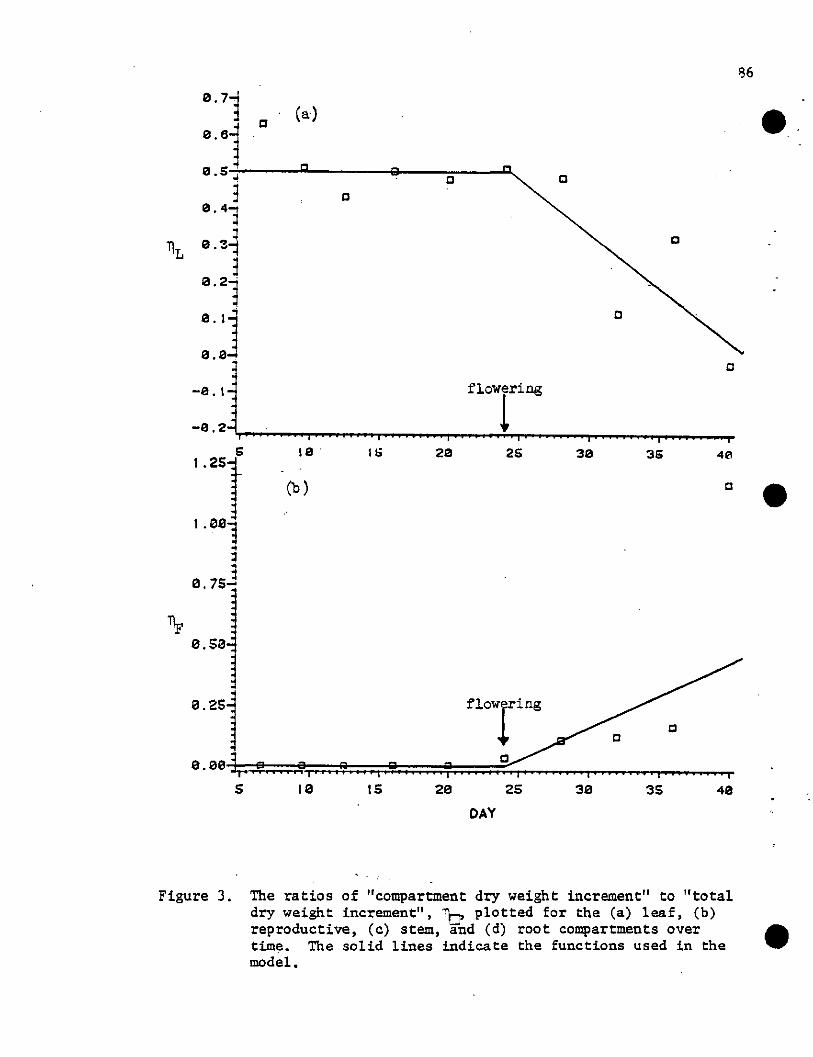
136
0.71a (a) •0.61
0.5 ..C C
3 c0.41
J a'ilL 0'~1
30.21
0. I] C
0.0C
-0. I flOWrring
-0.2
5 10 . lli 20 25 30 36 40
1·2S1 (b) c •1. e01~
e. 7sJ
Tir0.50
0.251 flowfing
ac
0.09 a: 4 i i C ii' i i' :: i· , , 4 i i 4 i , i
S 10 IS 20 25 30 35 40
DAY
Figure 3. The ratios of "compartment dry weight increment" to "totaldry weight increment", U plotted for the (a) leaf, (b)reproductive, (c) stem, and (d) root compartments over •time. The solid lines indicate the functions used in themodel.
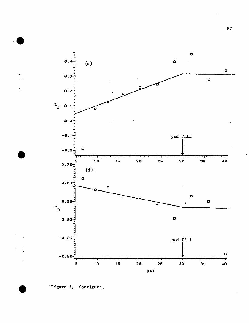
-0.25 pod fill
1 0-(l.S0
5 !3 IS 2e 25 30 35 ...eDAY
• . Figure 3. Continued•
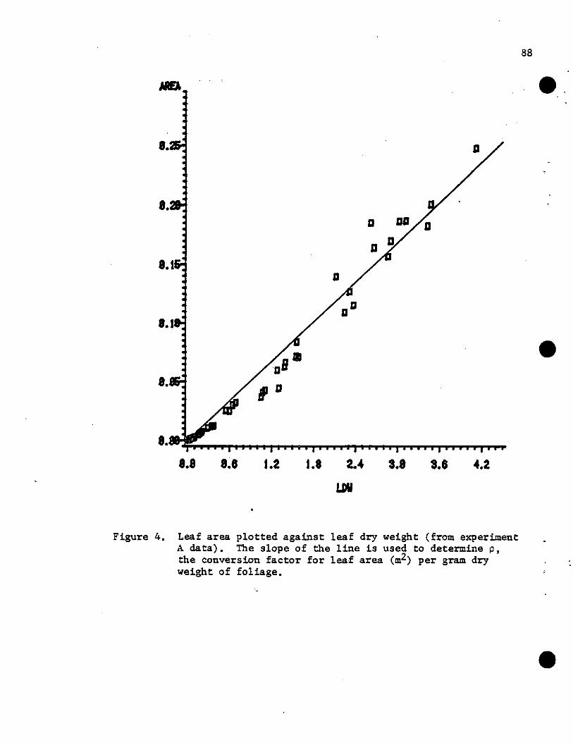
88
•
'.1
II •DB8.
I D
8.
8.8 8.8 1.8 2."1.DII
3.8 3.8 ".2
Figure 4. Leaf area plotted against leaf dry weight (from experimentA data). The slope of the line is used to determine p,the conversion factor for leaf area (m2) per gram dryweight of foliage.
•

•
•
•
89
meant that P, the ratio of leaf area (m2 ) per gram dry weight, the
slope of this line, was constant over time. The value of p, determined
using a linear least squares routine (with intercept fixed at 0), was
0.0563 (a2 • 0.98).
The leaf sink strength function parameters, k2 ' B, and M, were
estimated from data reported by Da Silva (1981) for a time series of
leaf areas measured entirely for the same leaf. Since eqn (7)
represents the normalized average rate of change of the logistic
function,the parameters can be determined by fitting this equation to
Da Silva's data (Fig. 5). This results in the following parameter
values: M • 88.8, B • 21.0, and k2
• 0.00360.
The leaf initiation matrix provides the leaf distribution within the
canopy by providing the leaf height-ranking in the canopy and the leaf
initiation dates. The leaf initiation information was collected in
phase B of the experimental work, (third column, Table A-l, Appendix A).
These data, together with the knowledge of which leaves were present on
given days (fourth column, Table A-l, Appendix A) allowed the estimation
of dates on which a given leaf was most likely to start unfolding
(column 2, Table 6). The ordering (index, Table 6) corresponds to the
sequence in which they were initiated.
The second column of r (column 3, Table 6) represents the ranking of
the locations of the leaves in the canopies. Lower values indicate
lower levels in the canopy. These values were obtained from
observations of canopies of plants of phase B, as follows: The main
stem leaves and the first leaf on the fourth trifoliate lateral branch
were always in a fixed order: lP, 2P, IT, 2T, 3T, 4T, ST, 4TI. The
remaining lateral trifoliates found most commonly (lPI, IP2, IP3, 2PI,

•90
• ••
•••• •~ • •
C\JS •"~ •al *<Il... *al
""'al *S
•*
5 7 9 1\ 13 15 17 19 21 23 25 •Leai' age (days)
Figure 5. The plot of the leaf area of the first trifoliate with time(*. from Da Silva, 1981) with the logistic ~quation fittedto the data (solid line).
•

•
•
•
•
Table 6. The values of the elements ofthe matrix r with theircorresponding leaf codes.
rIndex Leaf codes
col.1* col.2
1 3 18 1P-2 3 17 2P
3 10 16 1T
4 13 13 2T
5 15 11 3T
6 16 15 1P1
7 17 12 1T1
8 18 8 4T
9 20 14 2P1
10 22 5 5T
11 24 10 1T2•
12 25 I 7 2T1I
13 26 I 6 1P2I
14 28I 3T1I 9
15 30 I 1 1P3I
16 31 I 2 1T3•17
I4T132 I 3
18 34 I 4 3T2I
*day after sowing on which leaf emerges
91

92
lTl, lT2, lT3, 2Tl,.and 3Tl) were ordered in between these by
approximating all average leaf heights. An additional leaf was added
(3T2) to bring the total number of leaves in the model in line with the
observed number (18) for the mature (day 38) plant.
Model Adjustments
During model implementation, two problems were noted, requiring
major adjustments: (1) the dry weight increments were much smaller than
evident in the experimental data, and (2) the leaf photosynthesis model
did not follow the same pattern as found by Da Silva (1981) for the
•
cultivar used here. These two problems were dealt with, respectively,
by (1) building a compartment into the model to represent the seed
cotyledon and (2) making adjustments in the photosynthesis submodel for •
temperature and cultivar differences.
a. Seed Cotyledon Compartment
In searching for an explanation for the slow increase in growth
during the early stages of the simulation, it was noted that the plant
has a seed cotyledon from which to obtain assimilates during the first
few days of its ontogeny. Unfortunately, no data was collected
regarding this factor, as seed cotyledons were not weighed separately.
Nonetheless, a fifth compartment was included to represent these. It
was assumed that 0.04 grams of the measUred stem dry weight (day 5) was
seed cotyledon, and that its depletion was at a constant rate y. The model
allowed no infusion of substrates into this compartment. In the present
version of the model y was set to 0.08 (g day-i).
Furthermore, the rate of photosynthesis in the cotyledons was
assumed to be the same as in the leaves. Eqn (3), with the parameter •

•
•
•
93
values noted above, was used. A constant leaf area of 0.0003 m2 was
assumed.
b. The values of the photosynthesis parameters a, Pn,max' RL' and ewere determined from data presented by catsky and Ticha (1980) and
hence, represent their cultivar, growing in their e~vironmental
conditions (24·C). In an attempt to conform these results to the
present conditions (26·C), the temperature dependence of Pg,max
presented by Tenhunen et al. (1976 a and b) fer Phaseolus vulgaris was
used. A temperature increase of 2°C from 24·C was found to increase
Pg,max by 14%. Thus, a correction factor of 1.14 was used for
P + RL (line 2875 of BEAN, Appendix C).g,max
Furthermore, in using the photosynthetic control curves presented by
Da Silva (1981) for the present cultivar, it was noted that the
physiological time scales of the two cultivars did not coincide. This
was due to the following two reasons: (1) the time variable in the
model is "leaf tissue age" whereas in Catsky and Ticha's paper it is
"day after sowing", a difference of 5 days for the primary leaves, and
(2) a comparison of the trends in the photosynthetic rates over the
ontogeny of the plants indicated that the present cultivar developed
substantially slower (30-40%), possibly due to the shorter photoperiod.
As a consequence of these facts, it was deemed justified to use the time
transformation 2(t+5)/3 in the photosynthesis submodel (Line 2710 of
BEAN, Appendix C).
Programming considerations
All programming for determination of the parameter values was
accomplished using the Statistical Analysis System. The model
implementation is in PL/I (see Appendix C).

•94
RESULTS AND DISCUSSION
Model Behavior
The results of the 40-day simulation for an average plant in the.
canopy are presented in Figs. 6-8. The shapes of the resulting model
output. curves follow the pattern in plant part dry weight data quite
well, even though the actual dry weight predictions are often not within
the 95% confidence intervals of the mean values for each day (see Fig.
6). The model predictions for stem and reproductive organs [Fig. 6 (b)
and (d)] appear to follow the experimental data more closely than the
predictions for the leaf and root organs [Fig. 6 (a) and (c)]. The
total dry weight is underpredicted, especially for days 18 through 27
[Fig. 6 (e)].
The dynamics of the model can be best analyzed by comparing the •
model output curves for each plant organ with one another (Fig 7). The
relative proportion of leaf : stem : root : reproductive dry weights on
day 38 for the model is 33:29:21:17 compared with 37:25:27:11 for the
experimental data. This, together with the previously noted growth
patterns shown in Fig. 6, indicates that the overall behavior of the
model is quite good.
The gross and net photosynthesis and respiration rates for the
entire plant reached their maxima at days 40, 39, and 42 (Fig. 8) at
rates of 0.722, 0.456, and 0.275 g glucose days-I, respectively.
Table 7 lists the daily summaries throughout the ontogeny of the plant.
A typical page of output from the computer program (Appendix C)
includes a complete canopy profile (as in Table 8) allowing comparison
of various aspects of the canopy: 1) The predictd available PAR •
declines in roughly the same manner throughout the canopy as the

•95
•
Ca)
• 'i' Ii'" Ii. I' 4" : Ii" i
8 5 18 IS 2:3
DAY
2S ss
•
. Figure 6. Model predictions for (a) leaf, XL, (b~ stem, XS' (c) root,XR, (d) reproductive, XF, and (e) total, tx, dry weights(g) compared against the data means with 95% confidenceintervals •

.:L_.........~iI~;;;;:;:;;~l:.:..~i~i:i:i:, :'1~i:i:i:':.:":9'TT"i' ,. $, ., i •• ; ,.' j '$ 'i' ,:,.u•••• u", , u. ,Ui
(b)
•
•96
3S382S28IS18s
t.
2.
2.
3.
3.
(c)
f
,,: l" Ii' Ii." hi"'" t Ie tC i ilii' I' Ii Ii. i. i i' Ii' i"" i
8 S fa IS 28
DAY
25 •Figure 6. Continued.

l' hOi , u.. ji' II .. u" i $ Ii". eo Ui
•
•
I.
I.
I.
I.
9.
9.
a.
e
(d)
-S 18 IS 28 2S 3S
97
3S2S23
DAY
\SIIIs
(e)
·Continued.
ea.~l.."'""""'·~;;;;::;;:;:;=~':':'i~i~':I~":':"'i"'ii'i'i"'iiii' 111 •• 11"""."1":""",
2.
S.
7.
la.
\2.
Figure 6.
DC·l l
•

98
•
•
ow3. S '
2. FL
2. R
6 18 16 28 2&
DAY
38
Figure 7. Model behavior of the four plant part dry weight (g). DW.compartments. Xo-
•

•99
PS'tN, 8.7
8.Pg
•
6 II 16 28 26
DAY
•
Figure 8. Model predictions of the whole-plant daily gross (Pg) andnet (Pn) photosynthesis and respiration (R).

Table 7. Simulation R~sults
100
••Ca:lpartI!>.nt Dry Weights (g) Carbohydrate Rates
(g glucose darl )
DAY LDW S!Ili R!Ili FDW T!Ili PSYNTHTE NETASIML RESPLIlTN
6 0.041 0.025 0.026 0.000 0·092 0.019 0.013 0.0067 0.050 0.026 0.034 0.000 0.110 0.026 0.018 0.0088 0.061 0.028 0.042 0.000 0.131 0.031 0.021 0·0099 0.076 0.031 0.055 0.000 0.162 0.044 0.031 0.013
10 0.098 0.036 0.072 0.000 0.206 0.061 0.044 0.01711 0.126 0.043 0.093 0.000 0.261 0.077 0.055 0.02212 0.163 0.053 0.120 0.000 0.336 0.105 0.076 O.O~
13 0.217 0.069 0.158 0.000 0.444 0.147 0.106 0.04114 0.252 0.080 0.182 0.000 0·514 0.102 0.071 0.0311; 0.292 0.094 0.208 0.000 0·594 0.115 0.080 0.03516 0.340 0.112 0.238 0.000 0.690 0.136 0.095 0.04117 0.389 0.131 0.268 0.000 0.788 0.143 0.099 0.04418 0.442 0.153 0.299 0.000 0.894 0.153 0.106 0.04719 0·503 O. 100 0·333 0.000 1.016 0.177 0.122 0.05520 0.572 0.212 0.370 0.000 1.154 0.200 0.138 0.06221 0.649 0.250 0.409 0.000 1·308 0.223 0.154 0.06922 0.729 0.292 0.447 0.0...-0 1.468 0.233 0.160 0.07323 0.821 0.342 0.490 0.000 1.653 0.268 0.184 0.08424 0·920 0.398 0.;33 0.000 1.851 0.290 0.198 . 0.09225 1.030 0.465 0.579 0.006 2.080 0·331 0.227 0.10426 1.140 0.544 0.629 0.021 2.334 0.375 0.257 0.11827 1.260 0.638 0.681 0.045 2.624 0.427 . 0.293 0.13428 1.380 0.733 0.735 0.078 2.926 0.436 0.297 0.13929 1. ;00 0.1>37 0.793 0.123 3.253 0.480 0.326 0.15430 1.610 0·949 0.856 ~.181 3.596 0.;15 0·349 0.16631 1.730 1.070 0·924 0.255 3.979 0.561 0·379 0.18232 1.840 1.200 0.998 0.346 4·384 0.605 0.400 0.19733 1. 950 1.340 1.080 0.455 4.825 0.651 0.438 0.21334 2.040 1.470 1• 150 0.570 5.230 0.625 0.413 0.21235 2.130 1. 61 0 1.230 0.704 5.674 0.667 0.440 0.22736 2.210 1.760 1. 310 0.857 6.137 0.695 0.456 0.23937 2.270 1.900 1·390 1.010 6.570 0.677 0.437 0.24038 2·320 2.040 1.470 1.190 7.020 0.706 0.454 0.25239 2.350 2.190 1.550 1.380 7.470 0.716 0.456 0.26040 2.380 2·340 1.640 1·580 7.940 0.722 0.455 0.26741 2·390 2.480 1.720 1.800 8.390 0.720 0.449 0.27142 2·390 2.620 1.800 2.010 8.820 0.714 0.439 0.27543 2·390 2.750 1.870 2.220 9.230 0.680 0.408 0.27244 2·390 2.870 1·940 2.410 9.610 0.648 0·380 0.26845 2.390 2·980 2.000 2·580 9·950 0.613 0.349 0.264
•
•

• • •
Table 8. Canopy prorile (model output) ror day 38
Lear Incident Gross Photo- Gross Photo- sinkLeaf' AgeAr~a PAR synthe~is synthate
In (days) (m ) liE m- 2 s-l /Jg CO2 m- s-l g glue. day-l strength
lPJ 8 0.0036 590 559.78 0.0399 0.136In 7 0.0029 590 559.78 0.0319 0.1264Tl 6 0.0023 590 48j.I6 0.0216 0.1123T2 4 0.0014 590 384.64 0.0102 0.0785T 16 0.0091 590 796.07 0.1584 0.049IP2 12 0.0067 590 739.77 0.1039 0.1122Tl 13 0.0074 328 444.41 0.0700 0.0964T 20 0.0103 2'/6 342.'75 O. (1180 0.0163'r 1 10 0.0051 216 264.62 0.0277 O. U6lT2 14 0.0081 192 263.90 0.0457 0.0793T 2j 0.0106 159 148.32 0.0346 0~006
1TI 21 0.0105 124 135. J6 0.0312 0.0122T 25 0.0106 96 58.50 0.0137 0.0032PI 18 0.0099 74 106.0> 0.0230 0.0281P1 22 0.0106 59 55·05 0.0128 0.009IT 28 0.0106 46 12.91 0.0030 0.0012P 35 0.0093 35 0.00 0.0000 0.000lP 35 0.009'j 28 0.00 0.0000 0.000
Total 0.1383 0·7056 1.000
....0....

102
measured trends. 2) The largest leaves in the canopy (model) are the
lower mainstem trifoliates (IT, 2T, 3T, and 4T) and the first two
lateral trifoliates (lPl and ITl) as is the case in the actual plants,
although the leaf area values are in some cases only 35 to 40% of the
observed values. This is probably due to the fact that the model does
not incorporate the fact that leaves in full light, producing at the
highest rates, in fact get more photosynthate than leaves in lower light
with the same sink strengths. 3) The sink strength values of zero for
IP and 2P indicate that the simulator has "dropped" these leaves, a
situation which is observed in the experiments. The first mainstem
trifoliate (lTl) is "dropped" by the simulator on day 42; 50% of the
experimental plants are in the process of discarding this leaf on day
38.
Validation
The term "valid" has many different meanings in the modeling\
literature, ranging from definitions which allow most "reasonable"
models to be classified as valid (van Horn, 1971) to definitions which
allow virtually no model to be so classified (Mankin et al., 1975).
Many authors avoid the word "validate" because of its inherent "roots of
ambiguity" (Caswell, 1976) and instead assign specific definitions to
words like "confirmation", "verification", "usefulness", "adequacy" and
"reliabililty" (Naylor et al., 1966; Mihram, 1976). In this discussion,
the terminology of Mihram (1976) will be used for "validation", i.e.,
analysis of "the adequacy of the model as a mimic of the system which it
is intended to represent". Thus, the basic objective of the validation
study presented here is to compare the predictions of the BEAN model to
•
•
•

•
•
•
103
the observations made on certain attributes of snap bean growth. For
this purpose, the data used in the development of the model may not be
used in the validation, as this would represent a cyclic argument.
Hence, it was necessary to obtain an independent data set.
a. Validation data set,
The validation data set was obtained under the same conditions as
those experiments carried out for parameter estimation. Harvests were
taken on a slightly different schedule: days 5, 8, 12, 15, 18, 21, 24,
27, 30, 34, and 38. At each sampling date, leaf, stem, root, and
reproductive dry weights were obtained.
b. Validation methods
In order to compare the model to experimental observations the dry
weight predictions for each compartment were compared with the mean
values of the plant part dry weights for each day. To perform the
needed statistical tests, it was necessary to make some assumptions
about the error structnre of the data. A frequently used assumption in
plant growth analysis'is that of lognormally distributed error (Causton
et al., 1978); his assumption would mean that the data distribution for
each day would be skewed. In both the validation data, as well as the
parameter estimation data, such skewness was not observed. Thus, it was
assumed that the data on any particular day were normally distributed
with time dependent variances. This allowed testing the null hypothesis
that the model prediction for day d was equal to the true mean for day d
using a t-test. For practical purposes, this was the same as
determining whether the model prediction fell within confidence
intervals of the mean. Thus, plotting the 95% confidence intervals of
the means together with the model prediction curve provided a method
for carrying out all tests at once~

c. Validation results and discussion
The initial conditions arising from the validation data are given
104
•in
Table 1.
The resulting model behavior (Fig. 9) shows a fit similar to Fig. 6.
From the point of view of hypothesis testi~ the model is an adequate
representation of reality, in the sense of Mihram (1976), since there
are many model predictions which cannot be said to be significantly
different from the means, especially for the stem, root, and
reproductive compartments. The percentages of tests in which the null
hypothesis (model prediction for day d • mean for day d) could not be
rejected, are 30% for the leaf dry weight, 70% for the stem and root dry
weights, 80% for the reproductive dry weight, and 60% for the total dry
weight.
Recommendations for Future Work
Most modeling studies consist of a number of immediate and extended
goals. The immediate goals are sttended to during model development,
while the secondary goals are pursued after accomplishing the primary
goals. Since pursuing secondary goals can often entail extensive model
modifications, it is imperative that initial model development proceed
with future interest in mind. In the present study the primary
objective was to develop a plant growth model for Phaseolus
vulgaris L. cultivar: 'Bush Blue Lake 290' whereas the secondary goal
was to utilize the resulting model in gaseous air pollution studies.
These studies include phytotron, greenhouse and field experiments with
•
varying combination of gaseous pollutants. In order to modify the mOdel.
to handle such a diversity of conditions, the sensitivity of the model
to changes in the parameters and submodels must be understood.

•105
(a)
XL
I I II
•8 5 18 15 28 2S 38 35 43
DAY
Figure 9. Validation data (means with 95% confidence intervals) withmodel predictions for (a) leaf, ~. (b) stem, Xs. (c) root.XR• (d) reproductive. XF• and (e) total. tx. dry weights(g) compared over time (~Y).
•

2.
Xs
2.
2.
I.
I.
e.
2.
(b)
S
(c)
13 IS
•
2S 38 49
106
•
•
•35
I
25
...
2ll
DAY
. ISS 188
l.
i--a. ..,..........,..........""-""'"....................................,.,...,...................,..................,.....,........................~
9.
Figure 9. Continued.

9.
9.
XF
9.
9. +X)
• 19 -9 5 19 15 2S 25 38 35
I107
I
• I.
(d)
I.
8 (e),
"rrOTTOTT~~nMM~~TTTTTTTTT"'''~iJI'''i'TTTT1'iiii'''J:''''ii'il·i'i'ii' 'I
I
•
6
l:lC.i J.
2
II
Figure 9.
-----,j,S Ie
Continued.,
IS 2ll
OI.Y
2S 49
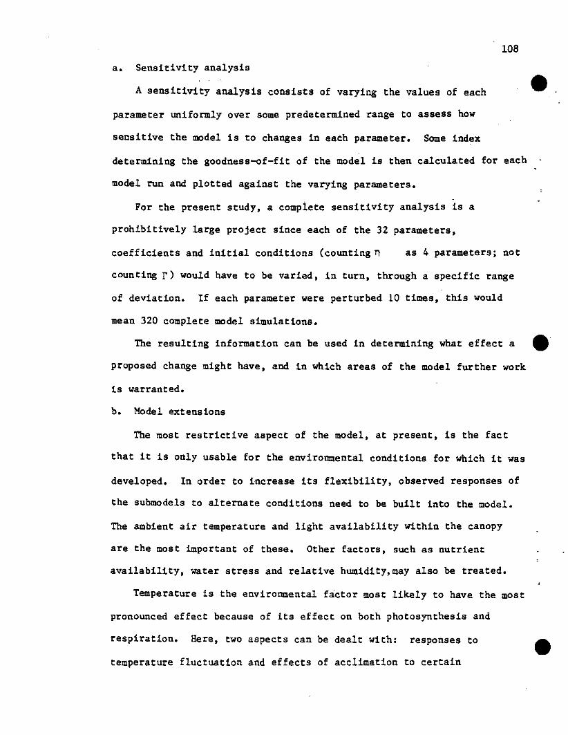
108
a. Sensitivity analysis
A sensitivity analysis consists of varying the values of each
parameter uniformly over some predetermined range to assess how
sensitive the model is to changes in each parameter. Some index
determining the goodness-of-fit of the model is then calculated for each
model run and plotted against the varying parameters.
For the present study, a complete sensitivity analysis is a
prohibitively large project since each of the 32 parameters,
coefficients and initial conditions (countingn as 4 parameters; not
counting r) would have to be varied, in turn, through a specific range
of deviation. If each parameter were perturbed 10 times, this would
mean 320 complete model simulations.
The resulting information can be used in determining what effect a
proposed change might have, and in which areas of the model further work
is warranted.
b. Model extensions
The most restrictive aspect of the model, at present, is the fact
that it is only usable for the environmental conditions for which it was
developed. In order to increase its fleXibility, observed responses of
the submodels to alternate conditions need to be built into the model.
The ambient air temperature and light availability within the canopy
are the most important of these. Other factors, such as nutrient
availability, water stress and relative humiditY,may also be treated.
Temperature is the environmental factor most likely to have the most
pronounced effect because of its effect on both photosynthesis and
respiration. Here, two aspects can be dealt with: responses to
temperature fluctuation and effects of acclimation to certain
•
•
•

•
•
•
109
temperature regimes. The latter is a very important problem since
acclimation regimes are difficult to quantify and thus, present
intriguing possibilities for extending this model. Responses to
temperature fluctuation, on the other hand, are better understood. For
example, Tenhunen et al. (1976b, pp. 112-113) showed that the
photosynthetic response to temperature developed by Johnson et al.
(1942) could be applied to bean leaf photosynthesis models by making the
gross photosynthetic maximum (P + RL) a function ofn,max
temperature.. It should be noted that their development is for leaf
instead of ambient air temperature, making it imperative that a
correlation between these two variables be developed. The respiration
submodel would also have to be modified to predict the response to
changing temperatures. It would be hoped that the model. would predict
patterns observed (Wilson and Ludlow, 1968) for bean leaf growth under
different temperatures.
The distribution of photosynthetically active radiation is also
likely to be different outside the phytotron. In greenhouses, diurnal
light variations exist so that a submodel for 10
, the incident
radiation at the top of the canopy would have to be built into the light
submodel. Under field conditions, thiS, in addition to other
considerations like row spacing, light angle, etc., would have to be
considered •
In studies involving water and nutrient relations, the model would
have to be substanstially modified to incorporate the root physiology of
the plant. In the present setup of the model, this is not likely to be
worthwhile since the basic carbon flow system would also have to be
altered to include the flow of nitrogen and water, requiring a
completely different model development.

110
The primary long-range goal was to develop a modeling tool for
testing hypotheses regarding the effects of air pollutants on the growth
and development of snap bean plants. ,This goal cannot yet be realized
for two reasons: 1) the model adjustments corresponding to the
c. Application in air pollution studies
hypotheses being tested cannot be made intelligently without the
sensitivity analysis and 2) the individual submodels need to be
validated prior to using their results by themselves. Further work on
the partitioning aspects of the model (discussed above) should also be
done prior to using the model to test hypotheses.
Of the many effects of air pollutants on plants (see Horsman and
••
Wellburn, 1976) the inhibition of apparent photosynthesis has drawn a
lot of attention (Todd, 1958; Bennett and Hill, 1973; Capron and •
l1ansfield, 1976). Ozone in· particular has been implicated in many of
these; yet there is no consensus on the mechanism of injury (see Heath,
1975 and 1980, for reviews). Many different hypotheses have been
modeled (Bennett et al., 1973; Steinhardt et al., 1976; O'Dell et al.,
1977; Unsworth, 1980; Tingey and Taylor, 1981) yet none of these have
been built into simulators to see if they will mimic the observed
effects. This is the main area where the present model can be of
service. For example, the reduced chlorophyll level due to episodic
03 exposure reported by Craker and Starbuck (1972) for Phaseolus
vulgaris would imply proportionately reduced gross photosynthesis rates.
It would be interesting to see whether this reduction results in the
same observed changes in growth patterns as predicted by the model.
Similarly, effects on respiration and dry matter partitioning could be •
investigated.

•
•
•
III
CONCLUSION
The model for the growth and canopy development for snap bean
presented above is a valid simulator for the dry weight of the plant
parts throughout the life cycle of the plant. This waa shown in
particular for the cultivar Phaseolus vulgaris L. cv. 'Bush Blue Lake
290' grown under controlled conditions. Data was collected for
parameter estimation of the light attenuation, carbohydrate allocation,
and leaf distribution submodels. The photosynthesis and respiration
parameters were developed from information on Phaseolus vulgaris (other
cultivars) in the literature.
Further development of the model, to allow its utilization as a
hypothesis testing tool in air pollution studies, is possible as soon as
the sensitivity analysis and submodel validation sre complete.
Extensions to field studies may be possible but will require extensive
modifications.

112
REFERENCES
Bennett, J. H., Hill, A. C., and Gates, D.gaseous pollutant sorption by leaves.23, 957-962.
M., 1973. A model forJ. Air Poll. Contr. Assoc. •
Capron, T. M. and Mansfield, T. A., 1976. Inhibition of netphotosynthesis in tomatoe in air polluted with NO and N02• J.Exper. ~. 27, 1181-1186.
Caswell, H., 1976. The validation problem. In: Systems Analysis~Simulation ~ Ecology, Vol. IV ed. B. C. Patten, pp. 313-325.Academic Press, New York.
Catsky, J. and Ticha, I., 1980. Ontogenetic changes in the internal,limitations of bean leaf photosynthesis. 5. Photosynthetic andphotorespiration rates and conductances for C02 transfer asaffect by irradiance. Photosynthetica 14, 392-400.
Causton, D. R., Elias, C. 0., and Hadley, P., 1978. Biometrical studiesof plant growth. I. The Richards function and its applications inanalyzing the effects of temperature on leaf growth. 11.~.
Environ. I, 163-84.
Craker, L. E. and Starbuck, J. S., 1972. Metabolic changes associated ~with ozone injury of bean leaves. ~.~. Plant~. 52, 589-597.
Da Silva, E. A. M., 1981. Correlation of Various Developmental andPhysiological Variables of Phaseolus vulgaris L. 'Bush Blue Lake290' with Ozone Sensitivity. Ph.D. Thesis, Department of Botany,North Carolina State University, Raleigh, NC.
Dell, R. A., Taheri, M., and Kabel, R. L., 1977. A model for uptake ofpollutants by vegetation. J.!!!. Poll. Contr. Assoc. 27,1104-1109.
Heath, R. L., 1975. Ozone, In:eds.: J. B. Mudd and T. T.New York.
Responses of Plants to Air Pollution,Kozlowski, pp. 23-55,""Academic Press,
Heath, R. L., 1980. Initial events in injury to plants by airpollutants. ~. Rev. Plant Phys 31, 395-431.
Heck, W. W. Personal communication.
Helwig, J. T. and Council, K. A., 1979. The SAS User's Guide. SASInstitute, Inc. P.O. Box 10066, Raleigh, NC.
Horsman, D. C. and Wellburn, A. R., 1976. Appendix II. Guide to themetabolic and biochemical effects of air pollutants on higherplants. In: Effects of Air Pollutants on Plants, ed.: T. A.~nsfield, pp. 185-199-,-Cambridge University Press, Cambridge UK. ~

•113
Hunt, W. and Loomis. R. S•• 1979. Respiration modelling and hypothesistesting With a dynamic model of sugar beet growth. Ann. Bot. 44.5-17.
Johnson. F•• Eyring. H•• Williams. R•• 1942. The nature of enzymeinhibitions in bacterial luminescence: Sulfanilamide. urethane.temperature. and pressure. 2. Cell. Comp. Physiol. 20. 247-268.
Lieth. J. H•• 1982a. Light interception by a developing snap beancanopy. Ph.D. Thesis. Biomathematics Program. Department ofStatistics. North Carolina State University. Raleigh. NC.
__________-. 1982b. A plant growth model for snap bean:Ph.D. Thesis. Biomathematics Program. Department ofNOrth Carolina State University. Raleigh. NC.
Mankin. J. B•• O'Neill. R. V•• Shugart. H. H•• and Rust.The importance of validation in ecosystem analysis.Future of Systems Ecology. ed. G. Innes. pp. 63-71.CalifornIa.
I. Theory.Statistics.
B. W" 1975.In: The
La Jolla.
••
Marquardt. D. W" 1963. An algorithm for least squares estimations ofnonlinear parameters. SIAM Journal 11. 431-441.
McCree. K. J •• 1970. An equation for the rate of respiration of whiteclover grown under controlled conditions. In: Prediction andMeasurement of Photosynthetic Productivity. ed. t. Setlik. pp.221-229. PUDOC. Wageningen. The Netherlands.
Mihram. G. A•• 1973. Some Practical Aspects of the Verification and• Validation of Simulation Models. ~. Res. S. 23. 17-29.
Moldau. H. and Karolin. A•• 1977. Effect of the reserve pool on therelationship between respiration and photosynthesis •Photosynthetica 11. 38-47.
North Carolina Crop and Livestock Reporting Service. 1981.Agricultural Statistics. Number 144. USDA/NCDA. P.O.Raleigh. NC 27611. pp. 76.
NCBox 27767.
•
Steinhardt, I •• Fox, D. G•• and Marlott. W. E., 1977. Modeling theuptake of S02 by vegetation. In: Proceedings ~ the 4thNational Conference of Fire and Forest Meteorology. U.S. Dept.Agr. for. Servo Gen.-rech. Rep. RM-32. pp. 209-213.
Tenhunen. J.D•• Yocum. C. S•• and Gates. D. M•• 1976a. Development ofa photosynthesis model with an emphasis on ecological applicationsI. Theory. Oecologia (!!!!.) 26. 89-100.
___.....,, -. Weber. J. A•• Yocum. C. S•• and Gates. O. M•• 1976b.Development of a photosynthesis model with an emphasis onecological applications II. Analysis of a data set describing thePM surface. Oecologia (Berl.) 26. 101-119.

114
Thornley, J. H. M., 1976. Mathematical Models in Plant Physiology.Academic I!ress. London. pp. 318. •
Tingey, D. T. and Taylor, Jr.,plant response to Ozone:events.
G. E., 1981, in press. Variations ina conceptual model of physiological
Todd, G. W., 1958. Effects of ozone and ozonated I-hexene on'respiration and photosynthesis of leaves. Plant Physiol. 33,416-420.
Unsworth, M. H., 1980. The exchange of carbon dioxide and.airpollutants between vegetation and the atmosphere. In: Plants andTheir Atmospheric Environment eds.: J. Grace, E. D. Ford, andP. G. Jarvis, pp. 111-138, Blackwell Scientific Publications,OXford, UK.
Van Horn, R. L., 1971. Validation of Simulation Results. ManagementScience. 17, 247-258.
Wilson, G. L. and Ludlow, M. M., 1968. Bean leaf expansion in relationto temperature. J. Exper. Bot. 19, 309-321.
•
•

•
•
•
115
APPENDIX A
LEAF IDENTIFICATION SCHEME
In order to be able to collect detailed canopy data, it is
necessary to devise a system which uniquely identifies each leaf within
the canopy. The following system was designed for the bush snap bean
Phaseolus vulgaris 1. cv. 'Bush Blue Lake 290'.
The leaves of a mature plant may be classified into primary leaves,
coded as 1P and 2P, main stem trifoliate leaves, coded (from bottom to
top) IT, 2T, 3T, 4T, and ST, and lateral trifoliate leaves, coded with a
three-digit code of the form nPm or nTm. In the latter code, the first
two digits indicate at which leaf axil the lateral branch originates and
the last digit (m) indicates the sequence number of the leaf along that
branch. For example, the first lateral trifoliate on the branch growing
out of the second main stem trifoliate (2T) leaf axil is coded as 2T1.
The system can be extended to coding groups of leaves with one code
by placing more digits on either side of r.he P or T. More than one
digit preceding the P or T indicates a group of main stem leaves. For
example, 124T is the group IT, 2T, and 4T. Where more than one digit
follows the P or T, a group of lateral trifoliates is identified. For
example, 1T123 is the group 1T1, 1T2, and 1T3. This scheme is
illustrated in Table A-i •
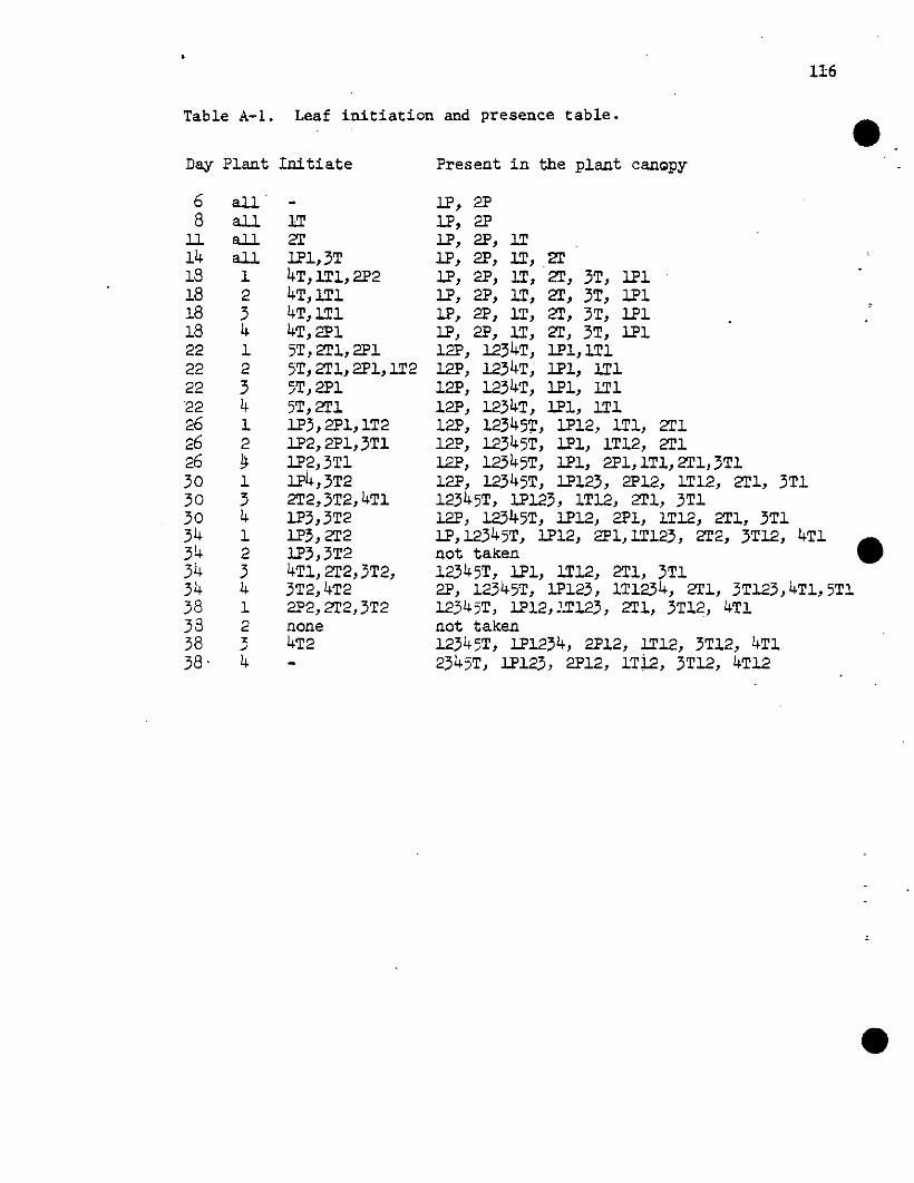
Table A-i. Leaf initiation and presence table.
116
•Day Plant Initiate Present in the plant canQPY
68
II1418181818222222222626263030303434343438333838·
allallallall1234123412!I13412341234
IT2Tl.1?1,3T4T,lT1,2P24T,lT14T,lT14T,2P15T,2T1,2P15T,2T1,2P1,lT25T,2P15T,2Tll.1?3,2P1,lT2l.1?2,2Pl,3Tll.1?2,3Tll.1?4,3T22T2,3T2,4Tll.1?3,3T2l.1?3,2T2l.1?3,3T24Tl,2T2,3T2,3T2,4T22P2, 2T2, 3T2none4T2
l.1?,2Pl.1?,2Pl.1?,2P,lTl.1?,2P,lT,2Tl.1?, 2P, IT, 2T, 3T, l.1?1l.1?, 2P, IT, 2T, 3T, l.1?1l.1?, 2P, IT, 2T, 3T, l.1?1l.1?, 2P, IT, 2T, 3T, l.1?112P, 1234T, l.1?l,lTl12P, 1234T, l.1?1, lTl12P, 1234T, l.1?1, lTl12P, 1234T, l.1?1, ITl12P, 12345');', l.1?12, IT1, 2Tl12P, 12345T, l.1?1, IT12, 2Tl12P, 12345T, l.1?1, 2Pl, IT1, 2Tl, 3Tl12P, 12345T, l.1?123, 2P12, lT12, 2Tl, 3Tl12345T, l.1?123, 1T12, 2Tl, 3Tl12P, 12345T, l.1?12, 2Pl, lT12, 2Tl, 3Tll.1?,12345T, l.1?12, 2P1, lT123, 2T2, 3T12, 4Tl •not taken12345T, l.1?1, lT12, 2Tl, 3Tl2P, 12345T, lPl23, ITl234, 2Tl, 3T123, 4Tl, 5Tl12345T, l.1?12, J.T123, 2Tl, 3T12, 4Tlnot taken12345T, l.1?1234, 2P12, lT12, 3T12, 4Tl2345T, l.1?123, 2P12, ITi.2, 3T12, 4T12
•

•117
APPENDIX B
DETERMINATION OF PHOTOSYNTHETIC PARAMETER VALUES
The photosynthesis submodel of the snap bean model consists of the
equation:
(B-1)
•
In order to obtain values of the parameters a, P RL' and 8n,max'
it is generally necessary to fit eqn (B-1) to data. In the absence of
data, the values will have to be obtained from the literature. In this
appendix, a method for determination of a, Pn,max' RL, and 8 from
published graphs is derived and illustrated •
Determination of a, Pn,max'
In most cases, published data consists of net photosynthesis data.
Thus:,
(B-2)
where Pg is given by eqn (B-1), has to be fited. For all parameters
except 8, obtaining estimates from graphed data is fairly simple since
the initial slope is:
dPn-dI1=0
=a (B-3)
•Pn,max is the upper asymptote, and RL is the intercept on the
Pn axis. Thus a can be estimated by drawing a line tangent to the
curve at the Pn intercept and calculating the slope. Pn,max can
be determined by drawing a line representing the upper asymptote and
reading its value off the Pn axis. Since leaf respiration is

118
assumed to be constant over all light levels, RL is simply the
Pn value at I a O. Frequently data is not available for low light
levels; here the curve may need to be extrapolated to the Pn axis to
obtain the intercept value.
Determination of 6
a. Mathematical Derivation
The calculation of 6 is less simple. Its value determines how
close the curve is to the Blackman limiting response curve:
•
It is possible to derive a method for determination of 6 by considering
P~ " [O'I - RL
Pn max,
for I < (Pn,max+RL)/O'
for I ~ (Pn,max+RL)/O'(B-4)
•the relationship between it and the difference (Q) at the maximum
separation between the two curves.
so that:
Q " PnlI=(Pn,max+RL) / Cl'
(B-5)
= Pn max ,
2(Pn ,max+RL) - J2(Pn ,max+RL)2 - 46(Pn ,max+RL)2= Pn max - -..;;;==-----...;..:=;,..-----..,;;;==--
, 28
2(Pn ,max+RL) - .f4(Pn ,max+RL)2(1-6)
26
= (Pn,max + ~) - (Pn,max
- RL
(B-6)
(B-7)
(B-8)
(B-9) •
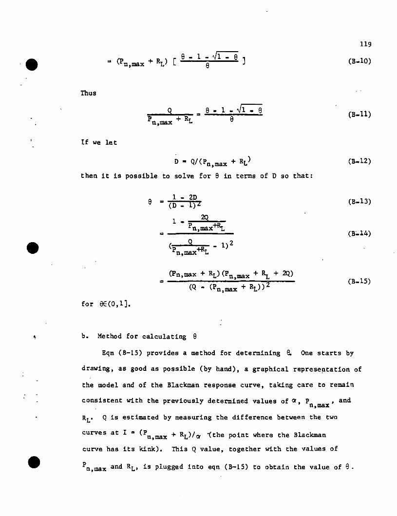
•119
(B.IO)
Thus
If we let
D • Q/(Pn,max + RL)
then it is possible to solve for e in terms of D so that:
(B.11)
(B.12)
•for SE(O,l].
e 1 • 2D= ""'(D';"";;.-1;:;):"'2
2Q1 • ::-..;;;;:",'"":":::'-Pn,max-Hl.r.
=----"--";;;'-
(Pn,max + RL) (Pn,max + ~ + 2Q)
(Q - (Pn max + RL»2,
(B.13)
(B;.14)
(B.15)
•
b. Method for calculating e
Eqn (B-15) provides a method for determining e. One starts by
drawing, as good as possible (by hand), a graphical representation of
the model and of the Blackman response curve, taking care to remain
consistent with the previously determined values of a, P , andn,max
RL• Q is estimated by measuring the difference between the two
curves at I • (P + RL)/- ithe point where the Blackmann,max ....
curve has its kink). This Q value, together with the values of
Pn,max and RL, is plugged into eqn (8-15) to obtain the value of e.
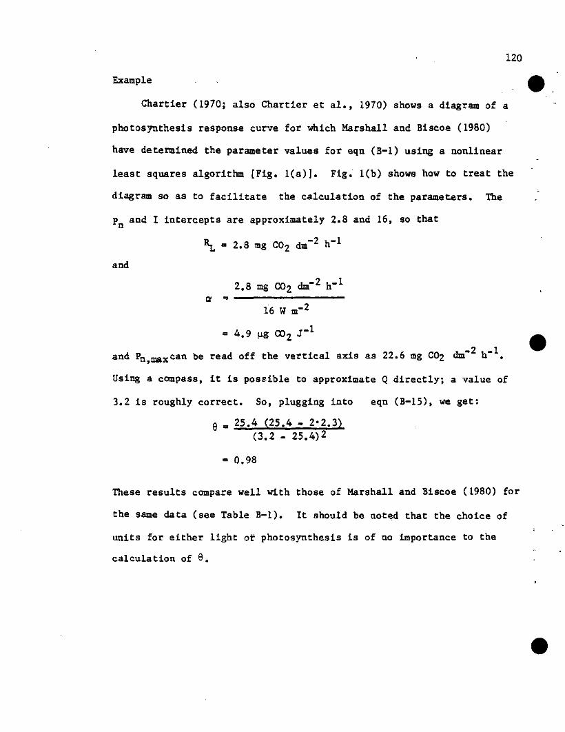
CI =
120
Example
Chartier (1970; also Chartier et al., 1970) shows a diagram of a
photosynthesis response curve for which Marshall and Biscoe (1980)
have determined the parameter values for eqn (B-1) using a nonlinear
least squares algorithm [Fig. l(a) I. Fig. l(b) shows how to treat the
diagram so as to facilitate the calculation of the parameters. The
Pn and I intercepts are approximately 2.8 and 16, so that
~ • 2.8 mg C02 dm-2 h-1
and
2.8 mg CO2 c1m- 2 h- l
16 W m- 2
= 4.9 ~g CD2 r l
and Pn,maxcan be read off the vertical axis as 22.6 mg CO2 c1m-2 b- l •
Using a compass, it is possible to approximate Q directly; a value of
•
•3.2 is roughly correct. So, plugging into
e = 25.4 (25.4 - 2·2.3)(3.2 _ 25.4)2
= 0.98
eqn (B-15), we get:
These results compare well with those of Marshall and Biscoe (1980) for
the same data (see Table B-1). It should be noted that the choice of
units for either light ot photosynthesis is of no importance to the
calculation of e.
•

121
5
• -0--0- c> .0--
20....J:J--
P0"' .....",
/15 9"
""Pa~ (a)10 /
~~
5 l~
~
o~~
0~ 50 100 150 200 250~
I (w m- 2 )
Pa,max ---,-Q ,
20,
• 15
Pa 10 (b)
O+-r--.......--------'"-----..---.,.-50 100 150
I (w m-2 )
200 250
Figure B_1. (a) Net photosynthesis response, Pn (mg CO2 dm- 2 h-l ) forbean plotted against irradiance, t, (symbol 0) redrawnfrom Chartier (1970) with the model [eqn (B_1)] (dashedline). (b) Same as (a) with the Blackman limiting response curve and other guide lines drawn in to allowdetermination of the photosynthetic parameters (see text) •
•

Table B-1. Comparison of parameter values of eqn (B-1) for thedata set of Chartier (1970) determined by the method(see text) and a nonlinear least squares routine.
122
•Nonlinear
Developed LeastParameter Method Squares Units
Ct 4.9 4.9 Ilg CO J-l2
P 2.26 2.27 118 c02
m-2h-ln,max
!1. 0.28 0.23 Ilg c02m-2h-l
e 0.98 0.984 - •
•
•

•
•
•
123
REFERENCES
Chartier, P., 1970. A model of CO2 assimilation. In: Proceedings ofThe LBP/PP Technical Meeting, Trebon, September, 1969, ed. I. Setlik,pp. 307-315. Centre for Agricultural Publishing and Documentation,Wageningen, The Netherlands.
Chartier, P., Chartier, M., and Catsky, J., 1970. Resistances for CO2diffusion and for carboxylation as factors in bean leaf photosynthesis. Photosynthetica 4:48-57.
Marshall, B. and Biscoe, P. V., 1980. A model for C3 leaves describingthe dependence of net photosynthesis on irradiance. I. Derivation.J. Exper. Bot. 31:29-39.
124
APPENDIX CBEAN: PL/I COMPUTER PROGRAM AND NOTES
This appendix contains the listing of the computer program for,
the model BEAN. The job control statements, listed in Table C-1, allow
•the program to run on the IBM 3081 computer. Application may be made on
any machine which supports some form of PL/I. Notes on th~ program are
provided following the source code (Table C-2).
Notes
a. Files
In addition to printing out most of the pertinent information
simulated by the'model, the program also stores information in three
seperate files for further analysis.
are declared
These flies (OUT, OUT2, and OUT3) •
in lines 1250 and 1260 (all line numbers refer to Table C-1
and C-2) and nre identified with specific data sets (BNOUT2, ETAS2, and
CPYOUT, respectively) through the IIG. statements (lines 4550-4565). It
is recommended that these data sets be created interactively prior to
execution of the program. Otherwise different JCL statements
(containing VOLUME, DCB, etc., information) will be required. The exact
syntax of the JCL depends on the machine (see local JCL programmers'
guide) •
b. Compiler
This program was written for the PL/I optimizing compiler, but
should be able to run on any PL/I compiler supporting the "DO WHILE"
syntax. Where this is not available, a simple replacement with an
"IF-THEN-DO" and a "GOTO" statement will make the program conform. The •
only occurrence of this situation would be at line 2040.

•
•
•
125
Table C-l. Job control statements for running BEANon the IBM 3081 computer.
00010 IIBEAN JOB NCS.ES.G7122,LIETH,P=80,T=1 ,M=(2,O),COMPRESS=NO00020 II EXEC PLOCG,00030 II PARM='NA,NX,SMSG'00040 Ilc.SYSIN DD *
Source Program Statements for BEAN model
04540 1*04550 IIG. OOT DD DSN=NCS. ES. G71 22. LIETH. BNOUT2, UNIT=DISK. DISP=OLD04560 IIG.OUT2 DD DSN=NCS.ES.G7122.LIETH.ETAS2,UNIT=DISK,DISP=OLD04565 IIG.OUT3 DD DSN=NCS.ES.G7122.LIETH.CPYOUT,UNIT=DISK,DISP=OLD04570 1*

Table C-2. PL/I comp~ter program of the snap bean model BEAN
00050000600007000080000900010000110001200013000140001500016000170001800019000195002000021000220002300024000250002600027000280002880029000300003100032000330003400035000360003700038000390004000041000420
126
BEAN: PROCEDURE aPrIONS (MAIN);
/ ****************~.............•••••• /~ ~/* SNAP BEAN GRCMTH MODEL *//* THESIS EDITION */~ ~/* BIOMATH PROORAI! PROORAI!MER: *//* NC STA TE UNIVERSITY HEiliER LIETH *//* RALEIGH. NO 27650 SEP. 1982 */~ *// ***•• I ••••••••••* I •••••••• I ••********~~•• ~ •• •••••//* **** /~ THIS IS THE PROGRAl~ OF THE MODEL DEVELOPED *//* IN THE DIS SERTATION OF HElfIRICH LIETH, 1982 • *// *** /
I-I' .1 •• I·W •••• ill •••••••• 1.1 1.1. ' •• 1.1. II ••• II /
/* DECLARATION OF VARIABLES: *// /DCL /* INTEGERS */
(AGE, /* AGE OF LEAF */AGEX, /* AGE OF LEAF, CONVERTED FOR PSIl/ MODEL */CNT. /* COUNTER FOR PAGE SKIP IN OUTPUT */DAY, /* DAY COUNTER */DYFUI, /* FWIIERING DATE */DYPOD, /* POD-FILL DATE */I, /* COUNTER */IO, /* INCIDENT IRRADIANOE AT TOP OF CANOPY */OLD(18). /* AGE OF LEAF */L#. /* LEAF COUNTER */PHI. /* PHOTOPERIOD */ROSTER(18), /* PRESENCEV ABSENCE RECORD OF LEAVES */SNCD(18), /* SENESENCE RECORD OF LEAVES */TOPINDX, /* */TOPLF#. /* INDEX OF LEAF AT TOP OF CANOPY */TOT#L) /* NUMBEIl OF LEAVES IN CANOPY */
FIXED;
•
•
•

•127
Table C-2. Continued•.
•
•
0043000440004500046000470004800049000500005100052000530005400055000560005700058000590006000061000620006300064000650006600067000680006900070000710007200073000740007450075000760007700078000790007950080000810008200083000840008500086000870008800089000900009100092000g-500094')00950009600097000980
DOL /* NONINTEGER */( A. /* CONVERSION llFFICIENCY (I-GROliTII RESP) */
ALPHA, /* QUA!lTUl'I r:FFICIEtICY FOR LIGlIT RESPONSE *;-AREA(IS), /* LEAF AREA OF IlIDIVIDUAL LEAF */ASKL, /* GROSS ASSIlIlLATE AVAILABLE DURING DAY */B, /~ MAINTENANCE RESPIRATIOll */BB, /* LEAF EXPAlISWN PARAMETER ( ) */CIJi, /* COTYLEDON CCNP,{R1HENT (DRY "EIGHT) */GFTOT, /* -TOTLA* .167 FRACTIOll OF CANOPY III FULL 10 */C02FX(18) , /* PHOTOsmTHETIC RATE */CtllILA(18), /* CtllIULATIVE LEAP AREA ABOVE LEAF */CV, /* CONVERSIDrI FACTOR (0 D..... / G GLUCOSE) */DC, /* LOSS OF DRY '.. EIGHT pum COTYL */DP, /* REPRODUCTIVE DRY ... EIGHT INCREMENT */DL, /* LEAP DRY WEIGwr rNCRE2lENT "/ .DR, /* ROOT DRY •.. EIGHT INCREMENT "/OS, /" STE2l DRY "EIGHT INCREMENT "/DT, /* TOTAL DRY '.. EIGHT INCREHENT "/ETAF, /*. • • FRUIT • "/ETAL, /* PARTITION COEFFICIENT POR LEAF CQIIPAR1HENT*/BTAR, /*. • • ROOT • */ETAS, /*.. .. .. STEK .. • /P, /* CtllIULATIVE LEAF AREA '/ARIABLE */FIJi, /* REPRODUCTIVE CQIIPAR1HENT DRY ...EIGHT */GAK, /* COTYLEDON DIf TO GLUCOSE CONVERSION */INITLA, /* INITIAL LEAP AREA */IRR, /* IRRADIANC E */K, /* LIGHT EXTINCTION COEFPICIENT */KK, /* LilAF EXPANSION PARAMETER (GRO"'T11 RATE) "/LOW, /* LEAP COllPARTlU:lIT my ... EIGHT· "/LIGHT(18) , /* IRRADIANCE "/Ml4, /* LEAP EXPASSION PAlL\lIETER (ASSIIlPTOTE) */NA::HL, /* ~IET A3SlNlLATE AVAILABLE DURING DAY "/POO, /" PHO':.JSNTHETIC CONTRIBUTION PRO!! COTYL */PM, /" M'X GROSS PHOTOSiliTHETIC RATE */PIU, /* /lAX NET PHOTOSYIITHETIC RATE "/psm, /* PHOTOSY:/THETIC RATE "/RIM, /* ROOT C<1lPARTlIENT DRY 'iEIGIiT "/RESP, /* DAILY RESPIRATORY COST */RGR , /* R!!lLATIVE GaaiTII RATE OF ·.HOLE PLANT "/RGRC, /* RELATIVE GIIa.T11 RATE OP COTYL CCl4PARTlIEUT */llGRF, /* RELATIVE GIIa.TII RATE 0'1 REPR. C<1lPAR'l'IENT "/RGRL, to RELATH'E GIIa.TII RATE OF LEAF C<1lPARTlIElIT */RGRR. /* RELATIVE GIl OW TIl RATE OP <lOOT C(JIPARTME?IT "/RGIIS, /* RELATIVE GIIa.TIl RATE OP STEM C<1lPAR'J}lENT */ilL, /" LEAP RESPIRATION */RHO, /* CONVERSION PACTOR: LEAP AREA PER G DRY liT */SVo', /* STm C<1lPAR'J}lElIT DRY ·.EIGIIT "/SINK, /* SINK STRElIOTH OP LEAP (NORMALIZED */SNKS(IS), 1* SINK STREGTHS OF LEAVES (U11N0RllALIZED) */TO'. , /* TOTAL DilY 'igIGHT */TIIETA, /* psm 1I0DEL PARAMETER */TO'CLA, /* TOTAL LEAP AREA OF PLANT */TOTSNK, !" TUTAL OF SNKS(*) */TO'N, /* TOTAL NET PHOTOSmTIIATS PRODUCED */lI( 18), ;* PIlOTOSTIfTHATE PRODUCED BY LEAP PER DAY */x/fX) /* TE;UQRARY '/ARL\BLE */
DECIlIAL FLOAT;

Table C-2. Continued.
128
•
CHAR(loo);DCL LFID(18) CHAR(3) IliiTIAL ('IP ','2P ','IT ','2T ','3T ','1Pl',
'1T1','4T ','2P",'5T ·,'1T2','2T1',t 1P2' t t;T 1 I , '1 P3' 1'1 T3' , '4Tl I , • ;T2');
/* LINE OF ASTERlXES FOR BOXING OUTPUT/* LINE OF SPACES BE:'l'WEEN NO ASTERIXES (")
/•••••• I.***.......»*~**......//* LEAF INITIATION IUTRIX: *//* COL I: DAY OF IliITIATION *//* COL 2: HEIGHT RANKING *//* FROM TOP. *// //* INDEXING IS CHRONOLOGICAL *//............*~*............**-:t**/
DeL /* NONINTEGER */GAMMA(18.2) BINARY FIXED
•*/*/
/* lP *//* 2P */
. /* 1T *//* 2T *//* 3T *//* lPl *//* lTI *//* 4T *//* 2Pl *//* 5T *//* lT2 *//* 2TI *//* lP2 *//* 3Tl *//* lP3 *//* lT3 *//* 4Tl *//* 3T2 */
18,17,16..13,11 ,15,12.8,
14,5.
10,7.6.9,1•2.3.4);
INITIAL (3.3,
10,13,15.16,17,18.20.22,24,25.26.28.30,31,32,34.
OUTPUT STREAM;DCL /* FILES */
(OUT. OUT2, OOT3)
DC L /* CHARACTER */(BOXI ,BOX2)
0099001000010100102001030010400105001060010700100001090011000111001120011300114001150011600117001100011900120001210012200123001240012500126001270
•

129
Table C.2. Continued •
f* DAY *//* FLOWERING INITIA TrOll DAY *//* POD FILL INITIATION flAY *//* MICRO. EINSTEIN /OI"M"SEC) * //* GRAI'[ GLUCOSE *//* H"M *//* SEC / DAY */
/* - */ .f* GRAM !JII / (GRAM !JII * DAY) */f* H"M LEAF AREA / GR.~ !JII *//* - *//* GRAI'[ GLUCOSE!(GRAl4 Ili * DAY) *//* GRAIl D.... / GRAI'[ GLUC OSE "/
/* GRAIl Ili * //* GRAM Ili */f* GRAM !JII *//* GRAM !JII *//* GRAM !JII *//* GRAM !JII *//* H"l! *//* M"M *//* M"M */
BOI2-'·,DAY-5;DYFUl-24;DYI'OD-27,I0-590;TOiV-<l;INITLA-. 0005;PHI-32400;TOT"l.-2 ;TOPINDX-18,DO I-I TO TOPINDX;
CUllLA(I)-O;ROSTER(I )·0;AREA( I )-0;SNCD(I )., ;
END;ROSTER(GAMMA(l ,2»-1;ROSTER(GAMMA(Z,2»-Z;TOPLF#-GAIlMA( 2,2);THETA-.9435;GAIl-. ee;iUlo-.0563;A-·75;B-. 0225*.682;CV-l .0;MM-as. 7785;BB-ZO. 9818;KI-3. 60308E-3;CIli-.04;LW-.0347;SIlW-.024Z;RIlW-.0204;FIW-o.O;TDW-LD'i+SW+RIli +FIli+CIli;AREA(l )-.0010 ;AREA(Z)-.OOlO;TOTLA-AREA(l )+AREA(Z);
/ //* IIIITIALIZATION OF YARIABlES . */;.~ *••* * **.A ••• ~»~ /
BOX1· 1 ••• IfI ••••••••-)., , ' ~~
................................................... ' .,,"II*' .,
0128001290013000131001320013300134001350013600137001380013900140001410014200143001440014500146001470014800149001500015100152001530015400155001560015700158001590016000161001620016300164001650016600167001680016900170001710
..•
•
•

130
Table C-2. Continued. e.01720017300174001750017600177001780017900180001810018200183001840018500186001870018800189001900019100191501920019300194001950019600197001980019900200002010020200203002040020500206002070020800209002100021100212002130
/ I~.*** *.~»**I •••••• I* /f'O OUTPUT INITIAL CONDITION 'Of/*..*********..**••••••********** ********••***** /
PUT SKI P EDIT (BOX1) ( A( 100) ) ;PUT SKIP EDIT (B0X2)(A(l00»;PUT SKIP EDIT (' 'O' ,'INITIAL CONDITIONS',' 'O' )(A(l) ,COL(41) ,A(l8),
COL(100),A(1 »; .PUT SKI P EDIT (BOX2)( A( 100) );PUT SKIP EDIT ('.' ,'DAY' ,'LEAF D1i' ,'STm !JII' ,'ROOT D1i' ,'FRUIT !JII',
'TOTAL 0',' ,'COTYL. !JII ','TOTAL LA' ,'.' )(A(l ),X(2), .A( 3) ,3(X (6) ,A( 7) ) , 2(X (5 ) ,A(8) ) ,X(4 ) ,A( 10) ,X(4) ,A(8) ,X(2 ) ,A( 1 »;
PUT SKIP EDIT(''''', 'GRAMS', 'GRAMS', 'GRAMS', tORAMS', 'GRAMS', 'GRAMS','SQUARE' ,'·')(A(l ),X(4),6(X(8),A(5» ,X(7),A(6),X(3),A(1 »;
PUT SKIP EDIT('·',' ','METERS' ,'·')(A(l ),X(76),A(7),X(6),A(6),X(3),A(1 ));
PUT SKI P EDIT ('.', DA Y, LOll , S!JII , R!JII , FIlIi , TDIi , C!JII , TOTLA, ' .' )(A(l ),X(2),F(2),X(1 ),7(X( 4),E(9,2»,X(2),A(1 »;
PUT SKIP EDIT (B0X2)(A(100»;PUT SKIP EDIT (BOXl )(A(100»;CNTa 10;
/, *** *** 11 /
f'O 'Off'O START OF GRCMTII MODEL 'Of/ **** ,••••.• 1/
NXTDAY: DAY-DAY+l;
/.* *** ******~** ********* //*** INITIATE NE'I LEAVES ** // *******************••; *** ****/
IF TOT#L<TOPlNDX THENDO i'HILE(GAMMA( TOT#L+l ,1) - DAY);
TOTLAaTOTLA+INITLA;TOT#'L-TOT#L+l ;AREA(TOT#L)-INITLA;I-G~~(TOT#L,2) ;ROSTER(I)-TOT#L;IF I<TOPLF# THEN TOPLF#-oI;IF TOT#L>aTOPlNDX THEN GaTO NXTLN;END;
•
•
"
131
Table C-2. Continued.'.
•
"
•
021400215002160021700210002190022000221002220022300224002250022600227002200022900230002310023200233002340023500236002370023000239002400024100242002430024400245002460024700240002490025000251002520025300254002550025600257002580025900260002610026200263002640026500266002670
"
RXTLN:/ - /1* CALCULATE THE EXTIl1CTION COEF?ICIENT '*1/ ****••» I ~ /
K-7.63 + 2. 23/'roTLA;
/ 11_//* CALCULATE THE CU14ULATIVE LEAF AREA DISTRIB. FRG'I THE TOP DOliN *1~ , /X!fX-o;DO I-TOPLF# TO TOPIlIDX;IF ROSTER(I »0 THEIl DO;CUMU(I)-X/fX;xf/X-x/f1. + AREA( ROSTER(!));ERD;
ERD;
/ ~*••••••••• ............//* CALCULATE THE PHOTOSYNTHETIC CONTRIBUTION FRCX'I THE COTYLEDON *1I*••••••••••••II ••••• I! ~ /
AGEX-DAY;IRR-IO;
IF AGEX <- 14 THEIl ALFllA--. 6173+. 2811*AGEX - .000093*AGEX*AGEX;ELSE ALFllA--. 1641 *( AGEX-1 4.81) + 1. 464;
IF ALFllA<O THEIl ALFllA=O;IF AGEX <- 10 THEN FM-218.9*(AGEX-l0.51)+1089;
ELSE PM- 214.1+ 166.S*AGEX - 7. 921*AGEX*AGEX;IF F!l<0 THEIl F!l-o;IF AGEX < 10 THEN RLa 1962 -333.7*AGEX +15.77*AGEX*AGEX;
ELSE R101 97.7;IF RL>400 -THEIl R10400;PMX-P[4+RL;X/fX-ALPHA*IRR + P~X;
PSYN- (X/I1. - SQIlT(X/f1.*X!fX - 4*ALPHA*PKX"THETA*IRR))/(2"THETA);PDC - .682*PSlll*.OOO3*PHI*1.0E-6; I*ASSUME SURFACE AREA-, SQ CM *i
;- /1* DETEIlIlINE THE VAWES FOR THE INDIVIDUAL LEAF VARUBLES */, *** ,
TOTSNK-D;TO'lW-o;DO L661 TO TOT#L;IF SllC D(L# )-0 THEIl CO'ro BPI;
AGE-DAY-GAMKA(L#.l );OLD(L#)-AGE ;
FoCUlIU( GA!'llIA( L#. 2»);CFTOT"'rOTU* • I 67;IF DAY < 14 TH~1 IRR-IO;
ELSE IF F<CF'roT THElI IRR-IO;ELSE IRR-IO*EXP(-K*F);
LIGHT(L#)-IRR;

132
Table C-2. Continued. ••02680026900270002710027200273002740027500276002770027800279002800028100282002830028400285002860028700287502880028900290002910029200293002940029500296002970029030029900,000030100302003030030400;050030600;070030800;0900310003110031200;13003140031500;160031700;1800;190
/•••*~••~ *** ~••••* »».~.***..*..** **//* CALCULATE THE PHOTOSYNTIlElTIC PARAME:TERS */,..******it-:t :t f »***'.**H***·••H ******· .jo. H,:t**·::t:t J"» »* /AGEX~(AGE+5)*2/3; /* COlIVERSION 'ro Cor~PtlNSATE FOR THE· FACT THAT */
/* A DIFFE:llENT CUL'rIVAR WAS USED TO DEVELOPE THIS MODE:L *//* AND LEAF INITIATION .~ TIME OF SOWING . */
IF AGEX <~ 14 THEN ALPHA~-.6173+.2811*AGEX - .OO9493*AGEX*AGEX:ELSE ALPIlA--.1641*(AGEX-14.81) + 1.464:
IF ALPHA<O THEN ALPHA-O;IF AGEX <~ 10 THEN PM-218. 9*(AGEX-l0. 51 )+1089;
ELSE PM~ 214.1+ 166.5*AGEX - 7.921*AGEX*AGEX:!1 PM<O THEN PMaQ;IF AGEX < 10 THEN RL~ 1962 -333.7*AGEX +15.77*AGEX*AGEX;
ELSE RL-1 97.7:IF RL>400 THEN RL-400;
/"*****".*****.'~».*.**"I"'******.****"."••»•••••*.***.*....,//* GROSS PHOTOSYNTHESIS RATE *//****......***.**..***********~.**.*•••~.~.***..*••••••••****.*»**/PMX~PM+RL:
PU-PMX*1.14:XUX-ALPHA*IRR + PMX;psm~ (xlIX - SQRT(XIIX*XUX - 4*ALPIlA*PMX*THETA*IRR))/(2*THElTA):C02FX(L#)-PSYlI ;/~'******"'••"*****"I"'******.********•••••"""I***""*//* TOTAL AMOU!l·r OF GRQl;S PHOTOSYNTHATE * //.****~**~** ~~~.».* **** *** ** *** *•••••*.*/
1i(L#)- • 682*psm*AilEA( L,j!)*PHI*1 •OE-6;
/ *****.*** ·:t.:t·••· ·•· 'lt:l* /
/* DROP LEAVES OPERATING BELOW Til;;: COMPENSATION i'OIN'r *//************** **~*.~••~ ** * **/IF P'.:lTN<O a AGE>15 THEIl DO;
SNCD(L#)-O:W(L#)~O:
END;
/ ****.**.***.*:t:t:t~ ***** **..**•••*******••*****.//* TOTAL AMOUNT OF GROSS PIlOTOSYNTHATB *//..*****...**.*...**...*......* ••~.:t:t•••••*...***.........*******/
/*..+*******.....*••*.**•••• ~••••*...*~....***.**...**•••***.*.//* CALCULATE SLVK STRENGTHS (UNNORMALIZED) *//**.....**...*...**********.**••~»••••*.......*..*******.*.******/SNKS(L#) • ~~/(1+BB*EXP(-MM*KK*(AGE+l )))
-MI'I/ ( 1+6B*EXP (-,iM*KK*AGE))IF SNCD(L#)-O THEN SNKS(L#)-O;TOTS~~-TOTSNK+SNKS(L#);
SP1: END;
•
•
133
Table C-2. Continued•
IF DAY<DYFUl THEN DO;ETAL-.5; ETAF-.OO;END;
ELSE DO;ETAL--(DAY-42)/36; ETAF-.5-ETAL; EllD;
IF ETAL<O THEN DO;ETALoQ; ETAF-. 5; EllD;
••
•
•
03200032100322003230032400325003260032700328003290033000331003320033300334003350033600337003380033900340003410034200343003440034500346003470034800349003500035100352003530035400355003560035700358003590036000361003620036300364003650036600367003680
~"""""""""""'I"""""""""""""'"•••••••••••• /I- DETERMINE PARTITION COEFFICIENTS ·1/*...................................................... */
I- -I·I· -II- ETAL AND ETAF - 1I- ARE AFFEX:TED BY -If> THE FLOWERIllG -II- DATE -If> -II- -If> -II- -II- -I
IF DAY<DYPOD THEN DO; ,. -IETAS-.32-(DAY-l )/26; ETAR-.5-ETAS; I- ETAS AND ETAR ARE -IEND; I- AFFEX:TED BY THE -I
ELSE DO I- POD FILL DA TE -IETAS-. 32; ETAR-. 18; END; f> -I
IF ETAS<O THEN DO; ,. -IETASaO; ETAR-.5; I- -I&RD; / ;
PUT FILE(OUT2) SKIP EDIT (DAY, <:rAL, ETAS, <:rAR, ETAF)( F(2) ,7(X(2) ,F(7 ,4»);
/ /,. CHECK THAT THE: ETA'S ADD lIP TO 1 -I/ ..11, , ••••••••••••• /
XUX-ETAL+ETAS+ETAR+ETAF;IF Xi/X<.99 : XUX>I.01 THEN PUT LIST .
('ERROR: ETA"S DONT ADD lIP TO ONE. SlIM-' ,XUX);
I·······w ......................•....................................../I- GROWTH A!/D MAIllTENACE RESPIRATION -I/................................. */
DC - GAM-CIlo'; I- G IlIlY !lATTER FRQIl COTYL. -/ASHL-TOTW+DC/CV +PDC; /- TOTAL ASSIMILATE (G GLUCOSE) -/XUX- B"TDii; I- <-- MAIllTENACE RESPIRATION ./IF XUX>ASML THEN NASML-O; /- -;
ELSE IIASoiL-ASML-XUX; /- - iNASlU..'A-NASllL; I- DEDUCTON FOR GROWTH RESPIRATION -/RESP-ASML-NASML; /•••••••••••• , /
I········· ··•···· ..•··········..······ ..•······ //- CALCULATE IllY EIGHT INCRE1H::ITS -// /
DT"'NAS/'lL-CV;DL-ETAl."DT; DS-ETAS"DT; DR-ETAR"DT; DF-ET~DT;

134
Table C-Z. Continued.
036900370003710037200373003740037500376003770037800379003800038100382003830038400385003860038700388003890039000391003920039300394003950039600397003980039900400004010040200403004040040500406004070040800409004100041100412004130041400415004160·0417004180041900420004210042200422504230
/ *** ** •••• t/. MODIFY DRY WEIGHT OF EACH CCfoIPAR'nH:NT. CALCULATE: REL. GRCI.TH RA1'E*//** **.*••********~******••***********.**************.********/
LDlioLDW+DL; IF :.IlW>O THEN RGRIrDL/LDW; ELSE RGRIrO;SD'o'oSU.+DS; IF SD'o'>O THEN RGRS'DS/SD'o'; ELSE RGRS=O;RD'o"RDII+DR; IF RD'o'>O THEN RGRR'DR/RDII; ELSE RGRR=O;FD'o'-FD'o'+DF; IF FU.>O THEN RGRF-DF/FI/o': ELSE RGRF=O;CD'o'-e I/o' -<;AM· CI/o' ;IF CI/o'>O THEN RGRC--GA!l; ELSE RGR=O;TDW-LDW+SD'o'+RD'o'+FD'o'+CD'o';IF Tlli>O THE:lI RGR-DT/TIY.; EISE RGR=O:
/ 1//. !lODIFY LEAF AREAS BASED ON LEAF MATTER ALLOCATION (DL) AND .//* llORllALIZ ED SINK STRENGTHS. */,.********.***** /
TOTLA=O;DO L# ° 1 TO '!'OT#L:/ **** **** II/* NORllALIZ E SINK STRENGTHS *//** *** ** 1 * /SINKoSNKS(L#)/TOTSNK:SNKS(L#)oSINK:/*•••••••••**** **//* CALCULA TE /lEl{ LEAF AREA OF LEAF 1# *// ••• ~ ••••••• I I *•••••••••• /AREA(L#) g AREA(L#)*SNCD(L#) + SINK*RHO*DL;TOTLA-TOTLA + AREA( L#);END;
j** ******* ****•••,•••••••• m1 ***.*//* PRIllT OtJr DA ILY RESULTS *//.*** ** ****/
PUT FILE(OUT) SKIP EDIT (DAY.LDW.SD'o'.Rtw.FD'o'.RGRL.RGRS.RGRR.RGRF.RG!'. NASi'lL. RESP)( F( 2).11 (X (1 ) •E(9 .2»);
PUT SKIP EDIT (BOX2)( A( 100»;PUT SKIP EDIT(··· .·DAY - •• DAY.
'LEAF' •• COTYL' •• STili' •• ROOT' •• Rm •••• TOTAL' •• *') (A( 1 ). X(3) •A( 6) •F( 2) •X( 1, ) .A( 4) •X(9 ) •A( 5 ) .X(9) .2 (A( 4) .X(9 ) ) •A( 5) •X(9 ) •A( 5 ) •COL(100).A(' »:
PUT SKIP EDIT (B0X2)(A(100»;PUT SKIP EDIT('*' .·DRY ilEIGHT' .LDW.Ctw.S17•• RD'o'.FD'o'.TD'o'.·.·)
(A( 1) .X(3 r.M 12) .6(X( 4). E(9. 2» .COL(100) .A(' »;PUT SKIP EDIT (BOX2)(A('OO»:PUT SKI P EDIT(··· • 'IllCREME:lIT '. DL. IX:. til. DR. DF. Dr•••• )
(A(1 ).X(3).A(12),6(X( 4).E(9.2».COL(100).A(1 »;PUT SKIP EDIT (B0X2)(A(100»;PUT SKIP EDIT(··· .' RGR •• RGRL. RGRC. RGRS. RGRR. RGRF. RGR.· *')
(A( 1 ),X(3) .A( 12) .6(X( 4). E(9. 2» .COL(' 00) .A( 1»;PUT SKIP EDIT (BOX2)( A('OO»:PUT SKIP EDIT(··' " PART. COEF', ErAL, . -' I ETAS, El'AR, ETAF, '1 .0000· , I.' )
(A( 1 ) .X(3) •A( 12) .X(5 ) .F( 6 • 4) .X(10) .A( 1 ) •X(2 ) •3(X(7).F(8.4) .X(7).A(6).COL(100).A(1 »;
PUT SKIP EDIT (BOX2)( A( 100»;CNT"CNT+11 :
•
•
•

135
Table C-2. Continued ••
•
•
042400425004260042000429)04300043100432004330043400435004360043700438004390044000441004420044300444004444044450444604450044600447004400044S504490045100451404516045180451904520045250453004535
/ ...,.••" **.».:;.*.»10 /;» FRmT CUT CANOPY F~OFILE .;,......***~*.~ ******** lt**** » *••lt.»•••* /
PUT SKIP EDIT ('.' • 'CANOPY PROFILE: ' • •• ' )( 1.( I ) .X(3) •A( 15), COL( I00).A( 1 )) ;
PUT SKI P EDIT (BOX2)( A( 100) ) ,PUT SKIP EDIT C'.'.' ID'.' AGE'.' AREA'. 'LIGHT', ·PSYN·. 'PHSYNTHATE'.
'SINK' • ••' )( A( 1) .X(8) .A(2) ,X(8) .A(3) .X(9) .A(4) .X(8), A(5) .X(11 ),A(4) .X(7) .A( 10) .X(7) .A(4) .COL( 1(0) .A( 1 )),
PUT SKIP EDIT('·· .. DAYS' .' SQUARE' ,'llICROEINST' ,'rUCRO G' " G GLUCOSE'.••• )( A( 1) .X(17) .A(4) .X(8) .A(6) .X(5) .A( 10) .X(7) .A(7) ,X(7) .A(6).COL(loo).A(1 )),
PUT SKIP EDIT(··'.·r~Ell'ERS'.'/(I~Il"SEC)'.·C02·.'PERDU·.··')(A( 1 ) •x(29) •A( 6) •X(5 ) •A( 10) •X(9 ) •A( 4 ) •X(8 ) •A( 7) •COL (100) •A( 1 )) ,
DO L#- 1 TO TOPINDX;I -ROSTER(L#);IF ROSTER(L#»O THEN DO;
PUT SKIP EDIT(··' .LFID(I).OLD(I).AREA(I),LIGHT(I),C02FX(I),W(I).SNKS(I) • ••• )( A( 1 ) .X(8) .A(3) .X(S) .F(2) .X(8), F(6. 4) .X(8) .F(3).X(8) .F(9. 2) .X(7).F(7, 4) .X(7) .F(6. 3) .COL(loo) .A( 1 ));
PUT FILE(OUT3) SKIP EDIT (DAY.I.OLD(I).LFID(I).AREA(I).LIGHT(I)•C02FX(I) •W( I) •SNKS(I) •SNCD( I)).(3 (x (2 ) •F( 2 )) •X(2 ) •A(3 ), 5(X (2 ) •E(9. 2)) •X(2 ) •F( 1 )) ,
END;END;PUT SKIP EDIT (BOX2)( A( 100 ).);PUT SKIP EDIT (BOXI )(A(loo)),CNT-CNT+7+TOT#L ,
IF DAY < 45 THEN DO;IF (60-CNT)<-(TOT#L+19) THEN DO,
PUT PAGE,PUT SKIP EDIT (BOXI)( A( 100)),em-t;
END;GOTO NXTDAY,
END,END; /. TERIl INA TE PHOGRAI! • /

136
Each panel, (except for the initial one) contains a canopy profile ~
of the plant with summaries for each leaf. The leaves are ordered as
they would be in the canopy (third lateral trifoliates at the top;
primary leaves at the bottom). The canopy.characteristics listed are:
leaf age, leaf area (m2), available photosynthetically active
radiation (~·Einstein m-2 s-I), photosynthetic rate (mg CO 2 .
-2 -1)m s , total amount of photosynthate produced
(g CH20 day-I) and the sink strengths (no units) of each leaf.
c. Output
The output consists of daily summaries of plant and canopy
characteristics. Table C-3 shows the first page of output from BEAN
(Table C-2); the first frame contains the initial conditions, the second ~
frame cont3ins information from day 6. (It should be noted that the
notation 3.47E-02 means 3.47.10-2). Table C-4 contains the output
for day 38.
~

• , , , • ", •
Table C-3. Sample Output of BEAN (days 5 and 6) •
....................................................................................................• •• INITIAL CONDITIONS •• •• DAY LEAF 1M ST!2I 1M ROOT 1M FRUIT 1M TOTAL DW COTYL. 1M TOTAL LA •• GRAMS GRAMS GRAMS GRAMS GRAMS GRAMS SQUARE·
• METERS •• 5 }.47E-Q2 2. 42E-Q2 2.04E-Q2 O.ooE~ 1.19E-Ql 4.ooE-Q2 2.ooE-Q}·• •••••••••••••••••••••••••••••••••••••••••••••••••••••••••••••••••••••••••••••••••••••••••••••••••••••• •• DAY· 6 LEAF COTYL ST!2I ROOT REPR. TOTA L •• •• DRY WEIGHT 4.10E-Q2 }.68E-Q2 2. SOE-Q2 2.59E-Q2 O.ooE~ 1.29E-Ql ,.• •• INCR!2ImT 6. }2E-Q} }.20E-Q} 7. 71E-Q4 5· 54E-Q} O.ooE~ 1.25E-Q2 •• •• RGR 1. 54E-Ql -8.ooE-Q2 }.11E-Q2 2.14E-Ql O.ooE~ 9.81 E-Q2 •• •• PART. COEl' 0.5000 - 0.ai15 0.4385 0.0000 1.0000 •• •• CANOPY PROFILE, •• •• ID AGE AREA LIGHT PSYN PHSYNTHATE SINK •• DI.YS SQUARE MICROEINST MICRO G G GLUC •• METERS I( M"II"SEC) CO2 PER DAY •• 2P 3 0.0012 590 294.62 0.0065 0.500 •• lP 3 0.0012 590 294.62 0.0065 0.500 •• •....................................................................................................
....."""

Table C-4 • Sample Output of BEAN (day 38).
••***.********•••***•••**********»••***••" ............................-•••••••••••••••••»••••••••••• •• DAY • 38 LEAF COTYL STEM ROOT REPR. TOTAL •" •• DRY WEIGHT 2. 32E tOo 2.55E-03 2.04EiQO 1• 47Ei{)Q 1. 19Ei{)Q 7.03EiQO •• •• lliCUErl EilT 5.04E-02 2. 22E-04 1.45E-ol 8. 17E-02 1.76E-ol 4. 54E-ol •" •" RCR 2.18E-02 -8.00E-02 7.10E-02 5.55E-02 1.'48E-ol 6. 46E-02 •" •" PART. COEl' 0.1111 - 0.3200 0.1800 0·3889 1.0000 •" •" CAliOPY PROFILE: •• •" ID AGE AREA LIGHT PSYH PHSYliTHATE SINK "" DAYS SQUARE MICROEINS'£ MICRO 0 o OLUC "• METERS I( M"M"SEC) CO2 PER DAY •" lP3 8 0.0036 590 559.78 0.0399 0.136 •" 1T3 7 0.0029 590 559.78 0.0319 0.126 "" 4Tl 6 0.0023 590 483016 0.0216 0.112 •• 3T2 4 0.0014 590 384.64 0.0102 0.Cf18 •• 5T 16 0.0091 590 796. Cf1 0.1584 0.049 "" lP2 12 0.0067 590 739.77 0.1039 0.112 "" 2TI 13 0.0074 328 444.44 O. G/OO 0.096 •• 4T 20 0.0103 276 342.75 O. G/80 0.016 •" )'£1 10 0.0051 216 264.62 0.0277 0.136 •" lT2 14 0.0081 192 263.90 0.0457 0.Cf19 " "
" 3T 23 0.0106 159 148.32 0.0346 0.006 ".' ITI 21 0.0105 124 135.36 0.0312 0.012 •• 2T 25 0.0106 96 58.50 0.0137 . 0.003 "" 2Pl 18 0.0099 74 106.06 0.0230 0.028 •" lPl 22 0.0106 59 55.05 0.0128 0.009 •• IT 28 0.0106 46 12.91 0.0030 0.001 "• 2P 35 0.0093 35 0.00 .0.0000 0.000 •" lP 35 0.0093 28 0.00 0.0000 0.000 " f-'• " W•••••••••••••••••••••**••»••»......................**............................................... 00
• " •• ., . v~.......... ,
.' . .