Light Stop Notes

by Flip Tanedo

Abstract

These are notes on light stops. Usually I hand write these notes, but since there are multiple

references it’s easier to keep track of them in a single document.

1 Motivation

We would like to explore the phenomenology of models with light stops. Why?

1. Experimental constraints on degenerate squarks. Assuming degenerate squarks(e.g.invoking flavor-universal soft terms to avoid flavor-changing neutral current bounds)leads to a squark mass scale of over 1 TeV (in fact, maybe more like 1.5 TeV; see 1102.5290).[Image: see H. Bachacou talk at Lepton-Photon ’11.] However, if we only assume flavoruniversality in the first two generations, we can still avoid FCNC bounds while

2. Natural SUSY. The third generation is special. It’s the stop loop that cancels the toploop that is the dominant contribution to the quadratic cutoff-dependence of the Higgs mass.As discussed below, there are only a few sparticles which you really need to be accessibleat the early LHC, and the stop is the only (and most important) squark on this list.

3. Little Hierarchy problem. This is again saying the same thing slightly differently: naiveapplication of experimental bounds suggest that the SUSY scale must be above the 1 TeVscale; if this is so, then why is the Higgs mass below the TeV scale? As explained above,the point is that while the rest of the SUSY spectrum may be heavy, a light stop canaccommodate a light-ish Higgs without too much tuning. The stop is special: it has O(1)couplings to the Higgs (Yukawa) as well as strong couplings to the color sector.

• 1% tuning implies stops below 1 TeV. Other sfermions can be five times heavierwithout costing any fine-tuning.

4. Light stops can be generated from RG running alone. See Stephen Martin. This isdue to the negative contribution to the running coming from the Yukawa interaction.

• e.g. light stops through gauge mediation. Usually we say gauge mediation is flavorblind, but recall Yael’s seminar talk 1103.0292, can use messenger–matter couplingsto give flavor-dependence. General gauge mediation gives a tool for considering astop NLSP (gravitino LSP since this is a low scale mediation).

5. EW-scale baryogenesis. The matter–antimatter asymmetry (“baryon asymmetry of theunvierse”) can be explained through the CP phases in the MSSM that aren’t in the SM.Requires baryon number violating processes to be out of equilibrium at nucleation tem-perature, which in turn requires the (sphaleron energy/critical temp) to be smaller thanthe expansion rate of the universe. The leading contribution to this ratio depends on thecoupligns of light bosons to the Higgs. 0809.3760.

• Cultural note: EW baryogenesis is one popular option for the baryon asymmetry.Others include leptogenesis and Affleck-Dine.

• However, DC et al. seem to have done a lot to exclude this story: 1203.2932. (Seetheir intro for references and reviews.) Since the Higgs is 125 GeV, EW baryogenesisin the MSSM would require (as per the Chicago analysis) a TeV scale left-handedstop and a 100 GeV right-handed stop. [By the way, DC continues to use italics toemphasize sentences in his papers.]

6. Interesting phenomenology that is different form other squark searches.

Other ways out:

• Some other protection mechanism is operative at the TeV scale and SUSY may live at the10 TeV scale. e.g. “Schlittle Higgs” (SUSY little Higgs).

1

• 125 GeV “Higgs” is actually a (techni-)dilaton.

2 Effective\Natural\Minimal SUSY

The main idea is to consider the ‘minimal’ SUSY spectrum that should be accessible to the earlyLHC in order to solve the Hierarchy problem. The main ingredients are:

• Light third generation squarks (light-ish stops) at a few hundered GeV. These run in theHiggs loop and cancel the third generation Standard Model fermion loops.

• A not-too-heavy gluino (less than a couple of TeV) since these contribute to the Higgs massat two-loop level. Note that the gluino tends to want to pull the stop mass up due to itslarge RG coefficient.

• Once you set the gluino mass, unification fixes the electroweak-ino masses to be in the fewhundred GeV range (since the spectrum is given by the ratio of gauge couplings).

• The Higgsinos are also in the same light-ish ballpark since they get their masses from theµ term, the same source as the Higgses. What about soft breaking terms? You can’t writeany by symmetries.

2.1 Main References

• Papucci, Ruderman, Weiler, 1110.6926. Natural SUSY Endures.

• Brust, Katz, Lawrence, Sundrum, 1110.6670. SUSY, the 3rd Gen, and the LHC.

• Kats, Meade, Reece, Shih, 1110.6444. The Status of GMSB After 1/fb at the LHC.

• Older papers with the same basic ideas:

◦ 1007.3897. Effective SUSY at the LHC

◦ hep-ph/9607394. The More Minimal Supersymmetric SM. (Cohen, Kaplan, Nelson),seems to be the original reference.

2.2 Review: Higgs in the MSSM

∆mh2(stops) =

3

4π2cos2αyt

2mt2ln

(

mt1mt2

mt2

)

. (smallmixingα)

Alternate derivation: integrate out stops completely and check their contribution to the Higgsquartic interaction. In the decoupling limit mA0≫mZ, then the Higgs mass can saturate bounds:

mh2 = mZ

2 cos22β+(loops).

Including the effect of stop mixing, we have

mh2 = mZ

2 cos22β+3

4π2sin2βyt

2

mt2ln

(

mt1mt2

mt2

)

+ct2st

2(

mt22 −mt1

2)

ln

(

mt2

mt12

)

+3

4π2sin2βyt

ct2st

2

mt2

(

mt22 −mt1

2)

2− 1

2

(

mt24 −mt1

4)

ln

(

mt2

mt12

)

Note that since yt∼mt, the prefactor yt2mt

2∼mt4, which is usually how this dependence is written.

2.2.1 Comments on the calculation, effective potential method

It may be helpful to understand the origin of the terms above. From the Sparticles book (section10.6) we note that there are three ways to calculate these corrections.

1. Direct calculation from diagrams

2 Section 2

2. Use the RG flow from the SUSY scale down to to the weak scale. See hep-ph/9308335.

3. Effective potential.

The effective potential method is not as numerically accurate, but is pedagogically more clear. Theloop level effective potential is

V(1)

(Q) = V (0)(Q)+1

64π2STrM4(h)

[

lnM2(h)

Q2− 3

2

]

.

Here V (0) is the tree level potential with renormalized couplings at the scale Q. Note that thesupertrace vanishes in the supersymmetric limit, so as expected the potential is protected by SUSYand is corrected only to the extent to which SUSY is broken. The factor of 3/2 is a relic of MSrenormalization, see Peskin (11.78); e.g. it is associated with the freedom to add a finite counterterm that is a quartic polynomial in h (see Hugh Osborn’s AQFT notes).

We now focus on the contributions from the stops to the Higgs potential. In the absence ofstop mixing (which we address below) and assuming equal soft masses m for the stops, we havethe following field-dependent masses:

mt2(h) = yt

2|hu|2mt

2 = m2 + yt2|hu|2 ,

where we drop O(gEW2 ) contributions from D-terms. The point now is to consider the contributions

to the supertrace, remembering the weighting by the degree of freedom for a particle of a givenspin. The top is a Dirac fermion with four degrees of freedom, each stop is a complex scalar withtwo degrees of freedom each. There is also a color factor of three. The loop-level correction is thus

∆V (1) =3

16π2

[

mt4

(

lnmt

2

Q2− 3

2

)

−mt4

(

lnmt

2

Q2− 3

2

)]

.

The next step is to minimize the loop corrected potential. Since ∆V (1) only involves hu, the tree-level constraints on mHd

are unchanged (see the Appendix):

mHd

2 + |µ|2− b tan β+mZ

2

2cos 2b = 0.

On the other hand, the (2,2) element of the mass matrix for the CP even Higgses is changed. Youcan go ahead and take second derivatives using Mathematica (and be careful with factors of 3which weren’t working out in my code), and you end up with a correction to the CP even Higgsmass matrix (on the 2–2 element) of

3

4π2yt2mt

2lnmt

2

mt2 ,

where it is also common to restore sin β=vu/v dependence through mt= ytvu. You can go throughthe diagonalization, but the punchline is that now the upper bound on the Higgs mass is

mh2 < mZ

2 cos22β+3

4π2yt2mt

2lnmt

2

mt2 .

This alleviates the tree-level bound that the Higgs shouldbe lighter than the Z.

One curiosity is that the correction to the Higgs mass is only logarithmically dependent onthe stop mass, whereas one might naively expect a power law dependence, e.g. from explicit massinsertions of the soft terms required to bypass the vanishing supertrace. This is resolved by the

observation that the shift in the tree-level parameter mH2

2 is indeed proportional to mt2−mt

2.One way to see this is to consider ∂V /∂Hu with the loop level effective potential. This gives an

expression for mHu

2 , analogous to the unchanged tree-level mHd

2 expression above. Now, however,there is a correction of the form

− 3yt2

16π2

[

2mt2

(

lnmt

2

Q2− 1

)

− 2mt2

(

lnmt

2

Q2− 1

)]

.

Effective\Natural\Minimal SUSY 3

Thus even though the shift in mh appears to only be logarithmically dependent on SUSY breaking,

a large splitting between the stop and top would lead to a fine-tuning in mH2

2 . (At least I thinkthis is the logic? See the Sparticle book section 10.6.)

Another remark on the scale dependence: our correction to mh2 is independent of lnQ. This

dependence cancels against the Q dependence of running quantities in the tree-level potential, asis generally true in effective potential calculations. The Q dependence of the loop-level piece is

∂∆V (1)

∂ lnQ= − 3

8π2m2

(

yt2|H2|2 +

1

2m2

)

.

The first term cancels the Q dependence in mH2

2 |H2|2 and the second term is a field-independentcontribution to the cosmological constant.

2.2.2 Stop mixing

Recall that the off-diagonal terms in the stop mass matrix take the form mt(A+ µ∗cot β). The Aterm is a soft-breaking trilinear term analogous to the Yukawa term. (Indeed, it is often normalizedso that A is the rescaling of the coefficient relative to the Yukawa, hence the mt dependence.) Theµ-dependent term comes from the F -term contribution to the potential, where you have |∂W/∂H |2which contains a mixing term between the µ-term and the Yukawa term.

The additional contributions to the Higgs mass from stop mixing go like products of sines andcosines of the mixing angle and the difference between the two masses. Explicit formulae can befound in your favorite references, e.g. Martin’s review (8.1.25 in version 6) or the Sparticle book(section 10.6). For now we just won’t make a big deal about this.

2.3 The gluino

Stops produced indirectly from gluino decays lead to same-sign dilepton signatures (because thegluinos are Majorana) or jets + MET. These constrain the gluino to be heaveir than 900-ish GeV.This, however, is still compatible with naturalness since the gluino only contributes at one loop tothe stop and hence only at two loop to the Higgs.

3 Aspects of the light stop

3.1 The 125 GeV Higgs

The most general Lagrangian for effective Higgs couplings is given in 1002.1011. It takes the form...

L =1

2(∂h)2−V (h)+

v2

4(DΣ†DΣ)

[

1+2ah

v+ b

h2

v2+ ]

−miψLiΣ

(

1+ ch

v+ )ψRi+h.c.

+cgαs4π

h

vG2 + cγ

α

4π

h

vF 2

V =1

2mh

2h2 + d31

6

(

3mh2

v

)

h3 + d41

24

(

3mh2

v2

)

h4

This is mean to describe a general situation in which a light scalar h exists in addition to thevectors and Goldstones of electroweak symmetry breaking. We’ve assumed flavor universality,but in principle c is a general matrix. The cg and cγ couplings are small and often negligible. Weinvoke custodial symmetry so that the Goldstones describe the coset SO(4)/SO(3) which can bedescribed using

Σ = eiσaπa/v

4 Section 3

Working at a sufficiently low energies relative to the strong scale we are allowed to perform thisderivative expansion. In the Standard Model, a= b= c= d= 1. This allows us to repackage the hinto the usual nonlinear expansion of H ,

U=

(

1+h

v

)

Σ.

As described in hep-ph/0703164, the effective couplings can be interpreted in terms of the Gold-stone boson equivalence theorem. a controls 2→ 2 longitundinal boson scattering, A≃ s

v2(1−

a2). Pertubative unitarity is satisfied when b= a2. The amplitude for longitudinal vector bosonscattering into fermions is

A(ππ→ ψψ )=mψ s

√

v2(1− ac),

since a= b= c= 1 in the SM, this is weakly coupled at all scales. The pseudo-Goldstone Higgsmodels predict values of the effective couplings (model-independent-ish) which depend of v/f .

3.1.1 The role of h→ γγ

We note that Γ(h→ γγ)/Γ(h→ γγ)SM∼ a2, coming from the W loop. Note, however, that there isalso a contribution from the top loop which is ∼5 times smaller and dependent on c. Note, also,that the production mechanisms depend on these parameters, in particular gluon fusion dependson c while vector boson fusion depends on a.

3.1.2 Calculation via low energy theorems

The loop induced h→ VV interaction can be calculated in a simple way using the Higgs lowenergy theorems which relate this rate to the β-function of the relevant gauge group. This isintuitively clear since at low energies the h can be thought of as a slowly varying excitation of thevev v, and thus one can just look at the VV loop-level interaction (given by the β function) andreplace v→ v+h.

For a pedagogical description, see “A Primer on Higgs boson Low-Energy Theorems” by Dawsonand Haber1. For references to original work and an application to the composite Higgs model, see1206.7120.

This means that the contribution of stops to the h→ γγ rate is given by the MSSM QED β

functions, which should be readily available in, say, the SUSY primer. (But this doesn’t seem toinclude threshold effects—i.e. it seems that we need the Higgs contribution to the stop mass.)

3.1.3 125 GeV Higgs status with respect to SUSY

The best global fit is (cited from 1208.2673)

cg2 =

Γ(h→ gg)

ΓSM(h→ gg)≈ 0.7 cγ

2 =Γ(h→ γγ)

ΓSM(h→ γγ)≈ 2.1.

What does this mean with respect to the MSSM?

• Stau loops can increase cγ without affecting cg. Carena et al. 1112.3336, Wang et al.1207.0990, Giudice et al. 1207.6393. See also a more recent Chicago group paper on lightstaus: 1205.5842.

• Once you increase cγ, you can then reduce both cγ and cg simultaneously with light stops.

3.2 Light stops from RG

[From Stephen Martin.] The first and second generation sfermion masses run according to

16π2 d

dtmi

2 =−∑

a=1

3

8Ca(i) ga2 |Ma|2 +

6

5Yg1

2Tr[Yim2]

1. http://www.osti.gov/bridge/servlets/purl/5960988-Dk3lmn/5960988.pdf

Aspects of the light stop 5

where Ca(i) are the Casimir terms for each gauge group. Observe that the |Ma|2 (gaugino) termsare negative. This means that the sfermion masses mi grow in the IR; we can heavy (first andsecond generation) sfermions automatically due to the gaugino contribution to the sfermion masses.

For the third generation, however, things are different due to the size of the Yukawas and thesoft trilinear couplings (A terms). These enter in particular combinations that we call

X = 2|y |2(

mH2 +mD

2 +mf3

2)

+ 2|A|2

where H refers to the relevant type of Higgs (Hu for Xt, Hd for Xb and Xτ), mD2 refers to the

relevant doublet, mf3

2 is the relevant right-handed sfermion mass, and A is the relevant trilinear

soft term. The Xt,b,τ tend to be positive.Note that both the Yukawa and the soft trilinear term generate stop mixing upon electroweak

symmetry breaking.

3.2.1 Effect on the Higgses

The Higgs RG equations are

16π2 d

dtmHu

2 = 3Xt− 6g22|M2|2− 6

5g1|M1|2 +

3

5g12Tr[Yim2]

16π2 d

dtmd

2 = 3Xb− 6g22|M2|2− 6

5g1|M1|2 +

3

5g12Tr[Yim

2] +Xτ.

Since the Xs are positive, they encourage the Higgs masses to decrease in the IR. Since mHu

2 issensitive to Xt, we would expect the up-type Higgs mass to run lighter... even negative. Indeed,this is precisely what we need for electroweak symmetry breaking. Huzzah.

3.2.2 Effect on the third generation

The stop soft masses run according to:

16π2 d

dtmQ3

2 = −33

3g32|M3|2− 6g2

2|M2|2− 2

15g12|M1|2 +

1

5g12Tr[Yim

2] +Xt+Xb

16π2 d

dtmU3

2 = −32

3g32|M3|2− 32

15g12|M1|2 +

4

5g12Tr[Yim

2] + 2Xt.

First we might worry that the stop masses run negative. Note that the X terms appear with thesame sign as in the Higgs mass running, but with smaller coefficients. Further, unlike the Higgsthe squarks get a large negative contribution from gluinos. Thus its reasonable to believe that theHiggs can get a vev while the squarks do not.

4 Phenomenology: searches for stops

The light stop scenario avoids several “typical” collider searches for SUSY (e.g. large MET).

4.1 Stop simplified model and pre-LHC analyses

Matt notes that he and Patrick were the first to advocate studying simplified top partner modelsin hep-ph/0601124. Other papers:

• Ditops + MET: 0803.3820

• HEPTopTagger, an algorithm for top tagging which can be used to reconstruct stops.1006.2833

• Boosted semileptonic tops: 1102.0557

4.2 Stop production

• Direct stop production, all other sparticles decoupled. (See Beenacker)

6 Section 4

• Production through heavier gluinos or squarks. (Cascades)

See hep-ph/9710451 (Beenakker et al) for NLO cross sections for stop production using Prospino.

4.3 Stop decay

4.3.1 Stop at a bump classification of experimental bounds (Maryland group)

RPV or no? LSP or no?

• Neutralino LSP? (CDF stop search)

• Sneutrino LSP? (D0 stop search)

• Graviitino LSP? (only recent dedicated searches, ongoing downstairs)

One constraint on models is that the stop branching ratio cannot be so small that it leads to adisplaced vertex. This is especially constraining on stop LSPs in RPV models where the stopdecays through a coupling which is small due to experimental constraints on RPV. As a good ruleof thumb, we need 1/Γ 6 1 mm.

4.3.2 Light Stop Signs classification (Harvard group)

Focus on t→ bW+χ0, divided into three categories:

• Three body decay. Stops are so light that its decay must go throughan off-shell top. Themℓb and mT distributions will be very different from top decay and may be a good handle.(See Peskin and Chou.) unfortunately, this region suffers from low acceptance, but “probablydeserves a closer look in the future.”

• Two body decay. For stops much heaver than the top, the top decay product may be onshell and the neutralino/gravitino may carry large MET. While a simple MET cut helps,there are more sophisticated ways to use this. MET in the top background comes from W

leptonic decays; thus one can play with transverse mass cuts on semileptonic decays or acut on mT2. See references in Matt’s paper. (e.g. 1205.2696, stop searches in 2012)

• Stealth stop. For very light LSP, e.g. gravitino in low scale SUSY mediation, one can havemt just above mt so that the gravitino momentum is negligible. These are effectively “one-body” decays that are very hard to separate from top pair production. Unlike compressedspectra scenarios, events do not become more distinctive when recoiling against an addi-tional hard jet. (See “Stealth SUSY Sampler.”)

4.4 Cut and count

The simplest searches are “cut-and-count”: pick a sufficiently distinct signal with cuts that suffi-ciently reduce SM background and just count the total number of events. Usually there are so fewevents that one cannot plot a kinematic distribution (which would provide an additional handlefor discriminating against the SM), so it is critical to have the background under control.

Two good handles for this are:

• Multi leptons: the SM doesn’t like to produce lots of hard leptons. >4 lepton events areexceptionally rare.

◦ ATLAS: ATLAS-CONF-2012-001

◦ CMS: SUS-11-013

◦ In addition to real lepton production (e.g. from weak gauge bosons), backgroundscome from fake leptons. For example, b-jets produce leptons wich can accidentallypass the isolation efficiencies at ar ate of 1.5%. You also have to worry about internaland external photon conversions when a photon produces a hard and soft lepton.

Phenomenology: searches for stops 7

• Same-sign leptons: for example, from the pair production of Majorana particles like thegauginos. For example, see Allanach and Gripaios: 1202.6616.

◦ CMS: 1205.6615, SUS-12-017-pas

4.5 Stop NLSP

Katz and Shih explored the phenomenology of a stop NLSP that decays to a gravitino and a top(which may be off shell) 1106.0030. (This scenario was studied 13 years earlier by Peskin in hep-

ph/9909536) Thus one looks for t→Wb G. The relevant couplings can be obtained by lookingat the Goldstino couplings to the supercurrent, for details, see the appendix of their paper. Theyfocus on prompt decays and ignore cases where the stop may have a displaced vertex or may evenbe reasonably long-lived.

4.5.1 Stop–Goldstino couplings

From Giudice & Rattazzi (hep-ph/9801271) eq. (3.5)

L=− k

F

(

ψLγµγν∂νφ− i

4 2√ λ

aγµσµνFνρ

a

)

∂µG+ h.c.

where the first term is the χSF coupling and the second is the VSF coupling. Actually: the ∂νφshould be replaced by Dµφ, this will give a tbW+G coupling.

∗ Actually, and even better expression comes from Kats & Shih (1106.0030), see their Appendix A:

LttG =i

F∂ν t

∗∂µGγ

νγµ(ctPL+ stPR)t+h.c.

LtWtG =i

2√

FgWν

+ t∗∂µGγ

νγµPLb+ h.c.

Next use γµ∂µG=0 (on-shell condition) so that ∂µGγνγµ→ 2∂νG .

It’s worth noting that this has not yet been implemented in the latest FeynRules models. MattReece has a UFO model on his website: http://www.physics.harvard.edu/~mreece/stopnlsp/,and the Shih/Katz group also has their own proprietary code. I’ve also developed my own Feyn-Rules model. This should be standardized in the near future.

The stop decay rate is:

Γ(mt <mt) ∼ α

sin2 θW

(mtR −mW)7

128π2mW2 F 2

Γ(mt >mt) ∼ mt5

16πF 2

(

1− mt2

m t2

)

4

.

The difference comes from whether the top decays through the intermediate top diagram or throughthe four-point interaction. Restricting to prompt decays for mt <mt requires F to be as small aspossible, e.g. F∼(10TeV)2. Longer lived stops, e.g. collider-stable, are also possible, but are not themain subject of this paper. The best limit currently comes from ATLAS,mt>300 GeV 1103.1984,though there are also nontrivial bounds on this scenari from BBN (hep-ph/0701229, 0811.1119).

4.5.2 General Stop NLSP phenomenology

To leading order the stop decay amplitude depends on the stop mass and its mixing angle withthe heavy stop. The contribution from virtual charginos and sbottoms also contribute, but it turnsout that these do not strongly affect the phenomenology, hep-ph/9909536 (Chou & Peskin).

For mt <mt, the four-point and three-point (with subsequent top decay) decay diagrams arecomparable, whereas for higher stop masses the intermediate top diagram dominates so that the

decay effectively becomes two body: t→ Gt.

8 Section 4

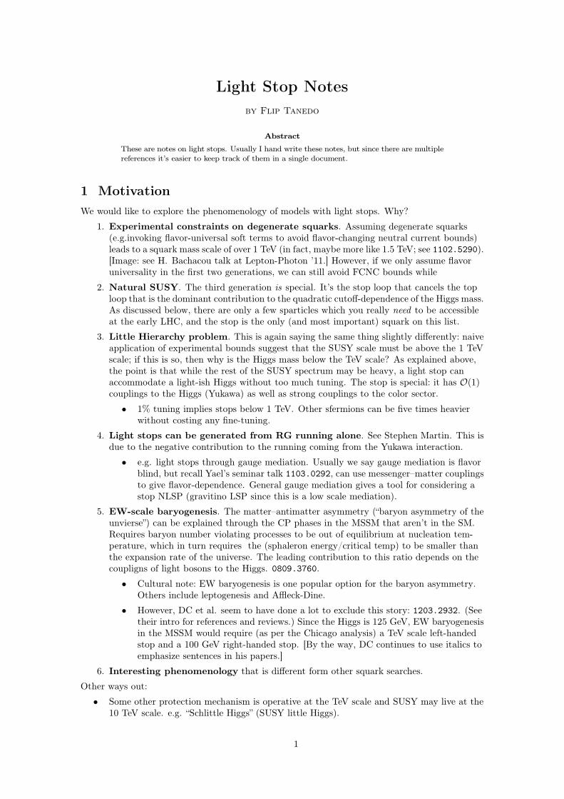
4.5.3 Kinematic distributions

As before, the main background comes from ditop. Katz and Shih give kinematic distributionsfor sample stop masses (from 120 to 200 GeV) relative to the ditop background for:

• Lepton pT

• b-jet pT : stops lighter than the top give softer b-jets.

• MET (all hadronic, lepton+jets, dilepton)

• mT : stops have a high mT tail in the leptons+jets channel.

• HT (scalar sum of jet pT ): somewhat lower values for HT for stops in leptonic channels

• mℓb (invariant mass of lepton and b-quark at parton level) for different lepton pairings. Notethat this is not currently used in any exisiting analyses (as of the writing of that paper) andcan be a useful distinguishing variable.

I really can’t tell by eye if these distributions are discriminating... doesn’t look like it, and anywayit’s clear that there are limits where the stop looks very much like a top.

For stops lighter than the top, the b-jets are much softer due to kinematics. This is due to aJacobian peak in pbT in the top frame when there is an on-shell top. On the other hand, for the3-body decay (from the 4-point interaction), the distribution is different.

4.5.4 Comments from Peskin and Chou (’99)

Here’s a plot from Peskin and Chou hep-ph/9909536 with the distribution of mℓb. Plotted are astop with mass 130 GeV (dotted) and 170 GeV (dashed) for a scenario where the lightest charginois light (m2∼ 200 GeV) and wino-like. The solid line is the meb spectrum for a top quark. Thedistribution has good discriminating power against tops.

Unfortunately, the other scenarios that they present (Higgsino like lightest chargino, mixedlightest chargino, heavy lightest chargino) do not give as much separation between the distribu-tions.

Another handle they present is the longitudinal W polarization. Top decays tend to be highlylongitdinally polarized. In the SM,

r=Γ(W0)

Γ(Wall)=

1

1+ 2mW2 /mt

2 ≈ 0.71.

In the light stop scenario, this ratio is a function of the chargino mixing matrices. The point,however, is that one can variations between r= 0.4 and 0.9.

Phenomenology: searches for stops 9

4.5.5 Searching for stop NLSP, part I: Ditop analyses

The first class of searches are those where the stop events are hidden in the ditop data. The hopeis that we would just have to see a deviation from what we expect. In the next sub-sub-section wediscuss explicit stop searches. The hidden-in-the-top-data searches can be categorized based onthe W decays:

• Dileptonic (5%): 2 leptons, 2 jets, MET. Cleanest, S/B∼2. However, very small branchingratio so that the statistical uncertainty is roughtly of the same size as the systematic.

• Lepton + jets (35%): Larger branching ratio, but large W+jets background—require b-tag to beat this down.

• Jets + MET (10%): zero lepton events where at least oneW decays to τν with τ→hadrons.QCD background is hard. Most stops fall in this category due to gravitino. Cut and countis no good against the QCD background, but more sophisticated neural network techniquesmay be helpful. The CMS group is working on something along these lines with a giantmaximum likelihood calculator.

• Fully hadronic (50%): QCD background is hard.

A typical set of requirements (lepton, 4+ jets, MET) lead to S/B∼4 with systematic uncertainty2× statistical. Katz and Shih explain that many additioanl top quark properties are not as usefulas one would hope since they use matrix elements or neural networks to kill background andare thus likely to discriminate against stop events as well. Other properties require an accuratereconstruction of the ditop event so that the stop events (with missing momentum due to thegravitino) tend to be rejected as background. More practically, since the experimentalists’ codesare proprietary, it is inaccessible to phenomenologists.

4.5.6 Searching for stop NLSP, part II: explicit stop searches

The GMSB-inspired stop NLSP scenario presents some opportunities for novel experimentalsearches. Some of these searches can be reinterpreted from existing ditop-like signatures.

• Stop decay via virtual chargino, t→ bℓ+ν . 1009.0266, 0811.0459, D0 Note 5937-CONF,

1009.5950. The neutrino can either be the LSP or can decay invisibly the a neutrino and

a neutralino/gravitino. Signatures are similar to the t→W+b G decay dilepton channel.

• Another ditop-like signature is t→ b(

χ1+→W (∗)νχ1

0)

.

• A similar signature is t→ b(χ1+→ℓνχ1

0). 0912.1308, CDF Note 9439, FERMILAB-THESIS-

2010-16. CDF has an algorithm to reconstruct the stop mass which helps discriminateagainst top events. However, there are four invisible particles and two particles (charginoand neutralino) with unknown mass, the reconstruction is imperfect. With an assumptionfor the chargino mass, there is a stop-mass-like quantity that they can construct which hasa distribution which is peaked roughly at the stop mass.

• Other searches: b-jets + MET 1103.4344, search for heavy top partner ATLAS-CONF-2011-036.

4.5.7 Searching for stop NLSP, part III: other searches

We now consider some additional regions of stop NLSP parameter space.

• Displaced decays. The stop can be naturally long lived. For decays between 100 µm and0.5 m from the interaction point, a displaced vertex can be tagged. One can avoid heavyflavor displaced vertices (background) by looking at distances above 1 cm, for which thismay be uased as a discriminator against the Standard Model. Stops hadronize, possibly intocharged particles which leave tracks with large amounts of energy lost through ionization.

• Stoponium. One can form a near-threshold stop bound state. The annihilation rate intogg can be of order Γ−1∼ 10−13 m, for nearly degenerate top and stop. Stopnoium wouldgive a diphoton resonance that could allow a precise stop mass measurement in a few yearsat the LHC.

10 Section 4

• Flavor violation, SS2L. Stop to charm and neutralino/Gravitino may become a dominantdecay if there are new sources of flavor violation. In this case, the Tevatron could excludestops up to 180 GeV if mt −mχ

0 & 50 GeV. With even small flavor violation, mesinooscillations hep-ph/9909349 can convert stops into antistops and lead to same-sign dileptonevents with jets and MET. See also 1207.6794 for t→ ch, which may be relevant.

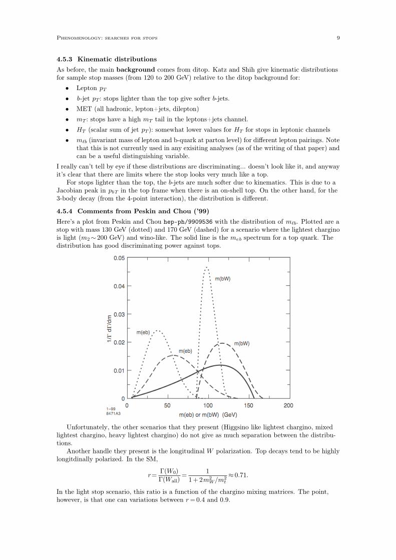
4.6 Bump hunting

Brust, Katz, and Sundrum presented a bump search for RPV models 1206.2353. In these models,the stop is indeed the LSP, but this decays into two jets via the RPV coupling ∆W ⊃ tRdRdR.(These RPV couplings individually have to be so small to avoid proton decay and flavor boundsthat it’s sufficient just to turn on one coupling at a time.) This means that you can get signatureswhich are devoid of MET and leptons. Existing cut and count searches aren’t optimized for thissort of signal since they miss out on the dijet decay.

The BKS paper presented an alternate search based on reconstructing the resonances of thedijet decay of the stops. They consider cascade decays of heavier squarks into the light stops. Theyfocus on sbottom decays rather than heavy stop decays since the latter decays are more model-dependent: the heavy stop to light stop-Z and light stop-h decays depend on the left-right stop

mixing. Meanwhile, they focus on: b→W (∗)t . The strategy is:

1. Tag events with two isolated leptons and “moderate” MET (to kill the Drell-Yan dileponcontribution)

2. Cluster the jets with a large radius. If you miss jet components then you can’t reconstructthe resonance.

3. If the event contains 4+ jets, then we have to play combinatoric games. Since we assume thatthese jets come from the light stops, we can bias our combinatoric searches by minimizingthe difference between reconstructed invariant masses.

Background: top pair production with dileptonic decays (100× signal), but one can cut awaymost of the other backgrounds. So one has to use an additional discriminator: the hardness of theevent. In ditop events, the hardness of the event correlates with the hardness of the leptons andMET. In the signal, however, there may only be a mild splitting between the stop and sbottom(by assumption in the model) so that typically one cannot emit an on shell W . This means there’srelatively low lepton pT and MET even if the overall event is hard. So the simplest thing to do is tocut the high MET and high lepton pT tail. One can do better, however, by defining dimensionlessvariables in where these quantities are scaled by the total event hardness.

4.7 Light [Stealth] Stop Signs 1205.5808

Harvard group. Focuses on the stealth stop window, mt.mt . 250 GeV, look for new handles onthis difficult region. The difficulty, recall, comes mainly from the fact that these stops decay intostops and a relatively soft neutralino/gravitino so that these effectively look like top decays.

Note that at 7 TeV, the stop cross section is only a sixth of the top cross section for degeneratestop/top. This drops rapidly for larger masses. Thus we need as many handles as we can get sincesimply measuring the total rate for events passing top selection is not enough.

4.7.1 Spin semi-correlation

The most important fact of the stealthy regime is that stops are spin zero and are produced withoutspin correlations. Thus the stop and antistop decays are completely uncorrelated. What does thisbuy us?

Suppose we have a sample of ‘top’ events which include stealthy stops. The real top decays arespin correlated, while the stops slightly wash out this correlation. Melnikov and Schulze 1103.2122showed that these correlations are stable with respect to NLO corrections, which is a uniqueproperty for our handles of stealth stops.

They focused on looking at, for example, the distribution of ∆φ(ℓ+, ℓ−). I’ll not go into thisfurther since spin correlation techniques are a whole separate bag of worms. See the paper for adiscussion and references.

Phenomenology: searches for stops 11

4.7.2 Stop versus top production

The stop production rate is suppressed relative to the top production near threshold. There aretwo reasons for this.

1. gg→tt has t- and u-channel singularities which are regulated by mt. On the other hand,di-stop production does not have such a singularity. This is because the only diagram whichlooks like it could give such a singularity. This can lead to the use of a rapidity gap as adiscriminator. This explains why the gg production channel for tops and stops are different(68 pb vs 11 pb).

2. Stop production is p-wave in the s-channel (that’s a confusing way of saying it) productionfrom the qq initial state. This is because the stop final states must carry angular momentum;the production goes through an s-channel gluon which is spin-1. This means the productionrate goes like β3 (where β is the velocity) near threshold. This suggests looking at higherpT where stop production might be enhanced. This, however, is less interesting at the LHCdue to the parton PDFs. This explains why the q q production channel for tops and stopsare different. (23 pb vs 1.6 pb.)

Indeed, the stop production cross section from gluinos is given to leading order by:

σ(

gg→t t∗)

=αs

2π

s

[

β

(

5

48+

31m2

24s

)

+

(

2m2

3s+m4

6s2

)

log1− β

1 + β

]

where β2 =1− 4m2/s is the subprocess velocity.

4.7.3 Rapidity Gaps

The gluon to (s)top production cross sections are, in the massless limit:

σ(stop) =5αS

2π

48s

σ(top) =αS

2

24s(t2 + u2)

(

1

tu− 9

4s2

)

.

The top singularities are regulated by the top mass so that it ends up being log s/mt2 enhanced.

You can also see this using MHV amplitudes,

M(1+, 2−, 3ϕ, 4ϕ) = ie2[13]〈23〉〈13〉[23]

= e2× phase

M(1+, 2−, 3−, 4+) = ie2[14]〈23〉〈13〉[23]

= e2u

t

√

× phase.

They note that the top production case corresponds to the “familiar splitting function amelioratingthe ple in a t-channel diagram to the squareroof of a pole in the amplitude.” The two results arerelated by a SUSY Ward identity.

They then look at the effect of this on the rapidity distribution ∆y between the top and anti-top.They noted that the effect of the shape can be mimicked by increasing the renormalization scale.

4.8 Kinematic variables with endpoints for background

“Stop the top background,” Bai, Cheng, Callicchio, and Gu. 1203.4813.

4.9 Tagging boosted tops from stop decay

• 1205.5816: Stolarski, Kaplan, and Rehermann.

12 Section 4

• 1205.2696: Plehn, Spannowski, Takeuchi.

4.10 MET and MT shapes

1205.5805. Alves, Buckley, Fox, Lykken, Yu (Tien-Tien).

5 Review of Work: UV theories

Common theme: the third generation is special through compositeness. Otherwise you have tofigure out a way to explain flavor structure; compositeness does this ‘automatically’ e.g. througha small splitting in anomalous dimensions at the high scale.

5.1 Supersymmetric warped extra dimension

Uses XD localization and ‘emergent’ (See below) or ‘partial’ supersymmetry hep-ph/0302001.

• General problem: gauginos are external to the strong dynamics (compare to McSSM) andneed to be both light and have supersymmetric couplings to avoid dangerous quadraticdivergences in the Higgs mass. However, the gauginos are part of the elementary sector(which feels SUSY breaking strongly) and neither assumption holds automatically, requiringsome model building.

• Automaticatically inherits nice features of RS: e.g. hierarchical Yukawas

•

5.1.1 Emergent SUSY 0909.5430

Stringily-motivated; suppose SUSY is high scale but “vestiges” of supersymmetry are ’accidentally’redshifted down to the TeV scale. In the dual sense, this is emergent/accidental supersymmetryin the strong sector. SUSY no longer solves the big Hierarchy problem (which is now solved bywarping), but it does address the Little Hierarchy problem.

• Goes on to extend this idea: replace non-SUSY weakly coupled sector with the weakly-cou-pled sector of split supersymmetry: light gauginos. Suppresses dominant Higgs radiativecorrections in the little Hierarchy.

• Higgs is a composite state whose mass happens to be light compared to the dynamical scale.(The usual problem in composite models.) Introduces a ‘little’ µ-problem, despite beingtechnically natural.

• Also became a prototype for his effective SUSY work with Katz et al.

5.1.2 Partially supersymmetric, pseudo-Goldstone Higgs 1004.5114

By Redi and Gripaios. Supersymmetric Randall-Sundrum. Understood to be SO(5)/SO(4) pseudo-Goldstone Higgs. Maps onto the ‘More Minimal SUSY’ic SM.’ Different from Raman’s model inthat it’s really supersymmetrizing the minimcal composite Higgs model. Thie Higgs only couplesderivatively to the strong sector, Yukawas obtained through mixing with elementary sector.

• Regarding gaugino problem: assume SUSY breaking in elementary sector is large com-pared to the compositeness scale but soft, so couplings are approximately supersymmetric.Gaugino masses then require an approximate R-symmetry that is respected by SUSYbreaking.

• Generation of Higgs potential is different from non-supersymmetric case. In minimal com-posite Higgs, required Higgs potential to come from loop-level couplings to fermions (e.g.top). However, for the SUSY MCH, a quartic of the correct order of magnitude is auto-matically generated and mass terms are only generated at loop level when SUSY is broken.This avoids problems composite Higgs models that have a high compositeness scale.

Review of Work: UV theories 13

5.2 Deconstructed third generation 1103.3708

See Jack’s talk last year. The quiver diagram can be understood as a deconstruction of the generalframework above.

5.3 Composite MSSM 1201.1293

Another handle on strong coupling is Seiberg duality. This is again a variation of the same themeabove.

See my separate notes on McSUSY. For references see arXiv:1106.3074 (Csaki, Shirman,Terning, “A Seiberg Dual for the MSSM”) and arXiv:1201.1293 (Csaki, Randall, Terning, “LightStops from Seiberg Duality”). For background, see my Seibergology notes.

5.4 Flavor mediation 1203.1622

Explicit flavor structure introduced in messengers. For related ideas, see Yael’s seminar talk lastweek.

6 Experimental bounds

6.1 General squarks

Searches for first and second generation squarks have been very restrictive. However, as weexplained above, these bounds have essentially no impact on fine-tuning in the MSSM.

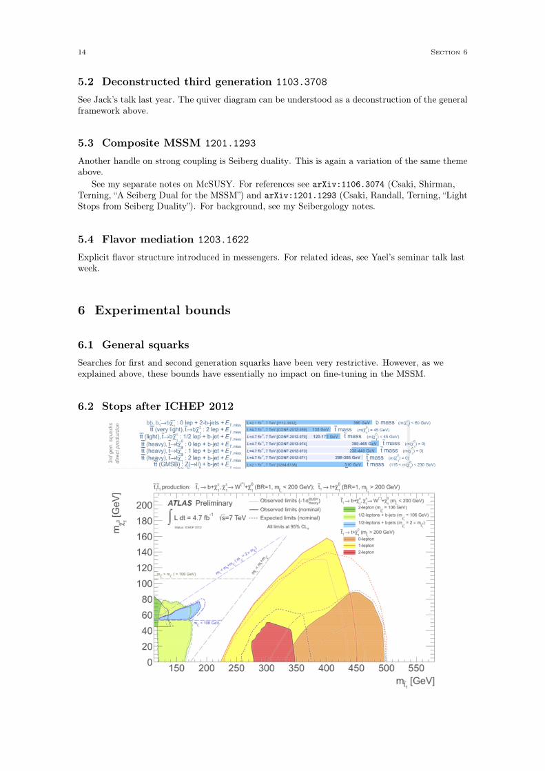
6.2 Stops after ICHEP 2012

14 Section 6

6.2.1 ATLAS-CONF-2012-059: 7 TeV 4.7/fb

Search for light stops.

Signal: 2 leptons + jets + MET

Bounds: assuming t→ bχ+ with mχ+ = 106GeV, fixes mt > 130GeV for mχ0< 65GeV.

6.2.2 ATLAS-CONF-2012-070: 7 TeV 4.7/fb

Search for light stops with mass around (or lighter) than the top mass. Look for one or two leptons,large MET, light flavor jets, and b-jets.

Signal: 1 or 2 leptons + 1 or 2 b-jets + jets + MET

Bounds: Assuming t→ bχ+. Excludes 120GeV<mt <mt for mχ0∼ 55GeV.

6.2.3 ATLAS-CONF-2012-071: 7 TeV 4.7/fb

Search for medium-mass stop partners decaying to t and neutral non-interacting particle. Sensitiveup to stop masses up to 200 GeV. Direct pair production of top partners (stop or spin-1/2 partner)

with t→ tχ0. Look for two leptons in final state.

Signal: 2 leptons + jets + MET.

Bounds: Rules out a mt ≈ 300GeV decaying to a massless neutralino, assuming a signal thatis 1σ below the central value.

6.2.4 ATLAS-CONF-2012-073: 7 TeV 4.7/fb

Search for direct heavy stop production; events with an isolated lepton, jets, and MET, witht→ tLSP.

Signal: 1 lepton + jets + MET

Bounds: Rules out 230GeV<mt < 440GeV for massless LSP.

6.2.5 ATLAS-CONF-2012-074:

Heavy stop assuming t→ tLSP with both quarks decaying hadronically.

Signal: 0 lepton + jets + MET

Bound: excludes 370GeV<mt < 465GeV for massless LSP.

6.3 Stop NLSP

See the Stop NLSP section above for the Katz and Shih analysis of past Tevatron and LHC bounds.Here we review their section 4, which describes some of the current (at the time) bounds on thestop NLSP scenario.

The searches which are most sensitive are those which:

• are more accepting of soft jets, or

• use more discriminating variables such as mT or some kind of reconstructed stop mass.

6.3.1 Cut and count

The expected number of stop events is

Nt t∗ =

(

εt t∗

εtt

)

×(

σt t∗

σtt

)

×Nt t.

The first factor is the relative acceptance for stop pair production. The second factor is the relativeproduction cross section. Armed with this information, one can calculate exclusion confidencelevels. Here are the results:

Experimental bounds 15

Remarks on the self-consistency of their simulations:

• The use of these ratios and Ntt cause many systematic errors in the simulations to cancel.(This is a sanity check for the results.)

• Raw number Ntt agrees with experimental references at 30%.

• The stop cross section has a power law dependence on the stop mass, but the stop limitsare not appreciably changed by 10% changes in the acceptance in either direciton.

Results, very light stops ∼120 GeV

• Acceptance is affected significantly by the requirements on number and ET of jets. Lightstops tend to decay into soft b-jets.

16 Section 6

• The acceptance is close to 1 only for the D0 stop search since it does not impose a require-ment on the number of jets. This gives it the best cut-and-count exclusion for a 120 GeVstop.

• The b-tagged sample in the CDF search is relatively high, while other analyses have stricterjet ET requirements leading to lower acceptences.

Results, ∼150 GeV intermediate mass stops

• b-jets are harder and are more efficient in passing selections, but reduced cross sectionsweaken the limits.

• ATLAS top partner search for leptons + jets has high acceptance because it cuts on mT >

120 GeV, which elminates the top backgroun.

• O(100)/pb data should be able to reach 95% CL exclusion for stops up to 180 GeV, butbeyond this one is limited by systematic errors.

6.3.2 Stop mass reconstruction

Based on 0912.1308, CDF Note 9439, FERMILAB-THESIS-2010-16, which uses a dilepton stopmass reconstruction algorithm at CDF. The algorithm assumes a stop decay t→ bχ+→ ℓνbχ0,but turns out to work also for the stop NLSP scenario by giving a much sharper mass distributioncompared to the top that is centered at a different value. It seems like Katz and Shih mapped onstop NLSP parameter points to similar gravity mediated parameter points so that they could usethe CDF analysis.

The result of this analysis gives a stop NLSP exclusion for mt <150GeV. This is the best limitin their paper. “This illustrates the power of using more discriminating variables in searching fornew physics in the ditop sample.” Future directions include using the D0 stop search (which theycould not reinterpret because it would require access to their data).

6.3.3 Other types of measurements

• Invariant mass of the lepton-b system. (See hep-ph/9909536) Can reduce ditop background.Ambiguities in pairing lepton and b-jet, but even incorrect pairing contributes in a similarway to the differences between distributions. This distrubtion has not been published (asof the Katz-Shih paper) since the 700/pb data from the Tevatron.

• b-jet pT distribution. Is there a way to use the softness of b-jets from stop decay to separatethe ditop background? Limiting factors: pT > 12GeV for proper reconstruction of b-jet pTand efficiency decreases with pT .

• Displaced decays. No dedicated searches as of the time of the Katz/Shih paper, thoughyou can find some ideas from searches for hidden valley scenarios. Current ATLAS and CMSstudies for charged stop-hadrons are not constraining due to the requirements of each search.

6.4 The gluino

Current bounds (from Han, Katz, Krohn, Reece) push the gluino above ∼900 GeV.

• ATLAS-CONF-2012-004: two same-sign leptons, jets and missing transverse momentum

• 1205.3933: CMS, same-sign dileptons and b-tagged jets

• CMS-PAS-SUS-11-027: single lepton and jets using templates

• ATLAS-CONF-12-037: large jet multiplicities and missing transverse momentum

6.5 Flavor/Naturalness bounds on stop mixing

6.5.1 1206.5303: IAS Higgs couplings from natural SUSY

Defines ratio of Higgs couplings to SM values:

ri=ghii

ghiiSM.

Experimental bounds 17

Writing Xt=At− µ/tan β, we have rG= rtrGt with

rGt − 1≈ 1

4

(

mt2

mt12 +

mt2

mt22 − mt

2Xt2

mt12 m

t122

)

+ (D− term contribution)

This can give a substantial effect for reasonably light (≈250GeV) stops: rG=1.24. This would givea 53% increase in gluon fusion Higgs production. A large stop mixing, however, could reduce thiseffect. This is limited by naturalness: a large Xt contributes to the weak scale tuning directly andthrough the requirement of larger diagonal soft masses.

Stronger constraints for stop mixing come from B→Xsγ, which only allows new physics tocontribute at about 30% of the loop-suppressed SM contribution. To avoid large tree-level SUSYcontributions, it is typical to assume parameters in which such contributions cancel and measurethe fine tuning. The result of the IAS group analysis is that to avoid cancellations to a level in onepart per ten, we must have Atµ tan β/m t2< few.

6.6 Fits to Higgs decay channels

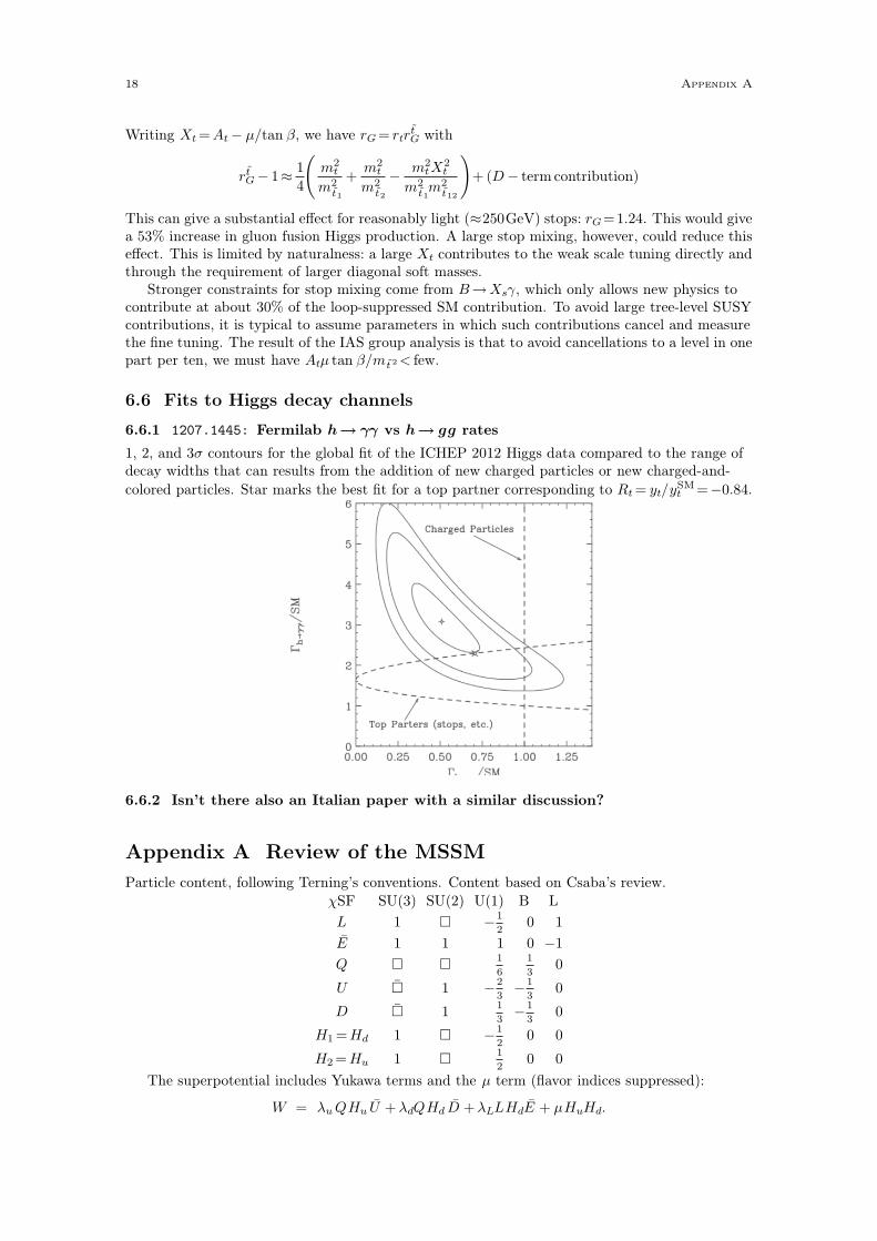
6.6.1 1207.1445: Fermilab h→ γγ vs h→ gg rates

1, 2, and 3σ contours for the global fit of the ICHEP 2012 Higgs data compared to the range ofdecay widths that can results from the addition of new charged particles or new charged-and-

colored particles. Star marks the best fit for a top partner corresponding to Rt= yt/ytSM=−0.84.

6.6.2 Isn’t there also an Italian paper with a similar discussion?

Appendix A Review of the MSSM

Particle content, following Terning’s conventions. Content based on Csaba’s review.

χSF SU(3) SU(2) U(1) B L

L 1 � −1

20 1

E 1 1 1 0 −1

Q � �1

6

1

30

U � 1 −2

3−1

30

D � 11

3−1

30

H1 =Hd 1 � −1

20 0

H2 =Hu 1 �1

20 0

The superpotential includes Yukawa terms and the µ term (flavor indices suppressed):

W = λuQHu U +λdQHd D +λLLHdE + µHuHd.

18 Appendix A

On top of this, the following terms are B or L violating and are removed by R-parity which isdefined in terms of B, L, and the spin S by R=(−)3B+L+2S,

WR =α1QL D +α2LL E +α3LHU +α4 DDU .

Appendix B MSSM Higgs scalar potential

One of the most important parts of the MSSM is the scalar potential for the Higgs and theconstraints from the requirement of electroweak symmetry breaking. See hep-ph/9606414 fordetails.

B.1 Supersymmetric contribution

Recall that the general form of the scalar potential for a renormalizable supersymmetric theory is

V (φ)=Wi∗W i+

1

2

∑

a

ga2(φ∗T aφ)2,

where the first term is the F -term contribution and the second is the D-term contribution. Fromthe superpotential we can see that only the µ-term contributes to to F -term potential since thesfermions don’t get vevs:

∆VF(Hu, Hd)= |µ|2|Hu|2 + |µ|2|Hd|2.The D-term potential is simpilified using σijσkl= 2δilδjk− δijδkl,

∆VF(Hu, Hd) =1

2g2(

Hu∗σ

2Hu

)

2+

1

2g ′2|Hu|4 +(u→ d)

=1

2g2(2|Hu

+|2|Hu0|2− |Hu

0|2|Hu+|2) +

1

2g ′2(|Hu

0|2 + |Hu+|2)+ (u→ d,+→−)

=1

8(g2 + g ′2)(|Hu

0|2 + |Hu+|2− |Hd

0|2− |Hd−|2)2 +

1

2g2|Hu

+Hd0∗+Hu

0Hd−∗|2.

B.2 Mass matrix in SUSY limit

Now let us write out the mass matrix for a complex scalar field φ in the basis Φ=(φ, φ∗)T so thatthe mass matrix M2 appears as

1

2Φ∗M2Φ. Sub/superscripts i, j , k refer to derivatives with respect

to φ or φ∗ respectively, while subscripts a refer to the gauge group.

(M2)ij =

W ikWkj+1

2DaiDaj+

1

2(Da) j

iDa W ikjWk+1

2DaiDa

j

W kWikj+1

2DaiDaj W jkWki+

1

2Dai Daj+

1

2(Da) j

iDa

B.3 SUSY breaking contributions

We now include soft SUSY breaking terms. These come in the form of holomorphic masses (Bterms) and soft masses. (There are no holomorphic trilinear A terms by gauge invariance.)

∆Vsoft(Hu, Hd) = mHu

2 (|Hu0|2 + |Hu

+|2)+mHd

2 (|Hd0|2 + |Hd

−|2)−Bµ(Hu ·Hd)

= mHu

2 (|Hu0|2 + |Hu

+|2)+mHd

2 (|Hd0|2 + |Hd

−|2)−Bµ(Hu+Hd

−−Hu0Hd

0 + h.c.)

where we’ve written the B term with a factor of µ pulled out as a choice of convention. Note thatit is also standard to write b=Bµ (e.g. Stephen Martin’s review).

B.4 Total Higgs scalar potential

As written in Martin’s review (eq. 8.1.1 in version 6):

V = (|µ|2 +mHu

2 )(|Hu0|2 + |Hu

+|2) + (|µ|2 +mHd

2 )(|Hd0|2 + |Hd

−|2)+[b(Hu

+Hd−−Hu

0Hd0)+ h.c]

1

8(g2 + g ′2)(|Hu

0|2 + |Hu+|2− |Hd

0|2− |Hd−|2)2 +

1

2g2|Hu

+Hd0∗+Hu

0Hd−∗|2

MSSM Higgs scalar potential 19

B.5 Electroweak symmetry breaking

[I’ve been sloppy with the sign of b, sorry.] Note that the supersymmetric potential isleads to a positive definite mass matrix whose vev is 〈Hu〉= 〈Hd〉=0. Note, further, that we need

〈Hu+〉= 〈Hd

−〉= 0; in the followingwewriteH for H0 for simplicity. In order to break electroweaksymmetry, we need the soft SUSY breaking terms. Introducing some notation, the form of ourpotential is:

V = mH1

2 |Hd|2 +mH2

2 |Hu|2−m122 (HuHd+ h.c.) + (D terms).

One may worry about the negative contribution coming from the m122 piece. The quartic contri-

bution from the D term (given above) vanishes in the direction |Hu|= |Hd| (they are “D-flat”), sothis is a legitimate concern. In order for the potential to be bounded from below in this direction,we thus require

mH1

2 +mH2

2 > 2|m122 |.

mH1

2 = |µ|2 +mHd

2

mH2

2 = |µ|2 +mHu

2

m122 = b=Bµ

Observe that b=Bµ alsways favors electroweak symmetry breaking. The D term contributionsare given above. Requiring that we get a negative squared mass near Hu=Hd= 0 for one linearcombination gives (by taking the determinant of the mass matrix)

b2>mH1

2 mH2

2 .

You might worry that this is only sufficient and not necessary since one might have the mass matrixhaving two negative eigenvalues. However, the previous conditionmH1

2 +mH2

2 >2|m122 | enforces that

the trace of the mass matrix is positive. Thus EWSB requires that the mass matrix has exactlyone negative eigenvalue. (Thanks to the Sparticle book for spelling this out.)

We thus have the bounds:

1. 2b<mHu

2 +mHd

2 + 2|µ|2

2. b2> (|µ|2 +mHd

2 )(|µ|2 +mHu

2 ).

These relate supersymmetric in the superpotential to soft breaking terms, parameters which a

priori are expected to be unrelated. Note that there is no solution for mHu

2 =mHd

2 , if one expectsthese two to be equal at a high scale, then electroweak symmetry is unbroken at tree-level.

Comments on RG: One can consider the RG running of these parameters from the high scaledown to the weak scale. A reasonable assumption is to only include the top Yukawa coupling and

the gauge interactions. The relevant expressions are the β-functions for mH2

2 , mt2, and mQ3

2 . These

are functions of the gaugino masses, the gauge couplings, the top Yukawa, and the top A-term.The main story is this: (see hep-ph/9606414): Loops involving the top Yukawa coupling want tomake the up-type Higgs mass negative, this is indeed what we want for EWSB.

Let us assume that the neutral component of the Higgs doublets obtain vevs vu and vd. As

usual, we define v2 = vu2 + vd

2 =2mZ2 /(g2 + g ′2)= (174GeV)2 and tan β= vu/vd. These vevs can be

chosen to be real and positive. Using these relations we can write ∂V /∂Hu,d0 = 0:

∂V

∂Hu0

= 2mH2

2 vu− 2bvd+1

2(g2 + g ′2)(vu

2 − vd2)vu

= 2vu

(

|µ|2 +mHu

2 −b cotβ+mZ

2v2(vu2 − vd

2)

)

= 2vu

(

|µ|2 +mHu

2 −b cotβ − mZ

2cos 2β

)

.

Similarly for ∂V /∂Hd0, with a minus sign on the final term. We end up with the conditions:

mHu

2 + |µ|2− b cot β− mZ

2cos 2b = 0

mHd

2 + |µ|2− b tan β+mZ

2cos 2b = 0.

20 Appendix B

It is common to rearrange these into constraints on the parameters:

|µ|2 =mHd

2 −mHu

2 tan2β

tan2β − 1− 1

2mZ

2

b =(mHu

2 +mHd

2 +2|µ|2)sin 2β

2|µ| .

MSSM Higgs scalar potential 21