i

Limitations of the Ground

Reaction Curve Concept for

Shallow Tunnels Under

Anisotropic In-situ Stress

Conditions

Diego Lope Álvarez

Master of Science Thesis in

Soil and Rock Mechanics

Stockholm, Sweden, 2012

Limitations of the Ground Reaction

Curve Concept for Shallow Tunnels

Under Anisotropic In-situ Stress

Conditions

Diego Lope Álvarez

Master of Science Thesis 12/07

Division of Soil and Rock Mechanics

Department of Civil and Architectural Engineering

Stockholm, Sweden, 2012

Source of the cover picture: Skanska Sverige A.B.

i

ACKNOWLEDGEMENTS

This master level degree project was carried out from January 2012 to June 2012 at the

Department of Civil and Architectural Engineering in the Royal Institute of Technology – KTH

(Stockholm, Sweden).

First of all, I would like to express my gratefulness to my supervisor Dr Fredrik Johansson, for

his invaluable advices, patience and encouragement throughout this work.

Special thanks are also acknowledged to Diego Mas Ivars, who initiated the project and

provided me invaluable advices not only for this work, but for my future career. Throughout

the numerical implementation of the model, Abel Sanchez Juncal has helped out with valuable

information and knowledge about UDEC. I would also like to thank them for introducing me in

the amazing field of rock mechanics.

Thanks also to Itasca Consultants, for allowing me to do this work sitting at its office in

Stockholm and using its software UDEC 5.0, I felt as one more of the members of such amazing

team.

I would like to express my gratitude to my mother (Gracias, mamá!), to my sister, and to also

my friends in Spain, because I am totally sure that they have missed me these months.

Last but not least, I would like to thank the friends that I have met during this year, especially

Norrtälje’s ones, because they have become my “new family” during the last 10 months in

Sweden.

Diego Lope Álvarez

Stockholm, June 2012

ii

ABSTRACT

The deep mining industry and civil engineering need to perform rock stability analyses during

excavation projects. These analyses are closely related with displacements in tunnel contours.

The ground reaction curve is a powerful tool to characterize these displacements that is widely

used in the New Austrian Tunneling Method. However, the analytical solutions that exist are

only applicable under isotropic stress conditions for deep tunnels.

This study aims to investigate when it is possible using the analytical methods to determine

the ground reaction curves with enough accuracy in the case of shallow tunnels under

anisotropic in-situ stress conditions.

The method begins with a literature study. After that, with the help of a 2D model, a

comparison between the analytical and the numerical solutions for ground reaction curves at

different depths and at different initial in-situ stress ratios was carried out.

The results show that both crown and floor displacements deviate more from the analytical

solution than the wall displacement. The crown and floor can even move upwards under high

initial in-situ stress ratios for shallow tunnels. Because of that, the analytical solution of the

ground reaction curve at shallow depths under anisotropic stress conditions should not be

used.

In the case of isotropic stress field conditions for the analysis in this study, the results given by

the analytical solution agree with the numerical ones at depths higher than 14 times the radius

of the tunnel. On the other hand, the difference between numerical and analytical solutions

becomes higher while increasing the initial in-situ stress ratio, even for very deep tunnels.

Furthermore, an empirical equation to obtain the displacements of the ground surface, tunnel

wall and tunnel crown has been obtained after a multiple linear regression analysis.

Keywords: Ground reaction curve, shallow tunnels, isotropic stress conditions, anisotropic

stress conditions, analytical solution.

iii

SUMMARY

Difficulties in determining in-situ stresses in the firsts tens of meters below ground surface

together with the fact that available analytical solutions are not applicable for shallow tunnels

under anisotropic conditions has motivated this study. The problem was also given additional

interest in connection to the increasing number of shallow tunnels under construction in the

area of Stockholm.

Because of that, the aim of this master thesis is to investigate the shortcomings of the ground

reaction curve for tunnels at shallow depths and high initial in-situ stress ratios. In order to

investigate that, a 2D distinct element analysis was carried out by UDEC 5.0. In this analysis, a

tunnel placed at four different depths and with several different initial stress ratios was firstly

analyzed. Thereafter, the ground reaction curves were plotted and analyzed in detail. The

investigation also concerns the possibility of determine empirical equations to estimate the

final displacements of the tunnel contour and ground surface for those conditions.

This thesis shows that the problem of obtaining ground reaction curves in shallow tunnels is

complex. In the case of isotropic stress field conditions, the results given by the analytical

solution agree with the numerical ones at depths higher than 14 times the radius of the tunnel.

On the other hand, the difference between numerical and analytical solutions becomes higher

while increasing the initial in-situ stress ratio, even for very deep tunnels. The conclusion of

this is that the analytical solution should not be used neither for anisotropic in-situ stress fields

nor shallow tunnels.

One of the main findings was that the depth of the tunnel does not influence as much as the

initial in-situ stress ratio does. Another finding is that the crown and floor displacement

deviate more from the analytical solution than the wall displacement. Both crown and floor

can even move upwards under high in-situ stress ratios acting. As expected, the excavation-

induced decline to the in-situ stresses at an approximate distance of three tunnel diameters,

even for cases with high initial in-situ stress ratios.

Finally, the study suggests that the displacements in the tunnel wall, tunnel crown and ground

surface under anisotropic conditions can be roughly estimated with a proposed equation, but

further research is necessary in order to estimate displacements more accurately.

iv

SYMBOLS AND NOTATIONS

Commonly used symbols and notations are presented below

Roman letters

area [m2]

cohesion [Pa]

Young’s modulus of elasticity [Pa]

Young’s modulus of the earth crust [Pa]

yield criterion

shear modulus [Pa]

acceleration of gravity [ms-2]

stiffness matrix

hardening modulus

initial stress ratio

initial pressure [Pa]

pressure at point i [Pa]

plastic potential

radius [m]

displacement [m]

displacement of the tunnel wall [m]

depth [m]

Greek letters

unit weight [Nm-3]

strain

hardening parameter

plastic multiplier or UDEC displacement/analytical displacement

Poisson’s ratio

density [kgm-3]

major principal stress [Pa]

minor principal stress [Pa]

uniaxial compressive strength [Pa]

horizontal stress [Pa]

tensile strength [Pa]

vertical stress [Pa]

normal effective stress [Pa]

shear stress [Pa]

dilation angle [ ]

friction angle [ ]

v

CONTENTS

ACKNOWLEDGEMENTS .........................................................................................................i

ABSTRACT ........................................................................................................................... ii

SUMMARY ......................................................................................................................... iii

SYMBOLS AND NOTATIONS ................................................................................................. iv

1. INTRODUCTION ............................................................................................................... 1

1.1 Background.............................................................................................................................. 1

1.2 Aim .......................................................................................................................................... 1

1.3 Disposition ............................................................................................................................... 2

1.4 Limitations ............................................................................................................................... 2

2. LITERATURE STUDY .......................................................................................................... 3

2.1 Introduction............................................................................................................................. 3

2.2 Fundamental principles of in-situ stresses .............................................................................. 3

2.3 Rock mass material models ..................................................................................................... 5

2.3.1 Introduction.................................................................................................................. 5

2.3.2 Material behavior models ............................................................................................ 6

2.3.3 Mohr-Coulomb failure criterion ................................................................................... 7

2.3.4 Modeling a continuum material ................................................................................... 7

2.3.5 Failure modes in tunnels ............................................................................................ 10

2.4 Shallow tunnels vs. deep tunnels .................................................................................. 12

2.5 Calculation methods ............................................................................................................. 13

2.5.1 Introduction................................................................................................................ 13

2.5.2 Analytical method: Convergence confinement method ............................................ 13

2.5.3 Ground reaction curve as part of CCM ....................................................................... 14

2.5.4 Numerical methods .................................................................................................... 17

2.6 Practical applications of the approach .................................................................................. 18

2.5.1 Limitations .................................................................................................................. 18

2.5.2 Tunnel with non-circular section and anisotropic stress field ................................... 18

2.7 Conclusions............................................................................................................................ 21

vi

3. METHODOLOGY ............................................................................................................. 22

3.1 Introduction........................................................................................................................... 22

3.2 Overview of UDEC 5.0 ........................................................................................................... 23

3.3 Input to the model ................................................................................................................ 23

3.4 Quality check of the model ................................................................................................... 26

3.5 Obtaining the ground reaction curves .................................................................................. 27

3.6 Obtaining an empirical equation ........................................................................................... 27

3.7 Presentation of the data ....................................................................................................... 28

4. RESULTS ........................................................................................................................ 29

4.1 Presentation of the results .................................................................................................... 29

4.2 Ground reaction curves ......................................................................................................... 29

4.2.1 Introduction................................................................................................................ 29

4.2.2 Ground reaction curves for tunnel depth of 5 meters ............................................... 29

4.2.3 Ground reaction curves for tunnel depth of 22,5 meters .......................................... 32

4.3 Applicability of the ground reaction curve concept .............................................................. 33

4.3.1 Introduction................................................................................................................ 33

4.3.2 Applicability for the tunnel wall ................................................................................. 34

4.3.3 Applicability for the tunnel crown ............................................................................. 35

4.3.4 Applicability for the tunnel floor ................................................................................ 36

4.3.5 Applicability under isotropic stress field conditions .................................................. 37

4.3.6 Applicability for a “deep” tunnel ................................................................................ 37

5. DISCUSSION ................................................................................................................... 39

6. CONCLUSSIONS .............................................................................................................. 41

6.1 General conclusions .............................................................................................................. 41

6.2 Suggestions for future research ............................................................................................ 41

7. REFERENCES .................................................................................................................. 42

vii

APPENDIX

A. Background of the multiple linear regression method ........................................................... 44

B. Multiple linear regression analysis .......................................................................................... 47

C. Results from the multiple linear regression analysis .............................................................. 50

D. Results from the numerical analysis for ground reaction curves ........................................... 54

E. Ground reaction curves ........................................................................................................... 70

1

1. INTRODUCTION

1.1 Background

Underground excavation induces changes in the initial in-situ stresses of the rock mass, and

with these changes, ground movements in the surrounding zones are generated. This type of

deformations do not stem from applied loads, but from restoring the internal equilibrium of

the ground.

There are mainly two types of deformation that can appear in the ground surface when

dealing with shallow tunnels: on the one hand, ground subsidence, which implies that the

ground has had a settlement (moves downwards); on the other hand, ground heaving, which

means that the ground surface has moved upwards.

In Stockholm, the quality of the rock mass is in general good. However, the main problem in

this area is that there are very high horizontal stresses in the rock mass below the ground

surface compared with the vertical ones, combined with relatively shallow tunnels. The fact

that the horizontal stresses are higher than the vertical ones means that an anisotropic stress

field is affecting the rock mass behavior.

The ground reaction curve can be defined as a curve that describes the decreasing of inner

pressure and the increasing of radial displacement of the tunnel wall. The analytical method

for obtaining the ground reaction curve is used in general, but these solutions are only

applicable under some particular conditions. The assumptions that have to be made are the

following ones: circular cross section of the tunnel, homogeneous rock mass around the

tunnel, isotropic stress field, plain strain conditions (or very long tunnel), and neglected gravity

force.

The analytical method is very useful since it plays a crucial role in the design of tunnel support,

which not only includes the type of support but also the right moment to install it. The stiffness

of the support and the distance to the face are key aspects in order to control displacements

because each support has a different characteristic curve. At the point that this curve

intersects with the ground reaction curve is named tunnel equilibrium point, which represents

the pressure of the support and the final displacement of the supported tunnel.

The ground reaction curve is a part of the so-called Convergence Confinement Method, which

has gain acceptance into the preliminary rock support.

1.2 Aim

The aim of this thesis is to analyze the limitations of the analytical ground reaction curve

concept for shallow tunnels under anisotropic stress conditions.

2

1.3 Disposition

The outline of the master thesis is as follows:

Chapter 2 presents a literature study of the ground reaction curve concept as a part within the

Convergence Confinement Method, which is briefly explained. Some basis about rock mass

material models and calculation methods are also given in this chapter.

Chapter 3 gives an overview of the methodology that has been followed for analyzing the

problem of the applicability of the ground reaction curve for shallow tunnels at different

depths. This methodology mainly concerns the implementation of the model in the numerical

program UDEC 5.0.

In chapter 4, the obtained results are presented together with a discussion and some

comments about the applicability of the analytical solution of the ground reaction curve.

In chapter 5, a discussion of the results is held from an engineering point of view. Even though

this master thesis has a practical goal, some empirical equations are given for performing

calculations more accurately in simplified models.

Finally, chapter 6 gives a general conclusion of the research work given in the master thesis

and proposals for further research are suggested.

1.4 Limitations

The main limitations of the analysis for the ground reaction curves in this thesis are basically

the following: the quality of the rock mass is rather good (only elastic behavior appears); the

rock mass is modeled as a continuum material, without fractures or weakness planes; and the

section of the tunnel is circular-shaped with the same radius.

3

2. LITERATURE STUDY

2.1 Introduction

The aim with this literature study is to study the present state of knowledge in the ground

reaction curve concept together with the features necessary to consider. Briefly, this second

chapter deals with the fundamentals of in-situ stresses, with rock mass material models

background theory and with the calculation methods used to get this ground reaction curve.

2.2 Fundamental principles of in-situ stresses

Rock at depth is typically subjected to a stress field called in-situ stress field or virgin stress

field. These stresses are prior to the excavation, and they result mainly from both the weight

of overlying strata (gravitational stresses) and by tectonic stresses. When an opening is

excavated in the rock mass, a new set of stresses are induced in the rock surrounding the

opening since the initial stress field is disrupted. Of course, knowledge of these in-situ and

induced stresses is an essential component in underground excavation to assure the stability

of the tunnel.

Vertical in-situ stresses at a certain depth are the ones originate by gravitational stresses. To

calculate these vertical stresses, it is assumed that a linear function such as the following is

accomplished:

Where is the unit weight of the rock and is the depth.

Figure 2.1 Vertical stress measurements from mining and civil engineering projects around the world.

(Hoek and Brown, 1978).

4

Horizontal stresses, on the other hand, are mainly generated by tectonic stresses. Tectonic

stresses stem from plate tectonic movements during the geological time, and because of this,

horizontal stresses can be much higher than vertical ones. This anisotropy in the stress field is

represented by the so-called initial stress ratio :

or

Figure 2.2 Ratio of horizontal stresses to vertical stresses from mining and civil engineering projects

around the world. (Hoek and Brown, 1978).

As can be noticed in figure 2.2, measurements of the ratio vary widely and are frequently

much greater at shallow depth, which means that horizontal stress tend to be higher at the

surface. At increasing depth, the variability of the ratio decreases and it tends towards the

unity. The convergence of the ratio to a value of unity at depth is consistent with the principle

of time-dependent elimination of shear stress in rock masses, known as Heim’s Rule (Talobre,

1957).

An expression was derived assuming that the rock mass is a linear elastic, homogeneous and

isotropic medium, with only gravitational forces acting, and with the assumption that the

loading history has no influence on how in-situ stresses build up.

A rough estimation for is given by the following formula:

Where is the Poisson’s ratio.

5

Terzaghi and Richart (1952) suggested that these conditions were only satisfied for strata of

sedimentary rocks in geologically undisturbed regions, but it is reasonable to use this formula

for the case of shallow tunnels.

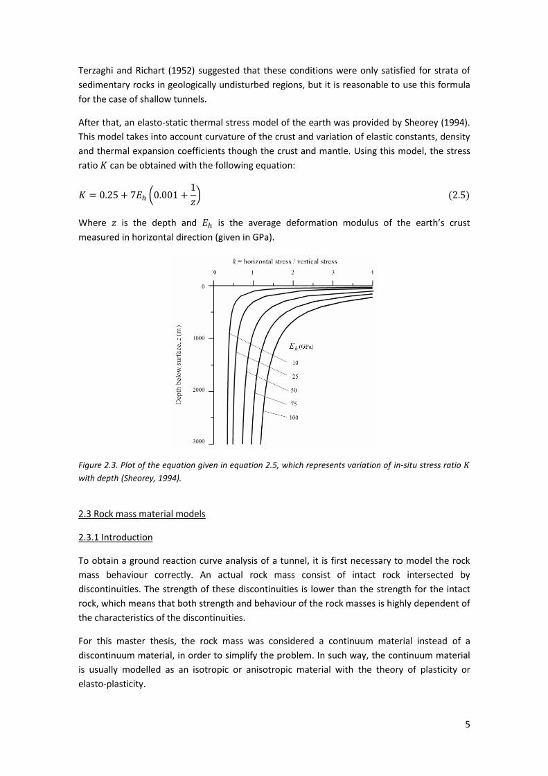
After that, an elasto-static thermal stress model of the earth was provided by Sheorey (1994).

This model takes into account curvature of the crust and variation of elastic constants, density

and thermal expansion coefficients though the crust and mantle. Using this model, the stress

ratio can be obtained with the following equation:

Where is the depth and is the average deformation modulus of the earth’s crust

measured in horizontal direction (given in GPa).

Figure 2.3. Plot of the equation given in equation 2.5, which represents variation of in-situ stress ratio

with depth (Sheorey, 1994).

2.3 Rock mass material models

2.3.1 Introduction

To obtain a ground reaction curve analysis of a tunnel, it is first necessary to model the rock

mass behaviour correctly. An actual rock mass consist of intact rock intersected by

discontinuities. The strength of these discontinuities is lower than the strength for the intact

rock, which means that both strength and behaviour of the rock masses is highly dependent of

the characteristics of the discontinuities.

For this master thesis, the rock mass was considered a continuum material instead of a

discontinuum material, in order to simplify the problem. In such way, the continuum material

is usually modelled as an isotropic or anisotropic material with the theory of plasticity or

elasto-plasticity.

6

To model the behaviour of continuum rock materials, it is needed to take into account the

constitutive relations between stresses and strains and a failure criterion which defines at

which stress level failure occurs. It is also important to have a basic knowledge about the

failure mechanisms which may appear in a tunnel. In the following subchapters, these aspects

mentioned above are described in further detail.

2.3.2 Material behaviour models

In rock mechanics, three main different material behaviour models can be found for

characterizing rock masses. The simplest one develops an elastic-perfectly plastic behaviour

(Fig. 2.4c). This means that when a specific value of the axial strain is achieved, is not possible

for the rock mass to come back to the previous strain level. In the second one, elastic-brittle

residual behaviour (Fig.2.4a) is assumed, which means that post peak dilatation occurs at a

constant rate with major principal strain in the residual plastic zone. The last one uses a tri-

linear elastic-strain softening-residual plastic stress-strain model (Fig.2.4b), with dilation

occurring at different rates with major principal stresses in the two different post peak zones.

(a) (b) (c)

Figure 2.4. Stress-strain behaviour models for: (a) Very good quality hard rock mass; (b) Average quality

rock mass; and (c) Very poor quality soft rock mass. (Hoek, 2001)

Despite the fact that it does not represent the stress-strain behaviour of the rock mass unless

the rock mass is of poor quality, elastic perfectly-plastic behaviour is the most commonly used.

In Fig. 2.5, it can be noticed that depending on the GSI value, one model or another can be

used to represent the rock mass behaviour properly. The drawback of the perfect-brittle and

strain-softening is mainly that it is more difficult to implement that kind of behaviour in the

analysis.

Figure 2.5. Different post-failure rock mass behaviour modes for rock masses with different geological

strength indices (GSI). Based on Hoek and Brown (1997).

7

2.3.3 Mohr-Coulomb failure criterion

The Mohr-Coulomb failure criterion is the most used criterion among continuum materials. It

is based on the work by Coulomb 1776 and Mohr 1882. In this criterion, it is assumed that the

shear stresses on any plane are limited by the condition:

Figure 2.6. Mohr-Coulomb failure criterion (Rock Mechanics Course, UPC).

Where is the shear stress at failure along the theoretical failure plane, is the cohesion, is

the normal effective stress acting on the failure plane and is the friction angle of the failure

plane.

The cohesion and friction angle (Mohr-Coulomb strength parameters) can be obtained from a

series of block shear test in exploration tunnels or from a number of triaxial tests. In this type

of tests, the minor and major principal stresses define a circle, and the tangential curve to

them creates the Mohr’s envelope. The Mohr-Coulomb failure criterion approximates this

envelope with a linear approximation.

2.3.4 Modelling a continuum material

A continuum material can be described according to the following relationship:

Where and are the stress and strain tensor respectively and is the elastic stress-

strain stiffness matrix. For an elastic material and plain strain conditions, the elastic stress-

strain stiffness matrix can be expressed as a function of elastic modulus and Poisson’s ratio

as follows:

Since stress-strain behaviour of rock masses is non-linear, the linear elastic model is not good

enough good to represent the actual behaviour. Because of that, is necessary to use the theory

of elasto-plasticity, which assumes that the strains in the rock mass can be divided into two

types of strain: elastic and plastic. This concept can be easily understood in the figure 2.7.

8

Figure 2.7. Total strains for an elasto-plastic material consisting of elastic and plastic strains (Johansson,

2006).

For each point of the stress-strain space, the total deformation can be expressed according to

equation 2.9.

Where is the increment of the total stress tensor and

and

are the increments of

the elastic and plastic strain tensors respectively. The relationship between elasto-plastic

strain and stress increments is represented as equation 2.10.

Where is the elasto-plastic stress-strain matrix and is the increment of the stress

tensor.

In order to calculate the plastic deformations

, the following concepts are necessary:

A yield criterion.

A flow rule.

A hardening rule.

Yield criterion

The yield or failure criterion defines the limit between plastic and elastic deformations as a

function of the principal stress state. The yield criterion is usually expressed as:

Where is the hardening parameter which controls the size of the yield surface. There are

some particular cases which are worth to mention regarding the value of the yield surface, and

they are also depicted in figure 2.8.

9

Figure 2.8. Location of the yield and failure surface in the principal stress space (Johansson, 2005).

Flow rule

The flow rule gives the relationship between the different components of the incremental

plastic deformation. The plastic flow at yield is assumed to be governed by the so-called plastic

potential function expressed in equation 2.12.

It is well known from the theory of plasticity that the plastic strains are determined by:

Where is a constant called the plastic multiplier which can be derived from stress strain

curves obtained from triaxial tests. The value of represents the magnitude of the plastic

deformation and the direction is given by the gradient of . The direction of the plastic

deformation is parallel to the gradient of ; therefore, the direction of the plastic deformation

is always perpendicular to the surfaces that obey that is a constant value.

When the yield criterion equals the plastic potential, in other words when

, the flow rule is said to be associated. Otherwise, the flow rule is non-associated.

Hardening rule

The hardening rule expresses the variation of size, shape and position of the yield surface. This

concept can also be understood as a resistance against plastic deformations. The hardening

modulus can be expressed as follows:

Where greater than zero characterizes hardening, lower than zero characterizes softening

and equal to zero means that it is a perfectly plastic material.

10

Calculation of the total deformation

With all the three concepts explained above, and the consistency condition, the plastic part of

the elasto-plastic stress-strain stiffness matrix can be derived. The consistency condition

implies that the stresses must be on the yield surface while plastic loading occurs. Equation

2.15 represents the consistency equation:

Operating and using the equations deduced in this subchapter, we can obtain the final

expression between strains and stresses:

2.3.5 Failure modes in tunnels

Effective ground support takes into account the mode of instability so that the support

components can be designed to work efficiently for the anticipated instability mode. There are

three main tunnel instability mechanisms (Aydan et al,1993):

Rock mass shear yielding, which is quite common in poor quality rock masses. A plastic

zone is formed around the tunnel and, depending upon the ratio of rock mass strength to

in-situ stress, this may stabilize, or it may continue to expand until the tunnel collapses.

The two main mechanisms that can produce this type of instability are swelling or

squeezing conditions.

Figure 2.9. Shear failure occurs in a plastic zone around tunnels in weak rock (Hoek, 2008).

Structurally controlled kinematic instability, which appears in jointed rock masses under

low in-situ stress conditions. Gravity driven wedge instability is typically the dominant

instability mode. This type of failure involves gravity falls of wedges defined by intersecting

geological features.

11

Figure 2.10. Gravity driven wedge instability along pre-existing geological structures dominates in

blocky ground under low in-situ stress conditions (Hoek, 2008).

Brittle rock failure, which initiates as a result of the propagation of tensile cracks from

defects in highly stressed massive hard rock. These cracks generally propagate along the

maximum principal stress trajectories, resulting in thin splinters or slabs. Depending upon

the ratio of intact rock strength to in-situ stress, spalling may be limited to small plate-

sized slabs, or it may develop into a massive violent failure or rockburst.

Figure 2.11. Stress driven brittle failure tends to dominate in massive brittle rock under high in-situ

stress conditions (Hoek, 2008).

However, in many cases, more than one of the potential failure modes is possible for a tunnel.

For conditions where no experience is available, the dominant mode of failure may not be

known. Furthermore, it is not always clear when this transition between failure modes will

occur or how the rock mass will behave during the transition. There is currently no general

analysis methodology for transitional behaviour. Therefore, it is recommended that all

potential modes of failure be analyzed for transitional cases.

12

2.4 Shallow tunnels vs. deep tunnels

The aim of this master thesis is to analyze the limitations of the ground reaction curve for

shallow tunnels. Shallow tunnels are the most extended ones within civil engineering projects

and deep tunnels are usually found in mining industry. In shallow tunnels, it is not in general

advisable to assume isotropic stress field conditions, so a differentiation between these two

types of tunnels has to be made.

In shallow tunnels, the proximity of the ground surface usually means that the preferred

failure path for the rock mass surrounding the tunnel and ahead of the face is to “cave” to the

surface. Because of the different failure processes, convergence confinement method cannot

be applied directly to this problem. Traditional approaches for tunnels at shallow depth usually

involve the assumption that the rock load is calculated on the basis of the dead weight of the

rock mass above the tunnel.

Near the surface, rock masses are subject to stress relief, weathering and blast damage as a

result of nearby excavations. These processes disrupt or destroy the interlocking between rock

particles that play an important role in determining the overall strength and deformation

characteristics of rock masses.

Regarding rock support, much work has been done within the civil engineering industry. For

civil tunnels, support typically consists of installing initial support (shotcrete and rockbolts)

followed by a final liner (precast concrete segments with a water seal). Initial support typically

is designed for the construction period and must provide a safe working environment and

support excavation-induced loading over a relatively short time period. The final liner typically

is designed with a suitably conservative factor of safety (FS) and is required to maintain long-

term loading conditions. Geometrically, compared to civil tunnels, mining tunnels are often

small and in close proximity to other excavations.

Figure 2.12. The excavation-induced stresses reach a maximum (approximate) distance three tunnel

diameters behind the tunnel face (X/D > 3). However, mining tunnels can experience significantly greater

mining-induced stresses (and displacements). (Report from Itasca, 2010).

13

2.5. Calculation methods

2.5.1 Introduction

In general, two different types of methods are used in order to calculate the ground reaction

curve of a tunnel. One of them is the analytical methods, which are expressed in mathematical

terms. The other calculation method is the numerical methods, where the differential

equations of the problem are solved numerically.

2.5.2 Analytical method: Convergence confinement method

The Convergence confinement method (CCM) has been described by some authors (e. g.,

Gesta et al., 1980; Fairhurst and Carranza-Torres, 2002) and has been commonly used for the

support system design in conventional tunnelling; achieving 2D simplified approach for

resolving 3D rock-support interaction problems.

The main assumption of the CCM is that the support load required to stabilize the excavation

decreases with inward tunnel displacement. As the boundary rock moves inward, tangential

stresses increase, which results in both yielding of the rock mass and increased confining

stresses on the surroundings (contribute to stabilize). The CCM is comprised by three basic

elements: the ground reaction curve (GRC), the longitudinal deformation profile (LDP) and the

support characteristic curve (SCC).

The Support Characteristic Curve (SCC) concept was firstly presented by Hoek and Brown

(1980) and it is defined as a graphical representation of the pressure of the rock support for

different radial deformations of that support. The most common means of support are bolts

(grouted or steel-made) and shotcrete.

The Ground Reaction Curve (GRC) can be defined as a curve that describes the decreasing of

inner pressure and the increasing of radial displacement of tunnel wall. The fundamental

concept of this method is that the intersection between the GRC and the SCC gives the

pressure and tunnel deformation at the equilibrium point. Because of that, the determination

of these two lines is a key aspect in designing tunnel support.

The Longitudinal Deformation Profile is a graphical representation of the radial displacement

that occurs along the axis of an unsupported excavation, for sections located ahead of and

behind the face. The horizontal axis represents the distance from the section analyzed to the

tunnel face, while the vertical axis represents the corresponding radial displacement. (Zhang et

al., 2008).

The main advantage of the CCM, as mentioned previously, is that three dimensional tunnel

advance can be captured in two dimensions by relating distance from tunnel face in the LDP to

inner pressure in the GRC. Moreover, a factor of safety can be calculated by comparing the

support capacity with the load demand. CCM calculations can be carried out using closed-form

solutions, numerical models, or some combination of each to develop the required curves. The

method is illustrated in Figure 2.13.

14

Figure 2.13. Schematic representation of the relation between LDP, GRC and SCC for use in the Convergence Confinement Method (Fairhurst and Carranza-Torres, 2002).

This method assumes that the support elements act as equivalent uniform support pressure acting over the tunnel contour, and that the reinforcement and support do not significantly affect the displacement characteristics of the tunnel prior to achieving a stable state.

2.5.3 Ground reaction curve as a part of the CCM

Elastic range

The gradual unloading of isotropic and homogeneous rock mass, with hydrostatic in-situ stress

surrounding a circular tunnel can be treated as an axisymmetrical cavity problem in infinite

space. Because of the axial symmetry of the problem, the tangential and radial stresses

are major and minor principal stresses, and , respectively.

The first authors that stated the concept of the ground reaction curve were Hoek, Brown, Bray

and Ladanyi in 1980. The solutions for a circular tunnel in an infinite medium under hydrostatic

initial ground pressure presented in this chapter were developed by Stille (1983, 1989).To

solve this problem, an elasto-plastic rock mass with the Mohr-Coulomb’s failure criterion and a

non-associated flow rule for the dilatancy after failure are assumed (dilatancy angle is equal to

0). Equilibrium, compatibility and strain stress relationship equations are needed to obtain the

final formulation of the ground reaction curve.

15

Figure 2.14. Acting forces around a circular opening in a differential element (Rock Mechanics Course,

KTH).

The starting point to get the ground reaction curve solution is the equilibrium condition:

The following compatibility conditions must be fulfilled:

By theory, we know that the stress-strain relationships can be expressed as follows:

16

Where is the Young’s Modulus of rock mass and is the Poisson’s ratio of rock mass.

As plain strain conditions are assumed, the value of is set to zero. After that, rearranging the

previous equations we get:

Where:

Using Eq. 2.22 and 2.23 into Eq. 2.28 and 2.29, the next differential equation is obtained:

Applying the boundary conditions below:

Where is the internal pressure, is the initial in-situ stress value and is the tunnel

radius.

The stresses and deformation in the elastic zone can be determined by the following

equations:

Plastic range

In the plastic zone near to the tunnel surface, the following stresses will develop:

17

Where

Where is the value for cohesion and is the value for friction angle.

To calculate , which the radius of plastic zone is, the following expression must be used:

Notice that plastic flow begins when , so:

Finally, the deformation of the tunnel surface is given by:

Where is a factor which describes the volume expansion after failure and is given by

equation 2.41.

Where is the dilatancy angle.

2.5.4 Numerical methods

The numerical methods for rock mechanics problems are divided into two main groups, the

continuum methods and the discontinuous methods. The scale of the problem and the

geometry of the joint system are the main factors to decide which of those models that has to

be used.

For the continuum methods, there exist three main approaches: the Finite Difference Method

(FDM), the Finite Element Method (FEM) and the Boundary Element Method (EM). The

difference between them is the solution technique to solve the Partial Differential Equations

system of the problem.

18

For the discontinuous methods, Distinct Element Method (DEM) (Cundall, 1980), and the

Discontinuous Displacement Analysis (DDA) are the main ones. These methods enable large

displacements of separate intact blocks, and can model rotation and translation of the blocks.

It is important to be aware that the weak point of the analytical methods is that they cannot

represent complex in-situ conditions and geometry, which are the main reasons for using

numerical methods. The numerical methods should be used carefully and with a complete

understanding of the background of the problem which is being analyzed, in order to get the

right conclusions.

2.6 Practical applications of the approach

2.6.1 Limitations

In spite of having a quite good acceptance and its frequent use, the analytical solution of the

ground reaction curve has some drawbacks that limit its usage. The main disadvantages stem

from the assumptions that have to be made. These are: (1) circular cross section of the tunnel,

(2) homogeneous rock mass around the tunnel, (3) isotropic stress field, (4) plain strain

conditions (or very long tunnel), (5) and gravity force is neglected.

2.6.2 Tunnel with non-circular section and anisotropic initial stress field

In general, because these assumptions are usually violated in practical tunnelling conditions,

“The ground reaction curve family concept” was introduced by Pan and Chen (1990). The main

aim of these authors was to have a deeper understanding about how the internal pressure and

deformation of the tunnel varied at various points on the tunnel wall depending on the initial

stress conditions and the tunnel shape.

In order to obtain that ground reaction curve families, a numerical analysis by the finite

element method was performed. These numerical solutions were obtained considering elasto-

plastic conditions on the one hand, and Mohr-Coulomb failure criterion on the other hand.

The ground reaction curve families are depicted in Figures 2.15 to 2.17 for different tunnel

shapes and different initial stress ratio (horizontal stress over vertical stress). In these

graphs, the normalized stress is represented in the vertical axis and the normalized

deformation is represented in the horizontal axis.

19

Figure 2.15. Ground Reaction Curve families for a circular tunnel when initial stress ratio equals to (A)

1.0, (B) 1.5, and (C) 2.0 (Pan and Chen, 1990).

20

Figure 2.16. Ground Reaction Curve families for an elliptical tunnel when initial stress ratio equals to (A)

0.75, (B) 1.0, and (C) 1.5 (Pan and Chen, 1990).

21

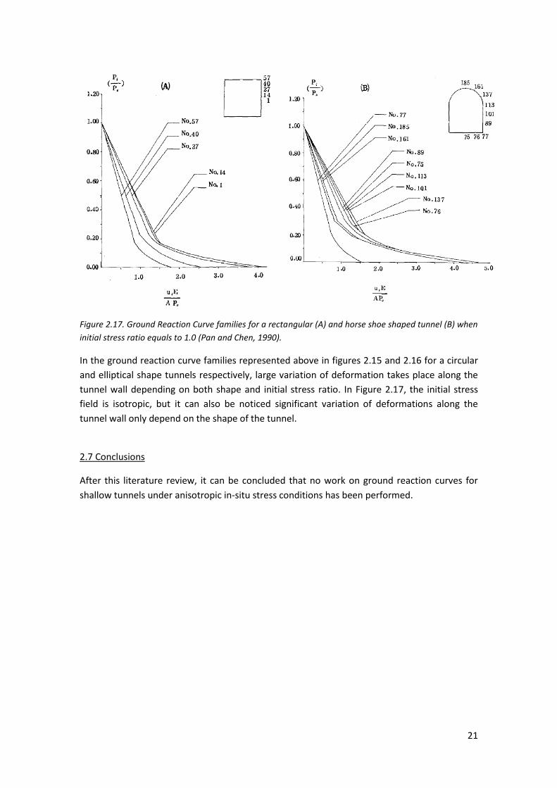
Figure 2.17. Ground Reaction Curve families for a rectangular (A) and horse shoe shaped tunnel (B) when

initial stress ratio equals to 1.0 (Pan and Chen, 1990).

In the ground reaction curve families represented above in figures 2.15 and 2.16 for a circular

and elliptical shape tunnels respectively, large variation of deformation takes place along the

tunnel wall depending on both shape and initial stress ratio. In Figure 2.17, the initial stress

field is isotropic, but it can also be noticed significant variation of deformations along the

tunnel wall only depend on the shape of the tunnel.

2.7 Conclusions

After this literature review, it can be concluded that no work on ground reaction curves for

shallow tunnels under anisotropic in-situ stress conditions has been performed.

22

3. METHODOLOGY

3.1 Introduction

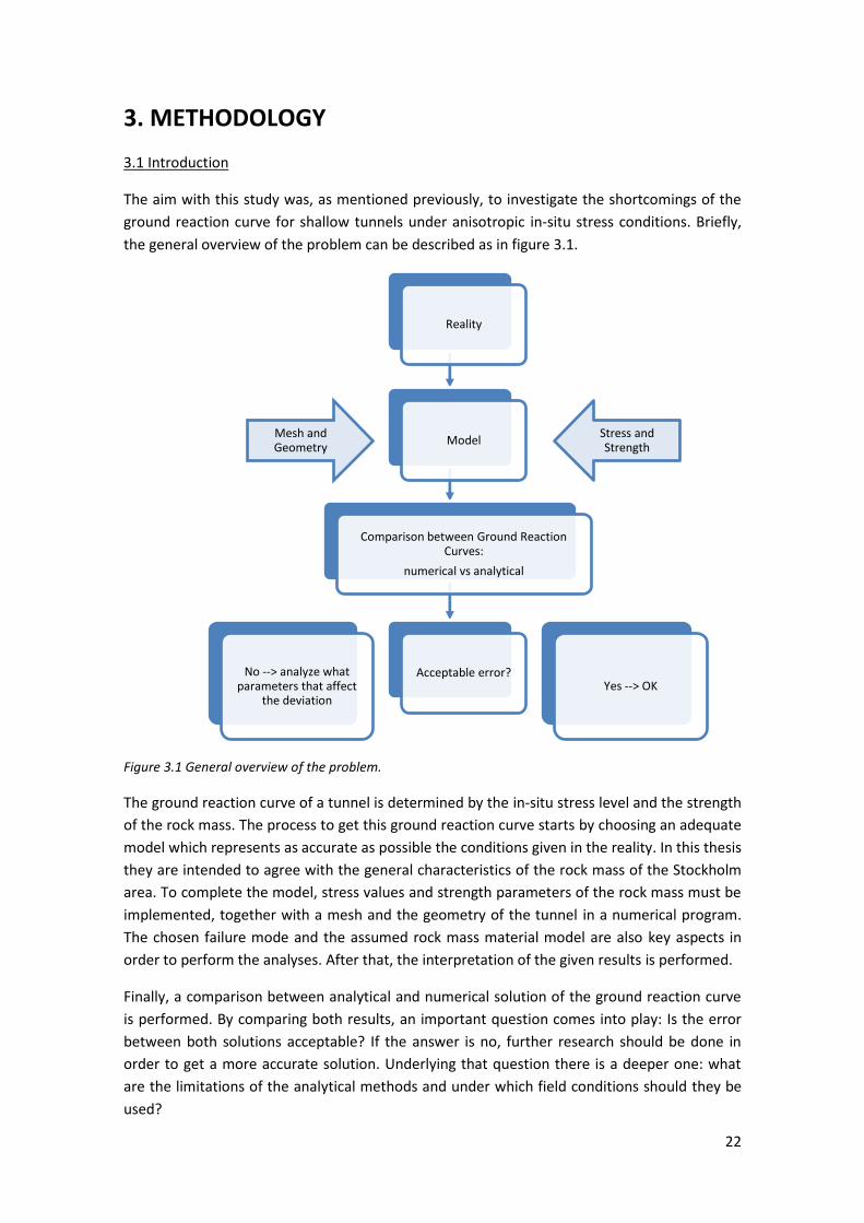
The aim with this study was, as mentioned previously, to investigate the shortcomings of the

ground reaction curve for shallow tunnels under anisotropic in-situ stress conditions. Briefly,

the general overview of the problem can be described as in figure 3.1.

Figure 3.1 General overview of the problem.

The ground reaction curve of a tunnel is determined by the in-situ stress level and the strength

of the rock mass. The process to get this ground reaction curve starts by choosing an adequate

model which represents as accurate as possible the conditions given in the reality. In this thesis

they are intended to agree with the general characteristics of the rock mass of the Stockholm

area. To complete the model, stress values and strength parameters of the rock mass must be

implemented, together with a mesh and the geometry of the tunnel in a numerical program.

The chosen failure mode and the assumed rock mass material model are also key aspects in

order to perform the analyses. After that, the interpretation of the given results is performed.

Finally, a comparison between analytical and numerical solution of the ground reaction curve

is performed. By comparing both results, an important question comes into play: Is the error

between both solutions acceptable? If the answer is no, further research should be done in

order to get a more accurate solution. Underlying that question there is a deeper one: what

are the limitations of the analytical methods and under which field conditions should they be

used?

Reality

Mesh and Geometry

Model

Comparison between Ground Reaction Curves:

numerical vs analytical

No --> analyze what parameters that affect

the deviation

Acceptable error? Yes --> OK

Stress and Strength

23

The numerical analysis has been carried out by UDEC 5.0 (Itasca,2010), which is the acronym

of Universal Distinct Element Code. It is a two dimensional numerical program based on the

distinct element method. UDEC is based on a “Lagrangian” calculation scheme that is well-

suited to model the large movements and deformations of a blocky system.

3.2 Overview and general features of UDEC 5.0

UDEC was firstly presented by Cundall in 1971, and has continuously been updated till the

latest version 5.0, which was released last year. After that, Dr. Cundall and Itasca staff adapted

UDEC to perform engineering calculations on a microcomputer.

The term “distinct element method” was used for the first time by Cundall and Strack (1979) to

refer to the particular discrete element scheme that uses deformable contacts and an explicit

time-domain solution of the original equations of motion.

UDEC has been developed with the purpose of solving a widespread range of rock engineering

problems, from evaluations of rock slope failure to behaviour analyses of rock joints and faults

on underground excavations.

Blocks in UDEC can be either rigid or deformable. There are seven built-in material models for

deformable blocks, ranging from the “null” block material (excavations) to the shear and

volumetric yielding models.

In UDEC, a two-dimensional plain-strain state is assumed. This condition appears for long

structures or excavations with constant cross-section acted on by loads in the plane of the

cross section. Because of this assumption, discontinuities are considered to be oriented normal

to the plane of the cross section.

Other features about UDEC are that it is able to carry on either static or dynamic analysis; it

permits to simulate flow trough discontinuities; it includes structural elements to simulate rock

reinforcement and surface support; it has a thermal mode available; and it is comprised by a

programming language called FISH, which enables the user to define new variables and

functions.

3.3 Input to the model

Introduction

The models explained in the previous subchapter contained the specification or execution of

the following parts:

Idealization of the tunnel into a two dimensional problem.

Input of tunnel geometry.

Input of the rock mass geometry.

Specification of boundary conditions.

24

Material model and properties for the rock mass.

Generation of in-situ stress condition.

Discretisation of the model into finite element.

Figure 3.2. Definition of depth and stress distribution into the model.

In figure 3.2, the distribution of stresses that affect the rock mass is represented. It can be

noticed also that the depth is defined as the distance from the ground surface to the centre

of the tunnel.

To show how the finite element models were constructed, and which assumptions and

material properties that were used in the analysis, each step above is described in the

following text.

Idealization into a two dimensional problem

The real three dimensional problem can be idealized in a two dimensional problem where

plain strain conditions are assumed. To obtain accurate numerical results assuming plane

strain conditions, the following assumptions have to be fulfilled:

There is no curvature along the transversal axis of the tunnel.

The rock cover above the tunnel does not vary along the transversal axis of the tunnel.

There are no fractures or fault planes around the tunnel that might affect stress

redistribution or deformations.

In practice, these conditions are sometimes fulfilled, but in general they are not. This means

that the analytical solution is not always strictly valid for field conditions. Therefore, in the case

that the analytical solution is used, we must be aware about the in-situ rock mass conditions

and judge by ourselves if it is fair to assume these conditions or not.

Tunnel geometry

The shape of the cross section of the tunnel is circular and the input diameter was 5 meters.

The analysis for the ground reaction curves was only performed for a circular tunnel because

one of the requirements of the analytical solution is that the cross section of the tunnel has to

be circular.

25

Rock mass geometry

In order to define the geometry of the model into UDEC 5.0 it is necessary to define the level

of the rock mass surface for each depth. The constant values are the level of the bottom,

which is -25 meters and the width of the block, which is 50 meters.

As can be noticed, the model of the rock mass is rectangular and is assumed to be continuum

and homogeneous material, without fractures or fault planes.

Boundary conditions

For the vertical boundaries, it was assumed that the rock mass is restricted to move in the

vertical direction. At the lower horizontal boundary it was assumed that the rock mass is free

to move in the horizontal direction. No movement restrictions were assumed for the top

boundary, which means that it is free to move in whatever direction.

Rock mass material model

The rock mass was modelled with the Mohr-Coulomb constitutive model, which means that

plastic behaviour may appear in the rock mass.

The following values of the input parameters, were used:

Density of the rock mass:

Young Modulus of the rock mass:

Poisson ratio:

Cohesion of the rock mass:

Friction angle of the rock mass:

Dilation angle:

Tensile strength of the rock mass:

The parameters have been assumed in order to represent a good quality of the rock mass with

GSI values in the range of 50-70.

Generation of in-situ stress conditions

The in-situ stress was generated assuming that the vertical total stresses are the result of the

dead weight of the rock mass and the horizontal total stresses are the prescribed values

explained before for each load case.

The vertical total stress is given by equation 3.1:

Where is the specific weight of the material and is the depth from the rock mass surface. In

the calculations, the density for the rock mass was set to 2700 kg/m3 and the gravity was set to

10 m/s2.

26

The initial stress ratio , as mentioned before, was a prescribed value for each case.

Therefore, the value of the horizontal stress was calculated as the vertical stress multiplied

by the value.

To represent actual conditions as close as possible, a linear varying initial stress was set by the

gradient command. No gradient was assumed in x axis. A linear variation was implemented in y

axis for both horizontal and vertical stresses. In the z axis, a linear variation was assumed for

the horizontal and vertical stresses as well.

Discretisation of the model into “distinct elements”

The division of the model into a number of “distinct elements” was performed using the

automatic mesh generator in UDEC.

Numerical error of the results varies depending on the type of chosen mesh elements, its size

and its aspect ratio. In order to optimize the calculation time that UDEC needs to yield the

results, a sensitivity analysis was performed. This analysis consisted in calculate the mesh size

element that provided accurate results. These results were assumed to be accurate enough

when for the two different mesh sizes, they differed less than 2%.

Datafiles

The model was ran with the command solve relax, which is used to slowly reduce the forces on

the inside of an excavation in order to avoid a large tensile stress wave. This tensile stress

wave may cause dynamic failure in zones that would not normally fail under the static stresses

caused by the excavation.

In order to make sure that equilibrium has been reached, a quick check was done by plotting

the change in maximum unbalanced force for each time step.

Regarding the boundary conditions, fixed rolled boundary conditions were supposed in the

bottom and in both sides’ of the rock mass. No boundary conditions were applied at the top

boundary. To implement these conditions in UDEC, the movement in x direction was disabled

in both left and right boundaries; and for the bottom boundary, movement in y axis was

disabled.

3.4 Quality check of the model

Before the simulations started, a crucial step was to check how the analytical formulation

deviates from the numerical one under ideal conditions. The aim of this was to be sure that

the input data in the model was correct.

To do that, a simplified model was implemented in UDEC. The geometry of the block mass was

circular, since the results are more accurate with this kind of geometry. The characteristics of

the rock mass were the same that were mention in subchapter 3.4. The tunnel was modelled

as a circular section of 5 meters diameter.

27

The results of the quality check were satisfactory, the numerical solution deviated less than 4%

for all the cases analyzed for this section, where different in-situ stresses were assumed.

3.5 Obtaining the ground reaction curves

In order to determine under which conditions the analytical solution of the ground reaction

curve should be used, ten different load cases were analyzed for each depth. All of those cases

are calculated by both numerical and analytical methods. The depths that were used in the

analysis were tunnel covers of 2,5; 5; 10; 15 and 20 meters (or tunnel depths of 5; 7,5; 15,5;

17,5 and 22,5 meters).

Ten different load cases were implemented. For all those ten different load cases, the vertical

stress value is given by the dead weight of the rock mass above the point situated at the depth

of the centre of the tunnel, assumption that is not far from the reality. Regarding to the

horizontal stresses, they vary from one case to another and their values are obtained using the

initial stress ratio . The analyzed cases are for values of 1, 2, 3, 4, 5, 6, 7, 8, 9 and 10.

3.6 Obtaining an empirical equation

In order to get the final displacement of the wall and the crown for shallow tunnels, some

empirical equations were derived. Also, an attempt to get an empirical formula for the ground

surface displacements was done. These formulae are based on numerical results given by

UDEC.

First of all, it is important to be aware that the rock mass conditions assumed in this thesis are

rather good. This means that is difficult to have plastic behaviour of the rock mass, so the

formulae work quite well for elastic conditions in shallow tunnels.

In order to get those empirical equations, almost 400 different simulations were performed. In

the simulations, the parameters that varied from one model to another were: the radius of the

tunnel, the Young’s modulus of the rock mass and the Poisson’s ratio. The reason of choosing

these parameters is because they are the ones that affect the displacement under elastic

conditions. Apart from those rocks material parameters, the models were also ran for different

depths of the tunnel and different initial stress values .

The method used to get the empirical formulae was the “multiple linear regression method”,

which is explained in further detail in Appendix A. In appendix B, there are some plots of the

models performed for this analysis together with a brief explanation of the procedure to get

those displacements from UDEC 5.0. The results from the multiple linear regression are in

appendix C.

28

3.7 Presentation of data

UDEC is able to plot a wide variety of graphs as well as numerical data, such as in-situ stresses,

displacement magnitudes, displacement velocities, zones with plastic failure, etc. Because of

that, a filtering of all that information was done, and a subjective decision about which plots

should be shown and analyzed has to be taken.

From an engineering point of view, the most important parameters that have to be analyzed

are stresses in the surroundings of the excavation and the displacements of the crown and

walls of the tunnel, which may produce subsidence or heaving in the ground surface because

we are dealing with shallow tunnels. Since heaving may also occur in these cases, the

displacements of the ground surface were also checked.

Apart from that, the ground reaction curves will be shown in chapter 4, together with the ones

that were calculated with the analytical formulation.

29

4. RESULTS

4.1 Presentation of the results

In total, 50 models were run in UDEC in order to calculate the ground reaction curves for

different depths and also different initial stress ratios. These 50 models covered 5 different

depths: 5; 7,5; 12,5; 17,5 and 22,5 meters from the surface to the centre of the tunnel and

covered also initial stress ratios from 1 to 10. These models were performed for a circular

cross-section of 5 meters diameter.

4.2 Ground reaction curves

4.2.1 Introduction

In this subchapter, the ground reaction curves for the shallower tunnel (5 meters depth) and

the deep tunnel (22,5 meters depth) for the initial in-situ stress values 1,2,4 and 6 together

with some comments will be plotted. The rest of the ground reaction curves can be found on

appendix E, where they are represented into groups with respect to depth.

The plots have been performed with the help of excel by including the values yielded by the

numerical analyses. In appendix D, several plots of these analyses can be found. The plots

included in that appendix correspond to displacement vectors, displacement magnitudes,

major and minor principal stresses. In addition, plots of tensile and plastic failure are

presented.

In every graph, there are 4 ground reaction curves, which correspond for the analytical

solution. One for a point in the wall of the tunnel, one for a point in the crown of the tunnel

and one for a point in the floor of the tunnel.

The analytical ground reaction curves turn out to be straight lines for every single case. The

reason is that the rock mass are in elastic range for all the analysed cases.

4.2.2 Ground reaction curves for tunnel depth of 5 meters

In figure 4.1, it can be noticed that the GRC for the point on the wall agrees rather well with

the one obtained with analytical formulation. However, in the case of the points on the crown

and on the floor, the influence of the shallow depth makes the ground reaction curve to

deviate from the analytical values.

30

Figure 4.1 Ground reaction curve for =1 and tunnel depth of 5 meters.

Figure 4.2 shows that the deviation between the GRC of the wall and the analytical is

becoming higher. At the same time, the GRC of the crown and floor move back to the left

because of the influence of the horizontal stresses, achieving negative displacements in the

case of the crown.

Figure 4.2 Ground reaction curve for =2 and tunnel depth of 5 meters.

0

0,1

0,2

0,3

0,4

0,5

0,6

0,7

0,8

0,9

1

0 0,01 0,02 0,03 0,04 0,05

Analytical

Wall

Crown

Floor

0

0,1

0,2

0,3

0,4

0,5

0,6

0,7

0,8

0,9

1

-0,02 0 0,02 0,04 0,06 0,08

Analytical

Wall

Crown

Floor

31

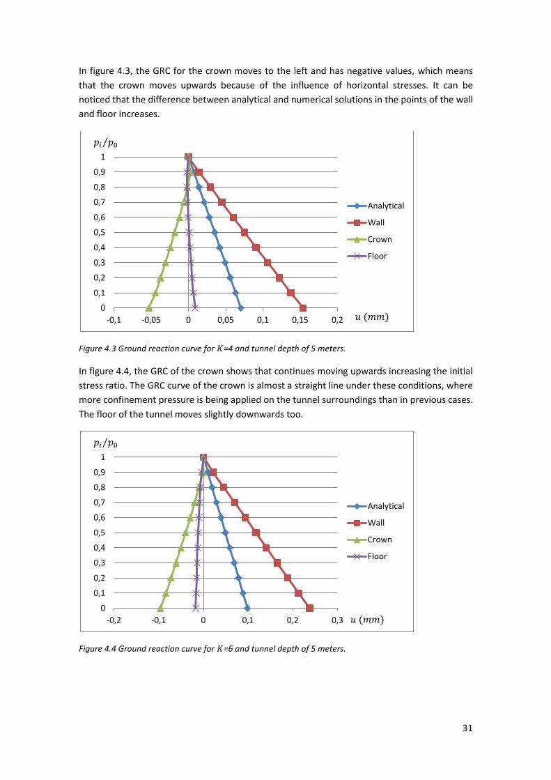
In figure 4.3, the GRC for the crown moves to the left and has negative values, which means

that the crown moves upwards because of the influence of horizontal stresses. It can be

noticed that the difference between analytical and numerical solutions in the points of the wall

and floor increases.

Figure 4.3 Ground reaction curve for =4 and tunnel depth of 5 meters.

In figure 4.4, the GRC of the crown shows that continues moving upwards increasing the initial

stress ratio. The GRC curve of the crown is almost a straight line under these conditions, where

more confinement pressure is being applied on the tunnel surroundings than in previous cases.

The floor of the tunnel moves slightly downwards too.

Figure 4.4 Ground reaction curve for =6 and tunnel depth of 5 meters.

0

0,1

0,2

0,3

0,4

0,5

0,6

0,7

0,8

0,9

1

-0,1 -0,05 0 0,05 0,1 0,15 0,2

Analytical

Wall

Crown

Floor

0

0,1

0,2

0,3

0,4

0,5

0,6

0,7

0,8

0,9

1

-0,2 -0,1 0 0,1 0,2 0,3

Analytical

Wall

Crown

Floor

32

4.2.3 Ground reaction curves for tunnel depth of 22,5 meters

In figure 4.5 can be observed that the GRC of the crown and bottom is not as curved as in the

first case for a very shallow depth. The analytical solution and the numerical one agree almost

perfectly for the wall displacement.

Figure 4.5 Ground reaction curve for =1 and tunnel depth of 22,5 meters.

Figure 4.6 shows that the deviation between the GRC of the wall, floor and crown and the

analytical ones is becoming higher.

Figure 4.6 Ground reaction curve for =2 and tunnel depth of 22,5 meters.

In figures 4.7 and 4.8, the trend is the same. They deviate more and more when the initial in-

situ stress ratio increases.

0

0,1

0,2

0,3

0,4

0,5

0,6

0,7

0,8

0,9

1

0 0,05 0,1 0,15

Analytical

Wall

Crown

Floor

0

0,1

0,2

0,3

0,4

0,5

0,6

0,7

0,8

0,9

1

0 0,1 0,2 0,3 0,4

Analytical

Wall

Crown

Floor

33

Figure 4.7 Ground reaction curve for =4 and tunnel depth of 22,5 meters.

Figure 4.8 Ground reaction curve for =6 and tunnel depth of 22,5 meters.

4.3 Limitations of the ground reaction curve concept

4.3.1 Introduction

The main purpose of this work was to study the limitations of the ground reaction curve

concept for shallow tunnels. In order to do so, a comparison between the analytical solution

and the one given by UDEC was done, taking into account the initial stress ratio and the

depth of the tunnel. The comparison between both solutions is expressed as the ratio between

the numerical solution over the analytical solution.

0

0,1

0,2

0,3

0,4

0,5

0,6

0,7

0,8

0,9

1

-0,2 0 0,2 0,4 0,6 0,8

Analytical

Wall

Crown

Floor

0

0,1

0,2

0,3

0,4

0,5

0,6

0,7

0,8

0,9

1

-0,5 0 0,5 1 1,5

Analytical

Wall

Crown

Floor

34

4.3.2 Limitations for the tunnel wall

Figure 4.9 represents how the numerical result deviates from the analytical one when

increasing the initial stress ratio for fixed values of the depth. The UDEC/Analytical ratio is

named as from now on. This graph indicates clearly that the analytical solution and the

numerical one agree almost perfectly for isotropic conditions, even for very shallow tunnels

where . However, if this initial stress value increases, the analytical solution does not

achieve good results.

Figure 4.9 UDEC/Analytical ratio plotted against initial stress ratio , differentiated by groups of depth

for the tunnel wall.

In figure 4.10, on the other hand, slight changes can be seen from one case to another when

increasing the depth. This means that the in-situ stress factor is a much heavier component of

the final displacement than the depth. For isotropic stress field, the analytical solution and the

numerical one agree perfectly, independently of the depth.

Figure 4.10 UDEC/Analytical ratio plotted against depth, differentiated by groups of initial stress ratios

for the tunnel wall.

0,5

1

1,5

2

2,5

0 2 4 6 8

Depth 5

Depth 7,5

Depth 12,5

Depth 17,5

Depth 22,5

0,5

1

1,5

2

2,5

0 5 10 15 20 25

K = 1

K = 2

K = 4

K = 6

35

4.3.3 Limitations for the tunnel crown

Figure 4.11 shows that the displacements of the crown do not agree as good as the

displacements of the wall for isotropic conditions. This happens because the tunnel depth has

more influence in the crown displacement than in the wall displacement.

It can also be noticed also that for initial stress ratios higher than a value between 2 and 4

depending on the depth, the displacements of the crown turn out to be negative. This means

that the crown moves upwards instead of moving downwards, because the confinement

pressure in the horizontal direction is higher enough to cause this behaviour.

Figure 4.11 UDEC/Analytical ratio plotted against initial stress ratio , differentiated by groups of depth

for the tunnel crown.

Figure 4.12 shows that the depth influences the displacements of the crown more than the

displacements of the wall. For isotropic conditions and for high values of the depth, the

analytical solution and the numerical one tend to agree. However, for initial stress ratios

higher than 1, both solutions tend to deviate more and more. It is important to notice that the

displacements calculated by the analytical formulation under isotropic stress field are always

overestimated ( values lower than one).

Figure 4.12 UDEC/Analytical ratio plotted against depth, differentiated by groups of initial stress ratios

for the tunnel crown.

-1,5

-1

-0,5

0

0,5

1

0 2 4 6 8

Depth 5

Depth 7,5

Depth 12,5

Depth 17,5

Depth 22,5

-1,5

-1

-0,5

0

0,5

1

0 5 10 15 20 25

K = 1

K = 2

K = 4

K = 6

36

4.3.4 Limitations for the tunnel floor

In figure 4.13, it can be noticed that the displacements of the floor do not agree as good as the

displacements of the wall for isotropic conditions. The shape of the curve is similar to the one

for the crown. As for the crown, the tunnel depth has more influence in the floor displacement

than in the wall displacement. It can also be noticed also that for initial stress ratios around 4,

the factor tends to 0, which means that the displacements in the floor approach to 0 at that

confinement levels. For shallow depths and high initial stress ratios, the displacements of the

floor turn out to be negative (the floor moves downwards).

Figure 4.13 UDEC/Analytical ratio plotted against initial stress ratio , differentiated by groups of depth

for the tunnel floor.

Figure 4.14 shows that the depth influences the displacements of the floor more than for the

displacements of the wall. For isotropic conditions and for high values of the depth, the

analytical solution and the numerical one tend to agree. However, for initial stress ratios

higher than 1, both solutions tend to deviate more and more.

Figure 4.14 UDEC/Analytical ratio plotted against depth, differentiated by groups of initial stress ratios

for the tunnel floor.

-0,5

0

0,5

1

1,5

2

0 2 4 6 8

Depth 5,0

Depth 7,5

Depth 12,5

Depth 17,5

Depth 22,5

-0,5

0

0,5

1

1,5

2

0 5 10 15 20 25

K = 1

K = 2

K = 4

K = 6

37

4.3.5 Limitations under isotropic stress field conditions

The plots of the UDEC/Analytical ratio against depth under isotropic conditions are

represented in figure 4.15 for the tunnel wall, crown and floor. It can be appreciated that the

deviation of the displacement of the tunnel wall from the analytical solution is independent of

the depth (the numerical solution always agrees with the analytical one).

The UDEC/Analytical ratio for the crown is below 1, which means that the analytical solution

overestimates the displacements in this case. The ratio becomes 1,00 for a depth of 37,5

meters approximately in the case of the crown .

On the other hand, the UDEC/Analytical ratio for the tunnel floor is above 1, which means that

the analytical solution underestimates the displacements in this case. The ratio becomes

1,00 for a depth of 32,5 meters approximately in the case of the tunnel floor .

Figure 4.15 UDEC/Analytical ratio plotted against depth for isotropic stress field conditions.

4.3.6 Limitations for a “deep” tunnel

The plots of the UDEC/Analytical ratio against initial in-situ stresses are represented in figure

4.16 for a “deep” tunnel. The chosen tunnel depth is 35 meters , which is the depth

where all the points of the tunnel contour have the same displacement for an isotropic in-situ

stress field.

It is important to notice that while the initial in-situ stress ratio increases, the deviation of the

analytical formulation from the numerical one becomes higher and higher. It is also important

to notice that the shape of the deviation curve of the wall and the curve of the floor/crown are

more or less symmetric.

0

0,5

1

1,5

2

0 10 20 30 40

Floor

Wall

Crown

38

Figure 4.16 UDEC/Analytical ratio plotted against different K values for a “deep” tunnel.

0

0,5

1

1,5

2

2,5

0 2 4 6 8

Floor

Wall

Crown

39

5. DISCUSSION

Ground reaction curve concept assumes that there is an isotropic stress field in the

surroundings of the excavation and that the tunnel is located deep within the rock mass. In

some cases, this is an acceptable approximation. However, there are cases where it is

important to study how the displacements change with non-isotropic stress conditions. The

main purpose of this study was to investigate the limitations of the ground reaction curve

concept for shallow tunnels under anisotropic in-situ stress conditions. To accomplish this, a

two dimensional model was used in the two dimensional DEM program UDEC 5.0.

The study also produced a data compilation of 50 models of ground reaction curves for shallow

tunnels under different anisotropic in-situ stress conditions, where the displacements in ten

relaxation steps were obtained for both crown and wall of the tunnel contour. In addition to

this, almost 400 models were run in order to establish an empirical formulation to predict with

accuracy the displacements of the ground surface, the displacements of the crown and the

displacements of the wall of the tunnel.

The empirical formulae have been calculated for diameters of the tunnel from 5 up to 10 m;

from Young’s modulus from 10 to 20 GPa; for Poisson’s ratios from 0,2 up to 0,25; and for

initial in-situ stress values from 1 up to 7.

For the displacements of the wall, an adjusted value of 0,88 was achieved. For the

displacements of the crown, the adjusted value was 0,70 and for the displacements of the

ground surface an adjusted value of 0,80 was achieved. The statistics of the regression can

be found in further detail on appendix C. The equations for the displacements of the wall,

crown and ground surface can be written as follows:

Where is the initial in-situ stress in MPa (obtained as the average value of the sum of

horizontal and vertical stresses), is the modulus of elasticity in GPa, is the Poisson’s ratio,

is the depth of the center of the tunnel in meters and is the radius in meters as well.

It is necessary to be aware that these formulae are only valid under elastic behaviour of the

rock mass and under the conditions assumed in this analysis. This means that this formulation

gives a fair approximation of the displacements for shallow tunnels in good rock conditions.

For the particular case of the ground surface displacement, the empirical equation can only

predict ground heaving (not settlements). This means that the initial in-situ stress values have

to be high enough in order to predict the displacement accurately.

40

Regarding the stresses, there are several plots in appendix D. It can be noticed that the

excavation-induced stresses decline to the in-situ stress at an approximate distance of three

tunnel diameters, even for the cases with high initial stress ratios. This has been proved to be a

very good thumb rule in the literature (see section 2.4), which agrees with the results of the

thesis.

After studying the ground reaction curves for shallow tunnels performed here, it is important

to be aware that the rock mass behaves elastic in the majority of the analysed cases because

the plastification stress is not reached.

In spite of having done all those complementary works, the main aim of the study was to

answer under which depth/initial stress values the analytical solutions are valid. The answer is

that the analytical formulation should not be used for cases of anisotropic stress fields even for

deep tunnels (see figure 4.18). However, under isotropic stress field conditions, analytical and

numerical results agree for values of the depth higher than 14 times the radius. It can be

noticed then that the depth does not influence the results to a high extent, so the main factor

of limitation is the relationship between horizontal and vertical stresses.

The concept of shallow tunnels also deals with deformations of the ground surface. In the

models which intended to obtain the empirical equation, the vertical displacements of the

ground surface were monitorized. For anisotropic conditions, the ground surface of almost

every model moved upwards. These displacements were higher for shallow tunnels than for

deeper ones.

Having said that, a numerical analysis should be performed to model shallow tunnels under

high horizontal stress conditions instead of using analytical solutions. In such analyses, in order

to have a safe construction site, different cases of initial stress ratios should be taken into

account, judging by previous experience and knowledge what will be the most likely case.

41

6. CONCLUSION

6.1 General conclusions

The overall objective of this master thesis was to study the limitations for the ground reaction

curves for shallow tunnels under anisotropic in-situ stress conditions and check how the initial

stress ratio affects the displacements of the tunnel contour.

The general conclusions based on the analysis in this thesis are:

For shallow tunnels, the shape of the deformed section is oval-shaped, always with higher

displacements on both walls and lower ones in the crown and in the floor.

The only displacement that can be predicted with certain accuracy by the analytical

formulation in shallow tunnels is the displacement of the wall under isotropic stress field

conditions.

For an initial stress ratio higher than a value around 2, the crown of the tunnel moves

upwards instead downwards. This means that the ground reaction curve gives negative

values of the displacement.

The displacement of the wall and crown are always more influenced by the initial stress

ratio in the rock mass than by the height of the rock mass above the crown of the tunnel.

The displacement of the crown and floor of the tunnel under isotropic conditions can be

predicted accurately for values of the depth higher than 14 times the radius of the tunnel.

However, for deep tunnels under anisotropic conditions, the analytical and numerical

solutions deviate from each other more and more when the initial in-situ stress ratio

increases.

6.2 Suggestions for future research

The performed work in this thesis showed that the analysis of the ground reaction curves for

shallow depths is a complex problem and the analytical equations should not be used. Because

of that, this master thesis covered very simple in-situ conditions. This work could be developed

in the sense of having different tunnel cross sections (such a horse-shoe shape) and also

having some weakness planes in the rock mass (such as fractures). Also, arching stability of the

rock mass could be studied in order to have a deeper knowledge about tunnel stability.

42

7. REFERENCES

Alejano L.R., Rodriguez-Dono A., Alonso E., Fdez-Manín G. Ground reaction curves for tunnels

exacavated in different qualit rock masses showing several types of post-failure behaviour.

Tunnelling Underground Space Technology, 24: 689-705 (2009).

Alonso E., Alejano L.R., Varas F., Fdez-Manín G., Carranza-Torres C. Ground response curves for

rock masses exhibiting strain-softening behaviour. International journal for numerical and

analytical methods in Geomechanics, 27: 1153-1185 (2003).

Amadei B. Importance of Anisotropy When Estimating and Measuring In-situ Stresses in Rock.

Int. J. Rock Mech. Min. Sci. & Geomech. Abstr. Vol. 33 No. 3: 293-325 (1996).

Aydan O., Akagi T., Kawamoto T. The Squeezing Potential of Rock Around Tunnels: Theory and

Prediction. Rock Mech. and Rock Eng. 26 (2): 137-163 (1993).

Barla G. Stresses around a single underground opening near a traction-free surface. Int. J. Rock

Mech. Min. Sci. Vol. 9: 103-126 (1972).

Barla G. The distribution of stress around a single underground opening in a layered medium

under gravity loading. Int. J. Rock Mech. Min. Sci. Vol. 9: 127-154 (1972).

Brantmark J. Rock Support in Weak Rock – A Study based on the URI Project. PhD Thesis. Royal

Institute of Technology, Sweden (1998).

Brown E.T. and Hoek E. Trends in Relationships between Measured In-Situ Stresses and Depth.

Int. J. Rock Mech. Min. Sci. & Geomech. Abstr. Vol. 15: 211-215 (1978).

Brown E.T., Bray J.W., Ladanyi B. and Hoek E. Ground Response Curves for Rock Tunnels. J.

Geotech. Engng, ASCE 109: 15-39 (1983).

Carranza-Torres C. and Fairhurst C. The elasto plastic response of underground excavations in

rock masses that satisfy the Hoek-Brown failure criterion. Int. J. Rock Mech. Min. Sci. 36: 777-

809 (1999).

Stille H., Holmberg M., Nord G. Support of Weak Rock with Grouted Bolts and Shotcrete. Int. J.

Rock Mech. Min. Sci. & Geomech. Abstr. Vol. 26 No. 1: 99-113 (1989).

Chang Y. Tunnel Support with Shotcrete in Weak Rock – A Rock Mechanics Study. PhD Thesis.

Royal Institute of Technology, Sweden (1994).

Detornay E. and Vardoulakis I. Determination of the Ground Reaction Curve Using the

Hodograph Method. Int. J. Rock Mech. Min. Sci. & Geomech. Abstr. Vol. 22 No. 3: 173-176

(1985).

Eisenstein Z. and Branco P.. Convergence-Confinement Mehtod in Shallow Tunnels. Tunnelling

Underground Space Technology, 6 (3): 343-346 (1991).

Guan Z., Jiang Y., Tanabasi Y. Ground reaction analyses in conventional tunnelling excavation.

Tunnelling Underground Space Technology, 22: 230-237 (2007).

43

Hoek E. Rock Mass Properties for Underground Mines. Underground Mining Methods:

Engineering Fundamentals and International Case Studies. Society for Mining, Metallurgy, and

Explotarion (2001).

Hoek E. et al. ”Support of Underground Excavations in Hard Rock”. Ed Balkema. Rotterdam.

Netherlands (1995).

Holmberg M. The Mechanical Behavior of untensioened Grouted Rock Bolts. PhD Thesis. Royal

Institute of Technology, Sweden (1991).

Johansson F. Stability Analyses of Large Structures Founded on Rock – An introductory study.

Licentiate Thesis. Royal Institute of Technology, Sweden (2005).

Pan Y. and Chen Y. Plastic Zones and Characteristics-line Families for Openings in Elasto-plastic

Rock Mass. Rock Mech. and Rock Eng. 23: 275-292 (1990).

Park K., Tontavanich B., Lee J. A simple procedure for ground response curve of circular tunnel

in elastic-strain softening rock masses. Tunnelling Underground Space Technology, 23: 151-

159 (2008).

Labiouse V. Ground Response Curves for Rock Excavations Supported by Ungrouted Tensioned

Rockbolts. Rock Mech. and Rock Eng. 29 (1): 19-38 (1996).

Lee S., Jung J., Nam S., Lee I. The influence of seepage forces on ground reaction curve of

circular opening. Tunnelling Underground Space Technology, 22: 26-38 (2006).

Martin C.D., Kaiser P.K., Christiansson R. Stress, instability and design of underground

excavations. Int. J. Rock Mech. Min. Sci. 40: 1027-1047 (2003).

Meguid M.A., Saada O., Nunes, M.A, Mattar J. Physical modelling of tunnels in soft ground: A

review. Tunnelling Underground Space Technology, 23: 185-198 (2008).

Shin Y., Song K., Lee I., Cho G. Interaction between tunnel supports and ground convergence –

Consideration of seepage forces. Int. J. Rock Mech. Min. Sci. 48: 394-405 (2011).

Varas F., Alonso E., Alejano L.R., Fdez.-Manín G. Study of bifurcation in the problem of

unloading a circular excavation in a strain-softening material. Tunnelling Underground Space

Technology, 20: 311-322 (2005).

Wang Y. and Dusseaults M.B. Stresses Around a Circular Opening in an Elastoplastic Porous

Medium subjected to Repeated Hydraulic Loading. Int. J. Rock Mech. Min. Sci. & Geomech.

Abstr. Vol. 31 No. 6: 597-616 (1994).

Yow J.L. and Goodman R.E. A Ground Reaction Curve Based upon Block Theory. Rock Mech.

and Rock Eng. 20: 167-190 (1987).

Zhang Z. and Sun Y. Analytical solution for a deep tunnel with arbitrary cross section in a

transversely isotropic rock mass. Int. J. Rock Mech. Min. Sci. 48: 1359-1363 (2011).

44

APPENDIX A, BACKGROUND OF THE MULTIPLE LINEAR REGRESION METHOD

Model

Multiple linear regression (MLR) is a method used to model the linear relationship between a

dependent variable and one or more independent variables. The dependent variable is called

predictand, and the independent variables are named predictors. MLR is based on least

squares, which means that the model is fit such that the sum of squares of differences of

predicted and observed values is minimized.

Where is the predictand, are the predictors, is called the intercept (coordinate at

origin), are the coefficients on the predictor, and is the error associated with the

predictand.

The error in previous equation is unknown because the true model is unknown. Once the

model has been estimated, the regression residuals are defined as

Where is the observed value of the predictand and is the predicted value of the

predictand.

The residuals measure the closeness of fit of the predicted values and actual predictand. The

algorithm for estimating the regression equation guarantees that the residuals have a mean of

zero. The variance of the residuals measures the size of the error.

Multiple regression in linear algebra notation

We can pack all response values for all observations into a n-dimensional vector called the

response vector:

We can pack all predictors into a n x p+1 matrix called the design matrix:

We can pack all the coefficients into a n-dimensional vector called the coefficient vector,

denoted :

45

Finally, we can pack all the errors terms into a n-dimensional vector called the error vector:

Using linear algebra notation, the model

Can be compactly written

Where is the matrix-vector product.

In order to estimate , we take a least squares approach. That is, we want to minimize

Over all possible values of the intercept and coefficients.

Assumptions

The MLR model is based on several assumptions. Provided the assumptions are satisfied, the

regression estimators are optimal in the sense that they are unbiased, efficient, and

consistent. Unbiased means that the expected value of the estimator is equal to the true value

of the parameter. Efficient means that the estimator has a smaller variance than any other

estimator. Consistent means that the bias and variance of the estimator approach zero as the

sample size approaches infinity. Ostrom (1990) lists six basic assumptions for the regression

model:

Linearity, which means that the relationship between the predictand and the predictors is

linear.

Non stochastic X: . The errors are uncorrelated with the individual

predictors.

Zero mean: . The expected value of the residuals is zero. This is not a problem

because least squares method of estimating regression equations guarantees that the

mean is zero.

Constant variance . The variance of the residuals is constant.

Non auto-regression. The residuals are random, or uncorrelated in time.

Normality. The error term is normally distributed. This assumption must be satisfied for

conventional tests of significance of coefficients and other statistics of the regression

equation to be valid.

Statistics

Sum-of-squares terms. Several regression statistics are computed as functions of the sums-

of-squares terms:

46

Coefficient of determination. The explanatory power of the regression is summarized by its

“R-squared” value, which can be obtained as:

Mean squared terms. Each mean square is a sum of squares divided by its degrees of

freedom:

The statistic is used to test the hypothesis “all ” against the alternative “at least

one ” Larger values of indicate more evidence for the alternative.

Is used to test the hypothesis “all ” against the alternative “at least one ”

Larger values of indicate more evidence for the alternative.

Adjusted . The value for a regression can be made arbitrarily high simply by adding

more and more predictors in the model. The adjusted is one of several statistics that

attempts to compensate for this artificial increase in accuracy. The adjusted is given by:

47

APENDIX B, MULTIPLE LINEAR REGRESSION ANALYSIS

Models

This subsection explains the models that were ran for the multiple linear regression analysis.

For depths of 7,5, 12,5, 17,5 and 22,5 meters and initial stress ratios 1, 2, 3, 4, 5, 6, 7, 8, 9, 10,

the following cases were run:

Case A:

Case B:

Case C:

Case D:

Case E:

Case F:

Case G:

Case H:

Case I:

Case J:

Case K:

Case L:

The sum of the cases above is 480, but some of the models had to be neglected because the

failure mode of the model was not the expected one and the displacements were not

representative of the actual conditions. The neglected models were, from case A to L, the

followings:

For

For

For

For

Because of these 96 neglected models, the total sum of the data of the models implemented in

UDEC for the analysis of the wall and crown displacements was 384.

In the particular case of the ground surface displacements, as the analysis was done with

logarithms, negative values of the surface displacement could not be taken into account. So

the number of analyzed models was 313 for this case.

Procedure

Basically, the data that was checked in the models was:

Unbalanced force plot, in order to be sure that the model has converged.

Displacements on the ground surface.

Displacements on the crown of the tunnel.

Displacements on the wall of the tunnel.

48

In the next figures, some plots of the displacement vectors and history displacements are

shown. The point in the very right of the history displacements plots is the one that indicates

the final displacement that has occurred. To avoid repetition, only 4 plots are shown.

Figure B.1 Displacement vectors for tunnel cover of 5 m, Case D and K equal to 4.

Figure B.2 Displacement vectors for tunnel cover of 20 m, Case B and K equal to 5.

49

Figure B.3 Vertical displacement history for the ground surface (Point 3) for tunnel cover of 5 m, Case D

and K equal to 4.

Figure B.4 Horizontal displacement history for the wall (Point 2) for tunnel cover of 5 m, Case D and K

equal to 4.

Figure B.5 Vertical displacement history for the crown (Point 1) for tunnel cover of 5 m, Case D and K

equal to 4.

50

APPENDIX C, RESULTS FROM THE MULTIPLE LINEAR REGRESSION ANALYSIS

In the following tables, the main statistics obtained for each multiple linear regression are

showed:

Wall displacements

Table C.1 Statistics of the multiple linear regression for the displacements in the wall of the tunnel.

Coefficient of determination

Adjusted Standard error of the

estimate Observations

0,884372665 0,883765698 0,160905482 384

Table C.2 ANOVA table of the multiple linear regression for the displacements in the wall of the tunnel.

Degrees of freedom

Sum-of-squares terms

Mean squared terms

F

Regression 2 75,4469069 37,7234548 1457,0343

Residuals 381 9,86430879 0,02589057

Total 383 85,31121841

The empirical expression for estimate the displacements of the wall can be written as follows:

Crown displacements

Table C.3 Statistics of the multiple linear regression for the displacements in the crown of the tunnel.

Coefficient of determination

Adjusted Standard error of the

estimate Observations

0,70922934 0,70770298 0,08587884 384

Table C.4 ANOVA table of the multiple linear regression for the displacements in the crown of the tunnel.

Degrees of freedom

Sum-of-squares terms

Mean squared terms

F

Regression 2 6,85383209 3,42691604 464,655505

Residuals 381 2,80994199 0,00737518

Total 383 9,66377408

The empirical expression for estimate the displacements of the crown can be written as

follows:

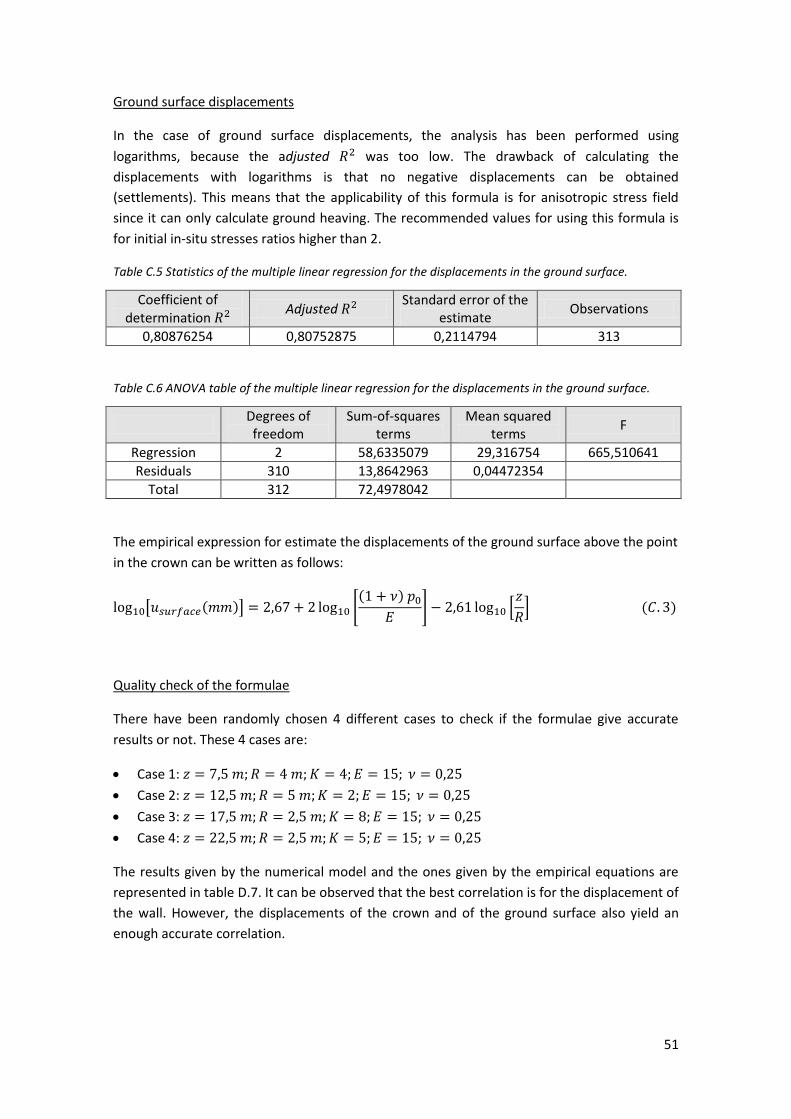
51

Ground surface displacements

In the case of ground surface displacements, the analysis has been performed using

logarithms, because the adjusted was too low. The drawback of calculating the

displacements with logarithms is that no negative displacements can be obtained

(settlements). This means that the applicability of this formula is for anisotropic stress field

since it can only calculate ground heaving. The recommended values for using this formula is

for initial in-situ stresses ratios higher than 2.

Table C.5 Statistics of the multiple linear regression for the displacements in the ground surface.

Coefficient of determination

Adjusted Standard error of the

estimate Observations

0,80876254 0,80752875 0,2114794 313

Table C.6 ANOVA table of the multiple linear regression for the displacements in the ground surface.

Degrees of freedom

Sum-of-squares terms

Mean squared terms

F

Regression 2 58,6335079 29,316754 665,510641

Residuals 310 13,8642963 0,04472354

Total 312 72,4978042

The empirical expression for estimate the displacements of the ground surface above the point

in the crown can be written as follows:

Quality check of the formulae

There have been randomly chosen 4 different cases to check if the formulae give accurate

results or not. These 4 cases are:

Case 1:

Case 2:

Case 3:

Case 4:

The results given by the numerical model and the ones given by the empirical equations are

represented in table D.7. It can be observed that the best correlation is for the displacement of

the wall. However, the displacements of the crown and of the ground surface also yield an

enough accurate correlation.

52

Table C.7 Comparison between results obtained from UDEC and results obtained from empirical

equations (in mm).

Case 1 Case 2 Case 3 Case 4

UDEC Empirical UDEC Empirical UDEC Empirical UDEC Empirical

0,36 0,39 0,33 0,34 0,97 0,97 0,99 0,82

0,15 0,14 -0,065 0,037 0,18 0,21 0,12 0,039

0,17 0,17 0,096 0,081 0,13 0,098 0,056 0,004

In figures C.1, C.2 and C.3, there are plotted the calculated displacements with the empirical

equations against the calculated displacements with UDEC. The main purpose of these graphs

is to show that the obtained empirical formulation fits rather well with the numerical results.

Figure C.1 Calculated empirical displacement against UDEC displacement for the wall.

Figure C.2 Calculated empirical displacement against UDEC displacement for the crown.

-0,5

0

0,5

1

1,5

2

2,5

3

0 0,5 1 1,5 2 2,5

Calculated displacement

100% correlation

90% confidence interval (upper)

90% confidence interval (lower)

-0,6

-0,4

-0,2

0

0,2

0,4

0,6

0,8

1

-0,5 0 0,5 1

Calculated displacement

100% correlation

80% confidence interval (upper)

80% confidence interval (lower)

53

Figure C.3 Calculated empirical displacement against UDEC displacement for the ground surface.

0

0,2

0,4

0,6

0,8

1

1,2

1,4

0 0,5 1 1,5

Calculated displacement

100% correlation

90% confidence interval (upper)

90% confidence interval (lower)

54

APPENDIX D, RESULTS FROM THE NUMERICAL ANALISIS FOR THE GRC

In this appendix, plots of the displacements vectors and magnitudes are included. Major and

minor principal stresses plots are included as well. There are plots for each one of the depths

analyzed (5; 7,5; 12,5; 17,5 and 22,5 meters) and for the initial in-situ stress values of 1, 2, 4

and 6.

In order to check that the stresses were implemented correctly with the gradient, figures 3, 16,

27, 34 and 41 represent the in-situ stress previous to excavation. It can be noticed that the

excavation-induced stresses reach a maximum (approximate) distance of three tunnel

diameters, even for cases with high initial in-situ stress ratios.

Figure D.1 Displacement vectors and magnitudes for tunnel depth of 5 meters and =1.

Figure D.2 Minor and major principal stresses for tunnel depth of 5 meters and =1.

55

Figure D.3 Minor and major principal stresses for tunnel depth of 5 meters and =1 previous to

excavation.

Figure D.4 Displacement vectors and magnitudes for tunnel depth of 5 meters and =2.

Figure D.5 Minor and major principal stresses for tunnel depth of 5 meters and =2.

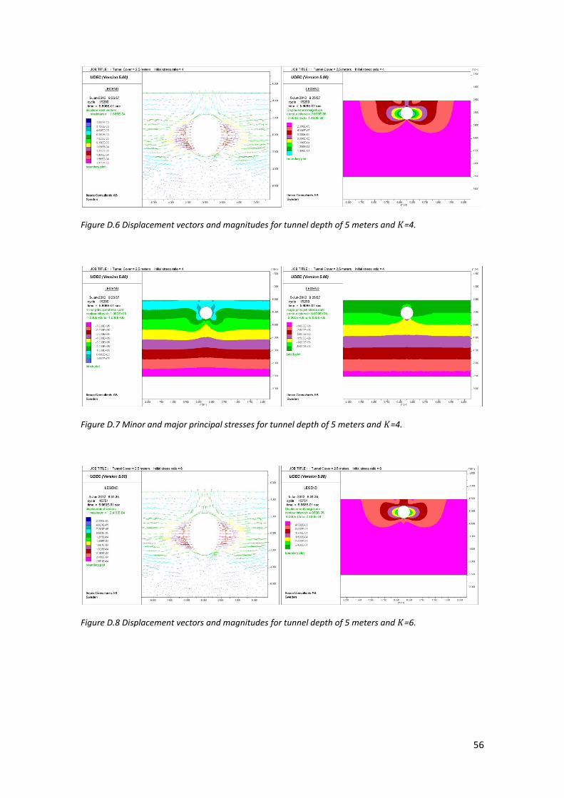
56

Figure D.6 Displacement vectors and magnitudes for tunnel depth of 5 meters and =4.

Figure D.7 Minor and major principal stresses for tunnel depth of 5 meters and =4.

Figure D.8 Displacement vectors and magnitudes for tunnel depth of 5 meters and =6.

57

Figure D.9 Minor and major principal stresses for tunnel depth of 5 meters and =6.

Figure D.10 Displacement vectors and magnitudes for tunnel depth of 7,5 meters and =1.

Figure D.11 Minor and major principal stresses for tunnel depth of 7,5 meters and =1.

58

Figure D.12 Displacement vectors and magnitudes for tunnel depth of 7,5 meters and =2.

Figure D.13 Minor and major principal stresses for tunnel depth of 7,5 meters and =2.

Figure D.14 Displacement vectors and magnitudes for tunnel depth of 7,5 meters and =4.

59

Figure D.15 Minor and major principal stresses for tunnel depth of 7,5 meters and =4.

Figure D.16 Minor and major principal stresses for tunnel depth of 7,5 meters and =4 previous to

excavation.

Figure D.17 Displacement vectors and magnitudes for tunnel depth of 7,5 meters and =6.

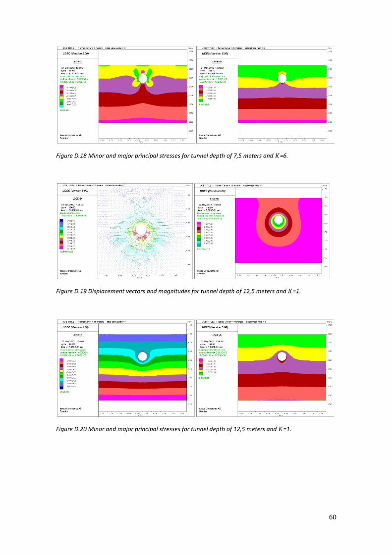
60

Figure D.18 Minor and major principal stresses for tunnel depth of 7,5 meters and =6.

Figure D.19 Displacement vectors and magnitudes for tunnel depth of 12,5 meters and =1.

Figure D.20 Minor and major principal stresses for tunnel depth of 12,5 meters and =1.

61

Figure D.21 Displacement vectors and magnitudes for tunnel depth of 12,5 meters and =2.

Figure D.22 Minor and major principal stresses for tunnel depth of 12,5 meters and =2.

Figure D.23 Displacement vectors and magnitudes for tunnel depth of 12,5 meters and =4.

62

Figure D.24 Minor and major principal stresses for tunnel depth of 12,5 meters and =4.

Figure D.25 Displacement vectors and magnitudes for tunnel depth of 12,5 meters and =6.

Figure D.26 Minor and major principal stresses for tunnel depth of 12,5 meters and =6.

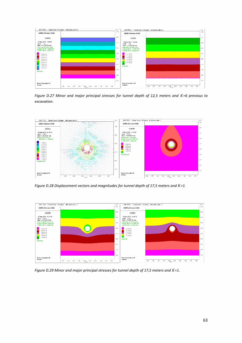
63

Figure D.27 Minor and major principal stresses for tunnel depth of 12,5 meters and =6 previous to

excavation.

Figure D.28 Displacement vectors and magnitudes for tunnel depth of 17,5 meters and =1.

Figure D.29 Minor and major principal stresses for tunnel depth of 17,5 meters and =1.

64

Figure D.30 Displacement vectors and magnitudes for tunnel depth of 17,5 meters and =2.

Figure D.31 Minor and major principal stresses for tunnel depth of 17,5 meters and =2.

Figure D.32 Displacement vectors and magnitudes for tunnel depth of 17,5 meters and =4.

65

Figure D.33 Minor and major principal stresses for tunnel depth of 17,5 meters and =4.

Figure D.34 Minor and major principal stresses for tunnel depth of 17,5 meters and =4 previous to

excavation.

Figure D.35 Displacement vectors and magnitudes for tunnel depth of 17,5 meters and =6.

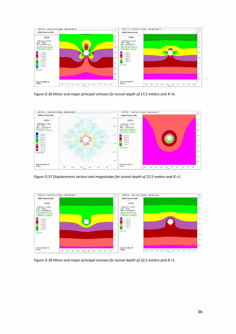
66

Figure D.36 Minor and major principal stresses for tunnel depth of 17,5 meters and =6.

Figure D.37 Displacement vectors and magnitudes for tunnel depth of 22,5 meters and =1.

Figure D.38 Minor and major principal stresses for tunnel depth of 22,5 meters and =1.

67

Figure D.39 Displacement vectors and magnitudes for tunnel depth of 22,5 meters and =2.

Figure D.40 Minor and major principal stresses for tunnel depth of 22,5 meters and =2.

Figure D.41 Minor and major principal stresses for tunnel depth of 22,5 meters and =2 previous to

excavation.

68

Figure D.42 Displacement vectors and magnitudes for tunnel depth of 22,5 meters and =4.

Figure D.43 Minor and major principal stresses for tunnel depth of 22,5 meters and =4.

Figure D.44 Displacement vectors and magnitudes for tunnel depth of 22,5 meters and =6.

69

Figure D.45 Minor and major principal stresses for tunnel depth of 22,5 meters and =6.

70

APPENDIX E, GROUND REACTION CURVES

In this appendix, there are ground reaction curves plotted for 18 different cases. These ground

reaction curves correspond to tunnel depths of 5, 7,5; 12,5; 17,5 and 22,5 meters.

The extra plots for initial in-situ stress values of 3, 5, 7, 8, 9 and 10 for depth of 5 meters are

shown from figure E.1 to E.6. To avoid repetition, only the ground reaction curves for 7,5; 12,5

and 17,5 and for initial stress ratios of , , and will be plotted in this appendix.

As in the case of 5 meters depth, in every graph, there are 4 ground reaction curves. These

ground reaction curves correspond for the analytical solution, for a point in the wall of the

tunnel, for a point in the crown of the tunnel and for a point in the floor of the tunnel.

The analytical ground reaction curves for all the cases in this appendix are also straight lines

for every case (like in the 5 meters depth tunnel).

Ground reaction curves for tunnel depth of 5 meters

Figure E.1 Ground reaction curve for =3 and tunnel depth of 5 meters.

0

0,1

0,2

0,3

0,4

0,5

0,6

0,7

0,8

0,9

1

0 0,02 0,04 0,06 0,08 0,1 0,12

Analytical

Wall

Crown

71

Figure E.2 Ground reaction curve for =5 and tunnel depth of 5 meters.

Figure E.3 Ground reaction curve for =7 and tunnel depth of 5 meters.

0

0,1

0,2

0,3

0,4

0,5

0,6

0,7

0,8

0,9

1

-0,1 -0,05 0 0,05 0,1 0,15 0,2 0,25

Analytical

Wall

Crown

Floor

0

0,1

0,2

0,3

0,4

0,5

0,6

0,7

0,8

0,9

1

-0,2 -0,1 0 0,1 0,2 0,3

Analytical

Wall

Crown

Floor

72

Figure E.4 Ground reaction curve for =8 and tunnel depth of 5 meters.

Figure E.5 Ground reaction curve for =9 and tunnel depth of 5 meters.

0

0,1

0,2

0,3

0,4

0,5

0,6

0,7

0,8

0,9

1

-0,2 -0,1 0 0,1 0,2 0,3 0,4

Analytical

Wall

Crown

Floor

0

0,1

0,2

0,3

0,4

0,5

0,6

0,7

0,8

0,9

1

-0,2 -0,1 0 0,1 0,2 0,3 0,4

Analytical

Wall

Crown

Floor

73

Figure E.6 Ground reaction curve for =10 and tunnel depth of 5 meters.

Ground reaction curves for tunnel depth of 7,5 meters

Figure E.7 Ground reaction curve for =1 and tunnel depth of 7,5 meters.

0

0,1

0,2

0,3

0,4

0,5

0,6

0,7

0,8

0,9

1

-0,2 0 0,2 0,4 0,6

Analytical

Wall

Crown

Floor

0

0,1

0,2

0,3

0,4

0,5

0,6

0,7

0,8

0,9

1

0 0,02 0,04 0,06 0,08

Analytical

Wall

Crown

Floor

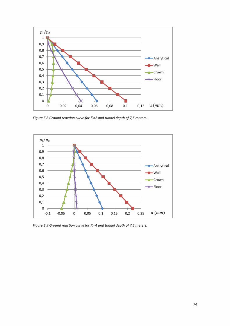
74

Figure E.8 Ground reaction curve for =2 and tunnel depth of 7,5 meters.

Figure E.9 Ground reaction curve for =4 and tunnel depth of 7,5 meters.

0

0,1

0,2

0,3

0,4

0,5

0,6

0,7

0,8

0,9

1

0 0,02 0,04 0,06 0,08 0,1 0,12

Analytical

Wall

Crown

Floor

0

0,1

0,2

0,3

0,4

0,5

0,6

0,7

0,8

0,9

1

-0,1 -0,05 0 0,05 0,1 0,15 0,2 0,25

Analytical

Wall

Crown

Floor

75

Figure E.10 Ground reaction curve for =6 and tunnel depth of 7,5 meters.

Ground reaction curves for tunnel depth of 12,5 meters

Figure E.11 Ground reaction curve for =1 and tunnel depth of 12,5 meters.

0

0,1

0,2

0,3

0,4

0,5

0,6

0,7

0,8

0,9

1

-0,2 -0,1 0 0,1 0,2 0,3 0,4

Analytical

Wall

Crown

Floor

0

0,1

0,2

0,3

0,4

0,5

0,6

0,7

0,8

0,9

1

0 0,02 0,04 0,06 0,08 0,1

Analytical

Wall

Crown

Floor

76

Figure E.12 Ground reaction curve for =2 and tunnel depth of 12,5 meters.

Figure E.13 Ground reaction curve for =4 and tunnel depth of 12,5 meters.

0

0,1

0,2

0,3

0,4

0,5

0,6

0,7

0,8

0,9

1

0 0,05 0,1 0,15 0,2

Analytical

Wall

Crown

Floor

0

0,1

0,2

0,3

0,4

0,5

0,6

0,7

0,8

0,9

1

-0,1 0 0,1 0,2 0,3 0,4

Analytical

Wall

Crown

Floor

77

Figure E.14 Ground reaction curve for =6 and tunnel depth of 12,5 meters.

Ground reaction curves for tunnel depth of 17,5 meters

Figure E.15 Ground reaction curve for =1 and tunnel depth of 17,5 meters.

0

0,1

0,2

0,3

0,4

0,5

0,6

0,7

0,8

0,9

1

-0,2 0 0,2 0,4 0,6

Analytical

Wall

Crown

Floor

0

0,1

0,2

0,3

0,4

0,5

0,6

0,7

0,8

0,9

1

0 0,02 0,04 0,06 0,08 0,1 0,12

Analytical

Wall

Crown

Floor

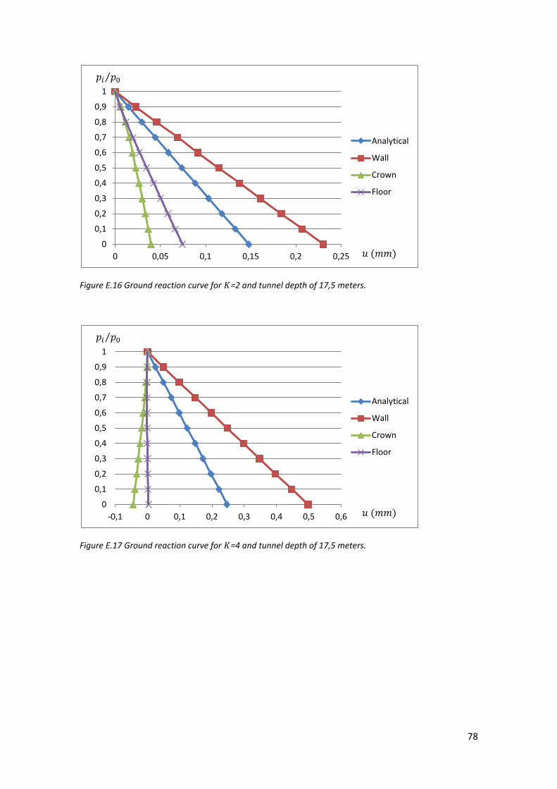
78

Figure E.16 Ground reaction curve for =2 and tunnel depth of 17,5 meters.

Figure E.17 Ground reaction curve for =4 and tunnel depth of 17,5 meters.

0

0,1

0,2

0,3

0,4

0,5

0,6

0,7

0,8

0,9

1

0 0,05 0,1 0,15 0,2 0,25

Analytical

Wall

Crown

Floor

0

0,1

0,2

0,3

0,4

0,5

0,6

0,7

0,8

0,9

1

-0,1 0 0,1 0,2 0,3 0,4 0,5 0,6

Analytical

Wall

Crown

Floor

79

Figure E.18 Ground reaction curve for =6 and tunnel depth of 17,5 meters.

0

0,1

0,2

0,3

0,4

0,5

0,6

0,7

0,8

0,9

1

-0,2 0 0,2 0,4 0,6 0,8 1

Analytical

Wall

Crown

Floor