limiting forms of the trace formula - stanford university
TRANSCRIPT

Limiting Forms of the Trace Formula
Akshay Venkatesh
A Dissertation
Presented to the Faculty
of Princeton University
in Candidacy for the Degree
of Doctor of Philosophy
Recommended for Acceptance
by the
Department of Mathematics
November 2002

c© Copyright by Akshay Venkatesh, 2002.
All Rights Reserved

Abstract
We carry out the first nontrivial cases of the limiting process proposed by Langlands
in his manuscript Beyond Endoscopy, with technical variations that enable us to treat
the limit unconditionally. This gives an elementary proof, on GL(2), of the classi-
fication of forms such that the symmetric square L-function has a pole (including,
implicitly, the construction of these forms). The result of this may be seen as one
of the simplest cases of the “pipe-dream” Langlands proposes. We also apply simi-
lar methods to derive a converse theorem, and to produce a result that generalizes
Duke’s estimate on the dimension of weight 1 forms to arbitrary number fields – but
is sharper, even over Q, than Duke’s original estimate.
iii

Acknowledgements
I was partially supported during the preparation of this thesis by a Hackett Stu-
dentship. I would like to thank the University of Western Australia for this assistance.
This thesis would not exist without the support and generosity of my advisor,
Peter Sarnak. I have learned a great deal from working with him, and it is a pleasure
to thank him now for making it such a pleasant experience; many of the ideas that
have been developed here are due to him.
I would also like to express my gratitude to Professor Robert Langlands, whose pa-
per Beyond Endoscopy was the inspiration for this work, and whose interest, support
and suggestions were most helpful.
I would like to thank all my dear friends at Princeton; I would rather not list their
names here, but merely trust that they know who I am referring to should they ever
read this.
I would finally like to thank my parents, for all their years of unconditional love
and support, without which I would not be here now.
iv

Contents
Abstract . . . . . . . . . . . . . . . . . . . . . . . . . . . . . . . . . . . . . iii
Acknowledgements . . . . . . . . . . . . . . . . . . . . . . . . . . . . . . . iv
1 Introduction 1
1.1 Limits and the Trace Formula . . . . . . . . . . . . . . . . . . . . . . 1
1.2 Langlands’ Idea . . . . . . . . . . . . . . . . . . . . . . . . . . . . . . 2
1.3 Discussion of Contents . . . . . . . . . . . . . . . . . . . . . . . . . . 3
1.3.1 Dihedral Forms . . . . . . . . . . . . . . . . . . . . . . . . . . 4
1.3.2 Rankin-Selberg Convolutions and Converse Theorems . . . . . 7
1.3.3 Higher Symmetric Powers . . . . . . . . . . . . . . . . . . . . 8
1.3.4 Related Work . . . . . . . . . . . . . . . . . . . . . . . . . . . 9
1.4 Format of Thesis . . . . . . . . . . . . . . . . . . . . . . . . . . . . . 9
2 Dihedral Forms over Q 11
2.1 Introduction . . . . . . . . . . . . . . . . . . . . . . . . . . . . . . . . 11
2.2 Preliminaries . . . . . . . . . . . . . . . . . . . . . . . . . . . . . . . 12
2.2.1 Petersson formula . . . . . . . . . . . . . . . . . . . . . . . . . 13
2.2.2 Petersson-Kuznetsov formula . . . . . . . . . . . . . . . . . . 14
2.2.3 Integral transformation formulae . . . . . . . . . . . . . . . . 15
2.3 Isolation of dihedral representations . . . . . . . . . . . . . . . . . . . 16
2.3.1 Geometric side . . . . . . . . . . . . . . . . . . . . . . . . . . 17
v

2.3.2 Translation in terms of h±, hk . . . . . . . . . . . . . . . . . . 22
2.3.3 Analysis of the local sum . . . . . . . . . . . . . . . . . . . . . 26
2.4 The standard L-function . . . . . . . . . . . . . . . . . . . . . . . . . 33
2.5 From Trace Formula to Classification . . . . . . . . . . . . . . . . . . 35
2.5.1 Expected Answer . . . . . . . . . . . . . . . . . . . . . . . . . 36
2.5.2 Right-hand side: Grossencharacters . . . . . . . . . . . . . . . 39
2.5.3 Left-Hand Side: Residues of Rankin-Selberg L-functions, new-
forms and oldforms . . . . . . . . . . . . . . . . . . . . . . . . 40
2.5.4 Contribution of the Continuous Spectrum . . . . . . . . . . . 43
2.5.5 Case of full level . . . . . . . . . . . . . . . . . . . . . . . . . 47
2.6 Putting it all together! . . . . . . . . . . . . . . . . . . . . . . . . . . 49
3 Converse Theorems 54
3.1 Introduction . . . . . . . . . . . . . . . . . . . . . . . . . . . . . . . . 54
3.2 Limiting Process . . . . . . . . . . . . . . . . . . . . . . . . . . . . . 55
3.2.1 Voronoi-type summation formulae . . . . . . . . . . . . . . . . 58
3.2.2 Analysis of S(m;X) . . . . . . . . . . . . . . . . . . . . . . . 60
3.2.3 Allowing Poles for the Twists . . . . . . . . . . . . . . . . . . 65
4 Dihedral forms over number fields 68
4.1 Introduction . . . . . . . . . . . . . . . . . . . . . . . . . . . . . . . . 68
4.2 Translation from adelic to classical . . . . . . . . . . . . . . . . . . . 71
4.2.1 Classical setting . . . . . . . . . . . . . . . . . . . . . . . . . . 71
4.2.2 Whittaker models and Fourier coefficients . . . . . . . . . . . 74
4.3 Limiting Process . . . . . . . . . . . . . . . . . . . . . . . . . . . . . 77
4.3.1 Unramified twists of quadratic extension . . . . . . . . . . . . 78
4.3.2 Kuznetsov’s formulas . . . . . . . . . . . . . . . . . . . . . . . 79
4.3.3 Constructing the sum to pick out dihedral forms . . . . . . . . 83
vi

4.3.4 Poisson Summation . . . . . . . . . . . . . . . . . . . . . . . . 85
4.4 Computation of the local sums . . . . . . . . . . . . . . . . . . . . . . 91
4.4.1 Translation of local sums to adelic integrals . . . . . . . . . . 91
4.4.2 Zeta functions . . . . . . . . . . . . . . . . . . . . . . . . . . . 93
4.4.3 Local factors of Zeta functions . . . . . . . . . . . . . . . . . . 97
4.4.4 Evaluation of measures and of zeta functions . . . . . . . . . . 101
4.5 Expected answer . . . . . . . . . . . . . . . . . . . . . . . . . . . . . 104
4.5.1 Fourier coefficients of the corresponding forms . . . . . . . . . 106
4.6 Derivation of Petersson Formula (after Cogdell, Piatetski-Shapiro) . . 110
4.6.1 Geometric Computation of Fourier Coefficients . . . . . . . . . 115
4.6.2 Spectral Computation of Fourier Coefficient . . . . . . . . . . 118
4.6.3 Normalization of Fourier Coefficients (and Comparisons) . . . 122
4.6.4 Comparison of normalizations of Fourier Coefficients . . . . . 124
4.6.5 A transformation formula . . . . . . . . . . . . . . . . . . . . 125
5 Automorphic forms of Galois type 127
5.1 Introduction . . . . . . . . . . . . . . . . . . . . . . . . . . . . . . . . 127
5.2 Higher Symmetric Powers . . . . . . . . . . . . . . . . . . . . . . . . 128
5.3 Estimate of the number of automorphic forms of Galois type . . . . . 131
5.3.1 Existence of an amplifier . . . . . . . . . . . . . . . . . . . . . 135
6 Appendix 140
6.1 Classification of Dihedral Forms . . . . . . . . . . . . . . . . . . . . . 140
6.2 Concrete Interpretation over Q . . . . . . . . . . . . . . . . . . . . . 141
6.2.1 Fourier Coefficients . . . . . . . . . . . . . . . . . . . . . . . . 144
6.2.2 Summary of Results . . . . . . . . . . . . . . . . . . . . . . . 145
6.3 Bessel Transforms and Inversion Questions . . . . . . . . . . . . . . . 146
6.3.1 Fourier transforms and Bessel Transforms . . . . . . . . . . . 146
vii

6.3.2 Inversion problem . . . . . . . . . . . . . . . . . . . . . . . . . 148
6.4 Trace formulas . . . . . . . . . . . . . . . . . . . . . . . . . . . . . . 159
6.5 L-functions . . . . . . . . . . . . . . . . . . . . . . . . . . . . . . . . 160
6.5.1 Contour Shifting . . . . . . . . . . . . . . . . . . . . . . . . . 160
6.5.2 Uniformity . . . . . . . . . . . . . . . . . . . . . . . . . . . . . 161
viii

Chapter 1
Introduction
1.1 Limits and the Trace Formula
In the most approximate terms, this Thesis is devoted to the technique of taking a
limit in a trace-type formula to isolate a spectrally “small” set of forms. In Chapters 2
and 4 the “small” set is that of dihedral forms, those corresponding to an orthogonal
2-dimensional Galois representation; in Chapter 3 we isolate a single form, and in
Chapter 5 we isolate forms of “Galois type.”
The precise theorems that can be proved with this technique vary. In Chapters
2 and 4, we give an alternate proof of the classification of dihedral forms due to
Langlands-Labesse, [12]. In Chapter 3, we show how one may derive versions of the
converse theorem from the trace formula. In Chapter 5 new estimates are obtained
for the number of automorphic forms of “Galois type.” The method of proof also
makes clear the connection of this with the amplification method now standard in the
analytic theory of automorphic forms.
The motivation for this work was the development of ideas in [13]. We now turn
to a more detailed explanation of Langlands’ idea, at least in the context we will be
using it.
1

1.2 Langlands’ Idea
We begin by discussing Langlands’ idea in relative generality; we will eventually be
somewhat more specialized in our approach.
Let AQ be the ring of adeles of Q. Let π range over all automorphic, cuspidal
representations of GL2(AQ). If ρ is a representation of the dual group GL(2,C), we
denote by m(π, ρ) the order of the pole at s = 1 of L(s, π, ρ), when defined. Let f
be a nice function on GL2(AQ); we shall denote by tr(π)(f) the trace of the operator
defined by f on the representation π.
In Beyond Endoscopy ([13]), Langlands suggests the development of a formula of
the form: ∑π
m(π, ρ)tr(π)(f) =∑
. . . (1.1)
where the right hand sum ranges over a “geometric” contribution (that is, something
resembling a sum over conjugacy classes.) This would therefore “isolate” the π for
which m(π, ρ) > 0. Such π are expected to be functorial transfers from other groups;
therefore, one might hope to be able to match the resulting formula with the trace
formulae for these groups, and thereby prove these functorial lifts. (One hopes, of
course, to do this for more general groups than GL(2).)
In concrete terms, the idea of Langlands can be expressed as follows. From the
trace formula we will be able to evaluate:
∑π
λ(n, π, ρ)tr(π)(f) = . . .
where λ(n, π, ρ) is the coefficient of n−s in the Dirichlet series L(s, π, ρ). (If ρ is the
standard representation, for example, λ(n, π, ρ) is just the nth Hecke eigenvalue.) At
least, this is true for n coprime with those primes where f ramifies – we can then
express the summand as the trace of a new function related to f . This is quite enough
2

for our purposes.
The right hand side is a geometric contribution, a sum over conjugacy classes. In
concrete terms, the most involved part (the “elliptic” term) is a sum over all quadratic
orders and involves their class numbers.
We take n = p to be prime, and sum over all p < X, weighted by log(p). For each
π, the quantity limX→∞1X
∑p<X λ(p, π, ρ) log(p) is equal to m(π, ρ). We therefore
instead evaluate:
∑π
1
Xtr(π)(f)
∑p<X
log(p)λ(p, π, ρ)
by means of the trace formula. We will then obtain a sum over primes and conjugacy
classes on the right hand side, and one can hope to evaluate the resulting limit as
X → ∞ by techniques of analytic number theory; we will then obtain a sum just
over those forms for which L(s, π, ρ) has a pole, and we will obtain an expression for
Equation 1.1, as desired.
Implicit in this is the hope of being able to identify the multiplicity of the pole of
the L-function purely from the trace formula, without recourse to integral represen-
tations; this itself is of interest. Unfortunately the technical details in inverting the
spectral sum and limit are rather formidable.
1.3 Discussion of Contents
This thesis carries through, and attempts to understand the ramifications of Lang-
lands’ idea in the first few nontrivial cases, and in a setting where the limit on the
right hand side can be evaluated.
3

1.3.1 Dihedral Forms
We continue to use the notation of the previous section. In Chapter 2, we will take ρ
to be the symmetric square representation of the dual group and use the Petersson (or
Petersson-Kuznetsov) formula instead of the trace formula and sum over all integers
rather than primes. These introduce important technical simplifications, and make
the details manageable. In some sense, it seems that for the application to dihedral
representations the Petersson formula is more natural than the trace formula. (The
method also works for ρ the standard representation, although it is not written here,
and we shall get the expected answer of 0!)
The Petersson-Kuznetsov formula, which is a central tool of the analytic theory of
GL(2), may be regarded as a “trace formula with weights”: a cuspidal form π appears
with a weight given by 1/L(1, π,Ad), where Ad is the adjoint representation (that
is, symmetric square twisted by inverse determinant.) It also includes a contribution
of the continuous spectrum. In some sense, this weight is precisely what we need for
our purposes.
For, in summing over primes, the limit limX→∞1X
∑p<X log(p)λ(p, π, ρ) is a rel-
atively harmless constant: the multiplicity m(π, ρ). In summing over integers, we
will be considering a sum of the form limX→∞1X
∑n<X λ(n, π, ρ), which essentially
evaluates the residue of L(s, π, ρ) at s = 1. This is a much less manageable weight,
because it varies in some relatively incomprehensible way as π varies. However, for
ρ = Sym2 this residue is perfectly canceled by the weights of the Petersson-Kuznetsov
formula! (Or, to be exact, for π such that L(s, π, Sym2) has a pole, the residue of
this L-function divided by L(1, π,Ad) is just 1/L(1, ωπ) where ωπ is the central char-
acter. Since we can sum over π with a prescribed central character, this is effectively
a constant.) We should stress, however, that this “miracle” is convenient but not at
all essential.
Here is a loose description of the method. We will not be dealing with the function
4

f from above any more and f will now always denote a modular form with respect
to a group Γ0(N). For such a form, let an(f) be the nth Fourier coefficient.
The Kuznetsov formula evaluates:
∑f
an(f)am(f)h(tf )
the sum ranging over an L2 basis of, say, Maass forms f of prescribed level and
Nebentypus, where 1/4+ t2f is the Laplacian eigenvalue of f . h is a test function with
various good properties, and it will show up (in a transformed fashion) on the other
side of the formula. Actually, there is a contribution from holomorphic forms and
Eisenstein series, but for ease of explanation we shall ignore these for now.
The “weight” referred to earlier enters through the difference between an(f), the
nth Fourier coefficient, and λn, the nth Hecke eigenvalue (one can regard this as the
difference between the normalization to have L2 norm one and the normalization to
have first Fourier coefficient 1; this is expressed as a value at 1 of an L-function by
Rankin-Selberg.)
We will then sum over all n < X and divide by X. (For technical reasons, we
sum with a “smooth weight function,” but this is peripheral to the concept.) We will
then obtain an evaluation of
∑f
(1
X
∑n<X
an(f)
)am(f)h(tf )
Now, as X approaches infinity, the bracketed term is merely the residue at s = 1 of
the L-function of f at zero. Of course, the standard L-function is holomorphic (for
cusp forms) and so this residue is zero. We therefore expect that the limit on the
right hand side equals 0; this is not difficult to do, and we carry it out in Chapter 2.
More interesting is the cases where one proceeds as above, but with the limit
1X
∑n<X an2(f). In that case, we are (more or less) evaluating the residue at s = 1 of
5

the symmetric square L-function, and in that case this will be nonzero precisely for
the forms originally constructed by Maass: those associated to Grossencharacters of
quadratic fields! One expects, in carrying out the limiting process on the right hand
side, both to be able to construct these forms and to show that they exhaust all forms
f for which L(s, Sym2f) has a pole at s = 1.
To be precise, carrying this through gives amounts (more or less, ignoring com-
plications of continuous spectrum) to evaluating:
∑f :m(f,Sym2)=1
λm(f)h(tf )
where λm(f) is the mth Hecke eigenvalue of f . To give the flavor of the answer, a
special case (with m = 1, and other simplifications) of what we show is the following
Theorem. (We introduce somewhat ad hoc notation to avoid having to define all the
notation of Chapter 2.)
Theorem 1. (Special case of Chapters 2 and 4) Let o be an order of the real quadratic
field Q(√D), and let N be the discriminant of o. Fixing an embedding of Q(
√D) into
R, let ε0 be a positive fundamental unit for o×; set δ = 1 or 2 according to whether,
respectively, Norm(ε0) = 1 or Norm(ε0) = −1, and let h(o) be the class number of o.
Let h be any test function on R. Let f vary over cuspidal Maass newforms of level
dividing N and Nebentypus χD, the quadratic character associated with Q(√D); for
such f , let tf be defined so that f has eigenvalue 1/4 + t2f . Then
∑f :m(f,Sym2)=1
tf 6=0
h(tf ) =h(o)
δ
∑k∈Zk 6=0
h(kπ
δ log(ε0)) (1.2)
Although this is not precisely in the form of Equation 1.1, it is nevertheless pre-
cisely a formula of the type desired: if it is known for all m and a sufficiently large
class of test functions h, it amounts to a construction and classification of all forms
6

with m(f, Sym2) = 1.
These results are known, of course: the construction of the forms is due to Hecke
[9] (in the holomorphic case) and Maass [14] (in the Maass-form case), and the clas-
sification follows from works of Gelbart-Jacquet [7] and Labesse-Langlands [12].
However, the proof contained here is quite different. It is also very concrete: one
sees the fundamental units of quadratic fields arise in a remarkable hands-on fashion!
On the other hand, this obscures some of the conceptual generality, and it may be
difficult to carry this out for more general groups.
Chapter 4 is primarily technical in nature and discusses the generalization of this
to number fields. We focus, in particular, on the case of a totally real field, but
the discussion there is primarily intended to sketch that the same procedure can be
done over any fields; in particular, the units do not intervene dangerously, as they
sometimes do in analytic investigations of this nature.
Remark 1. The natural definition of a “dihedral” automorphic form is one that is
associated to a representation of the Weil group with dihedral image. This is more
general than requiring that the symmetric square have a pole, as a dihedral subgroup
of GL(2,C) need not be conjugate to a subgroup of O(2,C). The classification of
these, more general, dihedral representations could be effected by this technique; one
would incorporate a twist by a Dirichlet character.
1.3.2 Rankin-Selberg Convolutions and Converse Theorems
A second application, also suggested by Langlands is the following: rather than aver-
aging the residue of L(s, Sym2f) over the spectrum, average the residue of L(s, f×σ),
where σ is a Galois representation. Of course, it is not entirely clear what this means,
since this L-function is not even well-defined! (At best, one can define it as a mero-
morphic function, using base change, for σ solvable.) Nevertheless, one might hope
to obtain nontrivial information in the direction of modularity in this fashion.
7

It turns out that what one obtains from this is a version of the converse theorem
for σ! To be exact, this gives an “analytic” version of the converse theorem, which
implies the converse theorem in the form of “functional equations and analyticity of
all twists implies modularity.” It is of some interest as it shows how the trace formula
(or the Petersson-Kuznetsov formula) leads naturally to a converse theorem. It would
be of interest to see if this can be duplicated for other groups.
1.3.3 Higher Symmetric Powers
Finally, in Chapter 5 we discuss applying the same procedure to a higher symmetric
power than the second. This, of course, also has a relation to Galois representations:
for example, one expects that the forms f with m(f, Sym12) = 1 are precisely those
f parameterized by an icosahedral Galois representation!
After briefly summarizing the reasons why the naive generalizations do not work
– this was pointed out by Sarnak [17] – we then show how the same techniques can
be used to improve on Duke’s bound on the dimension of the space of holomorphic
weight 1 forms.
We work over a number field in Chapter 5. A special case of what we prove is the
following result over Q:
Theorem 2. (Special case of Chapter 5) Let χ be a Dirichlet character of modulus
q. Let S1(q, χ) be the C-vector space of weight 1 holomorphic forms of level q and
Nebentypus χ. Then, for all ε > 0, one has the bound
dim S1(q, χ) ε q6/7+ε
This sharpens a result of Duke, who proved the corresponding bound with 67
replaced by 1112
.
8

1.3.4 Related Work
Duke kindly brought to my attention the work of Mizumoto [16]. This relates to what
is being done in Chapters 2 and 4. Indeed, Mizumoto is analytically continuing the
symmetric square L-functions in the special case of holomorphic forms of full level
over fields of class number 1. His method, when unwound, is similar to ours: the
Poincare series he uses is closely related to the Petersson formula that we use (or
vice versa!), and he carries out a limit, encountering Kloosterman sums in a similar
context. In Mizumoto’s setting, one does not encounter the issue of a pole at all – the
central point of this work – and the emphasis is quite different (in the holomorphic
setting one does not encounter many of the difficulties associated with the infinite
dimensional Maass-form type spaces where we work) but the basic ideas are similar.
1.4 Format of Thesis
The format of this thesis is as follows: Chapter 2 is devoted to carrying through
the process outlined above, over Q, and in Chapter 3 the relation of these ideas to
converse theorems is outlined – not in maximal generality, but in a special case that
indicates, essentially, how one obtains the conditions on L-functions that arise in the
converse theorem out of the trace formula. In Chapter 4, we sketch the modifications
necessary to work over a number field. This involves a derivation of the Petersson-
Kuznetsov formula; forms of this do exist, but it is most convenient for our purpose
to derive a particular form following the representation-theoretic ideas of Cogdell-
Piatetski-Shapiro. In Chapter 5, we show the applicability of an approximate version
of this technique, when one relaxes the requirement for exact results and merely
aims for estimates. The consequence will be a generalization of a result of “Duke
type” to number fields; it is, even over Q, sharper than Duke’s original bound. (This
generalization – in the context of the “amplification method” – was independently
9
and essentially simultaneously observed by P. Michel; see [15]).
The Appendix gathers together several points not treated in the text. It discusses,
in terms of Langlands’ philosophy and the translation to more concrete data, the
expected parameterization of dihedral forms. It also contains a density result for
Bessel transforms, a discussion of trace-type formulas and some results on partial
sums of coefficients of L-series.
Chapters 2, 3 and 4 are, more or less, independent; although there are various
cross-references, they are not essential for reading purposes. Chapter 5 depends to
a slight extent on Chapter 4 for background, but is also essentially self-contained.
Chapter 4 is also the most involved, technically and notationally, and it is probably
better to read Chapter 2 to get a feel for the underlying idea.
There is an index of notation that precedes the bibliography, which may be of
assistance in navigating this thesis.
Finally, a word on notation that will be used throughout this thesis: an ε which
is otherwise undefined means “the formula is valid for any positive value of ε.” For
example, f(x) xε means that the function f grows slower than any positive power
of x. The implicit constant of the , however, depends on ε.
10
Chapter 2
Dihedral Forms over Q
2.1 Introduction
This Chapter carries through, in the context of forms over Q, the procedure outlined
in the introduction to isolate those “dihedral” forms f such that L(s, f, Sym2) has a
pole at s = 1.
The main result of the Chapter is the “trace formula” over dihedral forms: a
linear functional that averages the residue of the symmetric square L-function over the
spectrum. It is obtained in Proposition 3 and rewritten more conveniently in Equation
2.16 and Equation 2.18. This leads formally to the construction and classification of
these dihedral forms: see Theorem 4 in Section 2.6. We only sketch the argument
leading from the trace formulae to the classification, as it is relatively standard.
The main purpose of the Chapter is the proof of the Theorem using the limiting
technique, and we have not attempted to make our proof as “minimalistic” as possible.
In particular, we appeal to knowledge of integral representations of Rankin-Selberg
L-functions and the symmetric square L-function; this does not compromise the result
in any way, and streamlines the exposition.
As mentioned in the Introduction to this Thesis, this theorem is known, but the
11

proof here is of an entirely different nature to previous ones.
In Section 2, the required trace formulae of Petersson and Kuznetsov are stated,
along with integration transformation formulae (proved in Appendix.)
In Section 3, we carry out the limiting process, and obtain the resulting “trace
formula over dihedral forms”: see Equations 2.16 and Equation 2.18.
In Section 4, we briefly discuss the case (in the language of the Introduction to
this thesis) of ρ = St, the standard representation; we show how the same process as
in Sections 2 and 3 shows that m(f, St) = 0 for all forms (and, indeed, a still stronger
result.)
In the final two sections, we sketch the passage from a trace formula to the clas-
sification Theorem 4. There is essentially only one non-formal part to this, which
is a density assertion for the spectral test functions (which can be happily assumed
without loss of continuity, but is derived in Section 6.3.2 of the Appendix.) However,
there are other interesting issues which arise, most notably the contribution of the
continuous spectrum to the answer.
(The Appendix contains various relatively well-known results that are relevant to
this Chapter: the translation from classical to adelic language and various results on
Bessel functions.)
2.2 Preliminaries
Let χ be a Dirichlet character to the modulus N . If N divides c, we define the
Kloosterman sum Sχ(m,n, c) via:
∑(Z/cZ)×
χ(x)e((mx+ nx−1)/c)
in which χ is regarded as a character of (Z/cZ)×, because N divides c. Here, as
always, we define e(α) = e2πiα.
12

We refer to Iwaniec’s book [10], for a derivation of the Petersson and Kuznetsov
formulae that we shall use. The notation we use is also based on Iwaniec’s book.
Throughout this thesis, we will be using “smooth summation.” That is, we will
fix a C∞ function g(x) compactly supported in (0,∞) and of integral 1, and, given
a sequence of numbers cn, will usually use∑
n g(n/X)cn rather than∑
n<X cn. This,
for technical reasons, is very convenient. When it is not necessary to make the
smooth function explicit, we shall use the notation∑
n∼X cn, meaning the sum with
an appropriate smooth weight function of integral 1; it should be thought of as a
smoothed version of∑
n<X cn.
2.2.1 Petersson formula
We begin by stating the “classical” Petersson formula. Let Sk(Γ0(N), χ) be the space
of holomorphic cusp forms of weight k for the group Γ0(N), with Nebentypus χ. We
must have (−1)k = χ(−1); else, the space is trivial. For each form f ∈ Sk(Γ0(N), χ),
let cn(f) be the nth Fourier coefficient, and define:
an(f) =
√(k − 2)!
(4π)k−1cn(f)/n(k−1)/2
Then:
∑f
an(f)am(f) = δmn + 2πik∑
c≡0 modNc>0
1
cSχ(m,n; c)Jk−1(
4π√mn
c) (2.1)
The sum is over an orthonormal basis for Sk(Γ0(N), χ), with respect to the Pe-
tersson inner product.
13

2.2.2 Petersson-Kuznetsov formula
This formula was generalized by Kuznetsov, to give a formula that includes Maass as
well as holomorphic forms – in other words, the whole spectrum.
Let χ be a Dirichlet character to the modulus N .
∑f
hf (ϕ)an(f)am(f) +∑
c
1
4π
∫ ∞
−∞h±(t)ηc(n, 1/2 + it)ηc(m, 1/2 + it)dt
=∑
c≡0(modN)c>0
1
cϕ(
4π√|nm|c
)Sχ(n,m; c) (2.2)
ϕ is a compactly supported function on (0,∞). The left hand summation ranges over
an orthonormal basis for modular forms f with respect to (Γ0(N), χ), holomorphic
and Maass. The sum over c is over cusps. The definitions of h± and hf (ϕ) are given
below. The an(f) and ηc are the Fourier coefficients of cusp forms and Eisenstein
series respectively, normalized so to be of size around 1.
To be precise, given a Maass cusp form f with L2 norm 1 and eigenvalue 1/4+s2,
one may write its Fourier expansion:
f(z) =∑n6=0
ρ(n)Ws(nz)
where Ws(x+ iy) = 2√yKs−1/2(2π|y|)e(x). One then defines:
an(f) =
(4π|n|
cosh(πs)
)1/2
ρ(n)
The normalization for the Fourier coefficients of holomorphic forms is as in the Pe-
tersson formula. The normalization for the Eisenstein series is similar to that in the
case of Maass cusp forms; we refer to Iwaniec for details in that case.
hf = hf (ϕ) is a weight function, and the map between ϕ and hf (ϕ) is given by an
14

appropriate integral transform that is explicated below; in fact, hf (ϕ) depends only
on the Laplacian eigenvalue (or “infinity type”) of f .
(It is convenient to think of the Petersson formula, Equation 2.1, as being a
form of Equation 2.2, where hf = 1 exactly for those forms f of weight k, and
ϕ(x) = 2πikJk−1(x). This is not precisely accurate, as the Petersson formula involves
an additional “diagonal term” δmn, which is closely related to the fact that this choice
of ϕ is not compactly supported. However, this δmn will make no difference to our
analysis: it will drop out in the limit.)
Let Jν , Kν denote the usual J- or K- Bessel function. The functions hf (ϕ) and
h±(t) are given as follows:
1. When f is a holomorphic form of even weight k, it equals hf (ϕ) = hk =
ik∫∞
0ϕ(x)Jk−1(x)x
−1dx.
2. If f is a Maass form or Eisenstein series of eigenvalue 1/4+t2f it varies, according
to the sign of the product nm.
(a) If nm > 0, then hf (ϕ) = h+(tf ), where h+(tf ) =∫∞
0B2itf (x)ϕ(x)x−1dx,
and Bν(x) = (2 sin(πν/2))−1(J−ν(x)− Jν(x)).
(b) If nm < 0, then hf (ϕ) = h−(tf ) = 4π
cosh(πtf )∫∞
0K2itf (x)ϕ(x)x−1dx.
The Kloosterman sum Sχ(m,n; c) is as defined before.
2.2.3 Integral transformation formulae
Since we will be applying Poisson summation, we will have need of the following inte-
gral transforms, which can be derived easily from the formulae for Fourier transforms
of Bessel functions. These are derived in the Appendix.
First, some remarks on Fourier transform and its normalization. Let f(x) be
a function on R; its Fourier transform is f(k) =∫∞−∞ f(x)eikxdx. Then f(x) =
15

12π
∫∞−∞ f(k)e−ikxdk. With this normalization, the Fourier transform of the constant
function 1 is the distribution 2πδ, where δ is the measure of mass 1 supported at 0,
and the Fourier transform of f(x)g(x) is (1/2π)f ? g, where ? is convolution.
Let ϕ and h± be related as in the previous Subsection. Let ∆(λ) be the Fourier
transform of ϕ(x)/x and h± the Fourier transform of h±. We have the formulae:
h−(λ) = h−(−λ) =1
2(∆(sinh(λ/2)) + ∆(− sinh(λ/2))) (2.3)
h+(λ) = h+(−λ) =1
2(∆(cosh(λ/2)) + ∆(− cosh(λ/2))) (2.4)
If k is odd, we also have the following, with ϕ(x) = 2πikJk−1(x):
1
2(∆(λ)+∆(−λ)) =
∫ ∞
0
cos(λx)ϕ(x)
xdx =
2πik
k−1cos((k − 1) arcsin(λ)), |λ| ≤ 1;
(−1)(k−1)/2) 2πik
k−1e−(k−1) cosh−1(λ), |λ| ≥ 1
(2.5)
2.3 Isolation of dihedral representations
We will now prove the main result. The limiting process on the geometric side is
carried out in the first subsection: see Proposition 3.
We will work in the following context. Let D be a fundamental discriminant.
By this we mean that |D| should be the discriminant of Q(√D); it is possible D
is negative. Let χ = χD be the quadratic character(D·
), that is, the quadratic
character associated to Q(√D). It is a Dirichlet character to the modulus |D|. Let f
be an integer and let N = |D|f 2. One expects to find “dihedral” forms, those whose
symmetric square has a pole, on the group Γ0(N) with Nebentypus χ, and indeed we
expect all dihedral forms will occur in this way as we vary N .
In the limiting process, the treatments for D > 0 and D < 0 vary slightly from
16

each other. The exposition in the text will focus on the case D > 0 and will indicate
the (very minor) changes needed for the case D < 0.
It is convenient to make the following:
Definition 1. Define a constant c(N) as follows:
c(N) =
(√
N∏
p|N(1 + 1/p))−1
, D > 0
i(√
N∏
p|N(1 + 1/p))−1
, D < 0
It is not really a function only of N – it would probably be better denoted c(N,χ),
but it will be clear from context what is going on, since when we use it we will be
dealing with D > 0 and D < 0 separately.
Format of this section: In Subsection 2.3.1, the limiting process is carried out.
In doing so, certain information about some local sums is required – we borrow the
results from Subsection 2.3.3, where they are proved. The result for the limit L is
in Equation 2.13. In Subsection 2.3.2, we translate the results from the “geometric
side” function ϕ to being in terms of the “spectral side” functions h±.
2.3.1 Geometric side
We will work in the space of modular forms for (Γ0(N), χ), either applying the
Petersson-Kuznetsov formula in the case where D > 0, or just the Petersson for-
mula if D < 0; with this understood, the analysis proceeds identically for both cases,
with ϕ an appropriate Bessel function in the latter case. If D < 0 we will choose an
odd integer k, and will apply the Petersson formula to holomorphic forms of weight
k.
Let g be a compactly supported, positive, C∞ function on (0,∞). We will assume
∫ ∞
0
g(x)dx = 1
17

Its precise behavior is unimportant; it is only used to truncate the sums smoothly
and it will vanish from the analysis eventually.
We will be analyzing the asymptotic behavior of the sum
limX→∞
(1
X
∑f
hf (ϕ)∞∑n=1
g(n/X)an2(f)am(f)
)+ (2.6)(
1
X
∞∑n=1
g(n/X)∑
c
1
4π
∫ ∞
−∞h±(t)ηc(n
2, 1/2 + it)ηc(m, 1/2 + it)
)
This sum is meant to average over the spectrum (weighted by the function function
function function hf ) the residue of the symmetric square L-function.
The sign of h± is determined according to whether m > 0 or m < 0. The
interpretation is slightly different if D < 0: in that case, there is no integral and the
sum is over an orthonormal basis for Sk(Γ0(N), χ). In other words, hf (ϕ) should be
regarded as being supported (in the f aspect) on holomorphic forms of weight k.
We will often simply refer to the integral term as the “Continuous Spectrum
Contribution.” As will be seen in Subsection 2.5.4, it may be explicitly evaluated.
We will be assuming that (m,N) = 1, for convenience. We will denote the limit
of Equation 2.6 (it exists, as we will prove!) by L. It depends on m,D,N and ϕ.
The Petersson-Kuznetsov formula shows that Equation 2.6 equals:
∑f hf (ϕ)
∑n g(n/X)an2(f)am(f) + (Continuous Spectrum Contribution)
X
=1
X
∑N |c
1
c
∑n
g(n/X)ϕ(4π√m
cn)Sχ(n
2,m, c) (2.7)
If D < 0 we apply the Petersson formula in the form Equation 2.1. In that
case, the formula is as above, but there does not exist a continuous spectrum con-
tribution, the left-hand side sum is only over holomorphic forms of weight k, and
ϕ(x) = 2πikJk−1(x). (As remarked previously, the contribution of the term δnm from
Equation 2.1 vanishes in taking the limit as X →∞.)
18

We will need the following assumption on ϕ:
Hypothesis 1. There is a positive integer K so that |ϕ(x)| min(x−1/2, xK), and, for
all k ≤ K, the kth derivative |ϕ(k)(x)| k 1.
We will need K to be sufficiently large; just how large will come out from the
proof. In particular, in the case of D < 0 and holomorphic forms of weight k, this
proof will only apply for k sufficiently large; otherwise the Bessel function Jk−1(x)
will not satisfy Hypothesis 1.
We expand out the Kloosterman sum and split the n-sum into arithmetic progres-
sions mod c, so we write n = k + λc with k defined mod c and λ ∈ Z. Equation 2.6
then becomes:
1
X
∑N |c
1
c
∑k∈Z/cZ
x∈(Z/cZ)×
χ(x)e(mx−1 + k2x
c)
∑n∈Z,n≡k (c)
g(n
X)ϕ(4π
√mn
c) (2.8)
We apply Poisson summation to the n sum; let ν be the Fourier-transform pa-
rameter. This gives:
1
X
∑N |c
∑ν∈Z
1
c2
∑x∈(Z/cZ)×
k∈(Z/cZ)
χ(x)e(k2x+mx−1 − νk
c)
(∫ ∞
−∞e(νx
c)g(
x
X)ϕ(4π
√mx
c)dx
)
(2.9)
It is now convenient to define the local sum:
A(ν; c,m) =∑
k∈(Z/cZ),x∈(Z/cZ)×
e(k2x+mx−1 − νk
c)χ(x) (2.10)
At this point, some discussion of convergence in Equation 2.9 is necessary:
Proposition 1. Suppose that K ≥ 4. The double sum in Equation 2.9 converges
absolutely. If one truncates the ν sum to the range |ν| ≤ Xδ, for any fixed δ > 2K−3
,
this does not affect the limit as X →∞.
19

Proof. Repeated integration by parts shows that, if ν 6= 0,
∫ ∞
−∞e(νx
c)g(x/X)ϕ(4π
√mx
c)dxk X|
ν
c|−k min(X, c)−k = X|ν|−kmax(1, (
c
X)k)
for each k ≤ K. On the other hand, the assumed decay ϕ(x) min(1, xK) demon-
strates that, using a crude absolute-value bound,∫xe(νx
c)g(x/X)ϕ(4π
√mx
c)dx
X min(1, (Xc)K). We put these estimates together, using the first bound for small c
and the second bound for large c. Let T ≥ 1 be a parameter to be determined. Using
the trivial bound on the local sum |A(ν; c,m)| ≤ c2, we see that the total contribution
of a given value of ν to Equation 2.9 is bounded by:
1
X
∑c
∣∣∣∣(∫x
e(νx)g(x
X)ϕ(4π
√mx
c)dx
)∣∣∣∣ |ν|−K∑c<XT
max(1, (c
X)K) +
∑c>XT
(X
c)K
K X(|ν|−KTK+1 + T−K+1) (2.11)
The optimal value is T =√ν, which gives a bound of O(X|ν|1/2−K/2). On the other
hand, for ν = 0 the bound of Xmin(1, (Xc)k) shows the absolute convergence of the c
sum.
Both assertions of the Proposition now follow easily.
Now we return to our analysis, knowing that the range of the ν sum can be
taken “not too large” compared to X. Substituting the definition of A(ν; c,m), and
replacing x by cx in the integral, Equation 2.9 becomes:
1
X
∑ν∈Z
∫ ∞
−∞e2πiνx
∑N |c
A(ν; c,m)
cg(cx
X)
ϕ(4π√mx)dx (2.12)
The idea of the rest of the evaluation may be described as follows: for most values
of ν, the inner sum, which is just a smoothed version of the sum∑
cA(ν; c,m)/c,
will exhibit cancellation. These values of ν will contribute only o(X) to our sum;
20

their contribution vanishes as X → ∞. For certain values of ν, however, the inner
sum will not exhibit cancellation, and these will dominate in the limit as X → ∞.
These “special” values of ν will be identified in Section 2.3.3, and will correspond to
solutions of Pell equations, and hence to units of quadratic fields. In particular, we
can deduce the following:
Proposition 2. Let x be an integer. We define δ(x) as follows:
δ(x) = c(N), if x = Ny2 for y 6= 0, y ∈ Z
δ(x) = c(N)/2, if x = 0
δ(x) = 0, else
Let α > 0. Then there exists an absolute A > 0 so that:
∑N |c
A(ν; c,m)
cg(cα) =
6
π2
δ(ν2 − 4m)
α+Oε((1 + |ν|)Aα−1/2−ε)
Proof. This follows by expressing the right-hand side as an integral of the Mellin
transform of g against the zeta-function Z(s) associated to A(ν; c,m), shifting con-
tours, and using the properties of Z(s) given in Theorem 3 (see Subsection 2.3.3).
(See also the section 6.5 of the Appendix for some more details on this technique.)
Denote by ∆ the Fourier transform of ϕ(x)/x. Applying Proposition 1 and Propo-
sition 2, we find that Equation 2.12 becomes, for any δ > 2K−3
,
6
π2
∑ν∈Z
δ(ν2 − 4m)∆(ν
2√m
) +O(∑ν<Xδ
(1 + |ν|)AX−1/2+ε)
So long as δ is sufficiently small (i.e. K is sufficiently large) the error term is o(X).
Substituting the definition of the function δ(x), this becomes:
21

Proposition 3. The limit L of Equation 2.6 exists and equals:
L = c(N)6
π2
∑ν∈S′
′∆(
ν
2√m
) (2.13)
Here c(N) is given in Definition 1, S′ is the set of integers ν such that ν2−4m = Ny2
for some integral y, ∆ is the Fourier transform of ϕ(x)/x, and by∑′ one mean the
sum taken over ν ∈ S′ but with the contribution of any ν2 = 4m halved.
Remark 2. One can check that the constant A may be taken to be 1/2 + ε.
Checking the points at which we invoked Hypothesis 1, we see that it would have
sufficed for our argument to take K = 10. In particular, this applies to the Bessel
function ϕ(x) = Jk−1(x) so long as k ≥ 11; therefore, the arguments here apply to
holomorphic forms of weight greater than or equal to 11.
Since, at the end of this Chapter, we indicate how to modify the procedure to
apply to all holomorphic forms – including those of weight 1 – we do not aim for
optimality here.
2.3.2 Translation in terms of h±, hk
In the previous section, the limit was computed in terms of ϕ; here we translate
Equation 2.13 to a formula in terms of the spectral test functions h±, hk, incorporating
also an explicit identification of the set S′ in terms of fundamental units.
It is important to note that the resulting formulae, a priori, hold only for those
h+ that are associated to ϕ satisfying Hypothesis 1; however, a density argument,
discussed in the final section of this Chapter, extends it to all functions.
This difficulty does not occur in the holomorphic case. In view of the necessity
for ϕ to satisfy the decay condition near 0 prescribed by Hypothesis 1, the Petersson-
formula argument only applies to weights k 1. However, as commented on in the
Remark in the final section of this Chapter, this restriction can be removed by a more
22

elaborate argument involving the Petersson-Kuznetsov formula and not merely the
Petersson formula. The necessity of such an argument can perhaps be seen by noting
that in the case of weight 1 holomorphic forms, no Petersson formula exists at all
(they are not even spectrally isolated).
Maass case (D > 0)
In this section we consider the caseD > 0. We expect to find lifts of Grossencharacters
of the quadratic field Q(√D). Assume first that m > 0, so we are dealing with the
transform ϕ → h+ and we wish to express the results in terms of h+; this will be
done by applying the transformation formula Equation 2.4.
The set S′ used in Proposition 3 is ν : ν2 −Df 2y2 = 4m for some y. In other
words, m is the norm of the element 12(ν−
√Ny) in the quadratic order of discriminant
N contained in Q(√D). Let oD,f be this order in Q(
√D) of discriminantN ; explicitly,
it is Z + foD, where oD is the ring of integers of Q(√D). We also fix an embedding
of Q(√D) into R with respect to which we may speak of an element of Q(
√D) being
“positive.” Let o(1)D,f be the set of units in oD,f that have norm 1.
We then have a map
x ∈ oD,f ,Norm(x) = m → S′ (2.14)
given by x 7→ tr(x). One verifies that this map is surjective, and the fibre above ν
has size 2 unless ν2 = 4m; in that case, it has size 1. This explicit identification of
S′ permits a further simplification of Proposition 3.
Let Xm be a set of representatives, modulo o(1)D,f , for elements x ∈ oD,f such that
Norm(x) = m. (We will choose each representative x to be positive; this can be done
since we may replace x by −x.) In future sections we will often say modulo units
when we mean modulo units of positive norm, i.e. modulo o(1)D,f .
23

Let ε0 be a fundamental unit of o×D,f . Set δ = 2 if Norm(ε0) = −1 and set δ = 1
if Norm(ε0) = 1. A generator for o(1)D,f/±1 is then εδ0. Again, we may assume that
εδ0 is positive, changing the sign of ε0 if not.
Now, for ν ∈ S′, cosh−1(ν/2√m) = log(ν±
√ν2−4m
2√m
). Using some elementary ma-
nipulation (we group together the terms involving ν and −ν and then apply Equation
2.4), we see that:
∑ν∈S′
′∆(
ν
2√m
) =∑x∈Xm
∑k∈Z
h+(2(log(x√m
) + k log(εδ0))) (2.15)
Here h+ is the Fourier transform of h+. Notice at this point the importance of∑′,
which halves the contribution of ν = ±2√m, as opposed to usual sum – it “accounts”
for the varying fibre sizes in the map of Equation 2.14. Applying Poisson summation
to each inner sum in Equation 2.15, we obtain
1
2δ log(ε0)
∑k∈Z
2πh+(πk
log(εδ0))∑x∈Xm
e
(klog(x/
√m)
log(εδ0)
)
We have thus proven:
Proposition 4. Suppose D > 0 and m > 0. The limit L of Equation 2.6 exists and
equals:
L = c(N)6
πδ log(ε0)
∑k∈Z
h+(πk
δ log(ε0))
(∑x∈Xm
e
(klog(x/
√m)
log(εδ0)
))(2.16)
Here c(N) is as in Definition 1, ε0 is a fundamental unit for the order oD,f of dis-
criminant N , Xm is a set of representatives for elements of oD,f of norm m, modulo
units in o(1)D,f , and δ is 1 or 2 according to whether Norm(ε0) is 1 or −1.
Now suppose m < 0. The set S′ now consists of ν so that ν2 −Ny2 = −4|m| for
some y. For such a ν, sinh−1(ν/2√|m|) = log(ν±
√ν2−4m
2√|m|
), the choice of sign depending
24

on the sign of ν. Now let Xm be a set of (again positive) representatives of elements
oD,f with norm m modulo units. Using Equation 2.3 rather than Equation 2.4, one
sees that the limit L exists and equals:
L = c(N)6
πδ log(ε0)
∑k∈Z
h−(πk
δ log(ε0))
(∑x∈Xm
e
(klog(x/
√|m|)
log(εδ0)
))(2.17)
Holomorphic forms, weight k
Now we consider the caseD < 0. In other words, our spectral sum is over holomorphic
forms, and we are hoping to find holomorphic forms associated to Grossencharacters
of Q(√D). Again, let oD,f be the order contained in Q(
√D) of discriminant N .
Again, the set S′ consists of ν such that ν2−Df 2y2 = 4m for some y; this is now
a finite set. Let Xm be the set of elements x ∈ oD,f such that Norm(x) = m. We do
not quotient by the action of the unit group (yet!)
Xm maps to the set S′ via Trace : ν+fy√D
27→ ν; the fibres have size 2 except for
ν2 = 4m, where they have size 1.
For ν ∈ S′, we must have | ν2√m| ≤ 1, and we apply the integral transformation
formulae 2.5 to Equation 2.13. With a little manipulation, one obtains:
∑ν∈S′
′∆(
ν
2√m
) = (−1)(k−1)/2 2πik
k − 1
1
2
∑x∈Xm
(x√m
)k−1
Since x ∈ Xm =⇒ −x ∈ Xm, the inner sum vanishes unless k is odd. From
Equation 2.13, we deduce that the limit L equals:
L = −ic(N)6
π(k − 1)
∑x∈Xm
(x√m
)k−1
Let Λ(f) be the group of units in oD,f ; let wf be its cardinality. It is the cyclic
group of wf -th roots of unity. The set Xm is closed under multiplication by Λ(f)
and the sum above vanishes unless k is congruent to 1 modulo wf . Let Xm be the
25

quotient of Xm by units: so, as before, Xm is a set of representatives for elements of
norm m modulo units.
Proposition 5. Suppose D < 0 and we are computing in the space of weight k forms,
k ≥ 11. The limit L of Equation 2.6 exists and equals 0 unless k ≡ 1 mod wf ; in that
case,
L = −ic(N)6wf
π(k − 1)
∑x∈Xm
(x√m
)k−1
(2.18)
Here c(N) is as in Definition 1, Xm is a set of representatives for elements in the
order oD,f of norm m modulo o×D,f , and wf is the number of roots of unity in oD,f .
Note that here D < 0 and so c(N) is i times a positive constant. Consequently L
is real (as we expect).
2.3.3 Analysis of the local sum
We now turn to the analysis of the local sum:
A(ν; c,m) =∑
k∈Z/cZx∈(Z/cZ)×
e(−kν + k2x+mx−1
c)χ(x) =
∑k∈Z/cZ
x∈(Z/cZ)×
e(x−1k2 − kν +m
c)χ(x)
The latter expression follows from the former via replacing k by kx−1. Recall that
χ is the quadratic character χD =(D·
), although the following analysis will work
equally well in general. Our treatment will be somewhat sketchy at the prime 2; the
methods of Chapter 4 will treat that case in a more general setting.
We will prove the following:
Theorem 3. Define δ(x), for x ∈ Z, as in Proposition 2. Define, for ν,m ∈ Z, the
Dirichlet series:
Z(s) =∑N |c
A(ν; c,m)
cc−s
26

Then Z(s) has meromorphic continuation to the complex plane. It is holomorphic
in <(s) > 1/2, except for a possible simple pole at s = 1. This pole has residue
6π2 δ(ν
2 − 4m); in particular, it exists if and only if ν2 − 4m = Ny2, for some integral
y.
The function Z has at most polynomial growth in vertical strips. This is uniform
in ν, in the sense that for σ > 1/2, there are constants A(σ) and B(σ) so that
Z(σ + it) (1 + |ν|)A(σ)(1 + |t|)B(σ)
We begin by noting that Z(s) has an Euler product:
Lemma 1. The function Z(s) decomposes as an Euler product∏
p Zp(s), where the
local Euler factor Zp is given by:
Zp(s) =∑
k≥vp(N)
A(ν; pk, α)χ′p(pk)−1p−ks (2.19)
Here χ′p is that part of the character χ that is supported prime to p; that is to say, χ′p
is a Dirichlet character to a modulus prime to p, and χ−1χ′p is a Dirichlet character
modulo a power of p.
Proof. Suppose c = c1c2, with c1 and c2 coprime, and decompose χ = χ1×χ2 via the
Chinese remainder theorem, so χi is a character to the modulus ci. Then we have
“twisted” multiplicativity:
A(ν; c1c2;m) = χ1([c2]−1c1
)χ2([c1]−1c2
)A(ν; c1,m)A(ν; c2,m)
Here [c1]c2 refers to the residue class of c1 modulo c2, and similarly for [c2]c1 . An
application of this proves the Lemma.
Explicitly, one can write out χ′p in our case as follows: if p is an odd prime dividing
27

D, then χ′p(x) =(εpD′
x
), where εp = (−1)(p−1)/2 and D′ = D/p. If p = 2 divides D, it
is more convenient to write χ′2(x) as(xD′
), with D′ = D/D2 with D2 the 2-part of D.
Lemma 2. Let p be a prime; let c = pk. Let l be the highest power of p that di-
vides ν2 − 4m. (We define l = ∞ if ν2 − 4m = 0.) Let g(p) be the Gauss sum∑xmodp e(x
2/p). The value of S = A(ν; c,m) is then as follows:
1. p is a prime not dividing 2D.
(a) If k ≥ l + 2, then S = 0.
(b) If k = l + 1, and k is odd, then S =(
(ν2−4m)/pl
p
)p(3k−1)/2. (We will not
need k even).
(c) If k ≤ l, then S = 0 if k is odd, and pk/2φ(pk) = p3k/2 − p3k/2−1 if k is
even.
2. p divides D but not 2. This is rather similar to the above case, except with a
parity inversion:
(a) If k ≥ l + 2, then S = 0.
(b) If k = l + 1, and k is even. Then S =(
(4m−ν2)/pl)p
)g(p)p3k/2−1. (We will
not need the case k odd.)
(c) If k ≤ l, then S = 0 if k is even, and g(p)p(k−1)/2φ(pk) = g(p)(p(3k−1)/2 −
p(3k−3)/2) if k is odd.
3. p = 2. We will not explicitly need these results at p = 2; they are similar to
those above, and whatever we need will be proven, in a somewhat greater level
of generality, in Chapter 4.
Proof. Suppose p 6= 2. One proceeds from the original definition (Equation 2.10) by
28

completing the square:
A(ν; c,m) =∑
k∈Z/cZx∈(Z/cZ)×
e(x(k − νx−1/2)2 − ν2x−1/4 +mx−1
c)χ(x)
which gives, with g(c) =∑
kmod c e(k2/c), the “Gauss sum mod c” (although c may
not be a prime):
A(ν; c,m) = g(c)∑
x∈(Z/cZ)×
(xc
)e(x−1(m− ν2/4)
c)χ(x)
Here the symbol(ab
)is extended from prime b by multiplicativity. The resulting sum
is another Gauss-type sum, and the rest is careful book-keeping.
Suppose first that ν2 − 4m 6= 0. Then each Zp(s) is a finite polynomial in p−s,
and for almost all p we have, from Equation 2.19,
Zp(s) = 1 +
((ν2/4−m)D
p
)p−s =
1− p−2s
1−(
(ν2/4−m)Dp
)p−s
which coincides with the local factor, at p, of L(s,(
(ν2/4−m)D·
))ζ(2s)−1.
Now, suppose that ν2 − 4m = 0. Then, for all p the factor Zp(s) is a rational
function of s, and for almost all p, the local factor Zp(s) equals
1 +∑
k≥2 even
(pk/2 − pk/2−1)p−ks = 1 + (1− p−1)p1−2s
1− p1−2s=
1− p−2s
1− p1−2s
which is the local factor, at p, of ζ(2s− 1)/ζ(2s).
This gives another piece of the Theorem:
Lemma 3. The function Z(s) has meromorphic continuation to the s-plane, and is
holomorphic for <(s) > 1/2, with a possible pole at <(s) = 1 that occurs only if
(ν2 − 4m)D is a square.
29

For σ > 1/2, there are constants A(σ) and B(σ), depending on N, σ,m – but not
on ν – so that
Z(σ + it) (1 + |ν|)A(σ)(1 + |t|)B(σ)
Proof. The first claim is clear, since we know that Z(s) is an Euler product that
matches a well-understood function (either L(s, ξ)/ζ(s) or ζ(2s − 1)/ζ(2s), for an
appropriate Dirichlet character ξ) at almost all places. (It is not hard to check that
the “bad” places do not interfere with the conclusion.)
For the second claim, suppose, for instance, that we are in the case where ν2−4m 6=
0. Let ξ be the Dirichlet character(D(ν2−4m)
·
). Let B (for “bad”) denote the set of
primes that divide N(ν2 − 4m). Then:
Z(s) =LB(s, ξ)
ζB(2s)
∏p∈B
Zp(s)
where, for instance, ζB(2s) denotes the Euler product for ζ(2s), omitting the primes
in the set B.
For σ > 1/2, |ζB(2(σ + it))|−1 C1(σ), a function only of σ; this follows from
the absolute convergence of the Euler product. As for LB(s, ξ), one may bound its
growth by the Phragmen-Lindelof principle; one obtains a bound LB(σ + it, ξ)
(1 + |ν|)A(σ)(1 + |t|)B(σ), where the implicit constant does not depend on ν. Finally,
using the trivial bound A(ν; c,m) ≤ c2 and the fact that A(ν; pk,m) vanishes if
k ≥ vp(ν2 − 4m) + 2, we see that for any σ (not even necessarily satisfying σ > 1/2!)
the product∏
p∈B Zp(σ+ it) is bounded by a polynomial in ν, with degree depending
only on σ.
The argument must be modified when ν2 − 4m = 0; this is straightforward.
Finally there is the issue of the pole at s = 1. The residue depends on the
computation of Zp(1) for “ramified” p, that is, those p dividing N . Since we have
already seen that Z(s) has a pole at s = 1 only if (ν2− 4m)D is a square, we confine
30

ourselves to that case.
The results about Zp(1) are contained in the following:
Lemma 4. Suppose (ν2 − 4m)D is a square. Then the value of Zp(1) is as follows.
For x ∈ Z, set γx = 1 if x is congruent to 1 mod 4, and γx = i if x is congruent to 3
mod 4; for a prime p, define εp = γ2p = (−1)(p−1)/2. Let vp(N) be the maximal power
of p that divides N .
1. If p does not divide N , then Zp(1) = 1 + 1/p.
2. If p odd divides N but not D, then Zp(1) vanishes unless ν2 − 4m is divisible
by pvp(N); in that case, Zp(1) = p−vp(N)/2.
3. If p divides D: Let D′ = D/p. Then Zp(1) vanishes unless ν2 − 4m is divisible
by pvp(N); in that case, Zp(1) = γp
(εpD′
p
)p−vp(N)/2.
4. If p = 2, then Zp(1) vanishes unless ν2− 4m is divisible by pvp(N). In that case,
it equals p−vp(N)/2γD/D2
(D2
D/D2
), where D2 is the 2-part of D.
Proof. These results are a consequence of Lemma 2 for p 6= 2. These sums will be
dealt with in a more general context in Chapter 4, and that treatment will naturally
include the case of residue characteristic 2; because of this, we will not prove the
p = 2 result here.
Corollary 1.
∏p
Zp(1) =
1/√N, D > 0
i/√N, D < 0
Proof. The absolute value of this product is clearly 1/√N . To compute the argument,
we need to compute the product:
∏p6=2,p|D
γp
(εp(D/p)
p
)· (Contribution of 2) (2.20)
31

Let l be the number of primes congruent to 3 mod 4 that divide D. The product over
odd primes dividing D of γp equals il, and the product over odd primes dividing D
of(εpp
)is (−1)l. Let D2 be the 2-part of D. Applying quadratic reciprocity multiple
times shows that ∏p6=2,p|D
(D/p
p
)=
(D2sgn(D)
D/D2
)q
where
q =
−1, l ≡ 2, 3 mod 4
1, else
Therefore, checking case by case, we see that:
∏p6=2,p|D
γp
(εp(D/p)
p
)=
(D2sgn(D)D/D2
), l even
−i(D2sgn(D)D/D2
), l odd
Finally, the contribution of 2 equals γD/D2
(D2
D/D2
). Some more case-by-case check-
ing verifies the corollary.
Lemma 5. Suppose (ν2− 4m)D is a square. The residue of Z(s) at s = 1 is 6π2 c(N)
if ν2 − 4m 6= 0, and 3π2 c(N) if ν2 − 4m = 0.
Proof. This comes from comparing Z(s), Euler factor by Euler factor, with the quo-
tient ζ(s)/ζ(2s) if ν2 − 4m 6= 0, and with ζ(2s − 1)/ζ(s) if ν2 − 4m = 0. Since
Z(s) agrees with one or the other quotient at almost all places, all that is left for the
computation of residue is to compute Zp(1) at bad places, which has already been
done.
32

2.4 The standard L-function
Here we briefly discuss a point noted in the Introduction: that the same method
shows that the standard L-function of a modular form does not have a pole at s = 1.
For simplicity, we shall do this on SL2(Z); it will be clear that the argument will
go through with a conductor or with a Nebentypus. Although this is simpler than
the case of the symmetric square, we treat it only now; it is quite easy now that the
technique has been established. This is also sketched in Sarnak [17].
Consider the sum:
Lstandard = limX→∞
(1
X
∑f
hf (ϕ)∑n
g(n/X)an(f)am(f)
)+ (2.21)(
1
X
∑n
g(n/X)∑
c
1
4π
∫ ∞
−∞h±(t)ηc(n, 1/2 + it)ηc(m, 1/2 + it)
)(2.22)
Here, as before, one uses h+ or h− according to the sign of m.
As discussed in the Introduction, the evaluation of Lstandard can be regarded as
a trace formula which spectrally averages the residue at s = 1 of the standard L-
function.
For simplicity, we will consider the case where ϕ is compactly supported and all
its derivatives are bounded. One can, with sharper analysis, replace this by weaker
assumptions. Applying the Kuznetsov formula to Equation 2.21, and (as in the previ-
ous section) expanding the Kloosterman sums and splitting the n-sum into arithmetic
progressions, we obtain:
Lstandard = limX→∞
1
X
∑c≥1
1
c
∑k∈Z/cZ
x∈(Z/cZ)×
e(mx−1 + kx
c)
∑n≡k(mod c)
g(n/X)ϕ(4π
√mn
c)
(2.23)
33

Let
Astandard(ν;m, c) =∑
k∈Z/cZx∈(Z/cZ)×
e(kx+mx−1
c− kν
c) =
φ(c)e(mν/c), (ν, c) = 1
0, else
(2.24)
It is the “local sum” that occurs in this situation. Here φ(c) is the Euler totient.
Applying Poisson sum to Lstandard, we obtain, with ν as the argument of the
Fourier transform:
Lstandard = limX→∞
1
X
∑ν∈Z
∑c≥1
Astandard(ν;m, c)
c
∫ ∞
−∞g(cx/X)ϕ(4π
√xm
c)e(xν)dx
(2.25)
We note that, since ϕ has compact support, the c that occur in the integral must
be of order√X (otherwise the product gϕ that occurs will be 0). In particular, the
integral is effectively over an x-interval of length around√X, and additionally we
expect to get significant cancellation from oscillatory nature of the integral.
Now Astandard(0,m; c) = 0, so the term ν = 0 does not contribute. On the other
hand, each term with ν 6= 0 can be estimated by repeated integration by parts; in
fact, using the assumption that all the derivatives of ϕ are bounded, one obtains the
estimate:
∫ ∞
−∞g(cx/X)ϕ(4π
√xm
c)e(−xν)dxM |ν|−MX
1−M2 , ν 6= 0
Combining this with the estimate |Astandard(ν;m, c)| ≤ c and the fact that the c-sum
in Equation 2.25 is of length O(√X), we see that Lstandard = 0. (Indeed, we have
shown that the expression whose limit defines Lstandard is actually O(X−M) for all
M . This error bound is closely related to the analytic continuation of the standard
L-function to the entire plane.)
In a similar way, the analysis of Section 2.3 can be carried through to give results
34
“close to” the analytic continuation of the symmetric square L-function. In the
holomorphic setting, this is contained in Mizumoto [16]. It is unclear whether the
analyticity of the symmetric square L-function in the general (Maass) case can be
deduced, because of difficulty in isolating a single form. In the holomorphic case, the
space is finite-dimensional and this issue does not arise.
2.5 From Trace Formula to Classification
The main work of the Chapter is already done, in deriving the trace formulae Equation
2.16 and Equation 2.18. In some sense, the rest of the Chapter is just book-keeping.
To convert these formulae into Theorem 4, stated in Section 2.6, one must first
compute the expected contribution of quadratic fields, show that it matches what we
have derived, and then formal arguments complete the proof.
The material that remains is essentially formal and computational, and we do not
go through every detail, only giving the indication of how the computations are to
be performed. We restrict ourselves to (m,N) = 1; although this suffices by strong
multiplicity one, the difference in treating (m,N) 6= 1 is that one must make a more
careful study of oldforms than that performed here.
We also restrict ourselves to the case m > 0, and therefore the spectral transform
h = h+; the analysis for m < 0 and h− is actually slightly easier (since the the
inversion of the Kontorovich-Lebedev transform ϕ → h− does not involve Bessel
functions at integral indices.)
We also discuss the contribution of the continuous spectrum, which must be ex-
plicitly removed from the formula. We state the result in general, and verify it in
Subsection 2.5.4 in a relatively simple case, where N = D is a prime congruent to 1
mod 4. It will be clear from this that the evaluation is a straightforward matter, but,
of course, becomes more involved as the number of cusps increases.
35

2.5.1 Expected Answer
We first give a concrete interpretation of Theorem 4.
We must fix a good deal of notation. Refer also to Section 6.2 in the Appendix,
which may clarify the need for these definitions; from the point of view of proving
Theorem 4, one must first (with notation as in that Theorem) determine precisely
which characters of A×K/K
×A×Q give GL(2) forms of conductor dividing N , i.e. mod-
ular forms for Γ0(N).
D, f and N = |D|f 2 are fixed as in the start of Section 2.3. Set K = Q(√D), let
oD,f be the order in K of discriminant N , and let CD,f be the class group of oD,f .
Let hD,f be the cardinality of CD,f .
Let K∞ = K ⊗ R. AK will denote the ring of adeles of K, and AK,f the ring of
finite adeles; we denote with a superscript × the corresponding idele rings. Let oD,f
be the closure of oD,f in AK,f , and let U(f) be the units of oD,f ; it is the product of
the local group Uv(f), where for v a finite place of K, Uv(f) is the group of units in
the Kv-closure of oD,f .
U(f) is an open compact subgroup of A×K,f , and one verifies that:
CD,f = A×K,f/K
×U(f) = A×K/K
×K×∞U(f)
Let wf be the number of roots of unity in oD,f . Note that the characters of A×K/K
×U(f)
of a prescribed infinity type (that is, a prescribed restriction to K×∞) are a principal
homogeneous space for CD,f , where the hat denotes “dual group.”
Take ω to be a character of A×K trivial on K×U(f)A×
Q = K×U(f)R×. Theorem 4
claims that there should be a GL(2)-automorphic representation π(ω) over Q that is
naturally associated to ω. We will translate this more concretely by identifying the
corresponding newform; it will a priori be only a function on the upper half-plane,
and its modularity will be deduced indirectly from our trace formulae Equation 2.16
36

and Equation 2.18.
We denote by ω∞ the restriction of ω to K×∞. Let λn(ω) be the coefficient of
n in Dirichlet series defined by the Hecke L-function L(K, s, ω). We then form the
function fω on the upper half plane, defined as:
fω(z) =∑n
n(kω−1)/2λn(ω)e(nz) (D < 0)
fω(z) =∑n
(sgn(n)εω)λn(ω)√yKitω(2πny)e(nx) (D > 0)
where, if D > 0, tω and εω are defined in terms of ω∞: ω∞ is the character of
K×∞ = R× ×R× so that ω∞(x, x−1) = sgn(x)εω |x|itω . If D < 0, then kω is determined
by ω∞, namely, ω∞ should be the character z 7→ zkω−1z−kω+1 of C×.
This is, in concrete terms, the form fω whose L-function is expected to match
that of ω, including factors at ∞. Note that fω = fω−1 .
We will define λm(fω) ≡ λm(ω); we expect λm(fω) to be the mth Hecke eigenvalue
of fω, (although at this stage we do not even know that fω is a modular form!)
Then, Theorem 4 states the following:
Concrete Expectation: For each ω ∈ A×K/A
×QU(f)K×, fω is actually modular
on Γ0(N) with Nebentypus χD, the quadratic character associated with K = Q(√D).
It is cuspidal precisely when ω 6= ω−1. If D > 0 it is a Maass form with eigenvalue
1/4 + t2ω and parity εω; if D < 0 it is holomorphic with weight kω.
As one varies ω, the fω exhaust all newforms f of level dividing N , Nebentypus
χD, and so that L(s, f, Sym2) has a pole at s = 1.
To prove this, we wish to demonstrate an equality of spectral sums, the left hand
sum over cuspidal newforms with Nebentypus χD and level dividing N , and the right
hand side over characters ω of A×K/A
×QU(f)K× such that ω 6= ω−1 (this condition is
37

to ensure cuspidality):
∑f :m(f,Sym2)=1fcusp. newform
h(tf )λm(f) =1
2
∑ω∈ A×K/A
×QU(f)K×
ω 6=ω−1
h(tω)λm(fω) (D > 0) (2.26)
and a similar statement for D < 0. Here h is a test function and, on the left hand
side, f has eigenvalue 1/4 + t2f . The 12
on the right-hand side accounts for the fact
that fω = fω−1 .
This, by essentially formal arguments, implies the modularity of fω, and then the
final result Theorem 4: some of the details of this argument are given in the final
section.
In this section, we will evaluate the right-hand side and do most of the work in
evaluating the left-hand side. There are three issues that will arise:
1. The difference between the Fourier coefficients of the L2-normalized form and
the Hecke eigenvalues.
2. The contribution of the continuous spectrum to the limit of Equation 2.6.
3. The contribution of oldforms to the limit of Equation 2.6, since Equation 2.26
involves a sum only over newforms.
The most interesting is the second point: there exist Eisenstein series f so that
m(f, Sym2) = 2; they correspond to characters ω such that ω = ω−1. Since this
multiplicity is larger than 1, one might expect some kind of divergence on the left
hand side of Equation 2.6. Fortunately, this divergence is precisely balanced by the
fact that this form is not spectrally isolated.
This point is also related to one encountered by Langlands in [13]. Namely, were
one trying to carry out the analysis of this Chapter using the trace formula, one
would have to deal with the contribution of the trivial representation; the Petersson-
38

Kuznetsov formula avoids this entirely. Nevertheless, even after removing the triv-
ial representation we encounter considerable subtlety in dealing with the continuous
spectrum.
2.5.2 Right-hand side: Grossencharacters
Maass Case
Suppose D > 0.
Here we compute the right hand side of Equation 2.26, except we will sum over
all ω ∈ A×K/K
×U(f)A×Q – including those ω such that ω = ω−1. We will remind
ourselves of this by subscripting the sums with ω ∈ Cusp ∪ Eis–the sum both over
“cuspidal” ω (those with ω 6= ω−1) and “Eisenstein” ω (those with ω = ω−1.) We
have fixed D and f .
We start with the case m = 1. Let δ, ε0 be as in Proposition 4. From the Appendix
– see Subsection 6.2.2 – the tω are the integral multiples of πlog(εδ0)
. They occur with
multiplicity 2hD,f/δ. It follows:
∑ω∈Cusp∪Eis
h(tω)λ1(fω) =∑
ω∈Cusp∪Eis
h(tω) =2hD,fδ
∑k∈Z
h(πk
δ log(ε0))
Now, the generalization to generalm is given by Equation 6.3 of the Appendix. Again,
fix an embedding of Q(√D) into R, so that one can speak of a “positive” element.
Let Xm be a set of positive representatives for elements x ∈ oD,f with Norm(x) = m,
modulo oD,f -units of norm 1. Equation 6.3 implies:
∑ω∈Cusp∪Eis
h(tω)λm(fω) =2hD,fδ
∑k∈Z
h(πk
δ log(ε0))∑x∈Xm
e(klog(x/
√m)
log(εδ0)) (2.27)
39
Holomorphic Forms of Weight k
Suppose now D < 0; then K = Q(√D) is imaginary quadratic; other notations are
as before. The restriction of ω to K∞ = C∗ determines the expected weight of the
holomorphic form fω: if ω|C× is the character z 7→ (zrz−r), then fω is expected to
have weight r + 1. In particular, one can check that there are hD,f distinct ω ∈A×
K/K×A×
QU(f) for which fω has weight k, as long as k ≡ 1 mod wf . Otherwise,
there are none.
Again, we apply Equation 6.3. We find, with Xm again a set of representatives
for elements of norm m in oD,f modulo oD,f -units of norm 1:
∑fωweight kω∈Cusp∪Eis
λm(fω) =∑x∈Xm
(x√m
)k−1
(2.28)
2.5.3 Left-Hand Side: Residues of Rankin-Selberg L-functions,
newforms and oldforms
Here we will discuss the resolution of issues 1 and 3 from Section 2.5.1. This procedure
is immensely simplified since we are assuming that (m,N) = 1. If one were consider
(m,N) 6= 1, direct (and rather messy) computations would be necessary. As in the
next section, we state the result in general, but only give a proof in a relatively simple
example. The general case differs only in a greater notational complexity; since this
point is not the main focus of the Chapter, we give only the idea.
Suppose M is an integer such that D|M |N and g is a newform for the group
Γ0(M) with Nebentypus χ =(D·
). Suppose, for example, g is a holomorphic form; the
reasoning goes through word-for-word with Maass forms. Then there is an associated
subspace of forms Class(g) on (Γ0(N), χ), namely that spanned by g(lz) for l a divisor
of NM
. The space of all holomorphic cusp forms for (Γ0(N), χ) is then the orthogonal
direct sum ⊕M,gClass(g) as M and g vary. The point is to compute the contribution
40

of each class Class(g) to Equation 2.6 in terms of g.
The result is:
Proposition 6. Suppose (m,N) = 1, and take M such that D|M |N . For any cusp-
idal newform g for (Γ0(M), χ), let B(g) be an orthonormal basis for Class(g). Then
the contribution of Class(g) to Equation 2.6, that is, the sum
∑gi∈B(g)
am(gi)) limX→∞
1
X
∑n∼X
an2(gi)
exists, and is nonzero if and only m(g, Sym2) = 1. (Here recall the meaning, from
Section 2.2, of n ∼ X; we avoid explicating it because of the unfortunate clash of
notation with the form g.) In the latter case, it equals Cgλm(g), where:
Cg =
6
πhD,f log(ε0)c(N) D > 0
−i 6wf
(k−1)πhD,fc(N) D < 0
The notation is a little odd, as Cg is almost independent of the form g; it will
therefore be regarded as a constant – we do not need to specify g, so long as it is
known which case (D > 0 or D < 0) we are working in. This is the “miracle” that
was discussed in Subsection 1.3.1. Note also that hD,f is the class number of the order
oD,f , and ε0 a fundamental unit.
We are also appealing to the known theory of the symmetric square (although
Rankin-Selberg theory is in fact sufficient, and so one never needs theta functions),
which allows us to define the multiplicity m(g, Sym2). (There is no circularity; that
theory does not classify those f for which the multiplicity is nonzero.) It is possible
to avoid this, making the treatment more self-contained; however, assuming it makes
the exposition much smoother.
Proof. (Of Proposition, in a simple case): We will derive this in the following simple
41

case: N = Dp2, where p is a prime not dividing D, and g is a newform of level D. (In
particular, normalization is so that a1(f) = 1.) Define g0(z) = g(z) + χ(p)g(p2z) −
ap(g)g(pz). Then g0 ∈ Class(g) and its Fourier coefficients are given by:
an(g0) =
an(g), (n, p) = 1
0, p|n
This follows directly from the Hecke relations. Further, Class(g) is spanned by g0, g1 =
g(pz) and g2 = g(p2z); and, since the Fourier coefficients of g0 vanish at multiples
of p, g0 ⊥ g1 and g0 ⊥ g2. Since the coefficients of g1 and g2 are supported on
integers divisible by p, they do not contribute to Equation 2.6 if (m,N) = 1. The
contribution of Class(g) to Equation 2.6, therefore, equals the contribution of the
single L2-normalized form g0√〈g0,g0〉
.
To evaluate the contribution of g0, we use the factorization:
∞∑n=1
a2n(g0)n
−s = a1(g0)∞∑n=1
an2(g0)n−s
∑(n,N)=1
χ(n)n−s
Combining this with the Rankin-Selberg theory on the upper half-plane, and Dirich-
let’s class number formula, we obtain the result of the proposition. (One can find
enough details – for this purpose at least – on the Rankin-Selberg method in [10] for
Maass forms, and [3] for holomorphic forms.)
Remark 3. In general, it is merely a matter of detail to compute the contribution of
Class(g). The point, however, is that for our application one can, by this “trick”,
circumvent any work and compute only the contribution of a particularly nice repre-
sentative from Class(g).
This “trick” works in the form indicated only if each prime factor that divides
N/M occurs to a power greater than 2. However, if this is not the case, a slight
variant will suffice; for example, if g had been a newform of level M = Dp, then we
42

could have taken g0 = g(z)− ap(g)g(pz), g1 = g(pz) and proceeded as above.
2.5.4 Contribution of the Continuous Spectrum
In this section, we sketch the computation of the continuous spectrum contribution
to Equation 2.6. This can be done explicitly, given our understanding of Eisenstein
series for GL(2).
Let ω be a character of A×K/K
×A×QU(f) which has order two: ω−1 = ω. Such
a character must factor through the norm map A×K → A×
Q; this is a consequence of
Hilbert’s Theorem 90.
For such an ω, the associated form fω is not cuspidal, and it does not contribute as
part of the cuspidal spectrum in the Petersson-Kuznetsov as do its cuspidal “siblings.”
In fact, the symmetric square of fω has a double pole at s = 1, and it turns out that
the contribution of fω comes from a “regularized contribution” of Eisenstein series.
Note also that fω has eigenvalue 1/4.
In any case, it turns out that the continuous spectrum, as one might expect,
contributes to Equation 2.6 in a way that corresponds exactly to the fω with ω = ω−1:
Proposition 7. Suppose D > 0. The continuous spectrum contribution Lcts to Equa-
tion 2.6, defined as:
Lcts = limX→∞
1
X
∞∑n=1
g(n/X)∑
c
1
4π
∫ ∞
−∞h±(t)ηc(n
2, 1/2 + it)ηc(m, 1/2 + it) (2.29)
exists and equals
1
2h(0)Cg
∑ω∈ A×K/A
×QU(f)K×
ω=ω−1
λm(fω) (2.30)
Here Cg is the constant of Proposition 6.
The proof of this Proposition is straightforward, at least in principle, as one can
explicitly compute the coefficients of the Eisenstein series. For simplicity, we will
43

content ourselves with working through the simplest nontrivial case: when N = D is
a prime congruent to 1 mod 4. In this case, one verifies (using Hilbert’s Theorem 90)
that the only character of A×K/A
×QU(f)K× of order 2 is the trivial one, ω = 1, and
the corresponding form f1 is the Eisenstein series whose L-function coincides with
L(Q(√D), s) = ζ(s)L(s, χ); thus the right-hand side reduces to 1
2h(0)Cgλm(f1).
(In general, one will identify characters of A×K/A
×QU(f)K× with a certain collection
of Dirichlet characters of Q, and the argument that follows will have to be generalized
to account for this and for the influence of multiple cusps.)
We will now show how to evaluate the continuous spectral contribution (2.29) in
this case. We work on (Γ0(D), χ).
Proof. (Sketch, for D = N ≡ 1(mod 4) a prime). There are two cusps; one can take
as representatives the cusp c0 at 0 and the cusp c∞ at ∞. One evaluates for c = c0
the cusp at 0 (again, this is a simple computation from [10]):
ηc0(n, 1/2 + it) = D−(1/2+it) 1
Λ(χ, 1 + 2it)(
4π
cosh(πt))1/2
∑ab=|n|
χ(a)(a/b)it
Λ is the completed Dirichlet L-function: π−s/2Γ(s)∑∞
n=1 χ(n)/ns. (Recall that
χ(−1) = 1, that is, χ is “unramified at infinity.”) As usual, we use L(χ, s) to denote
the finite L-function∑∞
n=1 χ(n)/ns. We need to evaluate:
limX→∞
1
X
∑c
∑n≥1
g(n/X)1
4π
∫ ∞
−∞h(t)ηc(n
2, 1/2 + it)ηc(m, 1/2 + it)dt (2.31)
We compute this for c = c0, and deduce from this the result when c = c∞. Note
first that, in taking the product ηc(n2, 1/2+ it)ηc(m, 1/2 + it), the Γ factors from the
44
Λ-function cancel with the cosh(πt) term. Let
η′(m, s) =∑ab=|m|
χ(a)(a/b)s
this is the “Hecke normalized” coefficient of this Eisenstein series. In particular
η′(1, s) = 1. The c = c0 contribution to Equation 2.31 then equals
1
XD
∫ ∞
−∞η′(m, 1/2 + it)h(t)
1
|L(χ, 1 + 2it)|2
(∑n≥1
g(n/X)∑ab=n2
χ(a)(a/b)it
)dt
Consider the inner-most sum in the above equation. Any pair (a, b) for which ab is
a square can be written a∗(j2, l2) with a∗ squarefree, and we additionally require j
coprime to D so that χ(a) 6= 0. Substitute this into the above; we obtain:
1
XD
∫ ∞
−∞h(t)
η′(m, 1/2 + it)
|L(χ, 1 + 2it)|2
∑j,l,a∗
(j,D)=1
g(a∗jl
X)χ(a∗)(j/l)2it
dt
We now introduce
H(t) = η′(m, 1/2 + it)h(t)/|L(χ, 1 + 2it)|2
Let H be the Fourier transform of H, so H(k) =∫∞−∞H(t)eikt. The above expression
equals:
1
XD
∑a∗ squarefree
χ(a∗)∑j,l
(j,D)=1
g(a∗jl
X)H(2 log(j)− 2 log(l)) (2.32)
We see, without too much difficulty, that the numbers log(j)− log(l) are becoming
equidistributed on the real line, allowing us to approximate the innermost sum by an
integral. To be precise, suppose first that j were not restricted to be coprime to D.
45

Then we would have, as X →∞,
∑j≥1,l≥1
g(a∗jl
X)H(2 log(j)− log(l)) →
∫x,y
g(a∗xy
X)H(2 log(x)− 2 log(y))dxdy
This naive approximation of a sum by an integral is not difficult to justify (one splits
into sectors where j/l is approximately constant.)
In this integral, substitute x = yt; we obtain:
∫x,y
g(a∗y2t
X)H(2 log(t))ydtdy =
X
2a∗
∫t
H(2 log(t))
tdt =
πX
2a∗H(0)
When we restrict j to be coprime to D, we obtain an additional factor (1 − 1/D),
whence:
limX→∞
1
X
∑j,l
(j,D)=1
g(a∗jl
X)H(2 log(j)− 2 log(l)) =
πH(0)
2a∗(1− 1/D)
Subsitute this into Equation 2.32. (One must also establish appropriate uniformity
in a∗, which amounts to controlling the contribution of large values of a∗. To do this,
one can sum first over a∗ and then over j, l, for a∗ in the “large” range – that is,
around X; this justifies the formal manipulations that we will perform.)
We find that the contribution of c = c0 to Equation 2.31 is:
(∑
a squarefree
χ(a∗)/a∗)(1− 1/D)H(0)π
2D=
1
D + 1
3
π
h(0)η′(m, 1/2)
L(1, χ)
(Here we have used that∑
a∗ χ(a∗)/a∗ = L(1,χ)ζ(2)(1−1/D2)
.)
Finally, the total contribution of the continuous spectrum is twice this: there are
two cusps, c∞ and c0, and the functional equation of the Eisenstein series, in this
case, essentially interchanges the two cusps, and it may be derived from this that
they contribute identically. The total contribution of the continuous spectrum to the
46

limit in Equation 2.6 is, therefore:
Lcts = h(0)6
(D + 1)πL(1, χ)η′(m, 1/2) =
1
2h(0)Cg
∑ab=|m|
χ(a) (2.33)
This confirms Proposition 7 in this case, since the right hand sum of Equation
2.30 is only over the character ω = 1, and, indeed
λm(f1) =∑a||m|
χ(a)
2.5.5 Case of full level
There is one case which behaves qualitatively differently, and we discuss it here. That
is where one takes N to be a square and χ to be trivial. It is not necessary for the
purpose of deriving the main Theorem, which is only concerned with cuspidal forms,
but it is interesting to discuss. The limit L of Equation 2.6 is nonzero: no cuspidal
spectrum contributes, but all of the continuous spectrum contributes.
The simplest instance is that of N = 1, that is, SL2(Z). Here all the Eisenstein
series E(z, s) that occur have m(Sym2, E(z, s)) = 1. (One might regard them as the
forms that are associated to the split quadratic algebra over Q.)
Again, the spectral side of the Petersson-Kuznetsov formula involves the contin-
uous spectrum term (there is only one cusp and we consequently drop the subscript
c):
1
4π
∫ ∞
−∞h(t)η(n, 1/2 + it)η(m, 1/2 + it)dt
47

in this case, with ξ the completed Riemann zeta function π−s/2Γ(s)ζ(s), we have:
η(n, s) =1
ξ(1 + 2it)
(4π
cosh(πt)
)1/2 ∑ab=|n|
(a/b)it
Let η′(n, s) =∑
ab=n(a/b)s; then the Dirichlet series
∑n η
′(n, it)/nz equals ζ(z +
it)ζ(z−it), and the Dirichlet series∑
n η′(n2, it)/nz equals ζ(z+2it)ζ(z−2it)ζ(z)/ζ(2z).
In particular, computing the residue at z = 1 gives the asymptotic of∑
n∼X η′(n2, it));
from this we easily deduce that for t fixed:
limX→∞
1
X
∑n∼X
η(n2, 1/2 + it)η(1, 1/2 + it) = (4π)6
π2
By the techniques of the appendix (section on L-functions), one sees that this is valid
with an error term of the form O((1 + |t|)AX−1/2+ε; in particular, there is enough
uniformity to allow the interchange of integral and limit in the continuous spectral
contribution, as long as h(t) is of reasonable decay.
The contribution of the continuous spectrum to Equation 2.6 (see Equation 2.31
for the explicit form), with m = 1, is therefore equal to 6h(0)/π2, where h is the
Fourier transform of h.
More generally,
limX→∞
1
X
∑n∼X
η(n2, 1/2 + it)η(m, 1/2 + it) = 4π6
π2
∑ab=m
(a/b)it
from where we see that the contribution of the continuous spectrum to Equation 2.6
is:
6
π2
∑ab=m
h(log(b)− log(a)) (2.34)
This matches Equation 2.13 in the case of N = 1: In this case, the set S′ consists
of numbers such that ν2 − 4m is a square; such ν consist precisely of a + b, where
48

ab = m. For such a ν, we find cosh−1(ν/2√m) = log(b) − log(a). The constant
c(N) was not really defined in this case, but in order to make Proposition 2 valid
we set c(N) = 1; with that, we see that Equation 2.13 agrees with the limit derived
“directly” in Equation 2.34.
2.6 Putting it all together!
The main Theorem on the classification of forms with m(f, Sym2) = 1 is the following:
Theorem 4. The cuspidal representations π (equivalently cuspidal newforms f) on
GL(2)/Q, such that m(f, Sym2) = 1, correspond to pairs of distinct Grossencharacters
ω, ω−1 of quadratic field extensions K/Q with the property that ω|A×Q is trivial. The
map is ω 7→ fω; the form fω associated to ω is characterized by the matching of L-
functions, L(fω, s) = L(K,ω, s). The conductor of π(ω) is Disc(K)Norm(fω), where
fω is the conductor of ω.
The point of this section is to make absolutely clear how the results of this Chap-
ter actually constitute a proof of this Theorem: the construction and classification
of dihedral forms. It is, in some sense, “standard”: a trace formula constitutes a
“classification”, but there are certain issues of density of function spaces that need to
be discussed before this is asserted.
We are not proving the Theorem in complete generality; for instance, we do not
compute the Hecke eigenvalues of fω at integers dividing the level.
At the very outset, note that any cusp form with m(f, Sym2) ≥ 1 must be self-
dual; in particular, its central character must be quadratic. There is no loss, then, in
working on (Γ0(N), χ) for N = Dχf2 (one can always enlarge N if necessary).
As remarked earlier, we deal only with the case of computing Fourier coefficients
with m > 0, the other case being essentially the same, mutatis mutandis.
49
Maass Forms (D > 0)
Firstly, in Proposition 3, and its translation Equation 2.16, we have derived a spectral
sum formula, over dihedral forms – but only over those test functions h = h+ that
arise from ϕ of compact support. The limit formula we have shown is of the form:
limX→∞
∑f
h(tf )1
X
∑n∼X
an2(f)am(f) = · · ·
and we wish to extract from this formula the Hecke eigenvalues and Laplacian eigen-
value of all forms with 1X
limX→∞∑
n∼X an2(f) 6= 0. The first problem is the delicate
issue of the interchange of sum and limit, since the class of test functions h is some-
what limited.
In dealing with this issue, we encounter a somewhat unfortunate (from a philo-
sophical point of view) difficulty: we must appeal to the theory of the symmetric
square or the Rankin-Selberg L-function, and, unlike Section 2.5.3, cannot be easily
avoided. To be precise, we need an estimate, for some M > 0, that if f is a cusp form
of eigenvalue 1/4 + t2f ,
1
X
∑n∼X
an2(f) (1 + |tf |)M (2.35)
that is uniform in tf . This is easily done by appeal to the theory of the symmetric
square L-function, or, if one prefers, one may use only the theory of the Rankin-
Selberg L-function together with very mild information on the growth of ζ(s)−1 along
<(s) = 1.
There is no circularity in this appeal; however, it would be preferable to be able
to deduce the required estimate directly from the limiting formula. It is possible that
this could be done with careful analysis of the allowable spectral functions h.
In any case, we proceed, assuming the theory of the symmetric square or Rankin-
Selberg theory together with information on ζ(s). Using the methods discussed in
Section 6.5 of the Appendix, one can obtain the required estimate Equation 2.35,
50

and, at this point, we may appeal to Theorem 7 of the Appendix, which is essentially
a density result stating that one gets “a large number” of spectral test functions h+
from ϕ of compact support (and, in particular, from ϕ satisfying Hypothesis 1. This
could also be proved more directly, since Hypothesis 1 is significantly weaker than
compact support; nevertheless, the result in the Appendix is of independent interest.)
The hypotheses of the Theorem follow from Equation 2.35. The Theorem is phrased
abstractly, but, in our context, it shows that one may invert the summation and limit
and convert Equation 2.16 to the statement:
∑f
h(tf )
(limX→∞
1
X
∑n∼X
an2(f)am(f)
)+ Lcts = (2.36)
c(N)6
πδ log(ε0)
∑k∈Z
h(πk
δ log(ε0))
(∑x∈Xm
e
(klog(x/
√m)
log(εδ0)
))(2.37)
We have already evaluated Lcts and, if one groups the f of the left-hand sum into
“classes” indexed by newforms, we can sum limX→∞1X
∑n an2(f)am(f) over each
class. (See Proposition 6 and Proposition 7.) Substituting and using Equation 2.27,
we obtain:
Cg∑
f cusp.newformm(f,Sym2)=1
h(tf )λm(f) +1
2h(0)Cg
∑ω∈Eis
λm(fω) = (2.38)
CghD,fδ
∑k∈Z
h(πk
δ log(ε0))
(∑x∈Xm
e
(klog(x/
√m)
log(εδ0)
))=
1
2Cg
∑ω∈Cusp∪Eis
h(tω)λm(fω)
where we have used Equation 2.27, and the sum over f is over cuspidal newforms of
level dividing N .
Removing the Eisenstein contribution, we therefore obtain the required matching:
∑f cusp.newformm(f,Sym2)=1
h(tf )λm(f) =1
2
∑ω∈Cusp
h(tω)λm(fω)
51

It follows, in particular, that the set of tf are exactly the set of tω. For a fixed
t0 ∈ R, we obtain: ∑tf=t0
m(f,Sym2)=1
λm(f) =1
2
∑ω∈Cusptω=±t0
λm(fω)
We are now in a “finite dimensional” situation and may apply Proposition 18 of
the Appendix, with the set S ′ consisting of ω ∈ Cusp, tω = t0, and bαm = λm(fω).
Proposition 18 shows, then, that the set of f on the left hand side are in bijection
with pairs ω, ω−1, and their coefficients λm(f) match, under this bijection, the
λm(fω), at least for m coprime to N .
When one puts this result together for all D and f , one obtains the main Theorem
when one restricts f to weight 0 Maass forms.
Holomorphic Case (D < 0)
The procedure for holomorphic forms of weight k 1 is even easier, as one does
not need to invoke Theorem 7 or even Section 6.5; nor does one need to deal with
the continuous spectrum. It is quite simple to see, as the space is finite dimensional,
that Equation 2.18 and Proposition 18 of the Appendix imply directly the existence of
holomorphic forms associated to quadratic Grossencharacters, and that these exhaust
holomorphic forms with m(f, Sym2) = 1.
Remark 4. We note that the restriction on weight is unnecessary, if one is willing
to do a little more work. The case of weight 1 is the most delicate. Here is the
idea of the argument, which we will not explicate: rather than apply the Petersson
formula directly to forms of low weight, we apply the combined Petersson-Kuznetsov
formula (see, for example, [6]), which includes a sum over Maass forms of weight 1.
This allows us to use a spectral function ϕ of compact support again, and one can
use exactly the same argument as was used for Maass forms above. This is a curious
validation of the principle that it is beneficial to consider things in larger families
52

than the obvious ones!
53

Chapter 3
Converse Theorems
3.1 Introduction
This chapter is an attempt to analyze Langlands’ idea, suggested in Beyond En-
doscopy and mentioned in the Introduction to this thesis, of “twisting by a Galois
representation.”
Again, we shall begin by discussing the method in the most general setting to fix
the idea of what we are trying to do. Let F be a number field and fix σ : Gal(F /F ) →
GL2(C), a complex Galois representation.
We have already seen – at least over Q, and the general case is sketched in Chapter
4 – that one may isolate, using a limiting process in the trace formula, those auto-
morphic representations π such that L(s, Sym2π) has a pole. Similarly, given π, one
may define, at least in an appropriate half-plane, the product L-function L(s, π× σ).
It is then meaningful to ask whether one may, using similar ideas, isolate those forms
for which L(s, π × σ) has a pole. Of course, in contrast to the previous setting, this
set of forms has at most one element – it will be the form π that is parameterized by
the Galois representation σ, if such a form exists at all! One hopes, then, to be able
to deduce modularity of σ by carrying out this limiting process.
54

Evidently, one will need some non-formal information about σ in order to carry out
this procedure. This chapter is meant to demonstrate that: the information required
to carry out this technique is essentially equivalent to that information required by the
converse theorem. In other words, conditions that are equivalent to the analyticity and
functional equations of various twisted L-functions attached to σ will come directly
out of the trace formula!
Although one can produce some variants on the usual converse theorem that reflect
the analytic nature of this approach – see Subsection 3.2.3 – this technique does not
seem to have great applicability. Nevertheless, it seems of value in the context of this
method, and points to a natural interface between it and the “standard” techniques
of automorphic L-functions.
3.2 Limiting Process
Let (bn)∞n=1 be a sequence of numbers; we are interested in the existence of a modular
form with the coefficients bi (appropriately normalized). We will work this out in the
simplest case, when we expect this form to be holomorphic of “large enough” even
weight k on SL2(Z). Here it is proven for k ≥ 6. We will assume that for all ε > 0, we
have bn = O(nε) – by the Ramanujan-Petersson conjecture, we certainly don’t expect
to find a form with these coefficients otherwise!
(The assumption on weight is clumsy and unfortunate, and perhaps could be
removed, but the main point here is to outline the method and not on technical
perfection. The generalization to Γ0(N) is almost immediate.)
We are attempting to understand how the assertion: “The functional equations
and appropriate analytic properties of the L-series bn/ns and all its twists imply that
there is an automorphic form with these coefficients,” may be derived from the trace
formula.
55

The notion of “twisting” we will need is “twisting by additive characters” rather
than the usual “twisting by multiplicative characters.” (These notions are essentially
equivalent; but additive characters arise more naturally from the Petersson-Kuznetsov
formula.)
For a fixed weight k holomorphic form f , one can form the limit
limX→∞
1
X
∑n<X
an(f)bn
(If the bn were indeed the Fourier coefficients of a form g, we would expect this limit
to be proportional to 〈f, g〉.) This limit should be understood as representing the
residue of a Rankin-Selberg L-function. Recall also that the Fourier coefficients are
normalized (see Subsection 2.2.1).
We will sum this over the spectrum and will analyze:
S(m;X) =∑f
am(f)∑n∼X
bnan(f) (3.1)
by using the Petersson formula. The sum is over an orthonormal basis for holomorphic
forms of weight k for SL2(Z), notations being as in Subsection 2.2.1.
First let us see how one can deduce, from the behavior of this sum, the existence
of a form F with Fourier coefficients bn.
Proposition 8. Suppose there exists a constant C such that, for all m, the limit
limX→∞ S(m;X)/X equals Cbm. Then there exists a holomorphic form of weight k
with Fourier coefficients (bm).
Proof. Firstly, by taking an appropriate sum over m with some weights αm, consider:
∑m
αmS(m;X) =∑f
(∑m
αmam(f)
)∑n∼X
bnan(f)
56

Now, by choosing the αm correctly, we can “isolate a single form”. (That is, given a
form f0, we can extend it to an orthonormal basis f0, f1, . . . , fd, and then choose
the αm so that∑
m αmam(fi) = 1 if i = 0 and = 0 if i ≥ 1.)
This shows that
limX→∞
1
X
∑n∼X
bnan(f)
exists for every form f . Call it c(f).
Now, form the sum F =∑
f c(f)f , the sum ranging over an orthonormal basis
and f the form whose Fourier coefficients are the complex conjugate of those of f .
Then the mth Fourier coefficient of F is given by:
am(F ) =∑f
c(f)am(f) = limX→∞
∑f
1
X
∑n∼X
bnan(f)am(f)
By assumption, this equals Cbm. Therefore, F/C has normalized Fourier coefficients
am equal to bm.
In the definition of S(m;X), we include a weight function g(n/X) to quantify the
range n ∼ X over which we sum n. Applying the Petersson formula, Equation 2.1,
to evaluate S(m;X), we find
S(m;X) = 2πik∞∑c=1
∞∑n=1
S(n,m, c)bnc
g(n/X)Jk−1(4π√mn
c) + bmg(m/X) (3.2)
The final term bmg(m/X) is the “diagonal” contribution. It vanishes for X suf-
ficiently large. We will denote it as Diag; it is essentially irrelevant, as it does not
affect limX→∞ S(m;X)/X.
Remark 5. One may truncate the c-sum in Equation 3.2 at c = Xk−12k−3
+ε without
affecting the computation of limX→∞S(m;X)X
.
Indeed, take β > 1, to be fixed later. Recall that we assumed bn = O(nε), and
57

truncate the sum at c = O(Xβ/2). In doing so, the remainder term is of size
X1+ε∑
c>Xβ/2
1√c
(√X
c
)k−1
= X1+ε ·X(k−1)/2X−β(k−3/2)/2
In particular, if β > (k− 1)/(k− 3/2), the error in so truncating c will not affect the
computation of the limit limX→∞ S(m;X)/X.
Now expand out the Kloosterman sum in Equation 3.2:
S(m;X) = 2πik∞∑c=1
1
c
∑x∈(Z/cZ)×
e(mx−1/c)∞∑n=1
bne(nx/c)g(n/X)Jk−1(4π√mn
c) + Diag
(3.3)
It is, at this stage, not clear how one might establish an asymptotic S(m;X) ∼
bmX. In particular, one sees that the coefficient of each bn, for n X, is of size
possibly as large as√X. The key is that the inner summation that occurs above
may be analyzed by means of Voronoi-type summation formulae which are equivalent
to the functional equation; this enables the sum to be transformed into a form that
“emphasizes” the coefficient of bm. We discuss this in the next section.
3.2.1 Voronoi-type summation formulae
The sums over n in Equation 3.3, are highly reminiscent of the following “Voronoi-
type” summation formulae, first introduced for bm = d(m), the divisor function. In
some sense, the only point of this Chapter is to point out this resemblance!
We first introduce the relevant integral transform. Let g(x) be a C∞ function
with “sufficiently rapid decay” near 0 and infinity (a condition of the form g(x)
min(xl, x−l) for some fixed l will suffice, and this will certainly be the case in our
application). Let q be a positive integer. Define the following transform:
gq(y) =2πik
q
∫ ∞
0
g(x)Jk−1(4π√xy
q)dx (3.4)
58

The Voronoi-type summation formula we are about to state is a “smooth version”
of the functional equation for an L-function.
Proposition 9. Let d, q be coprime natural numbers. Let L(d, q; s) be the additively
twisted L-function∑∞
m=1 bme(dm/q)m−s. Suppose that Λ(d, q; s) = (2π)−sqsΓ(k−1
2+
s)L(d, q; s) satisfies the “standard functional equation” Λ(d, q; s) = Λ(d, q; 1 − s),
where d is the inverse of d modulo q. (This is the functional equation it would satisfy
if the bm came from a holomorphic modular form of weight k for SL2(Z).) Suppose,
additionally, that L(d, q; s) has at most polynomial growth in vertical strips, and has
a finite number of poles at s = ρi with residue Ress=ρiL(d, q; s) = R(ρi). Then
∞∑m=1
bme(dm/q)g(m) =∞∑m=1
bme(−dm/q)gq(m) + E (3.5)
where, if G is the Mellin transform of g, the “error term” E is given by
E = (2πi)∑ρipole
R(ρi)G(ρi)
Proof. (Sketch only!) Let G(s) =∫∞
0g(x)xs−1dx. Then, we have, for some fixed
σ 1,
∞∑m=1
bme(dm/q)g(m) =∑m
bme(dm/q)
∫<(s)=σ
G(s)m−sds =
∫<(s)=σ
G(s)L(d, q; s)ds
Now, one shifts the line of integration to a σ 0. In doing so, one picks up an
“error term” 2πi∑
iR(ρi)G(ρi) as one crosses the poles of the L-function. At this
point, when one applies the functional equation to the integral and inverse Mellin
transformation, one obtains the function gq of above: the point is that, on the Mellin
transform side, multiplication by a quotient of Γ-functions corresponds to convolution
with an appropriate Bessel function.
59

3.2.2 Analysis of S(m;X)
We will now assume the:
Hypothesis 2. For each pair of coprime integers d and q, the additively twisted L-
function L(d, q; s) =∑
m bme(dm/q)m−s associated with the sequence (bm) has ana-
lytic continuation to the complex plane, and Λ(d, q; s) = (2π)−sqsΓ(k−12
+ s)L(d, q; s)
satisfies Λ(d, q; s) = Λ(d, q; 1− s).
We now show that this information suffices to complete the analysis of Equation
3.3. We apply the transformation formula 3.5 to the inner sum, with q = c. We
obtain:
S(m;X) = (4π2)∞∑y=1
∞∑c=1
byfc(y)
∑x∈(Z/cZ)×
e((m− y)x−1/c)
+ Diag (3.6)
where
fc(y) =
∫ ∞
0
g(xc2/X)Jk−1(4π√xm)Jk−1(4π
√xy)dx (3.7)
The idea is now as follows. We expect, in Equation 3.6, only the term with y = m
to contribute in the limit, because for y 6= m the Bessel functions that occur in the
above integral are “out of phase” with each other and so fc(y) is small.
The term with y = m will contribute a constant multiple of bmX. All other
terms will (in the limit) contribute o(X), and we will be left with the asymptotic
S(m;X) ∼ CbmX, for a constant C that will be explicitly determined.
The key is the estimation of fc(y), for y not equal to m.
Proposition 10. If y is an integer, and y 6= m, one has the bound∑∞
c=1 |fc(y)| =
Oε(X1/2+εy−k/2+ε).
Proof. To estimate it, we split into two cases: c2 < XT and c2 > XT , where T is
a parameter to be determined later. In the former case, we integrate by parts many
60

times; in the latter case, we use the asymptotic for Jk−1(4π√xm) near 0. Optimizing
the parameter T will give the result.
The purpose of integration by parts is really to utilize the oscillation in the Bessel
functions; it only manifests itself for large values of the argument, whence the need
to split into two ranges. We will use the following standard formulas:
∫x
xk+1Jk(αx)dx =1
αxk+1Jk+1(αx)
d
dxx−kJk(x) = x−kJk+1(x)
Thus∫xxk/2Jk(
√x)dx = 2x(k+1)/2Jk+1(
√x), (x−k/2Jk(
√x))′ = 1
2x−(k+1)/2Jk+1(
√x).
First, the integration-by-parts estimation. We write the integral as fc(y) =∫∞0u(x)v(x)dx, where
u(x) =1
x−(k−1)/2g(xc2/X)Jk−1(4π
√xm), v(x) = x(k−1)/2Jk−1(4π
√xy)
We will differentiate u and integrate v.
The integral of v is 12π√yxk/2Jk(4π
√xy) while the derivative of u, slightly rewritten,
is:
c2
Xg′(xc2/X)x−(k−1)/2Jk−1(4π
√xm) +
1
2(4π
√m)−1g(xc/X2)x−(k/2)Jk(4π
√xm)
We can repeat this as many times as we like. 4π and√m are harmless constants
that can be ignored. After t rounds of integration by parts the integral is a sum of
several terms; each of them is of the form, for some 0 ≤ l ≤ t:
(c2
X
)lg(l)(xc2/X)x−(k−1+t−l)/2Jk−1+t−l(4π
√xm) ·
(1
yt/2x(k−1+t)/2Jk−1+t(4π
√xy)
)
61

which we write in the form:
1
yt/2
(c2
X
)l/2g(l)(xc2/X)
(xc2/X)−l/2Jk−1+t−l(4π
√xm)Jk−1+t(4π
√xy)
Therefore, fc(y) is the sum of certain quantities Ij, where each Ij is an integral of the
form:
1
yt/2
(c2
X
)l/2 ∫ ∞
0
dxg(l)(xc2/X)
(xc2/X)l/2Jk−1+t−l(4π
√xm)Jk−1+t(4π
√xy) (3.8)
To estimate this integral, put h(x) = g(l)(x)/xl/2, and we must integrate h(xc2/X)
against a product Jk1(a√x)Jk2(b
√x), with a 6= b. To do this, we integrate by parts
and note that the integral∫ X
0Jk1(a
√x)Jk2(b
√x)dx is very close to bounded in X.
Namely, for |a− b| 1,
∫ X
0
Jk1(a√x)Jk2(b
√x)dxk1,k2 X
ε
Given δ > 0, this estimate is uniform in |a − b| ≥ δ. This may be proved by using
the asymptotic at ∞ for the Bessel functions, in terms of sines and cosines. Indeed,
one can drop the Xε without much extra effort. It is at this point alone in the proof
that we use the assumption that m 6= y.
When differentiating h(xc2/X), we get c2
Xh′(xc2/X); it is of size c2/X and sup-
ported in an interval of length X/c2. Therefore, we obtain a bound, uniform in a, b
for |a− b| bounded away from 0:
∫ ∞
0
h(xc2/X)Jk1(a√x)Jk2(b
√x)dxk1,k2 X
ε
In view of Equation 3.8, this implies:
fc(y) = O
(Xε
yt/2max(1,
(c2
X
)t/2)
)
62
Of course, this bound gets worse as c increases. We apply it for c2 < XT . For
c2 > XT , we use the fact that the Bessel function Jk−1(z) is O(zk−1) for z small. Since
g(xc2/X) is supported in x around X/c2, the integrand in Equation 3.7 is bounded
by O((X/c2)(k−1)/2), and it is being integrated over an interval of length about X/c2,
so:
fc(y) = O
((X
c2
)(k+1)/2)
Consequently, the sum∑
c |fc(y)| is bounded by a constant multiple of:
Xε∑c2<XT
y−t/2max(1,
(c2
X
)t/2) +
∑c2>XT
(X
c2)(k+1)/2
which gives
X1/2+ε
(T (t+1)/2
yt/2+
1
T k/2
)Taking T to be slightly less than y (that is, y1−δ for appropriately chosen δ) and
t sufficiently large, we obtain a bound for∑
c |fc(y)| of O(X1/2+ε
yk/2−ε ), as desired.
Now, we split the sum for S(m;X) into y 6= m and y = m:
S(m;X) = (4π2)∑y≥1
∑c≥1
byfc(y)∑
x∈(Z/cZ)×
e((m− y)x−1/c) + Diag
= 4π2
bm∑c
fc(m)φ(c) +∑y 6=m
by
∞∑c=1
fc(y)∑
x∈(Z/cZ)×
e((m− y)x−1/c)
+ Diag
Here, φ(c) is Euler’s totient function.
The inner sum∑
x∈(Z/cZ)× e(x−1(m− y)/c) is a Ramanujan sum that is bounded,
for fixed m, by |y|1+ε – absolute in c. Using Proposition 10 and the assumption that
|by| yε, we see that the sum of all terms for y 6= m is bounded:
∣∣∣∣∣∣∑y 6=m
by∑c
fc(y)∑
x∈(Z/cZ)×
e((m− y)x−1/c)
∣∣∣∣∣∣ X1/2+ε∑y
1
y(k−2−ε)/2
63

In particular, as long as k ≥ 5 the series converges, and we see the contribution of
all terms y 6= m is bounded by O(X1/2+ε); in particular, their contribution does not
affect the limit limX→∞ S(m;X)/X.
Now, fc(m) =∫g(xc2/X)Jk−1(4π
√xm)2dx, so
∞∑c=1
fc(m)φ(c) =
∫ ∞
0
Jk−1(4π√xm)2(
∞∑c=1
φ(c)g(xc2/X))
Lemma 6. There is a δ > 0 so that
∞∑c=1
φ(c)g(xc2/X)du =3
π2
X
x
∫ ∞
0
g(x)dx+Oδ((X/x)1−δ)
Proof. This is proved by the usual technique of expressing it as an integral of the
Mellin transform of g against∑∞
m=1 φ(m)m−s and shifting contours; note that
∞∑m=1
φ(m)m−s = ζ(s− 1)/ζ(s)
is analytic for <(s) > 1, except for a simple pole at s = 2.
It follows that
∞∑c=1
fc(m)φ(c) =3
π2X
∫ ∞
0
x−1Jk−1(√x)2dx+ o(X) =
3
π2(k − 1)X + o(X)
whence S(m;X) ∼ 12k−1
bmX. Applying Proposition 8, we see that we have established,
under Hypothesis 2, the modularity of (bm). (One can also verify that the constant
C = 12k−1
is correct: that is, the same as should be obtained from the Rankin-Selberg
method.)
64

3.2.3 Allowing Poles for the Twists
The flavor of this proof of a converse theorem is quite analytic, of course. Here we
present a variant of the converse theorem; although it has no application that I can
see, it does at least illustrate that this method is fundamentally different to integral-
representation techniques. The idea: one can prove modularity of (bm) even if the
twisted L-functions have poles, so long as those poles are “sparse enough” and the
residues “small enough.” In other words, “analyticity on average” is sufficient to
establish modularity. One can also easily formulate variants.
Again, the hypotheses of the Theorem below are quite crude and can certainly be
improved.
Theorem 5. Let bm, m ≥ 1, be a sequence of complex numbers, satisfying |bm| mε
for all ε > 0, and k an even integer, k ≥ 6.
Given d, c coprime, denote by L(d, c, s) the twisted L-function∑∞
m=1 bme(dm/c)m−s,
and define Λ(d, c, s) = (2π)−scsΓ(k−12
+ s)L(d, c, s).
Suppose that Λ(d, c, s) has analytic continuation and satisfies the standard func-
tional equation Λ(d, c, s) = Λ(d, c, 1 − s); further, suppose that L(d, c, s) has at
most polynomial growth along vertical strips and has a finite set of poles on the line
<(s) = 1/2; let P(L(d, c, s)) denote this set of poles, and, for each pole ρ, let R(ρ) be
the residue at s = ρ of L(d, c, s).
Let r = (β + 1)/β = 2k−5/2k−1
, where β is the constant of Remark 5. Suppose that
one has, for some ε > 0 and for all T ,
∑c<Tdmod c
∑ρ∈P(L(d,c,s))
|R(ρ)| T r−ε (3.9)
Here T is being allowed to go to infinity. Then the bm are the coefficients of a weight
k holomorphic form for SL2(Z).
65

Note that the assumption that all the poles lie on <(s) = 1/2 is not necessary;
however, weakening this correspondingly weakens the exponent of the Theorem. The
assumption on finiteness of poles is also certainly not necessary, and is included only
to avoid a more complicated discussion of decay conditions along vertical lines.
Proof. We proceed as before, but now, once we apply the Petersson formula and the
functional equation to compute S(m;X) (as in Equation 3.6) we obtain an “error
term,” arising when one shifts a contour past a pole of L(d, c; s). The size of this
error term E is easily bounded, using Proposition 9; it is:
E Xε∑(c,d)
1
c
∣∣∣∣∣∣∑
ρ∈P(L(d,c,s))
Gc(ρ)R(ρ)
∣∣∣∣∣∣ (3.10)
where
Gc(s) =
∫ ∞
0
g(x/X)Jk−1(4π√mx/c)xs−1dx = c2s
∫ ∞
0
g(c2x/X)Jk−1(4π√mx)xs−1dx
Consider the pole ρ of L(d, c, s); note that by assumption <(ρ) = 1/2. Applying
the naive bound that Jk−1(x) is uniformly bounded in x, we see that the contribution
of ρ to E in Equation 3.10 is bounded by a constant multiple of:
Xε|R(ρ)
c| · |c2ρ
∫x
g(c2x/X)xρ−1dx| X1/2+ε |R(ρ)|c
where the implicit constants are absolute in d, c, ρ and X. Thus:
E X1/2+ε∑
d,c,ρ∈P(L(d,c;s))
1
c|R(ρ)|
Now Remark 5 shows that one need only sum over c < X(k−1)/(2k−3). The assumption,
66

Equation 3.9, on R(ρ) then shows:
E X1/2+ε∑
d,c<X(k−1)/(2k−3)
ρ∈P(L(d,c;s))
1
c|R(ρ)| X1−ε
Thus, under the hypothesis of the theorem, one still obtains the asymptotic S(m;X) ∼
CbmX, and therefore the modularity of the sequence (bm) follows as before.
Finally, note that the exponent r of the Theorem, defined as r = 2k−5/2k−1
, is less
than 2 but satisfies r → 2 as k → ∞. The exponent 2 is suggestive, as the sum of
Equation 3.9 is over O(T 2) Dirichlet series, and so it is perhaps the best one could
establish by this method.
67

Chapter 4
Dihedral forms over number fields
4.1 Introduction
In this chapter, we will sketch how the classification of dihedral forms, already dis-
cussed over Q, goes through over a number field. This is, by and large, a question of
notational and not intrinsic difficulty; the difficulty one might expect, from the units,
can be seen (and overcome) equally in the case of the totally real field and the general
case. Because of this notational complexity, the stress of this chapter will be to be
focus on a particular case, to illustrate that these difficulties can be overcome; we do
not unravel the resulting formulas with such completeness as over Q. We will work
in the context of forms that arise from a totally real quadratic extension of a totally
real field. This is the generalisation of the D > 0 case of Chapter 2.
However, the core of the limiting process, as presented in Subsections 4.3.2 -
4.3.4, is valid in complete generality: in particular, the final answer Equation 4.20 is
essentially valid over a number field, with some minor modifications needed to deal
with complex places. We then rephrase this answer in terms of the spectral test
function in Equation 4.23 (and Equation 4.24), and this can be seen to agree with
the expected answer computed in Equation 4.47. (As over Q, this “matching of trace
68

formulas” translates into the classification theorem for the relevant forms.)
The base field will be denoted by F . We will not give details as completely as
over Q; in particular, we will take relative care with the inclusion of constants that
pertain to the field such as hF (the class number), DF (the discriminant) and RF
(the regulator); certain other constants (that in any case depend only on the degree
of F ) will be hidden in the normalizations.
There are certain forms of the Kuznetsov formula available in the literature. We
have included a derivation of a formula apposite to our purposes in the final Section
4.6; in particular, it is a GL2 formula, and we follow the representation-theoretic
approach of Cogdell and Piatetski-Shapiro in that we combine the contribution of
“holomorphic” and “non-holomorphic” forms. We postpone this derivation to the
end of the Chapter, and for reading purposes one may accept the statement of the
formula and follow the reasoning without reading these sections.
Throughout this chapter we will not touch on the continuous spectrum contribu-
tion at all; it will not even be made explicit in the Kuznetsov formula.
Notations: We denote by oF the ring of integers of F , by CF its class group, and
by d the degree [F : Q]. We will fix A, a set of representatives for ideal classes modulo
principal ideals; then |A| = |CF | = hF . We denote by F∞ the tensor product F ⊗ R,
and by F∞,+ the “totally positive” elements of this tensor product. v will always
denote a place of F and Fv the completion at that place. If v is a place of F , we write
v|∞ if v is archimedean. We have F∞ =∏
v|∞ Fv =∏
v|∞ R; we will fix an ordering of
the places so that we can freely identify F∞ with R[F :Q]. By default, if f is a function
on R, then we use the same symbol to define the function on F∞ = R[F :Q] that is
defined “place-by-place”, i.e. for x = (xv) ∈ R[F :Q], we set f(x) = (f(xv)) ∈ R[F :Q].
AF will be the ring of adeles of F , and AF,f will be the ring of finite adeles – the
restricted product, over all finite places v, of Fv. If v is a finite place, oF,v or just ov
is the ring of local integers. o∗F denotes the group of units in oF ; similarly o∗,+F is the
69
group of totally positive units. oF will be the completion of oF with respect to the
topology defined by ideals; it is identified with the maximal compact subring∏
v oF,v
of AF,f . We will also denote by UF,v = Uv = o×F,v the maximal compact subgroup of
Fv. The units of oF are then∏
v finite Uv. qv will be the cardinality of the residue field
of ov.
For any fractional ideal b, we denote by [b] a generator if one exists. We say that
an idele xb ∈ A×F,f ⊂ A×
F corresponds to b if it has the same valuation at all (finite)
places, and write (xb) = b. Via this, we can choose a subset of AF,f corresponding
to the ideals in A; with this choice, A is a subset of A×F,f and of A×
F . If we need
to make the distinction clear, we denote by πa the element of AF,f corresponding to
a ∈ A. The normalization of measures that is used is stated in the final section (start
of Section 4.6.)
One other notational point: our symbol Norm will denote “absolute norm” and
always take positive values, unless otherwise specified. (For example, when taking
the norm from a quadratic extension K to F we will write NormK/F .) For example,
the number of an integral ideal I will be the cardinality |oF/I|. For x ∈ F we will
denote by Norm(x) the norm of the ideal generated by x, i.e., the absolute value of
NormF/Q(x). Similarly, for x ∈ F∞, we will denote by Norm(x) the absolute value of
the “usual” norm of x, i.e. |det(x)| when x acts on F∞ by multiplication.
Z will denote the center of GL2. N will denote the group of unipotent upper
triangular matrices, that is,
1 x
0 1
, with x ∈ AF . If x is restricted to lie in F ,
we obtain a discrete subgroup denoted by NF . An (additive) character of AF then
determines a character of N ; thus, if ψ is a character of AF , we will use ψ to denote
the corresponding character of N without further comment.
70
4.2 Translation from adelic to classical
Essentially, the Kuznetsov-type formula used will be quite classical: we will work on
a quotient of a real group by an arithmetic subgroup, or at least a finite union of such
objects. In particular, the space is disconnected. The aim of this section is to cover
the translation between the adelic and the classical picture, which is not as clear as
over Q.
Fix an integral ideal I of F , and a possibly fractional ideal a. We define Γ0(I; a)
to be the group of GL2(F ) consisting of matrices
a b
c d
with c ∈ Ia−1, b ∈ a,
a, d ∈ oF and ad− bc ∈ o×F ; we define Γ0(I) to be Γ0(I; oF ). K0(I) will be the closure
of Γ0(I) in GL2(AF,f ). If v is a finite place of F , K0,v(I) will be the topological closure
of Γ0(I) in GL2(Fv); then K0(I) =∏
v finiteK0,v(I).
We fix an additive character ψ of AF/F : we take it to be the composite of the
“standard character” of AQ/Q (the character which is e(x) when restricted to R =
Q∞) with trace. By restriction, it gives a character of F∞ trivial on oF . Let d−1 be
the conductor of ψ, that is, the dual of oF with respect to the character of F∞ it
induces; it is a fractional ideal, and its inverse d is the usual different.
4.2.1 Classical setting
Take a cuspidal representation π of GL2(AF ); let χ be its central character. Let
χ∞ be the restriction of χ to F×∞, and χf the restriction of χ to AF,f . Then χf , by
restriction, determines a character of oF,f×, and hence of a “Dirichlet character” of
oF,f . (This is just the generalization of the fact that Grossencharacters of A×Q/Q×
give Dirichlet characters of Z.)
Let I be the conductor of π; it is an integral ideal of F , divisible by the conductor
of χ, and is defined in such a way that each local component πv, for v finite, has a
one dimensional space of vectors transforming by χf under the action of K0,v(I). (χf
71
determines a character of K0,v(I) via
a b
c d
→ χf (a).)
Choosing a vector in the space of π with this K0(I)-transformation property, we
obtain a “newform” associated to π. (Strictly, to merit the name “newform” one
should normalize the ∞-type also.) We now wish to identify the space on which this
form “lives” as a real locally symmetric space (with multiple connected components,
of course).
From strong approximation for SL2, we see that SL2(F )SL2(F∞) is dense in
SL2(AF ). Observe that the determinant map K0(I) → A×F,f is surjective. In partic-
ular, these two facts imply that GL2(F )GL2(F∞)K0(I) exhausts the set of elements
of GL2(AF ) with determinant in F×F×∞A×
F,f .
There is a well defined map det : GL2(F )\GL2(AF )/K0(I) → A×F/F
×∏v UF,v =
CF . We choose representatives from each fibre: for each a ∈ A, which we can regard as
an element πa of AF,f , we define δa = diag(πa, 1). Using δa as a basepoint, we identify
the fibre of det containing δa with the quotient of GL2(F∞) by Γ0(I; a). Therefore:
GL2(F )\GL2(AF )/K0(I) = qa∈AXa (4.1)
where Xa is the fibre above the ideal class of a, and is identified with the quotient
Γ0(I; a)\GL2(F∞). Forms that transform underK0(I) by χf correspond to forms that
transform under Γ0(I; a) by χ−1f . (Note that χf determines a character of Γ0(I; a)
via:
a b
c d
7→ χf (a).) The inversion occurs in passing from adelic to classical.
Let Funχ(GL2(F )\GL2(AF )/K0(I)) be the space of functions on GL2(F )\GL2(AF )
transforming by χ under the right action of K0(I) and under χ∞ by the center of
GL2(F∞). Let Funχ(Xa) be the space of functions on GL2(F∞) which transform under
the center Z(F∞) of GL2(F∞) by the character χ∞ and transform under (the left ac-
tion of) Γ0(I; a) by χ−1f . (That is, for f in this space, γ ∈ Γ0(I; a), and g ∈ GL2(F∞),
72

we require f(γg) = χf (γ)−1f(g).)
By a mild abuse of notation, we will describe functions belonging to Funχ(Xa) as
being functions “on” Xa; strictly, they take values in the line bundle associated to the
character χf (γ)−1 of Γ0(I; a).
Then we have an equality, deduced by the same reasoning as Equation 4.1:
Funχ(GL2(F )\GL2(AF )/K0(I)) = ⊕a∈AFunχXa (4.2)
Definition 2. We denote by L2χ(I) – or merely by L2
χ when I is clear – the space of
L2 functions in either of the above function spaces.
Here the notion of L2-function is with respect to a measure derived in the natural
fashion from a Haar measure on the group.
Finally, we note that the left hand side of Equation 4.2 decomposes further:
Funχ(GL2(F )\GL2(AF )/K0(I)) = ⊕χ′Vχ′
Here χ′ ranges over characters of Z(AF ), and Vχ′ , for such a χ′, is the component
which transforms under Z(AF ) by χ′. Now, if Vχ′ 6= 0, then χ′ must agree with χ on
F×F×∞∏
v UF,v; in particular, χ′ must be a twist of χ by a character of CF .
Remark 6. The adelic operation of twisting a form by a character ω of CF amounts,
classically, to multiplying its restriction to Xa by ω(a).
To rephrase, forms on our (disconnected) symmetric space qa∈AXa correspond to
automorphic forms on GL(2) over F , with conductor dividing I and central character
an unramified twist of χ.
Of course, one might with to study forms with a specified central character; the
difference is rather like the difference between, in the setting of holomorphic modular
forms on the upper half-plane, studying Sk(Γ1(N)) and Sk(Γ0(N), χ); studying the
73

former amounts to studying all the latter together. In our context, one could study
the space of forms with a specified central character by considering bundle-valued
forms on a smaller space; but it is simpler, though less precise, to stay in our current
level of generality.
4.2.2 Whittaker models and Fourier coefficients
We now study in more detail how to extract the coefficients of the L-series of π
from the Fourier coefficients of the corresponding newform. For each representation
π, we will choose a semi-canonical representative in the corresponding space, and
the Fourier coefficients of this representative will determine the L-function of π. In
particular, we will clarify the choice of “normalization” for the Fourier coefficients.
We now fix a choice of maximal compact in GL2(F∞); its connected component is
a product of SO(2)s, and when we refer to SO(2, F∞) we mean this particular choice.
We can identify SO(2) with z ∈ C : |z| = 1, and its irreducible representations are
just the σk : z 7→ zk, for k ∈ Z; we say σk is of weight k.
Definition 3. Let π∞ be a (unitary) irreducible representation of GL2(F∞); we can
write π∞ = ⊗v|∞πv. We say a vector f in the space of π∞ is of minimal SO(2)-
weight if f = ⊗fv, and each fv transforms under SO(2) by σw, where w ∈ Z is a
minimal SO(2)-weight that occurs in πv – that is, if σk is another SO(2)-representation
occurring in πv, we have |k| ≥ |w|.
Note that weights w and −w can occur in the same representation, so such a
minimal weight vector is not necessarily unique, even up to scaling. It is, however,
unique up to scaling if the representation is unramified. Also, each SO(2)-isotypic
subspace is one dimensional.
With notations as in the previous section, choose φ0 a vector in the space of
π which transforms under K0(I) by χf and is also of minimal weight for π∞. In
74
particular, this function φ0 is a pure tensor.
Let f be the corresponding function on qaXa; by this, we mean the function f
with restriction fa to Xa, where fa(g∞) = φ0(δag∞) for g∞ ∈ GL2(F∞). (For each
a ∈ A, recall that δa was the matrix diag(πa, 1).)
Let δ(α, β) be the diagonal matrix with entries α and β. The field or ring in
which α and β lie will be clear from usage. The function φ0 has a Fourier expansion
in terms of its associated Whittaker function Wφ0(g) =∫NF \N
φ0(ng)ψ(n)dn, which
is the analogue of the classical Fourier expansion. Namely, for all g ∈ GL2(AF ), we
have:
φ0(g) =∑α∈F×
Wφ0(δ(α, 1)g)
Since φ0 is a pure tensor, the Whittaker function Wφ0 has a product decomposition
Wφ0 =∏
vWφ0,v, where the product runs over all places v. We’ll denote by Wφ0,∞
the product over all archimedean v. We can consequently write, for g∞ ∈ GL2(F∞),
fa(g∞) = φ0(δag∞) =∑α∈F×
(Wφ0,∞(δ(α, 1)g∞)
∏finite v
Wφ0,v(δ(πaα, 1))
)
It is not difficult to see that, for v a finite place, Wφ0,v(diag(X, 1)) vanishes for
X /∈ d−1v (the inverse of the local different; the largest ideal on which ψv is trivial).
The point is that the character ψ ramifies exactly when Fv ramifies over Qp, p a prime
of Q below v. Set aunf (a, α) =∏
v finiteWφ0,v(δ(πaα, 1)). The “un” superscript stands
for “unnormalized”. Then aunf (a, α) vanishes for α /∈ a−1d−1. We can therefore write
this expansion in the form:
fa(g∞) =∑
α∈a−1d−1
aunf (a, α)Wφ0,∞(δ(α, 1)g∞)
75
To give a better definition of the Fourier coefficient than that implicit in the above
Equation, we need a normalization for the ∞-Whittaker functions; we also include
a factor so that the resulting coefficients are uniformly (even in the field F ) of size
around 1.
Definition 4. Let f = (fa)a∈A be a function belonging to ⊕a∈AFunχ(Xa) , so that each
fa lies in an irreducible GL2(F∞)-representation and is of minimal SO(2)-weight. (A
priori, the GL2(F∞)-representations associated to fa, fa′ for a 6= a′ do not have to be
isomorphic; they will always be, however, in the context we use.)
We define the (normalized) Fourier coefficients af (a, α) of f so that for α ∈ a−1d−1
and g∞ ∈ GL2(F∞),
fa(g∞) = f(
πa 0
0 1
g∞) =1
D1/2F
∑α∈a−1d−1
af (a, α)W∞(δ(α, 1)g∞)√
Norm(αa)(4.3)
where W∞ is normalized by the requirements that it be a Whittaker function associated
to the GL2(F∞)-representation in which fa lies; it has the same SO(2)-weight as fa;∫x∈F×∞ |W∞(x, 1)|2d×x = 1, and, if x ∈ R+ is regarded “diagonally” as an element of
F∞, then as x→∞, we require W∞(
x 0
0 1
) be “asymptotically” real and positive.
(This last requirement is totally arbitrary and we insert it merely to fix W∞; one could
very comfortably do without it.) We set af (a, α) = 0 if α /∈ d−1a−1.
Remark 7. We have, if ε ∈ o∗F is a unit, the equality af (a, α) = af (a, αε); this follows
since
ε 0
0 1
∈ Γ.
Remark 8. f is a function on GL2(F )\GL2(AF )/K0(I), and we can as well speak of
the Fourier coefficients with respect to a different choice of representatives for CF
(i.e. we can change the set A). Suppose γ ∈ F , and let (γ) be the fractional ideal
generated by γ. Then the relation between different sets of Fourier coefficients is
76

expressed by:
af (a(γ), αγ−1) = af (a, α) (4.4)
This is a simple consequence of the definitions above and will be necessary in what
follows.
We define the normalized coefficients of the L-series as follows: if q is an ideal,
choose a ∈ A in the same ideal class as qd−1. Let [qd−1a−1] be a generator for the
principal ideal qd−1a−1. Choose a0 in the ideal class of d−1. Then define:
λf (q) =af (a, [qd
−1a−1])
af (a0, [d−1a−10 ])
(4.5)
We then define the L-series of f to be:
L(s, f) =∑
q
λf (q)Norm(q)−s
where the sum is taken over integral ideals of F . With this normalization, the values
λf (q) are the “Hecke eigenvalues” of the form f .
Let Cf be the constant so that af (a, α) = Cfλf (aαd). If f has L2-norm one, then
it is closely related to the reciprocal of a special value of the adjoint L-function.
Remark 9. There is a twist by d that occurs. This is a rather irritating fact, and it
is possible to “twist” the definitions so this does not occur. We have chosen not to
do this; the price will be the introduction of d at a later stage in the argument.
4.3 Limiting Process
We will repeat the procedure of Chapter 2. However, at various points we will make
simplifying assumptions, which we will summarize here for clarity. We indicate the
reason for each simplification, and how to remove it.
77

1. We will use a slightly weakened form of the Kuznetsov formula. It corresponds
to the h+-form over Q. The disadvantage of this is that the resulting formula
fails to differentiate between even and odd forms. This is essentially for nota-
tional simplicity; it amounts to assuming that the “geometric test function” ϕ
of Equation 4.6 is supported on the totally positive elements of F×∞. The gen-
eral case amounts to removing this restriction on support; as over Q, the Bessel
transforms that occur in the general case are slightly different.
2. Rather than classifying the forms with a specified central character χ, we classify
those forms whose central character is a unramified twist of a fixed character
χ. This introduces extra complexity in the answer; we use it because it makes
the Kuznetsov formula quite simple. It simplifies the analysis somewhat, as it
makes the field F “look” as if it has class number 1.
3. We will be computing a sum of the form – with an appropriate weight function
to make the sum convergent –
∑m(f ,Sym2)=1
λf (m)
for certain ideals m. We will take m to be principal and prime to the conductor
I. The first assumption is almost completely trivial and the general case is the
same argument almost word-for-word; the final result, as we note, is valid for
any m. The second assumption is analogous to the assumption (m,N) = 1 of
Chapter 2.
4.3.1 Unramified twists of quadratic extension
Since we are analyzing matters in a context that lumps together automorphic forms
whose central characters differ by a class group character, we will need to understand
78

the corresponding phenomenon for quadratic field extensions.
Consider a quadratic extensionK0 = F (√D), whereD is an element of F . Let χK0
be the character of A×F associated by class field theory: that is, the unique character
of A×F trivial on Norm(A×
K0) · F×.
Let CF be the dual of the class group of F , and CF (2) the 2-torsion of this group.
If one twists χK0 by an element of CF (2), one obtains another Grossencharacter of
order 2; this must, by class field theory, correspond to a quadratic field extension K ′,
that is ramified at the same places (and with the same discriminant) as K0.
We will let S be the set of fieldsK ′ that arise fromK0 = F (√D) by twisting in this
fashion. S can be characterized as: the set of fields whose associated Grossencharacter
χK′ agrees with χK0 on principal ideals. Every field in S is of the form F (√Dκ) where
κ is totally positive andDκ has even valuation at all finite places; this condition is not,
however, sufficient, on account of conditions at primes over 2. A quadratic extension
of F corresponds to an element of F ∗/(F ∗)2, and, by abuse of notation, we will also
let S denote the set of classes in F ∗/(F ∗)2 corresponding to fields in S. Note that all
fields in S have the same infinity type (for example, if one is totally real, than they
all are.)
4.3.2 Kuznetsov’s formulas
We will be working on the space L2χ(I) of functions introduced in Definition 2. We
will quote the formula from Subsection 4.6.3. We also refer to the start of Section 4.6
for a discussion of the normalizations of the various quantities (measures and Fourier
coefficients in particular) that occur. The formula at the end of the chapter is a
computation on L2(Γ\GL2(F∞)), for Γ a group of the form Γ0(I; a); by applying it to
the Xa we easily obtain the result stated below. See, in particular, Proposition 15. A
similar formula, although not including the contribution of holomorphic forms, may
be found in Bruggeman-Miatello [2]; their formula is, in a certain sense, better for
79

the particular case we carry through in this Chapter.
L2χ(I) decomposes as a sum and integral of GL2(F∞) representations. For each
such representation, we fix once and for all a vector f of minimal weight for SO2(F∞) =∏∞|v SO2(R) (see Definition 3) and of L2-norm 1. The resulting set of “representa-
tive” forms will be called B. All the sums over f are over f ∈ B; we will not make
this explicit.
For each form f , one has a set of Fourier coefficients af (a, α), where α ∈ d−1a−1
and a ∈ A. (see Definition 4). Let ϕ be a function compactly supported on F+∞: the
notation means “totally positive elements of F∞”, so ϕ is really a function on (R+)d.
It has a corresponding spectral transform f 7→ hf (ϕ), depending on the ∞-type of f ;
the general formula is given in the Subsection 4.6.3, but the case we will need (which
in any case is enough to see what is going on) is quoted at the end of this Section.
We will always be assuming ϕ to be of “product type”, meaning it is a product
of functions on F+v as v ranges over archimedean places of F . (This is a harmless
assumption; we can approximate any function arbitrarily well by linear combinations
of such “basic” test functions.)
Take a1, a2 ∈ A, and αi ∈ a−1i d−1 such that the product α1α2 is totally positive.
(This is not really a restriction – see Remark 10 below). As usual, δa1,a2 is the symbol
with value 1, if a1 = a2, and zero otherwise. Then the Kuznetsov formula over F , or
rather a version of the Bruggeman-Miatello formula, states:
∑f∈B
af (a1, α1)af (a2, α2)hf (ϕ) + Continuous Spectrum Contribution = δa1,a2 · (4.6)
∑c∈Ia−1
1 −0
∑ε∈o∗,+
F /(o∗F )2
1
Norm(ca1)KSχ(α, εα
′; c)ϕ(
√αα′ε
c)
Here, one choose the totally positive square root of αα′ε. The “Kloosterman sum”
80

KSχ is defined as follows:
KSχ(α, α′; c) =
∑d∈(oF /(ca1))×
ψ(αd+ α′d−1
c)χf (d) (4.7)
Strictly, it depends on a1, but this dependence will always be clear from context.
Remark 10. If there exists a unit ε ∈ o∗F so that α1α2ε is totally positive, then one
can replace (say) α1 by α1ε and apply the formula unchanged. If there does not exist
such a unit, the left-hand side sum is zero.
Remark 11. Note that the sum of Equation 4.6 vanishes if a1 6= a2. This is as one
expects: indeed, one can twist any occurring form f by a class group character, and
considering the sub-sum over a complete set of twists of a single form shows that if
a1 6= a2 the sum must vanish. Similarly, Remark 10 follows by using twists by the
narrow class group.
Remark 12. In the normalization that we have chosen, the average size of coefficients
af is about 1√hFDF
.
Remark 13. Throughout this chapter, there will be no explicit discussion of the con-
tinuous spectrum contribution. The expression is very similar to that over Q, and
the treatment is also identical.
The transform ϕ↔ hf
We discuss hf (ϕ) a little more. Suppose that f belongs to the space of a GL2(F∞)
representation, π∞. Then one may define a certain “Bessel function” Jπ∞ on F×∞, that
describes the action of a Weyl group element on the Kirillov model – see Equation
4.52 or [4]. We define the transform hf via:
hf (ϕ) = 2(1
2π)[F :Q]
∫u∈F×∞
ϕ(u)1
Norm(u)Jπ∞(u2)d×u
81

We now make this explicit in the case of main interest. First, note that the spectrum
of L2χ(Γ\GL2(F∞)) is more complicated than that encountered in Chapter 2: one can
have representations that are “holomorphic” at some places and “principal series” at
other places. We will only explicitly discuss the transform above when π∞ is given
by a product of principal series representations – the “generic” case.
One canonically identifies GL2(F∞) with∏
v|∞ GL2(Fv) = GL2(R)[F :Q]. For sgn ∈
0, 1, let π(t, sgn) be the representation of GL2(R) that has trivial central character
and which corresponds to Maass forms of eigenvalue 1/4 + t2 and parity determined
by sgn. In other words, it is that representation unitarily induced from the character x 0
0 y
7→ |xy−1|it(x|x|−1y|y|−1)sgn of the diagonal torus.
Given t = (t1, . . . , td) ∈ R[F :Q], and sgn ∈ 0, 1[F :Q], define a representation of
GL2(F∞) given by π(t, sgn) = ⊗i∈[F :Q]π(ti, sgni).
Now, if f belongs to a representation π(t, sgn), hf (ϕ) is given by a function of
t alone, denoted hϕ(t), or simply h(t). (In other words, the formula 4.6 as stated
does not distinguish the parity of Maass forms. In order to do so, one would use
test functions ϕ that were not merely supported on F∞,+.) The function h(t) may
be explicitly understood by means of the following integral transformation formula,
which is the precise analogue of Equation 2.4 from Chapter 2:
Let hϕ(k), for k ∈ R[F :Q], be the Fourier transform of t 7→ h(t); by this we mean
the integral∫th(t)e2πi(k1t1+...kdtd)dt. Similarly define ∆(k), to be the Fourier transform
of ϕ(|x|)/Norm(x), where Norm(x) : F∞ = R[F :Q] → R is the map taking the absolute
value of the product of all factors, and, as regards ϕ(|x|), “absolute value” is defined
place by place on F∞.
Let cosh : R[F :Q] → R[F :Q] be the map (x1, . . . , xd) → (cosh(x1), . . . , cosh(xd)).
Then, for k ∈ R[F :Q],
hϕ(k) =1
2[F :Q]−1∆(2cosh(πk)) (4.8)
82

4.3.3 Constructing the sum to pick out dihedral forms
Let K0 be a totally real quadratic extension of F , and let S be as in Section 4.3.1.
Let χ = χK0 be the associated Grossencharacter. Let DK0/F be the discriminant of
K0 over F ; it is an integral ideal of F . Let f be an integral ideal of F , and define the
ideal I = DK0/F f2. We will pick out dihedral forms in the space L2χ(I). We also, for
K ∈ S, define oK,I to be the order in K given by oF +foK . It has relative discriminant
I.
Note that I and L2χ(I) remain unchanged if we replace K0 by K, for any K ∈ S.
In reality, we are really working with the equivalence class of fields in S and not with
a particular one.
Now, we wish to pick out forms f for which the symmetric square L-function
L(s, f , Sym2) has a pole at s = 1. This is the same as asking about the pole at s = 1
of: ∑q
λf (q2)/Norm(q)s
where the sum is taken over all integral ideals q of F .
We split this according to the ideal class to which q belongs. Letting o∗F denote
the multiplicative group of units in F , we see (using Equation 4.5 and Remark 8)
that the above series has a pole at s = 1 if and only if the following one does:
∑a∈A
∑α∈a−1/o∗F
af (a2d−1, α2)/Norm(αa)−s
Here a−1/o∗F means elements of a−1 modulo multiplication by units of oF . (Note that
we have finally introduced a twist by d in the ideal class representatives. As was seen
in Remark 8, changing ideal class representatives is not a problem. Although it is
unfortunately a little confusing to have to do so, it is inevitable at some point that
the different will enter.)
83

Fix an ideal m; we will sum the coefficient λf (m) over all those f whose symmetric
square has a pole. This is the analogue of what was done over Q. By Remark 11, the
sum over f of λf (q2)λf (m) will vanish for those q so that q2 is not in the same ideal
class as m. For simplicity in our derivation, we will assume that m is principal; the
final formula will be valid in general, however. In particular, since we are assuming
that m is principal, then q2 must be principal for the sum to be nonvanishing.
As before, let g be a C∞ function compactly supported on (0,∞) and with integral
1. Denote by [ ] a generator of an ideal; if the ideal is not principal, we discard the
term from the sum. Then, we wish to form the following spectral sum:
Σ(X) =∑
f
∑a∈A
hf (ϕ)∑
α∈a−1/o∗F
g(Norm(αa)/X)af (d−1a2, α2)af (d−1a2, [a−2m]) + (4.9)
Continuous Spectrum Contribution
We can split the sum Σ(X) into ideal classes as:
Σ(X) =∑
a
Σa,[a−2m](X) (4.10)
where, for a ∈ A and µ = [a−2m] ∈ a−2, Σa,µ(X) isolates the contribution of one
particular a ∈ A:
Σa,µ(X) =∑
f
hf (ϕ)∑
α∈a−1/o∗F
g(Norm(αa)/X)af (d−1a2, α2)af (d−1a2, µ) + C.S.C.
(4.11)
Here, for convenience of typesetting, we have abbreviated “Continuous Spectrum
Contribution” to “C.S.C.”
We will regard µ as fixed and suppress it as a subscript until the end, when we
recover the sum Σ(X). We also define Σa,µ(X) to be zero if a−2m does not have a
totally positive generator.
84

As before, we wish to show that limX→∞ Σa(X)/X exists. By modifying µ by a
unit (see Remark 10), we can assume it is totally positive. Then, applying Equation
4.6, we find the following formula for Σa(X):
Σa(X) =∑
α∈a−1/o∗Fε∈o∗,+
F /(o∗F )2
g(Norm(αa)
X)
∑c∈Ida−2−0
1
Norm(cd−1a2)KSχ(α
2, εµ; c)ϕ(
√µεα2
c)
(4.12)
Note that the “implicit ideal” in KSχ (see comment after Equation 4.7) is a2d−1.
Since we will be holding a fixed until the very end, the fact that this varies with a
will hopefully not cause difficulty.
The limit limX→∞ Σa(X)/X exists, and we will eventually evaluate it; see (4.23).
4.3.4 Poisson Summation
We will be holding a fixed in this Subsection until almost the end – Equation 4.23.
Thus, we will introduce definitions that are dependent on a, but, to avoid even more
notational complexity than is already present, we will not explicitly mark the a de-
pendence in these definitions unless it is necessary to do so.
Important Notation: We introduce a very convenient notation. In the sum
Equation 4.12, c is an element of Ida−2. We will denote by c the integral ideal
d−1a2(c); thus c is an integral ideal that is divisible by I. This notation will be used
throughout the rest of the Chapter. Therefore, for example, the Norm(cd−1a2) that
features above can be replaced by Norm(c). Although the relation between c and c
depends on a, we will be holding a fixed whenever we use this, as remarked above.
Rather than sum over α ∈ a−1/o∗F and c ∈ Ida−2, we can sum over α ∈ a−1 and
c ∈ (Ida−2−0)/o∗F ; one checks that we have the correct invariance in the summand
to carry this out. (Note in particular that, if ε is a unit, then KSχ(ε2A,B; εC) =
KSχ(A,B;C).) The sum over c is now converted into a sum over ideals c, which are
85
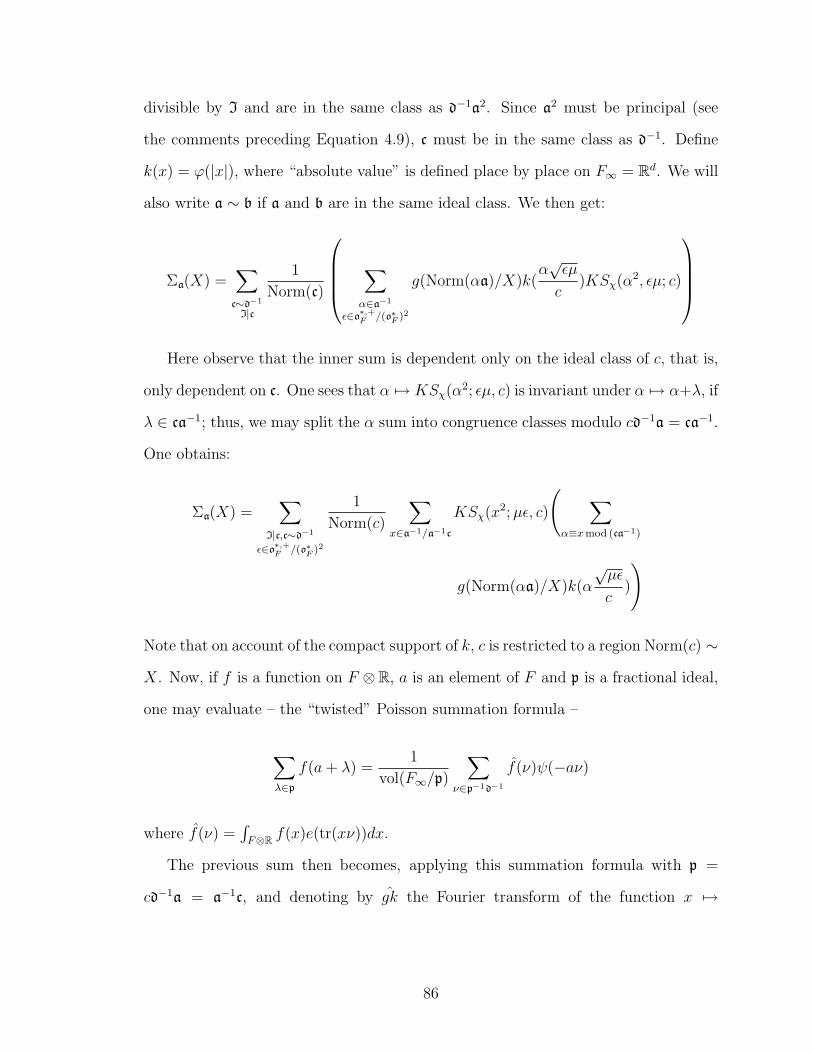
divisible by I and are in the same class as d−1a2. Since a2 must be principal (see
the comments preceding Equation 4.9), c must be in the same class as d−1. Define
k(x) = ϕ(|x|), where “absolute value” is defined place by place on F∞ = Rd. We will
also write a ∼ b if a and b are in the same ideal class. We then get:
Σa(X) =∑
c∼d−1
I|c
1
Norm(c)
∑α∈a−1
ε∈o∗,+F /(o∗F )2
g(Norm(αa)/X)k(α√εµ
c)KSχ(α
2, εµ; c)
Here observe that the inner sum is dependent only on the ideal class of c, that is,
only dependent on c. One sees that α 7→ KSχ(α2; εµ, c) is invariant under α 7→ α+λ, if
λ ∈ ca−1; thus, we may split the α sum into congruence classes modulo cd−1a = ca−1.
One obtains:
Σa(X) =∑
I|c,c∼d−1
ε∈o∗,+F /(o∗F )2
1
Norm(c)
∑x∈a−1/a−1c
KSχ(x2;µε, c)
( ∑α≡xmod (ca−1)
g(Norm(αa)/X)k(α
√µε
c)
)
Note that on account of the compact support of k, c is restricted to a region Norm(c) ∼
X. Now, if f is a function on F ⊗R, a is an element of F and p is a fractional ideal,
one may evaluate – the “twisted” Poisson summation formula –
∑λ∈p
f(a+ λ) =1
vol(F∞/p)
∑ν∈p−1d−1
f(ν)ψ(−aν)
where f(ν) =∫F⊗R f(x)e(tr(xν))dx.
The previous sum then becomes, applying this summation formula with p =
cd−1a = a−1c, and denoting by gk the Fourier transform of the function x 7→
86

g(Norm(xa)/X)k(√µεx/c):
∑I|c,c∼d−1
ε∈o+F /(o
∗F )2
1
Norm(c)vol(F∞/cd−1a)
∑ν∈a−1
gk(νc−1)∑
x∈a−1/a−1c
KSχ(x2;µε, c)ψ(−νx
c)
(4.13)
Now
gk(νc−1) =
∫F∞
g(Norm(x)Norm(a)
X)k(
√µε
cx)ψ(xν/c)dx (4.14)
= Norm(c)
∫F∞
g(Norm(x)Norm(ac)
X)k(√µεx)ψ(xν)dx (4.15)
Define Ψc,ε(ν) as follows:
Ψc,ε(ν) =
∫F∞
g(Norm(x)Norm(ac)/X)k(√µεx)ψ(xν)dx
and define Aa(ν; c, µε) =∑
x∈a−1/a−1cKSχ(x2, µε, c)ψ(−νx
c), the local sum that occurs
in Equation 4.13. This sum is analyzed in the next two sections, and the results
relevant to us are summarized in Proposition 12 and Corollary 2; we will continue
assuming the results from there.
We substitute into Equation 4.13 the definitions of Ψc,ε, Aa and the fact that
vol(F∞/oF ) = D1/2F . Then:
Σa(X) =D
1/2F
Norm(a)
∑I|c,c∼d−1
ε∈o∗,+F /(o∗F )2
(∑ν∈a−1
Aa(ν; c, µε)
Norm(c)Ψc,ε(ν)
)(4.16)
Fix a norm || · || on F∞, considered as an R-vector space. Now, the function
Ψc,ε is the Fourier transform of a function of compact support and with reasonable
derivatives, so it decays rapidly, uniformly in c for Norm(c) ∼ X. That is, it will
satisfy a uniform estimate Ψc,ε(ν) X||ν||−M . By an argument parallel to that of
Chapter 2, one sees that the double sum above is absolutely convergent, and it is
87

possible to truncate the above sum to ||ν|| Xδ, for any δ > 0 (but δ fixed as
X → ∞.) As in Chapter 2, only certain values of ν will contribute in the limit;
namely, those ν such that inner sum of Equation 4.16 does not manifest cancellation.
Expanding Ψc,ε(ν), we may write Equation 4.16 as:
Σa(X) =D
1/2F
Norm(a)
∑ν∈a−1
ε∈o∗,+F /(o∗F )2
∫F⊗R
k(x√µε)ψ(xν) (4.17)
∑I|c,c∼d−1
g(Norm(x)Norm(ca)
X)Aa(ν; c, µε)
Norm(c)
dx (4.18)
The following Proposition expresses the behavior of the innermost “local sum”
above. It may be deduced from Corollary 2 of the next section.
Proposition 11. Let C be the constant defined in Proposition 12. Recall the defini-
tion of the set of “twisted fields” S from Section 4.3.1, and recall that S is identified
with a set of classes in F ∗/(F ∗)2, whence it is meaningful to ask whether an element
of F lies in S . Note that |S| = |CF (2)|, the cardinality of the 2-torsion in CF . Fix
a norm || · || on F∞. Fix a ∈ A. For x ∈ F , define
δa(x) =
h−1F C x 6= 0, x ∈ Ia−2, x ∈ S;
|CF (2)|2
h−1F C x = 0;
0 else
Then, for α ∈ R, for some A > 0, and for all ε > 0,
∑I|c,c∼d−1
g(Norm(c)α
X)Aa(ν; c, µ)
Norm(c)= δa(ν
2 − 4µ)X
α+Oε((1 + ||ν||)A(X/α)1/2+ε)
Applying this with α = DFNorm(a)−1Norm(x), and using the assumption that
k is compactly supported, and the fact, remarked after Equation 4.16, that we can
88

truncate the ν-sum to ||ν|| Xδ, we obtain:
Σa(X) = D−1/2F X
∑ν∈a−1
ε∈o∗,+F /(o∗F )2
δa(ν2−4µε)
∫F⊗R
k(x√µε)
1
Norm(x)ψ(xν)dx+Oε(X
1/2+ε)
(4.19)
Now∫F⊗R k(x
√µε) 1
Norm(x)ψ(xν)dx = ∆( ν√
µε), where ∆ is the Fourier transform of
k(x)/Norm(x). We would also like an arithmetic parameterization of ν such that
δa(ν2 − 4µε) 6= 0; this is given by the
Lemma 7. Fix µ ∈ a−2. Let S = (x,K), K ∈ S, x ∈ a−1oK,I, NormK/F (x) = µ,
where oK,I is the order of K defined at the start of Subsection 4.3.3, and let S′ =
ν ∈ a−1 : δa(ν2 − 4µ) 6= 0. Then there is a map S → S′, given by x 7→ trK/F (x),
which is surjective; the fibre above ν has size 2 unless ν2 = 4µ, in which case it has
size |S| = |CF (2)|.
Proof. This is not entirely formal, but straightforward, and we omit the details.
Equation 4.19 becomes:
limX→∞
Σa(X)
X=h−1F D
−1/2F C
2
∑K∈S
∑ε∈o∗,+
F /(o∗F )2
∑x∈a−1oK,I:NormK/F (x)=µε
∆(trK/F (x)√µε
)
(4.20)
We transfer this to a statement in terms of h, using the transformation formula
Equation 4.8. We need to first fix a notation.
For each K ∈ S, let σK be the nontrivial Galois automorphism of K over F . For
each place v of F , let τv be the corresponding embedding of F into R and choose
an embedding σv of K into R extending τv. Then, for x ∈ K, define log(x) =
(log(|σv(x)/σKσv(x)|))v, an element of R[F :Q]. This is perhaps not the most obvious
choice for the meaning of log; the point of this definition is that it is trivial for x ∈ F .
Also note that a different choice of σv changes the sign of some co-ordinates; this will
be irrelevant. Using Equation 4.8 and some manipulation we find that, for x ∈ K
89

with NormK/F (x) = µε,
∆(trK/F(x)√µε
) = 2[F :Q]−1h(1
2πlog(x)) (4.21)
It is convenient (for the eventual purpose of matching trace formulae) to make
a further translation of the result. We define o′K,I to be the elements of oK,I with
norm in o∗,+F . Note that o∗F ⊂ o′K,I. Let XK,a,(µ) be a set of representatives, modulo
the action of o′K,I, for elements x0 ∈ a−1oK,I with totally positive norm and so that
(NormK/F (x0)) = (µ), i.e. NormK/F (x0) = µε for some ε ∈ o∗,+F .
One now obtains:
limX→∞
Σa(X)
X= 2[F :Q]−2h−1
F D−1/2F C
∑K∈S
∑x∈XK,a,(µ)
∑ε′∈o
′K,I/o
∗F
h(1
2πlog(xε′))
(4.22)
This expression is valid even if m is not principal.
We finally sum over ideals a according to Equation 4.10 in order to recover Σ(X).
We therefore set, for a ∈ A, XK,a,m to be a set of representatives, modulo the action
of o′K,I, for elements x0 ∈ a−1oK,I with totally positive norm and generating a−2m.
Then
L = limX→∞
Σ(X)
X= 2[F :Q]−2h−1
F D−1/2F C
∑K∈S
∑a∈A
∑x∈XK,a,m
∑ε′∈o
′K,I/o
∗F
h(1
2πlog(xε′))
(4.23)
To make the expression look somewhat nicer, we now introduce the constant:
VI = 22−[F :Q]hFD3/2F ζ(F, 2)Norm(I)
∏q|I
(1 + Norm(q)−1)
which is, up to a constant bounded in terms of [F : Q], the volume of the space
qa∈AXa. (This is with respect to the normalization of measure defined in the Ap-
90

pendix.) Recall also the definition of Cf (after Remark 8), so that af (a, α) =
Cfλf (aαd).
Finally, note that (for any K ∈ S) the absolute discriminant of oK,I is given by
Disc(oK,I) = D2FNorm(I); we denote it by DK,I. Therefore
√Norm(I) =
√DK,ID
−1F .
It is also worth noting that one expects |Cf |2 to be of size about√DF
VI. (This is not a
simple consequence of anything stated so far. We state it as a fact so the reader has
more feeling for the order of magnitude of the quantities.)
With some manipulation, we obtain the final answer, phrased in terms of Hecke
coefficients:
limX→∞
(∑f hf (ϕ)|Cf |2λf (m)
∑q g(Norm(q)/X)λf (q
2) + C.S.C∑q g(Norm(q)/X)
)
=
√DF
VI
√DK,I
DF
∑K∈S
∑a∈A
x∈XK,a,m
∑ε′∈o
′K,I/o
∗F
h(1
2πlog(xε′))
(4.24)
4.4 Computation of the local sums
The aim of this section is to evaluate the local sums that arose in the previous section.
The results of this section were already used in the derivation of the limit formula
Equation 4.24.
4.4.1 Translation of local sums to adelic integrals
The local sums that have been encountered in Equation 4.13 will be most conveniently
expressed (and evaluated) in terms of adelic integrals; that is the purpose of what
follows. This will make clear the multiplicativity, and, more importantly, makes
more clear (at least to me) what happens at bad places, such as those dividing 2.
Unfortunately, there will be a considerable notational burden in this section; it seems
unavoidable.
91

We will continue to assume that χ is the Grossencharacter associated to the totally
real quadratic extension K0 over F . We use, as before χf for the induced character
of (oF/fχ)× obtained by restricting χ to elements of A×
F,f that are of valuation 0
everywhere; occasionally, when it is clear, we will merely use χ in this case. Note
that, since K is totally real, χ is trivial on F×∞ (although we indicate at the point
where this is used how it can be removed).
Fix a ∈ A, ν ∈ a−1, µ ∈ a−2. c will be an element of Ia−1, and we continue
with the notational convention introduced at the start of Subsection 4.3.4, namely, c
denotes the ideal d−1a2(c).
We then wish to analyze the sum
Aa(ν; c, µ) =∑
m∈a−1/a−1c
KSχ(m2, µ; c)ψ(−mν
c) (4.25)
=∑
x∈(o/c)×
∑m∈a−1/a−1c
ψ(m2x+ µx−1 −mν
c)χf (x)
=∑
x∈(o/c)×
∑m∈a−1/a−1c
ψ(x−1m2 + µ−mν
c)χf (x)
The sums may be replaced by integrals over oF , the completion of oF with respect
to ideals; it is the maximal compact subring of AF,f , or, in other words, the product∏v finite oF,v. The group of units o×F is the product
∏v finite o×F,v. Let πa be an idele
corresponding to a. We obtain–using measures that assign mass 1 to the domains
of integration, which we denote by d(1), denoting by φ(c) the “Euler phi” function
|(o/c)×|, and considering χf as a character on o×F ⊂ A×F ,
Aa(ν; c, µ) = Norm(c)φ(c)
∫x∈o×F
∫m∈π−1
a oF
ψ(x−1m2 + µ−mν
c)χf (x)d
(1)xd(1)m
We may, since χ is trivial on F×∞ ⊂ A×
F , harmlessly insert a factor χf (c). (Note
this insertion would in fact be valid in general, since the definition of the Kloosterman
92

sum, in the Equation 4.50 derived at the end of this Chapter, involves a factor χ∞(c).)
For A,B ∈ A×F,f , we write (A) = (B) if the associated fractional ideals are equal, that
is, AB−1 ∈ o×F . With this notation:
Aa(ν; c, µ) = Norm(c)φ(c)
∫z∈A×F,f ,(z)=(c)
∫m∈π−1
a oF
ψ(z−1(m2 −mν + µ)χ(z)d(1)zd(1)m
Since χ is quadratic, χ(π2a) = 1, so:
Aa(ν; c, µ) = Norm(c)φ(c)
∫(z)=(cπ2
a)
∫m∈oF
ψ(z−1(m2 −mπaν + π2aµ)χ(z)d(1)zd(1)m
This motivates the definition of the adelic integral.
Definition 5. Let c′ be any ideal divisible by d, and ν ′, µ′ ∈ AF . We define I(ν ′; c′;µ′)
to be this integral:
Norm(c′d−1)φ(c′d−1)
∫(z)=c′
∫m∈oF
ψ(z−1(m2 −mν ′ + µ′))χ(z)d(1)zd(1)m (4.26)
where the measures are Haar measures that assign mass 1 to the domain of integration.
Note that ν ′ and µ′ do not have to be elements of F . Also note that we will only ever
apply this where the ideal c′ “contains” the ramification of both χ and ψ; we do not
need to make this precise for now.
Therefore, the sum Aa(ν; c, µ) defined in Equation 4.25 is related by Aa(ν; c, µ) =
I(νπa; cd, µπ2a) – where, as throughout, we are using the convention that c = d−1a2(c).
Note that it is invariant under (ν, µ) → (νu, µu2) for u ∈ oF×.
4.4.2 Zeta functions
To understand the average behavior of Aa(ν; c, µ) with respect to c, we introduce a
“zeta series”, or, at least one for the corresponding integral I. It is defined in Defini-
93

tion 6, and the relation to I is clarified in Lemma 8; the main result is Proposition
12, and we finally translate back to the local sum Aa(ν; c, µ) in Corollary 2. The bulk
of the proof of the Proposition is contained in the next Subsection.
We will fix ν ′, µ′ ∈ A×F so that there exist elements ν0, µ0 ∈ F× and ι ∈ A×
F so
that ν ′ = ν0ι, µ′ = µ0ι
2. This is, in particular, the case needed to apply the results
to Aa(ν; c, µ) = I(νπa; cd, µπ2a). In particular, one can speak of F (
√ν ′2 − 4µ′): by
it we mean the quadratic field F (√ν2
0 − 4µ0), or equivalently the unique quadratic
extension of F which, for every place v of F , agrees with Fv(√ν ′2v − 4µ′v). (As usual,
by ν ′v we mean the component at v of the adele ν ′; it is thus an element of Fv.) For a
finite place v, by v(ν ′2 − 4µ′) we mean the valuation v(ν ′2v − 4µ′v). We also note that
if ν ′2 − 4µ′ is zero at one place it is zero everywhere.
We now introduce the zeta series. Lemma 8 and Equation 4.28 will make concrete
the relation between I and this zeta function. We also use ν ′, µ′ for the arguments of
I to continue to emphasize that they need not lie in the field F , but only in AF .
It is also convenient to make this definition of the zeta-function for an arbitrary
Grossencharacter ω. It will eventually be applied for ω an unramified twist of the
original χK0 .
For each finite place v, fix Haar measure dx on Fv so that the measure of ov is
1, and define measure on F×v so that the measure of o×v is (1 − q−1
v ). With these
normalizations:
Definition 6. Let ω be a Grossencharacter of A×F/F
× (not necessarily quadratic).
Let ωv, ψv be the restrictions of the Grossencharacter ω and the additive character ψ
to Fv. We define the local factor Zv(ωv, s) via:
Zv(ωv, s) =∑r≥v(I)
Zv,rqr(1−s)v (4.27)
94

where for r ≥ 0 integral,
Zv,r =
∫v(x)=r+v(d)
∫m∈oF,v
ψv(x−1(m2 −mν ′ + µ′))ωv(x)dxdm, r ≥ 1
1(1−q−1
v )
∫v(x)=v(d)
∫m∈oF,v
ψv(x−1(m2 −mν ′ + µ′))ωv(x)dxdm, r = 0
Finally, we define:
Z(ω, s) =∏v finite
Zv(ωv, s)
Note that Zv,0 = 0 unless ω is unramified; in that case, it equals ω(dv).
The following Lemma is now an easy consequence of the definitions.
Lemma 8. With this definition,
∑I|c
I(ν ′; cd, µ′)Norm(c)−1−s = Z(χK0 , s)
We are interested (see Proposition 11) in the behavior ofAa(ν; c, µ) = I(νπa; cd, µπ2a)
when c ∼ d−1. Therefore, we use characters of CF to “pick out” the ideal class of the
different:
∑I|c,c∼d−1
I(ν ′; cd, µ′)
Norm(c)Norm(c)−s =
1
hF
∑χ′∈CF
χ′(d)
∑I|c
I(ν ′; dc, µ′)
Norm(c)Norm(c)−sχ′(c)
=
1
hF
∑χ′∈CF
Z(χχ′, s) (4.28)
We summarize the results we will prove about Z(ω, s) in the following Proposition.
Note it is important to separate the case ν ′2 − 4µ′ = 0. The results are true in
a good deal more generality than that in which we state them; we restrict ourself
considerably for ease of proof.
Proposition 12. Let ω be an unramified twist of χK0 (such as occurs in Equation
4.28), so ω = χK0χ′ for χ′ ∈ CF .
95

The function Z(ω, s) extends to a meromorphic function on the complex plane.
Let χν′2−4µ′ be the Grossencharacter of F that is associated to the quadratic extension
F (√ν ′2 − 4µ′).
Suppose ν ′2 − 4µ′ 6= 0. Then Z(ω, s) is analytic for <(s) > 1/2, unless ωχν′2−4µ′
is trivial and I|ν ′2 − 4µ′ (that is, for each finite valuation, v(ν ′2 − 4µ′) ≥ v(I)). In
that case, it has just one pole for <(s) > 1/2, at s = 1, and that is a simple pole with
residue:
Ress=1Z(ω, s) = C ≡ ress=1ζ(F, s)
ζ(F, 2)√
Norm(I)∏
q|I(1 + Norm(q)−1)(4.29)
Suppose ν ′2 − 4µ′ = 0. Then Z(ω, s) is analytic for <(s) > 1/2, unless ω is
quadratic. In that case, it has just one pole for <(s) > 1/2, which is at s = 1, and it
is a simple pole with residue 12C, where C is as above.
In all cases, the function Z(s) has slow growth along vertical strips for <(s) > 1/2:
if σ > 1/2, one has an estimate: |Z(σ+ it)| (1 + ||ν ′||AF)A(σ)(1 + |t|)B(σ), for some
appropriate A(σ), B(σ).
Proof. (Borrowed from upcoming section): contained in Corollary 3 and Equation
4.38.
Using Equation 4.28 and the relation between Aa(ν; c, µ) and the adelic integral
I, we obtain:
Corollary 2. The sum∑
I|c,c∼d−1 Aa(ν; c, µ)Norm(c)−1−s is meromorphic, with at
most a pole at s = 1 in the half-plane <(s) > 1/2, and it has a pole at s = 1 only
if ν2 − 4µ ∈ S and ν2 − 4µ ∈ Ia−2. (Here S is as in Subsection 4.3.1.) If C is the
constant of Equation 4.29, the residue at s = 1 is given by:
h−1F C, ν2 − 4µ 6= 0
|CF (2)|2
h−1F C, ν2 − 4µ = 0
96
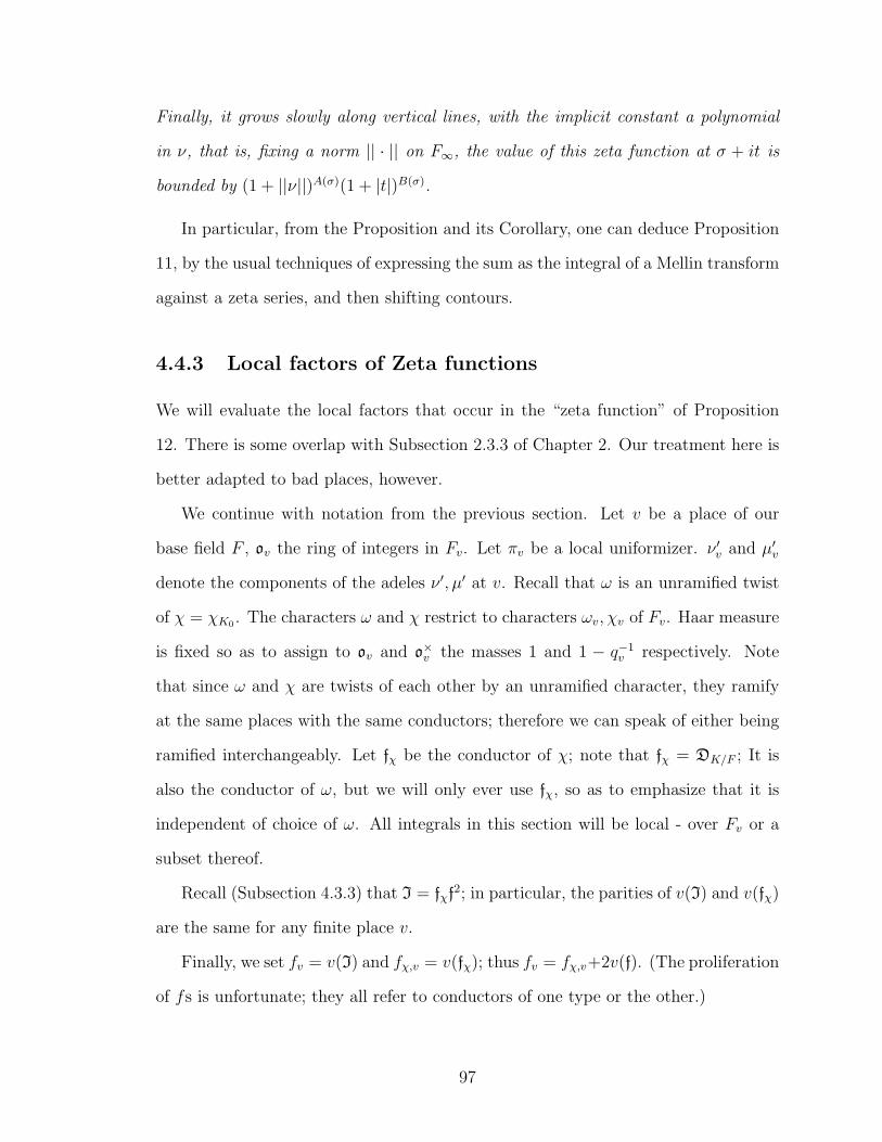
Finally, it grows slowly along vertical lines, with the implicit constant a polynomial
in ν, that is, fixing a norm || · || on F∞, the value of this zeta function at σ + it is
bounded by (1 + ||ν||)A(σ)(1 + |t|)B(σ).
In particular, from the Proposition and its Corollary, one can deduce Proposition
11, by the usual techniques of expressing the sum as the integral of a Mellin transform
against a zeta series, and then shifting contours.
4.4.3 Local factors of Zeta functions
We will evaluate the local factors that occur in the “zeta function” of Proposition
12. There is some overlap with Subsection 2.3.3 of Chapter 2. Our treatment here is
better adapted to bad places, however.
We continue with notation from the previous section. Let v be a place of our
base field F , ov the ring of integers in Fv. Let πv be a local uniformizer. ν ′v and µ′v
denote the components of the adeles ν ′, µ′ at v. Recall that ω is an unramified twist
of χ = χK0 . The characters ω and χ restrict to characters ωv, χv of Fv. Haar measure
is fixed so as to assign to ov and o×v the masses 1 and 1 − q−1v respectively. Note
that since ω and χ are twists of each other by an unramified character, they ramify
at the same places with the same conductors; therefore we can speak of either being
ramified interchangeably. Let fχ be the conductor of χ; note that fχ = DK/F ; It is
also the conductor of ω, but we will only ever use fχ, so as to emphasize that it is
independent of choice of ω. All integrals in this section will be local - over Fv or a
subset thereof.
Recall (Subsection 4.3.3) that I = fχf2; in particular, the parities of v(I) and v(fχ)
are the same for any finite place v.
Finally, we set fv = v(I) and fχ,v = v(fχ); thus fv = fχ,v+2v(f). (The proliferation
of fs is unfortunate; they all refer to conductors of one type or the other.)
97

The local factor of the zeta function that we are interested in has been defined in
Equation 4.27.
Evaluation at good places
We begin by evaluating at “good” places. Recall that χν′2−4µ′ is the quadratic char-
acter associated with the extension F (√ν ′2 − 4µ′) – by definition, we take it to be
trivial if ν ′2 − 4µ′ is a square.
Lemma 9. For almost all places v,
Zv(ω, s) =
1 + ωv(πv)χν′2−4µ′(πv)q
−sv =
Lv(s,ωχν′2−4µ′ )
Lv(2s,ω2v)
, ν ′2 − 4µ′ 6= 0
Lv(2s−1,ω2v)
Lv(2s,ω2v), ν ′2 − 4µ′ = 0
(4.30)
Here Lv is the factor at v of the Hecke-Tate L-function.
Proof. This follows as in Chapter 2, Subsection 2.3.3.
As a Corollary we obtain part of Proposition 12:
Corollary 3. Z(ω, s) extends to a meromorphic function of s, analytic in <(s) > 1/2.
It does not have a pole at s = 1 unless either:
1. ν ′2 − 4µ′ 6= 0 and ωχν′2−4µ′ is the trivial character, or:
2. ν ′2 − 4µ′ = 0 and ω is quadratic.
Finally, it has a growth bound of the form |Z(σ+ it, ω)| (1 + ||ν||)A(σ)(1 + |t|)B(σ).
Proof. (Sketch) The conclusion is clearly true for the product over almost all v, and
one must check, as in Chapter 2, that the finite number of bad factors do not jeop-
ardize the conclusion. The only difficulty is at primes above 2, and even then it is
easily verified by the methods developed in the rest of this Subsection.
98
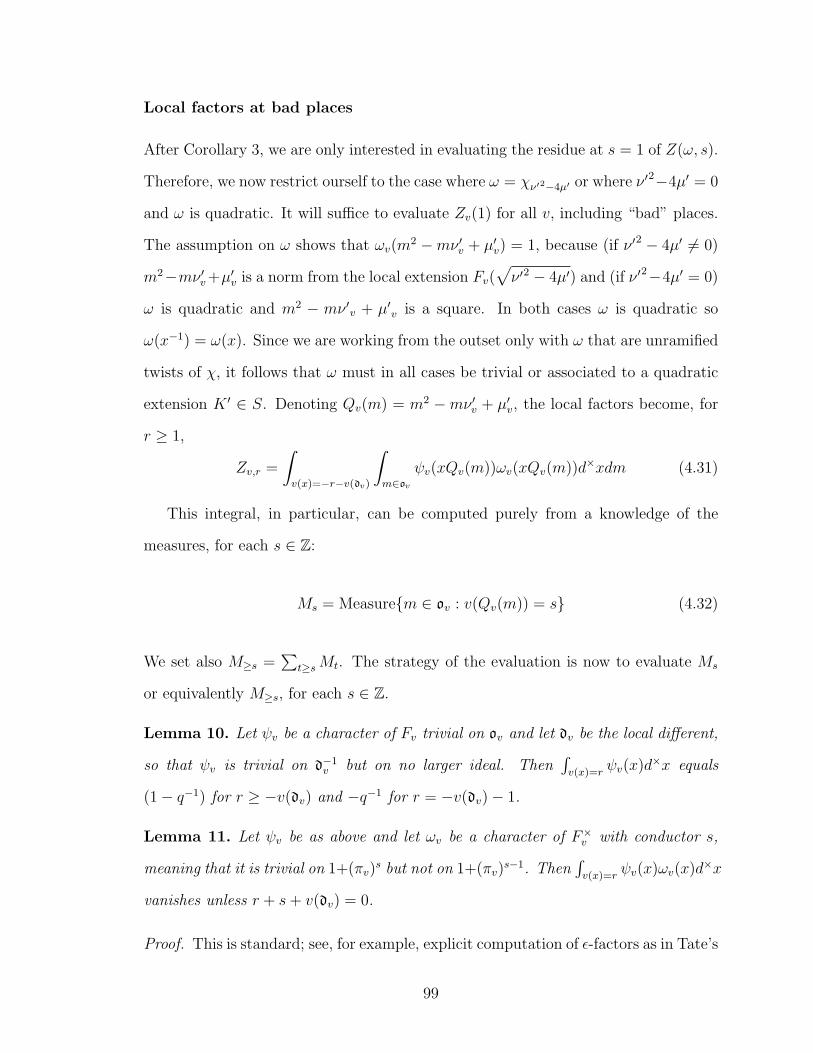
Local factors at bad places
After Corollary 3, we are only interested in evaluating the residue at s = 1 of Z(ω, s).
Therefore, we now restrict ourself to the case where ω = χν′2−4µ′ or where ν ′2−4µ′ = 0
and ω is quadratic. It will suffice to evaluate Zv(1) for all v, including “bad” places.
The assumption on ω shows that ωv(m2 −mν ′v + µ′v) = 1, because (if ν ′2 − 4µ′ 6= 0)
m2−mν ′v+µ′v is a norm from the local extension Fv(√ν ′2 − 4µ′) and (if ν ′2−4µ′ = 0)
ω is quadratic and m2 − mν ′v + µ′v is a square. In both cases ω is quadratic so
ω(x−1) = ω(x). Since we are working from the outset only with ω that are unramified
twists of χ, it follows that ω must in all cases be trivial or associated to a quadratic
extension K ′ ∈ S. Denoting Qv(m) = m2 −mν ′v + µ′v, the local factors become, for
r ≥ 1,
Zv,r =
∫v(x)=−r−v(dv)
∫m∈ov
ψv(xQv(m))ωv(xQv(m))d×xdm (4.31)
This integral, in particular, can be computed purely from a knowledge of the
measures, for each s ∈ Z:
Ms = Measurem ∈ ov : v(Qv(m)) = s (4.32)
We set also M≥s =∑
t≥sMt. The strategy of the evaluation is now to evaluate Ms
or equivalently M≥s, for each s ∈ Z.
Lemma 10. Let ψv be a character of Fv trivial on ov and let dv be the local different,
so that ψv is trivial on d−1v but on no larger ideal. Then
∫v(x)=r
ψv(x)d×x equals
(1− q−1) for r ≥ −v(dv) and −q−1 for r = −v(dv)− 1.
Lemma 11. Let ψv be as above and let ωv be a character of F×v with conductor s,
meaning that it is trivial on 1+(πv)s but not on 1+(πv)
s−1. Then∫v(x)=r
ψv(x)ωv(x)d×x
vanishes unless r + s+ v(dv) = 0.
Proof. This is standard; see, for example, explicit computation of ε-factors as in Tate’s
99

thesis.
With ωv, ψv as in Lemma 11, we denote the value of∫v(x)=−s−v(dv)
ψv(x)ωv(x)d×x
by g(ωv, ψv). It has absolute value qs/2.
Definition 7. Suppose ωv is ramified at v. We denote by ε(ωv, ψv) the “sign” g(ωv ,ψv)|g(ωv ,ψv)| .
If ψv is ramified at v, i.e. v(d) 6= 0, but ωv is not, we let ε(ωv, ψv) = ωv(dv).
Finally, if neither ψv or ωv are ramified, we set ε(ωv, ψv) = 1.
Lemma 12. The product∏
v finite ε(ωv, ψv) equals 1.
Proof. ω is, as remarked, associated to a quadratic field K ′ ∈ S. The Lemma follows
by computing the root numbers for the L-functions L(K ′, s) and L(F, s); the εv are
essentially the local root numbers for their quotient. Standard computations and the
fact that K ′ is unramified at ∞, that is to say, totally real, give the result.
It follows from the definitions that, if we set ωv(dv) = 0 when ωv is ramified:
Zv(1) =
∑
r≥v(I) Zv,r, v(I) ≥ 1
ω(dv) +∑
r≥1 Zv,r, v(I) = 0
Let k ≥ 1 be an integer. We see that, with Ms as in Equation 4.32:
∑r≥k
Zv,r =∑t∈Z
r≤−k−v(dv)
Mt
∫v(x)=r+t
ψv(x)ωv(x)d×(x) (4.33)
=∑s∈Z
∫v(x)=s
ψv(x)ωv(x)∑
t≥s+k+v(dv)
Mt (4.34)
Recall the definitions v(I) = fv, v(fχ) = fχ,v. We distinguish now three cases:
1. If ωv is ramified with conductor fχ, the only contribution to the above integral
100

is when s+ fχ,v + v(dv) = 0. It follows that, by Lemma 11,
Zv(1) = g(ωv, ψv)∑
t≥fv−fχ,v
Mt = g(ωv, ψv)M≥fv−fχ,v (4.35)
2. Suppose ωv is unramified and nontrivial. Then by Lemma 10,
Zv(1) =
(−1)v(dv)
(q−1v M≥fv−1 + (1− q−1
v )∑
s≥fv(−1)s−fvM≥s
), fv ≥ 1
(−1)v(dv)(1 + q−1
v M≥0 + (1− q−1v )∑
s≥1M≥s), fv = 0
(4.36)
3. If ωv is trivial, then
Zv(1) = −q−1M≥fv−1 + (1− q−1)
∑s≥fv
M≥s, fv ≥ 1
Zv(1) = 1− q−1M≥0 + (1− q−1)∑
s≥1M≥s fv = 0
(4.37)
4.4.4 Evaluation of measures and of zeta functions
Let, as before, v be a finite place of F , and Qv as defined prior to Equation 4.31. The
aim of this section is to compute the measures Ms = Measurem ∈ ov : v(Qv(m)) =
s, or equivalently M≥s =∑
t≥sMt, for each t; this will then complete our evaluation
of local factor Zv(1) by the formulas 4.35, 4.36 and 4.37 of the last section. Again,
the answer depends on the splitting type of the quadratic form Qv(m). We will list
the evaluation of the measures and also give, in each case, the parity of the constants
fχ,v, fv and v(ν ′2 − 4µ′); it will then be easy to deduce Zv(1). (Recall the definitions
of fχ,v and fv from Subsection 4.4.3.)
If ν ′ is (locally) divisible by 2, we can complete the square: m2 − mν ′v + µ′v =
(m−ν ′v/2)2 +(µ′v−ν ′v2/4). Therefore Qv(m) is equivalent to the form q(x) = x2−β,
with β = ν ′v2 − µ′v/4. If the residue characteristic is 2, we must proceed slightly
differently.
101

1. Non-split case, residue characteristic 6= 2: By “non-split” we mean that β =
ν ′v2 − µ′v/4 is not a square; equivalently, the local extension Fv(
√ν ′v
2 − 4µ′v) is
not split. Then, if v(x) < v(β)/2, then v(q(x)) = 2v(x); if v(x) ≥ v(β)/2, then
v(q(x)) = v(β). Also v(β) = v(ν ′2 − 4µ′), as the residue characteristic is not 2.
Thus M≥s = q−ds/2ev for s ≤ v(ν ′2 − 4µ′), and M≥s = 0 for s > v(ν ′2 − 4µ′).
We divide into two further subcases:
(a) Ramified: In this case Zv(1) is, by Equation 4.35, g(ωv, ψv)M≥f−fχ . In this
case fχ,v = 1, v(ν ′2− 4µ′) is odd, and fv = v(I) is odd as fv ≡ fχ,v mod 2.
(b) Nonramified: In this case Zv(1) is given by Equation 4.36; fχ,v = 0, and
both fv and v(ν ′2 − 4µ′) are even.
2. Nonsplit case, residue characteristic = 2:
Write Qv(m) = (m − β1)(m − β2). Here β1, β2 are conjugate elements of the
quadratic extension defined by Qv, and (β1−β2)2 = ν ′2v− 4µ′v. Also v(Q(m)) =
2v(m− β1), for m ∈ Fv.
LetKQ be the quadratic extension of Fv defined byQv, that is, the field obtained
by adjoining β1. We denote ov by oF,v so as to clearly distinguish between Fv
and KQ. Extend the valuation to KQ; it may now take non-integral values.
Let πF,v and πK be uniformizers for Fv and KQ respectively. We can choose
x ∈ oKQso that oKQ
= oF,v ⊕ xoF,v. The local discriminant is then given by
(x − xσ)2, where σ is the Galois automorphism. If KQ is unramified, then we
can take πK = πF,v, and oKQ/πlKoKQ
= oF,v/πlF,voF,v ⊕ xoF,v/π
lF,voF,v.
If KQ is ramified over Fv, then we still have oKQ/π2l
KoKQ= oF,v/π
lF,voF,v ⊕
xoF,v/πlF,voF,v. If an element of oKQ
is congruent to an element of oF,v mod
π2lK , it is automatically so modulo π2l+1
K ; this is essentially a consequence of the
isomorphism oF,v/πF,voF,v → oKQ/πKoKQ
.
102
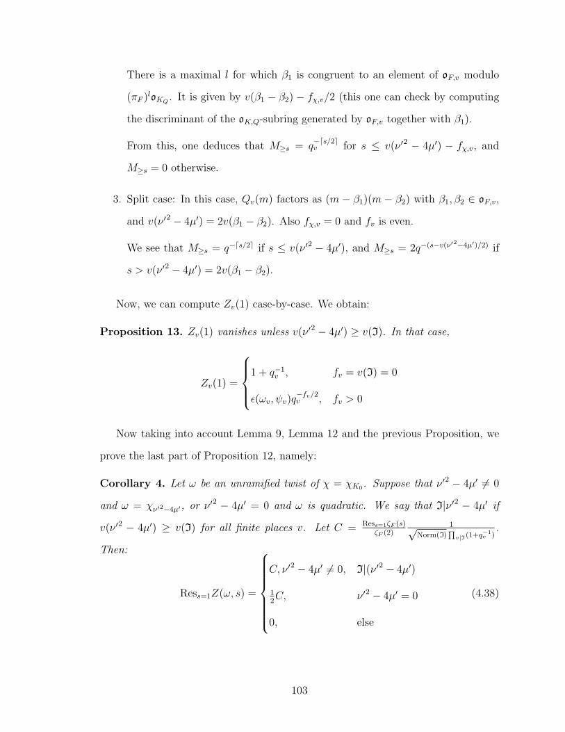
There is a maximal l for which β1 is congruent to an element of oF,v modulo
(πF )loKQ. It is given by v(β1 − β2) − fχ,v/2 (this one can check by computing
the discriminant of the oK,Q-subring generated by oF,v together with β1).
From this, one deduces that M≥s = q−ds/2ev for s ≤ v(ν ′2 − 4µ′) − fχ,v, and
M≥s = 0 otherwise.
3. Split case: In this case, Qv(m) factors as (m − β1)(m − β2) with β1, β2 ∈ oF,v,
and v(ν ′2 − 4µ′) = 2v(β1 − β2). Also fχ,v = 0 and fv is even.
We see that M≥s = q−ds/2e if s ≤ v(ν ′2 − 4µ′), and M≥s = 2q−(s−v(ν′2−4µ′)/2) if
s > v(ν ′2 − 4µ′) = 2v(β1 − β2).
Now, we can compute Zv(1) case-by-case. We obtain:
Proposition 13. Zv(1) vanishes unless v(ν ′2 − 4µ′) ≥ v(I). In that case,
Zv(1) =
1 + q−1
v , fv = v(I) = 0
ε(ωv, ψv)q−fv/2v , fv > 0
Now taking into account Lemma 9, Lemma 12 and the previous Proposition, we
prove the last part of Proposition 12, namely:
Corollary 4. Let ω be an unramified twist of χ = χK0. Suppose that ν ′2 − 4µ′ 6= 0
and ω = χν′2−4µ′, or ν ′2 − 4µ′ = 0 and ω is quadratic. We say that I|ν ′2 − 4µ′ if
v(ν ′2 − 4µ′) ≥ v(I) for all finite places v. Let C = Ress=1ζF (s)ζF (2)
1√Norm(I)
∏v|I(1+q−1
v ).
Then:
Ress=1Z(ω, s) =
C, ν ′2 − 4µ′ 6= 0, I|(ν ′2 − 4µ′)
12C, ν ′2 − 4µ′ = 0
0, else
(4.38)
103

4.5 Expected answer
Here we sketch the expected answer, that is, the answer we expect when we assume
that dihedral forms arise from Grossencharacters of quadratic field extensions K. As
in Chapter 2, the matching of this expected answer with what we derived (in Equation
4.23 or Equation 4.24) leads formally to the classification of dihedral forms.
One expects:
Expectation 1. Automorphic forms π on GL(2) over F , such that L(s, π, Sym2) has
a pole, correspond to Grossencharacters ω of quadratic K/F so that the restriction
of ω to AF is trivial; the correspondence is specified by the matching of L-functions.
We will denote by π(ω) the GL(2)-form on F associated to the K-Grossencharacter
ω. The conductor of π(ω) is given by DK/FNorm(fω), where fω is the conductor of ω.
In particular, if J is a prime ideal of F prime to any ramification of K or ω, then
the Jth Hecke coefficient of π(ω) is given by:
λJ(π(ω)) =∑
B:Norm(B)=J
ω(B) (4.39)
As before, we have fixed a totally real quadratic extension K of F , and an integral
ideal I = DK/F f2 of F . It determines an order oK,I of K by oF + foK ; this is a subring
of oK . For each finite valuation v of K, we set UI,v to be the units (elements of
valuation 0) in the closure of oK,I in Kv. We set UI =∏
v UI,v; it is an open compact
subgroup of A×K,f (the ring of finite ideles of K.) Since I is fixed, we wil often refer
to UI simply as U .
One sees that:
Lemma 13. Let ω be a character of A×K/K
×A×F . Then the conductor of ω is the
extension of an F -ideal; and it has conductor dividing (f)K (the extension of f to K)
if and only if it is trivial on UI. In particular, one expects π such that L(s, π, Sym2)
104

has a pole and Conductor(π)|I to correspond to characters of A×K/K
×A×FUI.
We are therefore interested in making explicit the structure of A×K/K
×A×FU . It is
convenient, as it turns out, to work out the structure of A×K/K
×F×∞U and then “take
the quotient by A×F at the end.” The notation is, unfortunately, rather unwieldy, and
we introduce it all now just for a convenient reference.
Notation: Let ΛU be the set of U -units of K, that is to say, elements of K that
are in U at every finite place; equivalently, this is the set of units in the order oK,I.
We also define Λ′U to be the intersection K ∩ (U ·A×
F ); equivalently, this is the set of
elements λ ∈ K that generate an oK,I-ideal that is the extension of an ideal of F .
We also introduce notation for the class groups: CK,I = A×K/(K
×K×∞U) will be
the class group of the order oK,I (although we never need the interpretation by oK,I-
ideals.) Define CK,I;F to be the relative class group : the quotient of CK,I by the
image of AF .
Let Pl∞ be the set of infinite places of F . Let σK be the Galois automorphism
of K over F , and let σvv∈Pl∞ be a set of representatives, modulo the action of σK ,
for embeddings of K into R. This choice induces an isomorphism of K×∞/F
×∞ with
(R∗)Pl∞ .
Let ∆ = K×∞/K
+∞F
×∞ΛU and ∆′ = K×
∞/K+∞F
×∞Λ′
U . They are both finite groups,
in fact, products of (Z/2Z)s. We define sublattices ΛU,+ and Λ′U,+ of K×
∞,+/F×∞,+ as:
ΛU,+ = (K×∞,+ ∩ F×
∞ΛU)/F×∞,+, Λ′
U,+ = (K×∞,+ ∩ F×
∞Λ′U)/F×
∞,+
ΛU,+ can be relatively easily described: let o′K,I be the subgroup of elements in oK,I
whose norm is a totally positive unit of o∗F . o′K,I is a sublattice of ΛU . Then ΛU,+
is isomorphic to o′K,I/o∗F . To describe Λ′
U,+ is more complicated: it is the group of
elements of K that generate an oK,I-ideal that is the extension of an F -ideal, modulo
F×.
105

Once this notation has been introduced, it is easy to describe the structure of
A×K/K
×A×FU . Its connected component is a torus, and “most” of the disconnectedness
comes from the class group, with some coming from the ∞ components also. We have
exact sequences:
K×∞/F
×∞ΛU A×
K/(K×F×
∞U) CF,I (4.40)
K×∞/F
×∞Λ′
U A×K/(K
×A×FU) CF,I;K (4.41)
and, to understand the initial groups, we have further sequences:
K×∞,+/F
×∞,+
ΛU,+
K×∞/F
×∞ΛU ∆ (4.42)
K×∞,+/F
×∞,+
ΛU,+
K×∞/F
×∞ΛU ′ ∆′ (4.43)
We are now in a position to make explicit computations.
4.5.1 Fourier coefficients of the corresponding forms
We continue with the notations of the previous section; in particular, we regard as
fixed an ideal I = DK/F f2 of F . Let J be an ideal of K coprime to I. (A warning
about the typesetting: note that I and J are not the same symbol!) Fix a character
ω∞ of K×∞,+/F
×∞,+ΛU,+.
More notation: Recall (Notations in the previous section) that Pl∞ was a
set of representatives for embeddings of K into R modulo the action of Gal(K/F );
let RPl∞ =∏
v∈Pl∞R. We then define an homomorphism log : K×
∞/F×∞ → RPl∞
via x → (log | σv(x)σKσv(x)
|); this is essentially compatible with our earlier use of log. It
induces an isomorphism of K×∞,+/F
×∞,+ with RPl∞ .
Fix the standard character of R, namely x→ e(x) = e2πix. We also fix the measure
on F∞ = RPl∞ to be the product Lebesgue measure.
106

We can identify the dual space (RPl∞)∗ with the space of characters of K×∞,+/F
×∞,+:
λ ∈ (RPl∞)∗ gives rise to the character x 7→ e(〈λ, log(x)〉). Given a Schwarz func-
tion h on (RPl∞)∗ – one may use this isomorphism to identify h with a function on
K×∞,+/F
×∞,+, the character group of K×
∞,+/F×∞,+.
Define tω ∈ (RPl∞)∗ to be the parameter of the character ω∞, so that ω∞(x) =
e(〈tω, log(x)〉). Then, under the identification of the previous paragraph, h(ω∞) =
h(tω). We also define the Fourier transform of h to be the function h on RPl∞ given
by h(v) =∫w∈(RPl∞ )∗
h(w)e(〈v, w〉)dw.
Further, ΛU,+ becomes a lattice in RPl∞ . With measures as above, the covolume
of ΛU,+ becomesRK,I
|∆|RF. Here RK and RF are the regulators of K and F respectively,
and RK,I is the regulator of the unit lattice in oK,I, a sublattice of o∗K ; in particular
RK,I = RK [o∗K : ΛU ]. (These statements would become more complicated in the
presence of roots of unity, which are not present since the fields are totally real.)
Given a character ω of A×K/(K
×F×∞U), we say ω ∼ ω∞ if the restriction of χ to
K∞,+ coincides with ω∞. The possible ω∞ that can occur in this way are identified,
under the isomorphisms given above, with characters of RPl∞ trivial on ΛU,+.
Remark 14. Suppose ω ∈ A×K/K
×A×FU . Then the GL2(F∞) representation that is
the ∞ component of π(ω) is, for an appropriate of sgn ∈ 0, 1Pl∞ , the representa-
tion π((2π)tω, sgn). (Here the notation is bad – the outer π means “representation
associated to the data (t, sgn)” in the sense of Section 4.3.2, and the inner π is
3.1415....)
Let h be a Schwarz function on (RPl∞)∗, which is even in each coordinate. We aim
to evaluate, a generalization of Equation 2.27 of Chapter 2, the “expected answer”
EA =∑
ω∈ (A×K/K×F×∞U)
h(ω∞)λJ(π(ω)) (4.44)
and we will deduce the value of the corresponding sum when ω ranges only over
107
characters of A×K/(K
×A×FU). Using Expectation 1 and Equation 4.44, we see that:
EA =∑ω∞
h(ω∞)
∑ω∼ω∞
∑B:Norm(B)=J
ω(B)
Choose an element xB ∈ A×
K,f that corresponds to the ideal B, and we keep in
mind that B is prime to I. Then, by definition, ω(B) = ω(xB). The inner sum,
then, will vanish unless xB ∈ K∞,+F×∞K
×U ; this is equivalent to requiring that B be
principal and generated by a element x0 ∈ oK,I with totally positive norm. Further, if
two different such elements x0, x′0 ∈ oK,I generate B, then they differ by an element
of o′K,I – (the subset of oK,I consisting of elements whose norms are totally positive
units of F ); this follows since one sees that x′0x−10 must lie in UI,v for all v, and also
must lie in K∞,+F∞.
Let XJ be a set of representatives, modulo the action of o′K,I, for elements x0 ∈
oK,I such that NormK/F (x0) is totally positive and (NormK/F (x0)) = J. The exact
sequences Equation 4.40 and Equation 4.42 show that there are |CK,I||∆| characters
ω so that ω ∼ ω∞. Using these observations, our sum becomes:
EA = |CK,I||∆|∑x∈XJ
∑ω∞
h(ω∞)ω∞(x) (4.45)
As remarked, the set of characters ω∞ that we sum over are, when one identifies
K∞,+/F∞,+ with RPl∞ , just those trivial on ΛU,+.
One carries through the same procedure for A×K/(K
×A×FU), by using elements of
CF to “pick out” characters that are trivial on A×F . Let A be, as before, a set of
representatives for F -ideal classes. For a ∈ A, let Xa,J be a set of representatives,
modulo the multiplicative action of o′K,I, for elements x0 ∈ a−1oK,I with totally
positive norm NormK/F (x0) and so that NormK/F (x0) generates Ja−2. As before, let
108

πa be an idele corresponding to a ∈ A. One obtains:
∑ω∈ (A×K/K×A×FU)
h(ω∞)λJ(π(ω)) =∑
ω∈ A×K/K×F×∞U
(1
|CF |∑a∈CF
ω(πa)
)h(ω∞)λJ(π(ω))
=1
|CF |∑a∈CF
∑ω∈ A×K/K×F×∞U
h(ω∞)ω(πa)λJ(π(ω)) =|CK,I||CF |
|∆|∑a∈A
∑x∈Xa,J
∑ω∞
h(ω∞)ω∞(x)
(4.46)
where the final equality is derived in an identical fashion to Equation 4.45.
Finally, we apply Poisson sum to Equation 4.46. Recall (see discussion preceding
Remark 14) that ω∞ ranges over the lattice dual to ΛU,+ (it would be the same to
restrict it to the lattice dual to Λ′U,+ – the other ω contribute 0 – but this is more
convenient), and we can identify ΛU,+ with the quotient o′K,I/o∗F ; also, the covolume
of ΛU,+ isRK,I
|∆|RL. Also, our identifications are such that h(ω∞) = h(tω). We obtain,
with h the Fourier transform of h:
∑ω∈ (A×K/K×A×FU)
h(tω)λJ(π(ω)) =|CK,I||∆||CF |
· RK,I
|∆|RF
∑a∈A
∑x∈Xa,J
∑ε′∈o′K,I/oF
h(log(xε′))
(4.47)
We can finally make the comparison between this and Equation 4.24. Taking
into account Remark 14, we see that they do indeed “agree,” up to a constant; as
in Chapter 2, one can translate this to the classification theorem for π such that
m(π, Sym2) = 1. (Actually, there is one added detail, which is to sift apart the
contributions of the different fields K ∈ S. This requires some further effort.)
This completes our treatment of dihedral forms over F .
109

4.6 Derivation of Petersson Formula (after Cogdell,
Piatetski-Shapiro)
The aim of this section is to derive a formula of Petersson-Kuznetsov type. Such a
formula can be found in the article of Bruggeman and Miatello ([2]), and, indeed, their
formula is sufficient for the application of this Chapter and circumvents entirely the
need to invoke any of the “approximation” results from the Appendix. However, we
include this section for (partial) completeness, and also because the method of Cogdell
and Piatetski-Shapiro does not seem to have been widely applied, and provides an
elegant derivation of the formula.
For our application, which is essentially a statement about the whole spectrum, it
is convenient to write down a formula that includes both “Maass” and “holomorphic”
forms: that is, it combines the contributions of forms with different representation
types at ∞. Such a formula is, of course, slightly less precise than its sibling that
sifts apart the ∞-types, but we have no need for the latter, and the derivation of a
formula of the desired type follows relatively elegantly from representation-theoretic
considerations; it also “explains” the disappearance of the diagonal term in the com-
bined formula. It has the defect, however, that the “geometric test function” ϕ is
compactly supported; actually, the two facts are related.
The reader can either take on faith that the conclusions of this Section can be ex-
tended easily to ϕ that are not of compact support, by the method of Bruggeman and
Miatello; or, if so wished, we can use only compactly supported ϕ in our arguments,
in combination with the approximation Theorem 7 of the appendix.
We shall work relatively classically, and will closely follow Cogdell and Piateski-
Shapiro in [4]; the modifications are that we have dealt with GL2 over a number field
and not PGL2 over Q, but this does not introduce any essentially new complications.
In short, the method is to compute the Fourier coefficient of a Poincare series in two
110

ways. One way is directly, which leads to a “geometric” formula involving Klooster-
man sums. The other way is to spectrally expand the Poincare series. This leads to
the “spectral” side of the formula.
Cogdell and Piatetski-Shapiro, at least in the Q case, treat convergence carefully.
We only reproduce the central point here, namely, the absolute convergence and rapid
decay of the Poincare series. (Indeed, I could not follow some points of this particular
proof in [4].)
Notation: Let G = GL2(F∞); it is isomorphic to a product of GL2(R) fac-
tors. Let B =
∗ ∗
0 ∗
be the Borel subgroup of upper triangular matrices,
N =
1 ∗
0 1
its unipotent radical, and N =
1 0
∗ 1
its opposite, A the sub-
group of diagonal matrices. (Here, an asterisk ∗ denotes an arbitrary element of
F∞). Let w =
0 −1
1 0
be a representative for the nontrivial element of the Weyl
group. We denote by n(x) the matrix
1 x
0 1
and by a(y1, y2) the diagonal matrix
diag(y1, y2) =
y1 0
0 y2
. Finally, Z is the center of G.
All representations mentioned or used in this section will be unitary.
Normalization of Measures: We fix the standard measure dx on R and there-
fore a measure on F∞, via the identification F∞ =∏
∞|v Fv = R[F :Q]. This gives a
measure on N (by means of the homeomorphism x→ n(x)). The measure on F∞ also
gives a Haar measure on F×∞, via dx/Norm(x); this then also gives a measure on the
subgroup A of diagonal matrices and on the centre Z. We fix Haar measure on the
maximal compact so it has mass 1. Finally, the Iwasawa decomposition for GL2(F∞)
now specifies the measure on GL2(F∞). (One can also use the Bruhat decomposition
111

for the big cell NwAN , and, using product measure, one obtains a Haar measure
µB on G. If one denotes the “Iwasawa” Haar measure by µI , the two are related by
µI = ( 14π
)[F :Q]µB. By default, we use µI , but it will be convenient to work in the
Bruhat decomposition at a certain point, so we will require this.)
Let Z be the centre of G. Let Γ = Γ0(I; a) as defined earlier. Fixing a unitary
adelic character χ with conductor (dividing) I, we let χf be the character of (oF/I)×
induced by χ and χ∞ the character of F×∞. (To be precise, we can regard χf as being
the restriction of χ to∏
v o×v , or, what is the same, the restriction of χ to∏
v o×v ,
where one takes the product only over ramified v.)
Together, (χf , χ∞) determine χ up to twists by unramified characters. We will
often significantly abuse notation and write χ instead of χf . This never causes am-
biguity, but it is worth remembering that, in contrast to the case over Q, χf and χ∞
together do not determine χ.
In any case, χf determines a character of Γ0(I; a) via
a b
c d
→ χf (a).
Let L2χ(Γ0(I; a)\GL2(F∞)) denote the space of functions f on GL2(F∞) that trans-
form under the center diag(z, z) via χ∞(z) and transform on the left by χ−1f under
Γ0(I; a), and so that the integral
||f ||22 =
∫Γ0(I;a)Z\GL2(F∞)
|f(g)|2dg <∞
(Recall that the inverse is for appropriate compatibility between adelic and classical:
when one unwinds an adelic form with character χ, one obtains classically a form
transforming under χ−1f .)
Let ψ1 and ψ2 be two additive characters of F ⊗ R trivial on Ia−1; they are
identified with characters of N trivial on ΓN ≡ Γ ∩N .
It is convenient to note now the ΓN -double coset decomposition of Γ0(I; a). The
proof is elementary matrix manipulation and we omit it.
112

Proposition 14. There is a natural map ΓN\Γ/ΓN to c : c ∈ Ia−1, the map being
that which sends a matrix to its lower left-hand entry.
The fibre Σc above c ∈ Ia−1 can be identified with pairs of elements (x, ε), where
ε ∈ o∗F and x ∈ (oF/ca)×; a representative for the fibre corresponding to (x, ε) is [x]ca ?
c [εx−1]ca
, where, for example, [x]ca denotes any element of oF that reduces
to x mod ca.
Given η a Schwarz function on F ⊗R (the notion of Schwarz function is the usual
one, as F ⊗ R is a real vector space), and ν a compactly supported function on
(F ⊗ R)×, we define the function fη,ν on G(R) via
fη,ν(n(x1)wn(x2)a(y1, y2)) = ψ1(x1)η(x2)ν(y1y−12 )χ∞(y2)
and we define fη,ν to vanish identically on the complement of the large Bruhat cell.
This function fη,ν transforms on the left under N according to ψ1 and under the
center according to χ∞.
Note that n(x1)wn(x2)a(y1, y2) is the matrix
y1x1 y2(x1x2 − 1)
y1 y2x2
. Therefore,
if g =
a b
c d
, we have:
fη,ν(g) =
ψ1(
ac)η(cd det(g)−1)ν(c2 det(g)−1)χ∞(det(g)c−1), c ∈ F×
∞
0, else
One constructs a Poincare series Pη,ν associated with f , simply by averaging over Γ.
(Note that, since ψ1 is trivial on Γ ∩ N , it follows that f is ΓN invariant.) Define
ZΓ = Z ∩ Γ. We then define:
113
Pη,ν(g) =∑
ΓNZΓ\Γ
χf (γ)fη,ν(γg)
This transforms under Γ on the left by the factor χf (γ)−1.
Lemma 14. The series defining Pη,ν(g) converges absolutely and locally uniformly,
defining a function of rapid decay on Γ\GL2(F∞).
We give a proof via the theory of Eisenstein series. We first note the following
Lemma, controlling sums over the units of oF . It is contained in [2] and it will be of
use both here and in the final chapter.
Lemma 15. Suppose one is given a function f on F∞ and non-negative a, b with
a + b > 0 so that f satisfies, for y ∈ F∞ =∏
v|∞ Fv, f(y) ∏
v|∞ min(|y|av, |y|−bv ).
Then, for y ∈ F∞,
∑α∈o∗F
f(αy) ε,F min(Norm(y)a−ε,Norm(y)−b+ε)
Proof. Approximate the sum by an integral; see [2] for details.
Proof. (Of Lemma 14) We may write, with ΓP = Γ ∩B,
Pη,ν(g) =∑ΓP \Γ
∑ZΓΓN\ΓP
χf (γ)fη,ν(γg)
Now the function F (g) defined by the inner sum:
F (g) =∑
γ∈ZΓΓN\ΓP
χf (γ)fη,ν(γg) (4.48)
is a function which transforms by ψ1 under N and is, in absolute value, invariant
additionally under a(ε1, ε2) for ε1, ε2 ∈ o∗F . The idea is to bound |F | and, consequently,
bound Pη,ν by an appropriate Eisenstein series. Fix a norm || · || on F∞.
114

First, one verifies the following bound on fη,ν : there is a function ψ0 on R+ such
that ψ0(x) k xk for all k ∈ Z, i.e. ψ0 is rapidly decreasing both at 0 and ∞; and,
if in the Iwasawa decomposition g = ngagkg with ng ∈ N and ag = diag(a1, a2) ∈ A,
then |fη,ν(ngagkg)| ∏
v|∞ ψ0(|a1,va−12,v|).
Suppose ag = a(y1, y2). The sum in Equation 4.48 can be taken over the set of
representatives
ε 0
0 1
for ZΓΓN\ΓP , where ε ∈ o∗F . Then, applying Lemma 15,
we see that F (g) r Norm(y1y−12 )r, for all r, both positive and negative. It follows
that F (g) is a function of rapid decay on ΓPZΓ\G.
The result now follows from well-known properties of Eisenstein series (the Eisen-
stein series associated to a function of rapid decay converges absolutely and also has
rapid decay.)
We will derive a form of the Kuznetsov formula by computing the Fourier coef-
ficients of Pη,ν in two ways: “geometrically”, directly from the definition; or “spec-
trally,” using the expansion of Pη,ν in terms of the spectrum of Γ0(I; a)\GL2(F∞).
4.6.1 Geometric Computation of Fourier Coefficients
It is simple to compute the ψ2-Fourier coefficient of Pη,ν , which we will denote by
(Pη,ν)ψ2 and will evaluate at the identity:
(Pη,ν)ψ2(1) ≡∫
ΓN\Nψ2(n)−1Pη,ν(n)dn =
∫ΓN\N
ψ2(n)−1dn∑
γ∈ZΓΓN\Γ
χf (γ)fη,ν(γn)
Note that γ in the complement of the large Bruhat cell do not contribute to
this sum, since fη,ν is supported on the large Bruhat cell. If γ is not in the large
Bruhat cell, the Bruhat decomposition allows one to write γ = n1,γwaγn2,γ, with
115

n1,γ, n2,γ ∈ N and aγ ∈ A. The integral then equals:
∫ΓN\N
ψ2(n)−1dn∑
γ∈ZΓΓN\Γ
ψ1(n1,γ)χf (γ)fη,ν(waγn2,γn)
By expanding ΓN\Γ in terms of ΓN -double cosets – the value of χf only depends
on the double coset – one obtains:
(Pη,ν)ψ2(1) =
∫N
ψ2(n)−1ψ1(n1,γ)ψ2(n2,γ)dn∑
γ∈ZΓΓN\Γ/ΓN
χf (γ)fη,ν(waγn) (4.49)
Each aγ for γ ∈ ΓN\Γ/ΓN can be written as a(ω1, ω2) for some ω1, ω2 ∈ F∞. Let
Ω be the set of these pairs (ω1, ω2) counted without multiplicity. There is a natural
map from ΓN\Γ/ΓN to Ω; also ZΓ acts in a natural way on the set Ω, in such a way
that the map ΓN\Γ/ΓN → Ω is compatible with the ZΓ actions on both sides. One
verifies:
Lemma 16. For Γ = Γ0(I; a), the set Ω consists of pairs (ω1, ω2) with ω1 ∈ Ia−1
and ω1ω2 ∈ o∗F . The ΓN -double coset parametrized (notation of Proposition 14) by
(c, x, ε) maps to the element of Ω given by (c, εc−1).
For ω ∈ Ω, let S(ω) be a set of representatives for ΓN\γ ∈ Γ : aγ = ω/ΓN . We
may define, for each ω ∈ Ω, the sum KSχ(ω) =∑
γ∈S(ω) ψ1(n1(γ))χf (γ)ψ2(n2(γ)).
This is a first version of the Kloosterman sum – we will eventually introduce a slightly
modified sum to account for χ∞ better. For Γ = Γ0(I; a), if ω = (ω1, ω2) ∈ Ω, then
the Kloosterman sum KSχ(ω) equals
∑xy=ω1ω2(modω1a)
χf (x)ψ1(x
ω1
)ψ2(y
ω1
) =∑
x∈(oF /ω1a)×
χf (x)ψ1(x
ω1
)ψ2(x−1ω2)
116
In terms of these sums, we may rewrite Equation 4.49:
(Pη,ν)ψ2(1) =
∫F∞
dxψ−12 (x)
∑ω=(ω1,ω2)∈ZΓ\Ω
KSχ(ω)fη,ν(wn(ω1ω−12 x)a(ω1, ω2))
=∑
ω∈ZΓ\Ω
KSχ(ω)
∫x∈F∞
dxψ−12 (x)η(ω1ω
−12 x)χ∞(ω2)ν(ω1ω
−12 )
=∑
ω∈ZΓ\Ω
KSχ(ω)ηψ2−1((
ω1
ω2
)−1)ν(ω1/ω2)1
|Norm(ω1/ω2)|χ∞(ω2)
Here ηψ−12
(k) =∫F∞
ψ−12 (kx)η(x)dx, the Fourier transform of η with respect to
ψ−12 .
We make two additional definitions to simplify the expression for (Pη,ν)ψ2 : we
define a function ϕ on F×∞ via ϕ(x) = ν(1/x)ηψ−1
2(x), and we define a modified
Kloosterman sum via, for ε ∈ o∗F and c ∈ Ia−1,
KSχ(ψ1, ψ2, c, ε) = χ∞(ε/c)∑
x∈(oF /ca)×
ψ1(x
c)ψ2(
εx−1
c)χf (x) (4.50)
Note that, by choosing η, ν appropriately one can achieve any ϕ that is smooth and
compactly supported on F×∞.
We also note (see Lemma 16) that the map (ω1, ω2) → (ω1, ω1ω2) identifies ZΓ\Ω
with the set of pairs (c, ε), where ε ∈ o∗F/(o∗F )2 and c ∈ Ia−1 is defined up to sign
– or, rather, this is a set of representatives for ZΓ\Ω. Note that KSχ(ψ1, ψ2, c, ε) is
unchanged under c 7→ −c. We can now phrase the formula for Pη,ν quite compactly,
and we state it as a Lemma:
Lemma 17.
(Pη,ν)ψ2(1) =1
2
∑c∈Ia−1−0ε∈o∗F /(o
∗F )2
1
Norm(c)2ϕ(ε/c2)KSχ(ψ1, ψ2, c, ε)
117

Here the factor of 12
arises from c being defined only up to sign.
4.6.2 Spectral Computation of Fourier Coefficient
The L2-spectral expansion of Pη,ν looks like
Pη,ν =
∫π
Projπ(Pη,ν)dπ
where π ranges over those representations occurring in the spectral decomposition of
L2χ(Γ0(I; a)\GL2(F∞)), and Projπ denotes the projection onto the space correspond-
ing to π; note that π is unitary. dπ is an appropriate spectral measure. Now, we will
compute only the terms corresponding to the discrete spectrum; for the computations
on the continuous spectrum we refer to [4], at least over Q. The formal reasoning is
identical in general.
To be precise, we will compute, for each π in the discrete spectrum, the Fourier
coefficients of the projection ProjπPη,ν . Putting these together, for various π, gives
the “spectral” computation of the Fourier coefficients. We will also not address the
issue of L2 against pointwise convergence; it is treated in [4].
Fix, then, a GL2(F∞) representation π that occurs in the discrete part of the
spectrum:
π ⊂ L2χ,Disc(Γ0(I; a)\GL2(F∞))
π has a ψ1-Whittaker model: a unique model acting by right translation on a space of
functions Wψ1 on GL2(F∞) such that, for each W ∈ Wψ∞ , W (ng) = ψ1(n)W (g). For
each φ ∈ π, we denote by Wφ,ψ1 the “ψ1-Fourier coefficient”:∫
ΓN\Nψ1(n)−1φ(ng)dn;
the map φ 7→ Wφ,ψ1 gives a nonzero intertwiner between π and Wψ1 . Of course,
one can replace ψ1 with any other character; in that case, we change the subscripts
accordingly.
For any φ belonging to the space of π, one computes by unfolding the inner
118

product:
〈Pη,ν , φ〉Γ\G =
∫ZΓ\G
Pη,ν(g)φ(g)dg =
∫ZΓN\G
fη,ν(g)φ(g)dg
which equals ∫ZN\G
fη,ν(g)Wφ,ψ1(g)dg
One may define an inner product on Wψ1 by:
〈W1,W2〉W =
∫F∞
W1(a(x, 1))W2(a(x, 1))dx
Indeed, one verifies that this is convergent and that it is GL2-invariant. (It defines an
invariant inner product for the “mirabolic” subgroup of matrices
∗ ∗
0 1
; since,
by a result of Kirillov, the representation restricted to the mirabolic subgroup is
irreducible, it must be the inner product for the entire group.)
Let c(π, ψ1) be the positive real constant such that, for φ1, φ2 in the space of π,
we have 〈Wφ1,ψ1 ,Wφ2,ψ1〉W = c(π, ψ1)〈φ1, φ2〉Γ\G; such a constant exists, since a GL2-
invariant inner product on an irreducible representation is unique up to scaling. It
will be evaluated in Lemma 18.
Now, having fixed the inner product 〈·, ·〉W on the Whittaker model in this fashion,
there exists Fπ(fη,ν) ∈ Wψ1 so that, for all φ in the space of π ⊂ L2χ, we have:
〈ProjπPη,ν , φ〉(
= 〈Pη,ν , φ〉 =
∫ZN\G
fη,ν(g)Wφ(g)
)= 〈Fπ(fη,ν),Wφ〉W (4.51)
The existence of such an Fπ follows from the continuity of the functional φ →
〈Pη,ν , φ〉. It follows from the equality above that c(π, ψ1)Fπ(fη,ν) = WProjπPη,ν ,ψ1 =
(ProjπPη,ν)ψ1 , the ψ1-Fourier coefficient of ProjπPη,ν . It will not be difficult to deduce
from this the ψ2-Fourier coefficient.
It remains to compute Fπ(fη,ν) relatively explicitly and to evaluate it at 1. We
119
have:
〈Pη,ν , φ〉 =
∫ZN\G
fη,ν(g)Wφ,ψ1(g)dg
This integral can be evaluated conveniently in the Bruhat decomposition. Recall the
remark on normalization of measures in the Bruhat decomposition. We obtain:
〈Pη,ν , φ〉 = (1
4π)[F :Q]
∫x∈N,a∈Z\A
fη,ν(wn(x)a(y1, y2))Wφ,ψ1(wn(x)a(y1, y2))dnda
= (1
4π)[F :Q]
∫Z\N×A
η(x)ν(y1y−12 )χ∞(y2)Wφ,ψ1(wn(x)a(y1, y2))dnda
There is an explicit expression for the Whittaker function that occurs. Namely,
there is a function Jπ,ψ1 on F×∞ – the “Bessel function” of π in the nomenclature of
Cogdell and Piatetski-Shapiro – so that the action of π(w) on the Kirillov model is
expressed by multiplicative correlation with K, i.e.:
π(w)K(x) =
∫F×∞
Jπ,ψ1(ux)χ∞(u)−1K(u)d×u (4.52)
We will not define this more carefully, referring to [4], as we only need the conse-
quence, namely, it allows us to compute Wφ,ψ1(wn(x)a(y1, y2)). We will suppress the
dependence on the additive character for now and refer to Jπ,ψ1 only as Jπ. We see:
Wφ,ψ1(wn(x)a(y1, y2)) = Wπ(n(x)a(y1,y2))φ(w)
=
∫F×∞
χ∞(u)−1Jπ(u)ψ1(ux)Wφ,ψ1(a(y1u, y2))d×u
= χ∞(y2)
∫F×∞
χ∞(y2y−11 u)−1ψ1(
ux
y1y−12
)Jπ(u
y1y−12
)Wφ,ψ1(a(u, 1))d×u
where, for the last simplification, we have replaced u by uy2y−11 . Noting this, the
120

integral for 〈Pη,ν , φ〉 becomes:
〈Pη,ν , φ〉 = (1
4π)[F :Q]
∫n(x)∈N
a(y1,y2)∈Z\Aη(x)χ∞(y2y
−11 )ν(y1y
−12 )(∫
F×∞
ψ1(ux
y1y−12
)Jπ(u
y1y−12
)χ∞(u)−1Wφ,ψ1(a(u, 1))d×u
)dxd×a
Replacing y1y−12 by a single variable y, and using the identity Jπ(u) = χ∞(−1)Jπ(u),
this becomes
χ∞(−1)
(4π)[F :Q]
∫F×∞
Wφ,ψ1(a(u, 1))d×u
∫y∈F×∞
χ∞(y)−1ν(y)ηψ−11
(u
y)Jπ(
u
y)χ∞(u)d×y
It follows that Fπ(fη,ν), defined by Equation 4.51, is given by
Fπ(fη,ν)(diag(u, 1)) =1
(4π)[F :Q]
∫F×∞
ν(y)ηψ−11
(u
y)Jπ(
u
y)χ∞(−u
y)d×y (4.53)
Definition 8. (Change of character) Let ψ1, ψ2 be characters of F∞, identified with
characters of N , and let β ∈ F×∞ be such that ψ2(x) = ψ1(βx). (Such a β a priori
need not exist, but will in our applications; the Fourier expansion is supported on
nondegenerate characters.) We define the constant c(π : ψ1 → ψ2) so that, for all φ
in the space of π,
Wφ,ψ2(g) = c(π : ψ1 → ψ2)Wφ,ψ1(diag(β, 1)g)
(The existence of such a constant follows from the uniqueness of Whittaker models.)
It is a consequence of this definition that, fixing β as in Definition 8, we have:
Corollary 5. (ProjπPη,ν)ψ2(1) = c(π : ψ1 → ψ2)(ProjπPη,ν)ψ1(diag(β, 1)).
Now, recalling the definition ϕ(y) = ν(1/y)ηψ−12
(y), we see from Equation 4.53
121

that
Fπ(fη,ν)(diag(β, 1)) =1
(4π)[F :Q]
∫F×∞
ϕ(y)Jπ(βy)χ∞(−βy)d×y (4.54)
Putting together Equation 4.51 and the remarks that follow it, Equation 4.54, and
Corollary 5, we have thus proven:
(Pη,ν)ψ2(1) =∑π
c(π, ψ1)c(π : ψ1 → ψ2)Fπ(f)(diag(β, 1)) + C.S.C. (4.55)
=∑π
c(π, ψ1)c(π : ψ1 → ψ2)
(4π)[F :Q]
∫F×∞
ϕ(u)Jπ(βu)χ∞(−βu)d×u+ C.S.C. (4.56)
4.6.3 Normalization of Fourier Coefficients (and Compar-
isons)
In this section we define precisely the normalization of Fourier coefficients that will be
used. The definition given below is somewhat unenlightening, since most of the details
are buried, so we add a brief section comparing this to some other normalizations in
the literature. Actually, it turns out that our normalization will agree with theirs,
although phrased in slightly different terms.
Recall we had fixed the basic character ψ of F∞: α 7→ e(TrFQα). ψ induces a
character of N . For each representation π of GL2(F∞), we choose once and for all a
fixed Whittaker function W 0π which is in the Whittaker model transforming under ψ
and is of minimal SO(2)-weight for π, and so that:
∫x∈F×∞
∣∣∣∣∣∣∣W 0π
x 0
0 1
∣∣∣∣∣∣∣2
d×x = 1
It is unique up to scaling by a complex number of absolute value 1, and we choose
a specific representative. The definition of “Fourier coefficient” will depend, up to a
scalar of magnitude 1, on this choice of representative, but the Petersson-Kuznetsov
122

formula will not. (Earlier in the chapter, we chose a specific choice of representative
for concreteness; this is entirely peripheral.)
Definition 9. Suppose π occurs discretely in L2χ(Γ\GL2(F∞)). Let f be a vector
in the space of π that is of the same SO(2)-weight as W 0π . Expand f in terms of
Whittaker functions, normalized as above:
f(g) =1
vol(ΓN\N)
∑α∈d−1a−1
aunf (α)W 0π (diag(α, 1)g)
The aunf (α) are the “unnormalized Fourier coefficients” of f .
We now return to the formula Equation 4.55. We can find α1, α2 ∈ F∞ so that
ψ1(x) = ψ(α1x), ψ2(x) = ψ(α2x). Then β = α2/α1.
At this point, the constants c(π, ψ1) and c(π;ψ1 → ψ2) are easily computable, and
we state the result as a Lemma.
Lemma 18.
c(π, ψ1) = |aunf (α1)|2, c(π;ψ1 → ψ2) = aunf (α2)/aunf (α1)
Proof. Immediate from the definitions.
Recall also that ϕ(x) = ν(1/x)ηψ−12
(x), and the Bessel functions Jπ were computed
with respect to ψ1-Whittaker models. Then one may check that Jπ,ψ1(x) = Jπ,ψ(α21x).
Substituting this into Equation 4.56, we find that:
(Pη,ν)ψ2(1) = (1
4π)[F :Q]
∑f
aunf (α1)aunf (α2)
∫u
Jπ,ψ(α1α2u)ϕ(u)χ∞(−α1α2u)d×u
(4.57)
Definition 10. We define normalized coefficients by anmf (α) =
√Norm(α)√Norm(a)
aunf (α).
123

Hypothesis 3. We now assume that ϕ is supported in the positive multiquadrant of
totally positive elements, and χ∞ = 1.
Under this hypothesis, we combine Equation 4.57 with Lemma 17, and after some
simple manipulations (which involve changing the variable inside ϕ) we obtain:
Proposition 15. (Petersson-Kuznetsov Formula) Suppose α1, α2 ∈ d−1a−1, and let
ϕ be a compactly supported function on F∞,+. Then:
∑ε∈o∗,+
F /(o∗F )2
c∈Ia−1−0
1
Norm(ca)ϕ(
√εα1α2
c)KSχ(α1, α2, ε, c) = (4.58)
∑f
anmf (α1)anmf (α2)hf (ϕ) + Continuous Spectrum Contribution (4.59)
Here the sum is taken over a set of representatives f for each of the representations
π that occur discretely in L2χ(Γ0(I; a)\GL2(F∞)), and where, if f lies in π, then
hf (ϕ) = 2(1
2π)[F :Q]
∫F×∞
ϕ(u)1
Norm(u)Jπ,ψ(u2)d×u
4.6.4 Comparison of normalizations of Fourier Coefficients
There are several different normalizations possible for the Fourier coefficients. Ours
will agree, as regards dependence on DF , with that of Shimura in his work on Hilbert
modular forms, and also Bruggeman-Miatello [2].
Let f be a function belonging to a discrete subrepresentation π, so again
π ⊂ L2χ,Disc(Γ0(I; a)\GL2(F∞))
Noting that vol(ΓN\N) = D1/2F Norm(a), we have defined normalized Fourier coeffi-
124
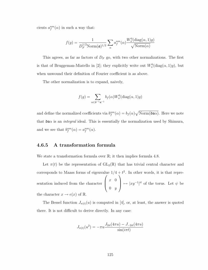
cients anmf (α) in such a way that:
f(g) =1
D1/2F Norm(a)1/2
∑α
anmf (α)W 0π (diag(α, 1)g)√
Norm(α)
This agrees, as far as factors of DF go, with two other normalizations. The first
is that of Bruggeman-Miatello in [2]; they explicitly write out W 0π (diag(α, 1)g), but
when unwound their definition of Fourier coefficient is as above.
The other normalization is to expand, naively,
f(g) =∑
α∈d−1a−1
bf (α)W 0π (diag(α, 1)g)
and define the normalized coefficients via bnmf (α) = bf (α)√
Norm(daα). Here we note
that daα is an integral ideal. This is essentially the normalization used by Shimura,
and we see that bnmf (α) = anmf (α).
4.6.5 A transformation formula
We state a transformation formula over R; it then implies formula 4.8.
Let π(t) be the representation of GL2(R) that has trivial central character and
corresponds to Maass forms of eigenvalue 1/4 + t2. In other words, it is that repre-
sentation induced from the character
x 0
0 y
7→ |xy−1|it of the torus. Let ψ be
the character x→ e(x) of R.
The Bessel function Jπ(t)(u) is computed in [4], or, at least, the answer is quoted
there. It is not difficult to derive directly. In any case:
Jπ(t)(u2) = −πuJ2it(4πu)− J−2it(4πu)
sin(iπt)
125

Let ϕ be a compactly supported function on (0,∞). If we define hϕ(t) by:
hϕ(t) ≡1
2π
∫u∈R
ϕ(u)1
uJπ(t)(u
2)d×u =
∫u
B2it(4πu)ϕ(u)u−1du
where Bν(x) = (2 sin(πν/2))−1(J−ν(x)− Jν(x)), then one checks that:
hϕ(k) =1
2∆(2 cosh(πk))
where hϕ(k) =∫th(t)e2πiktdt and ∆(k) =
∫xϕ(|x|)x−1e2πikxdx. This may be deduced,
for instance, from the results in the Appendix, Subsection 6.3.1. This, accounting for
the appropriate normalization factors, implies Equation 4.8.
126

Chapter 5
Automorphic forms of Galois type
5.1 Introduction
Of course, one would like to extend the work of the previous chapters to cover classi-
fication of π such that L(s, Symrπ) has a pole, for some r ≥ 3. One expects, if such
a form is non-dihedral, that it corresponds to a Galois representation. For example,
if π corresponds to an icosahedral Galois representation with image in SL2(C), then
L(s, Sym12π) has a pole.
We shall briefly discuss in this chapter the reason that the techniques of this thesis
fail to classify such forms in the strong sense that one is able to treat the dihedral
case. This was already pointed out by Sarnak in his letter to Langlands, and analyzed
in sufficient detail to compute the exact bounds needed on the exponential sums in
order to make an improvement. In view of this, we will keep our discussion to a brief
summary of the main obstacle.
We will then relax our aim somewhat: rather than obtaining a spectral formula
that will precisely classify the forms, we use the same technique to bound the number
of these “Galois type” automorphic forms.
As pointed out by Sarnak, it is essentially this idea that underlies the paper of
127

Duke [5] in which he bounds the dimension of weight 1 holomorphic forms for Γ0(q).
(The trivial bound is that the dimension of this space is o(q); Duke improved it to
O(q11/12+ε), and we will improve it further to O(q6/7+ε). This improvement – by
what is essentially exactly the same technique – was simultaneously obtained by P.
Michel. I would like to thank him for interesting discussions on this work and possible
extensions. We have jointly published this, over Q, in [15].)
The precise result is contained in Theorem 6; it is a result that holds over a number
field and over Q gives the result mentioned. It is also possible with some more care
to achieve uniformity in the number field; this will save, I believe, a power of the
discriminant. This extension has not been treated here (nor have I worked it out in
detail, so the suggested conclusion should be regarded with a little caution.)
5.2 Higher Symmetric Powers
As remarked earlier, this material is contained in Sarnak, [17]. We shall sketch how
one can set up a spectral sum that would isolate π for which a higher symmetric
power has a pole, and the obstacle encountered in carrying through the procedure of
the previous chapters.
Let π be an automorphic representation of GL2(AQ); for simplicity we shall assume
that π is unramified at all finite places. At each prime p, let Ap be the Hecke matrix,
so tr(Ap) is the pth coefficient in the L-series of π. To make matters even simpler,
we shall assume the Ramanujan conjecture for all such forms (that is, for all p, Ap
is conjugate to a unitary matrix). The computation that we are about to do makes
sense without this assumption, but its interpretation is a little clearer with it. We
denote by λπ(n) the nth coefficient in the L-series attached to π.
128

The finite part of the symmetric rth power L-function is given by:
L(s, Symrπ) =∏p
det(1− Symr(Ap)p−s)−1
Now, for each p, det(1 − Symr(Ap)p−s)−1 =
∑t≥0 tr(Symt(SymrAp))p
−st = 1 +
λπ(pr)p−s + O(p−2s) where, on account of the Ramanujan conjecture that we are
assuming, the implicit constant in the O is independent of p. In particular, we may
write
det(1− SymrApp−s)−1 = (
∑t≥0
λπ(prt)p−ts)(1 +O(p−2s))
where the implicit constant is still independent of p. Consequently – and possibly
removing Euler factors associated to small prime factors so that the O(p−2s) cause
no problems –
L(s, Symrπ) = E(s)∑n
λπ(nr)n−s
where E(s) is a function with analytic continuation to <(s) > 1/2, and E(1) 6= 0.
In particular, the existence of a pole for L(s, Symrπ) can be analyzed in terms of the
limit:
limX→∞
1
X
∑n<X
λπ(nr)
which is nonzero if and only if the L-function has a pole. The analogue of our earlier
analysis, then, is to carry out the spectral sum:
∑f
1
X
∑n<X
anr(f)am(f)h(tf )
where the sum is over, say, an orthonormal basis of Maass forms for SL2(Z). This
is done, again, via the Kuznetsov formula. Take, for example, the case m = 1. The
geometric side of the formula will then look like (the sum of Chapter 1 now generalized
129

to r 6= 2):
∞∑c=1
∑n<X
S(nr, 1, c)ϕ(4πnr/2
c)
The Kloosterman sum S(nr, 1, c) is dependent only on the residue class of n mod
c. The technique used in Chapter 2 was to break the n-sum into residue classes mod
c. Since ϕ is compactly supported on (0,∞), the n-sum has length around c2/r.
If r = 2, the n-sum has length c, and therefore one expects the n sum to include all
c residue classes; it is therefore reasonable to expect that the exponential sums that
occur are complete – summed over complete residue classes mod c. These exponential
sums are just the S(ν; c, α) that were analyzed in Chapters 2 and 4.
If r > 2, however, the n sum becomes much shorter: even if r = 3, the sum over
n is only of length about c2/3. The exponential sums that occur are therefore funda-
mentally incomplete and their analysis becomes progressively harder as r increases.
Even the gap between r = 2 and r = 3 is enormous.
Therefore, an exact treatment of higher symmetric powers in this fashion is ex-
pected to be a rather difficult endeavor. The goal of the rest of this chapter is to show
how one obtains interesting, though approximate, results, by relaxing our require-
ments: rather than trying to exactly characterize those f such that m(f, Sym12) = 1,
we merely try to bound the number of such f .
This is interesting for other reasons: such forms are associated to Galois represen-
tations, and one can deduce interesting arithmetic information from analytic bounds;
see [5] and [18].
Remark 15. In what follows, it is more convenient, rather than spectrally averaging
the sum ∑n<X
anr(f)
to spectrally average a somewhat more convoluted sum involving sums over various
130
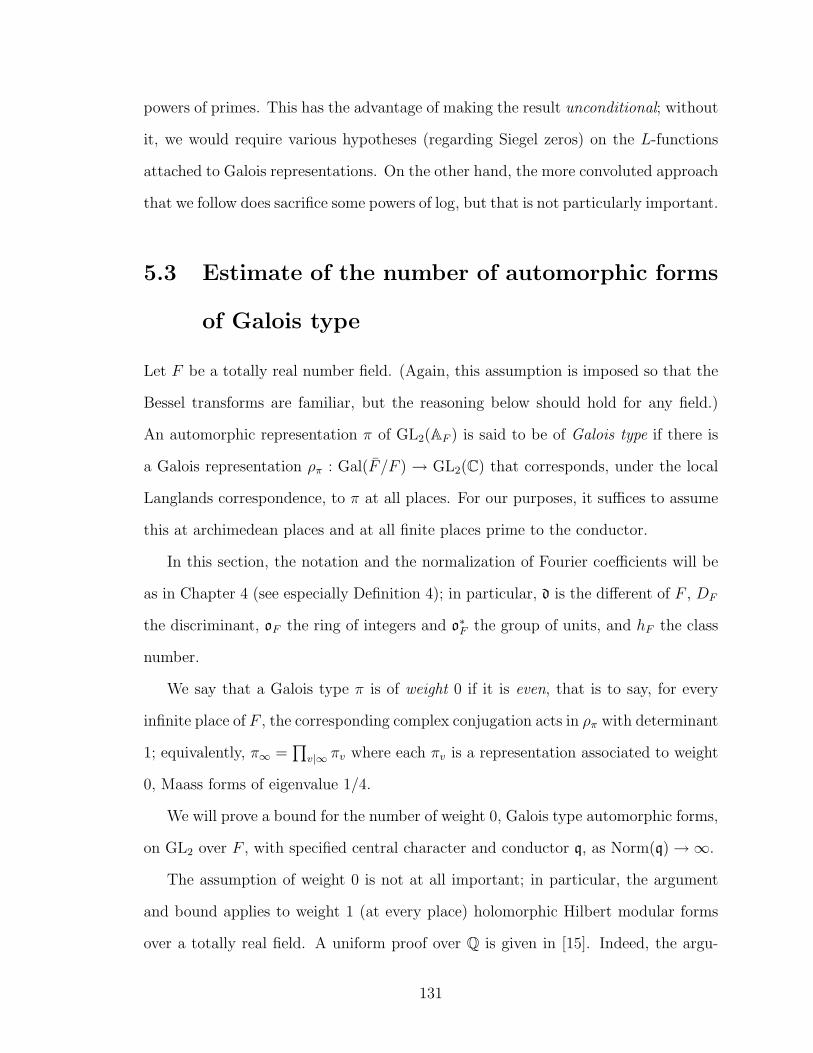
powers of primes. This has the advantage of making the result unconditional; without
it, we would require various hypotheses (regarding Siegel zeros) on the L-functions
attached to Galois representations. On the other hand, the more convoluted approach
that we follow does sacrifice some powers of log, but that is not particularly important.
5.3 Estimate of the number of automorphic forms
of Galois type
Let F be a totally real number field. (Again, this assumption is imposed so that the
Bessel transforms are familiar, but the reasoning below should hold for any field.)
An automorphic representation π of GL2(AF ) is said to be of Galois type if there is
a Galois representation ρπ : Gal(F /F ) → GL2(C) that corresponds, under the local
Langlands correspondence, to π at all places. For our purposes, it suffices to assume
this at archimedean places and at all finite places prime to the conductor.
In this section, the notation and the normalization of Fourier coefficients will be
as in Chapter 4 (see especially Definition 4); in particular, d is the different of F , DF
the discriminant, oF the ring of integers and o∗F the group of units, and hF the class
number.
We say that a Galois type π is of weight 0 if it is even, that is to say, for every
infinite place of F , the corresponding complex conjugation acts in ρπ with determinant
1; equivalently, π∞ =∏
v|∞ πv where each πv is a representation associated to weight
0, Maass forms of eigenvalue 1/4.
We will prove a bound for the number of weight 0, Galois type automorphic forms,
on GL2 over F , with specified central character and conductor q, as Norm(q) →∞.
The assumption of weight 0 is not at all important; in particular, the argument
and bound applies to weight 1 (at every place) holomorphic Hilbert modular forms
over a totally real field. A uniform proof over Q is given in [15]. Indeed, the argu-
131

ment is essentially that of [15] generalized, and also shares many features with [5].
Consequently, we will only sketch certain points that are treated there in more detail;
in each case, the relevant argument generalizes from Q to F .
Theorem 6. Let q be a prime ideal of oF (primality is not essential). Let χ be a
Grossencharacter of conductor dividing q, and let Nχ(q) be the number of automorphic
forms on GL2 over F of Galois type, of weight 0, and with central character χ.
One then has the bound, for any ε > 0,
Nχ(q) F,ε Norm(q)6/7+ε (5.1)
Over Q, this Theorem was proved by Duke, with a weaker exponent (11/12 instead
of 6/7). It is also helpful to keep in mind that the “trivial bound” is Nχ(q)
Norm(q); indeed, the trivial bound is determined by the volume of the symmetric
space, and the index ofK0(q) inK0(oF ) – notation of Subsection 4.2.1 – is Norm(q)+1.
One knows, by a theorem of Deligne-Serre, that all holomorphic forms of weight
1 (over Q) are of Galois type; a similar result holds over totally real fields. It follows
that Theorem 6 gives a bound on the number of automorphic forms of a specified
infinity type, e.g. Theorem 2.
We need to use a slightly sharper form of the Kuznetsov formula than that used in
Chapter 4; this sharper form will allow more versatility in the spectral test function.
(Previously, we were carrying through a limit while fixing the level. If varying the
level, one needs finer control.) This sharper form of the Kuznetsov formula may be
found in Bruggeman-Miatello [2], and the Weil-type bounds for Kloosterman sums
that we will use may be found in [1]. One must modify the formula for the influence
of multiple ideal classes, but this is not difficult. Let χ, q be as in the statement
of Theorem 6. Let χf , χ∞ be defined as in Chapter 4; they are, respectively, the
characters of the finite ideles and of F×∞ obtained by restriction from χ.
132

Let B be an L2-basis for the discrete Laplacian spectrum on
L2χ(GL2(F )\GL2(AF )/F×
∞K0(q)∏v|∞
SO2(Fv))
That is, the space of L2discrete-automorphic forms on GL2(F )\GL2(AF ) that transform
under K0(q) by χf (as in Chapter 4), and are fixed by∏
v|∞ SO2(Fv) and the center
Z(F∞). Note that χ∞ is trivial on account of the weight zero assumption, whence
the assumption on the action of the center Z(F∞).) In particular, this space includes
the Galois type forms of weight 0 with central character χ.
The Kuznetsov formula we will use will be a sum over the set B, which amounts
to considering only “Hilbert Maass forms of weight 0.” As in Chapter 4, Subsection
4.2.1, this set really includes all forms whose central character is an unramified twist
of χ.
Recall from Chapter 4 that we fixed A, a set of representatives for ideal classes
of F . For each a ∈ A and f ∈ B, one has an associated set of Fourier coefficients
af (a, α) for α ∈ a−1d−1. With this notation
Proposition 16. (Kuznetsov formula, after Bruggeman-Miatello) Let a1, a2 ∈ A and
αi ∈ d−1a−1i . Then:
∑f∈B
af (a1, α1)af (a2, α2)hf (ϕ) + Continuous Spectrum Contribution = δa1,a2·
h0(ϕ)δ′α1,α2D
1/2F +
∑c∈qa−1
1 −0
∑ε∈o∗F /(o
∗F )2
1
Norm(ca1)KSχ(α, εα
′; c)ϕ(αα′ε
c2)
where δ′(α1, α2) = 1 if α1α
−12 is a unit, and 0 otherwise. ϕ is a function on F ⊗
R = Rd that is a product of functions at each place. ϕ is assumed to be supported
on F∞,+ = (R+)d, the multiquadrant of totally positive elements. f 7→ hf (ϕ) is
a spectral transform of ϕ. The Kloosterman sum is defined as KSχ(A,B;C) =
133

∑x∈(oF /a1C)× χf (x)e(tr(
Ax+Bx−1
C)); it strictly depends on a1, but we suppress that de-
pendence.
Remark 16. The phrasing of this formula is a little different to that of Chapter 4;
namely, we have replaced o∗,+F /(o∗F )2 with o∗F/(o∗F )2, and have replaced ϕ(x) by ϕ(x2).
There is no change in the underlying substance; this new phrasing just allows us to
avoid the “total positivity” Remark 10 of Chapter 4, which would be a little annoying
to have to deal with in what follows. Of course, this changes the transformation rule
ϕ 7→ hf (ϕ), but we will have no need for the explicit formula, using only Lemma 19
below.
Lemma 19. We may choose ϕ so that the spectral transform satisfies hf (ϕ) > 0 for
all f , and ϕ satisfies the following decay estimates:
ϕ(x) k
∏v
min(xkv , 1), forx = (xv) ∈ F∞ =∏v|∞
Fv (5.2)
this holding for all k.
Proof. This is well-known over Q – see for example the explicit functions in [15]; the
result follows over F by taking ϕ to be a product of the Q-test functions.
As far as I know, one cannot achieve this positivity for the larger spectral sum
used in Chapter 4 – the restriction to a particular weight (weight 0 in our case) is
essential.
In our normalization, the average size of the coefficients af (a, α) is approximately
(hFDFNorm(q))−1/2. Let λf (m) denote the mth Hecke eigenvalue of f , for m an
integral ideal of F . As in Chapter 4, the coefficients λf are related to af via af (a, α) =
Cfλf (aαd), where |Cf |2 is essentially the reciprocal of a special value of an L-function.
Lemma 20. If f satisfies the Ramanujan-Petersson conjecture – in particular, if f is
associated to a Galois representation – then the constant Cf F,ε Norm(q)−1/2−ε.
134

Proof. This is proved as in [5]. The idea is as follows: |Cf |2 is the reciprocal of a
special value of an L-function at 1. This L-function can be estimated with a very
short partial sum; the assumption on Ramanujan-Petersson gives a bound on the
coefficients that occur, whence an upper bound for the L-function and a lower bound
on Cf . Indeed, one can establish the required bound on the L-function without using
the fact that f is of Galois type, by using an argument of Iwaniec; the bound is then
very slightly weaker (only by Norm(q)ε).
The L-series of f is given in terms of the λf via L(s, f) =∑
Iλf (I)
Norm(I)s , when the
sum is extended over integral ideals I of F .
5.3.1 Existence of an amplifier
As in Duke [5] or Wong [18], one can construct an “amplifier” that picks out forms
of Galois type. (Recall Remark 15.)
For example, suppose f is a form with central character χ that is associated to
an icosahedral Galois representation. (The composition of the Galois representation
with determinant is then the character of Gal(F/F ) associated, by class field theory,
to χ.)
Fix an integer N , which will be optimized at the end of the argument. Following
Duke and Wong, we define a sequence aIcoI (an “amplifier” for icosahedral forms),
indexed by integral ideals I of F and so that, if p denotes a prime ideal of F ,
aIcoI =
χ(p)6, for I = p12,Norm(p) ≤ N1/12, (p, q) = 1
−χ(p)4, for I = p8,Norm(p) ≤ N1/12, (p, q) = 1
−χ(p), for I = p2,Norm(p) ≤ N1/12, (p, q) = 1
0 else.
135

The point of this is that, for any prime ideal p prime to q, we have the equality
−χ(p)λf (p2)− χ(p)4λf (p
8) + χ(p)6λf (p12) = 1
This is a consequence of f being associated to an icosahedral Galois representation.
(See [18]).
For convenience, we set T to be the number of prime ideals of norm less than
N1/12; thus T ε N1/12−ε.
In particular, the sum
∑I
aIcoI λf (I)
∑Norm(p)<N1/12
p prime
1 = T (5.3)
Proof. (of Theorem) We form the spectral sum, with hf and ϕ chosen, and fixed as q
varies, according to Lemma 19,
S =∑f∈B
hf (ϕ)|Cf |2|∑
I
aIcoI λf (I)|2 + Continuous Spectrum Contribution
where the continuous spectrum contribution is defined analogously, and we suppress
it; the only needed fact is that it is positive. See also [15] for a precise expression
over Q.
By Lemma 20 and Equation 5.3, we see that:
S Nχ(q)T2Norm(q)−1−ε (5.4)
Now, we split up the sum S into hF sub-sums depending on the ideal class of I.
Recall A is a set of representatives for the ideal classes of F . Each sub-sum involves
about h−1F T ideals. (We are not aiming for uniformity in F , so factors of h−1
F will
eventually be neglected.) As in Chapter 4, it becomes expedient to introduce a “twist’
136

by the different in considering the ideal class representatives; we do this in Equation
5.5 below.
S =∑
f
hf (ϕ)|∑a∈A
∑I∼ad
aIcoI Cfλf (I)|2 + Continuous Spectrum Contribution (5.5)
We expand the inner sum and use the Kuznetsov formula Proposition 16, together
with the comments preceding Lemma 20.
S =∑
a
∑r∈a−1d−1/o∗Fs∈a−1d−1/o∗F
aIco(r)ada
Ico(s)ad
h0D1/2F δ′r,s +
∑ε∈o∗F /(o
∗F )2
∑c∈a−1q
KSχ(r, s; c)
Norm(ca)ϕ(rsε
c2)
(5.6)
Here a−1d−1/o∗F means elements of a−1d−1 modulo multiplication by units, and
(r), (s) denote the ideals generated by r and s.
Each internal sum in Equation 5.6 is over about h−1F T values of r and s. That
is, given a there are about h−1F T classes [r] ∈ a−1d−1/o∗F for which aIco
(r)ad 6= 0. Since
we are not looking for uniformity in F , we will simply use the bound that there are
O(T ) values of r, s.
As far as the coefficients aIcoI go, we apply only the trivial estimate |aIco
I | 1.
For fixed a, in view of the rapid decay of ϕ near 0, the c sum extends over all c
with Norm(c)2 Norm(rs)1+ε. Since the coefficients aIco(r)ad are nonzero only for
Norm((r)ad) N , we see that Norm(r) NNorm(a)−1D−1F , and so the sum includes
only c with:
Norm(ca) (ND−1F )1+ε F N
1+ε (5.7)
Put c = (c)a – it is an ideal contained in q. We shall use the “Weil estimate”: if
c ∈ a−1, r, s ∈ a−1d−1 and c = (c)a, then
KSχ(r, s; c) F Norm((rad, sad, c))1/2Norm(c)1/2+ε
137

Here (B1,B2,B3) means the greatest common factor of the ideals Bi. The derivation
of this is similar to that over Q: appeal to an algebro-geometric estimate at primes;
one can use a direct estimate (“stationary phase”!) at prime powers, and use multi-
plicativity to piece them together. Without the character χ, this bound is contained
in [1]. The Norm((rad, sad, c))1/2 factor is entirely harmless, since “very few” r, s
have a common factor with c. (To formally justify this, split the sum in Equation 5.6
up into classes according to the value of Norm((rad, sad, c))1/2.)
We wish to sum over the ideals c rather than the elements c. In order to do this,
we need to bound the sum over all c corresponding to a given c, that is, fixing c0 we
wish to sum over all all c = c0ε′ with ε′ ∈ o∗F . To do this, we utilize Lemma 15 of
Chapter 4 and we use the rapid decay (expressed in Lemma 19) of ϕ. We obtain, for
any k > 0 and any δ > 0,
|∑c=c0ε′
ϕ(rsc−2)| k,δ min(Norm(rs/c2)δ,Norm(rs/c2)k−δ)
Considerations such as those leading to Equation 5.7 show that this amounts to say
that the ϕ-sum associated to each c contributes, in total, at most N ε and the sum of
Equation 5.6 is essentially restricted to Norm(c) N1+ε.
Finally, in Equation 5.6, the sum over o∗F/(o∗F )2 is over a finite set and only
contributes an additional constant.
Combining all the previously-mentioned estimates, we obtain for all ε > 0:
S F,ε Nε
T + T 2∑
q|c,Norm(c)N1+ε
Norm(c)−1/2+ε
and therefore
S F,ε
(T + T 2Norm(q)ε
N1/2
Norm(q)
)N ε
138

Combining this estimate with Equation 5.4, we find:
Nχ(q) F,ε
(Norm(q)1+εT−1 + Norm(q)εN1/2
)N ε
The optimal value for N is N = Norm(q)12/7, which gives T = Norm(q)1/7−ε. This
verifies the bound of Theorem 6 for f that are associated to icosahedral Galois rep-
resentations. Similarly, one obtains bounds for dihedral, octahedral and tetrahedral
which are strictly better (because the corresponding sequences aDihedral, aOct, aTetra
are less sparse; this is closely related to the fact that one does not need to go to the
twelfth symmetric power to find a pole.)
Therefore, Theorem 6 holds for all Galois-type forms together.
139

Chapter 6
Appendix
6.1 Classification of Dihedral Forms
We discuss here what is expected, from general theory, about the classification of
“dihedral” forms over a number field. Let F be a number field and LF the conjec-
tural “Langlands group” whose complex representations parameterize automorphic
representations. We are only interested in heuristics here, and so the fact that this
conjectural is not problematic.
Let π be an automorphic, cuspidal representation of GL2(AF ); suppose it is pa-
rameterized by a map ρπ : LF → GL2(C).
Suppose the symmetric-square L-function of π has a pole. Then, one expects the
representation ρπ parameterizing π to factor through the orthogonal group O(2,C);
in particular, by composition with determinant, we find a map LF → ±1. This
map should factor through the Galois group Gal(F/F ); in particular, it determines
a quadratic extension K, and a map LK → SO(2,C) = Gm(C).
One then expects that there is a quadratic extension K of F , and a GL(1) form ω
(i.e. a Grossencharacter) of K with the property that ωσ = ω−1, where σ is the Galois
automorphism of K over F , so that the L-function of π and L(s, ω,K) agree. The
140
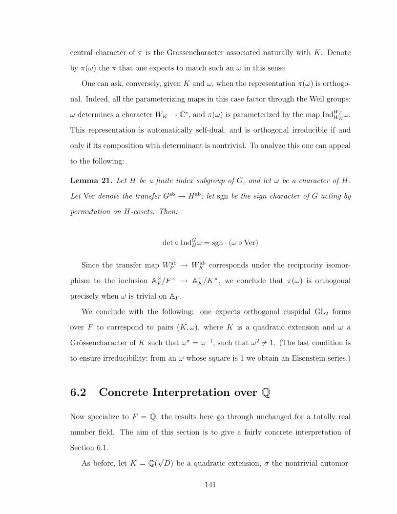
central character of π is the Grossencharacter associated naturally with K. Denote
by π(ω) the π that one expects to match such an ω in this sense.
One can ask, conversely, given K and ω, when the representation π(ω) is orthogo-
nal. Indeed, all the parameterizing maps in this case factor through the Weil groups:
ω determines a character WK → C∗, and π(ω) is parameterized by the map IndWFWK
ω.
This representation is automatically self-dual, and is orthogonal irreducible if and
only if its composition with determinant is nontrivial. To analyze this one can appeal
to the following:
Lemma 21. Let H be a finite index subgroup of G, and let ω be a character of H.
Let Ver denote the transfer Gab → Hab; let sgn be the sign character of G acting by
permutation on H-cosets. Then:
det IndGHω = sgn · (ω Ver)
Since the transfer map W abF → W ab
K corresponds under the reciprocity isomor-
phism to the inclusion A×F/F
× → A×K/K
×, we conclude that π(ω) is orthogonal
precisely when ω is trivial on AF .
We conclude with the following: one expects orthogonal cuspidal GL2 forms
over F to correspond to pairs (K,ω), where K is a quadratic extension and ω a
Grossencharacter of K such that ωσ = ω−1, such that ω2 6= 1. (The last condition is
to ensure irreducibility; from an ω whose square is 1 we obtain an Eisenstein series.)
6.2 Concrete Interpretation over Q
Now specialize to F = Q; the results here go through unchanged for a totally real
number field. The aim of this section is to give a fairly concrete interpretation of
Section 6.1.
As before, let K = Q(√D) be a quadratic extension, σ the nontrivial automor-
141

phism of K, and K∞ = K⊗R. D is chosen to be a fundamental discriminant, so |D|
is the discriminant of K over Q.
Characters of prescribed conductor
We start by explicitly describing the characters ω of A×K/A
×QK
× such that π(ω) has
prescribed conductor.
Note that triviality of ω on A×Q implies ωσ = ω−1. The most convenient phrasing
will be in terms of orders of K. We state most of the relevant facts without proof.
Definition 11. For each finite place v of K, let ov be the maximal compact subring
of Kv and pv the maximal ideal. The local conductor of ω at v is defined as fv = pmv ,
where m is the least non-negative integer such that ω is trivial on 1 + pmv . The global
conductor of ω is defined as fω =∏
v finite fv.
The conductor of the GL(2) automorphic form π(ω) is then given by
N = |D|Norm(fω)
since |D| is the discriminant of K. To distinguish the two, we shall refer to fω as the
K-conductor of ω.
Lemma 22. Suppose ω is a character of A×K/K
× that is trivial on A×Q. Then the
K-conductor fω = (f) for some f ∈ Z, i.e. it is the extension of an ideal of Q, and
the corresponding π(ω) has conductor |D|f 2.
Lemma 23. Let f ∈ Z. For v a finite place of K, above the prime p of Q, let Uv(f)
be the open subgroup of K×v given by (1 + fov)Z×
p .
Let U(f) =∏
v Uv(f) =∏
v(1 + fov) ·∏
p Z×p . A character ω, trivial on AQ, has
K-conductor dividing (f) if and only if it is trivial on U(f).
142

Characters for which π(ω) has conductor dividing N = |D|f 2, and equivalently ω
has K-conductor dividing (f), are thus just the characters of
C(f) = A×K/(A
×QK
×U(f)) = A×K/R
×K×U(f)
We are interested, then, in understanding C(f). (We include the tilde to remind the
reader that C(f) is much larger than the class group, since it includes an archimedean
torus.)
Let Λ be the group of units of oK , the ring of integers in K. Let Λ(f) be the
group of units of K that lie in U(f) at finite places. Then C(f) fits into an exact
sequence:
K×∞/R×Λ(f) C(f) A×
K/(K×∞K
×U(f)) (6.1)
The final group CD,f = A×K/(K
×∞K
×U(f)) fits into an exact sequence:
Λ/Λ(f) → U(1)/U(f) → CD,f → A×K/(K
×∞U(1))
Note that the final group is just the class group, with cardinality the class number
hD. The cardinality of CD,f therefore equals:
hDf∏p|f
(1− χ(p)/p)/[Λ : Λ(f)]
where the product is over primes p dividing f . We shall denote this number by hD,f .
It is, in fact, the class number of the quadratic order with discriminant Df 2.
On the other hand, we can easily describe the initial group of Equation 6.1:
K×∞/R×Λ(f). If K is a real field, K∞ = R ⊕ R and this quotient is isomorphic
to R×/Λ(f), where Λ(f) is embedded in R× via either of the embeddings of K into
R. If Λ(f) contains an element of norm −1, this group is a connected torus (indeed
an S1); otherwise, it is disconnected. If K is a complex field, i.e. K∞ = C, then
143

K×∞/R×Λ(f) is always a connected torus.
Orders
Let oD,f be the (unique) order of discriminant Df 2; the groups mentioned above will
be easily interpretable in terms of oD,f . By definition, oD,f = Z + foD, a subring of
Q(√D). Uv(f) is the unit group in the closure (oD,f )v of oD,f in Kv, and as before
U(f) =∏
v Uv(f). Λ(f) is the group of units of oD,f . The group CD,f is the class
group of oD,f , and hD,f its class number.
6.2.1 Fourier Coefficients
Let λm(ω) be the m-th coefficient of the L-series of π(ω). Suppose m is coprime to
Df 2. Let (m) be the ideal generated by m. Then
λm(ω) =∑
N(I)=(m)
ω(I) (6.2)
where I ranges over ideals and we regard ω as a character of ideals in the natural
way.
Now let us sum λm(ω) over all ω of K-conductor dividing (f) with a prescribed
infinity component ω∞, i.e. restriction to K×∞ = (K ⊗ R)×. As we have seen, the
set of such is a principal homogeneous space for the group of characters of CD,f =
A×K/K
×∞K
×U(f). When we sum λm(ω) over such ω, the sum over ideals I in Equation
6.2 is cut down to a sum over principal ideals I that are generated by an element of
oD,f . Let X±m be a set of representatives for elements x ∈ oD,f such that Norm(x) =
±m, modulo units of oD,f . ω∞ is a character of K∞ trivial on Λ(f) and so, for
x ∈ Xm, to evaluate ω∞(x) makes sense.
144

We obtain: ∑ω,ω∞ fixed
λm(ω) = hD,f∑
x∈X±m
ω∞(x) (6.3)
Now, if K is a real field and Λ(f) contains no element of norm −1, then characters
ω∞ come in pairs: ω∞ and ω′∞ are paired when their restriction to the connected
component ofK×∞ are identical. Denote by ω∞,+ the restriction of ω∞ to the connected
component of K×∞.
For m < 0, in this setting, define λm(ω) = ±λ|m|(ω) according to whether the
Maass form π(ω) is even (positive sign) or odd (negative sign). (That may be com-
puted from ω∞ as follows: R× sits inside K×∞ as elements of norm one; π(ω) is even
or odd depending on whether ω∞ restricted to this R× factors through absolute value
or not.)
One then deduces, where Xm is a set of representatives for x ∈ oD,f of norm m,
modulo units in oD,f of norm 1:
∑ω,ω∞,+fixed
λm(ω) = 2hD,f∑x∈Xm
ω∞,+(x) (6.4)
6.2.2 Summary of Results
If ω, a Grossencharacter of K, has K-conductor (f), the representation π(ω) has
conductor |D|f 2. As ω ranges over all Grossencharacters of K, trivial on AQ, of
conductor dividing (f), π(ω) ranges over all representations with central character
χD and with conductor dividing |D|f 2, whose symmetric square has a pole. It is
exactly these forms which will be found on Γ0(|D|f 2). Finally, ω∞ will determine the
real type of π(ω) as follows: if K is real and ω∞ is the character of R× × R× taking
(x, x−1) 7→ sgn(x)εω |x|itω , then π(ω) corresponds to a Maass form of eigenvalue 1/4+t2ω
and parity εω; if K is complex and ω∞ is the character z 7→ zkω−1z−kω+1 of C×, then
π(ω) is holomorphic of weight kω.
145

Real Quadratic Case: First suppose K is real quadratic. Let ε0 be a fundamental
unit for oD,f : a generator for Λ(f). There are two cases:
1. Norm(ε0) = −1. In this case, the tω are the integral multiples of iπ/2 log(ε0),
and so one expects to find Maass forms for (Γ0(Df2), χD) of eigenvalue 1/4−r2,
with r = iπn2 log(ε0)
and n ∈ Z. If n is even the Maass forms are even and if n is
odd the Maass forms are odd. Each n occurs with multiplicity hD,f . The sum
of Fourier coefficients is given by Equation 6.3.
2. Norm(ε) = 1. In this case, the tχ are the integral multiples of iπ/ log(ε0), and
so one expects to find Maass forms for (Γ0(Df2), χD) of eigenvalue 1/4 − r2,
with r = iπnlog(ε0)
and n ∈ Z. Each n occurs with multiplicity 2hD,f , and half the
forms are odd, half even. The sum of Fourier coefficients is given by Equation
6.4.
Holomorphic Case: Now suppose that ω is a character of an imaginary quadratic
field. Let |Λ(f)| = wf ; it is the number of roots of unity in the order oD,f . The possible
infinity types of π(ω) are just those discrete series of weight k, with k congruent to 1
mod wf (in particular, always odd). The multiplicity of each kω is again hD,f . In this
case, m is always positive and the sum of Fourier coefficients is given by Equation
6.3.
6.3 Bessel Transforms and Inversion Questions
6.3.1 Fourier transforms and Bessel Transforms
Let ϕ(x) be a function, which has reasonable decay near 0 and infinity. Here we prove
some identities relating ϕ and its Bessel transform.
Define
h+(t) =
∫ ∞
0
B2it(x)ϕ(x)x−1dx
146
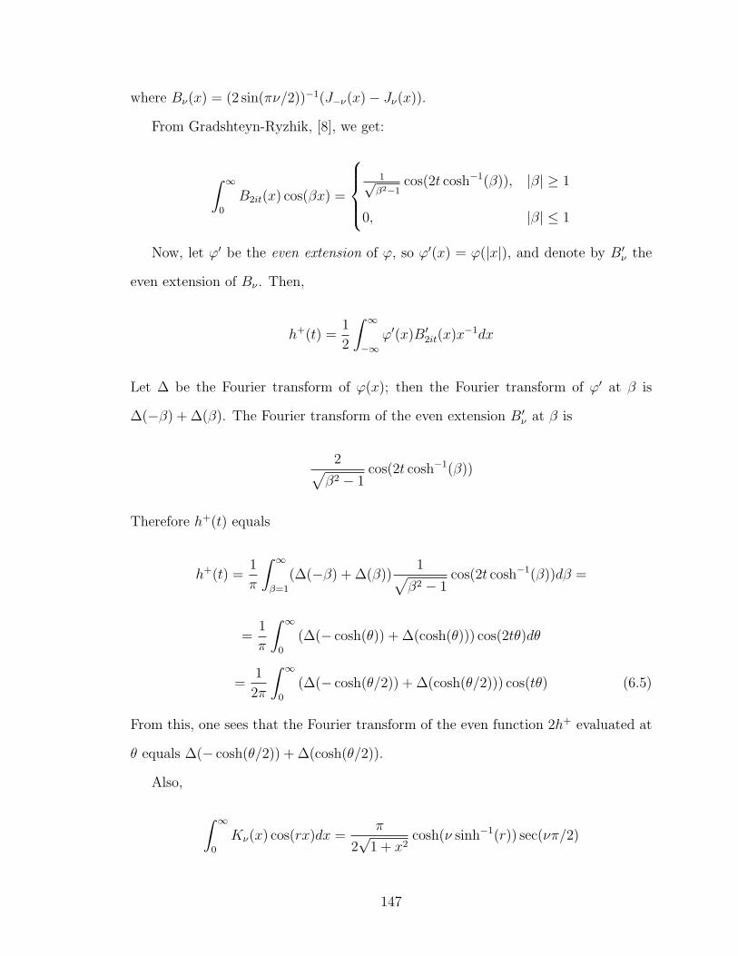
where Bν(x) = (2 sin(πν/2))−1(J−ν(x)− Jν(x)).
From Gradshteyn-Ryzhik, [8], we get:
∫ ∞
0
B2it(x) cos(βx) =
1√β2−1
cos(2t cosh−1(β)), |β| ≥ 1
0, |β| ≤ 1
Now, let ϕ′ be the even extension of ϕ, so ϕ′(x) = ϕ(|x|), and denote by B′ν the
even extension of Bν . Then,
h+(t) =1
2
∫ ∞
−∞ϕ′(x)B′
2it(x)x−1dx
Let ∆ be the Fourier transform of ϕ(x); then the Fourier transform of ϕ′ at β is
∆(−β) + ∆(β). The Fourier transform of the even extension B′ν at β is
2√β2 − 1
cos(2t cosh−1(β))
Therefore h+(t) equals
h+(t) =1
π
∫ ∞
β=1
(∆(−β) + ∆(β))1√β2 − 1
cos(2t cosh−1(β))dβ =
=1
π
∫ ∞
0
(∆(− cosh(θ)) + ∆(cosh(θ))) cos(2tθ)dθ
=1
2π
∫ ∞
0
(∆(− cosh(θ/2)) + ∆(cosh(θ/2))) cos(tθ) (6.5)
From this, one sees that the Fourier transform of the even function 2h+ evaluated at
θ equals ∆(− cosh(θ/2)) + ∆(cosh(θ/2)).
Also,
∫ ∞
0
Kν(x) cos(rx)dx =π
2√
1 + x2cosh(ν sinh−1(r)) sec(νπ/2)
147

so, in particular, from the definition
h−(t) =4
πcosh(πt)
∫ ∞
0
K2it(x)ϕ(x)x−1dx
we obtain
h−(t) =1
π
∫ ∞
0
1√1 + β2
(∆(β) + ∆(−β)) cos(2t sinh−1(β))dβ
which gives, just as before:
h−(t) =1
2π
∫ ∞
0
(∆(sinh(θ/2)) + ∆(− sinh(θ)/2) cos(tθ)dθ
and so:
h−(λ) = h−(−λ) =1
2(∆(sinh(λ/2)) + ∆(− sinh(λ/2)))
6.3.2 Inversion problem
The purpose of this section is to verify that one obtains a “large enough” collection
of spectral functions h from geometric functions ϕ with compact support in (0,∞).
We will sketch this in the hardest case (the J-transform); in each case, the key
point is that, as in the Paley-Wiener theorem, allowing spectral transforms to have
holomorphic extensions forces the geometric function to have good decay. The central
result is Theorem 7 below. It also suffices for the implicit application in Chapter 4
by taking a function of the type constructed below at every infinite place. We also
will use implicitly various results on Bessel functions, for which we refer to [8].
Note that one must be careful, in these arguments, to avoid complications that
arise from exceptional eigenvalues. We do not discuss this issue explicitly, and check
our bounds only at those eigenvalues which are non-exceptional, but the arguments
given are valid even in the presence of exceptional eigenvalues, as the reader can
148

check.
We note that the formulas for the Sears-Titchmarsh inversion in the appendix
of Iwaniec appear to be incorrect, although this does not affect the truth of the
Kuznetsov formula presented. Kuznetsov’s original paper, [11], provides a treatment
and derivation of the formula.
The transform of interest is (note that the hϕ,k are only of interest for k an odd
integer):
ϕ→(h+ϕ (t) =
∫B2it(x)ϕ(x)x−1dx, hϕ,k =
∫Jk(x)ϕ(x)x−1
)(6.6)
Here Bν(x) = (2 sin(πν/2))−1(J−ν(x) − Jν(x)). In particular, for ν = k, an odd
integer, Bk(x) = (−1)(k−1)/2J−k(x). Therefore, for ϕ of compact support, (h+ϕ , hϕ,k)
are, up to sign, the values of a holomorphic function h(z) along the imaginary axis
and at odd integers.
This is inverted via the Sears-Titchmarsh inversion formula:
(h+(t), hk) → ϕ(x) = 4
∫ ∞
0
B2it(x)h+(t)t tanh(πt)dt+
∑k≡1(2)
2khkJk(x) (6.7)
(The factor of 4 is missing from Iwaniec.) These transformations can be regarded
as an isometry between appropriate Hilbert spaces, but we will not have need of this.
Theorem 7. Let tj be a discrete subset of R with #j : tj ≤ T T r for some r.
Let, for each j, there be given a function cX(tj) depending on X, so that cX(tj) tr′j
for some r′ – the implicit constant independent of X; similarly, for each k odd, let
there be given a function cX(k) depending on X so that cX(k) kr′.
Suppose that one has an equality
limX→∞
(∑j
cX(tj)h+ϕ (tj) +
∑k odd
cX(k)hϕ,k
)= 0 (6.8)
149
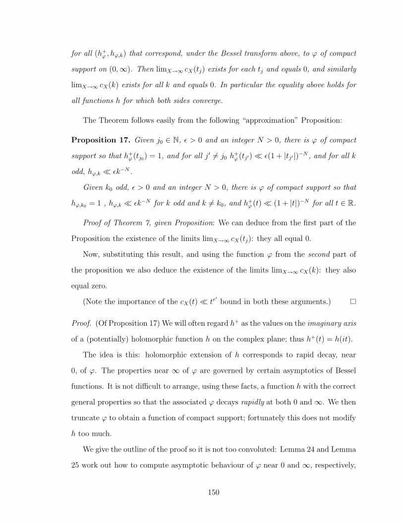
for all (h+ϕ , hϕ,k) that correspond, under the Bessel transform above, to ϕ of compact
support on (0,∞). Then limX→∞ cX(tj) exists for each tj and equals 0, and similarly
limX→∞ cX(k) exists for all k and equals 0. In particular the equality above holds for
all functions h for which both sides converge.
The Theorem follows easily from the following “approximation” Proposition:
Proposition 17. Given j0 ∈ N, ε > 0 and an integer N > 0, there is ϕ of compact
support so that h+ϕ (tj0) = 1, and for all j′ 6= j0 h
+ϕ (tj′) ε(1 + |tj′|)−N , and for all k
odd, hϕ,k εk−N .
Given k0 odd, ε > 0 and an integer N > 0, there is ϕ of compact support so that
hϕ,k0 = 1 , hϕ,k εk−N for k odd and k 6= k0, and h+ϕ (t) (1 + |t|)−N for all t ∈ R.
Proof of Theorem 7, given Proposition: We can deduce from the first part of the
Proposition the existence of the limits limX→∞ cX(tj): they all equal 0.
Now, substituting this result, and using the function ϕ from the second part of
the proposition we also deduce the existence of the limits limX→∞ cX(k): they also
equal zero.
(Note the importance of the cX(t) tr′bound in both these arguments.)
Proof. (Of Proposition 17) We will often regard h+ as the values on the imaginary axis
of a (potentially) holomorphic function h on the complex plane; thus h+(t) = h(it).
The idea is this: holomorphic extension of h corresponds to rapid decay, near
0, of ϕ. The properties near ∞ of ϕ are governed by certain asymptotics of Bessel
functions. It is not difficult to arrange, using these facts, a function h with the correct
general properties so that the associated ϕ decays rapidly at both 0 and ∞. We then
truncate ϕ to obtain a function of compact support; fortunately this does not modify
h too much.
We give the outline of the proof so it is not too convoluted: Lemma 24 and Lemma
25 work out how to compute asymptotic behaviour of ϕ near 0 and ∞, respectively,
150

given h. Once this is done, Lemma 26 shows that one can obtain the first part of
Proposition 17 with a function ϕ which has at least “very good” decay near 0 and ∞,
and Lemma 27 does the same for the second part of Proposition 17. Finally, Lemma 28
and Lemma 29 show that these ϕ can be truncated to have compact support without
affecting the functions h too much, thus establishing Proposition 17 as stated.
Throughout we will be dealing with functions so that both h+(t) and hk decay
very rapidly (faster than any polynomial). Therefore, the convergence of series and
the interchange of various sums and series is easy to justify, and we do not explicitly
comment on this.
First, we address the issue of holomorphic extension of h and the decay near 0
of ϕ. We say a holomorphic function f has rapid decay along vertical lines if, for
fixed σ, f(σ + it) decays faster than any polynomial in t, for t real. We say it has
super-exponential decay if, along the line s = σ + it, f(s) decays faster than any
exponential function in t. For example, f(s) = es2
has super-exponential decay.
Lemma 24. Let A be a positive integer. Suppose there exists a function h(z), holo-
morphic for |<(z)| ≤ A+ ε for some ε > 0, and rapidly decaying along vertical lines,
so that h+(t) = h(it) and hk = (−1)(k−1)/2h(k). Let ϕ = Fh be the function associated
to (h+, hk) by Sears-Titchmarsh inversion. Then one has an estimate for ϕ and its
derivatives near 0, given by ϕ(l)(x) xA−l.
Proof. Write, noting that sin(πit) = i sinh(πt),
ϕ(x) = 2i
∫t≥0
1
cosh(πt)h+(t)tJ2it(x)dt −2i
∫t≥0
1
cosh(πt)h+(t)tJ−2it(x)dt
+∑k≡1(2)
2khkJk(x) (6.9)
= 2i
∫t
1
cosh(πt)h+(t)tJ2it(x)dt+
∑k
· · ·
One now shifts lines of integration from =(t) = 0 to =(t) = A. The residues coming
151

from the integral cancel the contribution of the “discrete sum”∑
k 2khkJk(x), and
one need only appeal to the power series expansion of the Bessel function to deduce
the claimed estimate.
For the derivatives, use the differentiation formulae for Bessel functions.
If h is a holomorphic function as in the previous Lemma, we will always de-
note by Fh the function attached to (h+(t) = h(it), hk = (−1)(k−1)/2h(k)) by Sears-
Titchmarsh inversion.
The key to good decay of ϕ near zero, then, is holomorphic extension. We now
must address the question of obtaining good decay for ϕ near ∞.
Lemma 25. Suppose h+(t) decays super-exponentially, that is to say, h+(t) A e−A|t|
for all A, and similarly for hk. Then the function ϕ associated to (h+, hk) by Sears-
Titchmarsh inversion has the asymptotic expansion:
ϕ(x) = cos(x− π/4)∑n≥1
Anx−n/2 + sin(x− π/4)
∑n≥1
Bnx−n/2
The error at truncating at n is of the order of the next term. Here An is given by a
linear form in (h+, hk):
An(h) = 4
∫ ∞
0
an(2it)h+(t)t tanh(πt)dt+
∑j
2jan(j)hj
where an(z) are certain polynomials in z, and Bn(h) is defined similarly, with corre-
sponding polynomials bn(z). Each derivative ϕ(l)(x) also has an asymptotic expansion,
equal to that obtained by term by term differentiation.
Proof. Indeed, one has an asymptotic for the Bessel functions.
Bν(x) = cos(x− π/4)n∑k=1
ak(ν)x−k/2 + sin(x− π/4)
n∑k=1
bk(ν)x−k/2 +R
152

where the remainder is R = O(e|3πν/2|x−(n+1)/2) and ak(ν), bk(ν) is a polynomial in
ν. The implicit constant is absolute. (Almost certainly one can improve on this
remainder: this is merely what I obtain from analyzing the argument in Whittaker’s
treatise on Bessel functions, and it suffices for the argument here.)
It follows that ϕ(x) = 4∫tB2it(x)h
+(t)t tanh(πt)dt+∑
k hkJk(x) also satisfies an
asymptotic (and this is easy to justify from the explicit estimate of the remainder
term noted above):
ϕ(x) = cos(x− π/4)n∑k=1
Akx−k/2 + sin(x− π/4)
n∑k=1
Bkx−k/2 +O(x−(n+1)/2)
Here
Ak(h) = 4
∫ ∞
0
ak(2it)h+(t)t tanh(πt)dt+
∑j
2jak(j)hj
and Bk(h) is defined similarly. Similar asymptotics hold for the derivatives of ϕ.
(The asymptotics for the derivatives of Bessel functions are easily deduced from the
ones above, since one can express the derivative of a Bessel function in terms of other
Bessel functions. For example, J ′ν(z) = 12(Jν−1(z)− Jν+1(z)).
Lemma 26. Fix an integer M and j0 ∈ N, ε, N . There exists a holomorphic function
h, of super-exponential decay along any vertical line, so that h(k) = 0 for k inte-
gral, and so h+(t) = h(it) satisfies the conditions of the first part of Proposition 11
(i.e. h(itj0) = 1, and for j′ 6= j0 h′(itj′) ε(1 + |tj′|)−N), so that additionally the
asymptotic constants An(h) and Bn(h) from the Lemma 25 vanish for n < 2M . In
particular, Fh(x) = O(x−M).
Proof. We need to check that there is a function h with the desired properties so that
Ak(h) = Bk(h) = 0 for k ≤ 2M . That this should be possible is (loosely speaking)
clear, since one has a finite number of compatible linear constraints on an infinite-
153

dimensional space; however, one must be careful in doing this without jeopardizing
the necessary growth properties. The idea is to pick some basic localized test functions
and then take an appropriate linear combination to satisfy the constraints. We will
only sketch the argument.
Fix a real number T and δ > 0. Define hT,δ(z) = 2Tδ√πe−((z2+T 2)/δ)2 T sin(πz)
(z sin(πT ))– the
construction has to be slightly modified for T = 0, which we leave to the reader.
Then hT,δ is holomorphic and, as δ → 0, localized around t = ±iT – or, to be precise,
h restricted to R ∪ iR is localized there.
It also has zeros for t integral. It has super-exponential decay along vertical lines,
and the property that∫t∈R hT,δ(it) → 1 as δ → 0 (the constants in hT,δ were chosen
so that this is true.)
Fix a finite set of real numbers Tj, for 1 ≤ j ≤ Q. Eventually we shall fix
matters so precisely one of the Tj is a tj. Now write, for some constants cj that are
to be specified, a new function hδ as a linear combination of our basic test functions:
hδ(z) =
Q∑j=1
cjhTj ,δ(z)
for certain Ti. The idea is that by letting δ → 0 and taking the correct linear combi-
nation one can fulfill the linear constraints and the growth conditions simultaneously.
hδ still has zeros at all integral arguments and holomorphic extension to the entire
complex plane. Let Fδ be the function defined by Sears-Titchmarsh inversion starting
from hδ (i.e. starting from h+δ (t) = hδ(it), hk = 0).
Thus, function Fδ has, on account of the holomorphicity of hδ, arbitrarily rapid
polynomial decay near 0. Its decay near ∞ is governed by the coefficients:
Ak(hδ) = 4
Q∑j=1
cj
∫ ∞
−∞hTj ,δ(it)ak(2it)t tanh(πt)dt
154
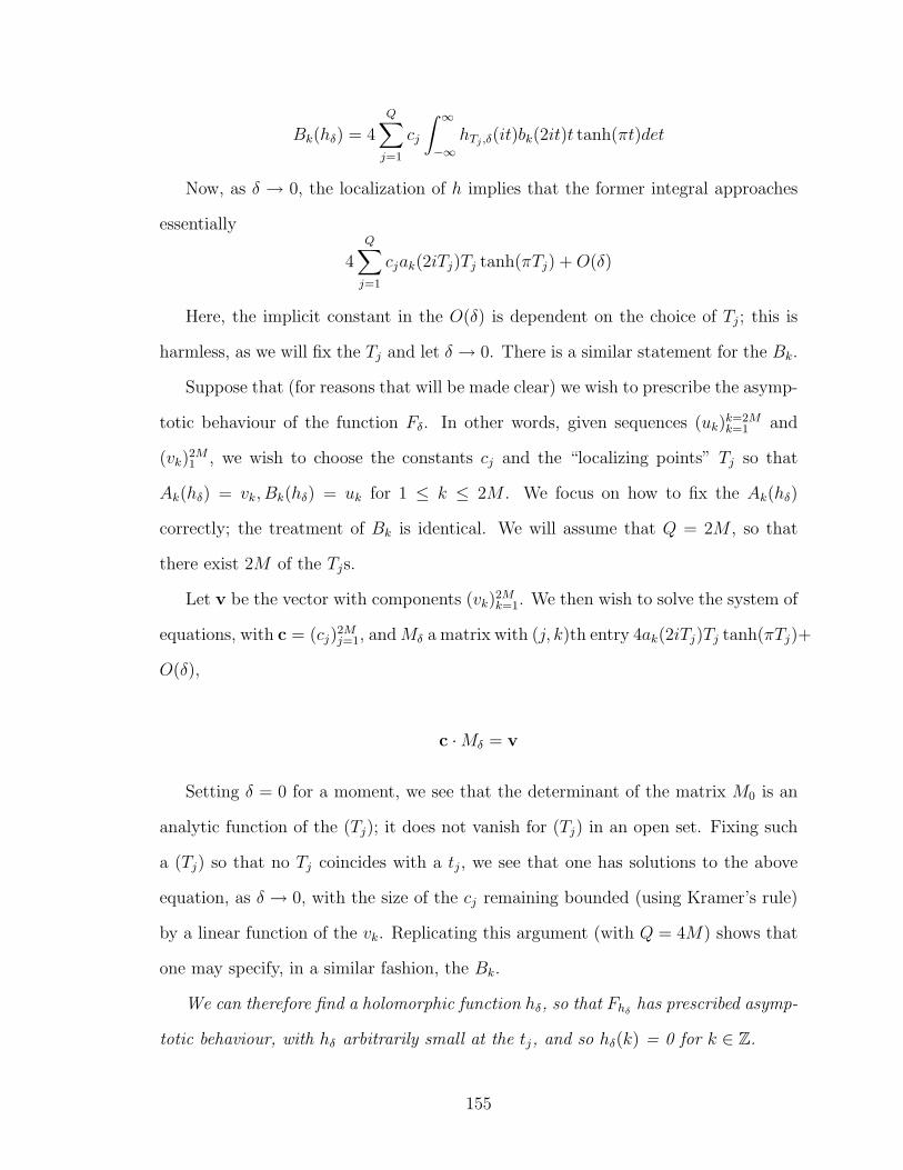
Bk(hδ) = 4
Q∑j=1
cj
∫ ∞
−∞hTj ,δ(it)bk(2it)t tanh(πt)det
Now, as δ → 0, the localization of h implies that the former integral approaches
essentially
4
Q∑j=1
cjak(2iTj)Tj tanh(πTj) +O(δ)
Here, the implicit constant in the O(δ) is dependent on the choice of Tj; this is
harmless, as we will fix the Tj and let δ → 0. There is a similar statement for the Bk.
Suppose that (for reasons that will be made clear) we wish to prescribe the asymp-
totic behaviour of the function Fδ. In other words, given sequences (uk)k=2Mk=1 and
(vk)2M1 , we wish to choose the constants cj and the “localizing points” Tj so that
Ak(hδ) = vk, Bk(hδ) = uk for 1 ≤ k ≤ 2M . We focus on how to fix the Ak(hδ)
correctly; the treatment of Bk is identical. We will assume that Q = 2M , so that
there exist 2M of the Tjs.
Let v be the vector with components (vk)2Mk=1. We then wish to solve the system of
equations, with c = (cj)2Mj=1, andMδ a matrix with (j, k)th entry 4ak(2iTj)Tj tanh(πTj)+
O(δ),
c ·Mδ = v
Setting δ = 0 for a moment, we see that the determinant of the matrix M0 is an
analytic function of the (Tj); it does not vanish for (Tj) in an open set. Fixing such
a (Tj) so that no Tj coincides with a tj, we see that one has solutions to the above
equation, as δ → 0, with the size of the cj remaining bounded (using Kramer’s rule)
by a linear function of the vk. Replicating this argument (with Q = 4M) shows that
one may specify, in a similar fashion, the Bk.
We can therefore find a holomorphic function hδ, so that Fhδhas prescribed asymp-
totic behaviour, with hδ arbitrarily small at the tj, and so hδ(k) = 0 for k ∈ Z.
155
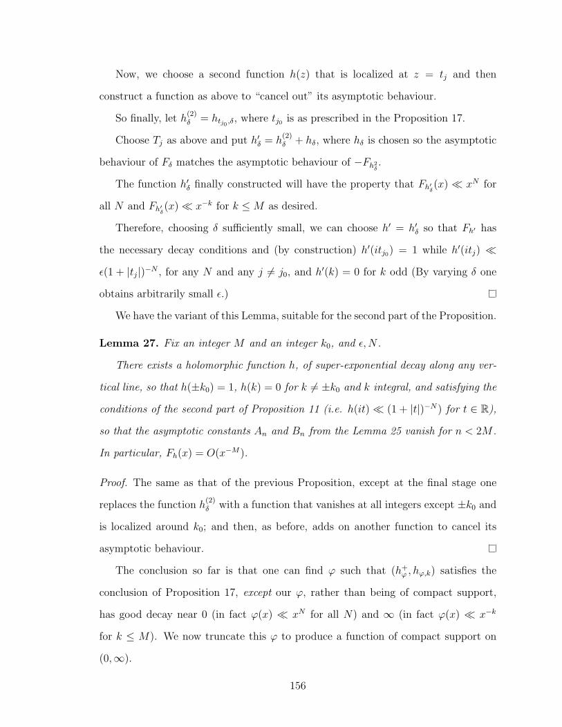
Now, we choose a second function h(z) that is localized at z = tj and then
construct a function as above to “cancel out” its asymptotic behaviour.
So finally, let h(2)δ = htj0 ,δ, where tj0 is as prescribed in the Proposition 17.
Choose Tj as above and put h′δ = h(2)δ + hδ, where hδ is chosen so the asymptotic
behaviour of Fδ matches the asymptotic behaviour of −Fh2δ.
The function h′δ finally constructed will have the property that Fh′δ(x) xN for
all N and Fh′δ(x) x−k for k ≤M as desired.
Therefore, choosing δ sufficiently small, we can choose h′ = h′δ so that Fh′ has
the necessary decay conditions and (by construction) h′(itj0) = 1 while h′(itj)
ε(1 + |tj|)−N , for any N and any j 6= j0, and h′(k) = 0 for k odd (By varying δ one
obtains arbitrarily small ε.)
We have the variant of this Lemma, suitable for the second part of the Proposition.
Lemma 27. Fix an integer M and an integer k0, and ε,N .
There exists a holomorphic function h, of super-exponential decay along any ver-
tical line, so that h(±k0) = 1, h(k) = 0 for k 6= ±k0 and k integral, and satisfying the
conditions of the second part of Proposition 11 (i.e. h(it) (1 + |t|)−N) for t ∈ R),
so that the asymptotic constants An and Bn from the Lemma 25 vanish for n < 2M .
In particular, Fh(x) = O(x−M).
Proof. The same as that of the previous Proposition, except at the final stage one
replaces the function h(2)δ with a function that vanishes at all integers except ±k0 and
is localized around k0; and then, as before, adds on another function to cancel its
asymptotic behaviour.
The conclusion so far is that one can find ϕ such that (h+ϕ , hϕ,k) satisfies the
conclusion of Proposition 17, except our ϕ, rather than being of compact support,
has good decay near 0 (in fact ϕ(x) xN for all N) and ∞ (in fact ϕ(x) x−k
for k ≤ M). We now truncate this ϕ to produce a function of compact support on
(0,∞).
156

Thus, let g be a smooth positive C∞ function on R of compact support, such
that g(x) = 1 for −1 ≤ x ≤ 1 and g(x) = 0 for x ≥ 2. If h is a function as in
Lemma 26 or Lemma 27, put ϕr(x) = Fh(x)g(log(x)r); the idea is that, as r → 0,
ϕr → ϕ pointwise, and it is a smoothly truncated version of ϕ with compact support
in (0,∞). In order to compare the transform of ϕr with ϕ one notes that ϕr − ϕ is
the sum of smooth functions ϕ1,r and ϕ2,r, where:
ϕ1,r supported in x ≤ 1 with growth εxN , for arbitrary N and ε → 0 as r → 0;
ϕ2,r is supported in x ≥ 1 and has growth εx−M+1, where again ε → 0 as r → 0.
(Note, one can introduce the ε by sacrificing a power in the exponent.) Finally, the
derivatives ϕ′1,r and ϕ′2,r satisfy the same estimates.
Now apply the following two estimates, Lemma 28 and Lemma 29. These show
that truncating ϕ in this fashion does not vary h “much.” In combination with the
previous Lemmas, they complete the proof of Proposition 17.
Lemma 28. Suppose ϕ is a smooth function supported in x ≤ 1, such that ϕ and
its derivatives ϕ(l)(x), for l ≤ N , satisfy ϕ(l)(x) m εxm for all m > 0. Then
h+ϕ (t) ε(1 + |t|)−N , and a similar estimate holds for hϕ,j with j odd.
Proof. One has the power series representation Jν(z) = zν∑
k(−1)k
k!Γ(k+1+ν)(z/2)2k. Let
Mϕ(s) =∫x>0
ϕ(x)xs−1dx be the Mellin transform of ϕ. The conditions on ϕ imply
that Mϕ(it) ε(1 + |t|)−l for l ≤ N .
We may write:
h+ϕ (t) =
1
2 sin(πit)Γ(1 + 2it)
((Mϕ(2it)−
Mϕ(2it+ 2)
1(1 + 2it)+
Mϕ(2it+ 4)
2!(1 + 2it)(2 + 2it)+ . . .
)
From this expression one obtains the required estimate. The expression for hϕ,k
follows similarly, replacing Jk(z) by the first few terms in its power series.
157

Lemma 29. Suppose ϕ is supported in x ≥ 1 so that, for 0 ≤ l ≤ k, ϕ(l)(x) εx−M
for some fixed M . Then hϕ,j εj−M and h+ϕ (t) ε(1 + |t|)−k+2.
Proof. (Sketch.) First we estimate for k odd
hϕ,k =
∫ ∞
0
ϕ(x)Jk(x)x−1dx
From the power series representation Jl(z) = ( z2)l∑∞
k=0(−1)k
k!(k+l)!( z
2)2k we see that, all
implied constants being absolute,
|Jl(z)| 1
l!(z
2)l
∞∑k=0
1
k!(z2
4l)k 1
l!(z
2)lez
2/4l
In particular,
Jl(αl) 1√l(αe1+α
2/4)l
Using this, we obtain that hϕ,k εk−M (one can essentially work out the integral
that computes hk by integrating from x = O(k) to ∞.)
We now wish to estimate h+ϕ (t). For this we use the Mellin-Barnes integral, for
0 < σ < 1,
J2it(x) =1
4πi
∫<(s)=σ
(x2
)−s Γ(it+ s/2)
Γ(1 + it− s/2)ds
In particular, we see that
h+ϕ (t) =
1
4πi sin(iπt/2)
∫<(s)=σ
2sMϕ(−s)Γ(it+ s/2)
Γ(1 + it− s/2)ds+ . . .
where we have only written out one of the two terms, and Mϕ(s) is the Mellin trans-
form of ϕ; it is analytic in a left half-plane, <(s) < M . Integration by parts shows
Mϕ(σ + ir) ε(1 + |r|)−k.
One obtains the estimate h+ϕ (t) ε(1 + |t|)−k+2. Indeed, take σ = 1/2, and write
158

s = 1/2+ ir, and use Stirling’s formula to estimate 1sin(iπt/2)
Γ(i(r+t)+1/2)Γ(1/2+i(t−r)) – it never gets
larger than O(|t|) as r varies, and this only happens for |r| |t|. Quantifying this
gives the required estimate.
6.4 Trace formulas
The purpose of this section is to indicate why a trace formula restricted over dihedral
forms – such as that derived in Chapter 2 – actually suffices to classify and construct
such forms. This is relatively standard, and we include a brief discussion, only for
completeness.
For simplicity we have always dealt with coefficients prime to the conductor; these,
in any case, suffice to determine the form, by strong multiplicity one. It is also
possible, with more effort, to carry through our technique for coefficients not prime
to the conductor.
Let N be an integer and χ a Dirichlet character to the modulus N . Suppose S
is a set of distinct Hecke eigenforms of conductor N and character χ, and denote as
usual by λn(f) the nth Hecke eigenvalue.
Proposition 18. Suppose that one is also given a set S ′ and, for each α ∈ S ′, a
sequence bαm which satisfies the Hecke relations relative to χ, so that for each α ∈ S,
bαmbαn =
∑d|(m,n)
bαmn/d2χ(d)
Suppose one is also given complex constants Cf for each f ∈ S and Cα for each
α ∈ S ′, and that the sequences bαm for α ∈ S are distinct (i.e. given α, α′ ∈ S ′, there
is m such that bαm 6= bα′m). Suppose also that:
∑f∈S
Cfλn(f) =∑α∈S′
Cαbαn
159

Then there is a bijection F : S ′ → S so that CF (α) = Cα, and λn(F (α)) = bαn for
n prime to N .
Proof. Indeed, let T be the abstract Hecke algebra generated by all Hecke operators
Tp, for p prime to N . (That is, the algebra of operators Tn, for (n,N) = 1, subject
only to the usual multiplication relations.) Associated to each f ∈ S is a natural one-
dimensional T-module Vf , on which Tn acts by λn(f). Similarly, to each bαn one can
associate a one dimensional T-module, Vα, so that Tn acts by bαn. The consequence
of our conditions is that the virtual T-modules ⊕f∈SCfVf and ⊕α∈S′CαVα have the
same characters; therefore, being semisimple finite-dimensional modules, they are in
fact isomorphic as virtual modules. This provides the result.
6.5 L-functions
6.5.1 Contour Shifting
The aim of this section is to describe the procedure for estimating partial sums of
coefficients of L-series, via contour shifting. This procedure is used throughout the
main text.
Suppose one has Dirichlet series L(s) =∑∞
n=1 ann−s and H(s) =
∑∞n=1 bnn
−s,
satisfying bounds an nA, bn nA; the series are then absolutely convergent in
<(s) > 1 + A.
Let g(x) be a C∞ function of compact support on (0,∞), with Mellin transform
G(s) =∫g(x)xs−1dx. Then g(x/X) has Mellin transformXsG(s). Now G(σ+it) N
(1 + |t|)−N , and we may write
∑n
ang(n/X) =
∫<(s)1+A
G(s)L(s)Xsds
In particular, if L(s) has analytic continuation up to <(s) = A′ in such a way that
160
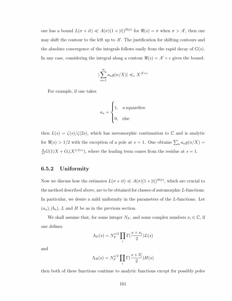
one has a bound L(σ + it) A(σ)(1 + |t|)B(σ) for <(s) = σ when σ > A′, then one
may shift the contour to the left up to A′. The justification for shifting contours and
the absolute convergence of the integrals follows easily from the rapid decay of G(s).
In any case, considering the integral along a contour <(s) = A′ + ε gives the bound:
|∞∑n=1
ang(n/X)| ε XA′+ε
For example, if one takes
an =
1, n squarefree
0, else
then L(s) = ζ(s)/ζ(2s), which has meromorphic continuation to C and is analytic
for <(s) > 1/2 with the exception of a pole at s = 1. One obtains∑
n ang(n/X) =
6π2G(1)X +Oε(X
1/2+ε), where the leading term comes from the residue at s = 1.
6.5.2 Uniformity
Now we discuss how the estimates L(σ+ it) A(σ)(1 + |t|)B(σ), which are crucial to
the method described above, are to be obtained for classes of automorphic L-functions.
In particular, we desire a mild uniformity in the parameters of the L-functions. Let
(an), (bn), L and H be as in the previous section.
We shall assume that, for some integer NF , and some complex numbers νi ∈ C, if
one defines
ΛF (s) = Ns/2F
∏i
Γ(s+ νi
2)L(s)
and
ΛH(s) = Ns/2F
∏i
Γ(s+ νi
2)H(s)
then both of these functions continue to analytic functions except for possibly poles
161

at s = 0, 1, and also ΛF (s) = αΛH(1− s), where α ∈ C with |α| = 1. We will assume
that the νi have absolutely bounded real part, that is, there is a fixed constant C so
that |<(νi)| ≤ C always.
From the functional equation,
L(s) = αN1/2−sF
∏i
Γ(1−s+νi
2)
Γ( s+νi
2)H(1− s)
We will derive certain estimates for L(s) which will make clear the dependence
on νi. Since the real parts of the νi are confined to a compact set, we are only really
varying their imaginary parts. Write = for imaginary part. Now one obtains easily,
for <(σ) ≥ 1/2.
Γ( (1−σ)+(νi+it)2
)
Γ(σ+(νi+it)2
)∏i
(1 + |=(νi) + t|)1/2−σ
In particular, for σ −A, one obtains, using the absolute boundedness of H(s) for
<(s) > A, that:
L(σ + it) N1/2−σF
∏i
(1 + |=(νi) + t|)1/2−σ
Let CF = NF
∏i(1 + |=(νi)|), the “analytic conductor.” It is now a consequence
of the Phragmen-Lindelof “convexity” principle that such a bound holds for any σ:
L(σ + it) CA(σ)F (1 + |t|)B(σ)
where the A(σ) and B(σ) are piecewise linear in σ, and absolute.
The following special case is important for the text; it follows from the results
of this Subsection and the previous one. Let f be a Maass cusp form of eigenvalue
1/4 + ν2 normalized to have L2 norm 1; then
∑n
g(n/X)af (n2) (1 + |ν|)AX
162

for some absolute constant A. This follows by applying the previous discussion to
the Dirichlet series∑
n af (n2)n−s, which is the quotient of the (finite part) of the
symmetric square L-function by ζ(2s). Actually, one obtains a still stronger result,
with a (possible) main term coming from the residue and a remainder term, but we
do not need that.
163
Notation Index
Since there are a very large number of symbols used in this thesis, we have tried
to here to give the section or subsection where many of them are first introduced.
Although it is not exhaustive, it will hopefully be of use in navigating this document.
There are various notations that are used across different Chapters; by and large,
they represent analogous concepts – for example, ∆ in Chapters 2 and 4. If a symbol
is used in multiple places in a given chapter, those usages are, if not identical, at least
compatible (e.g., one is a generalization of the other), unless explicitly otherwise
indicated below. The symbol listing for Chapter 5 is sparse, as that Chapter refers
explicitly to Chapter 4 for notation. We have omitted the Appendix.
1.2 π,m(π, ρ), L(s, π, ρ), λ(n, π, ρ).
1.3.1 an(f), λn(f), h(tf ).
1.4 ε, xε.
2.2 χ,N, Sχ(m,n, c), g,∑
n∼X .
2.2.1 an(f).
2.2.2 ηc, h±, hf (ϕ).
2.2.3 h±,∆.
2.3 D,χD, N, f, c(N),m.
164

2.3.1 k, L, ν,A(ν; c,m), δ(x).
2.3.2 oD,f , o(1)D,f ,S
′, δ, ε0, Xm, Xm, wf .
2.3.3 Z(s), Zp(s), g(p), β, εp, γp.
2.4 Lstandard, Sstandard.
2.5 K,K∞, ω,AK , CD,f , hD,f , U(f), Uv(f), fω, λm(fω), tω, εω, kω.
2.5.2 Cusp,Eis.
2.5.3 Class, Cg,B(g).
2.5.4 c0, c∞, Lcst,Λ(χ, s), L(χ, s), η′, H, H.
2.6 bαm.
3.1 L(s, f × σ).
3.2 bn, S(m;X), C, c(f), f , F, β,Diag.
3.2.1 gq(y), L(d, q; s),Λ(d, q; s), R(ρ), ρi, E.
3.2.2 h(x), fc(y), φ(c).
3.2.3 P(L(d, c, s)), r, ρ, R(ρ), Gc(s).
4.1 hF , DF , RF , A, CF , oF , d, F∞, F∞,+, v,R[F :Q],AF , AF,f , oF,v, ov, o∗F , o∗,+F , Fv, oF,f ,
oF,f×, UF,v,Uv,o
×F,v, πa, Norm, Z,N, ψ.
4.2 Γ0(I; a),Γ0(I), K0(I), K0,v(I), d−1, d.
4.2.1 π, χ, χ∞, χf , det,Xa,Funχ, δa, L2χ(I), L2
χ, Vχ′ .
4.2.2 σK , SO2(F∞), f , δ(α, β),Wφ0 ,Wφ0,∞,W∞, aunf , af (a, α), λf (q), Cf , ε.
4.3.1 K0, χK0 , CF , CF (2), S,K ′.
165

4.3.2 KSχ, hf , Jπ∞ , π(t, sgn), h(t), hϕ,∆.
4.3.3 I,DK/F , f, oK,I, q, α,m, g, µ,Σ,Σa,Σa,µ.
4.3.4 c, k,∼,Ψc,ε,Aa(ν; c, µ), || · ||, δa,∆,S,S′, σK , log, o′K,I, XK,a,(µ), XK,a,m.
4.4.1 φ, I(ν ′; c′, µ′).
4.4.2 ν ′, µ′, ν0, µ0, Zv,r, Zv(ωv, s), Z(ω, s), C.
4.4.3 fχ, f, fv, fχ,v, χν′2−4µ′ , Qv,Ms,M≥s, g(ωv, ψv), ε(ωv, ψv).
4.4.4 β, β1, β2, KQ, πK .
4.5 ω (this usage is essentially different to the usage in (4.4.2)),π(ω), I, UI,v, UI, U ,
ΛU , Λ′U , CK,I, CK,I;F , ∆, ∆′, Pl∞, ΛU,+, Λ′
U,+.
4.5.1 log, ω∞, tω, RK,I, RF , Xa,J.
4.6 G,N,B,N,A, Z, n(x), a(y1, y2), w, µI , µB, L2χ(Γ0(I; a)\GL2(F∞), ψ1, ψ2, fη,ν , Pη,ν ,
ZΓ, α, F (g), ΓP .
4.6.1 (Pη,ν)ψ,Ω, S(ω), KSχ(ω), ηψ−12, ϕ,KSχ(ψ1, ψ2, c, ε).
4.6.2 Projπ,Wπ,ψ,Wφ,ψ, 〈, 〉W , c(π, ψ1), Fπ(fη,ν), Jπ,ψ, β, c(π : ψ1 → ψ2).
4.6.3 aunf , anmf .
5.2 Ap, λπ(n), E(s).
5.3 ρπ, q, Nχ(q),B, λf (p)
5.3.1 I (denotes a generic ideal, as distinct from usage in Chapter 4),aIcoI , T,N .
166
Bibliography
[1] R. W. Bruggeman and R. J. Miatello. Estimates of Kloosterman sums for groups
of real rank one. Duke Math. J., 80(1):105–137, 1995.
[2] R. W. Bruggeman and R. J. Miatello. Sum formula for SL(2) over a number
field and Selberg type estimate for exceptional eigenvalues. Geom. Funct. Anal.,
8(4):627–655, 1998.
[3] Daniel Bump. Automorphic forms and representations. Cambridge University
Press, Cambridge, 1997.
[4] James W. Cogdell and Ilya Piatetski-Shapiro. The arithmetic and spectral anal-
ysis of Poincare series. Academic Press Inc., Boston, MA, 1990.
[5] W. Duke. The dimension of the space of cusp forms of weight one. Internat.
Math. Res. Notices, (2):99–109 (electronic), 1995.
[6] W. Duke, J. B. Friedlander, and H. Iwaniec. Bounds for automorphic L-functions,
III. Invent. Math., 143(2):221–248, 2001.
[7] Stephen Gelbart and Herve Jacquet. A relation between automorphic represen-
tations of GL(2) and GL(3). Ann. Sci. Ecole Norm. Sup. (4), 11(4):471–542,
1978.
[8] I. S. Gradshteyn and I. M. Ryzhik. Table of integrals, series, and products.
Academic Press, New York, 1965.
167
[9] Erich Hecke. Mathematische Werke. Vandenhoeck & Ruprecht, Gottingen, third
edition, 1983. With introductory material by B. Schoeneberg, C. L. Siegel and
J. Nielsen.
[10] Henryk Iwaniec. Introduction to the spectral theory of automorphic forms. Re-
vista Matematica Iberoamericana, Madrid, 1995.
[11] N. V. Kuznetsov. The Petersson conjecture for cusp forms of weight zero and the
Linnik conjecture. Sums of Kloosterman sums. Mat. Sb. (N.S.), 111(153)(3):334–
383, 479, 1980.
[12] J.-P. Labesse and R. P. Langlands. L-indistinguishability for SL(2). Canad. J.
Math., 31(4):726–785, 1979.
[13] R. Langlands. Beyond Endoscopy. To appear (Preliminary version online at
http://www.sunsite.ubc.ca/DigitalMathArchive/Langlands).
[14] Hans Maass. Uber eine neue Art von nichtanalytischen automorphen Funktionen
und die Bestimmung Dirichletscher Reihen durch Funktionalgleichungen. Math.
Ann., 121:141–183, 1949.
[15] P. Michel and A. Venkatesh. On the dimension of the space of cusp forms
associated to 2-dimensional complex Galois representations. IMRN, to appear.
[16] Shin-ichiro Mizumoto. On the second L-functions attached to Hilbert modular
forms. Math. Ann., 269(2):191–216, 1984.
[17] P. Sarnak. Letter to R. Langlands. personal communication.
[18] Siman Wong. Automorphic forms on GL(2) and the rank of class groups. J.
Reine Angew. Math., 515:125–153, 1999.
168