Proceedings of the Workshop on Economics of Road Design StandardsBureau of Transport Economics, ISBN 0 642 05703 6, 9780 642 05703 7

Australian Government Publishing Service, 1980

ECONOMIC ANALYSIS AND OPERATIONSRESEARCH TECHNIQUESIN THE SELECTION OF ROAD DESIGNPARAMETERSKeith Linard, Director Special Studies Branch and

S. Gooneratne, Project Engineer

Bureau of Transport Economics, Canberra

(Revised & Updated May 2014)

TABLE OF CONTENTS

TABLE OF CONTENTS......................................................................................................................................................... 2

LIST OF TABLES.................................................................................................................................................................. 3

LIST OF FIGURES................................................................................................................................................................ 4

ABSTRACT.......................................................................................................................................................................... 5

Scope & Purpose ............................................................................................................................................................... 5

Decision Contexts, Decision Rules & Decision Criteria in Economic Evaluation............................................................... 6

Decision Contexts.......................................................................................................................................................... 6

Perception of Funding Constraints ........................................................................................................................... 7

Decision Criteria ........................................................................................................................................................ 7

The Decision Rule for Specific Contexts.................................................................................................................... 9

Choice of Discount Rate ............................................................................................................................................ 9

Case Studies: Decision Contexts in relation to Road Design Standards........................................................................... 9

Selection of Optimum Geometric Road Design Parameters (Cases 1, 2 AND 3) ........................................................10

General Formulation...............................................................................................................................................10

Case 1: Optimum Geometric standards under unconstrained funding..................................................................11

Case 2: Funding constrained both to K dollars per period and to M periods.........................................................12

Case 3: Funding is constrained to K dollars, per period but available until program of L project units is completed.................................................................................................................................................................................12

Possible Relevance of Cases 2 and 3 to National Highway and Rural Arterial Programs ...................................14

Design Standards & Mathematical programming of Highway Investments...............................................................17

Case 4: A Programming Formulation of an Investment Program with Stage Construction, Alternative DesignStandards and Multi-Period Budget Constraints ....................................................................................................17

Computing Costs .................................................................................................................................................19

Advantages of Mathematical Programming .......................................................................................................19

Iterative Procedures............................................................................................................................................19

Traffic Congestion Costs and Capacity Standards – Justification for Capacity Standards ..................................20

Case 5: Optimal timing of capacity improvements.................................................................................................21

Case 6: Decisions Concerning Design Floods ..........................................................................................................23

Maximising Net Present Value............................................................................................................................23

Expected Utility Criterion....................................................................................................................................23

Multiple Objective Criteria..................................................................................................................................24

Dealing with Risk and Uncertainty ......................................................................................................................26

The Safety Objective Function ............................................................................................................................26

Case 7: Cost-effectiveness methodology................................................................................................................28

Overview of Cost-Effectiveness Analysis ............................................................................................................28

Decision Rules for Cost-Effectiveness Analysis ...................................................................................................30

Average Cost-Effectiveness Ratio (ACER)............................................................................................................30

Incremental Cost-Effectiveness Ratio .................................................................................................................30

Conclusion.......................................................................................................................................................................34

Appendix A: Abbreviations & Subscripts Used in Figure 5.............................................................................................35

Appendix B: Alternative Definitions of Benefit-Cost Ratio ............................................................................................36

Appendix C: Equations Giving Optimum Capital Outlay and Optimal Geometric Design Standard for Cases 1, 2 & 3 .37

Case 1: Optimum Geometric standards under unconstrained funding - L, N & r are constants - unconstrainedbudget scenario ..........................................................................................................................................................37

Case 2: Funding is constrained both to K dollars per period and to M periods - K, M, N & r are constants; k andb=f(k) are variables .....................................................................................................................................................37

Case 3: Funding is constrained to K dollars, per period but available until program of L project units is completed -L, K, N & r are constants; k, f(k) are variables .............................................................................................................38

Appendix D: Decision for Mutually Exclusive Projects with & Without Budget Constraints .........................................39

Graphical Derivation of Results...................................................................................................................................39

Unconstrained Budget ................................................................................................................................................39

Constrained Budget with Shadow Price ..................................................................................................................39

REFERENCES ....................................................................................................................................................................41

LIST OF TABLES

Table 1: Decision Rules for Various Economic Optimisation Criteria & Relevance to Decision Contexts ........................ 8Table 2: Actual Investment Benefits compared with Corresponding Community Priorities..........................................26Table 3: Ranking of Road Safety Countermeasures by Decreasing Cost-Effectiveness (Present Value ofCountermeasure per Total Fatalities Forestalled over 10 Years.....................................................................................27Table 4: Cost-Effectiveness Ratio of Independent Safety Improvements According to Different Decision Criteria(Maximands) ...................................................................................................................................................................29Table 5: Data for Cost Effectiveness Analysis of Mutually Exclusive Options (Hume Circle).........................................31Table 6: Three Step Incremental Cost Analysis of Hume Circle Options ........................................................................33

LIST OF FIGURES

Figure 1: Variation of Capital Cost with Increasing Design Standards ............................................................................10Figure 2: Variation of Benefits per Period with Project Capital Cost..............................................................................11Figure 3: Optimum Gradient versus Rate of Funding for Reconstruction of Twenty 1.6km Road Segments (SourceMcLean 1976)..................................................................................................................................................................13Figure 4: NPV versus Capital Cost for a single 1.6km Road Segment .............................................................................14Figure 5:Cumulative Expenditure by Benefit Cost Ratio (BCR) for All National Highways by State & Territory ............15Figure 6: Cumulative Expenditure versus Benefit Cost Ratio (BCR) by State for Rural Arterials ....................................16Figure 7: Travel Time versus Hourly Traffic Volume .......................................................................................................20Figure 8: Travel Time Savings versus Hourly Traffic Volumes.........................................................................................21Figure 9:Net Present Value versus Commissioning Year ................................................................................................22Figure 10: Present Value of Benefits versus Present Value of Costs showing - Illustrating Lower Optimum Capitalwhen Budget is Constrained to....................................................................................................................................23Figure 11: Utility Function of Risk Averse Decision Maker .............................................................................................24Figure 12: Capital Cost of Bridge versus Deck Level .......................................................................................................25Figure 13: Average Annual Time of Bridge Pavement Submergence .............................................................................25Figure 14: Incremental Cost Effectiveness Analysis for Mutually Exclusive Options - Equivalent Annual Cost versusAccident Reduction Benefits ...........................................................................................................................................32Figure 15: Correctly defining the Benefit Cost Ratio ......................................................................................................36Figure 16: PVB versus PVC for Mutually Exclusive Projects OA, OB, OC & OD ...............................................................40Figure 17: NPV versus PVC for OA, OB, OC & OD...........................................................................................................40

ECONOMIC ANALYSIS AND OPERATIONSRESEARCH TECHNIQUES IN THESELECTION OF ROAD DESIGNPARAMETERSKeith Linard, Director Special Studies Branch and S. Gooneratne, Project Engineer,Bureau of Transport Economics, Canberra

ABSTRACT

One purpose of design standards is to serve as a substitute for the need for repeated selection ofoptimal design parameters. For many situations this is a legitimate use of standards in road designand construction as in other fields of engineering. However, it is suggested that for certain majorprojects and in extreme conditions of terrain or climate it is highly desirable that the selection ofimportant design parameters be assisted by economic analysis and relevant operations researchtechniques.

Several classes of design standards are considered and an optimisation methodology is set out foreach class, taking into account the constraints, the decision contexts, the decision criterion and therelated decision rule. Some examples are given to illustrate the procedures, and their advantagesand limitations are discussed.

Scope & Purpose

The primary purpose of this paper is to draw attention to and provide an outline of the methodologyfor economic optimisation of road design parameters. The methodology is specifically related tosome of the decision contexts in the Consolidated Set of Design Standards for National Highways inAustralia but the basic principles are applicable in most other situations.1

This paper should not be necessary, given the many general texts on economic optimisationtechniques published in recent decades and the considerable literature on economic evaluationdisseminated by bodies such as the Commonwealth Treasury, the Bureau of Transport Economicsand the former Commonwealth Bureau of Roads.2 Unfortunately, in all areas of public sectorinvestment analysis, both in Australia and overseas, the technical quality of many economic analysesleaves much to be desired, principally because authors appear not to appreciate that differentdecision contexts require different decision rules. Also, the literature is sparse on the application ofeconomic optimisation techniques specifically to the selection of road design parameters. Some ofthe few useful contributions will be discussed later, in the appropriate contexts.

We are not arguing that economic optimisation should be the sole, or even the principal, criterion inthe selection of design standards. It is our contention, however, that it is a very important input andshould not be lightly ignored. Nor are we arguing that detailed economic evaluation of design

1 Consolidated Set of Design Standards for National Highways in Australia, Australia (1976).These design standards were declared in September 1976 by the Minister for Transport underprovision the National Roads Act 1974.2 Examples are Dasgupta and Pearce (1978), Mishan (1971), de Neufville and Stafford (1971),Cassidy and Gates (1977) and Reutlinger (1970).

standards is necessary in all cases. For most purposes, professional judgement guided by designmanuals and informed through State road authority and other local and international road researchprovides an appropriate basis for the selection of design parameters. We do consider, however, thatthere are frequent situations where professional judgement can and should be assisted bytechniques based on economic evaluation, cost effectiveness analysis and systems analysis.Situations where this may be desirable at the design level include major road projects such as townby-passes, decisions concerning rural freeways and specific projects through difficult terrain andflood-prone areas. Of course, we consider it axiomatic that the actual preparation of standards andtechnical guides be guided, inter alia, by economic considerations.3

Decision Contexts, Decision Rules & Decision Criteria in Economic Evaluation

As discussed by Taplin (1980) and Latham (1980) there are multiple objectives relevant to decisionson road standards. In this paper we are concerned solely with the economic objective function. Theeconomic objective function or the economic maximand to be pursued is the expected net presentvalue of the available set of investment opportunities. That is, for any given decision context, thedecision rule relating to economic optimisation should be consistent with maximising the expectednet present value of the investment.

Unfortunately considerable confusion exists both in the literature and amongst practitioners when itcomes to translating this decision rule into practice. This confusion stems in part from a failure todistinguish between the decision criterion and the decision rule, and from a failure to recognise thatdifferent decision contexts may require different decision rules. This failure to distinguish betweenthe criteria and the decision rules applicable to the criteria can and does lead to confusing andsometimes erroneous outputs.

The considerable, often conflicting, literature on the relative merits of different criteria such as netpresent value (NPV), benefit-cost ratio (BCR) and internal rate of return (IRR) is largely a result of thisfailure.4

Decision Contexts

For the present purpose the broad categories of decision situations confronting public sectoranalysts may be classified as follows:5

i. Accept-Reject - No Budget Constraint: Faced with a set of independent projects and noconstraint on the number which can be undertaken, the analyst is required 'to identify all'worthwhile' projects.

ii. Accept-Reject - Constrained Budget: Faced with the analysis of one specific project inisolation of the total sector program, and given that sectoral budget constraints exist, theanalyst is required to determine whether an identified solution is 'worthwhile'.

iii. Choice Between Mutually Exclusive Projects: Where projects are interdependent or mutuallyexclusive (e.g. alternative geometric standards or alternative alignments for a given sectionof road) the analyst is required to identify the 'best' alternative, assuming either:

3 It is encouraging that the recent revision (NAASRA, 1979) to policy for Geometric Design ofRural Roads (NAASRA, 1976) has been approached in this manner and that the current edition ofAustralian Rainfall and Runoff (Institution of Engineers, Australia, 1977) provides no prescriptiveflood design standards, reversing its previous policy.4 See for example the debate in Engineering Economist on the relative merits of IRR indifferent contexts.5 See also Dasgupta and Pearce (1978, p.160).

a) no budget constraint as in (i), or:

b) constrained budget, as in (ii)

iv. Selection of Optimal Project Size or Time Phasing (Staging): This is a special case of (iii).

v. Selection of Optimal Replacement Cycle: This is a special case of (iii).

vi. Program Composition - Single Period Rationing: Where capital is constrained for a singleperiod, the analyst is required to determine, from a given list of possible independentprojects, the composition of and relative priority within an investment program.

vii. Program Composition - Multi-Period Rationing: Where there are multi-period constraints oncapital or other resources, the analyst is required to determine, from a given list of possibleindependent projects, the composition of and relative priority within an investmentprogram.

In decision contexts of type (vi) and (vii), the projects considered are often not all independent. Thetreatment of program composition where some projects or groups of projects are mutually exclusiveis discussed in the text.

In carrying out an economic analysis, correct specification of the decision context is of utmostimportance. If the context of an analysis is not properly specified, then the results of subsequentevaluations are likely to be irrelevant.

Perception of Funding ConstraintsThe decision contexts above refer to both constrained and unconstrained budget situations. Inpractice road funding has always been constrained. However, the perception of such constraints inrelation to the standards adopted for particular situations appears to diminish with the remotenessof the decision maker from construction and maintenance activity. It is perhaps partly a result of thisthat in both Australia and the US, the design codes up to the mid-1970s evidenced little perceptionof economic constraints and were based largely on considerations of engineering excellence.

Decision CriteriaA wide range of criteria are used in practice for economic evaluation: net present value (NPV), thebenefit-cost ratio (BCR), the internal rate of return (IRR), marginal present value (MPV), marginalbenefit cost ratio (MBCR), and capital efficiency ratio (CER) are the most common. Appendix Adefines each criterion.

The NPV criterion is always appropriate to use in determining the optimum economic solution. TheBCR is appropriate in certain specific circumstances, but is not synonymous with maximising netpresent value in a number of common situations, especially when applied to mutually exclusivealternatives (de Neufville and Stafford 1971; Gould 1972). The IRR criterion, even when properlyapplied (and it is almost invariably used incorrectly) can and generally will result in an incorrecteconomic decision6. Gould (1972) demonstrates that the IRR is totally irrelevant to decision makingon mutually exclusive alternatives, the context, paradoxically, where it is most often applied. TheCER is merely a variant on the benefit cost ratio (CER = BCR-1), and suffers from the defects of theBCR. The marginal present value and marginal BCR have limited applicability, but are very valuable inrelation to choice between mutually exclusive alternatives.

6 Cassidy and Gates (1977) argue that IRR is an invalid criterion in any context. In like manner,we contend that, while it does give the same answer as the NPV criterion in context (i), its useshould be avoided even then.

Table 1: Decision Rules for Various Economic Optimisation Criteria & Relevance to Decision Contexts

Note: = Shadow price of the budget, which is approximately the BCR of the most marginal (least worthwhile) project on the program.

The Decision Rule for Specific ContextsTable 1 details the decision rules appropriate to the different contexts outlined above. A list ofdefinitions of abbreviations used in the table is in Appendix A. More detailed discussion is containedin the texts referred to previously.

Choice of Discount RateThe discount rate serves to bring project alternatives with different time streams of costs or benefitsto a common basis as present value dollars. It is beyond the scope of this paper to discuss what theappropriate discount rate might be. However, as will be seen from some situations discussed later,the discount rate may be a critical parameter having a significant influence on the investmentdecisions being made.

Case Studies: Decision Contexts in relation to Road Design Standards

For purposes of illustration of how economic evaluation, cost­ effectiveness analysis and systemsanalysis may be applied we have selected the following decision contexts. The choice of an optimumstandard is, by itself, always a choice between mutually exclusive alternatives. However, othercontexts arise for example in staging of standards.

Case 1: Selection of optimum geometric road design standard given an unconstrained budget. Thedecision context in this case is of type (iii) in Table 1; choice is between mutually exclusive alternativestandards.

Case 2: Optimum geometric standard for progressive upgrading reconstruction of a highway systemgiven a multi-period budget constrained to K dollars for each of M periods. Choosing thecomposition and relative priority of individual projects, or 'project units' within the programconstitutes a decision context of type (vii). For the present purpose, however, we assume that thesequence of project units has been pre-determined or is given, and the decision required is that ofselecting the geometric standard to be adopted, such as the parameters defining the pavementwidth characteristics. The decision context is again of type (iii).

Case 3: The decision context in this case is similar to the previous one, and of the same type, withthe difference, that funding at K dollars per period ceases when all project units in the program toreconstruct the highway are completed.

Case 4: Selection of composition and relative priority of projects for stage construction of a corridorgiven multi-period rationing as described in Case 2. The decision context is type (vii). It is shown thatdesign standards for each stage could be optimised even though staging itself is a process ofoptimising a road design over the planning horizon.

Case 5: Optimal timing of road capacity improvements. The decision context is of type (iv) where thechoice is between alternative times for commissioning the improvement. As shown presently thisdecision can also be stated in terms of the traffic flow at which it is optimal to upgrade.

Case 6: Hydraulic design of a road section or structure. Again this is the context, type (iii), of a choicebetween mutually exclusive alternatives, but the stochastic nature of flood recurrence and thedisruptive effects of floods require different treatment from the previous examples.

Case 7: Maximising road safety. The context here is choosing the most cost-effective strategy tomaximise road safety given (a) a set of independent alternatives, and (b) a set of mutually exclusivealternatives. This context is included because it illustrates how the introduction of non-economicobjectives might be treated.

Selection of Optimum Geometric Road Design Parameters (Cases 1, 2 AND 3)

General FormulationWe assume the progressive reconstruction of a length L equal segments of a highway is to occur byspending a total capital of K dollars per period for M periods.

Although the geometric design standard of a road needs speed, width, curve radius and gradeparameters for its specification, let us denote by the variable S a set of any one or more of theseparameters. The capital cost kn dollars of construction or reconstruction of a single project unit (e.g.1 km section) is related to its geometric design standard S by a curve of the form shown in Figure 1.Since the curve is monotonically increasing, kn is a measure of the general design standard. If anoptimum value k1 of kn could be found, the corresponding best set s1 of geometric design parametersis also an optimum set for all values of k.

Figure 1: Variation of Capital Cost with Increasing Design Standards

We now make the strong assumption that the annual benefits $bn from each project segmentremains constant over time to t = N and that $b is the same for successive project units until all Lunits are completed. This implies that there is no traffic generated by the improvement and noincreasing returns to scale. Implications of this assumption and its partial relaxation are discussedlater.

As defined previously, $b includes both user benefits and changes in operating and maintenancecosts directly attributable to the project segment and is considered a function b = f ( k ) only of unitproject cost k and hence the design standard. With some encouragement from McLean (1976, Figure13), we venture to suggest that f( k ) will mostly be of the form shown in Figure 2. It is argued that

this curve will peak and then decline because increasing per unit maintenance costs and possiblyaccident costs7 will eventually outweigh marginal increases in user benefits.

We assume a discount rate of i = ( r – 1 ), and an analysis interval of N periods from t=0 to t=N whereN >= M. The derivation of solutions giving optimal k (and hence optimal design standards) for thethree different funding contexts of Cases 1, 2 and 3 is presented in Appendix B.

Case 1: Optimum Geometric standards under unconstrained fundingAlthough unconstrained funding is an inappropriate context for most road funding situations, wepresent the solution because it indicates that the highest possible design standard is not the bestchoice even with unlimited funds. This context may also be useful to consider the design standardappropriate for a very low volume rural highway which has relatively large funds available for itsreconstruction due to its high functional classification; for example, National Highways in veryremote parts of Australia.

The optimum solution, derived in appendix B, is given by the equation:

F’( k ) = ln(r) / (1 - r –N ) ≈ i (1)

The interpretation of this is surprisingly simple in that it is represented in Figure 2 by point C whosetangent has a slope for all practical purposes equal to the discount rate i. The standard C will belower than the standard D, the maximum standard level, since the discount rate will not approachzero. In other words, the optimum design standard is a function of the discount rate. Use of a lowerdiscount rate would result in a higher optimum design standard, as would be expected.

Figure 2: Variation of Benefits per Period with Project Capital CostA, B & C are solutions given optimum design standards in different decision contexts

7 There is some evidence, for example, that increasing the pavement width of a 2-lane, 2-wayrural road beyond 6.8 metres results in an increase in the accident rate. (See McLean 1980 and Dartand Mann 1970.)

Case 2: Funding constrained both to K dollars per period and to M periodsOne of the situations to which this context corresponds might be where a road funding program ofK * M dollars in total has been announced to be made available at the rate of K dollars per period forM periods. This would largely correspond to the present situation with regard to rural arterial roadprograms or the Roads to Recovery Program. The context outlined previously assumes that thebacklog of works is such that there are a large number of projects which have similar benefits perunit length - as will be discussed, this situation appears valid in a wide variety of cases.

In general, funds are known to be insufficient to reconstruct all of the L project segments (at $k persegment) of highway), that is

L > K * M / k (2)

As shown in Appendix B, the optimum design standard set is given by

k * f’( k ) - f( k ) = 0 (3)

This is represented by point A on Figure 2, the tangent which also passes through the origin. Thissolution corresponds to maximising the ratio of ( b / k ) as defined previously and, somewhatsurprisingly, it is independent of the discount rate i, the rate of funding, K dollars per period, thenumber of periods of funding M and the analysis period N.

What this solution means is that, provided the warranted or feasible project set cannot becompleted with the known or likely funding program, the optimum design standards set is thatwhich maximises ( b / k ), the ratio of user benefits less operating and maintenance costs per periodper project unit to capital cost per project unit. This result greatly simplifies the task of identifyingthe optimum standards for a road program which satisfies our assumptions. The optimum standardsfor the project unit considered in isolation correspond to the optimum program standards.

As shown in Appendix B, relaxing the assumption of constant benefits does not affect the optimalitycondition in equation (3) provided that the function relating benefits to time is of the form Mb(t) = b * h(t) . This implies that the ratio of benefits less operating and maintenance costs fromdifferent design standards remains constant over time. The possible applications of these results arediscussed after Case 3.

Case 3: Funding is constrained to K dollars, per period but available until program of Lproject units is completed

This context corresponds to the situation where a funding program exists at a specified rate of Kdollars per period until the completion of a specified program, following which the funding isassumed not to be switched to other road programs. This might correspond, for example, to aspecial program for a specific set of roads to assist a developing industry, for example the ‘Roads toRecovery’ program.

The number of periods M for which funding is available, for given L and K, now depends on k andhence the design standard adopted. As shown in Appendix B, the optimum solution for k is

{ k * ( 1 – r -pk ) - k 2 * p * ln(r) * r -N } * f’ ( k ) + { ( 1 – p * k *ln(r) * r -pk – 1 } * f( k )

- ln(r) * ( 1 – p * ln(r ) * r -pk ) = 0 (4 )

This is admittedly difficult to interpret at first sight. It could however be readily solved for k provided( b = f( k ) ) is known graphically. A very small computing effort is all that needed to solve equation(4) by a process of iteration.

Despite its foreboding appearance, equation (4) does suggest some interesting points. The optimumk depends on discount rate i, the ratio ( p = L / K ) and the analysis period N. The dependence on( L / K ) means that as the number L of project units or the magnitude of the program task isincreased, the funding rate K must increase proportionately to maintain the same optimum designstandard.

Using equation (4), it is possible to confirm McLean's graphical demonstration (McLean 1976) thatthe optimum design standard decreases as the rate of funding decreases. Taking a design gradeexample where the necessary detailed data was reported by Read (1971), and using the values L =20, i = ( r - 1 ) = 0.1 and N=30, McLean demonstrated that, with a decreasing rate of funding K and anincreasing number of years M = L * k/ K to program completion, the optimum maximum gradeincreases, that is, the optimum grade standard and K decrease, as shown in Figure 3 (McLean’sFigure 12 on p.27).

Figure 3: Optimum Gradient versus Rate of Funding for Reconstruction of Twenty 1.6km Road Segments(Source McLean 1976)

In Figure 4 (McLean's Figure 13), McLean plots NPV versus k for a single project unit. Obtaining f( k )graphically from this curve and iteratively solving equation (4), we could obtain an approximation ofMcLean’s curve of optimum design standard versus K and M which we have reproduced in Figure 3.This example demonstrates the value of equation (4) in road investment planning situations wheref( k ) can be graphically determined.

Figure 4: NPV versus Capital Cost for a single 1.6km Road Segment

Possible Relevance of Cases 2 and 3 to National Highway and Rural Arterial Programs

The above results are applicable where the assumptions concerning the constancy of benefitsremain valid. In general, this assumption is reasonable for two lane rural roads where congestioncosts are negligible and where there remains a large backlog of warranted projects. For example,congestion costs are negligible where traffic volumes in the design year are less than about 1800vehicles per day and where heavy vehicles constitute less than about 10% of the traffic stream. Thetraffic volume assumption is not restrictive, since at least two-thirds by length of the rural arterialand National Highway system carries less than 1800 vpd.

A measure of the change of benefits for successive increments in investments is afforded by thecurves in Figures 5 and 6 which show plots of Cumulative Expenditure versus BCR for NationalHighways and rural arterials respectively in different States.

The rate of change of benefits is least in the steepest portions of the curves. The figures suggest thatthe constancy of benefits assumption in the foregoing analysis is reasonably satisfactory in theinvestment range likely over the next decade in relation to National Highways in the NorthernTerritory, South Australia, Tasmania and Western Australia, whereas New South Wales is aborderline case. For rural arterials the assumptions are satisfactory in Victoria, Tasmania and SouthAustralia but in the case of Tasmania and Victoria the BCRs of these projects are less than 1.

Figure 5:Cumulative Expenditure by Benefit Cost Ratio (BCR) for All National Highways by State & Territory(All Horizontal Axes – Increasing BCR from Left to Right)

Figure 6: Cumulative Expenditure versus Benefit Cost Ratio (BCR) by State for Rural Arterials(All Horizontal Axes– Increasing BCR from Left to Right)

Design Standards & Mathematical programming of Highway Investments

Previous applications of mathematical programming to optimisation of highway investments havebeen described by de Neufville and Mori (1970) and Bowyer (1976). Bowyer also gives the mixed­integer linear programming formulation of an investment program consisting of s route segmentseach with L projects for implementation over T periods each of which has a constrained budget. Theformer Commonwealth Bureau of Road's system for its solution with a continuous phase followed bya branch and bound algorithm is described in detail by Bowyer.

A variable increment dynamic programming approach is used by de Neufville and Mori to obtain anoptimum schedule of investments for a program of investments including stage construction optionson some projects. Detailed formulation is not given, but an example is used to illustrate thesuperiority of their procedure to scheduling by benefit-cost ratios with budgetary constraints and bya static, period by period procedure. There appear to be no cases reported of solving or evenformulating an investment scheduling problem including the choice of alternative design standardsfor each project or each stage of a project. Such a formulation is given in Case 4.

Case 4: A Programming Formulation of an Investment Program with Stage Construction,Alternative Design Standards and Multi-Period Budget Constraints

Berry (1979) and Berry and Both (1980) describe the advantages of stage development and use ofalternative design standards in investment planning for the Victorian rural arterial road systemthrough examples at the network, corridor and project levels.

The following is an integer linear programming formulation of this problem. The context is similar tothat described by Forbes and Womack (1976) as it applies to highway planning in California.

We consider P sections of a corridor with Q construction stages in each section, thus generatingP * Q possible projects. Each project could be built to S alternative design standards commencingconstruction in any one of T periods. These sets define a set of four-dimensional variablesX( p, q, s, t ) representing the proportion of stage q of section p to be built to design standard s inyear t. If the projects are all indivisible, then:

X( p, q, s, t ) = 0 or 1, for all p, q, s, t ( 5)

From previous evaluations, the NPVs of all projects are determined and represented by V( p, q, s, t ).Project capital costs, K( p, q, s, t }, are expressed in constant prices. The objective function thenbecomes: = ∑ ∑ ∑ ∑ , , , × , , , (6)

Subject to the constraints:∑ ∑ ∑ , , , × , , , ≤ (7)

∑ ∑ ( , , , ) ≤ , (8)

∑ , + , , ≤ ∑ × , , , , , = 1 − 1 (9)

And: , + , , = , + , , × , , , + , + , , × ( − , , , ) (10)

For all p, s, t and q = 0 to Q – 1; X(p, 0, s, t ) = 0 for all p, s, t

And K1 is defined for q = 1 to Q – 1 and K2 for q = 0 to Q - 1

Equation (7) specifies the multi-period budget constraint. Equation (8), the mutual exclusivityconstraint, specifies that each project can be commenced only in any one period and to one designstandard. Equation (9) ensures that stage (q + 1) of a section cannot be scheduled before theprevious stage q and equation (10) selects project costs K from one of two cost matrices Kl and K2

depending on whether the previous stage of the same section was commenced at the same time orbefore, respectively. This last condition is needed if economies of scale exist in undertakingsimultaneous construction of any two successive stages of the same section.

The above formulation assumes in equation (7) that all capital funds for each project ( p, q, s, t )selected are allocated from the budget K(t) in the period of commencement. Alternatively, we maywish to specify, as Bowyer (1976) has done, that allocation for each selected project may come frommore than one period.

If, for example, the project allocation comes from two periods, a project commenced in period t hascapital costs Ka (p, q, s, t ) and Kb ( p, q, s, t+1 ) in periods t and t+1 respectively. Therefore thebudget K(t) in period t will fund Kb type costs of projects commenced in the previous period and Ka

type costs of projects commenced in period t. Hence the new budget constraint equation to replaceequation (7) becomes:

∑ ∑ ∑ , , , × , , , − + ∑ ∑ ∑ , , , × , , , ≤ ( ) (11)

Equation (10) needs to be adjusted accordingly, so that each of Ka and Kb will have alternative valuesdepending on whether or not construction is commenced simultaneously with the previous stage.

Bowyer (1976) provides an additional condition which enables entire subsets of projects to be allaccepted or rejected. If it was desired to allow all stages of a section to be either included orexcluded we need the condition:

∑ ∑ ∑ , , , = × (12)

where (p) is assigned either zero (corresponding to rejection of section p) or one (corresponding toaccepting all Q stages of section P).

A Simple Example:

We consider a program of three sections (Q=3), two stages in each section (P=2) and two periods(T=2) at a previously determined design standard (S=1). Economies of scale do not exist and costsare expressed in constant prices. The PVC matrix implies that, in constant prices, project costs are

the same for the two periods. The NPV matrix given below shows pairs of values corresponding toperiods 1 and 2.

With budget constraints of I7 and I5 for the two respective periods, the best two solutions A1 and A2,are as shown with subscripts 1 and 2 denoting scheduling in periods 1 and 2 respectively. A1 has aprogram NPV of 25 and A2 has 24, and both consume all funds in periods 1 and 2. If economies ofscale in simultaneous construction of section 3 exist, and will result in a capital cost reduction instage 2 exceeding 1, then A2 will become the best solution.

PVC = [ 5 7 57 10 5 ] NPV( t = 1, 2 ) = [ 7, 5 7, 5 5, 32, 1 5, 4 3, 2 ]

A [ 1 1 1− 2 2 ] A [ 2 1 1− 2 1 ]

Adding different design standards to this problem simply adds another dimension of computationalcomplexity. A problem with larger values of P, Q, S and T means more computations in selectingoptimal solutions. An algorithm with P = 3, Q = 20, T = 10 and S = 3 implies 1800 elements in the NPVmatrix, that is 180 for each t value. Search for the best solution is clearly a task for the computerusing solution search techniques such as those described by Bowyer (1976).

Computing Costs

Bowyer (1976) and Krosch (1980) give examples of computing resource costs for running large dataprocessing and computational programs. The continuing dramatic reductions in hardware costs andthe constantly increasing computational speed and versatility of systems available to users, is likelyto make such computing tasks increasingly more feasible.

Advantages of Mathematical Programming

Road planning models such as RURAL (Both and Bayley, 1976), NHUPAC (National Highways StudyTeam, 1973) and NIMPAC (Bayley, 1979) are required to determine an NPV matrix of any reasonablesize, despite all the attendant difficulties. However, the extra costs and effort involved in theprogramming approach could be a price well worth paying for the better quality of the analysis withall its implications. We noted earlier that, for instance, de Neufville and Mori (1970 found theirprogramming solution considerably better in scheduling projects than criteria such as ranking bybenefit-cost ratio.8 Some limited programming work by the former Commonwealth Bureau of Roadsalso gives support to this (Fisher et al, 1970).

For various practical reasons, including the complexity and size of the system to be modelled, thisapproach obviously has its limits. Other approaches such as sampling techniques and iterativesolutions could then become substitutes or complement mathematical programming.

Iterative Procedures

Rahmann (1976) reported the use of the NHUPAC road planning model to iteratively arrive at a setof feasible solutions for a Queensland rural road program. Different sets of assessment and design

8 Ranking by ECR is valid for type (vi) decision contexts with single period rationing, but not fortype (vii) with multi­ period rationing and the requirement for an optimum time schedule ofprojects.

standards were applied to the data inventories and cost matrices to generate corresponding totalprogram costs.

Comparing these with the available budget showed the standards which would enable an acceptableroad program. Krosch (1980) reports on an updated version of this study using the much moreversatile NIMPAC model.

Given the imperfections of the real world such as the quality of evaluation data and lack ofinformation for system definition, it is quite possible that judgement, based on experience and anunderstanding that cannot at present be modelled, and assisted by a set of feasible solutions such asthose reported by Rahmann and Krosch, is sometimes the best method. This fact should nothowever encourage abandoning research into more rigorous economic analysis and systems analysisfor optimising standards at the program level.

Traffic Congestion Costs and Capacity Standards – Justification for Capacity Standards

Travel time savings constitute the dominant component of user benefits from capacityimprovements to urban arterials and two lane rural roads with traffic volumes in excess of 2000 vpdand significant heavy vehicle movements. As the traffic volume increases the interaction betweenvehicles also increases and congestion costs increase non-linearly as shown in Figure 7 (Hutchinson,1972a, Figure 1).

Figure 7: Travel Time versus Hourly Traffic Volume

A road improvement shifts the congestion curve downwards and the travel time benefits from itcorrespond to the difference as shown in Figure 8 (Hutchinson, 1972a, Figure 2). Since the capacitybenefits increase with volume, there will be an optimum time for the improvement, its specific valuedepending on the decision context.

Figure 8: Travel Time Savings versus Hourly Traffic Volumes

The use of capacity standards or capacity warrants for road improvements, taken in an economiccontext, implies that a given improvement (e.g. duplication) is justified at a given traffic volumeregardless of the time profile of traffic growth.9 Intuition may suggest that the contrary is true,namely that the optimum time for an improvement depends not only on the traffic volume at thattime but also on the time profile of traffic growth before and after that time. However, Buckley andGooneratne (1974) have shown, with certain assumptions, that the solution can be expressed as anoptimum volume, so that the optimum time is merely the time at which the optimum volume isreached, thereby providing a rationale for traffic volume based warrants or criteria for improvingroad standards and capacities.

Case 5: Optimal timing of capacity improvementsHutchinson (l972a) describes a method for timing of investments with capacity benefits estimatesbased on extreme hourly traffic volumes. He gives an expression for net present value:

= ∑ (∆ − ) − + (13)

Where: W(Kx ) = the net present value in the base year of a capital investment, Kx, in a capacityimprovement in year x; Vq = the present value factor for year q; ∆Bq (Kx ) = the marginal benefits inyear q due to a capacity improvement in year x; Mq * Kx = the maintenance costs in year q of thefacility constructed in year X; a = the number of years from year x to the year in which the nextmajor capital expenditure is expected to occur; S = the salvage value of the capital investment, Kx, inthe year, x+a; and Vx and Vx+a = the present value factors for the years, x and x+a respectively.

For the case of improving a two lane facility to a four lane facility, he computes W(Kx ) for variousvalues of x, the year of improvement, by estimating the marginal benefits via marginal travel timesavings, hourly volumes and average daily volumes. Figure 9 (Hutchinson's Figure 11) is his plot ofNPV versus commissioning year x for two cases with different traffic growth assumptions.

9 See for example Both and Bayley (1976) Appendix A; Both (1979) Appendix A; and NAASRA(1976).

Figure 9:Net Present Value versus Commissioning Year

Referring to Figure 9 above, Hutchinson (1972a) says that the improvement is justified in 1976 whenNPV just becomes positive. In terms of the decision framework of Table 1, he is implicitly assumingthat the context is of type (i), namely, accept/reject with no budget constraint. Since decisionmaking on capacity improvements clearly constitute choice between mutually exclusive alternatives,as we see from Table 1 the decision context appropriate to this case is that of type (iv). If the budgetis unconstrained, the decision rule becomes to maximise NPV. In the budget constrained situationthe rule is maximise (NPV − − ∗ K).

Hutchinson points out that in both cases in figure 9, greater benefits could be obtained by delayingthe improvements. For the higher traffic growth case NPV continues to grow beyond the end of thisplanning period, and for the lower growth case, maximum NPV is reached in about 1980 when thecurve becomes asymptotic.

While Hutchinson's method solves for optimum improvement time graphically, Buckley andGooneratne (1974) have suggested a maximum NPV based method for obtaining a computationalsolution for optimum time via optimum volume. This method has the advantage that it makesexplicit the effect of uncertainty in traffic growth forecasts on the optimum solution. By maximisingNPV they obtain:

μ C1 (μ) = μ Cx (μ) + K * ln(1 +i) + M (14)

where μ is traffic flow, C1 (μ) and Cx (μ) are the average congestion costs per vehicle for the initialfacility and the improved one which may improve, replace or supplement the existing facility; K isthe capital cost, M is the annual maintenance cost and i is the discount rate. This is applied to thecase of (a) replacement of an urban surface street by a motorway and (B) where it is supplementedby the motorway. This is done by using an empirically estimated expression for μ C(μ) as apolynomial function of the average daily traffic, the coefficients of which depend on the type offacility. The procedure is also demonstrated for a rural road improvement. Solving equation 14 givesoptimal traffic flow for undertaking the improvement.

Once again the decision context is that of type (iv) and maximising NPV implicitly assumes noconstraint on the budget.

Hutchinson (l972b) outlines a framework for developing a regional highway investment program forregions with relatively well developed highway infrastructures in which is included the methodologyhe developed (Hutchinson, 1972a) for economic analysis of capacity improvements.

Case 6: Decisions Concerning Design Floods

Maximising Net Present Value

The selection of design flood for road and bridge projects using the economic criterion of maximisingNPV with no budget constraint constitutes a decision context of type (iiia), namely, a choice betweenmutually exclusive alternatives. However, if investment in the project needs to be considered in thecontext of constraints on the budget from which it is to be funded, then the context is that of type(iiib). As shown in Table 1, two decision rules for the former case, no budget constraints, are thelowest MBCR ≥ 1 and lowest MNPV ≥ 0. For the case of constrained budgets it can be shown that theappropriate rules are the lowest MBCR ≥ λ and lowest MNPV ≥ (1- λ) * Δ K where λ is the shadowprice of the overall budget and Δ K is the marginal K (see Appendix C) .

Howell (1977a) graphically demonstrates the former case of unconstrained funding, as do deNeufville and Stafford (1971). Figure 10 shows the same curve with points A and B representingoptima for unconstrained and constrained funding and having tangents with slopes of 1 and (λ – 1)respectively.

Expected Utility Criterion

Howell (1977a) suggests that, for decision making contexts with a spread of risk such as when a stateauthority has control over a large region with many flood risk situations, the monetary valuecriterion or maximising expected NPV may be appropriate. In contrast, when the consequences offlooding are large in relation to the decision maker's scale of operation, the expected utility criterionmay be more appropriate.

Figure 10: Present Value of Benefits versus Present Value of Costs showing -Illustrating Lower Optimum Capital when Budget is Constrained to

Figure 11 is the plot of the utility function of a risk-averse decision maker as shown in de Neufvilleand Stafford (1971) and Howell (1977a), who also suggests methods for estimating the utilityfunction. The rationale for this approach is clearly the need to incorporate the decision maker's riskaverseness (or any other deviations of his utility from expected value) into the decision criterion.

In a numerical example, Howell (1977a) gives the decision criterion of maximising: = ∑ ∗ ( ) (15)

Where: E(U) = Expected UtilityP(r) = Probability of r flood exceedences for r = 1,2 … 16U(r) = Utility of r exceedences.

E(U) is computed for seven different flood frequencies and the flood selected is that correspondingto the highest expected utility.

While the foregoing analysis, in the context of the optimum capacity of a cofferdam, considers utilityas a function of the number of exceedances per period, in the road planning context, a measure thatis sometimes considered more appropriate is flood duration per period (Vroombout 1980).

Flood duration is likely to have a non-linear cost curve. Road closure in rural areas of a day or two islikely to impose minimal road user cost; a week's closure could be significant but a month or more islikely to be critical. In equation (15) if r is replaced by a measure s of flood duration, then we have adecision rule which for some situations will be preferable. In some situations it may be desirable toconsider the utility of joint events, so that P( r, s ) is the joint probability of r exceedences and a totalduration greater than s days per annum.

Multiple Objective Criteria

Vroombout (1980) expresses the view that insufficient consideration is given to flood durationduring consideration of bridge deck levels. He illustrates graphically the trade-off between thebridge capital cost and deck level and hence the average annual time of submergence. (His curvesare reproduced in Figures 12 and 13.)

Figure 11: Utility Function of Risk Averse Decision Maker

Figure 12: Capital Cost of Bridge versus Deck Level

Figure 13: Average Annual Time of Bridge Pavement Submergence

This approach, a variant of the cost effectiveness approach, avoids the problem of subsuming thesocial, political and economic cost of bridge closure into a single numeraire, the dollar. Instead thegraph makes the trade-off between these disruption costs and the dollar outlays for bridgeconstruction quite explicit for the decision makers and the public.

Consider a choice between accepting a four day average annual submergence and one of sevendays. Since the design flood chosen in the case cited by Vroombout required a bridge costing$345,000 with an average annual time of submergence of seven days, instead of the $700,000bridge necessary to reduce the annual average submergence a further three days, we conclude thatthe decision makers implicitly valued at less than $355,000 the benefits accruing from a furtherreduction. of three days of submergence. This process of subjective decision making, trading off oneset of objectives (e.g. economic efficiency) against another (e.g. well-being represented byreductions in days of submergence) is the essence of the multiple objective approach. The analyst'stask is to make the necessary information as explicit as possible enabling informed decision making.Howell (1977a) also gives an excellent example of this approach with numerical and graphicalillustration.

Howell (1977a and b) also discusses problems due to insufficient flood data causing flood frequencyestimates to be very inaccurate, and methodology for dealing with the need for arbitrary selectiondue to unavailability or inaccessibility of data. Discussion directly relevant to design flood selectionfor road project is contained in Howell (1980).

Dealing with Risk and Uncertainty

Many key parameters used in economic analysis of transport investments are subject toconsiderable uncertainty due to their stochastic nature, due to insufficient or unreliable data or dueto the need to predict future events. In order to cope with this uncertainty conventional practice hasbeen to supplement the "most probable" point estimate, with an 'optimistic' and 'pessimistic'comparison - although the implications of these are delightfully vague. Another common practice,where the analyst felt particularly uncomfortable with the accuracy of the data (or was perhapsmore honest), has been to include a range of qualifications such that the decision maker who readsthe fine print is left in doubt concerning the value of the conclusions presented.

It is suggested that, for major projects, risk and uncertainty is best taken into account explicitlythrough the use of probability analysis. Reutlinger (1970) and Pouliquen (1970) give a clearexposition of such techniques applied to road projects.

The Safety Objective Function

Traditional evaluation of major road projects or programs subsumes the safety objective functioninto the economic objective function. As a result, the implicit weighting given to different goals islargely hidden from public scrutiny. As suggested by Table 2, there is evidence to suggest that publicranking of the perceived importance of various benefits from road expenditure is in direct contrastto the ranking of the monetary benefits identified in conventional cost-benefit studies, and hence tothe relative factor weightings in the evaluations. This may be a problem in quantification andvaluation of non-monetary benefits, but it could also be due to over-emphasis on the technicalengineering works as compared with community desires.

Table 2: Actual Investment Benefits compared with Corresponding Community Priorities

Benefits Category

Percent of Total BenefitsCommunity Attitudes

Relative Priorities for RoadExpenditure

UrbanArterials

%

RuralArterials

%

NationalHighways

%

Accident Cost Savings 16.4 4.1 3.4 Safety 100Reliability 38

Travel Time Cost Savings (Private &Commercial) 60.3 40.0 52.1 Speed &

Travel Time 29

Vehicle Operating Cost Savings 23.3 54.5 44.5

VehicleOperating Cost 21Smoothnessof Ride 26

TOTAL BENEFITS 100 100 100

Source: Percent of Benefits – CBR (1975) Report on Roads in Australia, Tables 7.26, 8.13 & 9.9.Community Perceptions – CBR (1974) Roads and Road Expenditure An Analysis of

Community Attitudes in Melbourne and Sydney.

Table 3 (Trilling, 1978) is interesting in this context. The table indicates the order of cost per lifesaved for 37 alternative road safety counter-measures. The strategies which consume the bulk ofpublic road funds both in the US and Australia are precisely those which are least effective, in termsof dollar outlay, in saving fatalities. We have certain reservations concerning methodological aspectsof the Trilling study, nevertheless the results are certainly in accord with the fact that safety benefitsform a minor component of total benefits in most road project or program evaluations.

Table 3: Ranking of Road Safety Countermeasures by Decreasing Cost-Effectiveness(Present Value of Countermeasure per Total Fatalities Forestalled over 10 Years

Countermeasure FatalitiesForestalled

Cost($ million)

Dollars perFatality

ForestalledMandatory Safety Belt Usage 89,000 45.0 506Highway construction and Maintenance Practices 459 9.2 20,000Upgrade Bicycle and Pedestrian Safety Curriculum Offerings 649 13.2 20,400Nationwide 55-mph Speed Limit 31,900 676.0 21.200Driver Improvement Schools 2,470 53.0 21,400Regulatory and Warning Signs 3,670 125.0. 34,000Guardrail 3,160. 10.8.0. 34,100Pedestrian Safety Information and Education 490 18.0 36,800Skid Resistance 3,740 158.0 42,200Bridge Rails and Parapets 1,520 69.8 46,000Wrong-Way Entry Avoidance Techniques 779 38.5 49,400Driver Improvement Schools for Young Offenders 692 36.3 52,500Motorcycle Rider Safety Helmets 1,150 61.2 53,300Motorcycle Lights-On Practice 65 5.2 80,600Impact-Absorbing Roadside Safety-Devices 6,780 735.0 108,000Breakaway Signs and Lighting Supports 3,250 379.0. 116,000Selective Traffic Enforcement 7,560 1,010.0 133,000Combined Alcohol Safety Action Countermeasures 13,000 2,130.0 164,000Citizen Assistance of Crash Victims 3,750 784.0 209,000Median Barriers 529 121.0. 228,000Pedestrian and Bicycle Visibility Enhancement 1,440 332.0 230,000Tire and Braking System Safety Critical Inspection - Selective 4,591 1,150.0 251,000Warning Letters to Problem Drivers Clear Roadside Recovery Area 192 50.5 263,000Clear Roadside Recovery Area 533 151.0 284,000Upgrade Education and Training for Beginning Drivers 3,050 1,170.0 385,000Intersection Sight Distance 468 196.0 420,000Combined Emergency Medical Countermeasures 8,000 4,300.0 538,000Upgrade Traffic Signals and Systems 3,400 2,0.80.0 610,000Roadway Lighting 759 710.0 936,000Traffic Channelization 645 1,080.0 1,680,000Periodic Motor Vehicle Inspection - Current Practice 1,840 3,890.0 2,120,000Pavement Markings and Delineators 237 639.0. 2,700,000Selective Access Control for Safety 1,300 3,780.0 2,910,000Bridge Widening 1,330 4.600.0 3,460,000Railroad Highway Grade Crossing Protection (Automatic gatesexcluded) 276 974.0 3,530,000

Paved or Stabilised Shoulders 928 5,380.0 5,200,000Roadway Alignment and Gradient 590 4,520.0. 7,680,000Source: Trilling (1978), Table III

Any suggestion of lowering geometric or other road standards runs the risk of being stifled byarguments that safety must not be impaired. However, particularly where budgets are constrained, a

lower design standard may in fact permit improved system-wide safety. The following quote fromChansky (1975) puts the case most effectively.

"An older arterial of, say, 50 miles in length is extremely substandard in all respects. It has an18-foot pavement, practically no shoulders, and poor alignment. On most of the route safeoperating speed is only 35 mph.

Due to funding limitations, the state can only allocate $5 million in construction funds to thisroute over the next 20 years. Typically, the state uses the money to reconstruct the worst 5-mile section to full compliance with design standards and neglects the remaining 45 miles.I'm sure you have all experienced the type of highway I'm describing. You drive for 20 miles orso over tortuous and dangerous highway; then hit a beautiful new 5-mile section and resumeyou trip on another 25-mile death trap.

Let us suppose that we weren't restricted by the 'all or nothing' requirement for designstandards and could spend the allocated $5 million to improve the entire route in anoptimum manner. The money might permit us to resurface and widen the pavement to 24feet for the entire 50 miles. This element would then comply with design standards. Perhapswe could squeeze in 4-foot paved shoulders. The standard calls for 10 feet, but it would betoo costly. We could make minor alignment revisions to increase the safe operating speed toaround 50 mph.

Compare the alternative approaches described - which would result in the safest and morecost-effective highway?"

Similar sentiments have been expressed also by Lind (1976), Kaesehagen (1977), McLean (1978) andBerry (1979). The safety goal, however defined, can be integrated into an economic frameworkwithout loss of identity through cost-effectiveness analysis. Another advantage of this approach isthat a full range of administrative, 'low' technology and 'high' technology alternatives is more likelyto be considered than under traditional project oriented cost-benefit analysis. Such analysis maysupplement other evaluation approaches where there are a number of goals to be met.

Case 7: Cost-effectiveness methodology

Overview of Cost-Effectiveness Analysis

Cost effectiveness analysis (CEA) is simple in concept. The aim is to identify, for given alternatives,the degree to which the specified goal is met relative to the cost incurred. The phrase “getting thebiggest bang for the buck”, coined by the US military in the early 1950s, epitomises the aim of CEA.In relation to a road safety investment program (for example a “black-spot” program) one mightapply CEA to identify which traffic intervention option achieves the highest accident reduction perdollar of expenditure.

Cost-effectiveness analysis is often proposed to be better than economic evaluation because it doesnot attempt to put dollar values on, for example, human life or personal injury. Rather, it presentsthe decision maker with an estimate of outcome (for example expected lives saved per year) and thecost of achieving this outcome. It thus, so it is argued, leaves the balancing of costs and outcomes tothe decision maker, rather than this being usurped bin the mathematics by the analyst.

In fact matters are not quite so simple. In relation to safety improvements, for example, the safetygoal encompasses both accident probability change and accident severity change. Any road safetymeasure will have a gradation of changes in both areas. Thus measures to improve safety maydecrease the number of severe accidents but increase minor ones. Traffic lights, for example, willreduce fatalities but increase rear end accidents. Alternative measures will, in general, reduce fatal,injury and property damage only (PDO) accidents in different proportions.

This raises the question regarding what exactly is the maximand to be sought; reduction in fatalitiesonly, reduction in fatalities and other casualty accidents (which might include severe injury such asbrain damage or paraplegia); reduction in all injury to persons or reduction in all accidents. Theimplications of these different decision criteria are illustrated in Table 4.

If the decision rule is to minimise $ per Casualty Accident (line 11 – the cost effectiveness ofreducing casualty accidents only), then improvements D and A rank 1 and 2 respectively. If thedecision rule chosen relates to $ per all Accidents (line 13 – the cost effectiveness of reducing allaccidents), then improvements C and D rank 1 and 2 respectively.

Table 4: Cost-Effectiveness Ratio of Independent Safety Improvements According to Different DecisionCriteria (Maximands)

Improvement (Project) A B C D

Cost Related Data Estimated Costs ($’000)1 Initial Cost 150 225 300 6002 Operating Cost per Annum 3 0 6 123 Terminal / Salvage Value 0 0 30 604 Service Life (years) 10 10 15 205 Equivalent Uniform Annual Cost1 27.45 36.30 44.55 81.45

Accident Types Estimated Reduction in Number ofAccidents per Annum

6 Casualty Accident (Fatal & Serious Injury) 1.0 1.0 1.5 3.57 Personal Injury (not involving hospitalisation) 5.0 7.0 13.5 22.58 Casualty Accidents and Personal Injury ( = 6+7) 6 8 15 269 Property Damage Only 22 36 48 7010 All Accidents ( = 8 + 9) 28 44 63 96Decision Criterion (Goal to be Maximised or Maximand) Cost-Effectiveness Ratio11 $ per Casualty Accident ( = 5/6) 27,500 36,000 29,700 23,30012 $ per all Casualty & Personal Injury ( = 5/8) 4,580 4,540 2.970 3,13013 $ per all Accidents (casualty, injury & property) ( = 5/10) 980 825 707 848Ranking by Criterion Ranking of Improvements14 $ per Casualty Accident 2 4 3 115 $ per all Casualty & Personal Injury 4 3 1 216 $ per all Accidents (casualty, injury & property) 4 2 1 2Note 1: Based on data in rows 1 to 4, using 10% discount rate

The decision maker is therefore required to make a judgement as to the relative merits of these twocriteria. If arbitrary weightings are assigned to the respective benefits in forestalling accidents of thethree different types criteria 11, 12 and 13 could be combined to a single criterion dependent on therelative values assigned to the different accident types. Such a measure has the advantage of puttingthe information on a common basis and the disadvantage of concealing the relative values beingassigned. If the weightings reflect estimates of the costs associated with the different accidenttypes, we are back to benefit-cost evaluation10.

10 For typical values used in Australia see Both and Bayley (1976) and for typical US values seeJorgensen Associates.

Decision Rules for Cost-Effectiveness Analysis

As with Cost-Benefit evaluation, the decision rules for Cost-Effectiveness Analysis (CEA) also varyaccording to the decision context. Users of CEA can allocate limited resources and make decisionsmore efficiently if certain decision rules or guidelines are followed.

When Assessing Independent Programs – Use Average Cost-Effectiveness Ration (ACER)

Order the programs from least to most effective.

Eliminate the strongly dominated programs.

Calculate ACERs.

Implement programs in order of increasing ACER until either resources are exhausted or theACER is equal in value to one unit of effectiveness.

When Assessing Mutually Exclusive Options – Use The Incremental Cost EffectivenessRatio (ICER)

Form groups of mutually exclusive programs.

Order programs within each group from least to most effective.

Within Each Group

Calculate the ICER.

Eliminate both strongly and weakly dominated programs.

Rank all programs in order of increasing ratio.

Implement programs in order of increasing ICER until either resources are exhausted or theratio is equal in value to one unit of effectiveness.

Average Cost-Effectiveness Ratio (ACER)

The hypothetical example in Table 4 illustrates the average cost-effectiveness ratio (ACER) concept,assuming each of the road safety options are independent, not mutually exclusive. Using differentsafety criteria or different units of effectiveness will result in different rankings of the fourindependent alternative safety improvements A, B, C and D.

Incremental Cost-Effectiveness Ratio

Use of the average cost-effectiveness ratio (ACER) should parallel that of benefit­ cost ratiosuggested in Table 1 and is appropriate for use in ranking independent alternatives. However, formutually exclusive alternatives (type (iii) in Table 1), incremental cost-effectiveness ratio (ICER) isthe appropriate criterion. In the context of analysis of measures to reduce accidents, theincremental cost­ effectiveness ratio may be defined as the marginal cost per additional accidentforestalled.

This is illustrated in Tables 5 and 6 and Figure 14 by an analysis of alternative measures forupgrading an accident-prone intersection. The example is based on accident reduction data forvarious options in Department of Construction (1976) for the Hume Circle, Canberra, rehabilitationproject. That project reviewed a Canberra intersection which averaged 80 casualty accidents peryear. The review considered a simple line marking and channelization improvement, tworoundabout upgrades, three signalisation and three grade separation options.

The review undertook a traditional Cost-Benefit Analysis, based on mutually exclusive alternatives,following the decision rules in Table 1. In that analysis, dollar values were ascribed to the varioussocial benefits, including casualties forestalled. However, noting that casualty accident numbers

were the primary rationale for the improvement project, the analysis also undertook a Cost-Effectiveness Analysis, that is, it identified the primary objective to be number of accidentsforestalled, and assessed the efficacy of the various options in addressing that objective.

Table 5: Data for Cost Effectiveness Analysis of Mutually Exclusive Options (Hume Circle)Mutually Exclusive

ImprovementProjects

Option Details Cost$’000

Benefits(Expected Annual

Accident Reduction)Do Nothing Do Nothing 0 0

A Line marking &Channelisation 100 10

B Roundabout 600 17C Roundabout 700 29D Signalisation 2,400 12E Signalisation 2,900 19F Signalisation 3,000 31G Overpass 8,000 37H Overpass 10,000 19J Overpass 20,000 29

Table 6 details the calculations for the 3 step Incremental Cost Effectiveness Ratio procedure.

In Step 1, options are sorted by increasing benefit, then by increasing cost. ‘Stronglydominated’ options are identified and eliminated.

We see that options D, E, H and J are “strongly dominated” by other options. Thatis, other options can produce improved benefits at lower cost. Thus, for example,Option D achieves a reduction of 12 accidents per year at a cost of $2,400,000 whilstoption C, at less than a third the cost, achieves more than double the accidentreduction.

In Step 2, remaining options are again sorted by increasing benefit, then by increasing cost.‘Weakly dominated’ options are identified and eliminated.

In Step 3, remaining options are again sorted by increasing benefit, then by increasing cost.For each option, the incremental cost per benefit achieved is inspected both against theavailable budget and against the decision makers’ “willingness to pay” for the additionalbenefits.

Referring to Table 5 and the associated Figure 14, Option A has the lowest cost and lowest averagecost­ effectiveness ratio of $10 per accident forestalled. However, it only achieves 10 accidentreductions per annum, and the residual accident rate of 70 per year presumably remainedunacceptable.

Referring to Figure 14, the line joining 0 – A – C – G is referred to as the ‘efficient frontier. Theoptimal alternatives lie on the efficient frontier. Which is selected depends on the available budgetand how much the decision maker is prepared to pay to achieve the incremental benefits fromchoosing a more rather than less expensive option. Thus option C is expected to lead to a further 19accident reduction per year, compared with A, but the cost of each accident forestalled is $34,000.Implementing option G, rather than C, is expected to result in a total reduction of 37 accidents peryear, or 8 more than option C. The marginal cost of each of these 8 additional accidents forestalledis over $900,000 per accident. Which of these is optimal depends on the decision makers’assessment of the social cost of accidents. If the situation relates to casualty accidents forestalled,

the incremental cost per accident of $34,000 for option C is most likely to be considered veryworthwhile. When we come to consider moving from option C to option G the likelihood is thatdecision makers would consider the extra funds could be applied to other accident hot spots andreduce far more accidents.

The reality is that, even in cost effectiveness analysis, the decision maker ultimately has to put avaluation on life and human suffering.

Figure 14: Incremental Cost Effectiveness Analysis for Mutually Exclusive Options - Equivalent Annual Costversus Accident Reduction Benefits

Table 6: Three Step Incremental Cost Analysis of Hume Circle Options

MutuallyExclusive

ImprovementProjects

Option Details Cost$’000

IncrementalCost

(AdditionalCost c.f.PreviousOption)

$’000

Benefits(Expected

AnnualAccident

Reduction)

IncrementalBenefits

(AdditionalAccidents

Reduced c.f.PreviousOption)

Average Cost-Effectiveness

Ratio( = Annual Cost /

Benefits)

Incremental Cost-Effectiveness

Ratio( = Incremental

Cost /Incremental

Benefits)

Exclusion Criteria

STEP 1: Sort by Increasing Benefits & Identify 'Strongly Dominated' Options

Do Nothing Do Nothing 0 0 n/a

A Linemarking &Channelisation 100 100 10 10 10,000 10,000 n/a

D Signalisation 2,400 2,300 12 Strongly Dominated OptionB Roundabout 600 500 17 7 35,000 71,000E Signalisation 2,900 2300 19 Strongly Dominated OptionH Overpass 10,000 7100 19 Strongly Dominated OptionC Roundabout 700 100 29 12 24,000 8,000J Overpass 20,000 19300 29 Strongly Dominated OptionF Signalisation 3,000 2,300 31 2 97,000 1,150,000G Overpass 8,000 5000 37 6 216,000 833,000

STEP 2: Remove 'Strongly Dominated' Options; Recalculate ICER; Identify 'Weakly Dominated' Options

Do Nothing 0 0A 100 100 10 10 10,000 10,000B 600 500 17 7 35,000 71,000 Weakly Dominated OptionC 700 100 29 12 24,000 8,000F 3000 2300 31 2 97,000 1,150,000 Weakly Dominated OptionG 8,000 5000 37 6 216,000 833,000

STEP 3: Remove 'Weakly Dominated' Options; Recalculate ICER; Determine Preferred Option based on ICER & Benefits

Do Nothing 0 0A 100 100 10 10 10,000 10,000C 700 600 29 19 24,000 32,000G 8,000 7300 37 8 216,000 913,000

Conclusion

Several examples have been discussed illustrating the application of economic optimisationmethodology. They were selected for their variety in decision contexts as well as in designparameter types.

It has been shown that different decision contexts require different decision rules even when usingthe same decision criterion. In particular, constrained funding situations require different rules fromcorresponding unconstrained situations and lead to different optimum design parameter values. It isstressed that our aim has been to demonstrate that economic evaluation techniques can be appliedin a wide variety of circumstances. We have not endeavoured to provide a handbook forpractitioners, but rather to illustrate how such evaluation can be adapted to different circumstances.

One significant by-product of this exercise has been to demonstrate that, in the case of constrainedfunding, the optimal design standard is lower than in the case of unconstrained funding.

Some situations, such as programming the improvements to a road network, require relatively morecomplex methodology including various operations research techniques. These cases usually involvevery large investments and the relative difficulty of analysis need not be an excuse for abandoningsystems analysis within the appropriate economic framework.

Appendix A: Abbreviations & Subscripts Used in Figure 5

B = expected present value of benefits to the government agency responsible for the project,to the clients/users & to society as a whole MINUS the expected net present value ofrecurrent operating and maintenance costs.

{B = Bs – Cu – Cs – (Ca – K) }

C = expected present value of all recurrent costs associated with the project.{C = Cu + Cs + (Ca – K)}

K = expected present value of all capital costs associated with the project. (Presumed to beincurred by the government agency responsible for the project.) K is a sub-set of Ca (allagency costs). Agency recurrent costs = (Ca – K).

BCA = Benefit Cost Analysis (sometimes referred to as Cost Benefit Analysis)

CEA = Cost Effectiveness Analysis

NPV = Expected Net present Value= [B – C - K]

BCR = (Net) Benefit Cost Ratio= { [B – Cs – Cu – (Ca – K)] / K}

Note: other definitions are often used, but are invalid. See Appendix B.

IRR = Internal Rate of Return and is defined such that:∑ − × [ + ] =MNPV= Marginal Net Present Value

= [ Change in B ] – [ Change in C ] for a small change in investment,λ = Shadow price of the Budget. This is roughly equal to the BCR of the least ‘worthwhile’project in the sectoral budget (i.e., the last program to make it onto the project schedule).

ACER = Average Cost Effectiveness Ratio

ICER = Incremental Cost-Effectiveness Ratio

i,n = possible projects out of a schedule of [ 1 to n] project alternatives, where Project is the ‘ith’project in the schedule..

x = integer variable with value [1] if a project is accepted, and [0] if not.

a, u, s = the group (Project agency, direct users or society at large) which benefits or suffers costs asa result of the project.

t, T = the year ( t ) in the range [ 1 to T ] in which a project is initiated or in which a benefit or acost is produced.

Estimating Budget Shadow Price, λThe simplest approach is to equate λ to the BCR of the least attractive project included in theprogram funded in the last budgeting period. A more rigorous method is described in Feldstein(1964).

_____________________________________________

Appendix B: Alternative Definitions of Benefit-Cost Ratio

Much of the literature on BCR is ambiguous if not incorrect when it comes to defining the B/C ratio.The problem arises because cost reductions may be defined as a positive benefit and cost increasesmay be defined as a negative benefit. How does one decide whether a particular ‘cost’ or ‘costsaving’ should be included in the numerator or the denominator of the ratio. . It can readily beshown that only those costs, which are under the control of the agency funding the project, andwhich are subject to budget constraints, should be included in the denominator. Figure 15 gives aclear definition of the BCR in various circumstances.

Figure 15: Correctly defining the Benefit Cost Ratio

Appendix C: Equations Giving Optimum Capital Outlay and Optimal Geometric DesignStandard for Cases 1, 2 & 3

Following from the problem formulation and definition of parameters preceding Case I, these resultscould be derived by adopting either periodic or continuous discounting. For reasons of clarity andmathematical convenience we use the latter approach.

Case 1: Optimum Geometric standards under unconstrained funding - L, N & r areconstants - unconstrained budget scenario

Selection of optimum geometric road design standard given an unconstrained budget. The decisioncontext in this case is of type (iii) in Table 1; choice is between mutually exclusive alternativestandards.

Given unlimited funds and no other resource constraints (e.g., labour), the program budget K = L * kis sufficient to construct all L project units at t=0.

PVC = L * k

PVB = L * B * dt = ( L * B / n*r ) / ( 1 - )

NPV = PVB - PVC

Setting ( d(NPV) / dK ) = 0 gives:

f’(K) = ( 1 - )

It can readily be shown that, for typical values of r ( = 1 + i) and N

( 1 - )≈ i

(For example, for I = 10% and N = 30 years, ( 1 - r ) = 0.101 ≈ 10%.

Case 2: Funding is constrained both to K dollars per period and to M periods - K, M, N & rare constants; k and b=f(k) are variables

No. of project units L > K*M/k

For Period t = 0 to t = M:

Present value of capital cost incurred in (t, t+dt) is (K * r dt). Since (K / k) project units would becompleted in time t, present value of benefits in (t, t+dt) is (K * b / k) * t * r dt.`

For period from t=M to t=N:

By definition, no capital costs are incurred.

Present value of benefits in (t, t+dt) is ( K / k ) * M * r dt.

Present Value PVB of Capital Costs:

PVC = K * = (K / ln(r) * ( 1 - ) (17)

Present Value PVB of Benefits:

PVB = ( / k ) * ( . dt + M * . dt (18)

Net Present Value:

NPV = PVB - PVC

To determine optimum k, we set d(NPV) / dk = 0, corresponding to maximum NPV. We obtain:

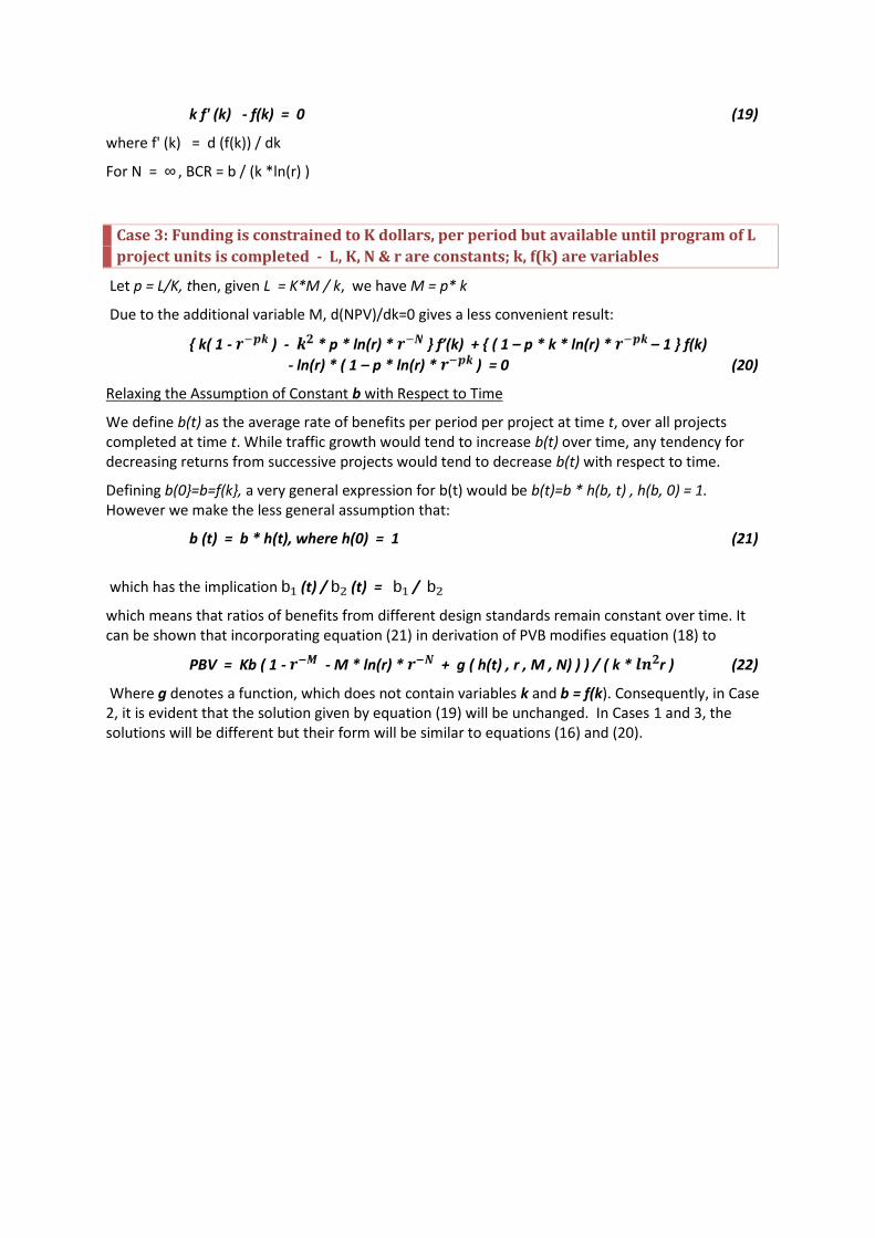
k f' (k) - f(k) = 0 (19)

where f' (k) = d (f(k)) / dk

For N = ∞, BCR = b / (k *ln(r) )

Case 3: Funding is constrained to K dollars, per period but available until program of Lproject units is completed - L, K, N & r are constants; k, f(k) are variables

Let p = L/K, then, given L = K*M / k, we have M = p* k

Due to the additional variable M, d(NPV)/dk=0 gives a less convenient result:

{ k( 1 - ) - * p * ln(r) * } f’(k) + { ( 1 – p * k * ln(r) * – 1 } f(k)- ln(r) * ( 1 – p * ln(r) * ) = 0 (20)

Relaxing the Assumption of Constant b with Respect to Time

We define b(t) as the average rate of benefits per period per project at time t, over all projectscompleted at time t. While traffic growth would tend to increase b(t) over time, any tendency fordecreasing returns from successive projects would tend to decrease b(t) with respect to time.

Defining b(0}=b=f(k}, a very general expression for b(t) would be b(t)=b * h(b, t) , h(b, 0) = 1.However we make the less general assumption that:

b (t) = b * h(t), where h(0) = 1 (21)

which has the implication b (t) / b (t) = b / bwhich means that ratios of benefits from different design standards remain constant over time. Itcan be shown that incorporating equation (21) in derivation of PVB modifies equation (18) to

PBV = Kb ( 1 - - M * ln(r) * + g ( h(t) , r , M , N) ) ) / ( k * r ) (22)

Where g denotes a function, which does not contain variables k and b = f(k). Consequently, in Case2, it is evident that the solution given by equation (19) will be unchanged. In Cases 1 and 3, thesolutions will be different but their form will be similar to equations (16) and (20).

Appendix D: Decision for Mutually Exclusive Projects with & Without Budget Constraints

Graphical Derivation of Results

In Figures 16 and 17, OA, OB, OC, OD represent four mutually exclusive projects with PVCs and PVBsas shown in Figure 16 and NPVs as shown in Figure 17.

However, the choice between these four mutually exclusive projects is equivalent to the choicebetween four dependent projects OA, AB, BC and CD. The dependency is obvious. In the givensequence, any one project is dependent on all those preceding it.

Unconstrained Budget

We apply the decision context type (i) rules for BCR and NPV from Table 1 to the dependent projectsin the given sequence starting with OA. We find that OA, AB and BC satisfy the respective rules ( BCR≥ 1 ) and ( NPV ≥ 0 ), but CD does not. Selecting OA+AB+BC is equivalent to choosing OC. Theappropriate decision rules can be inferred from Figures 16 and 17 and they are:

choose project that maximises NPV (Figure 17)

choose project that has least MBCR ≥ 1, (Figure 16)

choose project that has least MNPV ≥ O, (Figure 17)

Constrained Budget with Shadow Price

We apply decision context type (ii) rules ( BCR ≥ λ) and ( NPV ≥ (λ − 1 ) *K ) to the dependentprojects in sequence. These rules mean: accept a project if its slope (e.g., that of line OA) ≥ λ, inFigure 16 or (λ − 1), in Figure 17. We find that OA and AB satisfy the rules and BC does not. Thecorresponding best mutually exclusive alternative is OB, and from Figures 16 and 17 we infer thedecision rules contained in Table 1 for this context:

choose project that maximises NPV − − ∗ , (Figure 17)

choose project that has least MBCR ≥ , (Figure 16)

choose project that has least MNPV ≥ ( − ) * ( , ) , (Figure 17)

Figure 16: PVB versus PVC for Mutually Exclusive Projects OA, OB, OC & OD

Figure 17: NPV versus PVC for OA, OB, OC & OD

REFERENCES

Australia (1966), Treasury Information Bulletin, Investment Analysis Supplement, Canberra, July.

Australia (1976), Consolidated set of design standards for national highways in Australia.

Bayley (1979), NIMPAC Road Planning Model, NAASRA Secretariat, Sydney.

Berry, D.J. (1979), Developing strategies for rural road improvements. Proc. NZ Roading Symposium.

Berry, D.J. and Both, G.J. (1980), Stage Development of traffic capacity improvements to major ruralroads in Victoria. Workshop on the Economics of Road Design Standards, Bureau of TransportEconomics, Canberra.

Both, G.J. (1978), Determining road priorities at a state wide level. Proc. 2nd Conference, RoadEngineering Association of Asia and Australasia, Manila, October.

Both, G.J. and Bayley, C. (1976), Evaluation procedures for rural road and structure projects. Proc.8th ARRB Conference: Transport Planning and Economics, vol. 8, part 6, 6-25.

Bowyer, D.P. (1976), Mathematical programming as an aid in road project programming. Proc. 8thARRB Conference: Transport Planning and Economics, vol. 8, part 6, 26-33.

Buckley, D.J. and Gooneratne, S.G. (1974), Optimal scheduling of transport improvements to caterfor growing traffic congestion, Journal of Transport Economics and Policy VIII, 2.

Cassidy, P.A. and Gates, R.C. (1977), Simulation, Uncertainty and Public Investment Analysis, NorthBrisbane College of Advanced Education Press.

Chansky, S.B. (1975), Must highway reconstruction always comply with design standards? TrafficEngineering, July, 58-59.

Dart, O.K. and Mann, L. (1970), Rural highway geometric relationships to accident rates in Louisiana,Highway Research Record No. 312, 1-16.

Dasgupta, A.K. and Pearce, D.W. (1978), Cost-Benefit Analysis: Theory and Practice, Macmillan,London.

de Neufville, R. and Mori, Y. (1970), Optimal highway staging by dynamic programming,Transportation Engineering Journal, Proc. ASCE 96, 11-24.

de Neufville, R. and Stafford, J.H. (1971), Systems Analysis for Engineers and Managers, McGraw-Hill,New York.

Department of Construction (1976), Hume Circle Improvement, Report Prepared for the NCDC,August.

Feldstein, M.F. (1964), Net Social Benefit Calculation and the Public Investment Decision, OxfordEconomic Papers, March, 114-131.

Fisher, N.W.F. et al (1970), The application and development of the rural roads evaluation modelMERRI, Proc. Fifth ARRB Conf, 5, 1, 187-220.

Forbes, C.E. and Womack, R.R. (1976), A new direction £or the highway program, in TransportationResearch Board, Transportation programming and management, Transportation Research Record585, Washington, DC.

Gould, J.R. (1972), On investment criteria for mutually exclusive Projects, Economica, 39, 153, 70-77.

Hirschleifer, J. et al (1960), Water Supply, Chicago.

Howell, D.T. (1977a), Selection of design flood, in A. Patterson ed. , Australian rainfall and runoff:Flood analysis and design, Inst. Eng. Aust., Canberra.

Howell, D.T. (1977b), Design flood determination: A simple decision problem? Hydrology Symposium1977, Inst. Eng. Aust. , 114-118.

Howell, D.T. (1980), Multiple objective criteria for selection of hydrology standards for road projectsin different terrain types. Workshop on the Economics of Road Design Standards, Bureau ofTransport Economics, Canberra.

Hutchinson, B.G. (1972a), Economic criterion for highway capacity determination, TransportationEngineering Journal, August, 465- 475.

Hutchinson, B.G. (1972b), Programming of regional highway investments , TransportationEngineering Journal, August, 493-502.

Institution of Engineers, Australia (1977), Australian Rainfall and Run off: Flood analysis and design.

Jorgensen Associates (1975), Methods for evaluating highway safety improvements, NCHRP Report162, Transportation Research Board, Washington, DC.

Jorgensen Associates (1978), Cost and safety effectiveness of highway design elements, NCHRPReport 197, Transportation Research Board, Washington, DC.

Kaesehagen, R.L. (1977), Discussion paper by Advance Planning Engineer, Seminar on DesignStandards, Main Roads Department , Perth, WA.

Krosch, A.D. (1980), Experiences with NIMPAC and implications of alternative standards for ruralhighways in Queensland. Workshop on the Economics of Road Design Standards, Bureau ofTransport Economics, Canberra.

Latham, J. (1980), Staging Provisions for National Highway Standards, Workshop on the Economics ofRoad Design Standards, Bureau of Transport Economics, Canberra.

Lind, G. (1976), Selection of cross-section under consideration of the shortage of financial resources,Proc. OECD Symposium on Methods for Determining Geometric Road Design Standards, Denmark.

McLean, J.R. (1978), The role of geometric standards. Proc. 2nd Conference Road EngineeringAssociation of Asia and Australasia, vol. 2, October, 65-75.

McLean, J.R. (1976), Economic implications of road design standards, Internal Report AIR 000-29,Australian Road Research Board, Melbourne.

Mishan, E.J. (1971), Cost-Benefit Analysis, George Allen and Unwin, London.

NAASRA (1976), Policy for Geometric Design of Rural Roads, National Association of Australian StateRoad Authorities, Sydney.

NAASRA (1979), Guide to the design of rural roads: Revision of 'Policy for Geometric Design of RuralRoads', Final Draft, August.

National Highway Study Team (1973), Final Report, Department of Transport, Australia.

Pierson, G. and Bird, R. (1976), Business Finance, second edition, McGraw-Hill, Sydney.

Pouliquen, L.Y. (1970), Risk Analysis in Project Appraisal, World Bank Staff Occ. Papers No. 11, IBRD,US.

Rahmann, W.M. (1976), Program allocation by simulation - an alternative to cost-benefit analysis.Proc. 8th ARRB Conference: Transport - Planning and Economics, vol. 8, part 6, 1-5.

Read, N.S.L. (1971), The effects of gradient on highway cost. Proc. NZ Roading Symposium, 284-296.

Reutlinger, S. (1970), Techniques for Project Appraisal Under Uncertainty, World Bank Staff Occ.Papers, No. 10, IBRD, US.

Taplin, J.H.E. (1980), An economist's view of the multiple objectives of government in road fundingand the setting of design standards. Workshop on the Economics of Road Design Standards, Bureauof Transport Economics, Canberra.

Trilling, D.R. (1978), A cost effectiveness evaluation of highway safety countermeasures, TrafficQuarterly XXXII, 1, 41-66.

Vroombout, F. (1980), Practical considerations for flood design standards for bridges and culverts.Workshop on the Economics of Road Design Standards, Bureau of Transport Economics, Canberra.