1  

American Incomes 1774-1860*

Peter H. Lindert (University of California – Davis)

Jeffrey G. Williamson (Harvard University and the University of Wisconsin)

Abstract

Building what we call social tables, this paper quantifies the level and inequality of American incomes from 1774 to 1860. In 1774 the American colonies had average incomes exceeding those of the Mother Country, even when slave households are included in the aggregate. Between 1774 and 1790, this income advantage over Britain was lost, due to the severe dislocation caused by the fight for Independence. Then between 1790 and 1860 US income per capita grew even faster than previous scholars have estimated. We also find that the South was initially much richer than the North on the eve of Revolution, but then suffered a severe reversal of fortune, so that by 1840 its white population was already poorer than free Northerners. In terms of inequality, our estimates suggest that American colonists had much more equal incomes than did households in England and Wales around 1774. Indeed, New England and the Middle Colonies appear to have been more egalitarian than anywhere else in the measureable world. Income inequality rose dramatically between 1774 and 1860, especially in the South. The paper offers an open-source style, since our data processing is posted on http://gpih.ucdavis.edu (click on the folder “American incomes 1774-1870”). Detailed defense of the 1774 and 1800 benchmarks can be found in our previous NBER working paper (17211, July 2011), although the estimates reported here are revised. The 1860 benchmark is completely new.

Key words: Inequality, growth, early America. JEL: N11, N31, O47, O51

Acknowledgements Our work has been aided greatly by a battalion of scholars and archivists. The list of helpful colleagues includes Jeremy Atack, Paul Clemens, Paul David, Farley Grubb, Herb Klein, Allan Kulikoff, Bob Margo, Paul Rhode, Josh Rosenbloom, Carole Shammas, Billy Gordon Smith, Richard Sylla, Sam Williamson, and especially Tom Weiss. Archival help was supplied by, among others, Jan Kinzer (Pennsylvania State Archives), Diana McCain (Connecticut Historical Society), Clifford C. Parker (Chester County Archives), and Marc Thomas (Maryland Historical Society). We thank them, yet absolve them from any responsibility for the results presented here. We also acknowledge with gratitude the research assistance of Lety Arroyo-Abad, Julianne Deitch, Sun Go, Patricia Levin, David Nystrom, Brock Smith, and especially Nick Zolas. The paper has also benefitted from earlier suggestions by participants at the University of Warwick – Venice, the University of Michigan, the Institute for Research on Poverty at UW-Madison, the NBER’s summer DAE workshop, and the World Economic History Congress at Stellenbosch.

      2  

I. Growth and Inequality Debates about America’s First Century

Economic historians need fresh information about American income levels and their

distribution at the end of the colonial era and the dawn of independence in order to understand

growth and evolving social structure over America’s first century. The need for more evidence

becomes apparent whenever we try to cast back from the late colonial period, to project ahead

from the colonial and early federalist years, or to view American incomes in trans-Atlantic

perspective.

Modern debate over American growth experience before 1840 starts with Paul David’s

classic 1967 article offering what he called controlled conjectures. David (1967, 1996), Robert

Gallman (1992, 1999), Thomas Weiss (1992, 1993a, 1993b, 1994), and others focused their

conjectures on the division of the economy into large output sectors, each with its own labor

force and labor productivity growth. All of these competing estimates have been built up from

the output side in the spirit of Simon Kuznets. This paper offers something quite different,

building up estimates from the income side in the form of what have been called social tables.

Not only does our approach offer fresh new estimates of American incomes at three benchmark

dates – 1774, 1800, and 1860 – but it also allows us to estimate income distribution within

regions and for America as a whole. Until recently, our social tables approach would have been

impossible given a paucity of data on the occupations and the sector mix of the labor force

before 1840. The early censuses did not help much with these, except to give indicators that

should have affected labor force participation, such as sex, race, age, region, and urban/rural.

Accordingly, we have long thought that a new attack on the issue of early American growth

must feature new information on the American labor force by occupation in the form of social

tables. Even though many household heads were simply called artisans, merchants, farmers,

planters, farm hands, or slaves, it helps considerably to know what labor force shares they

represented, where they lived, their average incomes, and how those incomes changed over

time.

Our interest in American incomes around the time of the Revolution is enhanced by

viewing them from across the Atlantic. Angus Maddison (2007) estimated that it was not until

after the 1870s that the United States caught up with the United Kingdom in real GDP per

capita, though active debate has ensued about the uncertainties of his index numbers.

      3  

Maddison’s estimates need to be reconciled with the fact that America attracted a significant net

emigration from the Mother Country and that colonial and republican population growth was

much faster there. In the light of current research on the Great Divergence, on the history of

European incomes, and on the continued use of the Maddison world income estimates, we think

the time is ripe to add data from the American side to compare with the new estimates for

Europe.

We can now offer new estimates based on more archival data than were available to

earlier researchers. The estimates are offered as an “open-source” presentation of our detailed

data and procedures on the internet, for both negative and positive reasons. The negative reason

is that many scholars might resist accepting some new estimates based on vulnerable primary

data, wishing to offer their own estimates. The positive reason for open sourcing is the

dynamism of the database itself. The information explosion that has offered us new data will

continue to offer additional data to all scholars in the future. Maximizing the disclosure of our

data and procedures accelerates the opportunities for improving the reliability of the estimates.

Hence, our work is inextricably tied to a growing downloadable set of spreadsheet and text files

at http://gpih.ucdavis.edu.

Our findings confirm some conventional wisdom about American growth and inequality

between 1774 and 1860, yet contradict others, and also introduce some brand new issues. They

certainly offer a much clearer view of colonial American inequality and how the incomes of

different classes compared with those of their counterparts in England. Inequality was much

lower in 1774 and 1800, especially among free whites, than in England. Inequality was also

lower than in the United States today. We find higher colonial incomes in 1774 than have

previous scholars, especially higher in the Southern colonies. Indeed, average incomes in 1774

were higher than those in England and Wales, using either exchange rates or purchasing power

parity guesses. But they may have been lower in 1800. Thus, America gave up its per capita

income leadership to England between 1774 and 1800, as a price paid for independence. Our

estimates raise new questions about what happened between 1774 and 1800, during the

disastrous war years and the costly post-war struggle with confederation, only partially offset by

the 1790s boom. But our findings also suggest that America’s growth rate between 1800 and

1860 was quite a bit faster than has been previously thought. The Old South did not share that

      4  

dynamic experience, however, since its reversal of fortune,1 which had started after 1774,

continued after 1800.

II. Estimating Three Social Tables for America’s First Century: 1774, 1800, and 1860

A. The 1774 Colonial Evidence

Our approach starts by counting people by occupations or social classes, and mustering

evidence about their average incomes. That is, we build national income and product accounts

(NIPA) from the income side. This departs from all recent scholarship on early American

growth, which has built its real income series from the production side, and then used price

indexes to report nominal incomes for the price levels of that time. Historians will immediately

recognize our approach as that of building social tables, in the “political arithmetick” tradition

spawned by such Englishmen as Sir William Petty and Gregory King in the 17th century. That

is indeed our approach here, as it has been in other publications of ours.2 In fact, at least two

early American efforts tried to imitate Petty with their own calculations of what their region was

worth – presumably to guess at its ability to pay taxes and fight wars.3

Fortunately, the archives continue to accumulate early local returns that recorded

people’s occupations, including such social labels as “Esquire” or “widow” in the English

tradition. Reconstructing society from these sources is no easy task, however, and will continue

to be challenging as the primary data accumulate in the future. This challenge requires that the

reader take a tour of our data warehouse in which we counted colonials and determined their

incomes. The tour will be shorter than the longer one offered in our earlier working paper

(Lindert and Williamson 2011: section II)).

Any social profile of Americans on the eve of the Revolution must start from local

censuses, supplemented by tax lists and occupational directories, and supported indirectly by the

earliest national censuses of 1790 and 1800. Fortunately, the recent electronic revolution has

made local enumerations from the late 18th century much more accessible. While all records

before 1790 were local, aggregate regional counts can be developed by assuming that

proportions from one documented locality represents those of other localities in the same region

and with the same population density, urbanization levels, and qualitative attributes.

      5  

Our estimates of early American work status, location, and living arrangement start from

basic population counts themselves, and then add early labor force estimates (themselves

constructed from labor participation rates by age-sex-slave/free cells), before dividing up that

labor force by occupation and by household headship status.

Population census counts. The few local censuses from the colonial period are now

collated and referenced in the colonial section of Historical Statistics of the United States, both

in the Bicentennial Edition (1976) and in the Millennial Edition (2006). These offer detail by

sex, race, free/slave status, and rough age distributions for seven colonies; we clone the other

six colonies from the seven, matching contiguous colonies.

Labor force participation rates. Next we derived the numbers of persons in the labor

force for each demographic group defined by place, sex, race, free/slave, and age. The

conventionally defined labor force consists of all persons generating product sold in significant

part (or, for slaves, demanded in significant part) outside the household.

To convert population into labor force, we use the detailed labor participation rates for

1800 supplied by Thomas Weiss. It seems reasonable to assume that there were no behavioral

changes in the rates defined in the detailed cell-specific Weiss estimates, which give separate

rates for such cell categories as urban Pennsylvania’s free white females age 10-15, or rural

South Carolina’s male slaves over the age of 10, or small town Connecticut’s free white males

aged 16 and older. However, since these categories changed in relative importance over time,

the regional and national labor participation rates could and did change between 1774 and 1800.

Recorded occupations. Sketching the social make-up of the labor force requires detailed

occupation counts for different localities. We draw on newly accessible counts for years near

1774, though only for a few places, only for parts of the labor force, and only with the help of

some comparison of occupational mixes over time and space.

Our effort to reconstruct the American social structure on the eve of the Revolution uses

local tax assessment lists and occupational directories. Such lists allow us to create the

following occupational groups for the free population: officials, titled, and professionals; big

city merchants and shopkeepers; small town and rural merchants and shopkeepers; skilled

artisans in manufacturing; skilled in the building trades; farmers (renters, sharecroppers and

owner-operators); male menial laborers; and female menial laborers. Our new data re-shape the

standard view of the colonial occupational structure. For example, relative to Alice Hanson

      6  

Jones (1977), our estimates shift a lot of the Middle Colonies’ labor force from middling

farmers to less wealthy craftsmen and laborers, and to males with no stated occupation.

For the urban South, we use the 1790 directory for Charleston but scaled back to

conform to the estimated total population of Charleston in 1774. One gets the same

occupational patterns by starting with Alice Hanson Jones’s w weights for a sample drawn from

four Southern states. In either case, one must adjust for the over-representation of landowners

and, especially, slaveholders (both absent from their plantations). We adjust the Jones weights,

guided by some very useful local censuses from three North Carolina counties in 1779-1782.

These enumerated all household heads according to whether they held slaves or real estate or

both or neither. We assume that the same adjustment of weights is required in Charleston as in

the rest of the South.

For the rural South, we carried out the same adjustment away from slaveholders and

landowners, giving instead more weight to ordinary farmers. One could wish for a broader

sampling of the rural South than just the Alice Hanson Jones sampling from four states, plus our

new sampling from the three North Carolina counties. There are other rural Southern county

assessment documents on the internet, but only very few are for dates earlier than 1798, and

none of the lists we have seen record the occupations of the household head.

Unrecorded occupations. Persons with occupations recorded by tax assessment lists or

urban occupational directories fall short of the persons in the labor force. In most cases the lists

even fail to capture all household heads, the exception being those three counties of rural North

Carolina between 1779 and 1782, which seem to have captured all free household heads.

Not all members of the 1774 labor force without recorded occupations are equal. Some

lack an occupational label despite assessed wealth. Some lack an occupational label, and are

listed as tax-exempt because they had zero or near-zero wealth. We distinguish three groups

whose occupations aren’t recorded: free males with positive wealth listed but without a

recorded occupation; free females with positive wealth listed but without a recorded occupation;

and free persons listed without a recorded occupation and having zero or near-zero wealth.

Counting Households. One could avoid measuring household headship if we were

interested only in measuring aggregate national product, since it depends only on who is in the

labor force and their average income. Yet we need the headship rates by occupation to measure

inequality.

      7  

Households are the income recipient units used here to measure income inequality, for

both practical and theoretical reasons. Previous investigators have been forced to confront the

simple fact that taxable property, such as real estate, is used by all household members, even if

only one is the owner and taxpayer. The prevailing practice is to measure income inequality

among households, not among individual income earners. In order to compare apples with

apples, we do the same. That is the practical reason. The theory comes from Simon Kuznets

(1976), who emphasized the superiority of the household focus. Caring about economic

inequality means caring about how unequally people consume resources over their lifetimes.

Even if data constraints force us to study annual inequality rather than life-cycle inequality,

Kuznets argued that annual income per household was a better measure of income distribution

than one using income per earner.

Since the early population censuses usually did not count households, some assumptions

must be invoked to decide who were household heads and who lived under the same roof with

the head. Fortunately, historians of early America have already grappled with this issue.

Following the leads of Billy Gordon Smith (1981, 1984, 1990) and Lucy Simler (1990, 2007;

Clemens and Simler 1988) in particular, we estimate the number of household heads from

c1774 and c1800 population data from invoking assumptions detailed elsewhere (Lindert and

Williamson 2011: Section II). These assumptions have generated total households by place –

that is, by region and by urban versus rural.

By subtraction, we derive the number of household heads that are missed by the listed

occupation accounts. The shares of heads omitted are often large when the occupational data

come from the tax lists and the urban directories. The colonial business directories and the tax

lists missed more than 30 percent of all households. Left uncorrected, such counts would

underestimate total income and bias inequality downwards, since many of the unregistered were

poor. Fortunately, the tax lists nearer 1800 seem to have captured something like the full

population, at least according to our samplings from New York State property tax rolls that

began around 1799. The same should have been true of the federal direct tax of 1798, which

required a household enumeration subject to external audit.

Which groups were most frequently omitted in the colonial era? The literature has

advanced the plausible intuition that the omitted consisted mainly of the tax-excused poor,

whose names could be safely omitted from tax lists or business directories. Yet, there is also

      8  

some evidence that many in the middling and rich groups may also have been omitted, or at

least that their wealth was under-assessed. Three questions need to be answered dealing with

those who were in the labor force (LF), according to the censuses and the Weiss estimates of

labor force participation rates, yet who were not reported as household heads (HHs): First, how

many of them were there for each place defined by region and by urban/rural? Second, what

kinds of occupations did they have? Third, whose households did they live in? Guided by the

censuses, we identify the following groups in the labor force who were not household heads:

free white males and females, ages 10-15; free white males and females, ages 16-up, but not

household heads; free black males and females, ages10-15; free black males ages 16-up, minus

free black household heads; free black females ages 16-up; white indentured servants in

Maryland, the only colony that labeled them separately in a census near 1774; and slaves ages

10-up. Some of these contained laborers who were almost surely paid only unskilled wages,

while others were spread over occupations of higher earnings. What we assumed about their

occupational distribution, and thus their incomes, is reported elsewhere (Lindert and

Williamson 2011: Section II).

For inequality purposes, and following Kuznets, we must also decide in whose

households these non-HH head members of the labor force lived. The data are almost non-

existent on this issue. We make the following assumptions about the non-head earners

“imported” into the households of others: For each region and urban/rural location (e.g. New

England big cities or rural South), the non-heads and their individual earnings are absorbed into

the same region and place. In other words, earners do not engage in long-distance commuting

between regions or between countryside and city. For the free population, we assume that the

average earnings of each non-HH head imported into free families is the same for all free

persons of that occupation in that place. Slave non-heads are taken into slave households only,

leaving household income the same as the retained earnings of all slaves. This same assumption

holds for the separately recorded group of Maryland servants, though the assumption is

redundant here because these are one-person households. These assumptions certainly can be

challenged. We emphasize one point about data sources: For each place defined by region and

by urban/rural, the aggregate imports of non-HH heads are driven by the census, the labor

participation rates, and by the household headship rates. But the allocation of non-HH heads to

      9  

households by place is not yet derived from micro-studies about how households shared

earnings, because few such studies exist.

Labor earnings by occupation, circa 1774. We are able to assign annual incomes to the

most ubiquitous occupations in each location, thanks to the enormous archival gleanings of

Jackson Turner Main’s The Social Structure of Revolutionary America (1965), Stanley

Lebergott’s Manpower in Economic Growth (1964), the work of Carroll Wright (1885), the

BLS (1929), T. M. Adams (1944), Winnifred Rothenberg (1985), several articles of Donald

Adams (1968, 1970, 1982, 1986, 1992), and the contributions of a few others. Their time-

consuming collection of newspaper quotes and account book entries must be used with care.

Some are in the depreciated local colonial currency, whereas others are in (British) pounds

sterling. Fortunately, most sources, and Main in particular, are careful to say which was which.

Finally, we assume that slave and free labor marginal product was the same for all occupations

where they both worked, but, of course, the slave only retained or consumed a fraction of that

marginal product.4

Some of the earnings are annual, as for white collar professionals and farmers, but many

are monthly, weekly, or daily rates of pay, requiring assumptions about how many days or

months they spent in gainful employment each year. We believe that for those days or months

in which a colonist did not hold his or her main stated job, he or she nonetheless filled in with

other productive work, like weaving and farming at home, and some of this output was traded

on the market. Thus, our “full-time” estimates assume that daily or monthly full-time

equivalent (FTE) workers performed productive work of some kind for 313 days a year

(excluding only Sundays). This assumption implies, of course, that we include more non-market

work in our income estimates than do other scholars that include only or mainly market work in

their output estimates. However, to imitate the labor force behavior that other scholars may have

assumed in estimating early American GDP, and as sensitivity analysis, we also calculate “part-

time” estimates that use fewer labor days per year.5

We enlarged the concept of labor earnings to include farm operators’ profits, estimated

by Main, plus slaves’ and indentured servants’ retained share of what they earned (discussed

above). As we noted previously, this labor income amalgam we have called “own-labor

incomes”.

      10  

Property income in 1774. Our property income estimates benefit from Alice Hanson

Jones’s exhaustive and masterly study of America’s wealth structure in 1774, based on her 919

probate inventories and supporting documents.6 A key advantage of her data is that they

identify the occupation or social status of most of the people in her colonial sample. We have

examined her data and procedures in great detail, and find no flaws.7 Jones realized that a

probate-based sample ran the risk of overstating average wealth, and understating wealth

inequality, because probate was more likely for the deceased rich than poor. She went to

enormous lengths to adjust for this, ending with what she called w*B estimates that were meant

to capture more of the poor. We have moved in the same direction, using a different procedure.

Our greater weighting of the poorer households was achieved by introducing the new data on

occupational structure described. As it turns out, our estimates imply an even greater probate-

wealth markdown than did her w*B estimates.

Wealth is not property income or total income. Jones confined her income-measurement

efforts to brief conjectures about wealth-income ratios, using aggregate capital-output ratios

found in the macroeconomics literature of the 1970s.8 We have followed a different route, in

order to exploit the wage data just described. Our reading of the limited evidence on colonial

rates of return suggests that, on average, assets probably earned a net rate of return of about 6

percent per annum.9 Later we will quantify the sensitivity of our aggregate income estimates to

this 6 percent rate of return.

The gross rate of return, which is more appropriate to the calculation of gross national

product for comparison with other studies, equals this net 6 percent plus rates of depreciation

that differed by asset. Following NIPA accounting standards, we have assumed zero

depreciation on financial assets and real estate (positive depreciation offset by rapid capital

gains), 5 percent for servants and slaves, 10 percent for livestock and business equipment, and

zero for net changes in producers’ perishables and crops.10

Combining own-labor income and property incomes. Here we reap big returns to having

invested so much effort in gathering occupation data. Since own-labor incomes and property

incomes are both arranged by occupation, we can combine the two to get their total incomes, by

region, by urban/rural, and by socio-economic group.

Households were practically the whole economy. Our calculations offer what NIPA

accountants call total private income of the household sector. The colonial government sector’s

      11  

contribution consisted only of the wages and salaries of government employees and military

personnel (already included in our occupations and own-labor earnings). There were no

government corporations in 1774. Nor do we need to worry about the retained earnings of

private corporations, since there were so few of them by the end of the century. The same

assumptions will be made for 1800. The non-household sector will take a larger share of

national income for 1860, however.

B. The 1798-1800 Early Federalist Evidence

Our next benchmark for appraising national income is the census year 1800. On the labor-

income side, our procedures for 1800 are roughly the same as those we applied to 1774, though the

data sources are more copious and of higher quality. What is distinctive about the estimates for 1798-

1800 relates not to labor incomes but to property incomes. To fund a possible conflict with France,

Congress passed the first direct tax, a one-off tax levied on real estate wealth and on the numbers of

slaves.11

The 1798 direct tax returns remain the most useful source available for the property income

side of 1800 national income estimation. True, one might view these returns with some suspicion: Can

we trust the quality of the data extracted by tax collectors from a new nation that had just shed its royal

government partly over tax issues? Such suspicion is indeed warranted, especially given some

evidence that properties had already been under-assessed in tax returns of the previous two decades.12

The 1798 direct tax under-assessed market values by something like 15.5 percent in New England and

the Middle Colonies, a figure based on a contemporary study of marketed real estate in Connecticut in

that same year.13 We have adjusted upwards our 1800 property income estimates for this 15.5 percent

underassessment in New England and the Middle Colonies, and also for the 7 percent rise in average

asset values from 1798 to 1800 suggested by the contemporary Samuel Blodget (1806).

The South might have under-assessed rich households’ realty, and slaves, by even more than

the North. We have three clues about the degree of underassessment there. Two of these relate to

slaves and do not affect our income estimates. The third relates to real estate, and it does affect our

income estimates.

The first clue arises from slave counts. The tax return of 1798 reported only 86,840 slaves of

taxable age 12-50 and 323,905 slaves overall. These numbers are much too low and also imply an

      12  

implausibly low working-age share for the slave population (0.268). Indeed, only two years later the

1800 census reported 513,905 slaves aged 10-up and 835,490 slaves overall. Even the 1790 census

reported far more slaves than were revealed in the 1798 tax returns. Fortunately, we were able to

reject the 1798 tax-return slave counts in favor of the 1800 census, combined with the Fogel-

Engerman (1976, updated 2006) sample values for the rental incomes derived by slaveholders.14

A second clue supporting underassessment in the South lies with the overall tax valuation of

slaves, rather than just their numbers. According to Timothy Pitkin’s (1817) summary of the 1798

returns, slave taxes were only 21 percent of all reported realty plus slave taxes in the South Atlantic,

while in 1774 slave values were 58.1 percent of all slave plus realty value in that region. Either the

market value of slaves relative to the value of real estate dropped spectacularly over the quarter

century, or slaveholders gained a considerable tax break relative to real estate owners. It seems clear

that the fifty-cent tax per slave aged 12-50 years was based on an undercount of those slaves.15

Fortunately, our estimates of slaveholder incomes are based on the market value of slaves rather than

on the tax assessor’s slave values, and our slave counts are based on the 1800 census.

In contrast with the first two clues, the third underassessment clue does have implications for

our southern property income estimates. The South Atlantic (here excluding Delaware) paid 38.1

percent of the eastern US realty tax in 1798. This share was tied by law to the South Atlantic share of

the free population of the eastern states in 1800 (35 percent). Note that the region’s 38.1 percent tax

share is much lower than the 57.7 percent share of the thirteen colonies’ real estate wealth in the

probate valuations for 1774.

There are two possible explanations for the discrepancy. The first possibility is that the South

could have under-assessed its 57.7 percent share of the market-based value of all realty in the 13

colonies, reporting only 38.1 percent. This implies that we should mark up greatly South Atlantic real

estate values in 1798-1800, from a South/North assessment ratio of 38.1/61.9 = 0.62 to a market ratio

of 57.7/42.3 = 1.36.16 We will call this assessment our upper bound assumption. The second

possibility is that Southern realty was truly worth only 38.1 percent of total market value, implying

that its relative real estate values must have crashed in the Revolutionary war and postwar years. This

assessment will be called our lower bound assumption.

Neither assumption seems persuasive. The lower bound assumption would disregard the three

clues implying that the South got away with a lower assessment rate. The upper bound assumption

suggests something that would have been spotted by Northern members of Congress, and we would

      13  

have read their outcry. Its implication that the South Atlantic suffered relative war and postwar losses

that enormous also strains belief. The true underassessment differential probably lies between these

two extremes. We therefore settle on the middle ground: that is, we assume that the North had the 15.5

percent underassessment of real estate demonstrated in the 1798 Connecticut market study, and that

the South had the same 15.5 percent underassessment plus half of the upper bound extra

underassessment. Thus, the adjustment for the extra Southern underassessment raises real estate plus

slave wealth values by 30.1 percent for the South Atlantic. This combined with the nationwide

underassessment of real estate by 15.5 percent raises real estate plus slave wealth values by 40.4

percent for the South Atlantic, or 27.7 percent for the whole Eastern seaboard.

Since the 1798 returns covered only real estate and slaves, we had to use the same ratios of

total property/(realty plus slave values) obtained from the 1774 evidence to inflate them to total

property. We apply region-specific ratios to each of the three colonial regions.

There is one other important difference between the data sources on the property side between

1774 and 1798-1800. The 1798 tax returns are very handy in that they were aggregated for us at the

time. But a serious drawback of the 1798 returns is that it reports no data on occupation. This means

that we cannot document the occupational distribution of total income for 1800, although we can

document the distribution of own-labor incomes and property incomes separately, as well as the

aggregate value of total income.

B. The 1860 Income Estimates: IPUMS Meets Wage History

The procedures for building social tables for each region in 1860 are essentially the same as for

1774. Once we again we have a fairly reliable source of data on wealth. Parallel to Alice Hanson

Jones’s wealth estimates, we now have the IPUMS random (“flat”) sample of households in the 1860

census. Again, we convert the wealth data into property incomes using a rate of return. To the real

estate wealth we applied a net rate of return of five percent, based on interest rates of that era. For

gross rates of return on other assets, we had to reckon the approximate share of “personal estate” that

tended to be slaves versus other productive assets and consumer assets. Drawing on the wealth

portfolio assumptions of Raymond Goldsmith for the US in 1850 and 1880, we came up with a gross

rate of return of 7.8 percent for the South and 7.3 percent for the non-South, the difference explained

by slaveholding, for which we used a depreciation rate of 11 percent.

      14  

Again, as with 1774, we were able to exploit the occupational detail to link property incomes

with own-labor incomes. The occupational weights are given directly in the IPUMS sample. For

1860 we have an even greater abundance of job-specific labor incomes, thanks to a variety of sources

– several authors’ gleanings from the Weeks and Aldrich Reports, Stanley Lebergott’s wage series,

Robert Margo’s rich data on civilian wage rates at Army Posts around the country, and the American

Almanac’s estimates of salaries for a wide variety of professional occupations. Slave retained

earnings were estimated from the Fogel-Engerman slave hire rates for 1858-1860, from free wage

rates, from the literature on the exploitation ratio for slaves, and from the IPUMS sample of slaves by

age, sex, and place. Finally, the pure residual profits of farm households were estimated from Lee

Craig’s sophisticated estimates for the North in 1860. For the South, we adjusted his profit estimates

in proportion to the wage rates of free farm laborers in different regions. For 1860 we continued to

apply our assumptions about the “part-time” work year for certain occupations.17

III. Income Levels and Growth: 1774-1860

The estimates speak to growth and inequality performance at the regional and national levels.

This section summarizes our findings about aggregate income levels and aggregate growth, while

Section IV reports inequality measures for our end-years 1774 and 1860.

A. The Income Level Estimates for 1774

The aggregate estimates of labor and property incomes shed new light on average income in

1774 and 1800, and the growth of income per capita over a quarter century of war, postwar, and

national emergence. The levels and composition of total personal income are shown in Tables 1-4, for

the three regions used by Alice Hanson Jones and for a geographically fixed “nation”, defined as the

13 colonies in 1774 and the easternmost 15 states plus the District of Columbia in 1800, and adding

states further west for 1860.

Here we stress two key results. First, the colonial South had an average income far above

those of New England or the Middle Colonies in 1774, even when one rightly counts slaves as

persons. That the South was so much richer in 1774 may not surprise those who have studied the

history of colonial wealth, but even average free labor earnings were higher in the South. (Wages were

not much higher occupation by occupation, but there were fewer unskilled free laborers in the South,

      15  

both farm and non-farm.) Second, these new estimates imply that real income per capita dropped

considerably over that quarter century. The 1774-1800 decline of about 20 percent looks almost as

serious in per capita terms as the 1929-1933 drop into the Great Depression. If other authors are

correct in reporting brisk income gains across the 1790s, then the Revolutionary disaster and

Confederation turmoil could have been America’s greatest income slump ever, in percentage terms.

Let us first scrutinize the levels of income at each date, before searching for explanations of the

implied net decline.

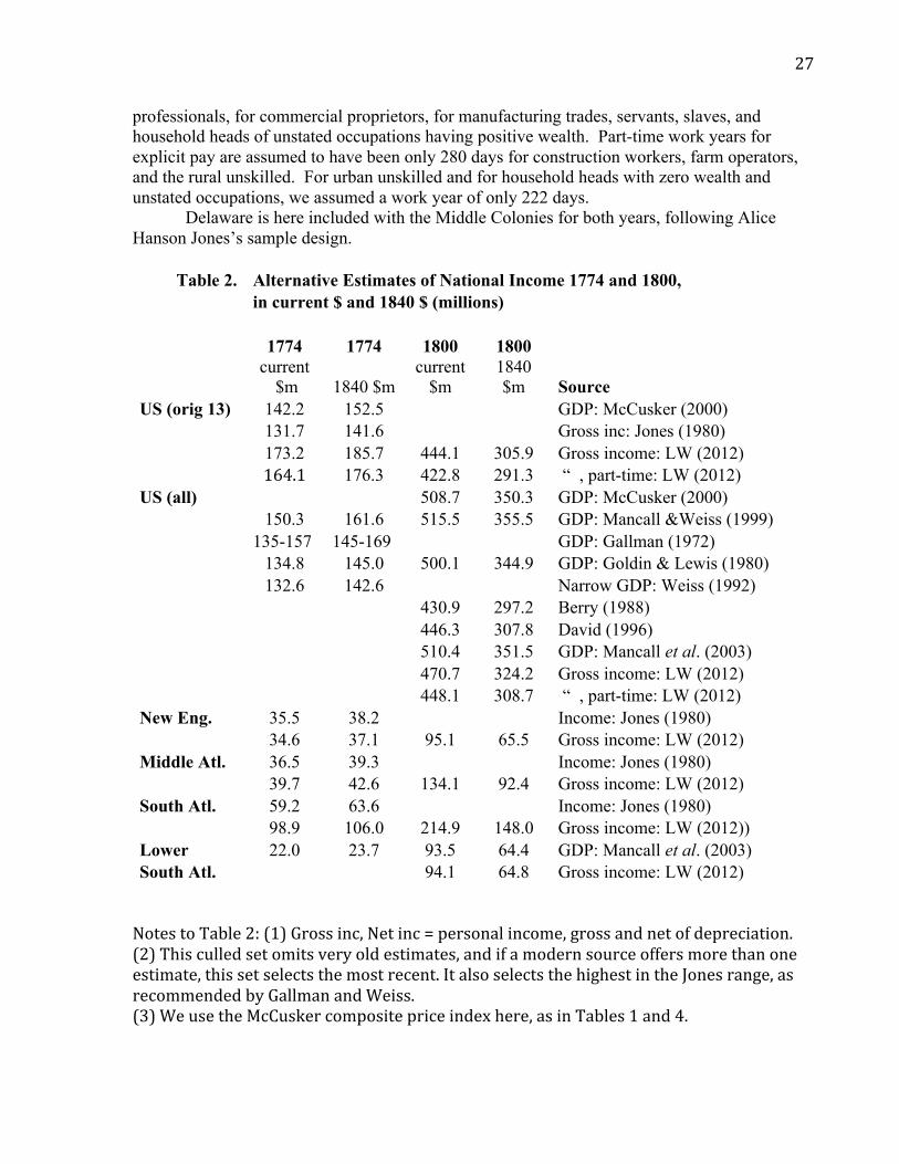
As Table 2 shows, our thirteen-colony estimate of 173.2 million dollars is 26 percent greater

than the average of the Jones and McCusker estimates (137.7 million), assuming a full-time work year

for all occupations, or 19 percent above Jones and McCusker if we assume that certain occupations

worked only part of the year. Yet our colonial income estimates differ greatly from those of Alice

Hanson Jones for only one region. There is little difference for New England, and for the Middle

Colonies we report incomes “only” about 9 percent higher than hers. The main source of the big

difference with Jones arises in the South, for which our income estimate ($98.9 million) is 67 percent

above that of Jones ($59.2 million).

For the 13 colonies as a whole, the large gap is not driven by any higher estimate of wealth per

household, since we rely on Alice Hanson Jones’ own work. Supplementing her data with our new

occupation weights, we get a slightly lower net worth per wealth holder than she did. Furthermore,

because we find many fewer households with wealth than her estimated number of “potential wealth

holders”, our aggregate wealth estimate is only about 70 percent of her implied total wealth.18

An alternative suspicion might be that our income estimates overestimate the net and gross

rates of return on productive wealth. It seems very unlikely that our 6 percent figure for 1774

overstates the net rate of return, the opportunity cost of not having lent at interest. The colonies and the

early republic had a legal usury limit of 6 percent that was vigorously supported by law and custom.19

That is, the usury constraint seems to have checked a strong demand for capital, so that the 6 percent

ceiling might very well have been below market. Could the (illegal, market) rate of interest foregone

by holders of directly productive assets have been higher, say 8 percent? We agree that this is a

distinct possibility, especially for 1800, for which the literature suggests even greater capital scarcity

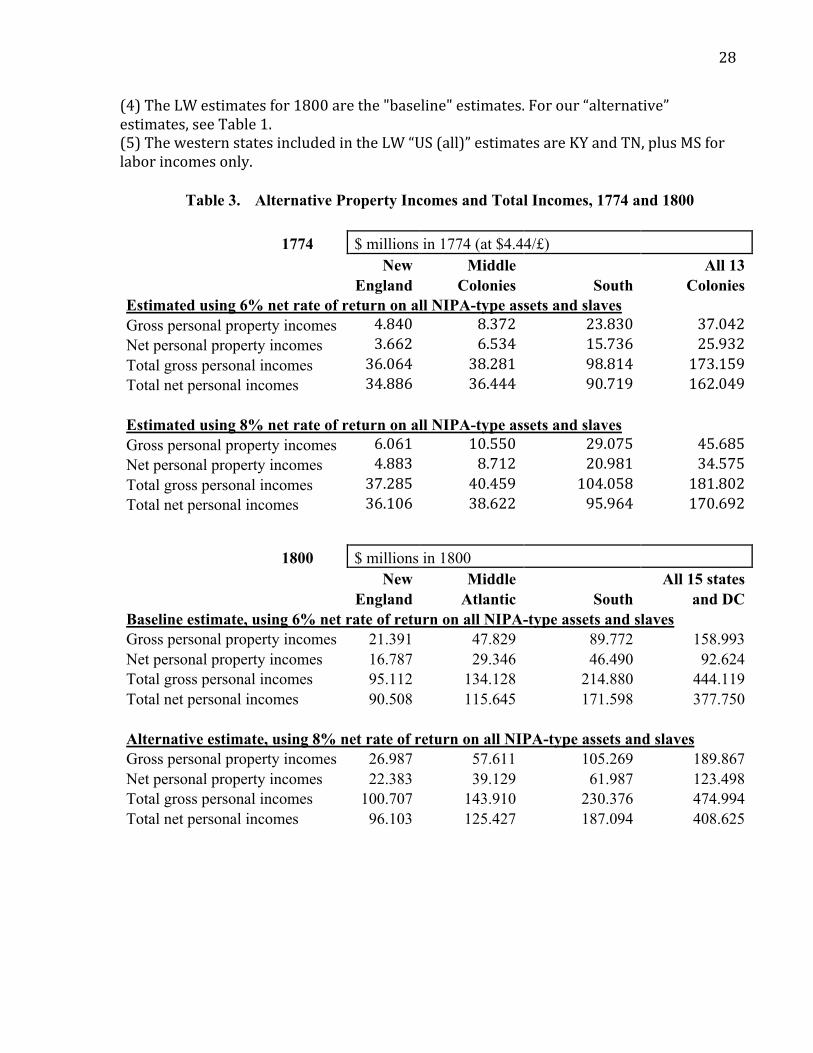
than for 1774.20 Table 3 shows the impact of assuming 8 rather than 6 percent. Shifting to the higher

rate of return would raise our total income estimates relative to those conjectured by other scholars.

      16  

So much for property income. What about our own-labor income estimates for 1774, supported

as they are by new occupation weights, full-time employment assumptions, and occupation-specific

wage rates? Could these have exaggerated labor income for the 13 colonies as a whole, thus raising

our aggregate income estimates above that of previous scholars?

What did Jones assume about rates of pay for labor, including the earnings retained by slaves?

In fact, she did not make any assumption at all, but took a single leap of faith that we have already

noted: By picking up some capital/output ratios quoted in the aggregate growth literature from the

1970s, she jumped from her impressive and reliable wealth estimates to less reliable total income

guesswork which stands or falls on her assumed aggregate wealth/income ratio (not necessarily the

same as a capital/output ratio). The macro literature offered Jones capital/output ratios ranging from

2.5 to 10 for the nineteenth and twentieth centuries. Within this wide range, she said, “I hazard that

ratios of three or three and a half to one may be reasonable”. Yet we find that the 1774 ratio of net

worth (wealth) to national income was only 1.89.21

The strikingly wide gap between Southern and Northern incomes in 1774 has a simpler

explanation. In 1774, unlike 1860 and later, the South had a very different mix of free men's

occupations, with a much higher propertied share and fewer poor. On the eve of the Revolution, the

South was still a frontier with high productivity in their exportable tobacco, rice, indigo, and cotton.

We find this contrast between the regional occupation mixes among free household heads in 1774:

among free household heads (%) New England Middle colonies Southern colonies Farm operators 43.9 25.8 72.7 Professions, commerce, crafts 11.0 32.5 14.3 No occupation given, some wealth 16.7 28.7 11.0 Menial laborers + those with zero wealth 28.4 13.0 1.9

Southern farmers not only had higher incomes than other farmers on the average, but they constituted

a larger share of households, while low-paying occupations took a lower share among free

Southerners. Therefore, the advantage of the colonial South should not seem surprising, even without

any gap in wage rates for given occupations.

B. The Income Level Estimates for 1800

Unlike those for 1774, our 1800 total income estimates are not above those offered by other

scholars. Rather, our estimates are in the middle of several competing estimates for the nation as a

      17  

whole (Table 2). Our 1800 estimates for the Lower South match those of Mancall, Rosenbloom, and

Weiss (2003), even though we used the income approach and they used the production approach. It

might seem comforting that our 1800 estimates are so close to others. However, ours would have been

a bit higher than most if we had been able to make all the adjustments that we feel are warranted. We

are especially concerned about two such adjustments.

The first potential adjustment is one already mentioned in connection with Table 5: using the

interest rate on public debt as a measure of the opportunity cost of assets, it appears that the net rate of

return on property was higher in 1800 than in 1774, presumably in response to Revolutionary War and

Confederation inflation, financial disruption, and perhaps even productivity advance.22 As we have

noted, if the interest rate tended to be 8 percent in 1800 versus 6 percent in 1774, then the 1774-1800

decline in real per capita income would be a bit less, using the “alternative” estimates for 1800 shown

in Table 3.

The second adjustment relates to an omission from the baseline 1800 estimates. We have no

1800 data documenting farm operators’ pure residual profits, as distinct from their asset returns or the

implicit value of their own physical labor. For 1774, we were able to use a few testimonies unearthed

by Main (1965) to guesstimate that the farm profit residual was 18.9 percent of all farm operators’

income in New England, 21.1 percent in the Middle Atlantic, 34 percent in the South, and 28.8 percent

for the 13 colonies as a whole. We cannot apply these ratios to 1800, however, since we lack any

delineation between farm operators and free farm laborers in the census or in the Weiss labor force

estimates on which we rely.23 Until evidence on this issue emerges, we can only propose our

alternative estimates in Table 3, and note that accordingly the nation still experienced a big net income

decline of 20 percent over the quarter century, though the decline may turn out to be a little less than

our estimates show if we add farmers’ pure profits to the present 1800 estimates.

C. The Income Level Estimates for 1860

Our income estimate for 1860 is 5,338 million in current dollars, using the part-time

assumption about employees’ work years.24 This is 26.4 percent above Thomas Weiss’s (1993b)

“broad” GDP definition.

What might account for the large gap between Weiss (and Gallman) and ourselves? One

possibility points to price deflators. Recall that we estimate current-price, or nominal, incomes.

Other scholars, like  Thomas  Weiss  (1992,  1993b),  build  up  their  estimates  from  the  

      18  

production  side,  using  their  production  indices  to  project  their  constant  1840  price  

estimates  from  the  Gallman  1840  base  year.  To  compare  the  LW  and  the  Weiss  1860  

estimates,  either  the  LW  estimates  need  to  be  deflated  or  the  Weiss  estimates  need  to  be  

inflated.  In  either  case,  we  need  good  price  deflators,  something  the  authors  have  not  yet  

produced  on  their  own.      

Getting  the  price  deflator  right  may  be  crucial  to  reconciling  with  others  our  direct  

estimates  of  nominal  income  or  product  and  growth  of  real  GDP  they  imply. We  continue  

to  investigate  this,  challenged  by  our  inability  to  learn  the  details  of  others’  layering  of  

index-­‐number  calculations  of  real  outputs  and  price  deflators  for  GDP  as  a  whole.    It  is  

entirely  possible  that  deriving  a  correct  detailed  set  of  prices  would  make  other  scholars’  

estimates  of  real  incomes  match  our  estimates  of  nominal  incomes.    

D. Long-Run Growth Implications 1774-1860

Our estimates imply that between 1774 and 1800 America suffered a serious net decline in

income. We need to conduct some reality checks on these results, both in terms of their longer-run

growth implications and in terms of their implications about the turbulence within that quarter century

itself.

We are more confident in using our income estimates to assess America’s growth performance

up to 1840. Table 4 supplies our real per capita income growth estimates for each of the three regions,

and for the three combined (the “nation” consisting of the thirteen original colonies), all the way from

1774 to 1860. For the entire period 1774-1860 real per capita incomes in the three-region “nation”

grew 0.80 percent per annum. Over these 86 years, the South Atlantic fell behind: The per annum

growth rates for New England, 1.26 percent, and the Middle Atlantic, 1.08 percent, were well above

the South’s 0.31 percent.

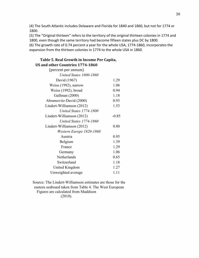
Our implied growth rates may be compatible with those of other scholars for the 1800-1860

period on which they concentrated their attention. At face value, the upper part of Table 5 seems to

show that we find higher growth, at 1.53 percent a year, over this period. Yet our growth rates for

1800-1860 will be reduced as soon as we are able to make two adjustments. The first adjustment,

already considered in Table 3, would be to raise our assumed rate of return for the highly uncertain

time around 1800, thus raising property income and total income for that starting point. The second,

discussed but not yet quantified, would be to make a rough guess at the missing pure farm profits form

      19  

that 1800 starting year, again reducing our implied growth rate for 1800-1860. Once these

adjustments are made, we suspect that the main question about our income-side estimates of nominal

national product will center more on their higher levels everywhere during the 1774-1860 era, and less

on any remaining difference in implied growth rates.

In international perspective, the income per capita in our eastern-seaboard “original thirteen”

region grew after 1800 at a rate that compared well with European growth rates for 1820-1860. So say

the comparisons in the lower part of Table 5 (though including farmers’ residual profits in 1800 would

have lowered our 1800-1860 growth rates a bit). Yet over the longer 1774-1860 period that included

the Revolutionary War our overall growth rate was slower than in Western Europe. With the help of

Table 4’s greater detail, we can identify two events that suppressed American growth in the late

eighteen century: The macro shock of the War of Independence itself, and the start of a Southern

“reversal of fortune”.

E. Revolutionary Shocks: War Damage, Diverted Trade and the Crisis at the Top

What stands out in the longer run perspective is the economic turbulence between our two

benchmark years 1774 and 1800, first with the war years themselves and then with the troubled

Confederation in the 1780s. The last quarter of the eighteenth century found the economy on a rickety

swinging bridge, a metaphor that also describes scholarly attempts to span that gap with numbers from

what has been called a statistical dark age. Like late eighteenth century France, early nineteenth

century Latin America, early twentieth century Russia, and Africa after World War II, scholars of the

early United States have had great difficulty bridging the data gap across their revolutionary upheaval

and early nation-building. On the one hand, Thomas Berry (1968, 1988), Louis Johnston and Samuel

Williamson (2010), Richard Sylla (2011) and others have emphasized the strong growth experienced

across the 1790s, perhaps due to the wisdom of Alexander Hamilton and other founding fathers and/or

due to the recovery of foreign markets. Yet, the more we come to accept their sanguine view of the

1790s, the more we must infer a true economic disaster between 1774 and 1790.

Any study attempting to measure incomes for 1774 and 1800 alone cannot quantify the depth

of any economic depression in between. Yet, we can help guide the search for the magnitude of the

Revolutionary war and post-war depression by posing a question: How deep would the per-capita

income loss have been from 1774 to 1790 if the scholars cited above are right about the growth from

1790 to 1800, and our estimates of the net decline from 1774 to 1800 are also right? This question has

      20  

eight numerical conjectures, based on our two estimates for 1800 (“baseline” and “alternative”) times

the four leading series documenting real income per capita growth from 1790 to 1800. The four series

are those by Richard Sutch, Louis Johnston and Samuel Williamson, Thomas Berry, and John

McCusker.25 All eight conjectures imply significant drops in income per capita between 1774 and

1790. Between these two years GDP per capita might have dropped 18 percent, based on Sutch and

our alternative estimate for 1800. The largest estimated drop is 30 percent, based on Berry’s series and

our baseline estimate. The estimates seem to agree with John McCusker and Russell Menard that the

“Colonists paid a high cost for their freedom”, with Allan Kulikoff that the drop in incomes was

“equal to the early years of the Great Depression”, and with their consensus that recovery was

painfully slow.26

What could have caused such sustained income losses? There is good prima facie evidence that

three related negative shocks could have been large enough to cause the deep depression between 1774

and 1790. The first was the economic destruction of the war itself, as well as the impact of nearly two

decades of hyperinflation and a dysfunctional financial system. The second negative shock consisted

of the disruptions of overseas trade during the Revolution and, after 1793, the Napoleonic Wars.27 The

shock was concentrated in the South. Available price and trade data show that the colonies, especially

in the Lower South, suffered heavy volume and value losses in trade and shipping as the war

deepened, and that they recovered only slowly and partially across the 1780s. In real per capita terms,

New England’s commodity exports rose by a trivial 1.2 percent between 1768/72 and 1791/92, rose by

a modest 9.9 percent in the Middle Atlantic, but fell by a spectacular 39.1 percent in the Upper South,

and by an even bigger 49.7 percent in the Lower South (Mancall et al. 2003 estimate an even larger 67

percent), yielding a decline of 24.4 percent for the thirteen colonies as a whole.28 The most painful of

these shocks was the loss of well over half of all trade with England between 1771 and 1791. In

addition, America lost Imperial bounties like those on the South’s indigo and naval stores, as well as

New England’s reversal from colonial bounties to prohibitive duties on its whale oil exports.

While these negative demand shocks to American commodity exports were very large,

especially for the Lower South, the initial share of exports in regional income was only about 6-7

percent in the early 1770s, according to the Shepherd-Walton export values per capita in 1768-1772

and our 1774 income estimates for the three main regions. Thus, it is hard to imagine that the huge

depression of 1774-1790 was entirely “export-led”: A 24-percent trade fall times a 6-7 percent share of

income equals no more than a 2 percent fall in income colony-wide. The numbers are bigger for the

      21  

South, where exports fell by perhaps 45 percent and the trade share was 7.1 percent, implying an

income loss of more than 3 percent. These calculations only deal with foreign trade losses; the trade

losses would be considerably higher if they included the decline in inter-colonial and subsequent inter-

state trade between 1774 and 1790. Finally, these negative trade shocks created a move back to

subsistence farming, and presumably lower agricultural productivity.

The third major negative shock involved what we call a crisis at the top, and it was felt

primarily in the coastal cities and smaller river towns. This shock was related to the trade losses, but

transcended them and could have caused much greater income losses. America’s urban centers were

severely damaged by British naval attacks, blockades, occupation, and by the eventual departure of

skilled and well-connected loyalists, especially from New York, Charleston, and Savanna. In Richard

Hildreth’s summary, “one large portion of the wealthy men of colonial times had been expatriated, and

another part impoverished”.29  

The damage to urban economic activity was considerable, and potentially enough to bring

great declines to per capita incomes, even though population kept growing. To  identify  the  extent  of  

the  urban  damage,  one  could  start  by  noting  that  the  combined  share  of  Boston,  New  York  City,  

Philadelphia,  and  Charleston  in  a  growing  national  population  shrank hugely from 5.1 percent in

1774 to 2.7 percent in 1790, recovering only partially to 3.4 percent in 1800. To the extent that

urbanization is a close correlate of levels of economic development, this big fall in the American city

population share certainly confirms what our income estimates document. There is even stronger

evidence confirming an urban crisis: the share of the mainly-urban white collar employment fell from

12.7 percent in 1774 to 8 percent in 1800; the ratio of earnings per free worker in urban jobs relative to

that of total free workers dropped from 3.4 to 1.5; and the ratio of white collar earnings per worker to

that of total free workers fell even more, from 5.2 to 1.7. This evidence offers strong support for an

urban crisis, and it also supports the view that America had not yet recovered from the Revolutionary

economic disaster even by 1800.

F. Southern Reversal of Fortune

The absolute decline of South Atlantic per capita income over the last quarter of the 18th

century and its relative decline over the next four decades stand out as a classic example of what has

come to be called reversal of fortune (Acemoglu et al. 2002). Table 4 underlines the change.

According to Richard Easterlin (1960, 1961), the South Atlantic was well behind the Northeast and the

      22  

national average by 1840, while it was well ahead of all other regions in 1774. The “Southern reversal

of fortunes” draws support from the apparent absence of any large army of poor whites in the colonial

South. We note again that what few local colonial censuses and tax records we do have reveal that

nearly all white households around 1774 were assessed as having positive wealth. The familiar image

of the South as a repository for much of the nation’s poor whites was apparently a later development.

Why the reversal of fortune for the South? A benign part of the story seems to have been that

the colonial South Atlantic was still a labor-scarce frontier with high returns to export crops. Its

decline after 1774 was echoed in two other cases of relative frontier decline: the relative decline of the

West South Central region 1840-1860 (again see Table 4), and the loss of the Pacific region’s super-

incomes after 1870. Still, the Southern reversal had multiple causes, and we do not yet know what

weights to attach to the decline of frontier super-returns, the exceptionally severe damage incurred in

the Revolutionary War, or some deeper institutional failure.

IV. Income Inequality, 1774 - 1860

While social tables are not an inherently superior way to estimate aggregate national product,

they have the clear advantage of being able to reveal the inequality of income in historical settings

where occupational labels and class rewards conveyed a great deal of income information. Thanks to

the social tables, we can now compare American income inequalities on the eve of the Revolution and

on the eve of the Civil War, whereas earlier scholarship could only draw on sketches of wealth

inequality and some scattered wage ratios.30

Incomes were much more equally distributed in colonial America than in America today, or in

other countries in the late eighteenth century. Among all American households, slaves included, Table

6 reports that the richest 1 percent had 7.1 percent of total income, and the Gini coefficient was 0.437.

Without the slaves, the top 1 percent of free households had 6.1 percent of total incomes, and the Gini

was 0.400. Compare colonial American inequality with that of the United States today, where almost

20 percent of total income accrues to the top 1 percent, and where the Gini coefficient is almost 0.50

(Atkinson, Piketty, and Saez 2011: Table 5, p. 31). The image of an egalitarian colonial America

emerges even more clearly at the regional level, in colonial New England (Gini 0.354), in the Middle

Atlantic (Gini 0.381), and, surprisingly, among free Southerners (Gini 0.328). That is, within any

      23  

American colonial region, free citizens had more equal incomes than the thirteen colonies as a whole,

the reason being that wide income gap between the Southern region and the rest.

Free American colonists also had much more equal incomes than did west Europeans at that

time. The average Gini for the four northwest European observations reported in Table 6 is 0.57,

versus that American colonial Gini of 0.437. Indeed, there was no documented place on the planet that

had a more egalitarian distribution in the late 18th century (Milanovic et al. 2011). For those who feel

that a large and strong middle class is essential for establishing institutions friendly to modern

economic growth, note that the middle of the distribution (Next 40%) received 41.6% of American

incomes in 1774, but only 27.8% in 1802 England and Wales, or 24.4% averaged over the four

European observations in Table 6. And note that the loudest revolutionary noise came from New

England, where the middle got 52.5 percent of total New England incomes.

If people had far more equal incomes in America than elsewhere, which kinds of colonists

were better off than their counterparts in Europe? Figure 1 offers a striking answer, using an Anglo-

American comparison. On the horizontal axis each society is ranked from its poorest to its richest, and

on the vertical axis their average group incomes are displayed on a log scale. It appears that an

American colonist of any percentile rank had a higher income than his or her English counterpart of

the same rank until we reach the top one percent. Indeed, it turns out that even American slaves were

above the bottom of the Anglo-American income ladder, although such comparisons fail to account for

the loss of freedom, longer hours worked, and harsher working conditions. Yet, the top incomes so

dominated in England-Wales that its national product per capita was still close to that of America. Of

course, average English incomes are likely to have matched or surpassed the American average after

our economic disaster of 1775-1790.

What about the impact of relative purchasing power on such income comparisons? As is

widely recognized, simple exchange rate conversion does not adequately account for cost of living

differences between classes and places. This familiar point has a number of important applications in

the colonial American context, and they deserve emphasis and further investigation. One is that the

cost of a standard consumption bundle probably was lower in New England than it was either in the

Southern colonies or in England and Wales. So say some recent calculations for this era. If true, then

these nominal income contrasts might be somewhat misleading. Perhaps New England -- with cheap

fish, corn, beans, rum and molasses -- was not so much poorer than the Southern colonies as the

nominal figures in Table 5 imply. This might also have been true of the Middle Colonies with its

      24  

cheap grains, exported to England and the West Indies where they were expensive (Mancall et al.

2008b). In any case, such adjustments should also deal with the relative cost and quality of housing

(Shammas 2007). Perhaps New Englanders weren’t so much worse off relative to Southerners as our

figures suggest, and perhaps workers in the Middle Atlantic were even better off compared with

English workers than our figures suggest. In contrast, an upper-class cost of living bundle, including

the cost of music, theater, and servants, must have been lower in London than in the Northern

colonies. These “real inequality” dimensions need to be explored further, but we do not expect them to

overturn the inequality contrasts shown here.31

The 1860 distribution of income for the US, for the original 13 colonies, and for each census

region is reported in Table 7, which can be compared with the 1774 results in Table 6. The main

finding is clear enough: American inequality rose everywhere over this 86-year span of history -- in

every region, among free households alone, and among slave and free combined. Furthermore, the rise

was steep. For the eastern seaboard, the “original thirteen”, the Gini rose from 0.40 (Table 6) to 0.53

(Table 7), and the share of income going to the top one percent of households rose from 7.1 to 10.0.

While income gaps widened in all parts of the eastern seaboard, the widening was most pronounced in

the South. Among slave and free household combined, the South Atlantic Gini rose from 0.46 in 1774

.60 in 1860 -- a figure much the same for the ESC (.58) and WSC (.60), and a level of inequality hard

to find anywhere in Europe or the rest of the world (Milanovic et al. 2011). Especially notable about

the South Atlantic was the enormous increase in income inequality among free households, where the

Gini rose from .33 to .51. The top-one-percent share of income increased from 6.3 to 10.1 percent

among free households in the South Atlantic, while the share going to the poorest 40 percent fell from

21.9 to 11.3 percent. Any historian looking for the rise of a poor white underclass in the Old South

will find it in this evidence.

V. Summary and Agenda

The only way to push back the quantitative frontiers of inequality, living standards, and growth

history is to adapt to the archival environments of the deep past, just as archeologists have done. Even

reaching back to the late 18th century requires the use of an eclectic array of incomplete evidence. One

of the most underexploited bodies of evidence for the early modern era consists of social and

occupational class counts allowing us to construct aggregate incomes and their distribution. Working

      25  

on that frontier, we have emerged with a rich harvest of provisional measures sketching early

American growth and inequality.

It appears that the colonists had far higher incomes in 1774 than previously thought, on

average probably greater than England, the richest country in Europe. Between 1774 and 1800

American incomes declined in real per capita terms, so that any rapid growth after 1790 failed to make

up for a very steep wartime decline and the “lost decade” of early independence. The quarter-century

decline was sufficiently big that America lost its lead to England in the income per capita rankings. In

addition, we find that free American colonists had much more equal incomes than did households in

England (and elsewhere in Europe). The colonists also had greater purchasing power than did their

English counterparts over all of the income ranks except at the top one percent.

There is abundant evidence confirming reversal of fortunes for the original southern colonies, a

region that became the South Atlantic in census terms. Our results suggest that Southern per capita

incomes were far above that of New England and the Middle Colonies in 1774, and that poor whites

were much less common there than in other colonies. It appears that the colonial South lacked the

large numbers of poor free labor that could be counted in Boston, Philadelphia, New York and lesser

coastal and river towns in the north. In short, our results suggest that mass poverty did not spread

among the Southern white population until the early 19th century. In any case, the Old South had lost

almost all of its lead in average income by 1800. Why did the Old South (to become the South

Atlantic) undergo such a spectacular reversal of fortune between 1774 and 1800? Not only do we need

to answer that question, but we also need to know more about the distribution of incomes in late

colonial and early national South, research of the sort already accumulated for Chesapeake.32

We need more work to reinforce the credibility of the estimates offered here. While we have

certainly found strong support for a steep rise in inequality over America’s first century, we do not yet

know when it happened. Future research needs to supply an inequality estimate for 1800. Only then

will we be able to separate out the role of early industrialization (1800-1860) from the turbulent first

quarter century (1774-1800). Adding an estimate of farm profits for 1800 – currently missing -- would

certainly lower our estimated 1.53 percent per annum growth rate in per capita income 1800-1860.

And new GDP deflators must be fashioned to replace the traditional ones. Finally, we are now

working on a 1870 social table, and hope that we can soon sketch the income effects of the Civil War

decade.

      26  

Table 1. Estimated American Personal Incomes, 1774 and 1800 New Middle South All 13 Colonies England Atlantic Atlantic (15 states + DC) Gross income, millions of current dollars ($4.44/£ sterling) Circa 1774 FTE free own-labor income 31.09 28.85 62.81 122.75 Ditto, part-time (see text) 28.16 27.26 58.27 113.70 Slave retained earnings 0.13   1.06   12.18   13.37  Gross property income 4.84   8.37   23.83   37.04  Gross total income 36.06   38.28   98.81   173.16   Ditto, with part-time 33.13   36.69   94.28   164.11   Circa 1800 FTE free own-labor income 73.65 84.20 87.77 245.62 Ditto, with part-time 66.57 76.91 80.88 224.36 Slave retained earnings 0.07 2.10 37.34 39.51 Gross property income 21.39 47.83 89.77 158.99 Gross total income 95.11 134.13 214.88 444.12 Ditto, with part-time 88.03 126.83 208.00 422.86 Relevant denominators Free labor force 1774 185,999 156,875 195,938 538,812 Total labor force 1774 188,230 175,655 436,136 800,021 Free population 1774 657,567 582,134 719,875 1,959,577 Total population 1774 661,563 613,685 1,101,151 2,376,399 Free labor force 1800 334,685 380,162 402,504 1,117,351 Total labor force 1800 335,500 404,900 835,590 1,575,990 Free population 1800 1,231,671 1,423,924 1,428,695 4,084,290 Total population 1800 1,233,011 1,464,548 2,222,221 4,919,780

Notes to Table 1: The estimates exclude Native Americans.

The 1800 estimates currently lack any estimate of farm operators' residual incomes beyond the implicit value of their farm labor and their property incomes (see text).

The gross property incomes for 1800 are based on middling assumptions about Southern underassessment in 1798 (see text).

The baseline estimates use the full-time assumptions of 313 days per labor year, in occupations where the primary earnings data are sub-annual (e.g. daily or monthly wage rates). The part-time assumptions retain the explicitly annual income estimates for titled and

      27  

professionals, for commercial proprietors, for manufacturing trades, servants, slaves, and household heads of unstated occupations having positive wealth. Part-time work years for explicit pay are assumed to have been only 280 days for construction workers, farm operators, and the rural unskilled. For urban unskilled and for household heads with zero wealth and unstated occupations, we assumed a work year of only 222 days.

Delaware is here included with the Middle Colonies for both years, following Alice Hanson Jones’s sample design.

Table 2. Alternative Estimates of National Income 1774 and 1800, in current $ and 1840 $ (millions)

1774 1774 1800 1800

current

$m 1840 $m current

$m 1840 $m Source

US (orig 13) 142.2 152.5 GDP: McCusker (2000) 131.7 141.6 Gross inc: Jones (1980) 173.2 185.7 444.1 305.9 Gross income: LW (2012) 164.1 176.3 422.8 291.3 “ , part-time: LW (2012) US (all) 508.7 350.3 GDP: McCusker (2000) 150.3 161.6 515.5 355.5 GDP: Mancall &Weiss (1999) 135-157 145-169 GDP: Gallman (1972) 134.8 145.0 500.1 344.9 GDP: Goldin & Lewis (1980) 132.6 142.6 Narrow GDP: Weiss (1992) 430.9 297.2 Berry (1988) 446.3 307.8 David (1996) 510.4 351.5 GDP: Mancall et al. (2003) 470.7 324.2 Gross income: LW (2012) 448.1 308.7 “ , part-time: LW (2012) New Eng. 35.5 38.2 Income: Jones (1980) 34.6 37.1 95.1 65.5 Gross income: LW (2012) Middle Atl. 36.5 39.3 Income: Jones (1980) 39.7 42.6 134.1 92.4 Gross income: LW (2012) South Atl. 59.2 63.6 Income: Jones (1980) 98.9 106.0 214.9 148.0 Gross income: LW (2012)) Lower 22.0 23.7 93.5 64.4 GDP: Mancall et al. (2003) South Atl. 94.1 64.8 Gross income: LW (2012)

Notes  to  Table  2:  (1)  Gross  inc,  Net  inc  =  personal  income,  gross  and  net  of  depreciation.  (2)  This  culled  set  omits  very  old  estimates,  and  if  a  modern  source  offers  more  than  one  estimate,  this  set  selects  the  most  recent.  It  also  selects  the  highest  in  the  Jones  range,  as  recommended  by  Gallman  and  Weiss.  (3)  We  use  the  McCusker  composite  price  index  here,  as  in  Tables  1  and  4.  

      28  

(4)  The  LW  estimates  for  1800  are  the  "baseline"  estimates.  For  our  “alternative”  estimates,  see  Table  1.  (5)  The  western  states  included  in  the  LW  “US  (all)”  estimates  are  KY  and  TN,  plus  MS  for  labor  incomes  only.    

Table 3. Alternative Property Incomes and Total Incomes, 1774 and 1800 1774 $ millions in 1774 (at $4.44/£) New Middle All 13 England Colonies South Colonies Estimated using 6% net rate of return on all NIPA-type assets and slaves Gross personal property incomes 4.840   8.372   23.830   37.042  Net personal property incomes 3.662   6.534   15.736   25.932  Total gross personal incomes 36.064   38.281   98.814   173.159  Total net personal incomes 34.886   36.444   90.719   162.049   Estimated using 8% net rate of return on all NIPA-type assets and slaves Gross personal property incomes 6.061   10.550   29.075   45.685  Net personal property incomes 4.883   8.712   20.981   34.575  Total gross personal incomes 37.285   40.459   104.058   181.802  Total net personal incomes 36.106   38.622   95.964   170.692  

1800 $ millions in 1800 New Middle All 15 states England Atlantic South and DC Baseline estimate, using 6% net rate of return on all NIPA-type assets and slaves Gross personal property incomes 21.391 47.829 89.772 158.993 Net personal property incomes 16.787 29.346 46.490 92.624 Total gross personal incomes 95.112 134.128 214.880 444.119 Total net personal incomes 90.508 115.645 171.598 377.750 Alternative estimate, using 8% net rate of return on all NIPA-type assets and slaves Gross personal property incomes 26.987 57.611 105.269 189.867 Net personal property incomes 22.383 39.129 61.987 123.498 Total gross personal incomes 100.707 143.910 230.376 474.994 Total net personal incomes 96.103 125.427 187.094 408.625  

      29  

  Table  4.  Real  Product  per  Capita,  1774  -­‐  1860          (in  1840  dollars)         1774   1800   1840   1860  New  England   61.83   56.66   129.01   181.39  Middle  Atlantic   73.81   68.73   119.68   186.65  South  Atlantic   105.70   74.29   85.49   137.75  East  North  Central       71.50   135.78  West  North  Central       79.27   136.20  East  South  Central       85.49   132.83  West  South  Central       161.65   175.30  Mountain         209.07  Pacific         501.81            "Original  thirteen"   85.26   68.22   110.93   169.18  All  USA       101.03   160.16               Implied  real  growth  rates  per  annum     1774-­‐1800   1800-­‐1840   1840-­‐1860   1744-­‐1860  New  England   -­‐0.33   2.08   1.72   1.26  Middle  Atlantic   -­‐0.27   1.40   2.25   1.08  South  Atlantic   -­‐1.35   0.35   2.41   0.31  East  North  Central       3.26    West  North  Central       2.74    East  South  Central       2.23    West  South  Central       0.41         "Original  thirteen"   -­‐0.85   1.89 2.13   0.80  All  USA   2.33   0.74    Notes  to  Table  4:  (1)  The  italicized  product  estimate  for  the  whole  United  States  in  1840  is  Thomas  Weiss’s  (1993)  “broad”  measure.  For  the  1840  italicized  regions,  the  Weiss  total  was  multiplied  by  regional  relative  products  per  capita  implied  by  Richard  Easterlin’s  (1960,  Table  A1,  variant  A)  estimates.    All  other  national  “products”  are  our  own  “part-­‐time”  estimates  of  national  personal  income.    As  noted  in  the  text,  we  use  the  “part-­‐time”  estimates  to  make  our  concept  conform  to  the  more  conventional  estimates,  even  though  we  believe  that  for  1774  and  1800  the  conventional  estimates  make  too  little  imputation  for  non-­‐market  home  production.  (2)  For  1800  we  here  used  our  “baseline”  estimate,  not  the  higher  alternative  estimate  using  an  8  percent  rate  of  return.      (3)  The  price  deflator  for  1800-­‐1860  is  that  of  Thomas  Weiss  (1993,  Table  4).    For  1774-­‐1800  we  spliced  the  David-­‐Solar  (1977)  series  onto  the  Weiss  series  at  1800.    Using  1840  =  100,  the  resulting  price  index  is  81  for  1774,  126  for  1800,  and  106  for  1860.  

      30  

(4)  The  South  Atlantic  includes  Delaware  and  Florida  for  1840  and  1860,  but  not  for  1774  or  1800.  (5)  The  “Original  thirteen”  refers  to  the  territory  of  the  original  thirteen  colonies  in  1774  and  1800,  even  though  the  same  territory  had  become  fifteen  states  plus  DC  by  1800.  (6)  The  growth  rate  of  0.74  percent  a  year  for  the  whole  USA,  1774-­‐1860,  incorporates  the  expansion  from  the  thirteen  colonies  in  1774  to  the  whole  USA  in  1860.      

Table  5.  Real  Growth  in  Income  Per  Capita,  US  and  other  Countries  1774-­1860    

(percent  per  annum)    

United States 1800-1860 David (1967) 1.29

Weiss (1992), narrow 1.06 Weiss (1992), broad 0.94

Gallman (2000) 1.18 Abramovitz-David (2000) 0.93 Lindert-Williamson (2012) 1.53

United States 1774-1800 Lindert-Williamson (2012) -0.85

United States 1774-1860 Lindert-Williamson (2012) 0.80

Western Europe 1820-1860 Austria 0.95

Belgium 1.39 France 1.29

Germany 1.06 Netherlands 0.65 Switzerland 1.18

United Kingdom 1.27 Unweighted average 1.11

Source: The Lindert-Williamson estimates are those for the eastern seaboard taken from Table 4. The West European

Figures are calculated from Maddison (2010).

 

      31  

 Table 6. Inequality in the American Colonies 1774

Region: All 13 All 13 New Middle

colonies colonies England Colonies South South Households: All Free only All All All Free only

Gini coefficient: 0.437 0.400 0.354 0.381 0.464 0.328 Income shares in % of total income Top 1% of HHs: 7.1 6.1 3.8 6.4 7.9 6.3 Top 5%: 22.2 21.6 11.4 19.3 25.6 21.3 Top 10%: 30.8 29.6 20.1 28.3 34.3 30.8 Top 20%: 47.3 43.8 35.7 43.8 49.1 42.3 Next 40%: 40.3 41.6 52.5 40.1 39.4 35.7 Bottom 40%: 12.3 14.6 11.8 16.1 11.4 21.9 Household income levels in $ (at $4.44/£ sterling) Mean: 345 406 278 289 411 620 Median: 282 377 371 274 322 585 Top 1% of HHs: 2379 2471 1059 1862 3243 3910 Top 5%: 1272 1754 631 1118 2105 2635 Top 10%: 859 1202 559 818 1410 1910 Top 20%: 776 890 496 634 1011 1312 Next 40%: 369 339 365 290 406 694 Bottom 40%: 104 230 82 117 118 199 Western Europe, as a comparison group

Region: England England (All households) & Wales & Wales Holland Netherlands

Year: 1759 1802 1732 1808 Gini coefficient: 0.522 0.593 0.610 0.563 Income shares in % of total income Top 1% of HHs: 17.5 14.6 13.7 17.0 Top 5%: 35.4 39.2 37.0 39.5 Top 10%: 45.1 48.8 50.9 51.3 Top 20%: 57.5 63.2 65.8 64.7 Next 40%: 30.0 27.8 25.6 22.8 Bottom 40%: 12.5 9.0 8.5 12.5 Household income levels Mean: £ 43.4 90.6* fl. 67.8 319.3 Median: £ 25.0 55.0 fl. 35.0 150.0 (* or £106.8 if we count government revenue, the King, and certain pensioners.)    

      32  

Notes  to  Table  6  and  Figure  1:  The  inequality  results  in  Table  6  are  based  on  the  full-­‐time  (FTE)  measures  of  incomes  at  313  days  per  year.    Inequality  would  have  been  raised  only  slightly  by  using  the  part-­‐time  work  year  assumptions  described  above.    For  example,  using  the  part-­‐time  work  years  would  yield  a  13-­‐colony  gini  coefficient  of  0.440  for  all  households,  or  0.408  for  free  households.    Figure  1  is  based  on  the  part-­‐time  work  years,  for  better  comparability  with  English  and  Dutch  inequality.    

Table  7.    The  Inequality  of  American  Household  Incomes  1860                           Percent  shares  of  total  income    

Region  Gini  coeff  

Top  1%  

Top  5%  

Top  10%  

Top  20%  

Next  40%  

Bottom  40%   Mean  Inc.  

All  households                New  Eng   0.44   6.9   20.0   31.4   48.7   37.7   13.6   989  Midd  Atl   0.48   9.3   23.5   35.7   52.8   34.8   12.5   1,083  South  Atl   0.60   12.7   31.6   45.6   63.9   28.6   7.6   742  ENC   0.39   7.2   19.0   29.2   44.8   37.8   17.4   806  WNC   0.42   7.4   20.4   31.0   46.7   38.0   15.3   799  ESC   0.58   12.4   31.6   45.0   62.1   29.8   8.1   727  WSC   0.60   15.5   34.5   47.0   63.7   28.4   8.0   931  Mountain   0.51   10.6   26.3   39.0   55.9   32.0   12.1   1,018  Pacific   0.42   6.9   19.7   30.9   47.1   38.0   14.9   2,089  USA   0.51   10.0   25.5   37.7   54.7   34.7   10.6   903  Orig  13   0.53   10.0   25.6   38.4   56.2   34.3   9.4   951  Free  households                  Midd  Atl   0.48   9.3   23.5   35.7   52.8   34.8   12.5   1,083  South  Atl   0.51   10.1   26.0   38.1   54.5   34.2   11.3   1,130  WNC   0.38   7.0   19.4   29.6   44.7   37.6   17.7   872  ESC   0.48   9.7   26.1   38.1   53.6   32.7   13.7   1,110  WSC   0.50   12.6   29.4   40.5   55.2   32.3   12.5   1,456  USA   0.47   9.3   23.8   35.4   51.6   34.8   13.6   1,035  Orig.  13   0.50   9.3   23.9   36.0   53.1   34.8   12.2   1,083  Note:  Midd  Atl  includes  DE,  and  South  Atl  includes  FL.        

           

      33  

References   Abramovitz, Moses and Paul A. David. 2000. "American Macroeconomic Growth in the Era of

Knowledge-Based Progress: The Long-Run Perspective." In Stanley Engerman and Robert Gallman (eds.), The Cambridge Economic History of the United States: Volume III: The Twentieth Century. Cambridge: Cambridge University Press, pp. 1-92.

Acemoglu, Daron, Simon Johnson, and James Robinson. 2002. “Reversal of Fortune: Geography and Institutions in the Making of the Modern World Income Distribution,” Quarterly Journal of Economics 117, 4 (November): 1231-94.

Adams, Donald R. 1968. “Wage Rates in the Early National Period: Philadelphia, 1785-1830.” Journal of Economic History 28, 3 (September): 404-426.

Adams, Donald R. 1970. “Some Evidence on English and American Wage Rates, 1790-1830.” Journal of Economic History 30, 3 (September): 499-520.

Adams, Donald R. 1982. “The Standard of Living during American Industrialization: Evidence from the Brandywine Region, 1800-1860.” Journal of Economic History 42, 4 (December): 903-917.

Adams, Donald R. 1986. “Prices and Wages in Maryland, 1750-1850.” Journal of Economic History 46, 3 (September): 625-645.

Adams, Donald R. 1992. “Prices and Wages in Antebellum America: The West Virginia Experience.” Journal of Economic History 52, 1 (March): 206-216.

Adams, T.M. 1944. Prices Paid by Vermont Farmers [1790-1940]. Bulletin 507, Burlington, Vermont: Vermont Agricultural Experiment Station, with Supplement.

Allen, Robert C., Tommy E. Murphy, and Eric B, Schneider. 2011. “The Colonial Origins of Divergence in the Americas: A Labour Market Approach”. University of Oxford Discussion Paper 559, version of 5 July.

Atack, Jeremy, and Fred Bateman. 1987. To Their Own Soil: Agriculture in the Ante Bellum North. Ames, Iowa: Iowa State University Press.

Atkinson, Anthony B., Thomas Piketty, and Emmanuel Saez. 2011. “Top Incomes in the Long Run of History,” Journal of Economic Literature 49, 1 (March): 3-71.

Berry, Thomas S. 1968. Estimated Annual Variations in Gross National Product 1789 to 1909 (Richmond, Va.: The Bostwick Press).

Berry, Thomas S. 1988. Production and Population since 1789: Revised GNP Series in Constant Dollars. Richmond, Va.: The Bostwick Press.

Blodget, Samuel. 1806. Economica: A Statistical Manual for the United States of America. Reprint: New York, August Kelley, 1964.

Carr, Lois G., Russell R. Menard and Lorena S. Walsh. 1991. Robert Cole’s World: Agriculture and Society in Early Maryland (Chapel Hill: University of North Carolina Press).

Carter, Susan et al. (eds.). 2006. The Historical Statistics of the United States: Millennial Edition. Five volumes. New York: Cambridge University Press.

Clemens, Paul G.E. and Lucy Simler. 1988. “Rural Labor and the Farm Household in Chester County, Pennsylvania, 1750-1820”. In Stephen Innes (ed.), Work and Labor in Early America. Chapel Hill: University of North Carolina Press, pp. 106-143.

Crafts, N. F. R. (1987), “British economic growth, 1700-1850: Some difficulties of interpretation,” Explorations in Economic History 24 (3): 245-68.

      34  

Craig, Lee A. 1991. “The Value of Household Labor in Antebellum Northern Agriculture”. Journal of Economic History 51, 1 (March): 67-81.

David, Paul A. 1967. “The Growth of Real Product in the United States before 1840: New Evidence and Controlled Conjectures.” Journal of Economic History 27, 2 (June).

David, Paul A. 1996. “Real income and economic welfare growth in the early Republic, or, another try at getting the American story straight.” Discussion Papers in Economic and Social History, 5 (Oxford University).

David, Paul A. and Peter Solar. 1977. “A bicentenary contribution to the history of the cost of living in America.” Research in Economic History 2: 1-80.

Davis, Joseph H. 2004. “An Annual Index of U.S. Industrial Production, 1790-1915.” Quarterly Journal of Economics 119, 4 (November 2004): 1177-215.

Eardley-­‐Wilmot,  John.  1972.  Historical  View  of  the  Commission  for  Enquiring  into  the  Losses,  Services,  and  Claims  of  the  American  Loyalists,  at  the  Close  of  the  War  between  Great  Britain  and  her  Colonies  in  1783.  London:  J.  Nichols,  Son,  and  Bentley,  1815.  Reprinted,  Boston,  Gregg  Press.

Easterlin, Richard A. 1960. “Interregional Differences in Per Capita Income, Population, and Total Income, 1840-1950,” in Trends in the American Economy in the Nineteenth Century. Princeton, N.J.: Princeton University Press, for the National Bureau of Economic Research.

Easterlin,  Richard  A.    1961.  “Regional  Income  Trends,  1840-­‐1950.”  In  Seymour  E.  Harris    (ed.),  American  Economic  History.  New  York:  McGraw-­‐Hill,  pp.  525-­‐547.  

Egnal, Marc. 1975. “The Economic Development of the Thirteen Continental Colonies, 1720 to 1775.” William and Mary Quarterly, 3rd series, 32: 191-222.

Einhorn, Robin. 2009. American Taxation, American Slavery. Chicago: University of Chicago Press.

Fogel, Robert W. and Stanley L. Engerman. 1976, updated 2006. “Slave Sales and Appraisals, 1775-1865” and “Slave Hires and Appraisals, 1775-1865.” [Computer file]. ICPSR07421-v3. Rochester, NY: University of Rochester [producer], 1976. Ann Arbor, MI: Inter-university Consortium for Political and Social Research, 2006-10-11. doi: 10.3886/ICPSR07421.

Gallman, Robert E. 1982. “Influences on the Distribution of Landholdings in Early Colonial North Carolina.” Journal of Economic History 42, 3 (September): 549-575.

Gallman, Robert E. 1992. “American Economic Growth before the Civil War: The Testimony of the Capital Stock Estimates.” In Robert E. Gallman and John Joseph Wallis (eds.), American Economic Growth and Standards of Living before the Civil War. Chicago: University of Chicago Press, pp. 79-120.

Gallman, Robert E. 1999. “Can We Build National Accounts for the Colonial Period of American History?” The William and Mary Quarterly, Third Series, 56, 1 (January): 23-30.

Gallman, Robert E. 2000. "Economic Growth and Structural Change in the Long Nineteenth Century." In Stanley L. Engerman and Robert E. Gallman (eds.), The Cambridge Economic History of the United States: Volume II: The Long Nineteenth Century. Cambridge: Cambridge University Press, pp. pp. 1-55.

Goldin, Claudia and Frank D. Lewis. 1980. “The role of exports in American economic growth during the Napoleonic Wars, 1793-1807.” Explorations in Economic History 17, 1 (January): 6-25.

      35  

Hildreth,  Richard,  1849.  The  History  of  the  United  States  of  America,  from  the  Discovery  of  the  Continent  to  the  Organization  of  Government  under  the  Federal  Constitution.  Three  volumes.  New  York,  Harper  &  brothers.  

Hoffman, Philip T., David Jacks, Patricia Levin, and Peter H. Lindert. 2002. “Real Inequality in Western Europe since 1500.” Journal of Economic History 62, 2 (June): 322-355.

Homer, Sidney and Richard Sylla. 1991. A History of Interest Rates. New Brunswick: Rutgers University Press.

Hoppit, Julian. 1996. “Political Arithmetic in Eighteenth-Century England”. Economic History Review 49, 3 (August): 516-540.

Irwin, Douglas and Richard Sylla (eds.). 2011. Founding Choices. Chicago: University of Chicago Press for the NBER.

Jasanoff,  Maya.  2011.  Liberty’s  Exiles:  American  Loyalists  in  the  Revolutionary  World.  New  York:  A.A.  Knopf.

Johnston, Louis D. and Samuel H. Williamson. 2010. “What was the U.S. GDP then?” MeasuringWorth at http://www.measuringworth.org/usgdp/.

Johnston, Louis D. and Samuel H. Williamson. n.d. “Appendix: New Estimates of GDP, 1790 to present,” unpublished.

Jones, Alice Hanson. 1977. American Colonial Wealth. Three volumes. New York: Arno Press. Jones, Alice Hanson. 1980. Wealth of a Nation to Be. New York: Columbia University Press. Kulikoff, Allan. 1986. Tobacco and Slaves: The Development of Southern Cultures in the

Chesapeake 1680–1800. Chapel Hill: University of North Carolina Press. Kulikoff, Allan. 2005. “The Economic Crisis of the Revolutionary Era,” paper presented at the

Annual Conference of the Program in Early America Economy and Society, October. Kuznets, Simon. 1976. “Demographic Aspects of the Size Distribution of Income: An Exploratory

Essay.” Economic Development and Cultural Change 25 (October): 1-94. Lebergott, Stanley. 1964. Manpower in Economic Growth: The American Record Since 1800.

New York: McGraw-Hill. Lindert, Peter H. and Jeffrey G. Williamson. 1982. “Revising England’s Social Tables, 1688-

1812.” Explorations in Economic History 19, 4 (October): 385-408. Lindert, Peter H. and Jeffrey G. Williamson. 1983. “Reinterpreting  Britain's  Social  Tables,  

1688-­‐1913.”  Explorations  in  Economic  History  20,  1  (January),  pp.  94-­‐109.   Lindert, Peter H. and Jeffrey G. Williamson. 2011. “American Incomes before and after the

Revolution”. NBER Working Paper 17211 (July). Maddison, Angus. 2007. www.ggdc.net/maddison/Historical .../horizontal-file_03-2007. Maddison, Angus. 2010. www.ggdc.net/maddison/Historical .../horizontal-file_02-2010. Main, Jackson Turner. 1965. The Social Structure of Revolutionary America. Princeton:

Princeton University Press. Mancall, Peter C., Joshua L. Rosenbloom, and Thomas Weiss. 2003. “Conjectural Estimates of

Economic Growth in the Lower South, 1720 to 1800.” in William Sundstrom and Timothy Guinnane (eds.), History Matters: Economic Growth, Technology, and Population. Stanford, Cal.: Stanford University Press, pp. 389-424.

Mancall, Peter C., Joshua L. Rosenbloom, and Thomas Weiss. 2008a. “Exports and the Economy of the Lower South Region, 1720-1770.” Research in Economic History 25: 1-68.

Mancall, Peter C., Joshua L. Rosenbloom, and Thomas Weiss. 2008b. “The Role of Exports in the Economy of Colonial North America: New Estimates for the Middle Colonies.”

      36  

NBER Working Paper 14334, National Bureau of Economic Research, Cambridge, Mass. (September).

Mancall, Peter C. and Thomas Weiss. 1999. “Was Economic Growth Likely in Colonial British North America?” Journal of Economic History 59: 17-40.

Margo,  Robert.  1990.  Wages  and  Labor  Markets  in  the  United  States,  1820-­1860.  Chicago:  University  of  Chicago  Press.

McCusker, John J. 2000. “Estimating Early American Gross Domestic Product.” Historical Methods 33, 3 (Summer): 155-159.

McCusker,  John.  2001.  How  Much  Is  That  in  Real  Money?  A  Historical  Commodity  Price  Index  for  Use  as  a  Deflator  of  Money  Values  in  the  Economy  of  the  United  States.  Second  Edition.  Worcester,  MA:  American  Antiquarian  Society.

McCusker, John J. 2006. “Colonial Statistics.” In Susan G. Carter, Michael Haines, Alan Olmstead, Richard Sutch, and Gavin Wright, Historical Statistics of the United States: Earliest Times to the present. Millennial Edition. Cambridge: Cambridge University Press, Chapter Eg, pp. 5-627 to 5-650.

McCusker, John J. and Russell Menard. 1985. The Economy of British America, 1607-1789. Chapel Hill, N.C.: University of North Carolina Press.

Milanovic, Branko, Peter H. Lindert, and Jeffrey G. Williamson. 2011. “Pre-Industrial Inequality.” Economic Journal 121 (March): 255–272.

Price, Jacob M. 1974. “Economic Function and the Growth of American Port Towns in the Eighteenth Century.” Perspectives in American History 8: 121-186.

Pitkin, Timothy. 1817. A statistical view of the commerce of the United States of America: its connection with agriculture and manufactures: and an account of the public debt, revenues, and expenditures of the United States. With a brief review of the trade, agriculture, and manufactures of the colonies, previous to their independence. Accompanied with tables, illustrative of the principles and objects of the work. Second edition. New York: James Eastburn & Co.

Rothenberg, Winifred B. 1985. “The Emergence of a Capital Market in Rural Massachusetts, 1730-1838”. Journal of Economic History 45, 4 (December): 781-808.

Seaman,  Ezra.  1852.  Essays  on  the  Progress  of  Nations.  New  York:  Scribner.  Shammas, Carole. 2007. “The Housing Stock of the Early United States: Refinement Meets

Migration”. William and Mary Quarterly 64, 3 (July): 549-590. Shepherd, James F. and Gary M. Walton. 1976. “Economic Change after the American

Revolution: Prewar and Postwar Comparisons of Maritime Shipping and Trade.” Explorations in Economic History 13, 4 (November): 397-422.

Simler, Lucy. 1990. “The Landless Worker: An Index of Economic and Social Change in Chester County Pennsylvania, 1750-1820”. The Pennsylvania Magazine of History and Biography 114, 2 (April): 163-199.

Simler, Lucy. 2007. “’She Came to Work’: The Female Labor Force in Chester County, 1750-1820”. Early American Studies 5, 2: 427-453.

Smith, Billy Gordon. 1981. “The Material Lives of Laboring Philadelphians, 1750 to 1800”. William and Mary Quarterly, Third Series, 38, 2 (April): 164-202.

Smith, Billy Gordon. 1984. “Inequality in Colonial Philadelphia: A Note on Its Nature and Growth.” William and Mary Quarterly 3rd series 41, 4 (October): 629-645.

Smith, Billy Gordon. 1990. The “Lower Sort”: Philadelphia’s Laboring People, 1750-1800. Ithaca, N.Y.: Cornell University Press.

      37  

Soltow, Lee. 1989. Distribution of Wealth and Income in the United States in 1798. Pittsburgh: Pittsburgh University Press.

Sutch, Richard. 1975. “The Treatment Received by American Slaves: A Critical Review of the Evidence Presented in Time on the Cross.” Explorations in Economic History 12 (October): 335-438.

Sylla, Richard E. 2011. “Financial Foundations: Public Credit, the National Bank, and Securities Markets.” In Douglas A. Irwin and Richard E. Sylla (eds.), Founding Choices: American Economic Policy in the 1790s. Chicago: University of Chicago Press, pp. 59-88, esp. pp. 81-83.

Trescott, Paul. 1960. “The United States Government and National Income 1790-1860.” In William N. Parker (ed.), Trends in the American Economy in the Nineteenth Century. Princeton, N.J.: Princeton University Press, pp. 337-63.

Tryon, Rolla M. 1917. Household Manufactures in the United States. New York, A. M. Kelley, reprint 1966.

United States Bureau of Labor Statistics. 1929. The History of Wages in the United States from Colonial Times to 1928. Washington: Government Printing Office.

United States Department of Commerce, Bureau of the Census. 1976. Historical Statistics of the United States: Colonial Times to 1970. Washington: Government Printing Office.

Wade, Richard D. 1964. Slavery in the Cities. New York: Oxford University Press. Walsh, Lorena S. 2010. Motives of Honor, Pleasure, & Profit: Plantation Management in the

Colonial Chesapeake, 1607-1763. Chapel Hill: University of North Carolina Press. Warden, Gerard B. 1976. “Inequality and Instability in Eighteenth-Century Boston: A

Reappraisal.” Journal of Interdisciplinary History 6: 585-620. Weiss, Thomas. 1992. “U.S. Labor Force Estimates and Economic Growth, 1800-1860.” In

Robert E. Gallman and John J. Wallis (eds.), American Economic Growth and Standards of Living before the Civil War. Chicago: University of Chicago Press, pp. 19-78.

Weiss, Thomas. 1993a. “Long-term Changes in U.S. Agricultural Output per Worker, 1800-1900.” Economic History Review 46, 2 (May): 324-341.

Weiss, Thomas. 1993b. “Estimates  of  Gross  Domestic  Output  for  the  United  States,1800  to    1860.”  University  of  Kansas,  unpublished  (July).  

Weiss, Thomas. 1994. “Economic Growth before 1860: Revised Conjectures.” In Thomas Weiss and Donald Schaefer (eds.), American Economic Development in Historical Perspective. Stanford, Stanford University Press, pp. 11-27.

Williamson, Jeffrey G. 1977. “Strategic  Wage  Goods,  Prices  and  Inequality,”  American       Economic  Review  66,  1  (March):  29-­‐41.  Williamson,  Jeffrey  G.  and  Peter  H.  Lindert.  1980.  American  Inequality:  A  Macroeconomic  

History.  New  York:  Academic  Press.  Wright, Carroll D. 1885. “Historical Review of Wages and Prices 1752-1860,” from the

Sixteenth Annual Report of the Massachusetts Bureau of Statistics of Labor. Boston: Wright & Potter.

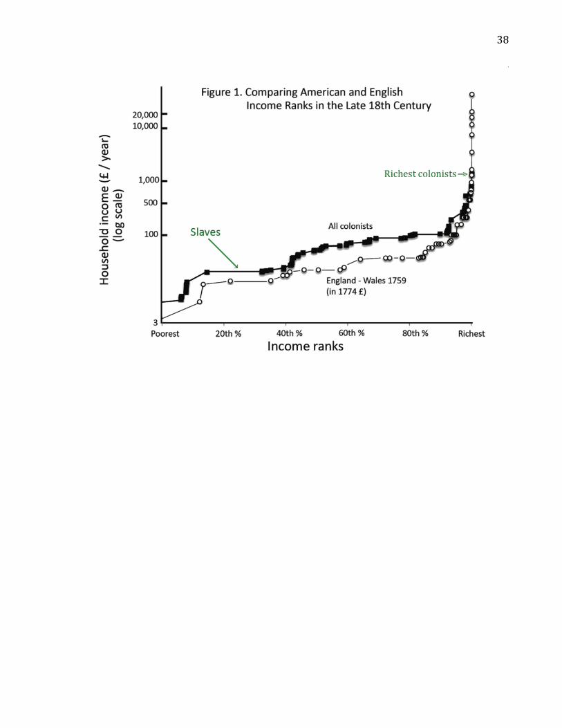
      38  

      39  

Endnotes                                                                                                                1  The  term  “reversal  of  fortune”  was  made  popular  by  Acemoglu,  Johnson,  and  Robinson  

(2002).  2  See Lindert and Williamson (1982, 1983), and Milanovic, Lindert, and Williamson (2011).  3 One of these imaginative efforts was constructed by colonial Governor James Glen of South

Carolina in 1751 (cited in McCusker 2006) and one by Samuel Blodget (1806: p. 99). They

appear to have been readers of the English political arithmeticians, whose writings accelerated

with the growing needs to finance wars. On the rise of the quantification culture in late-18th

century England, see Hoppit (1996). 4  The  debate  over  slave  maintenance  and  its  share  of  the  market  wage  is  extensive,  

especially  for  1850  and  1860.  See  “Slave  earnings  retention  1774  &  1800.doc”  at  

http://gpih.ucdavis.edu.    5 The  shares  of  the  313-­‐day  full  year  that  seem  most  plausible  as  a  conventional  “part  time”  measure  of  work  for  pay  outside  the  home  are:     1.00  (100%  of  313  days)  for  those  households  with  the  head  employed  in  the  professions,  commerce,  and  skilled  manufacturing  artisanal  jobs,  and  for  slave  households;     0.89  (280  days)  for  households  with  the  head  employed  in  construction  trades,  rural  unskilled  workers,  and  (to  understate  total  annual  days  a  bit)  farm-­‐operator  households;  and     0.71  (222  days)  for  households  headed  by  free  urban  unskilled  laborers  and  zero-­‐wealth  household  heads  of  unknown  occupation.    This  “sensitivity  analysis”  range  is  certainly  wide  enough  to  cover  such  estimates  for  England:  1760 and 1771 averaged 278 days; and 1800 280 days (Broadberry et al. 2012, Table 12). For  1774,  these  part-­‐time  assumptions  yield  the  following  ratios  of  part-­‐time  to  full-­‐time  total  incomes  (labor  plus  property):           New     4  Middle       Thirteen         England   Colonies   South     Colonies  

Free  h’holds   0.918     0.957     0.948     0.943     All  h’holds   0.919     0.958     0.954     0.948    

      40  

                                                                                                                                                                                                                                                                                                                                                                 These  ratios  imply  that  our  use  of  “full-­‐time”  estimates  will  not  explain  away  the  gap  

between  our  income  estimates  and  those  of  others  for  1774. 6 See Jones (1977, 1980) and her ISPCR data file 7329 at the Inter-University Consortium for

Political and Social Research at the University of Michigan. 7 In a set of side experiments, we tried to replicate Jones’s A*-weighted estimates using her own

data and her own procedures. In no case did we achieve exact replication, and for one regional

wealth total, we were off by 4 percent. We cannot find the source of this discrepancy, but

suspect that she had to take some shortcuts in the pre-spreadsheet era that we have not

understood. Despite the discrepancy, we feel confident of both her estimates and ours. See the

“property incomes 1774” files at http://gpih.ucdavis.edu for the details. 8 See in particular Jones (1980, pp. 61ff). 9 There are only meager data on colonial interest rates, i.e. the net opportunity cost of holding

real capital. For estimates near the 1774 benchmark, see Homer and Sylla (1991, pp. 276-279).

Near the 1800 benchmark, federal government bonds had a market yield of 6.94 percent per

annum, while New England municipals yielded 6.13 percent (Homer and Sylla 1991, p. 286).

Winifred Rothenberg (1985, p. 790) notes that 6 percent was the “Lawful Interest” stipulated by

colonial law, but that “beginning in 1785, interest rates began to climb to 7, 8, and 9 percent”.

In personal communication, Farley Grubb notes late colonial evidence that could argue for

either a 5 percent or a 6 percent rate on government borrowing. 10 The use of a zero rate on changes in producer perishables and crops adheres to a referee’s

objection to our initial assumption that all probated stocks of such perishables were used up in a

year, thus adding a 94 percent depreciation rate to the 6 percent interest forgone. Our initial

assumption added slightly to the gross national income estimates for 1774, though of course it

added nothing to the net national income. 11 The best introduction to the quantitative dimensions of the 1798 direct tax returns is still that

of Lee Soltow (1989). For the underlying political history, see Einhorn (2009). 12 Warned in advance by Gerard Warden’s (1976) investigation of the Massachusetts 1771 tax

rolls, we found implausibly low assessments not only on those rolls but also in the Philadelphia

1772 returns supplied to us by Billy Gordon Smith and in the 1786 New York City returns

supplied to us by Herbert Klein. We found those tax rolls useful for identifying occupational

      41  

                                                                                                                                                                                                                                                                                                                                                                 coverage, including occupations revealed by the presence or absence of each asset type, but not

for the assessed values themselves. 13 Lee Soltow (1989, pp. 37, 256-257) cites correspondence he found in the Oliver Wolcott

papers showing that for 518 Connecticut properties sold in 1798, the average ratio of US-

assessed value to market value was 0.845. 14 See the Excel file “1798-1800 property totals” at http://gpih.ucdavis.edu. 15 The ad valorem tax rate as a share of the Fogel-Engerman slave values (1976, updated 2006)

resembles the share of slaves that were reported. This again suggests that the undercount of

slaves was the main mechanism for understatement of Southern taxable wealth. The slave

undercount was common to all states in 1798, though over 60% of the 1800-census slaves were

reported in Connecticut, New York, and Pennsylvania, whereas less than 40% were reported in

New Jersey, Kentucky, and Tennessee. 16 The algebra of adjustment is as follows. We observe the ratio of total assessed values, South

to North (As/An) = 0.381/0.619. Under the upper bound assumption, the regional ratio of true

market values (Rs/Rn) = 0.577/0.423. Within the regions, the relationships of assessed to

market value are As = (1-Us) Rs, or An = (1-Un) Rn, where the U’s are the shares of

underassessment. The 1799 market value study suggested that Un = 0.155 in the North. These

values imply that the market value of Southern real estate Rs = 2.6226 times As, so that the

underassessment rate Us = 0.619. (Just by coincidence, this matches the Northern share of

assessments.)

When Tables 1 and 2 introduce estimates of nominal income based on our middle

assumption, one can add $9.547 million to get the result obtainable from the upper bound

assumption for 1800, or subtract the same amount for the lower bound result. 17 See Lebergott (1964), Margo (1990), the American Almanacs for 1856-1861, Craig (1991),

and our Excel files for 1860 in the American Incomes folder at http://gpih.ucdavis.edu. 18 In this passage, “wealth” means household net worth. See the http://gpih.ucdavis.edu file on

total property incomes for 1774. 19 See Homer and Sylla (1991) p. 271 and passim. 20 See the interest rate literature cited in endnote xvi above.

      42  

                                                                                                                                                                                                                                                                                                                                                                 21 Jones’s conjectural range was given in her Wealth of a Nation to Be (1980), p. 62. Robert

Gallman and Thomas Weiss have preferred her top wealth-income ratio, 3.5 to one, and that is

used in Table 3’s display of her estimates. Decomposing our aggregate 13-colony wealth-

income ratio of 1.89 into regional wealth/income ratios for 1774, we estimated the ratio at 0.96

for New England, 1.80 for the Middle Colonies, and 2.25 for the South. 22 See Homer and Sylla (1991, pp. 274-296). 23 Lucy Simler’s detailed study of Chester County, Pennsylvania found that farm operators’

families supplied 60 percent of farm labor in 1799, with the rest being hired farm labor. For

1774, she implied 67 percent (Simler 1990, p. 197, Table 3). The only alternative to

extrapolating from Chester County to the whole nation is to assume that the 1860 shares (Atack

and Bateman 1987, pp. 43-44) applied to 1800. We are exploring this option so as to estimate

farmers’ pure profits in 1800. 24  The FTE estimate, assuming everybody in the labor force worked 313 days a year, would be

$5,712 million. Yet we would not apply such an FTE assumption to the economy of 1860, even

though we feel it could be valid for 1774 or 1800, because there is evidence that non-market

home production had dropped across the antebellum years.  25  See  Series Ca11, Series Ca16, and Series Ca17 in the Historical Statistics of the United States

2006, and McCusker (2000).  26 See McCusker and Menard (1985, p. 374) and Kulikoff (2005, p. 27). 27 As Shepherd and Walton (1976) have noted, the loss of trade in the 1780s was domestic as

well as overseas, because the loose Confederation that preceded federal union briefly allowed

the new states to tax interstate trade. We concentrate here, however, on the larger and longer

shocks to trade with Britain and its possessions. 28 Shepherd and Walton (1976: especially Table 5 and the surrounding text). The Mancall et al.

(2008, Table 1) estimate for the Lower South refers to the twenty years 1770-1790. 29 Hildreth’s summary (1849, vol. III, pp. 465-466) is cited by McCusker and Menard (1985, p.

365).

An estimated 60,000 free persons (3.1 percent of the free population) and 15,000 slaves

(3.6 percent of the slave population) had left as of the early 1790s (Jasanoff 2011, pp. 351-358).

The losses to the American economy were presumably much greater than the losses that the

      43  

                                                                                                                                                                                                                                                                                                                                                                 departing loyalists experienced themselves. A high estimate of loyalist claims presented to His

Majesty for losses in American rebellion came to $1,053,024  at  the  $4.44  exchange  rate,  or  

about  0.6%  of  the  1774  income  of  the  13  colonies  (Eardley-Wilmot 1815, reprinted 1972,

Appendix VIII). Of course, this ignores the human capital that the new republic lost. 30  For  the  vast  1960s-­‐1970s  literature  on  early  wealth  inequality,  see  Williamson  and  

Lindert  (1980).    For  the  wage  ratios,  see  the  same  source  and  the  important  update  by  

Robert  Margo  (1990).  31 For the specific contrast of consumer prices between New England and other regions, see the

file “Massachusetts vs. England and WV” at http:// gpih.ucdavis.edu, and also Allen, Murphy,

and Schneider (2011, Table 3). On the more general subtlety about class- and place-specific

costs of living, see Williamson (1977) and Hoffman et al. (2002). England’s lower interest

rates may also have implied a lower user cost of capital than in the colonies. 32 See, for example, Kulikoff (1986), Carr et al. (1991), and Walsh (2010). See also Robert

Gallman’s (1982) study of Perquimans County, North Carolina.