line-of-sight observables algorithms for the helioseismic and...

Solar PhysicsDOI: 10.1007/•••••-•••-•••-••••-•

Line-of-sight observables algorithms for the

Helioseismic and Magnetic Imager (HMI)

Instrument onboard the Solar Dynamics

Observatory (SDO) tested with IBIS observations

Sebastien Couvidat1·

Sebastian P. Rajaguru2· Richard Wachter3

· Kasiviswanathan Sankarasubramanian2·

Jesper Schou1· Philip H. Scherrer1

Received: 5 July 2011

c© Springer ••••

Abstract The Helioseismic and Magnetic Imager (HMI) instrument producesline-of-sight observables (Doppler velocity, magnetic field strength, Fe i linewidth,linedepth, and continuum intensity) as well as vector-magnetic-field maps at thesolar surface. The accuracy of the line-of-sight observables is contingent uponthe quality of the observables algorithm used to translate HMI filtergrams of anobservables sequence into observables quantities. Using one hour of high-cadenceimaging spectropolarimetric observation of a sunspot in the Fe i line at 6173 Athrough the Interferometric BI-dimensional Spectrometer (IBIS) and the Milne-Eddington inversion of the corresponding Stokes vectors, we test the accuracy ofthe observables algorithm currently implemented in the HMI pipeline at StanfordUniversity: the so-called MDI-like algorithm. We also compare this algorithm toothers that may be implemented in the future in an attempt at improving theaccuracy of HMI observables: a least-squares fit with a Gaussian profile, a least-squares fit with a Voigt profile, and the use of second Fourier coefficients in theMDI-like algorithm.

Keywords: Sun: helioseismology, Instrument: SDO/HMI

1. Introduction

The Helioseismic and Magnetic Imager instrument (HMI; Schou et al., 2011)onboard the Solar Dynamics Observatory satellite (SDO) makes measurements,

1 W.W. Hansen Experimental Physics Laboratory491 S Service Road, Stanford UniversityStanford, CA 94305-4085, USAemail: [email protected] Indian Institute of Astrophysics, Bangalore, India3 Germany

SOLA: ms.tex; 6 July 2011; 15:35; p. 1

S. Couvidat et al.

in the absorption line Fe i centered at the in-air wavelength 6173.3433 A (e.g.Norton et al., 2006; Dravins, Lindegren, and Nordlund, 1981), of the motionof the solar photosphere to study solar oscillations, and of the polarization tostudy all three components of the photospheric magnetic field. HMI samplesthe neutral iron line at six positions (wavelengths) symmetrical around the linecenter at rest. The line-of-sight (LOS) observables are produced every 45 s andare: the Doppler velocity at the solar surface, the LOS magnetic field strength,the Fe i linewidth, the linedepth, and the continuum intensity. These observablesare calculated using 12 filtergrams: images taken at 6 wavelengths and 2 polar-izations (left-circular and right-circular polarizations, hereafter LCP and RCP).Unlike the Michelson Doppler Imager (MDI) instrument on which HMI is based,the observables calculations are performed on the ground at Stanford University,and not on board the spacecraft. This allows for more flexibility regarding whichobservables algorithm to apply, and makes reprocessing of these observablespossible in the eventuality that a better algorithm is later implemented. OnJune 8, 2007, the sunspot NOAA AR10960 was observed by the InterferometricBI-dimensional Spectrometer (IBIS; Cavallini 2006) instrument installed at theDunn Solar Telescope of the National Solar Observatory in Sacramento Peak(New Mexico, USA). The full Stokes profile (I,Q,U, and V) of the Fe i linewas scanned and imaged for 7 h at a cadence of 47.5 s, close to the HMIcadence (see Rajaguru et al., 2010, for details on these IBIS data processingand calibration). These IBIS images have a spectral and spatial resolutions of25 mA and 0.165” respectively (i.e. a spatial resolution three times better thanHMI), and the Fe i line was sampled at 23 different wavelengths. We select a1 hour-long observation (the first hour) out of the 7 observation hours, to keeponly the best seeing interval and to match the time interval selected for theMilne-Eddington inversion of the Stokes vectors (Skumanich and Lites, 1987).

The IBIS observations present some advantages over the HMI ones becausethe iron line is scanned at 23 wavelengths instead of 6. This allows for aninterpolation of the line profiles at each pixel on a finer wavelength grid: wecan therefore simulate HMI observations by applying the filter transmissionprofiles to these interpolated Fe i lines, and test the accuracy of not only Dopplervelocity and magnetic-field strength but also the linewidth, linedepth, and con-tinuum intensity returned by the MDI-like algorithm. We can also test otherobservables algorithms, like a least-squares fit with an appropriate Fe i profile.Moreover the Sun-Earth radial velocity varied little during the IBIS observationtimespan (from −120.98 m s−1 to −95.43 m s−1 during the 1h-long interval,compared to a 358 m s−1 change for the HMI-Sun radial velocity over thesame timespan on June 8, 2011). Another consideration for using IBIS data andtheir Milne-Eddington inversion is that, at the time of writing, the full Stokes-vector inversion data of HMI have not yet been officially released: the code vfisv(Borrero et al., 2010) is being fine-tuned. However, the spatial resolution of IBISis different from HMI, a fact that needs to be factored in when analysing the IBISresults: because, among others, of convective blueshift (depending on how wellgranules are resolved), a different spatial resolution translates into a differentFe i line profile. In Section 2 we describe the MDI-like algorithm currentlyimplemented in the HMI pipeline, in Section 3 we describe other observables

SOLA: ms.tex; 6 July 2011; 15:35; p. 2

LOS Algorithms For HMI

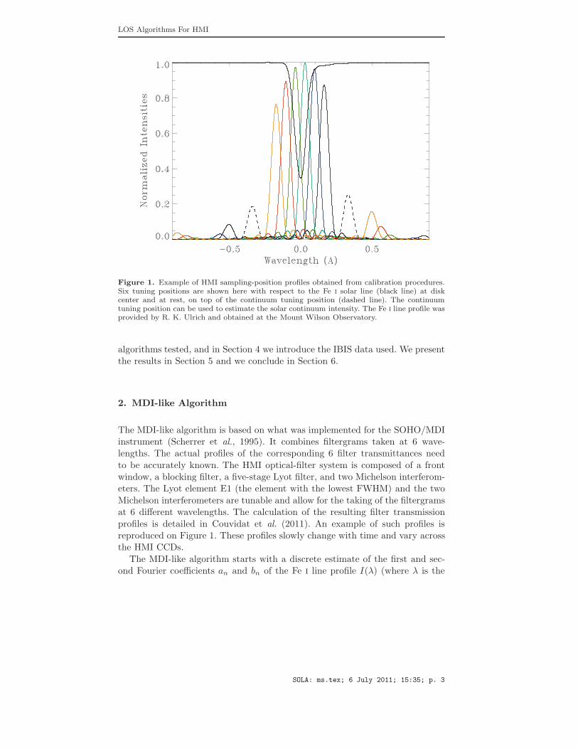
Figure 1. Example of HMI sampling-position profiles obtained from calibration procedures.Six tuning positions are shown here with respect to the Fe i solar line (black line) at diskcenter and at rest, on top of the continuum tuning position (dashed line). The continuumtuning position can be used to estimate the solar continuum intensity. The Fe i line profile wasprovided by R. K. Ulrich and obtained at the Mount Wilson Observatory.

algorithms tested, and in Section 4 we introduce the IBIS data used. We presentthe results in Section 5 and we conclude in Section 6.

2. MDI-like Algorithm

The MDI-like algorithm is based on what was implemented for the SOHO/MDIinstrument (Scherrer et al., 1995). It combines filtergrams taken at 6 wave-lengths. The actual profiles of the corresponding 6 filter transmittances need

to be accurately known. The HMI optical-filter system is composed of a frontwindow, a blocking filter, a five-stage Lyot filter, and two Michelson interferom-eters. The Lyot element E1 (the element with the lowest FWHM) and the two

Michelson interferometers are tunable and allow for the taking of the filtergramsat 6 different wavelengths. The calculation of the resulting filter transmission

profiles is detailed in Couvidat et al. (2011). An example of such profiles isreproduced on Figure 1. These profiles slowly change with time and vary acrossthe HMI CCDs.

The MDI-like algorithm starts with a discrete estimate of the first and sec-ond Fourier coefficients an and bn of the Fe i line profile I(λ) (where λ is the

SOLA: ms.tex; 6 July 2011; 15:35; p. 3

S. Couvidat et al.

wavelength):

a1 =2

T

∫ +T

2

−T

2

I(λ) cos

(

2πλ

T

)

dλ ; b1 =2

T

∫ + T

2

−T

2

I(λ) sin

(

2πλ

T

)

dλ (1)

a2 =2

T

∫ +T

2

−T

2

I(λ) cos

(

4πλ

T

)

dλ ; b2 =2

T

∫ + T

2

−T

2

I(λ) sin

(

4πλ

T

)

dλ (2)

where T is the “period” of the line profile, taken to be the FWHM of thetunable Lyot element E1 (nominally 344 mA). Assuming that the solar linehas a Gaussian profile:

I(λ) = Ic − Id exp

[

−(λ − λ0)

2

σ2

]

(3)

where Ic is the continuum intensity, Id is the linedepth, λ0 is the Doppler shift,and σ is related to the linewidth, the Doppler velocity v can be expressed as:

v =dv

dλ

T

2πatan

(

b1

a1

)

(4)

with dv/dλ = 299792458.0/6173.3433 = 48562.4 m/s/A. The second Fouriercoefficients could also be used:

v2 =dv

dλ

T

4πatan

(

b2

a2

)

(5)

The linedepth Id is equal to:

Id =T

2σ√

π

√

a21 + b2

1 exp

(

π2σ2

T 2

)

(6)

while σ is equal to:

σ =T

π√

6

√

alog

(

a21 + b2

1

a22 + b2

2

)

(7)

If the linewidth Lw of the Fe i line is defined as its FWHM, then Lw = 2√

ln(2)σ.HMI samples the Fe line at only 6 points and the Fourier coefficients are

therefore approximated as sums, for instance:

a1 ≈2

5

5∑

j=0

Ij cos

(

2π2.5 − j

6

)

(8)

The MDI-like algorithm calculates these an and bn values separately for theLCP and RCP polarizations. Applying Equation (4) to the estimates of the firstFourier coefficients, two estimates of the Doppler velocity are obtained: vLCP

and vRCP (for, respectively, LCP and RCP).

SOLA: ms.tex; 6 July 2011; 15:35; p. 4


However the HMI filter transmission profiles are not delta functions, thediscrete approximations to the Fourier coefficients are not perfect because ofa reduced number of sampling points, and the Fe i line does not have a Gaussianprofile. Therefore, the Doppler velocities vLCP and vRCP need to be corrected.To this end we use look-up tables obtained from a realistic model of the Fei line profile at rest. This profile is shifted in wavelength to simulate a givenDoppler velocity. At each shift, the line profile is multiplied by the 6 filtertransmission profiles, and the corresponding integral values are calculated. TheMDI-like algorithm is then applied. Therefore, the Doppler velocity returned bythe algorithm is a function of the actual (input) Doppler velocity. The inversefunction is called look-up table (table is a misnomer and is a legacy of theMDI implementation). Because the filter transmission profiles vary across theHMI CCDs, look-up tables also vary with the CCD pixel location. The tablesare linearly interpolated at vLCP and vRCP, producing the corrected Dopplervelocities VLCP and VRCP. In the rest of this paper, we call 1st Fourier-coefficientMDI-like algorithm the use of the 1st Fourier coefficients to estimate the Dopplervelocities, and their subsequent correction with look-up tables.

Unfortunately, the calibration of the HMI filter profiles shows some residualerrors (at the percent level) on the transmittances. Therefore, the look-up tablesare imperfect. The SDO orbital velocity is known very accurately, and it is pos-sible to use it to, partly, improve the tables. This additional step is implementedin the LOS observables code of the HMI pipeline, but will be ignored in thisarticle.

Finally, the VLCP and VRCP velocities are combined to produce a Doppler-velocity estimate:

V =VLCP + VRCP

2(9)

while the LOS magnetic field strength B is:

B = (VLCP − VRCP)Km (10)

Where Km = 1.0/(2.0× 4.67 · 10−5 × 0.000061733433× 2.5× 299792458.0) for aLande g-factor of 2.5 (Norton et al., 2006).

An estimate of the continuum intensity Ic is obtained by “reconstructing” thesolar line from the Doppler-shift estimate, linewidth, and linedepth:

Ic =1

6

5∑

j=0

[

Ij + Id exp

(

−(λ − λ0)

2

σ2

) ]

(11)

where λ0, Id, and σ are the values retrieved by Eqs (4), (6), and (7).

3. Other Observables Algorithms Tested

Observables algorithms other than the MDI-like algorithm based on 1st Fouriercoefficients are also applied to the 1-hour averaged and wavelength-interpolated

SOLA: ms.tex; 6 July 2011; 15:35; p. 5

S. Couvidat et al.

LCP and RCP IBIS line profiles (see next section): the MDI-like algorithm withthe 2nd Fourier coefficients, a least-squares fit with a Gaussian-line profile, anda least-squares fit with a Voigt profile.

Before the launch of SDO it was planned to use both the first and secondFourier coefficients when computing all the HMI LOS observables. The secondFourier coefficients are already used by the MDI-like algorithm to derive thelinewidth, linedepth, and continuum intensity, but not for the Doppler velocityand magnetic field. Unfortunately, using the second Fourier coefficients turnedout to be more difficult than anticipated (in particular there was a significantnumber of saturated pixels where the magnetic field was large, and the 2ndFourier-coefficient velocities differed significantly from the 1st Fourier-coefficientones). Because of tight time constraints it was decided to postpone the implemen-tation of the second Fourier-coefficients algorithm. The result is that currentlyonly half the information available is used, and therefore the rms variation onthe Doppler velocity due to photon noise is

√2 larger than it could be. A possible

improvement to the current implementation of the MDI-like algorithm would beto include these second Fourier coefficients: the impact of such an inclusion isdiscussed here.

The MDI-like algorithm (with 1st and/or 2nd Fourier coefficients) is compu-tationally very fast: there is no fit involved, only a combination of 6 wavelengthsfollowed by a linear interpolation. That is a reason why this algorithm waspreferred over least-squares fits. However, because the look-up tables are com-puted for a reference Fe i line profile obtained in the quiet Sun, the algorithm isexpected to fare poorly in regions of strong magnetic field. Conversely, a least-squares fit with a reasonable model of the Fe i line profile is expected to providemore accurate results, because this line profile is adjusted during the fit to reflectthe presence of magnetic fields. The simplest model of Fe i line used here is aGaussian profile. This profile results from Doppler broadening alone, and as suchis a poor approximation to the actual iron line (which also displays a significantasymmetry). A more elaborate model is the Voigt profile: a convolution betweena Gaussian profile (thermal broadening) and a Lorentzian profile (produced byradiative and collisional broadenings). It is more representative of the actual Fei line profile than a Gaussian, even though it is still symmetrical around thecentral wavelength at rest. For convenience, and to speed up the computations,an analytical expression to the Voigt-Hjerting function was used (Tepper Garcia,2006):

I(x) = Ic − Id e−x2

[

1 −a

√πx2

(

(4x2 + 3)(x2 + 1) e−x2

−(2x2 + 3)

x2sinh(x2)

)]

(12)Where x = (λ − λ0)/σ, λ0 is the Doppler shift, σ is the linewidth of the

Gaussian part of the Voigt profile, Ic is the continuum intensity, and Id is relatedto (but is not equal to) the linedepth. This expression is an approximation tothe first order in a, the so-called damping parameter, and is strictly valid fora << 1. Least-squares fits of two observed Fe i line profiles (one from the Kitt-Peak Atlas, one provided by R. Ulrich from Mount Wilson observatory and at

SOLA: ms.tex; 6 July 2011; 15:35; p. 6


solar disk center) return a value for a in the range 0.2−0.25. This is close to thea = 0.23 quoted by Bell and Meltzer (1959). Here we set a = 0.225 (other valueswere tested for comparison). It can be argued that such a large a value mightproduce a non-negligible error when using the anaytical expression of TepperGarcia (2006).

4. IBIS Data

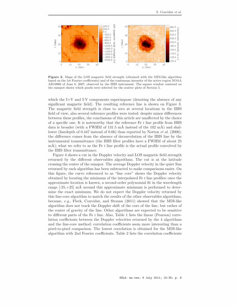
Rajaguru et al. (2010) describe with further details the IBIS data and theirMilne-Eddington inversion utilized here. We select the first hour of data, cor-responding to the best seeing interval. The format of the initial datacube is512 × 512 × 23 × 4 × 79, where the first two dimensions refer to the Cartesiancoordinates at the solar surface (the original 1024 × 1024 IBIS data have beenrebinned by a factor 2), the next dimensions are the number of wavelengthsamples (23) and of Stokes parameters (4), and the last dimension is the num-ber of time steps (this datacube covers 1.03 hours at a cadence of 47.5 s). Tocompare the LOS magnetic field strength returned by the observables algorithmswith the result of the Milne-Eddington (M-E) inversion of the Stokes vector, wefurther process the IBIS data: we select a 341× 341 pixel region centered on thesunspot (same region as in Rajaguru et al., 2010), and we temporally averagethe datacube over the full hour. Moreover, we only consider the LCP (I+V) andRCP (I-V) polarizations. Therefore the processed datacube has 341×341×23×2points. At each pixel, we apply a cubic spline interpolation (and also a quadraticinterpolation for comparison) of the 23-wavelength samples, to obtain the Stokescomponents LCP and RCP on a finer wavelength grid (with a sampling rate of0.5 mA). Figure 2 shows maps of the LOS magnetic field strength (obtained withthe 1st Fourier-coefficients MDI-like algorithm) and the continuum intensity ofthe processed IBIS data. The square window centered on the sunspot shows thearea that is selected for the scatter plots of Section 5: outside this window theM-E inversion is very noisy due to low polarization signal. It is noteworthy thatno attempt was made to correct for scattered light on IBIS data: therefore, thesignal in the sunspot umbra partly comes, probably to a significant level, fromadjacent areas and especially the penumbra.

5. Results

We test the accuracy of 4 observables algorithms previously described. To sim-ulate the 12 HMI filtergrams needed to derive LOS observables, we use a set ofHMI filter transmission profiles obtained from calibration procedures and validat solar disk center. We multiply the wavelength-interpolated LCP and RCPFe i IBIS 1 hour-averaged profiles by these filter profiles, and we compute theintegral values: those are simulated HMI intensities.

To obtain the look-up tables required by the MDI-like algorithm, a referenceFe i line profile is needed. This reference profile must be the profile at rest asseen by IBIS: therefore we select a wavelength-interpolated Stokes I profile for

SOLA: ms.tex; 6 July 2011; 15:35; p. 7

S. Couvidat et al.

Figure 2. Maps of the LOS magnetic field strength (obtained with the MDI-like algorithmbased on the 1st Fourier coefficients) and of the continuum intensity of the active region NOAAAR10960 of June 8, 2007, observed by the IBIS instrument. The square window centered onthe sunspot shows which pixels were selected for the scatter plots of Section 5.

which the I+V and I-V components superimpose (denoting the absence of anysignificant magnetic field). The resulting reference line is shown on Figure 3.The magnetic field strength is close to zero at several locations in the IBISfield of view, also several reference profiles were tested: despite minor differencesbetween these profiles, the conclusions of this article are unaffected by the choiceof a specific one. It is noteworthy that the reference Fe i line profile from IBISdata is broader (with a FWHM of 131.5 mA instead of the 102 mA) and shal-lower (linedepth of 0.447 instead of 0.66) than reported by Norton et al. (2006):the difference comes from the absence of deconvolution of the IBIS line by theinstrumental transmittance (the IBIS filter profiles have a FWHM of about 25mA); what we refer to as the Fe i line profile is the actual profile convolved bythe IBIS filter transmittance.

Figure 4 shows a cut in the Doppler velocity and LOS magnetic field strengthreturned by the different observables algorithms. The cut is at the latitudecrossing the center of the sunspot. The average Doppler velocity in the quiet Sunreturned by each algorithm has been subtracted to make comparisons easier. Onthis figure, the curve referenced to as “line core” shows the Doppler velocityobtained by locating the minimum of the interpolated Fe i line profiles: once theapproximate location is known, a second-order polynomial fit in the wavelengthrange [-25,+25] mA around this approximate minimum is performed to deter-mine the exact minimum. We do not expect the Doppler velocity returned bythis line-core algorithm to match the results of the other observables algorithms,because, e.g., Fleck, Couvidat, and Strauss (2011) showed that the MDI-likealgorithm does not track the Doppler shift of the core of the line, but rather ofthe center of gravity of the line. Other algorithms are expected to be sensitiveto different parts of the Fe i line. Also, Table 1 lists the linear (Pearson) corre-lation coefficients between the Doppler velocities returned by the 4 algorithmsand the line-core method: correlation coefficients seem more interesting than apixel-to-pixel comparison. The lowest correlation is obtained for the MDI-likealgorithm with 2nd Fourier coefficients. Table 2 lists the correlation coefficients

SOLA: ms.tex; 6 July 2011; 15:35; p. 8


Figure 3. Comparison of Fe i line profiles: the black solid line is the profile from the Kitt Peakatlas obtained by the Kitt Peak-McMath Pierce telescope while the solid orange line is thereference Fe i line profile used here to calculate the look-up tables for the MDI-like algorithmand obtained from the hour-long averaging of IBIS data.

Table 1. Pearson linear correlation coefficients between theLOS Doppler velocities returned by different algorithms forthe pixels located in the square window of Figure 2.

1st Fourier 2nd Fourier Gauss Voigt

line core 80.7 24.5 76.9 76.9

1st Fourier 100.0 40.0 98.7 98.7

for the LOS magnetic field strength. In this table and in the rest of this paper,M-E LOS inversion (or M-E LOS magnetic field) refers to the magnetic fieldstrength inverted by the Milne-Eddington code and multiplied by the cosine ofthe inclination angle. Similarly to the Doppler velocity, the lowest correlationis obtained for the 2nd Fourier-coefficients MDI-like algorithm, even though thedifference in correlation coefficients between algorithms is not as large for themagnetic field.

Figure 4 shows that the 2nd Fourier-coefficient MDI-like algorithm faresrather poorly in the sunspot, compared to the other algorithms tested. In thesunspot penumbra, the Doppler velocity returned by the 2nd Fourier coefficientsis strikingly different from the velocity returned by the 1st Fourier coefficients(and also the least-squares fits), as is also evidenced by the low correlation

SOLA: ms.tex; 6 July 2011; 15:35; p. 9

S. Couvidat et al.

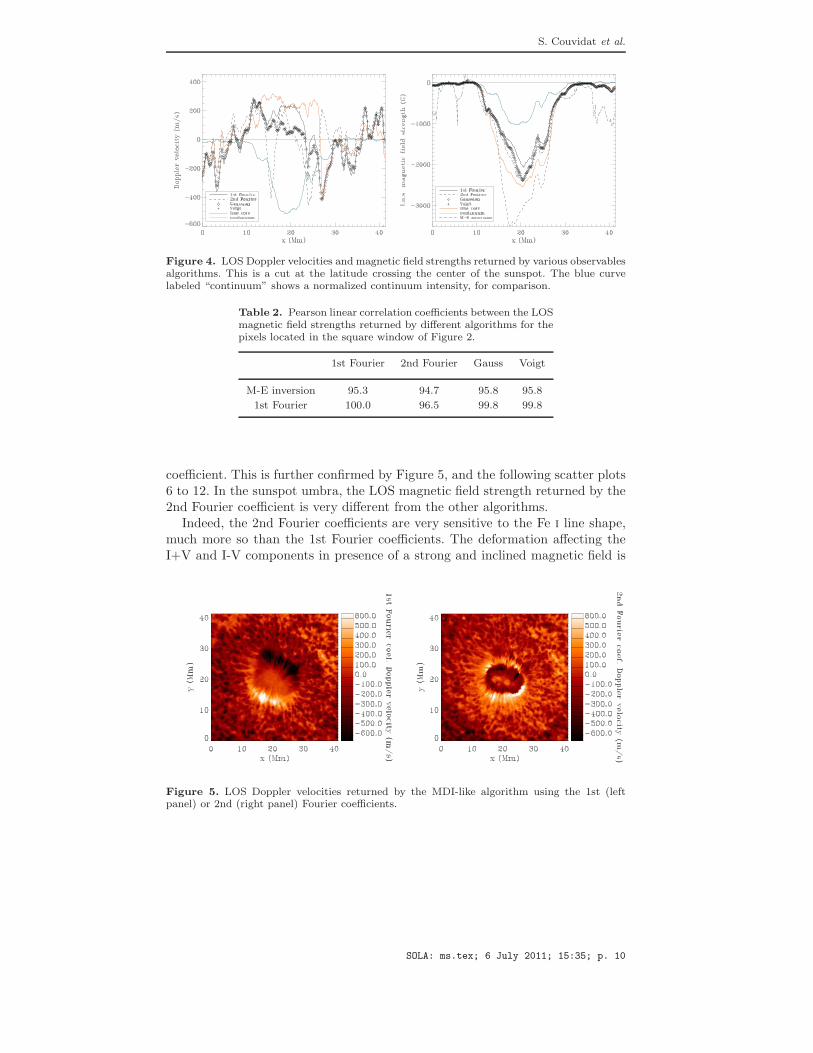
Figure 4. LOS Doppler velocities and magnetic field strengths returned by various observablesalgorithms. This is a cut at the latitude crossing the center of the sunspot. The blue curvelabeled “continuum” shows a normalized continuum intensity, for comparison.

Table 2. Pearson linear correlation coefficients between the LOSmagnetic field strengths returned by different algorithms for thepixels located in the square window of Figure 2.

1st Fourier 2nd Fourier Gauss Voigt

M-E inversion 95.3 94.7 95.8 95.8

1st Fourier 100.0 96.5 99.8 99.8

coefficient. This is further confirmed by Figure 5, and the following scatter plots6 to 12. In the sunspot umbra, the LOS magnetic field strength returned by the2nd Fourier coefficient is very different from the other algorithms.

Indeed, the 2nd Fourier coefficients are very sensitive to the Fe i line shape,much more so than the 1st Fourier coefficients. The deformation affecting theI+V and I-V components in presence of a strong and inclined magnetic field is

Figure 5. LOS Doppler velocities returned by the MDI-like algorithm using the 1st (leftpanel) or 2nd (right panel) Fourier coefficients.

SOLA: ms.tex; 6 July 2011; 15:35; p. 10


Figure 6. Relative errors on the LOS magnetic field strength returned by the observablesalgorithms with the LOS field strength returned by the M-E inversion. Upper left panel:MDI-like algorithm with 1st Fourier coefficients; Upper right panel: MDI-like algorithm with2nd Fourier coefficients; Lower left panel: least-squares fit with a Gaussian profile; Lower rightpanel: least-squares fit with a Voigt profile.

not reflected in the look-up tables, thus producing large errors for the secondFourier coefficients, and explaining the difficulties encountered during the com-missioning phase of SDO when trying to use these coefficients. Other algorithms(1st Fourier-coefficient MDI-like algorithm and least-squares fits) seem morerobust in presence of a strong and inclined field.

The impact of a magnetic field can be further assessed. Figure 6 shows theimpact of the inclination angle (relative to the vertical direction) of the fielddetermined by the M-E inversion on the relative error in LOS field strengthmade by each algorithm: for the 1st Fourier-coefficient MDI-like algorithm andthe least-squares fits, the error increases (in absolute value) when the inclinationangle increases (for angles larger than about 50 − 60 degrees correspondingto the penumbra). To obtain this plot only the pixels for which the absolutevalue of the field strength is larger than 150 Gauss and that are located insidethe window shown on Figure 2 were kept, thus avoiding the noisiest values.The low inclination angles correspond to umbral signal (partly contaminated bypenumbral signal due to scattering). None of the observables algorithm seemsto show any dependence to the azimuth angle of the magnetic field. Figure 7shows the impact of the inclination angle on the difference in Doppler velocity

SOLA: ms.tex; 6 July 2011; 15:35; p. 11

S. Couvidat et al.

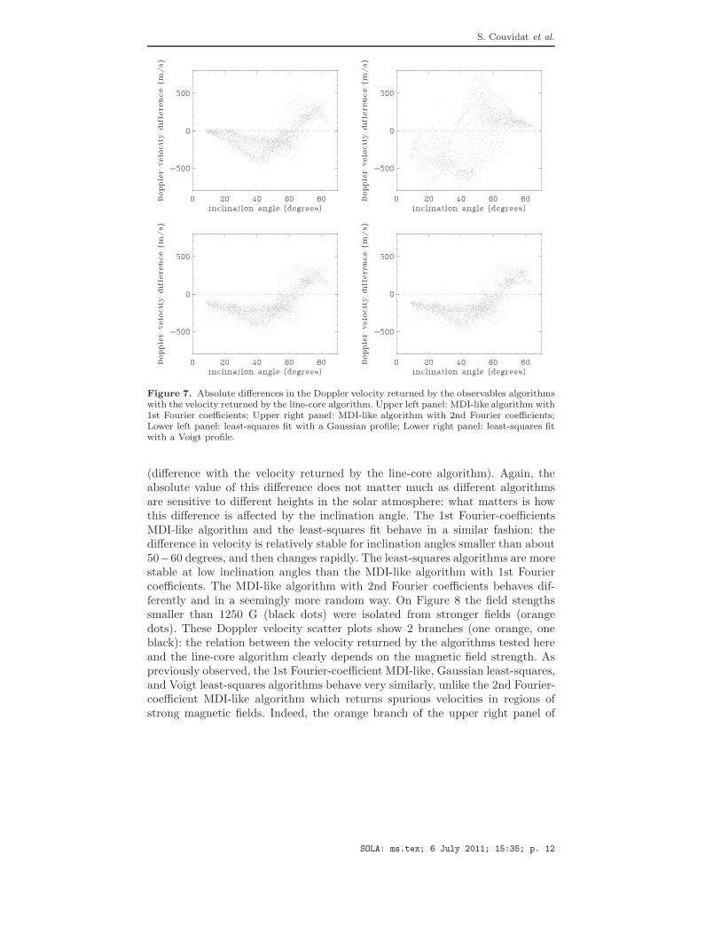
Figure 7. Absolute differences in the Doppler velocity returned by the observables algorithmswith the velocity returned by the line-core algorithm. Upper left panel: MDI-like algorithm with1st Fourier coefficients; Upper right panel: MDI-like algorithm with 2nd Fourier coefficients;Lower left panel: least-squares fit with a Gaussian profile; Lower right panel: least-squares fitwith a Voigt profile.

(difference with the velocity returned by the line-core algorithm). Again, theabsolute value of this difference does not matter much as different algorithmsare sensitive to different heights in the solar atmosphere: what matters is howthis difference is affected by the inclination angle. The 1st Fourier-coefficientsMDI-like algorithm and the least-squares fit behave in a similar fashion: thedifference in velocity is relatively stable for inclination angles smaller than about50−60 degrees, and then changes rapidly. The least-squares algorithms are morestable at low inclination angles than the MDI-like algorithm with 1st Fouriercoefficients. The MDI-like algorithm with 2nd Fourier coefficients behaves dif-ferently and in a seemingly more random way. On Figure 8 the field stengthssmaller than 1250 G (black dots) were isolated from stronger fields (orangedots). These Doppler velocity scatter plots show 2 branches (one orange, oneblack): the relation between the velocity returned by the algorithms tested hereand the line-core algorithm clearly depends on the magnetic field strength. Aspreviously observed, the 1st Fourier-coefficient MDI-like, Gaussian least-squares,and Voigt least-squares algorithms behave very similarly, unlike the 2nd Fourier-coefficient MDI-like algorithm which returns spurious velocities in regions ofstrong magnetic fields. Indeed, the orange branch of the upper right panel of

SOLA: ms.tex; 6 July 2011; 15:35; p. 12


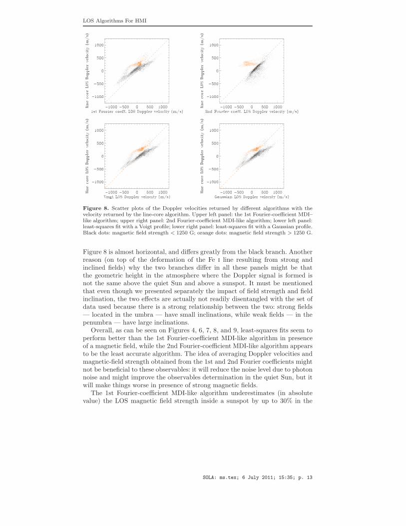
Figure 8. Scatter plots of the Doppler velocities returned by different algorithms with thevelocity returned by the line-core algorithm. Upper left panel: the 1st Fourier-coefficient MDI–like algorithm; upper right panel: 2nd Fourier-coefficient MDI-like algorithm; lower left panel:least-squares fit with a Voigt profile; lower right panel: least-squares fit with a Gaussian profile.Black dots: magnetic field strength < 1250 G; orange dots: magnetic field strength > 1250 G.

Figure 8 is almost horizontal, and differs greatly from the black branch. Anotherreason (on top of the deformation of the Fe i line resulting from strong andinclined fields) why the two branches differ in all these panels might be thatthe geometric height in the atmosphere where the Doppler signal is formed isnot the same above the quiet Sun and above a sunspot. It must be mentionedthat even though we presented separately the impact of field strength and fieldinclination, the two effects are actually not readily disentangled with the set ofdata used because there is a strong relationship between the two: strong fields— located in the umbra — have small inclinations, while weak fields — in thepenumbra — have large inclinations.

Overall, as can be seen on Figures 4, 6, 7, 8, and 9, least-squares fits seem toperform better than the 1st Fourier-coefficient MDI-like algorithm in presenceof a magnetic field, while the 2nd Fourier-coefficient MDI-like algorithm appearsto be the least accurate algorithm. The idea of averaging Doppler velocities andmagnetic-field strength obtained from the 1st and 2nd Fourier coefficients mightnot be beneficial to these observables: it will reduce the noise level due to photonnoise and might improve the observables determination in the quiet Sun, but itwill make things worse in presence of strong magnetic fields.

The 1st Fourier-coefficient MDI-like algorithm underestimates (in absolutevalue) the LOS magnetic field strength inside a sunspot by up to 30% in the

SOLA: ms.tex; 6 July 2011; 15:35; p. 13

S. Couvidat et al.

Figure 9. Scatter plots of the LOS magnetic-field strengths returned by different algorithmswith the LOS field strength returned by the M-E inversion. Upper left panel: the 1st (in black)and 2nd (in orange) Fourier-coefficient MDI-like algorithm; upper right panel: least-squaresfit with a Voigt profile; lower left panel: least-squares fit with a Gaussian profile; lower rightpanel: comparison between least-squares fit with a Voigt and Gaussian profile.

umbra (with an average value of ≈ 20%). On the contrary, the 2nd Fourier-

coefficients MDI-like algorithm overestimates this field strength by up to 50%.

The least-squares fit with a Gaussian or Voigt profile provides more accurate

results, but still slightly underestimates the actual LOS field strength in the

sunspot umbra (by ≈ 10% on average). A problem with least-squares fits is

that there are a few pixels — mainly in the sunspot umbra — for which the

gradient-expansion algorithm used did not converge: this issue does not arise

with MDI-like algorithms which always return a value. Overall the use of a

Voigt profile does not seem to improve the determination of the LOS observables

significantly more than what a simpler Gaussian profile does (see Figures 8 and

9: the Voigt and Gaussian profiles return very similar values). The use of a Voigt

profile with the analytical expression (4) actually makes linedepth and linewidth

more difficult to determine than with a basic Gaussian profile, because these

quantities do not appear explicitely in the equation and must be derived from

the fitted quantities Id and σ (the relation depends on the damping parameter

a).

SOLA: ms.tex; 6 July 2011; 15:35; p. 14


5.1. Other observables quantities: linewidth, linedepth, and continuum intensity

An advantage of using IBIS data sampled at 23 different wavelengths is thatafter interpolation we can also test how linewidth, linedepth, and continuumintensity returned by the observables algorithms compare to the actual ones.Figure 10 shows the linewidth returned by the different algorithms, while Figure11 shows the linedepth, and Figure 12 shows the continuum intensity. On thesethree figures, we separated the pixels with an inclination of the magnetic fieldlower than 57◦ (the median inclination) from the pixels with a more inclined fieldon the left panels, and we separated the pixels with a field strength lower than1250 G (in absolute value) from those with a stronger field on the right panels.The measured values (FWHMs, linedepths, and continuum intensities) are thosedirectly measured on the interpolated IBIS profiles: we measured separately theLCP and RCP components, and averaged the result. For the 4 algorithms thedispersion of results seems to increase with the magnetic field strength whilethe possible impact of inclined magnetic fields is more difficult to interpret,except for the linewidth determined with the MDI-like algorithm: in this case, itappears that the scatter plot is closer to a linear relation for less inclined fields.The MDI-like algorithm (using both 1st and 2nd Fourier coefficients for thesequantities) fares relatively poorly in presence of a magnetic field: it significantlyunderestimates the linewidth in the sunspot umbra and penumbra (by up to≈ 15%). This is not surprising, as the presence of an inclined field distorts theFe i line profile (with Zeeman splitting the σ components of a longitudinal fieldare contaminated by the π component when the inclination is different from 0):this profile is significantly different from the profile at rest used to generate thelook-up tables. The MDI-like algorithm also underestimates by a few percents theactual linewidth in the quiet Sun, probably because even in the quiet Sun the Fei line is not a Gaussian profile and is asymmetrical. It might be useful to producelook-up tables to correct the linewidth and linedepth, similarly to what is donefor the Doppler velocity. The least-squares fits provide more robust linewidthand linedepth, even though their scatter plots also deviate from a linear relationin the sunspot. The linedepth returned by the MDI-like algorithm shows a largedispersion relative to least-squares fits: for instance, for a measured linedepth of0.45, the MDI-like algorithm returns linedepths ranging from 0.42 to more than0.6, depending on magnetic field strength and inclination.

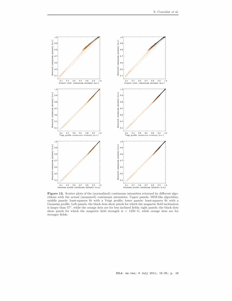
The continuum intensity returned by the MDI-like algorithm displays a seem-ingly bizarre behaviour: it first deviates from a linear relation as the normalizedcontinuum intensity decreases from 1 to about 0.5 or so (it underestimates theactual intensity), and then exhibits a linear behaviour for lower intensities. Least-squares algorithms slightly overestimate the actual continuum intensity in asunspot.

6. Conclusion

This article uses spectropolarimetric images of the solar surface obtained by theIBIS instrument to test the precision of the LOS observables returned by the

SOLA: ms.tex; 6 July 2011; 15:35; p. 15

S. Couvidat et al.

Figure 10. Scatter plots of the linewidths returned by different algorithms with the actual(measured) FWHMs. Upper panels: MDI-like algorithm; middle panels: least-squares fit witha Voigt profile; lower panels: least-squares fit with a Gaussian profile. Left panels: the blackdots show pixels for which the magnetic field inclination is larger than 57◦, while the orangedots are for less inclined fields; right panels: the black dots show pixels for which the magneticfield strength is < 1250 G, while orange dots are for stronger fields.

MDI-like algorithm currently implemented in the processing pipeline of the HMIinstrument at Stanford University. Three other observables algorithms were alsotested: the MDI-like algorithm based on the 2nd Fourier coefficients, a least-squares fit with a Gaussian profile, and a least-squares fit with a Voigt profile.It appears that, in presence of magnetic field, the least-squares fits are moreaccurate than the MDI-like algorithm (as expected). The 2nd Fourier-coefficient

SOLA: ms.tex; 6 July 2011; 15:35; p. 16


Figure 11. Scatter plots of the linedepth returned by different algorithms with the actual(measured) linedepths. Upper panels: MDI-like algorithm; middle panels: least-squares fit witha Voigt profile; lower panels: least-squares fit with a Gaussian profile. Left panels: the blackdots show pixels for which the magnetic field inclination is larger than 57◦, while the orangedots are for less inclined fields; right panels: the black dots show pixels for which the magneticfield strength is < 1250 G, while orange dots are for stronger fields.

MDI-like algorithm fares especially poorly in the sunspot, probably due to thesignificant deformation of the I+V and I-V Stokes profiles in strong and inclinedmagnetic fields. A (complicated) way to improve the MDI-like algorithms wouldbe to implement different look-up tables, depending on how a reference modelof the Fe i line varies with magnetic field strength and inclination, and usedifferent look-up tables when a strong magnetic field is detected. It is proba-

SOLA: ms.tex; 6 July 2011; 15:35; p. 17

S. Couvidat et al.

Figure 12. Scatter plots of the (normalized) continuum intensities returned by different algo-rithms with the actual (measured) continuum intensities. Upper panels: MDI-like algorithm;middle panels: least-squares fit with a Voigt profile; lower panels: least-squares fit with aGaussian profile. Left panels: the black dots show pixels for which the magnetic field inclinationis larger than 57◦, while the orange dots are for less inclined fields; right panels: the black dotsshow pixels for which the magnetic field strength is < 1250 G, while orange dots are forstronger fields.

SOLA: ms.tex; 6 July 2011; 15:35; p. 18


bly better to just abandon the MDI-like algorithm in favor of a least-squaresfit. The main issue is the speed of the algorithm: least-squares fits are ordersof magnitude slower than the MDI-like algorithm. The idea of combining 1stand 2nd Fourier-coefficient MDI-like results for Doppler velocity and LOS fieldstrength is appealing in the quiet Sun to reduce the noise level due to photonnoise, but will likely degrade the accuracy of the LOS observables in strongmagnetic fields: the 2nd Fourier-coefficient MDI-like algorithm is unreliable insunspots. Overall, despite its reduced accuracy compared to least-squares fit, the1st Fourier-coefficients algorithm is actually performing relatively well even inpresence of magnetic field. Using the results of this article it might be possibleto partly correct the LOS observables derived by this algorithm as a functionof the LOS magnetic field strength calculated. Since the IBIS data used herewere taken prior to the launch of SDO, it would also be interesting to havesimultaneous observations by HMI and IBIS, and to this end a proposal willshortly be submitted to the NSO. Finally, it should be reminded that the Fe i lineseen by IBIS is slightly different from the HMI one (different PSFs for instance),and the lines used here have been convolved by the IBIS filter transmittances:therefore, the results obtained might be slightly different from what we wouldget from the actual HMI line profile.

Acknowledgements This work was supported by NASA Grant NAS5-02139 (HMI). We

thank the HMI team members for their hard work. We also thank professor R. Ulrich for

providing us with Fe i line profiles from Mount Wilson observatory.

References

Bell, B., Meltzer, A.: 1959, Smithsonian Contribution to Astrophysics 3, 39.Borrero, J.M., Tomczyk, S., Kubo, M., Socas-Navarro, H., Schou, J., Couvidat, S., Bogart, R.:

2010, Solar Phys. in press.Cavallini, F.: 2006, Solar Phys. 236, 415.Couvidat, S., Schou, J., Shine, R.A., Bush, R.I., Miles, J.W., Scherrer, P.H., Rairden, R.L.:

2011, Solar Phys. in press.Dravins, D., Lindegren, L., Nordlund, A.: 1981, Astron. Astrophys. 96, 345.Norton, A.A., Graham, J.P., Ulrich, R.K., Schou, J., Tomczyk, S., Liu, Y., Lites, B.W., Ariste,

A. Lopez, Bush, R.I., Socas-Navarro, H., Scherrer, P.H.: 2006, Solar Phys. 239, 69.Rajaguru, S.P., Wachter, R., Sankarasubramanian, K., Couvidat, S.: 2010, ApJ 721, L86.Scherrer, P.H., Bogart, R.S., Bush, R.I., Hoeksema, J.T., Kosovichev, A.G., Schou, J., et al.:

1995, Solar Phys. 162, 129.Schou, J., Scherrer, P.H., Bush, R.I., Wachter, R., Couvidat, S., Rabello-Soares, M.C., et al.:

2011, Solar Phys. submitted.Skumanich, A., Lites, B.W.: 1987, ApJ 322, 473.Tepper Garcia, T.: 2006, MNRAS 369, 2025.Wachter, R., Schou, J., Rabello-Soares, M.C., Miles, J.W., Duvall, T.L., Jr., Bush, R. I.: 2011,

Solar Phys. in press.

SOLA: ms.tex; 6 July 2011; 15:35; p. 19

SOLA: ms.tex; 6 July 2011; 15:35; p. 20

line-of-sight observables algorithms for the helioseismic and...

Documents