linear algebra: exercisespeople.dm.unipi.it/berardu/didattica/2016-17mdal/eserciziario... · 10...

Linear Algebra: Exercises

Alessandro Berarducci, Oscar Papini

November 24, 2016

Contents

1 Linear Systems 1

2 Vector Spaces 7

3 Linear Subspaces 13

4 Linear Maps 21

5 Eigenvalues and Eigenvectors 39

6 Scalar Products 61

7 More Exercises 63

iii

iv CONTENTS

Chapter 1

Linear Systems

Exercise 1.1. Let A be the matrix

A =

1 1 1 11 1 2 22 2 3 3

.(a) Determine if the system Ax = 0 has zero, one or infinitely many solutions,

and compute a basis of the space of solutions.

(b) Is it true that the system Ax = b has a solution for any b ∈ R3? If so, provethe statement, otherwise find a counterexample.

Solution. (a) We have to find kerA. At first we row-reduce A:

1 1 1 10 0 1 10 0 0 0

1 1 1 10 0 1 10 0 1 1

1 1 1 11 1 2 22 2 3 3

(second row)− (first row)(third row)− 2(first row)

(third row)− (second row)

1

2 CHAPTER 1. LINEAR SYSTEMS

There are two pivots and two free variables, therefore the system has infinitelymany solutions. We choose x2 and x4 as free variables, and

• from x3 + x4 = 0 we get x3 = −x4;

• from x1 + x2 + x3 + x4 = 0 we get x1 = −x2.

Thus

kerA =

−x2x2−x4x4

∣∣∣∣∣∣∣∣ x2, x4 ∈ R

and a basis is

−1100

,

00−11

.

(b) Let b =

b1b2b3

be a generic vector of R3. The system Ax = b has a solution if

and only if the matrix A and the complete matrix

A =

1 1 1 1 b11 1 2 2 b22 2 3 3 b3

have the same rank. That happens if and only if the row reduced form of A,which is 1 1 1 1 b1

0 0 1 1 b2 − b10 0 0 0 b3 − b2 − b1

,has not a pivot in the third column, i.e. b3 − b2 − b1 = 0. Any vector b notsatisfying this condition, for example

b =

001

,is a counterexample for the statement. �

Exercise 1.2. Determine the number of solutions of the following systemx+ 2y − 3z = 4

4x+ y + 2z = 6

x+ 2y + (a2 − 19)z = a,

depending on the parameter a ∈ R.

3

Solution. The matrix associated to the system is1 2 −3 44 1 2 61 2 a2 − 19 a

.We get the row echelon form of the matrix subtracting the first row from thethird, and then subtracting four times the first row from the second:1 2 −3 4

0 −7 14 −100 0 a2 − 16 a− 4

.Notice that the roots of a2 − 16 = (a+ 4)(a− 4) are ±4.

• If a 6= ±4, the term a2 − 16 is not zero and we have a unique solution.

• If a = −4, the third equation of the system in echelon form becomes 0z = −8and there are no solutions.

• If a = 4, the third equation of the system in echelon form becomes 0z = 0,which is satisfied by any value of z. Therefore the system has infinitelymany solutions. �

Exercise 1.3. Determine the number of solutions of the following systemx1 + kx2 + (1 + 4k)x3 = 1 + 4k

2x1 + (k + 1)x2 + (2 + 7k)x3 = 1 + 7k

3x1 + (k + 2)x2 + (3 + 9k)x3 = 1 + 9k

depending on the parameter k ∈ R.

Solution. If we row-reduce the complete matrix of the system, we get

A =

1 k 4k + 1 4k + 10 1− k −k −k − 10 0 −k −k

.• If k 6= 0 and k 6= 1, the matrix A has three non-zero pivots in the first three

columns. Therefore the coefficients matrix is invertible, and the system hasa unique solution.

• If k = 0, the matrix A has two non-zero pivots in the first two columns,and we have only zeros in the third row. This means that the rank ofthe coefficients matrix is 2 and it is the same of the one of the completematrix, but it is not the maximum rank. Thus the system has infinitelymany solutions.


• If k = 1, the matrix A is no longer row reduced, so we can go on and get

1 1 5 50 0 −1 −20 0 0 1

.

This matrix has a pivot in the last column, which then cannot be a linearcombination of the others. In this case the system has no solutions. �

Exercise 1.4. Consider the following system, where the variables are x, y, z:

(k + 2)x+ 2ky − z = 1

x− 2y + kz = −ky + z = k.

(a) For which values of k ∈ R does the system have a unique solution?

(b) For which values of k ∈ R does the system have infinitely many solutions?If any, compute for those values of k all the solutions of the system.

Solution. An n×n system has a solution if and only if the matrix of the coefficientsand the complete matrix have the same rank; in particular, the solution is uniqueif this rank is n, and there are infinitely many solutions if this rank is less thann.

In this case, the complete matrix is

k + 2 2k −1 11 −2 k −k0 1 1 k

.

Elementary row operations change neither the set of the solutions, nor the ranksof the matrices. After some computation we get to the row echelon form:

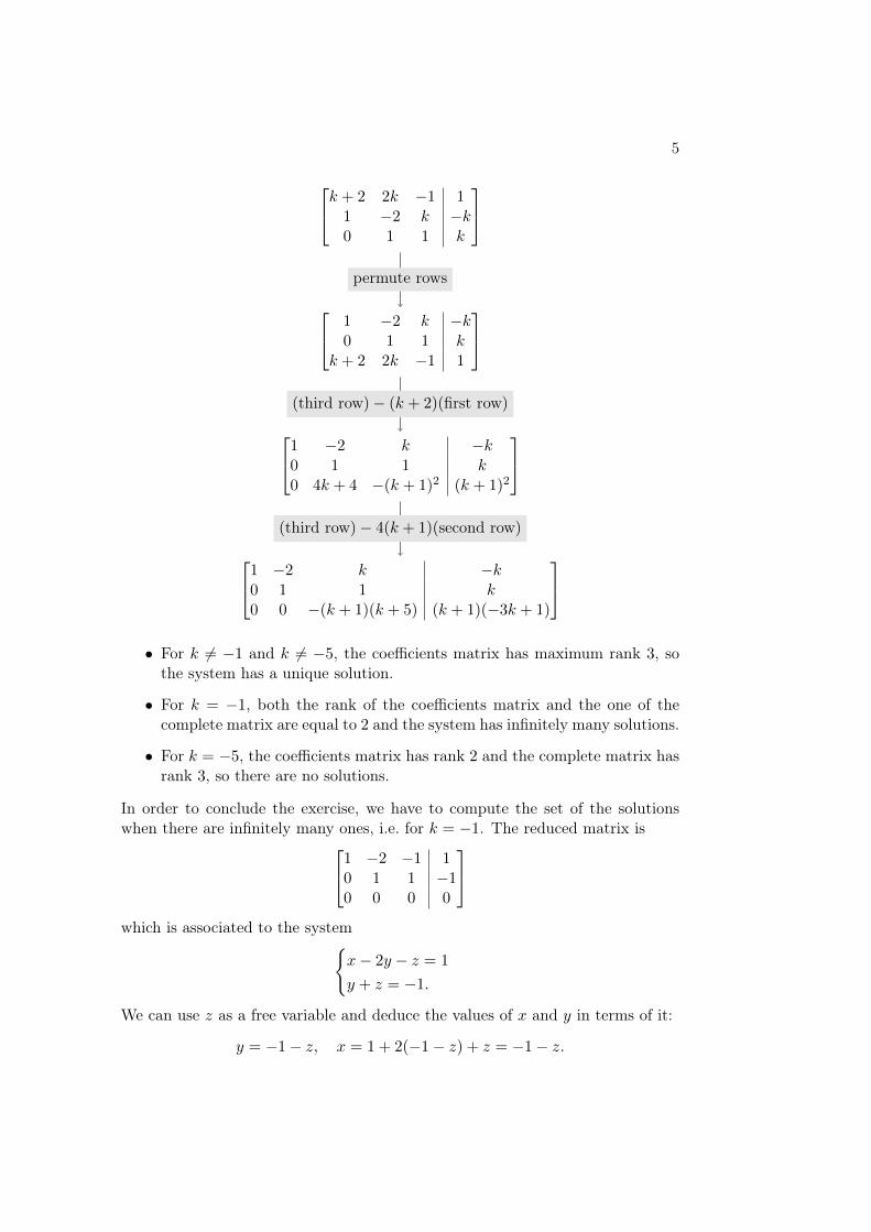
5

1 −2 k −k0 1 1 k0 0 −(k + 1)(k + 5) (k + 1)(−3k + 1)

1 −2 k −k0 1 1 k0 4k + 4 −(k + 1)2 (k + 1)2

1 −2 k −k0 1 1 k

k + 2 2k −1 1

k + 2 2k −1 11 −2 k −k0 1 1 k

permute rows

(third row)− (k + 2)(first row)

(third row)− 4(k + 1)(second row)

• For k 6= −1 and k 6= −5, the coefficients matrix has maximum rank 3, sothe system has a unique solution.

• For k = −1, both the rank of the coefficients matrix and the one of thecomplete matrix are equal to 2 and the system has infinitely many solutions.

• For k = −5, the coefficients matrix has rank 2 and the complete matrix hasrank 3, so there are no solutions.

In order to conclude the exercise, we have to compute the set of the solutionswhen there are infinitely many ones, i.e. for k = −1. The reduced matrix is1 −2 −1 1

0 1 1 −10 0 0 0

which is associated to the system{

x− 2y − z = 1

y + z = −1.

We can use z as a free variable and deduce the values of x and y in terms of it:

y = −1− z, x = 1 + 2(−1− z) + z = −1− z.


In conclusion, the set of solutions is

{(−1− λ,−1− λ, λ) | λ ∈ R}. �

Chapter 2

Vector Spaces

Exercise 2.1. (I) Find the coordinates of the vector c =

[21

]with respect to the

basis (u1, u2) of R2, where

u1 =

[32

]and u2 =

[23

].

(II) Find the coordinates of the polynomial p(x) = 2 + x in the space R[x]≤1 ofpolynomials with real coefficients and degree less than or equal to 1, with respectto the basis (q1(x), q2(x)), where q1(x) = 3 + 2x and q2(x) = 2 + 3x (in thisorder).

Solution. (I) We have to find two numbers x1, x2 ∈ R such that x1u1 +x2u2 = c,i.e.

x1

[32

]+ x2

[23

]=

[21

],

that is equivalent to solve the system[3 22 3

] [x1x2

]=

[21

].

We row-reduce the complete matrix[3 2 22 3 1

]

[3 2 20 5/3 −1/3

].

From the second equation we obtain x2 = −1/5, which we substitute in the firstequation to get, after a quick computation, x1 = 4/5. Therefore the coordinatesof c are (4/5,−1/5).(II) We use the basis (e1(x), e2(x)) of R[x]≤1, where e1(x) = 1 and e2(x) = x, totransfer the problem in R2:

• p(x) = 2 + x = 2e1(x) + e2(x) which corresponds to the vector[21

];

7

8 CHAPTER 2. VECTOR SPACES

• q1(x) = 3 + 2x = 3e1(x) + 2e2(x) which corresponds to the vector[32

];

• q2(x) = 2 + 3x = 2e1(x) + 3e2(x) which corresponds to the vector[23

].

The system to solve is

x1

[32

]+ x2

[23

]=

[21

],

which is the same of part (I): once again, the solution is (4/5,−1/5). Note thatthis does not correspond to the polynomial (4/5)+(−1/5)x: the coordinates are apair of numbers, not a polynomial, and they just mean that p(x) = (4/5)q1(x) +(−1/5)q2(x). �

Exercise 2.2. Prove the following statement, or find a counterexample: if V isa K-vector space and v1, v2, v3 ∈ V are vectors such that

(i) v1 6= 0;

(ii) v2 /∈ span(v1);

(iii) v3 /∈ span(v1, v2);

then v1, v2 and v3 are linearly independent.

Solution. The statement is true, and we will use reductio ad absurdum to prove it.Suppose that v1, v2 and v3 are linearly dependent, that is there exist x1, x2, x3 ∈ Ksuch that

x1v1 + x2v2 + x3v3 = 0 (∗)

and at least one of them is different from zero.

• If x3 6= 0, from (∗) we obtain

v3 = −x1x3v1 −

x2x3v2

which contradicts (iii).

• If x3 = 0 but x2 6= 0, (∗) becomes x1v1 + x2v2 = 0 and, since x2 6= 0, weobtain

v2 = −x1x2v1

which contradicts (ii).

• Finally, if x3 = 0 and x2 = 0, necessarily x1 6= 0; now (∗) has the formx1v1 = 0 from which we deduce v1 = 0, contradicting (i).

Since all cases brought us to an absurd, the statement is proven. �

9

Exercise 2.3. Let

v1 =

1112

, v2 =

12−11

, v3 =

0112

.(a) Is it true that v1, v2 and v3 are linearly independent, seen as vectors in R4?

Write a basis of span(v1, v2, v3) and complete it to a basis of R4.

(b) Is it true that v1, v2 and v3 are linearly independent, seen as vectors in(Z3)

4? Write a basis of span(v1, v2, v3) and complete it to a basis of (Z3)4.

Solution. (a) In order to test the linear dependence, we put the three vectors ina matrix and row-reduce it:

1 1 00 1 10 0 30 0 0

1 1 00 1 10 0 30 0 3

1 1 00 1 10 −2 10 −1 2

1 1 01 2 11 −1 12 1 2

(second row)− (first row)(third row)− (first row)

(fourth row)− 2(first row)

(third row) + 2(second row)(fourth row) + (second row)

(fourth row)− (third row)

(?)


Since in the row reduced form there are three pivots, v1, v2 and v3 are linearlyindependent over R and they are a basis of their span.

Now, to complete them to a basis of R4, we add a system of generators

A =

1 1 01 2 11 −1 12 1 2

∣∣∣∣∣∣∣∣1 0 0 00 1 0 00 0 1 00 0 0 1

and row-reduce the matrix, obtaining

1 1 00 1 10 0 30 0 0

∣∣∣∣∣∣∣∣1 0 0 0−1 1 0 0−3 2 1 00 −1 −1 0

.The pivots are in the first, second, third and fifth columns, therefore the corre-sponding columns of A, i.e. v1, v2, v3,

0100

,

form a basis of R4.(b) Over Z3, the previous row reduction is still valid until we reach the matrix(?). From there, since 3 = 0 in Z3, we can write (?) as

1 1 00 1 10 0 00 0 0

and that is the row reduced form. In this case, we have only two pivots, so thevectors are linearly dependent and a basis of span(v1, v2, v3) is (v1, v2), i.e. thevectors corresponding to the pivots.

As before, to complete it to a basis of (Z3)4 we add a set of generators and

row-reduce the resulting matrix (remember that all operations are done in Z3):

B =

1 11 21 −12 1

∣∣∣∣∣∣∣∣1 0 0 00 1 0 00 0 1 00 0 0 1

1 10 10 00 0

∣∣∣∣∣∣∣∣1 0 0 0−1 1 0 00 2 1 00 0 1 0

.The pivots are in the first, second, fourth and fifth columns, therefore the corre-sponding columns of B, i.e. v1, v2,

0100

,

0010

,

11

form a basis of (Z3)4. �

Chapter 3

Linear Subspaces

Exercise 3.1. Let K be a field, and let V = K[x]≤3. Consider the subspaceW ⊆ V given by

W = {p ∈ V | p(1) = 0}.(a) Compute dimW , justifying the answer.

(b) Compute the cardinality of W for K = Z13.

Solution. (a) We know that dimV = 4. It is clear that W is a subspace of V :

• the polynomial 0 belongs to W ;

• if p, q ∈W , then (p+ q)(1) = p(1) + q(1) = 0 + 0 = 0, so p+ q ∈W ;

• if p ∈W and λ ∈ K, then (λp)(1) = λ · p(1) = λ · 0 = 0, so λp ∈W .

Now, if p ∈ V , we can write p = ax3 + bx2 + cx+ d with a, b, c, d ∈ K, and

W = {ax3 + bx2 + cx+ d ∈ V | a+ b+ c+ d = 0}.

If we identify V with K4 through the isomorphism that sends a polynomial tothe vector of its coefficients, we can read W as a subspace of K4:

W =

abcd

∈ K4

∣∣∣∣∣∣∣∣ a+ b+ c+ d = 0

.

It is easy to see that we can use b, c and d as free variables and set a = −b−c−d;in other words

W =

−b− c− d

bcd

∣∣∣∣∣∣∣∣ b, c, d ∈ K

,

thus dimW = 3.(b) Every n-dimensional K-vector space is isomorphic to Kn, therefore if K = Z13

we have W ' (Z13)3 and its cardinality is 133. �

13

14 CHAPTER 3. LINEAR SUBSPACES

Exercise 3.2. Let

v1 =

112

, v2 =

224

, w1 =

13−2

, w2 =

0−24

be vectors in R3.

(a) Let V = span(v1, v2) and W = span(w1, w2). Find a basis of V ∩W .

(b) Complete {w1, w2} to a basis of R3.

(c) Is it possible to complete {v1, v2} to a basis of R3?

Exercise 3.3. Let V = span(v1, v2, v3) (over R), where

v1 =

1111

, v2 =

2223

, v3 =

112−1

.Let W be the subset of V which contains all and only the vectors of V that havethe first two components equal to 0.

(a) Compute dimV .

(b) Is W a subspace of V ?

(c) Compute a basis of W .

Solution. (a) We have to extract a subset of {v1, v2, v3} made of linearly indepen-dent vectors. We put the three vectors in a matrix and compute its row reducedform:

1 2 11 2 11 2 21 3 −1

1 2 10 1 −20 0 10 0 0

.Since there are three pivots, the vectors v1, v2 and v3 are linearly independentand form a basis of V , whose dimension is 3.(b) The set W is

W =

x1x2x3x4

∈ V∣∣∣∣∣∣∣∣ x1 = x2 = 0

and it is indeed a linear subspace of W .

• 0 ∈ W because 0 ∈ V (since V itself is a vector space) and the first twocomponents of 0 are zeros (actually all components. . . ).

15

• Let w1, w2 ∈W , that is w1, w2 ∈ V and

w1 =

00ab

, w2 =

00cd

for some a, b, c, d ∈ R. Then w1 +w2 ∈ V because V is a vector space, and

w1 + w2 =

00

a+ cb+ d

so it belongs to W .

• Let w ∈W and k ∈ R. With the same argument as above, kv ∈ V (becausev ∈ V ) and its first two components are k · 0 = 0, so kv ∈W .

(c) Notice that W = V ∩ Z, where Z is the set of the solutions of the system{x1 = 0

x2 = 0.

Then we look for a system of equations for V : a generic vector belongs to V ifand only if

rk

1 2 1 x11 2 1 x21 2 2 x31 3 −1 x4

< 4.

We row-reduce the matrix, obtaining1 2 1 x10 1 2 x4 − x10 0 1 x3 − x10 0 0 x2 − x1

,thus its rank is not 4 if and only if x2 − x1 = 0. Therefore W = V ∩ Z is the setof the solutions of

x2 − x1 = 0

x1 = 0

x2 = 0.

Now, by substitution we have that the first equation is redundant, because itreduces to 0 = 0. So actually W = V ∩ Z = Z and a basis of it is

0010

,

0001

. �


Exercise 3.4. In the vector space R4, consider the subspace V given by thesolutions of the system {

x+ 2y + z = 0

−x− y + 3t = 0(∗)

and the subspace W generated by the vectors

w1 =

2011

and w2 =

3−2−20

.Compute dim(V ∩W ) and dim(V +W ).

Solution. The two vectors spanning W are linearly independent, so dimW = 2.On the other hand, it is easy to show that dimV = 2, because we can choose x andy freely, and then z and t are uniquely determined. Moreover W * V because,for instance, w1 /∈ V (x = 2, y = 0, z = 1 and t = 1 is not a solution of thesystem (∗)). This means that dim(V ∩W ) < dimW strictly, that is to say thateither dim(V ∩W ) = 1 or 0. Notice that also w2 /∈ V , but this tells us nothingmore about dim(V ∩W ). Then, we have to check when a linear combination ofw1 and w2,

a

2011

+ b

3−2−20

=

2a+ 3b−2ba− 2ba

, (†)

belongs to V . By substituting the respective values in the system (∗), we obtain{(2a+ 3b) + 2(−2b) + (a− 2b) = 0

−(2a+ 3b)− (−2b) + 3a = 0

which can be simplified to {3a− 3b = 0

a− b = 0

that is equivalent to a = b. In other words, any vector of the form (†) with a = bbelongs to V ∩W ; in particular, if a = b = 1 we get the vector

5−2−11

which is not the zero vector and belongs to V ∩W , thus proving that dim(V ∩W ) ≥ 1. Since we already know that dim(V ∩W ) ≤ 1, we can conclude thatdim(V ∩W ) = 1.

17

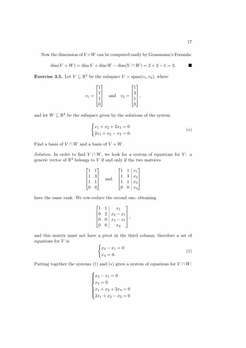
Now the dimension of V +W can be computed easily by Grassmann’s Formula:

dim(V +W ) = dimV + dimW − dim(V ∩W ) = 2 + 2− 1 = 3. �

Exercise 3.5. Let V ⊆ R4 be the subspace V = span(v1, v2), where

v1 =

1110

and v2 =

1310

,and let W ⊆ R4 be the subspace given by the solutions of the system{

x1 + x2 + 2x4 = 0

2x1 + x2 − x3 = 0.(∗)

Find a basis of V ∩W and a basis of V +W .

Solution. In order to find V ∩ W , we look for a system of equations for V : ageneric vector of R4 belongs to V if and only if the two matrices

1 11 31 10 0

and

1 1 x11 3 x21 1 x30 0 x4

have the same rank. We row-reduce the second one, obtaining

1 1 x10 2 x2 − x10 0 x3 − x10 0 x4

,and this matrix must not have a pivot in the third column; therefore a set ofequations for V is {

x3 − x1 = 0

x4 = 0.(†)

Putting together the systems (†) and (∗) gives a system of equations for V ∩W :x3 − x1 = 0

x4 = 0

x1 + x2 + 2x4 = 0

2x1 + x2 − x3 = 0


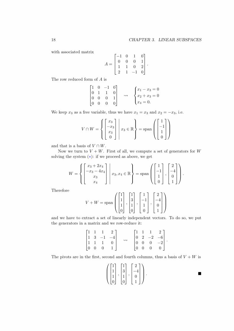
with associated matrix

A =

−1 0 1 00 0 0 11 1 0 22 1 −1 0

.The row reduced form of A is

1 0 −1 00 1 1 00 0 0 10 0 0 0

x1 − x3 = 0

x2 + x3 = 0

x4 = 0.

We keep x3 as a free variable, thus we have x1 = x3 and x2 = −x3, i.e.

V ∩W =

x3−x3x30

∣∣∣∣∣∣∣∣ x3 ∈ R

= span

1−110

and that is a basis of V ∩W .Now we turn to V + W . First of all, we compute a set of generators for W

solving the system (∗): if we proceed as above, we get

W =

x3 + 2x4−x3 − 4x4

x3x4

∣∣∣∣∣∣∣∣ x3, x4 ∈ R

= span

1−110

,

2−401

.

Therefore

V +W = span

1110

,

1310

,

1−110

,

2−401

and we have to extract a set of linearly independent vectors. To do so, we putthe generators in a matrix and we row-reduce it:

1 1 1 21 3 −1 −41 1 1 00 0 0 1

1 1 1 20 2 −2 −60 0 0 −20 0 0 0

.The pivots are in the first, second and fourth columns, thus a basis of V +W is

1110

,

1310

,

2−401

. �

19

Exercise 3.6. Consider the following subspaces of R4:

U = span

1111

,

1−11−1

and W = span

1010

,

1202

.

(a) Find a basis of U +W and a basis of U ∩W .

(b) Does it exist a subspace Z ⊆ R4 such that U ⊕ Z = W ⊕ Z = R4? If so,determine this subspace, otherwise prove that it can’t exist.

Solution. (a) We know that, if GU is a set of generators for U and GW is a set ofgenerators for W , then GU ∪GW is a set of generators for U +W , from which wecan extract a basis. Therefore we put all the generators in a matrix

1 1 1 11 −1 0 21 1 1 01 −1 0 2

and reduce it in row echelon form. The result is

1 1 1 00 2 1 00 0 0 10 0 0 0

;

the pivots are in the first, second and fourth columns, so the vectors1111

,

1−11−1

,

1202

are linearly independent and form a basis of U +W .

Now notice that the generators of U are linearly independent, and so are thegenerators of W , therefore dimU = dimW = 2. From Grassmann Formula itfollows that

dim(U ∩W ) = dimU + dimW − dim(U +W ) = 1.

thus any non-zero vector of U ∩W forms a basis of it. For example,1010

∈ U ∩W,


because it is one of the given generators of W and1010

=1

2

1111

+

1−11−1

∈ U.

(b) If we complete a basis of U to a basis of R4, the added vectors span a comple-ment of U , and the same is true for W . We are done if we can find two vectorsw1 and w2 such that both

1111

,

1−11−1

, w1, w2

and

1010

,

1202

, w1, w2

are bases of R4; the requested subspace Z exists if and only if it is possible tochoose such vectors, and in that case Z = span(w1, w2). It is easy to verify thatthe vectors

w1 =

1000

and w2 =

0100

satisfy the condition above. �

Chapter 4

Linear Maps

Exercise 4.1. Let f : R3 → R2 be a linear map such that

f

123

=

[21

]and f

234

=

[24

].

(a) Compute f

81318

.

(b) Compute the dimension of ker f .

Exercise 4.2. Let f : R2 → R3 be the linear map defined as

f

([xy

])=

x+ 2y2x+ 4yx+ ay

where a ∈ R is a parameter.

(a) Find the matrix [f ] associated to f with respect to the standard bases ofR2 and R3.

(b) For which values of a is f injective?

(c) For which values of a is f surjective?

Solution. (a) If (e1, e2) is the standard basis of R2, the i-th column of [f ] is thevector of the coordinates of f(ei) with respect to the standard basis of R3. Since

f(e1) = f

([10

])=

121

and f(e2) = f

([01

])=

24a

,21

22 CHAPTER 4. LINEAR MAPS

we have

[f ] =

1 22 41 a

.(b) The map f is injective if and only if ker f = {0}. To compute ker f , werow-reduce [f ]: 1 2

2 41 a

1 20 a− 20 0

.The corresponding system has a unique solution

[xy

]=

[00

]if a 6= 2, and infinitely

many solutions otherwise. So f is injective if and only if a 6= 2.(c) Recall that Im f = span(f(e1), f(e2)), so dim Im f ≤ 2. In particular, for anya ∈ R we have dim Im f 6= dimR3 and f is never surjective. �

Exercise 4.3. Let f : R3 → R3 be a linear map such that

f

001

=

234

, f

020

=

6810

and f

100

=

101418

.(a) Compute the dimensions of ker f and Im f .

(b) Compute f

111

.

Solution. We begin from question (b). Since f is linear, if f(v) = w then f(v/2) =w/2, so we can compute

f

010

= f

1

2

020

=1

2f

020

=1

2

6810

=

345

.This means that we know the images of all the vectors in the standard basis ofR3; these images are the columns of the matrix associated to f with respect tothe standard basis:

[f ] =

10 3 214 4 318 5 4

.Applying this matrix to the vector (1, 1, 1) we get

f

111

=

10 3 214 4 318 5 4

111

=

10 + 3 + 214 + 4 + 318 + 5 + 4

=

152127

.

23

For question (a), we notice that345

+

234

=

579

=1

2

101418

,i.e. the three columns of [f ] are linearly dependent. Thus the rank of [f ] is at mosttwo—in fact, it is exactly 2 because the second and third columns are linearlyindependent. So we can conclude that dim Im f = 2 and

dim ker f = dimR3 − dim Im f = 3− 2 = 1. �

Exercise 4.4. Let V be the real vector space R[x]≤2, whose elements are thepolynomials with real coefficients and degree less than or equal to two. Considerthe linear map L : V → V that, for any a, b, c ∈ R, sends the polynomial ax2 +bx+ c to the polynomial (3a+ 3b)x2 + (b+ c)x+ (a+ b+ 2c).

(a) Compute the dimensions of the kernel and the image of L.

(b) Decide if L is invertible and, if so, compute the image of the polynomial4x2 + x+ 1 through the inverse function.

Solution. The matrix associated to L with respect to the basis (x2, x, 1) of R[x]≤2is

[L] =

3 3 00 1 11 1 2

.We begin from question (b): we try to compute the inverse of [L] with the stan-dard algorithm. If we find an inverse, it means that L is invertible, hence bijective.In this case the answer for question (a) follows immediately: dim kerL = 0 (L isinjective) and dim ImL = 3 (L is surjective).

Recall that the inverse algorithm requires to perform row operations on thematrix 3 3 0

0 1 11 1 2

∣∣∣∣∣∣1 0 00 1 00 0 1

.It turns out that the inverse matrix does exist and it is 1/6 −1 1/2

1/6 1 −1/2−1/6 0 1/2

.In order to conclude the exercise we have to evaluate the inverse function on thepolynomial 4x2 + x+ 1. It suffices to apply the inverse matrix to the vector4

11


obtaining 1/67/6−1/6

,which corresponds to the polynomial

1

6x2 +

7

6x− 1

6. �

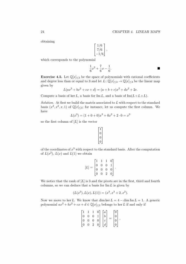
Exercise 4.5. Let Q[x]≤3 be the space of polynomials with rational coefficientsand degree less than or equal to 3 and let L : Q[x]≤3 → Q[x]≤3 be the linear mapgiven by

L(ax3 + bx2 + cx+ d) = (a+ b+ c)x3 + dx2 + 2c.

Compute a basis of kerL, a basis for ImL, and a basis of Im(L ◦ L ◦ L).

Solution. At first we build the matrix associated to L with respect to the standardbasis (x3, x2, x, 1) of Q[x]≤3; for instance, let us compute the first column. Wehave

L(x3) = (1 + 0 + 0)x3 + 0x2 + 2 · 0 = x3

so the first column of [L] is the vector1000

of the coordinates of x3 with respect to the standard basis. After the computationof L(x2), L(x) and L(1) we obtain

[L] =

1 1 1 00 0 0 10 0 0 00 0 2 0

.We notice that the rank of [L] is 3 and the pivots are in the first, third and fourthcolumns, so we can deduce that a basis for ImL is given by

(L(x3), L(x), L(1)) = (x3, x3 + 2, x2).

Now we move to kerL. We know that dim kerL = 4 − dim ImL = 1. A genericpolynomial ax3 + bx2 + cx+ d ∈ Q[x]≤3 belongs to kerL if and only if

1 1 1 00 0 0 10 0 0 00 0 2 0

abcd

=

0000

,

25

that is equivalent to the systema+ b+ c = 0

d = 0

2c = 0.

It is easy to show that the set of the solutions of this system is−αα00

∣∣∣∣∣∣∣∣ α ∈ Q

,

which is a vector subspace spanned by−1100

that corresponds to the polynomial −x3 + x2. Therefore a basis for kerL is(−x3 + x2).

The last question asks to compute a basis for Im(L ◦L ◦L). We know that aset of generators is

{(L ◦ L ◦ L)(x3), (L ◦ L ◦ L)(x2), (L ◦ L ◦ L)(x), (L ◦ L ◦ L)(1)};

let us compute these values:

• since L(x3) = x3, we also have (L ◦ L ◦ L)(x3) = x3;

• (L ◦ L ◦ L)(x2) = (L ◦ L)(x3) = x3;

• (L ◦ L ◦ L)(x) = (L ◦ L)(x3 + 2) = L(L(x3) + 2L(1))) = L(x3 + 2x2) =x3 + 2x3 = 3x3;

• (L ◦ L ◦ L)(1) = (L ◦ L)(x2) = L(x3) = x3.

It follows that

Im(L ◦ L ◦ L) = span(x3, x3, 3x3, x3) = span(x3)

and a basis for Im(L ◦ L ◦ L) is (x3). �

Exercise 4.6. Let LA : R4 → R4 be the linear map defined as LA(v) = Av, where

A =

1 2 1 02 2 0 20 1 1 −11 3 2 −1

.


(a) Find a basis of kerLA and complete it to a basis of R4.

(b) Find a basis of ImLA.

(c) Does the vector b =

18−3−2

belong to ImLA?

Solution. (a) The row reduced echelon form of A is

A =

1 0 −1 20 1 1 −10 0 0 00 0 0 0

.The set of solutions of the system associated to A is

z − 2t−z + tzt

∣∣∣∣∣∣∣∣ z, t ∈ R

,

from which we can obtain a basis of kerLA:

kerLA = span

1−110

,−2101

.

In order to complete it to a basis of R4, we row-reduce the matrix1 −2 1 0 0 0−1 1 0 1 0 01 0 0 0 1 00 1 0 0 0 1

and we take the columns corresponding to the pivots. It turns out that the pivotsare in the first four columns, so a basis of R4 is

1−110

,−2101

,

1000

,

0100

.

(b) The pivots of A are in the first two columns, so a basis of ImLA is given bythe first two columns of A:

ImLA = span

1201

,

2213

.

27

(c) It is sufficient to row-reduce the matrix1 2 12 2 80 1 −31 3 −2

and check if there is a pivot in the third column. The reduced form is

1 0 70 1 −30 0 00 0 0

,therefore b ∈ ImLA and, more precisely,

b = 7

1201

− 3

2213

. �

Exercise 4.7. Let K be a field and let V = K[x]≤3 be the space of polynomialswith degree less than or equal to 3 and coefficients in K. Consider the linear mapf : V → V defined as

f(ax3 + bx2 + cx+ d) = (a+ b)x3 + (b+ c)x2 + (c+ d)x+ (a− d).

(a) Compute a basis of ker f , a basis of Im f and a basis of ker f ∩ Im f whenK = R.

(b) Compute a basis of ker f , a basis of Im f and a basis of ker f ∩ Im f whenK = Z2.

Solution. We consider the standard basis of V given by C = (x3, x2, x, 1), andfind the matrix [f ] associated to f with respect to this basis. Recall that the i-thcolumn of [f ] is the vector of the coordinates of f(ei) with respect to C, where eiis the i-th vector of C.

• f(x3) = x3 + 1;

• f(x2) = x3 + x2;

• f(x) = x2 + x;

• f(1) = x− 1.


Therefore

[f ] =

1 1 0 00 1 1 00 0 1 11 0 0 −1

[f ] =

1 1 0 00 1 1 00 0 1 10 0 0 2

where we also row-reduced the matrix.(a) If K = R, we have that rk[f ] = 4, so ker f = {0}, Im f = V and ker f ∩Im f ={0}.(b) If K = Z2, 2 = 0, so [f ] has rank 3 and the vectors corresponding to thecolumns of the pivots of [f ] form a basis of Im f . In this case

Im f = span(f(x3), f(x2), f(x)

)= span(x3 + 1, x3 + x2, x2 + x).

In order to compute a basis of ker f , we solve the system1 1 0 00 1 1 00 0 1 10 0 0 2

xyzt

=

0000

, that is

x+ y = 0

y + z = 0

z + t = 0.

Recalling that −1 = 1 in Z2, we easily get that x = y = z = t is a solution, thus

ker[f ] = span

1111

,

from which we can recover a basis of ker f :

ker f = span(x3 + x2 + x+ 1).

Now, since dim ker f = 1, we have that either ker f ∩ Im f = {0} or ker f ∩ Im f =ker f , and the latter is true if and only if x3 + x2 + x + 1 ∈ Im f . But it is easyto show that

x3 + x2 + x+ 1 = (x3 + 1) + (x2 + x) = f(x3) + f(x) ∈ Im f,

so we can conclude ker f∩Im f = ker f and a basis is given by (x3+x2+x+1). �

Exercise 4.8. Let f : (Z7)4 → (Z7)

3 be the linear map associated to the matrix

A =

1 2 5 23 2 0 11 1 3 −1

with respect to the standard basis. Find a basis of ker f and a basis of Im f .

29

Solution. We begin reducing A to its row echelon form. Remember that thecoefficients lie in Z7, so all the operations have to be performed mod 7.

1 2 5 20 1 2 30 0 0 0

1 2 5 20 1 2 30 −1 −2 −3

1 2 5 20 3 6 20 −1 −2 −3

1 2 5 23 2 0 11 1 3 −1

(second row)− 3(first row)

(third row)− (first row)

−2(second row)

(third row) + (second row)

The pivots are in the first two columns, so these columns of A are a basis of theimage of f :

Im f = span

131

,2

21

.

For ker f , we solve the system associated to the row reduced form of A:{x+ 2y + 5z + 2t = 0

y + 2z + 3t = 0.

We choose z and t as free variables and obtain

ker f =

−z − 3t−2z − 3t

zt

∣∣∣∣∣∣∣∣ z, t ∈ Z7

= span

−1−210

,−3−301

. �


Exercise 4.9. Let K be a field and let T : K3 → K3 be the linear map associatedto the matrix

[T ] =

9 −1 7−1 5 51 −1 3

with respect to the standard basis.

(a) Determine kerT and ImT when K = Z2.

(b) Determine kerT and ImT when K = Z3.

(c) In which of the previous cases is it true that K3 = kerT ⊕ ImT?

Exercise 4.10. Let

V =

0 11 32 10 5

∈M4×2(R)

and let v1, v2 be its two columns.

(a) Find ImV and kerV .

(b) For which values of a ∈ R does the vector w =

1aaa

belong to ImV ?

(c) Find two vectors v3, v4 ∈ R4 such that (v1, v2, v3, v4) is a basis of R4.

Solution. (a) The two vectors v1 and v2 are linearly independent. This can beseen by row-reducing V , or by noticing that they are not multiple of each other.Thus (v1, v2) is a basis of ImV and its dimension is 2. It follows that dim kerV =dimR2 − dim ImV = 0, so kerV = {0}.(b) The vector w belongs to ImV if and only if the matrix

0 1 11 3 a2 1 a0 5 a

has not rank 3. Its row reduced form is

1 3 a0 1 10 0 −a+ 50 0 a− 5

,so w ∈ ImV if and only if a = 5.

31

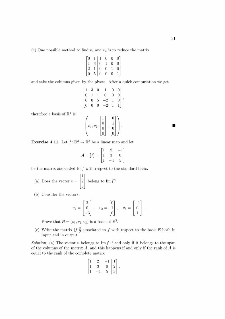
(c) One possible method to find v3 and v4 is to reduce the matrix0 11 32 10 5

∣∣∣∣∣∣∣∣1 0 0 00 1 0 00 0 1 00 0 0 1

and take the columns given by the pivots. After a quick computation we get

1 3 0 1 0 00 1 1 0 0 00 0 5 −2 1 00 0 0 −2 1 1

,therefore a basis of R4 is v1, v2,

1000

,

0100

. �

Exercise 4.11. Let f : R3 → R3 be a linear map and let

A = [f ] =

1 2 −11 3 01 −4 5

be the matrix associated to f with respect to the standard basis.

(a) Does the vector v =

123

belong to Im f?

(b) Consider the vectors

v1 =

20−3

, v2 =

010

, v3 =

−101

.Prove that B = (v1, v2, v3) is a basis of R3.

(c) Write the matrix [f ]BB associated to f with respect to the basis B both ininput and in output.

Solution. (a) The vector v belongs to Im f if and only if it belongs to the spanof the columns of the matrix A, and this happens if and only if the rank of A isequal to the rank of the complete matrix1 2 −1 1

1 3 0 21 −4 5 3

.


By using simple row operations we find that both ranks are equal to 3, so vbelongs to Im f .(b) Three vectors in a three-dimensional vector space form a basis if and onlyif they are linearly independent. To check this for v1, v2, v3, we put them in amatrix

B =

v1∣∣∣∣∣∣v2∣∣∣∣∣∣v3 =

2 0 −10 1 0−3 0 1

and compute its rank, for example by finding its row reduced echelon form. Itturns out that this rank is 3, so v1, v2 and v3 are linearly independent.(c) The matrix B computed above is actually a basis change matrix from B to thestandard basis C = (e1, e2, e3), i.e. it is the matrix [id]CB. To compute the matrixassociated to f with respect to B, we have the formula

[f ]BB = [id]BC [f ][id]CB = B−1AB.

We have to find B−1 with the usual algorithm: 2 0 −10 1 0−3 0 1

∣∣∣∣∣∣1 0 00 1 00 0 1

1 0 00 1 00 0 1

∣∣∣∣∣∣−1 0 −10 1 0−3 0 −2

and finally obtain

[f ]BB = B−1AB =

8 2 −22 3 −111 2 −2

. �

Exercise 4.12. Consider the following two ordered subsets of R3:

C =

233

,1

23

,0

01

, B =

311

,0

11

,0

01

.

Let L : R3 → R3 be the linear map given by

L

xyz

=

x+ yx+ zx+ z

.Find a basis of kerL, a basis of ImL, and write the matrix [L]BC associated to Lwith respect to the basis C in input and to the basis B in output.

Solution. The matrix associated to L with respect to the standard basis E =(e1, e2, e3) is

A = [L]EE =

1 1 01 0 11 0 1

33

and the row reduced echelon form is1 1 00 −1 10 0 0

, (∗)

therefore a basis for ImL is given by the columns where the pivots are, that is

ImL = span

111

,1

00

.

A basis for kerL can be found solving the system obtained by (∗):{x+ y = 0

−y + z = 0,

for which we choose e.g. z as a free variable and get x = −z, y = z. In conclusion

kerL = span

−111

.

In order to answer the last question, we need the basis change matrices for B andC. In fact, we have

[L]BC = [id]BE [L]EE [id]EC

or, graphically,

R3(C) R3(E) R3(E) R3(B)id L id

The vectors of the sets B and C are already written with respect of the basis E ,so we can easily get

[id]EC =

2 1 03 2 03 3 1

and [id]EB =

3 0 01 1 01 1 1

.The only thing to do is to compute [id]BE = ([id]EB)−1 with the usual algorithm3 0 0

1 1 01 1 1

∣∣∣∣∣∣1 0 00 1 00 0 1

1 0 00 1 00 0 1

∣∣∣∣∣∣1/3 0 0−1/3 1 0

0 −1 1

and finally

[L]BC =

1/3 0 0−1/3 1 0

0 −1 1

1 1 01 0 11 0 1

2 1 03 2 03 3 1

=

5/3 1 010/3 3 1

0 0 0

. �


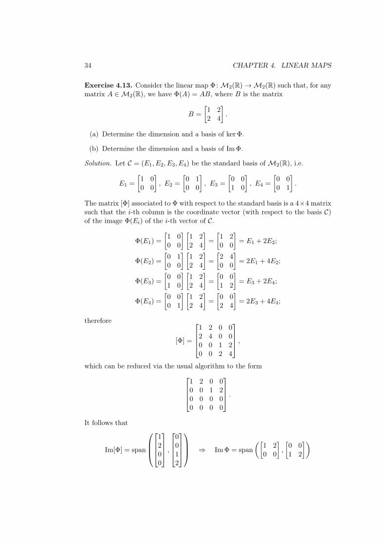
Exercise 4.13. Consider the linear map Φ: M2(R)→M2(R) such that, for anymatrix A ∈M2(R), we have Φ(A) = AB, where B is the matrix

B =

[1 22 4

].

(a) Determine the dimension and a basis of ker Φ.

(b) Determine the dimension and a basis of Im Φ.

Solution. Let C = (E1, E2, E3, E4) be the standard basis ofM2(R), i.e.

E1 =

[1 00 0

], E2 =

[0 10 0

], E3 =

[0 01 0

], E4 =

[0 00 1

].

The matrix [Φ] associated to Φ with respect to the standard basis is a 4×4 matrixsuch that the i-th column is the coordinate vector (with respect to the basis C)of the image Φ(Ei) of the i-th vector of C.

Φ(E1) =

[1 00 0

] [1 22 4

]=

[1 20 0

]= E1 + 2E2;

Φ(E2) =

[0 10 0

] [1 22 4

]=

[2 40 0

]= 2E1 + 4E2;

Φ(E3) =

[0 01 0

] [1 22 4

]=

[0 01 2

]= E3 + 2E4;

Φ(E4) =

[0 00 1

] [1 22 4

]=

[0 02 4

]= 2E3 + 4E4;

therefore

[Φ] =

1 2 0 02 4 0 00 0 1 20 0 2 4

,which can be reduced via the usual algorithm to the form

1 2 0 00 0 1 20 0 0 00 0 0 0

.It follows that

Im[Φ] = span

1200

,

0012

⇒ Im Φ = span

([1 20 0

],

[0 01 2

])

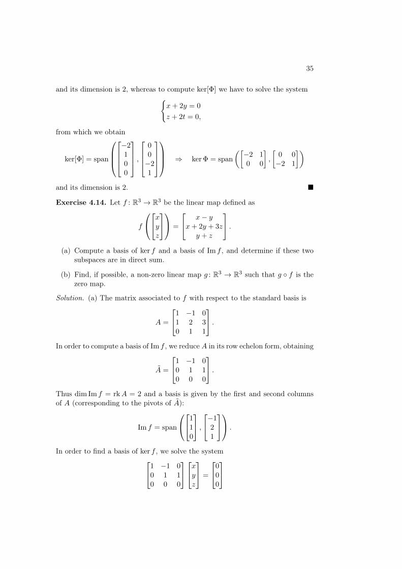
35

and its dimension is 2, whereas to compute ker[Φ] we have to solve the system{x+ 2y = 0

z + 2t = 0,

from which we obtain

ker[Φ] = span

−2100

,

00−21

⇒ ker Φ = span

([−2 10 0

],

[0 0−2 1

])

and its dimension is 2. �

Exercise 4.14. Let f : R3 → R3 be the linear map defined as

f

xyz

=

x− yx+ 2y + 3z

y + z

.(a) Compute a basis of ker f and a basis of Im f , and determine if these two

subspaces are in direct sum.

(b) Find, if possible, a non-zero linear map g : R3 → R3 such that g ◦ f is thezero map.

Solution. (a) The matrix associated to f with respect to the standard basis is

A =

1 −1 01 2 30 1 1

.In order to compute a basis of Im f , we reduce A in its row echelon form, obtaining

A =

1 −1 00 1 10 0 0

.Thus dim Im f = rkA = 2 and a basis is given by the first and second columnsof A (corresponding to the pivots of A):

Im f = span

110

,−1

21

.

In order to find a basis of ker f , we solve the system1 −1 00 1 10 0 0

xyz

=

000


whose set of solutions is

ker f =

−λ−λλ

∣∣∣∣∣∣ λ ∈ R

= span

−1−11

.

The two subspaces ker f and Im f are in direct sum if and only if ker f ∩ Im f ={0}, which is equivalent to ker f * Im f (because dim ker f = 1). Therefore

ker f ∩ Im f = {0} if and only if

−1−11

/∈ Im f.

We know that

−1−11

∈ Im f if and only if there exist a, b ∈ R such that

a

110

+ b

−121

=

−1−11

,that is to say, the system

a− b = −1

a+ 2b = −1

b = 1

has a solution. But it is easy to see that the first two equations are incompatible,thus ker f and Im f are in direct sum.(b) In order to define a linear map, it is sufficient to say what the images of thevectors of a basis are; the image of a generic vector is then uniquely determinedby linearity. We choose the basis B = (v1, v2, v3), where

v1 =

110

, v2 =

−121

, v3 =

−1−11

i.e. (v1, v2) is a basis of Im f and (v3) is a basis of ker f . Notice that B is a basisof the whole space R3 because in (a) we proved that R3 = Im f ⊕ker f . The mapg defined as

g(v1) = 0, g(v2) = 0, g(v3) = v3

is not the zero map, but g(w) = 0 for any w ∈ Im f , therefore (g ◦ f)(v) =g(f(v)) = 0 for any v ∈ R3, i.e. g ◦ f is the zero map. �

Exercise 4.15. Let T : Q[x]≤3 → Q3 be the linear map given by

T (ax3 + bx2 + cx+ d) =

a+ bc+ d

a+ b+ c+ d

.

37

(a) Compute a basis of kerT and a basis of ImT .

(b) Define a linear map F : Q3 → Q[x]≤3 such that kerT ⊕ ImF = Q[x]≤3, ifsuch a map exists.

Solution. (a) We choose the basis (x3, x2, x, 1) for Q[x]≤3 and the standard basisfor Q3. With respect to these two bases, the matrix [T ] associated to T is1 1 0 0

0 0 1 11 1 1 1

.Since ImT is the span of the columns of [T ], the two linearly independent columns1

01

and

011

form a basis of ImT .

In order to compute kerT , we reduce [T ] to the row echelon form, obtaining1 1 0 00 0 1 10 0 0 0

.Therefore a polynomial ax3 + bx2 + cx+ d belongs to kerT if and only if{

a+ b = 0

c+ d = 0.

We can choose (for example) b and d freely, and the other coefficients are forcedto be a = −b and c = −d. So a polynomial belongs to kerT if and only if itscoefficients have the form (−b, b,−d, d) for some b, d ∈ Q, which we may write as

b

−1100

+ d

00−11

.The polynomials corresponding to these two vectors, i.e. −x3 + x2 and −x + 1,form a basis of kerT .(b) In order to answer the question, at first we find a subspace V ⊆ Q[x]≤3 suchthat kerT ⊕ V = Q[x]≤3, then we define a linear function F : Q3 → Q[x]≤3 suchthat ImF = V .

Having fixed a basis, we may think of Q[x]≤3 as Q4, exchanging a polynomialwith the 4-tuple of its coefficients. For answer (a), we saw that

kerT = span

−1100

,

00−11


(more precisely, it is the span of the polynomials that have these 4-tuples ascoefficients). We only have to find other two linearly independent vectors of Q4

such that these four vectors form a basis of Q4. One possible choice is1000

and

0001

,corresponding to polynomials x3 and 1 respectively. So, we may define V =span(x3, 1). Now, if (e1, e2, e3) is the standard basis of Q3, the function F : Q3 →Q[x]≤3 such that F (e1) = x3, F (e2) = 1, F (e3) = 0 (and extended by linearity)satisfies the required conditions. �

Exercise 4.16. Let L : Q4 → Q[x]≤3 the linear map defined by

L

abcd

= (a+ b)x3 + (c+ d)x2 + 2cx+ 2d.

(a) Find a basis of kerL and a basis of ImL.

(b) Determine if exists a linear map G : Q[x]≤3 → Q4 such that kerG = ImLand ImG = kerL.

Chapter 5

Eigenvalues and Eigenvectors

Exercise 5.1. Let M be a 2× 2 matrix with real coefficients and eigenvalues 3

and 5, with eigenvectors[13

]and

[2−6

]respectively.

(a) Compute M[22

].

(b) Find a diagonal matrix D and two matrices A, A−1 (each inverse of theother) such that M = ADA−1.

Exercise 5.2. Let M ∈M3(R) be the matrix

M =

−2 0 1−2 0 1−4 0 2

.Compute the eigenvalues and the eigenvectors of M . Is M diagonalizable?

Solution. The characteristic polynomial is

pM (λ) = det

−2− λ 0 1−2 −λ 1−4 0 2− λ

= −λ3

(use Laplace expansion on the second column), so the only eigenvalue is 0 withalgebraic multiplicity m0 = 3. Let us compute its geometric multiplicity:

ker(M − 0 · I) = kerM = ker

−2 0 1−2 0 1−4 0 2

= ker

−2 0 10 0 00 0 0

.If we use x2 and x3 as free variables, we obtain

kerM =

x3/2x2x3

∣∣∣∣∣∣ x2, x3 ∈ R

= span

1/201

,0

10

39

40 CHAPTER 5. EIGENVALUES AND EIGENVECTORS

and that is also a basis of kerM . It follows that g0 = dim kerM = 2 and M isnot diagonalizable. Moreover, since 0 is the only eigenvalue, the eigenvectors ofM are all and only the vectors of kerM . �

Exercise 5.3. Let M ∈M3(R) be the matrix

M =

−2 2 2−1 1 1−1 1 1

.Compute the eigenvalues and the eigenvectors of M . Is M diagonalizable?

Solution. The characteristic polynomial of M is

pM (λ) = det

−2− λ 2 2−1 1− λ 1−1 1 1− λ

= −λ3.

The only eigenvalue is 0 with algebraic multiplicity m0 = 3. We compute therelative eigenspace:

V0 = kerM = ker

−2 2 2−1 1 1−1 1 1

= ker

−2 2 20 0 00 0 0

.We let y and z be the free variables and, from the first equation of the last system,deduce x = y + z. Therefore

V0 =

y + z

yz

∣∣∣∣∣∣ y, z ∈ R

= span

110

,1

01

.

The non-zero vectors in V0 are the eigenvectors of M . Since g0 = dimV0 = 2 6=m0, M is not diagonalizable. �

Exercise 5.4. Find a basis of R3 made of eigenvectors for the linear map L : R3 →R3 that is represented by the matrix

[L] =

2 1 11 2 11 1 2


Solution. The characteristic polynomial of L is

pL(λ) = det

2− λ 1 11 2− λ 11 1 2− λ

= (2− λ)3 + 1 + 1− 3(2− λ) =

= −λ3 + 6λ2 − 9λ+ 4.

41

We notice that λ = 1 is a solution and proceed with the polynomial division:

−λ3 + 6λ2 − 9λ+ 4

λ− 1= −λ2 + 5λ− 4 = (λ− 1)(4− λ).

Therefore the eigenvalues of L are 1, with algebraic multiplicity m1 = 2, and 4,with algebraic multiplicity m4 = 2. Now we look for eigenvectors.

• For λ = 1, we have

ker([L]− I) = ker

1 1 11 1 11 1 1

= ker

1 1 10 0 00 0 0

=

=

−y − zy

z

∣∣∣∣∣∣ y, z ∈ R

= span

−110

,−1

01

.

• For λ = 4, we have

ker([L]− 4I) = ker

−2 1 11 −2 11 1 −2

.We row-reduce the matrix:

1 1 −20 −3 30 0 0

1 1 −20 −3 30 3 −3

1 1 −21 −2 1−2 1 1

−2 1 11 −2 11 1 −2

permute rows

(second row)− (first row)(third row) + 2(first row)

(third row) + (second row)


If we keep z as a free variable, from the second equation we get y = z andthen substituting into the first one we obtain x + z − 2z = 0 i.e. x = z.Therefore

ker([L]− 4I) =

zzz

∣∣∣∣∣∣ z ∈ R

= span

111

.

The vectors −110

,−1

01

,1

11

are linearly independent and form a basis of R3 made of eigenvectors for L. �

Exercise 5.5. Let T : R3 → R3 be the endomorphism associated to the matrix9 6 93 12 93 6 15

with respect to the standard basis. Say if T is diagonalizable and, if so, computea basis of R3 made of eigenvectors for T .

Solution. In order to simplify the computation, we will work with the matrix

A =1

3[T ] =

3 2 31 4 31 2 5

,remembering that A is diagonalizable if and only if [T ] is diagonalizable. More-over, if λ is an eigenvalue for [T ] with eigenvector v, then λ/3 is an eigenvalue forA with the same eigenvector.

The characteristic polynomial of A is

pA(λ) = det

3− λ 2 31 4− λ 31 2 5− λ

= −λ3 + 12λ2 − 36λ+ 32,

which has roots 2 and 8 with multiplicities m2 = 2 and m8 = 1 respectively.To check if A is diagonalizable we have to compute the geometric multiplicityg2 of the eigenvalue 2 (we already know that the geometric multiplicity of 8 isg8 = m8 = 1, because 1 ≤ g8 ≤ m8 = 1). We have

A− 2I =

1 2 31 2 31 2 3

43

that has rank 1, hence g2 = dim ker(A− 2I) = 2 which is equal to m2. ThereforeA is diagonalizable, and so [T ] is diagonalizable. Let us find the eigenvectors: forthe eigenvalue 2, we have to solve1 2 3

1 2 31 2 3

xyz

=

000

,that is to say x+ 2y + 3z = 0. We can let y, z be free variables and obtain

ker(A− 2I) =

−2y − 3z

yz

∣∣∣∣∣∣ y, z ∈ R

= span

−210

,−3

01

.

Now we have to compute ker(A− 8I), i.e. we have to solve−5 2 31 −4 31 2 −3

xyz

=

000

.After a little computation we obtain

ker(A− 8I) =

zzz

∣∣∣∣∣∣ z ∈ R

= span

111

.

In conclusion a basis of R3 made of eigenvectors of T is

B =

−210

,−3

01

,1

11

.

The matrix associated to T with respect to B is

[T ]BB =

6 0 00 6 00 0 24

. �

Exercise 5.6. Let

M =

0 2 12 3 21 2 0

∈M3(R).

(a) Determine the eigenvalues and the eigenvectors of M over the field R.

(b) Say, justifying the answer, if there exist a matrix V ∈M3(R) and a diagonalmatrix D ∈M3(R) such that M = V DV −1.

(c) Determine a possible choice of such V and D.


Solution. (a) The characteristic polynomial of M is

pM (λ) = det

−λ 2 12 3− λ 21 2 −λ

= −λ3 + 3λ2 + 9λ+ 5 = (−1− λ)2(5− λ).

The eigenvalues of M are the roots of pM (λ), i.e. −1 and 5. Let us find theeigenvectors. The eigenspace relative to −1 is

V−1 = ker(M + I) = ker

1 2 12 4 21 2 1

= ker

1 2 10 0 00 0 0

and a quick computation gives

V−1 = span

−210

,−1

01

.

The eigenspace relative to 5 is

V5 = ker(M − 5I) = ker

−5 2 12 −2 21 2 −5

= ker

1 0 −10 1 −20 0 0

where we row-reduced the matrixM−5I as usual. The solutions of the associatedsystem are

V5 = span

121

.

(b) From answer (a) we have that m−1 = g−1 = 2 and m5 = g5 = 1, so M isdiagonalizable and the matrices V and D do exist. (Otherwise, notice that M issymmetric, thus diagonalizable.)(c) The matrices V and D are respectively the matrix of the eigenvectors and thematrix of the eigenvalues of M : if we put

V =

−2 −1 11 0 20 1 1

and D =

−1 0 00 −1 00 0 5

,it is easy to show that M = V DV −1. �

Exercise 5.7. Let A be the matrix

A =

2 1 0−1 2 00 0 1

.

45

(a) Find the eigenvalues and the eigenvectors of A over the field R. Is A diag-onalizable?

(b) Find the eigenvalues and the eigenvectors of A over the field C. Is A diag-onalizable?

(c) Find an invertible matrix V ∈M3(C) such that V −1AV is diagonal.

Solution. (a) The characteristic polynomial of A is

pA(λ) = det

2− λ 1 0−1 2− λ 00 0 1− λ

= (1− λ)((2− λ)2 + 1

).

Over the field R, the only eigenvalue is λ = 1, because (2 − λ)2 + 1 > 0 for allλ ∈ R, so that polynomial has no roots in R. It follows immediately that A isnot diagonalizable over R, since not all the roots of pA belong to R.

The eigenspace associated to the eigenvalue 1 is

V1 = ker(A− I) = ker

1 1 0−1 1 00 0 0

= ker

1 1 00 2 00 0 0

which is span

001

.

(b) The real eigenvalue and the relative eigenvectors found in (a) are still presentin the complex case. We have to add the roots of (2− λ)2 + 1, that are

2− λ = ±i λ = 2∓ i.

Since the three eigenvalues are different, we conclude that A is diagonalizableover C.

• The eigenspace relative to the eigenvalue 2 + i is

V2+i = ker(A− (2 + i)I) = ker

−i 1 0−1 −i 00 0 −1− i

(?)= ker

−i 1 00 0 00 0 −1− i

where in (?) we added the first row multiplied by i to the second. Thesystem associated to the last matrix is{

−ix+ y = 0

(−1− i)z = 0

and, if x is a free variable, we have

V2+i =

xix

0

∣∣∣∣∣∣ x ∈ C

= span

1i0

.


• The eigenspace relative to the eigenvalue 2− i is

V2−i = ker(A− (2− i)I) = ker

i 1 0−1 i 00 0 −1 + i

(?)= ker

i 1 00 0 00 0 −1 + i

where in (?) we added the first row multiplied by −i to the second. Thesystem associated to the last matrix is{

ix+ y = 0

(−1 + i)z = 0

and, if x is a free variable, we have

V2−i =

x−ix

0

∣∣∣∣∣∣ x ∈ C

= span

1−i0

.

(c) It is sufficient to define V as a matrix that has three linearly independenteigenvectors as columns:

V =

0 1 10 i −i1 0 0

.We know that in this case

V −1AV =

1 0 00 2 + i 00 0 2− i

. �

Exercise 5.8. Let

A =

3 2 31 4 31 2 5

.(a) Is A diagonalizable over R?

(b) Is A diagonalizable over Z3?

Solution. (a) The characteristic polynomial of A is

pA(λ) = det

3− λ 2 31 4− λ 31 2 5− λ

= −λ3 + 12λ2 − 36λ+ 32.

At first we look for rational roots of pA(λ). Recall that, if a polynomial anλn +an−1λ

n−1 + · · ·+a0 with integer coefficients has a rational root p/q (with p and qcoprime), then p divides a0 and q divides an. So, if α is a rational root of pA(λ),

47

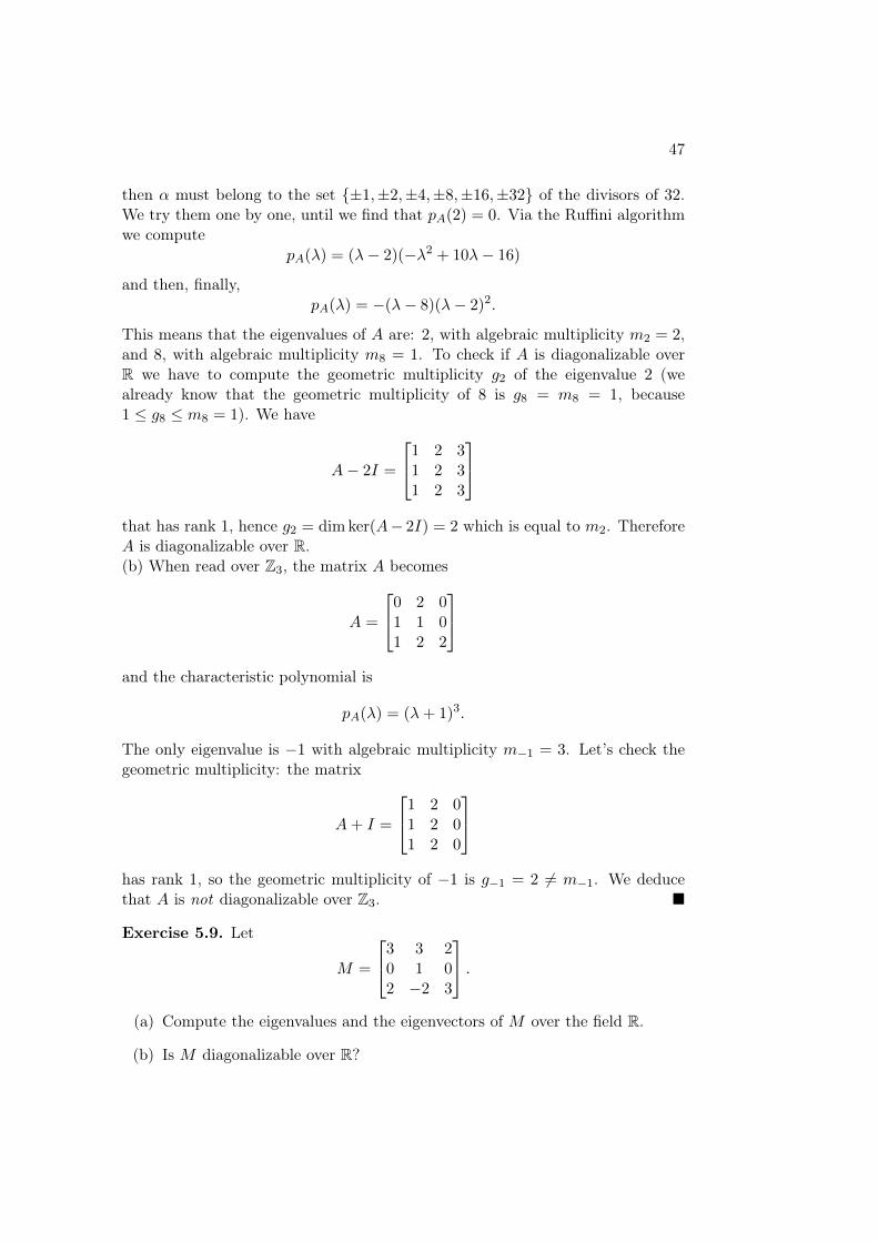
then α must belong to the set {±1,±2,±4,±8,±16,±32} of the divisors of 32.We try them one by one, until we find that pA(2) = 0. Via the Ruffini algorithmwe compute

pA(λ) = (λ− 2)(−λ2 + 10λ− 16)

and then, finally,pA(λ) = −(λ− 8)(λ− 2)2.

This means that the eigenvalues of A are: 2, with algebraic multiplicity m2 = 2,and 8, with algebraic multiplicity m8 = 1. To check if A is diagonalizable overR we have to compute the geometric multiplicity g2 of the eigenvalue 2 (wealready know that the geometric multiplicity of 8 is g8 = m8 = 1, because1 ≤ g8 ≤ m8 = 1). We have

A− 2I =

1 2 31 2 31 2 3

that has rank 1, hence g2 = dim ker(A− 2I) = 2 which is equal to m2. ThereforeA is diagonalizable over R.(b) When read over Z3, the matrix A becomes

A =

0 2 01 1 01 2 2

and the characteristic polynomial is

pA(λ) = (λ+ 1)3.

The only eigenvalue is −1 with algebraic multiplicity m−1 = 3. Let’s check thegeometric multiplicity: the matrix

A+ I =

1 2 01 2 01 2 0

has rank 1, so the geometric multiplicity of −1 is g−1 = 2 6= m−1. We deducethat A is not diagonalizable over Z3. �

Exercise 5.9. Let

M =

3 3 20 1 02 −2 3

.(a) Compute the eigenvalues and the eigenvectors of M over the field R.

(b) Is M diagonalizable over R?


(c) Is M diagonalizable over Z5?

Exercise 5.10. Let K be a field and let T : K4 → K4 be the endomorphismwhose associated matrix (with respect to the standard basis) is

[T ] =

0 0 0 41 0 0 20 1 0 00 0 1 −2

.(a) Compute the characteristic polynomial of T .

(b) Is T diagonalizable for K = R? For K = C? For K = Z5?

Exercise 5.11. Let a ∈ R and consider the matrix

A =

[1 −11 a

].

(a) For which a ∈ R is A diagonalizable over R?

(b) For which a ∈ R is λ = 3 an eigenvalue for A?

(c) For which a ∈ R is v =

[4−1

]an eigenvector for A?

Solution. The characteristic polynomial of A is

pA(λ) = det

[1− λ −1

1 a− λ

]= λ2 − (a+ 1)λ+ (a+ 1).

(a) A is diagonalizable over R if and only if pA(λ) splits through linear factors overR, and the algebraic and geometric multiplicities of the roots are the same. Let usfind the roots: the discriminant of pA(λ) is ∆ = (a+1)2−4(a+1) = (a+1)(a−3),from which we have

λ1 =a+ 1 +

√∆

2and λ2 =

a+ 1−√

∆

2.

• If ∆ > 0, that is a < −1 or a > 3, pA(λ) has two distinct real roots (thathave algebraic multiplicity 1), so A is diagonalizable.

• If ∆ < 0, that is −1 < a < 3, pA(λ) is irreducible over R, so A is notdiagonalizable over R.

• If ∆ = 0, that is a = −1 or a = 3, we have only one eigenvalue λ = (a+1)/2with algebraic multiplicity mλ = 2. We have to compute the geometricmultiplicity.

49

– For a = −1, the eigenvalue is λ = 0 and the matrix becomes

A− λI = A =

[1 −11 −1

],

which clearly has rank 1. Therefore gλ = dim ker(A − λI) = 2 − 1 =1 < mλ and A is not diagonalizable.

– For a = 3, the eigenvalue is λ = 2 and the matrix becomes

A− λI =

[−1 −11 1

]and also in this case its rank is 1, so A is not diagonalizable.

(b) λ = 3 is an eigenvalue for A if and only if it is a root of pA(λ), that is to saypA(3) = 0. But

pA(3) = 32 − (a+ 1) · 3 + (a+ 1) = 7− 2a

and it is 0 if and only if a = 7/2.(c) The vector v is an eigenvector for A if and only if there exists λ ∈ R such thatAv = λv, that is [

1 −11 a

] [4−1

]= λ

[4−1

].

This brings to the system {5 = 4λ

4− a = −λ,

which has a unique solution λ = 5/4 and a = 21/4. Therefore v is an eigenvectorfor A if and only if a = 21/4 (and the relative eigenvalue is λ = 5/4). �

Exercise 5.12. Let k ∈ R and let Bk : R3 → R3 be an endomorphism representedby the matrix

[Bk] =

2 0 0k 1 05 k − 2 1

with respect to the standard basis of R3.

(a) Find the values of k for which the endomorphism Bk is diagonalizable.

(b) Let k = 3. Is it true or false that there exists a basis of R3 such that thematrix associated to B3 with respect to this basis is1 0 3

0 1 40 0 2

?


Solution. (a) The characteristic polynomial of Bk is p(λ) = (2 − λ)(1 − λ)2 forany k. The eigenvalues are λ = 2 with algebraic multiplicity m2 = 1 and λ = 1with algebraic multiplicity m1 = 2. We know that the matrix is diagonalizable ifthese multiplicities are equal to the dimensions of the relative eigenspaces V2 =ker(Bk − 2I) and V1 = ker(Bk − I), where

[Bk]− 2I =

0 0 0k −1 05 k − 2 −1

and [Bk]− I =

1 0 0k 0 05 k − 2 0

.So, we have to compute the dimensions of V2 and V1. A vector with coordinates(a, b, c) belongs to V2 if and only if0 0 0

k −1 05 k − 2 −1

abc

=

000

,that is to say ka− b = 0 and 5a+ (k− 2)b− c = 0. The value of a can be chosenfreely, but after that choice the values of b and c are uniquely determined, sincewe have to put b = ka and c = (k2− 2k+ 5)a. It follows that dimV2 = 1 (i.e. thenumber of free choices), independently from k.

For V1 the computation is similar. A vector (a, b, c) belongs to V1 if and onlyif a = 0, ka = 0 and 5a+ (k − 2)b = 0. The variable c does not appear in theseequations, so its value can be chosen freely. On the other hand a must be 0, sothat (k − 2)b = 0. We have to analyze two cases:

• if k = 2, we can choose freely the value of b, so dimV1 = 2;

• if k 6= 2, we must set b = 0 and the only free choice is that of c, hencedimV1 = 1.

Comparing the dimensions of V2 and V1 with the algebraic multiplicities m2 = 1and m1 = 2, we find that

• if k = 2 the algebraic multiplicities and the geometric ones (i.e. the dimen-sions of the eigenspaces) are the same and Bk is diagonalizable;

• if k 6= 2 we have m1 6= dimV1, so Bk is not diagonalizable.

(b) It is false. To prove this, let L : R3 → R3 be an endomorphism such that thematrix associated to it with respect to some basis B is

[L]B =

1 0 30 1 40 0 2

.We will show that L 6= B3 in any case. In fact, let v1, v2 ∈ R3 be the vectors thathave coordinates respectively (1, 0, 0)B and (0, 1, 0)B with respect to the basis B,

51

and notice that L sends them to themselves, i.e. Lv1 = v1 and Lv2 = v2. (It iseasy to deduce this: look at the first two columns of [L]B. . . ) This implies thatthe dimension of the eigenspace of L relative to the eigenvalue 1, that is to say, thedimension of V1 = {v ∈ R3 | Lv = v}, is at least two, because it contains the twovectors v1 and v2 that are linearly independent. From the previous question, weknow that for k 6= 2, and in particular for k = 3, the dimension of the eigenspaceof B3 relative to the eigenvalue 1 is one, thus L 6= B3.

Alternatively, notice that L is diagonalizable, whereas B3 is not. �

Exercise 5.13. Let S : R3 → R3 be the endomorphism whose associated matrix(with respect to the standard basis) is

[S] =

2 a 11 a+ 1 10 0 1

where a is a real parameter.

(a) For which values of a is S diagonalizable?

(b) For a = −1, find an orthonormal basis of the eigenspace V1 = {v ∈ R3 |S(v) = v} (with respect to the standard inner product on R3).

Exercise 5.14. Let a ∈ R be a real parameter ad let La be the linear endomor-phism of R3 defined as

La

xyz

=

2ax+ y + zx+ ay + z−x+ y + az

.Study the diagonalizability of La, depending on the parameter a.

Solution. The matrix associated to La with respect to the standard basis of R3

is

[La] =

2a 1 11 a 1−1 1 a

and the characteristic polynomial is

pa(λ) = det

2a− λ 1 11 a− λ 1−1 1 a− λ

.If we use the Laplace expansion on the first row we obtain

pa(λ) = (2a− λ)((a− λ)2 − 1

)− (a− λ+ 1) + (1 + a− λ) =

= (2a− λ)(a− λ+ 1)(a+ λ+ 1)


whose roots are all real and given by

λ1 = 2a, λ2 = a− 1, λ3 = a+ 1.

These are the eigenvalues of La; we study what happens if some of these valuesare equal.

First of all, notice that λ2 6= λ3 for every a. If a = 1, then λ1 = λ3 = 2 whichis an eigenvalue with algebraic multiplicity 2; if a = −1, then λ1 = λ2 = −2which is an eigenvalue with algebraic multiplicity 2. So we have to distinguishseveral cases.

• If a 6= ±1, La is diagonalizable since it has three different eigenvalues, eachwith algebraic multiplicity 1.

• If a = 1, we have to compute the geometric multiplicity of the eigenvalue2, i.e. dim ker(L1 − 2I). The associated matrix is

[L1]− 2I =

0 1 11 −1 1−1 1 −1

which has rank 2, so dim ker(L1−2I) = 1 which is different to the algebraicmultiplicity of the eigenvalue 2. It follows that L1 is not diagonalizable.

• The case a = −1 is similar to the previous one: we have to compute thegeometric multiplicity of the eigenvalue −2, i.e. dim ker(L−1 + 2I). We get

[L−1] + 2I =

0 1 11 1 1−1 1 1

and this matrix also has rank 2. Thus the algebraic and geometric mul-tiplicities of the eigenvalue −2 are different and the endomorphism L−1 isnot diagonalizable. �

Exercise 5.15. Let a ∈ R be a real parameter ad let Fa be the linear endomor-phism of R3 that has as associated matrix (with respect to the standard basis)a 0 0

2 1 −a3 −a 1

.Study the diagonalizability of Fa, depending on the parameter a.

Solution. The characteristic polynomial of Fa is

pa(λ) = det

a− λ 0 02 1− λ −a3 −a 1− λ

53

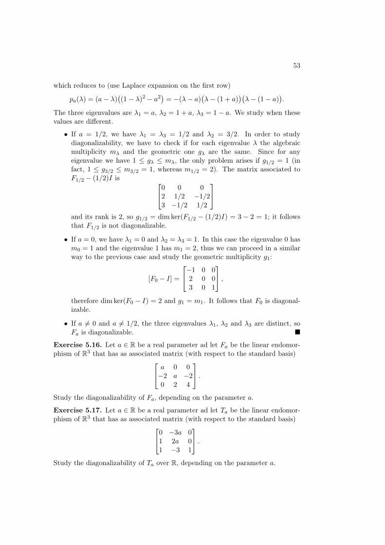
which reduces to (use Laplace expansion on the first row)

pa(λ) = (a− λ)((1− λ)2 − a2

)= −(λ− a)

(λ− (1 + a)

)(λ− (1− a)

).

The three eigenvalues are λ1 = a, λ2 = 1 + a, λ3 = 1− a. We study when thesevalues are different.

• If a = 1/2, we have λ1 = λ3 = 1/2 and λ2 = 3/2. In order to studydiagonalizability, we have to check if for each eigenvalue λ the algebraicmultiplicity mλ and the geometric one gλ are the same. Since for anyeigenvalue we have 1 ≤ gλ ≤ mλ, the only problem arises if g1/2 = 1 (infact, 1 ≤ g3/2 ≤ m3/2 = 1, whereas m1/2 = 2). The matrix associated toF1/2 − (1/2)I is 0 0 0

2 1/2 −1/23 −1/2 1/2

and its rank is 2, so g1/2 = dim ker(F1/2 − (1/2)I) = 3 − 2 = 1; it followsthat F1/2 is not diagonalizable.

• If a = 0, we have λ1 = 0 and λ2 = λ3 = 1. In this case the eigenvalue 0 hasm0 = 1 and the eigenvalue 1 has m1 = 2, thus we can proceed in a similarway to the previous case and study the geometric multiplicity g1:

[F0 − I] =

−1 0 02 0 03 0 1

,therefore dim ker(F0 − I) = 2 and g1 = m1. It follows that F0 is diagonal-izable.

• If a 6= 0 and a 6= 1/2, the three eigenvalues λ1, λ2 and λ3 are distinct, soFa is diagonalizable. �

Exercise 5.16. Let a ∈ R be a real parameter ad let Fa be the linear endomor-phism of R3 that has as associated matrix (with respect to the standard basis) a 0 0

−2 a −20 2 4

.Study the diagonalizability of Fa, depending on the parameter a.

Exercise 5.17. Let a ∈ R be a real parameter ad let Ta be the linear endomor-phism of R3 that has as associated matrix (with respect to the standard basis)0 −3a 0

1 2a 01 −3 1

.Study the diagonalizability of Ta over R, depending on the parameter a.


Solution. The characteristic polynomial of Ta is

pa(λ) = det

−λ −3a 01 2a− λ 01 −3 1− λ

= (1− λ)(λ2 − 2aλ+ 3a)

obtained by using Laplace expansion on the third column. The (reduced) dis-criminant of λ2 − 2aλ + 3a is ∆ = a2 − 3a = a(a− 3), therefore the eigenvaluesof Ta are all real if and only if a ≤ 0 or a ≥ 3, and in this case we have λ1 = 1,λ2 = a+

√∆ and λ3 = a−

√∆.

If a = 0 or a = 3 we have λ2 = λ3 = a; we study for which other values of awe have an eigenvalue with algebraic multiplicity greater than one.

• If a < 0, we test whether λ1 = λ2 (notice that λ1 6= λ3 in this case, sincea < 0 implies λ3 < 0). We get

1 = a+√a2 − 3a ⇒ 1− a =

√a2 − 3a

and, since both sides are positive, we can square:

(1− a)2 = a2 − 3a

that is true for a = −1.

• If a > 3, we have λ2 > 3, so we only have to check if λ1 = λ3 can happen.We get

1 = a−√a2 − 3a ⇒

√a2 − 3a = a− 1

and we can square as above:

a2 − 3a = (a− 1)2

that is true for a = −1, but this can’t be because we are studying the casea > 3.

We reach a first conclusion: if 0 < a < 3, Ta is not diagonalizable because not alleigenvalues are real; if a < 0 and a 6= −1, or a > 3, Ta is diagonalizable becausethe eigenvalues are real and distinct. The only remaining cases are the ones witha double eigenvalue, i.e. a = −1, a = 0 and a = 3.

• If a = −1, the eigenvalue 1 has algebraic multiplicity m1 = 2. We computethe geometric one:

g1 = dim ker(T−1 − I) = dim ker

−1 3 01 −3 01 −3 0

= 2

so T−1 is diagonalizable.

55

• If a = 0, the eigenvalue 0 has algebraic multiplicity m0 = 2. We computethe geometric one:

g0 = dim ker(T0) = dim ker

0 0 01 0 01 −3 1

= 1

so m0 > g0 and T0 is not diagonalizable.

• If a = 3, the eigenvalue 3 has algebraic multiplicity m3 = 2. We computethe geometric one:

g3 = dim ker(T3 − 3I) = dim ker

−3 −9 01 3 01 −3 2

= 1

so m3 > g3 and T3 is not diagonalizable. �

Exercise 5.18. Let a ∈ R be a real parameter ad let Ta be the linear endomor-phism of R3 that has as associated matrix (with respect to the standard basis) 1 0 1

0 a 0a2 0 1

.Study the diagonalizability of Ta over R, depending on the parameter a.

Solution. The characteristic polynomial of Ta is

pa(λ) = det([Ta]− λI) = det

1− λ 0 10 a− λ 0a2 0 1− λ

=

= −(λ− a)(λ− 1 + a)(λ− a− 1),

therefore the eigenvalues of Ta are λ1 = a, λ2 = 1− a and λ3 = 1 + a. We haveto study when these values coincide. Notice that λ1 6= λ3 for all a, so only thefollowing cases are possible:

• λ1 = λ2 if and only if a = 1− a, that is a = 1/2;

• λ2 = λ3 if and only if 1− a = 1 + a, that is a = 0.

So, if a 6= 0 and a 6= 1/2, Ta has three distinct real eigenvalues and it is diago-nalizable. Let us consider now the other cases.

• If a = 0, the eigenvalue 1 has algebraic multiplicity m1 = 2. We computeits geometric multiplicity:

g1 = dim ker([T0]− I) = dim ker

0 0 10 −1 00 0 0

= 1

because the rank of [T0]− I is 2 (the second and third columns are linearlyindependent). Therefore g1 6= m1 and T0 is not diagonalizable.


• If a = 1/2, the eigenvalue 1/2 has algebraic multiplicity m1/2 = 2. Wecompute its geometric multiplicity:

g1/2 = dim ker

([T1/2]−

1

2I

)= dim ker

1/2 0 10 0 0

1/4 0 1/2

=

= dim ker

1/2 0 10 0 00 0 0

= 2.

In this case m1/2 = g1/2 = 2 and T1/2 is diagonalizable. �

Exercise 5.19. Let Ta : R3 → R3 an endomorphism represented by the matrix

[Ta] =

0 2a a0 a+ 2 0a −2 a2 − 1


(a) Determine the values of a ∈ R for which Ta is diagonalizable.

(b) Determine the values of a ∈ R for which Ta is invertible.

Exercise 5.20. Let A ∈M4(R) be the matrix

A =

0 1 0 00 0 −a2 00 0 0 11 0 a2 + 1 0

.Study the diagonalizability of A over the field R depending on the parametera ∈ R.

Solution. The characteristic polynomial of A is

pA(λ) = det(A− λI) = det

−λ 1 0 00 −λ −a2 00 0 −λ 11 0 a2 + 1 −λ

=

= −λ det

−λ −a2 00 −λ 10 a2 + 1 −λ

− 1 det

0 −a2 00 −λ 11 a2 + 1 −λ

=

= −λ(−λ3 − (−λ)(a2 + 1))− (−a2) =

= λ4 − (a2 + 1)λ2 + a2

57

where we used the Laplace expansion on the first row (other choices are possible).In order to find its roots we put λ2 = t and we get the quadratic equation

t2 − (a2 + 1)t+ a2 = 0,

whose solutions are t1 = 1 and t2 = a2. Therefore the solutions of pA(λ) = 0 aregiven by λ = ±

√t1 and λ = ±

√t2, i.e.

λ1 = 1, λ2 = −1, λ3 = a, λ4 = −a.

These solutions are always distinct, unless a ∈ {0, 1,−1}. Thus we may concludethat for a /∈ {0, 1,−1} A is diagonalizable, and study the other cases separately.

• If a = 0, the eigenvalues are 1, −1 and 0 with algebraic multiplicitiesm1 = m−1 = 1 and m0 = 2. Since the geometric multiplicity is always lessthan or equal to the algebraic one, the only computation we have to do isthat of g0, the geometric multiplicity of the eigenvalue 0.

dim ker(A− 0I) = dim ker

0 1 0 00 0 0 00 0 0 11 0 1 0

(?)= dim ker

1 0 1 00 1 0 00 0 0 10 0 0 0

= 1

where we performed the usual row-reduction algorithm in (?). Thereforeg0 6= m0 and A is not diagonalizable.

• Notice that the matrix A is the same both for a = 1 and for a = −1, so wecan study these two cases together. The eigenvalues are 1 and −1, each withalgebraic multiplicity m±1 = 2, and we have to compute the two geometricmultiplicities. Let us begin with g1:

dim ker(A− I) = dim ker

−1 1 0 00 −1 −1 00 0 −1 11 0 2 −1

= 1.

From this computation we see that g1 6= m1, so we can immediately con-clude that A is not diagonalizable. �

Exercise 5.21. (I) Let A : C2 → C2 the endomorphism associated to the matrix[1 −22 1

]with respect to the standard basis. Find the eigenvectors of A and determine ifA is diagonalizable.(II) Consider the endomorphism B : R2 → R2 associated to the matrix[

1 bb 1

]with respect to the standard basis, where b ∈ R is a parameter.


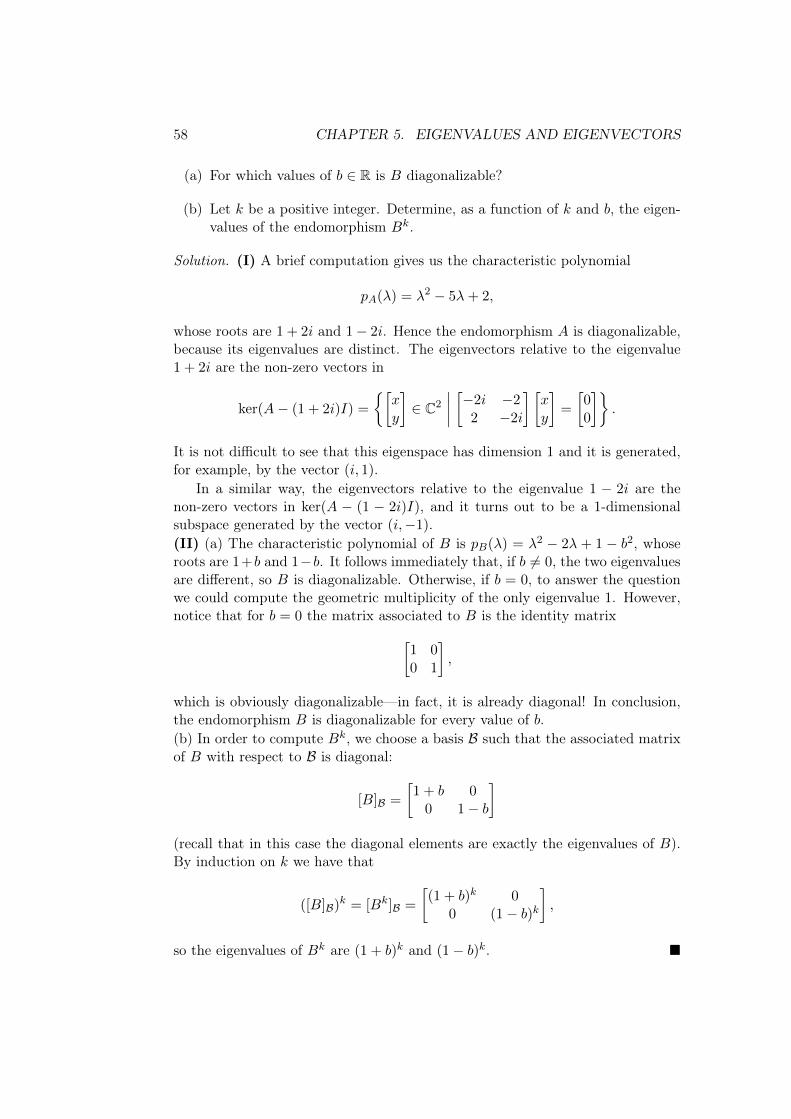
(a) For which values of b ∈ R is B diagonalizable?

(b) Let k be a positive integer. Determine, as a function of k and b, the eigen-values of the endomorphism Bk.

Solution. (I) A brief computation gives us the characteristic polynomial

pA(λ) = λ2 − 5λ+ 2,

whose roots are 1 + 2i and 1− 2i. Hence the endomorphism A is diagonalizable,because its eigenvalues are distinct. The eigenvectors relative to the eigenvalue1 + 2i are the non-zero vectors in

ker(A− (1 + 2i)I) =

{[xy

]∈ C2

∣∣∣∣ [−2i −22 −2i

] [xy

]=

[00

]}.

It is not difficult to see that this eigenspace has dimension 1 and it is generated,for example, by the vector (i, 1).

In a similar way, the eigenvectors relative to the eigenvalue 1 − 2i are thenon-zero vectors in ker(A − (1 − 2i)I), and it turns out to be a 1-dimensionalsubspace generated by the vector (i,−1).(II) (a) The characteristic polynomial of B is pB(λ) = λ2 − 2λ + 1 − b2, whoseroots are 1+b and 1−b. It follows immediately that, if b 6= 0, the two eigenvaluesare different, so B is diagonalizable. Otherwise, if b = 0, to answer the questionwe could compute the geometric multiplicity of the only eigenvalue 1. However,notice that for b = 0 the matrix associated to B is the identity matrix[

1 00 1

],

which is obviously diagonalizable—in fact, it is already diagonal! In conclusion,the endomorphism B is diagonalizable for every value of b.(b) In order to compute Bk, we choose a basis B such that the associated matrixof B with respect to B is diagonal:

[B]B =

[1 + b 0

0 1− b

](recall that in this case the diagonal elements are exactly the eigenvalues of B).By induction on k we have that

([B]B)k = [Bk]B =

[(1 + b)k 0

0 (1− b)k],

so the eigenvalues of Bk are (1 + b)k and (1− b)k. �

59

Exercise 5.22. Let B be the matrix2 1 1 11 2 1 11 1 2 11 1 1 2

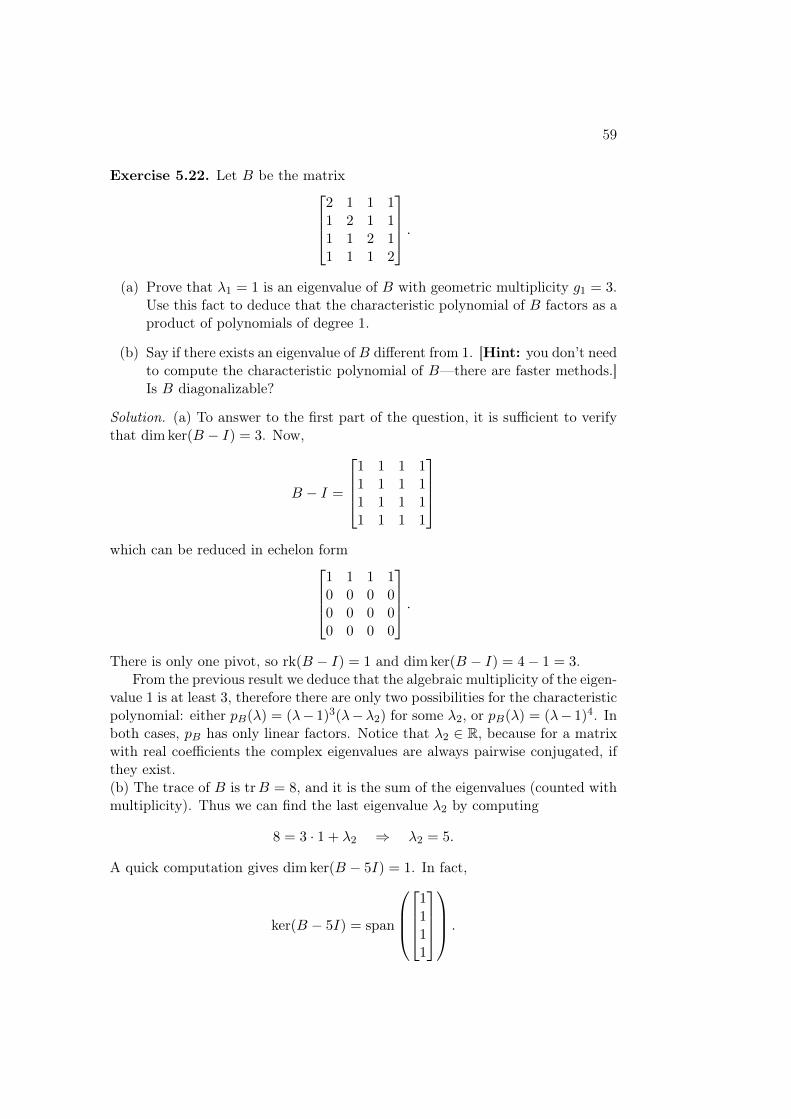
.(a) Prove that λ1 = 1 is an eigenvalue of B with geometric multiplicity g1 = 3.

Use this fact to deduce that the characteristic polynomial of B factors as aproduct of polynomials of degree 1.

(b) Say if there exists an eigenvalue of B different from 1. [Hint: you don’t needto compute the characteristic polynomial of B—there are faster methods.]Is B diagonalizable?

Solution. (a) To answer to the first part of the question, it is sufficient to verifythat dim ker(B − I) = 3. Now,

B − I =

1 1 1 11 1 1 11 1 1 11 1 1 1

which can be reduced in echelon form

1 1 1 10 0 0 00 0 0 00 0 0 0

.There is only one pivot, so rk(B − I) = 1 and dim ker(B − I) = 4− 1 = 3.

From the previous result we deduce that the algebraic multiplicity of the eigen-value 1 is at least 3, therefore there are only two possibilities for the characteristicpolynomial: either pB(λ) = (λ− 1)3(λ−λ2) for some λ2, or pB(λ) = (λ− 1)4. Inboth cases, pB has only linear factors. Notice that λ2 ∈ R, because for a matrixwith real coefficients the complex eigenvalues are always pairwise conjugated, ifthey exist.(b) The trace of B is trB = 8, and it is the sum of the eigenvalues (counted withmultiplicity). Thus we can find the last eigenvalue λ2 by computing

8 = 3 · 1 + λ2 ⇒ λ2 = 5.

A quick computation gives dim ker(B − 5I) = 1. In fact,

ker(B − 5I) = span

1111

.


In conclusion, since m1 = g1 = 3 and m5 = g5 = 1, B is diagonalizable.Otherwise, we can say immediately that B is diagonalizable because it is

symmetric. �

Chapter 6

Scalar Products

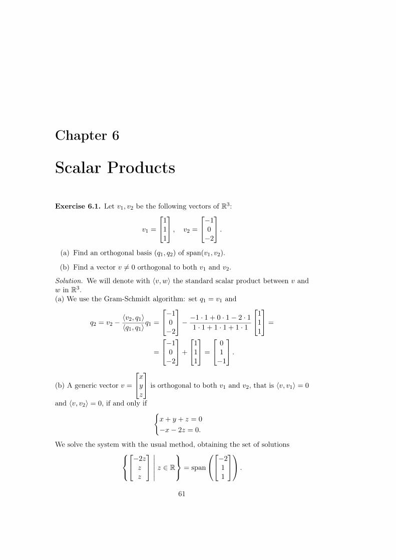
Exercise 6.1. Let v1, v2 be the following vectors of R3:

v1 =

111

, v2 =

−10−2

.(a) Find an orthogonal basis (q1, q2) of span(v1, v2).

(b) Find a vector v 6= 0 orthogonal to both v1 and v2.

Solution. We will denote with 〈v, w〉 the standard scalar product between v andw in R3.(a) We use the Gram-Schmidt algorithm: set q1 = v1 and

q2 = v2 −〈v2, q1〉〈q1, q1〉

q1 =

−10−2

− −1 · 1 + 0 · 1− 2 · 11 · 1 + 1 · 1 + 1 · 1

111

=

=

−10−2

+

111

=

01−1

.(b) A generic vector v =

xyz

is orthogonal to both v1 and v2, that is 〈v, v1〉 = 0

and 〈v, v2〉 = 0, if and only if {x+ y + z = 0

−x− 2z = 0.

We solve the system with the usual method, obtaining the set of solutions−2z

zz

∣∣∣∣∣∣ z ∈ R

= span

−211

.

61

62 CHAPTER 6. SCALAR PRODUCTS

Any non-zero vector in this set (e.g. v =

−211

) answers the question.

Alternatively, we could proceed with Gram-Schmidt: take any vector v3 /∈span(v1, v2) and set

v = v3 −〈v3, q1〉〈q1, q1〉

q1 −〈v3, q2〉〈q2, q2〉

q2. �

Chapter 7

More Exercises

Exercise 7.1. (I) Determine the coordinates of the vector

v =

23−3

with respect to the basis B = (v1, v2, v3) of R3, where

v1 =

1−10

, v2 =

101

, v3 =

−111

.(II) Let f : R3 → R3 be the linear map whose associated matrix with respect tothe basis B is

A = [f ]B =

2 −1 0−1 −2 21 −1 3

.Determine the coordinates of f(v) with respect to the standard basis of R3.

Solution. (I) The coordinates of v are the coefficients of the linear combination 23−3

= x

1−10

+ y

101

+ z

−111

,which are found by solving the system 1 1 −1

−1 0 10 1 1

xyz

=

23−3

.We represent the system with the matrix 1 1 −1 2

−1 0 1 30 1 1 −3

.63

64 CHAPTER 7. MORE EXERCISES

By elementary row operations we don’t change the set of solutions; after a bit ofcomputation we get the row reduced echelon form1 0 0 −11

0 1 0 50 0 1 −8

,so the coordinates of v with respect to B are (−11, 5,−8).(II) Since A represents f with respect to the basis B and now we know the coor-dinates of v with respect to the same basis, it is easy to compute the coordinatesof f(v) with respect to B:

[f(v)]B = [f ]B[v]B =

2 −1 0−1 −2 21 −1 3

−115−8

=

−27−15−40

.This means that f(v) = −27v1 − 15v2 − 40v3. We already know the coordinatesof v1, v2, v3 with respect to the standard basis, so we can conclude

f(v) = −27

1−10

− 15

101

− 40

−111

=

−2−13−55

. �

Exercise 7.2. Let f : R3 → R3 be the linear map given by

f

xyz

=

z + yy + x

2x

.(a) Compute the matrix A = [f ] associated to f with respect to the standard

basis of R3.

(b) Compute the matrix M = [f ]BB associated to f with respect to the basisB = (v1, v2, v3), where

v1 =

111

, v2 =

210

, v3 =

−100

.(c) Compute one eigenvalue of f .

Solution. In general, recall that if g : V →W is a linear map and V,W are basesrespectively of V and W , the matrix [g]WV associated to g has in the i-th columnthe coordinates of g(vi) with respect to the basis W, where vi is the i-th vectorof V.(a) If C = (e1, e2, e3) is the standard basis, we compute

65

• f(e1) = f

100

=

012

;

• f(e2) = f

010

=

110

;

• f(e3) = f

001

=

100

;therefore

A =

0 1 11 1 02 0 0

.(b) We have to compute f(vi) for i = 1, 2, 3.

• f(v1) = f

111

=

222

and we easily see that f(v1) = 2v1 + 0v2 + 0v3,

so the first column of M is

200

.

• f(v2) = f

210

=

134

and the coordinates with respect to B are not

computed as easily as the previous point. We have to find a, b, c ∈ R suchthat av1 + bv2 + cv3 = f(v2), i.e. we have to solve the system1 2 −1

1 1 01 0 0

abc

=

134

.The computation is not difficult and it turns out that f(v2) = 4v1−v2 +v3.

• f(v3) = f(−e1) = −f(e1) =

0−1−2

.With a computation like the one above,

we obtain f(v3) = −2v1 + v2 + 0v3.

Therefore

M =

2 4 −20 −1 10 1 0

.


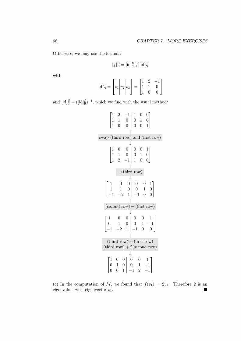
Otherwise, we may use the formula

[f ]BB = [id]BC [f ][id]CB

with

[id]CB =

v1∣∣∣∣∣∣v2∣∣∣∣∣∣v3 =

1 2 −11 1 01 0 0

and [id]BC = ([id]CB)−1, which we find with the usual method:

1 0 00 1 00 0 1

∣∣∣∣∣∣0 0 10 1 −1−1 2 −1

1 0 00 1 0−1 −2 1

∣∣∣∣∣∣0 0 10 1 −1−1 0 0

1 0 01 1 0−1 −2 1

∣∣∣∣∣∣0 0 10 1 0−1 0 0

1 0 01 1 01 2 −1

∣∣∣∣∣∣0 0 10 1 01 0 0

1 2 −11 1 01 0 0

∣∣∣∣∣∣1 0 00 1 00 0 1

swap (third row) and (first row)

−(third row)

(second row)− (first row)

(third row) + (first row)(third row) + 2(second row)

(c) In the computation of M , we found that f(v1) = 2v1. Therefore 2 is aneigenvalue, with eigenvector v1. �

67

Exercise 7.3. Let V ⊆ R4 be the subspace V = span(v1, v2), where

v1 =

1110

and v2 =

1310

.(a) Verify that (v1, v2) is a basis of V and extend it to a basis of R4.

(b) Does it exist a linear map T : R4 → R4 such that kerT = ImT = V ? Ifnot, explain why, otherwise choose a basis B of R4 and write the matrix[T ]BB associated to T with respect to this basis.

Solution. (a) We only need to check if v1 and v2 are linearly independent. Werow-reduce the matrix whose columns are v1 and v2:

1 11 31 10 0

1 10 20 00 0

.The pivots are in both columns, so v1 and v2 are indeed linearly independent. Inorder to extend (v1, v2) to a basis of R4, we row-reduce the matrix

1 11 31 10 0

∣∣∣∣∣∣∣∣1 0 0 00 1 0 00 0 1 00 0 0 1

.After a quick computation, the row reduced form is

1 1 1 0 0 00 2 −1 1 0 00 0 −1 0 1 00 0 0 0 0 1

which has pivots in the 1st, 2nd, 3rd and 6th columns. Therefore the set

B =

v1, v2, v3 =

1000

, v4 =

0001

is a basis of R4 that extends (v1, v2).(b) We choose the basis B of point (a). Since we must have kerT = V , we defineT (v1) = 0 and T (v2) = 0. On the other hand

ImT = span(T (v1), T (v2), T (v3), T (v4)) = span(T (v3), T (v4))


and this has to be equal to V = span(v1, v2). The easiest way is to defineT (v3) = v1 and T (v4) = v2. The associated matrix with respect to B is

[T ]BB =

0 0 1 00 0 0 10 0 0 00 0 0 0

.We know for sure that ImT = span(v1, v2) = V and kerT ⊇ span(v1, v2) = V .But dim kerT + dim ImT = 4, so kerT can’t contain V properly. �

Exercise 7.4. Let C be the matrix

C =

1 1 1 10 1 0 11 0 1 0

.(a) Find a basis of U = kerC and a basis of W = ImC.

(b) Find a set of cartesian equations for W , i.e. write W as the set of solutionsof a homogeneous linear system.

Solution. (a) We row-reduce C in echelon form:

C =

1 0 1 00 1 0 10 0 0 0

.The pivots are in the first and second columns of C, so the respective columns ofC form a basis of ImC:

W = span

101

,1

10

.

To find a basis of kerC, we solve the system associated to C:{x+ z = 0

y + t = 0

from which we get

U = kerC =

−z−tzt

∣∣∣∣∣∣∣∣ z, t ∈ R

= span

−1010

,

0−101

.

69

(b) A generic vector with coordinates (x, y, z) belongs to W if and only if thematrix 1 1 x

0 1 y1 0 z

has not maximum rank. Its row reduced echelon form is1 1 x

0 1 y0 0 −x+ y + z

which has not rank 3 if and only if −x+ y + z = 0. Therefore

W =

xyz

∈ R3

∣∣∣∣∣∣ −x+ y + z = 0

. �

Exercise 7.5. Consider the following two subspaces of R3:

V =

xyz

∈ R3

∣∣∣∣∣∣ x+ y + z = 0

and W = span

1−12

.

(a) Compute a basis of V +W and say if they are in direct sum.

(b) Find a linear map f : R3 → R3 such that ker f = V and Im f = W .

(c) Prove that the set

{f : R3 → R3 | f is linear, V ⊆ ker f and Im f ⊆W}

is a linear subspace of the space of all linear endomorphisms of R3.

Exercise 7.6. Let V be the subspace of R[x]≤5 (polynomials with real coefficientsand degree less than or equal to 5) defined as

V = {p(x) ∈ R[x]≤5 | p(1) = p(−1) = 0}.

(a) Determine a basis for V over R.

(b) Determine whether there exist injective or surjective linear maps from V tothe space W of 2× 2 symmetric matrices with real coefficients, and explainwhy.

Solution. A generic 2× 2 symmetric matrix with real coefficients has the form[a bb c

]


with a, b, c ∈ R, so the space W has dimension 3 over R and a basis is given by[1 00 0

],

[0 11 0

],

[0 00 1

].

In order to study the existence of injective or surjective linear maps from V toW , we have to compare their dimensions. In particular,

• there exist injective maps from V to W if and only if dimV ≤ dimW (senda basis of V injectively to a set of linearly independent vectors of W );

• there exist surjective maps from V to W if and only if dimV ≥ dimW(send a basis of V surjectively to a basis of W ).

We have to compute dimV , and to do so we will find a basis of V , thus answering(a) and (b) at the same time.

Recall that α is a root of a polynomial p (i.e. p(α) = 0) if and only if (x− α)is a factor of p(x), that is to say that there exists a polynomial q(x) such thatp(x) = (x − α)q(x). Therefore the condition p(1) = p(−1) = 0 is equivalent tothe fact that (x− 1) and (x+ 1) are factors of p(x). Then, for any p(x) ∈ V wecan find a polynomial q(x) such that

p(x) = (x− 1)(x+ 1)q(x)

and, since deg p = 2+deg q, we have also deg q ≤ 3. It is easy to see that this mapfrom V to the space R[x]≤3 is linear and bijective (given a polynomial q(x) withdeg q ≤ 3, its inverse image is the polynomial (x− 1)(x+ 1)q(x), that belongs toV ), so it is an isomorphism of vector spaces. Now, dim(R[x]≤3) = 4 and a basisis given by {x3, x2, x, 1}, therefore we can conclude that dimV = 4 and a basisfor V is

{(x− 1)(x+ 1)x3, (x− 1)(x+ 1)x2, (x− 1)(x+ 1)x, (x− 1)(x+ 1)}

obtained by taking the inverse images of the vectors in the basis of R[x]≤3.Finally, since dimV is strictly greater than dimW , we can say that there exist

surjective linear maps from V to W but not injective ones. �

Exercise 7.7. Let V = Mn(R) be the vector space of n × n matrices over thefield R. Let S = {M ∈ V | M = MT} be the subspace of symmetric matrices,and let A = {M ∈ V | −M = MT} be subspace of antisymmetric matrices.

(a) Prove that V = S ⊕A.

(b) Let ϕ : V → V the linear map defined as

ϕ(M) = M +MT.

Determine if ϕ is diagonalizable and, if so, compute a basis of V made ofeigenvectors for ϕ.

linear algebra: exercisespeople.dm.unipi.it/berardu/didattica/2016-17mdal/eserciziario... · 10...

Documents