linear algebra ii - group for dynamical systems and approximation
TRANSCRIPT
LINEAR ALGEBRA II
J. B. Cooper
Johannes Kepler Universitat Linz
Contents
1 DETERMINANTS 31.1 Introduction . . . . . . . . . . . . . . . . . . . . . . . . . . . 31.2 Existence of the determinant
and how to calculate it . . . . . . . . . . . . . . . . . . . . . 51.3 Further properties of the determinant . . . . . . . . . . . . . . 101.4 Applications of the determinant . . . . . . . . . . . . . . . . . 20
2 COMPLEXNUMBERS ANDCOMPLEX VECTOR SPACES 262.1 The construction of C . . . . . . . . . . . . . . . . . . . . . . 262.2 Polynomials . . . . . . . . . . . . . . . . . . . . . . . . . . . . 322.3 Complex vector spaces and matrices . . . . . . . . . . . . . . 37
3 EIGENVALUES 403.1 Introduction . . . . . . . . . . . . . . . . . . . . . . . . . . . 403.2 Characteristic polynomials and diagonalisation . . . . . . . . . 443.3 The Jordan canonical form . . . . . . . . . . . . . . . . . . . . 503.4 Functions of matrices and operators . . . . . . . . . . . . . . 633.5 Circulants and geometry . . . . . . . . . . . . . . . . . . . . . 713.6 The group inverse and the Drazin inverse . . . . . . . . . . . 74
4 EUCLIDEAN AND HERMITIAN SPACES 774.1 Euclidean space . . . . . . . . . . . . . . . . . . . . . . . . . 774.2 Orthogonal decompositions . . . . . . . . . . . . . . . . . . . 894.3 Self-ajdoint mappings— the spectral theorem . . . . . . . . . 914.4 Conic sections . . . . . . . . . . . . . . . . . . . . . . . . . . . 984.5 Hermitian spaces . . . . . . . . . . . . . . . . . . . . . . . . . 1004.6 The spectral theorem—complex version . . . . . . . . . . . . . 1034.7 Normal operators . . . . . . . . . . . . . . . . . . . . . . . . . 1074.8 The Moore-Penrose inverse . . . . . . . . . . . . . . . . . . . 112
1

4.9 Positive definite matrices . . . . . . . . . . . . . . . . . . . . 119
5 MULTILINEAR ALGEBRA 1235.1 Dual spaces . . . . . . . . . . . . . . . . . . . . . . . . . . . . 1235.2 Duality in euclidean spaces . . . . . . . . . . . . . . . . . . . 1315.3 Multilinear mappings . . . . . . . . . . . . . . . . . . . . . . 1325.4 Tensors . . . . . . . . . . . . . . . . . . . . . . . . . . . . . . 141
2
1 DETERMINANTS
1.1 Introduction
In this chapter we treat one of the most important themes of linear algebra—that of the determinant. We begin with some remarks which will motivatethe formal definition:I. Recall that the system
ax+ by = e
cx+ dy = f
has the unique solution
x =ed− fb
ad − bcy =
af − ce
ad− bc
provided that the denominator ad − bc is non-zero. If we introduce thenotation
det
[a bc d
]= ad− bc
we can write the solution in the form
x = det
[e bf d
]÷ det
[a bc d
]
y = det
[a ec f
]÷ det
[a bc d
]
(Note that the numerators are formed by replacing the column of the matrix
A =
[a bc d
]
corresponding to the unknown by the column vector on the right hand side).Earlier, we displayed a similar formula for the solution of a system of
three equations in three unknowns. It is therefore natural to ask whetherwe can define a function det on the space Mn of n× n matrices so that thesolution of the equation AX = Y is, under suitable conditions, given by theformula
xi =detAi
detA
3

where Ai is the matrix that we obtain by replacing the i-th column of A byY i.e.
Ai =
a11 a12 . . . a1,i−1 y1 a1,i+1 . . . a1n...
...an1 an2 . . . an,i−1 yn an,i+1 . . . ann
.
II. Recall that
ad− bc = det
[a bc d
]
is the area of the parallelogram spanned by the vectors (a, c) and (b, d). Nowif f is the corresponding linear mapping on R2, this is just the image of thestandard unit square (i.e. the square with vertices (0, 0), (1, 0), (0, 1), (1, 1))under f . The natural generalisation would be to define the determinant ofan n×n matrix to be the n-dimensional volume of the image of the standardhypercube in Rn under the linear mapping induced by the matrix. Althoughwe do not intend to give a rigorous treatment of the volume concept in higherdimensional spaces, it is geometrically clear that it should have the followingproperties:a) the volume of the standard hypercube is 1. This means that the determi-nant of the unit matrix is 1;b) the volume depends linearly on the length of a fixed side. This meansthat the function det is linear in each column i.e.
det[A1 . . . Ai + A′i . . . An] = det[A1 . . . A)i . . . An] + det[A1 . . . A
′i . . . An]
anddet[A1 . . . λAi . . . An] = λ det[A1 . . . An].
c) The volume of a degenerate parallelopiped is zero. This means that if twocolumns of the matrix coincide, then its determinant vanishes.
(Note that the volume referred to here can take on negative values—depending on the orientation of the parallelopiped).
4

1.2 Existence of the determinantand how to calculate it
We shall now proceed to show that a function with the above propertiesexists. In fact it will be more convenient to demand the analogous propertiesfor the rows i.e. we shall construct, for each n, a function
det :Mn → R
with the propertiesd1) det In = 1;d2)
det
A1...
λAi + µA′i
...An
= λ det
A1...Ai...An
+ µ det
A1...A′
i...An
.
d3) if Ai = Aj(i 6= j), then
det
A1...Ai...Aj...An
= 0.
Before we prove the existence of such a function, we shall derive some furtherproperties which are a consequence of d1) - d3):d4) if we add a multiple of one row to another one, the value of the determi-nant remains unaltered i.e.
det
A1...Ai...Aj...An
= det
A1...
Ai + Aj...Aj...An
;
5
d5) if we interchange two rows of a matrix, then we alter the sign of thedeterminant i.e.
det
A1...Ai...Aj...An
= − det
A1...Aj...Ai...An
.
d6) if one row of A is a linear combination of the others, then detA = 0.Hence if r(A) < n (i.e. if A is not invertible), then detA = 0.Proof. d4)
det
A1...
Ai + Aj...Aj...An
= det
A1...Ai...Aj...An
+ det
A1...Aj...Aj...An
= det
A1...Ai...Aj...An
by d3).d5)
det
A1...Ai...Aj...An
= det
A1...
Ai + Aj...Aj...An
det
A1...
Ai + Aj...
−Ai...An
= − det
A1...Aj...Ai...An
.
d6) Suppose that Ai = λ1A1 + · · ·+ λi−1Ai−1. Then
det
A1...
Ai−1
Ai...An
= det
A1...
Ai−1
(λ1A1 + . . . λi−1Ai−1)...An
= 0
6

since if we expand the expression by using the linearity in the i-th row weobtain a sum of multiples of determinants each of which has two identicalrows and these vanish.
Note the fact that with this information we are able to calculate thedeterminant of a given matrix, despite the fact that it has not yet beendefined! We simply reduce the matrix A to Hermitian form A by usingelementary transformations. At each step the above rules tell us the effecton the determinant. If there is a zero on the diagonal of A (i.e. if r(A) < n),then detA = 0 by d6) above. If not, we can continue to reduce the matrix tothe unit matrix by further row operations and so calculate its determinant.In fact, a little reflection shows that most of these calculations are superfluousand that it suffices to reduce the matrix to upper triangular form since thedeterminant of the latter is the product of its diagonal elements.
We illustrate this by “calculating” the determinant of the 3× 3 matrix
0 2 31 2 12 −3 2
.
We have
det
0 2 31 2 12 −3 2
= − det
1 2 10 2 32 −3 2
= − det
1 2 10 2 30 −7 0
= −2 det
1 2 10 1 3
2
0 −7 0
= −2 det
1 2 10 1 3
2
0 0 212
= −21.
In fact, what the above informal argument actually proves is the unique-ness of the determinant function. This fact is often useful and we state it asa Proposition.
Proposition 1 There exists at most one mapping det : Mn → R with theproperties d1)-d3) above.
7

The main result of this section is the fact that such a function does in factexist. The proof uses an induction argument on n. We already know that adeterminant function exists for n = 1, 2, 3. In order to motivate the followingproof note the formula
a11(a22a33 − a32a23)− a21(a12a33 − a32a13) + a31(a12a23 − a22a13)
for the determinant of the 3× 3 matrixa11 a12 a13a21 a22 a23a31 a32 a33
.
This is called the development of the determinant along the first column andsuggests how to extend the definition to one dimension higher. This will becarried out formally in the proof of the following Proposition:
Proposition 2 There is a (and hence exactly one) function det : Mn → Rwith the properties d1)-d3) (and so also d4)-d6)).
Proof. As indicated above, we prove this by induction on n. The casen = 1 is clear (take det[a] = a). The step from n− 1 to n: we define
detA =n∑
i=1
(−1)i+1ai1 detAi1
where Ai1 is the (n−1)×(n−1) matrix obtained by deleting the first columnand the i-throw of A (the induction hypothesis ensures that its determinantis defined) and show that this function satisfies d1), d2) and d3). It is clearthat det In = 1. We verify the linearity in the k-th row as following. Itsuffices to show that each term ai1 detAi1 is linear in the k-th row. Now ifi 6= k a part of the k-th row of A is a row of Ai1 and so this term is linear bythe induction hypothesis. if i = k, then detAi1 is independent of the k-throwand ai1 depends linearly on it.
It now remains to show that detA = 0 whenever two rows of A areidentical, say the k-th and the l-th (with k < l). Consider the sum
n∑
i=1
(−1)i+1ai1 detAi1.
then Ai1 has two identical rows (and so vanishes by the induction hypothesis)except for the cases where j = k or j = l. This leaves the two terms
(−1)k+1ak1 detAk1 and (−1)l+1al1 detAl1
8

and they are equal in absolute value, but with opposite signs. (For ak1 = al1and Ak1 is obtained from Al1 by moving one row (k − l − 1) places. Thiscan be achieved by the same number of row exchanges and so multiplies thedeterminant by (−1)k−l−1).
The above proof yields the formula
detA =
n∑
i=1
(−1)i+1ai1 detAi1
for the determinant which is called the development along the first col-umn. Similarly, one can develop detA along the j-th column i.e. we havethe formula
detA =n∑
i=1
(−1)i+jaij detAij
where Aij is the (n − 1) × (n − 1) matrix obtained from A by omitting thei-th row and the j-th column. This can be proved by repeating the aboveproof with this recursion formula in place of the original one.
Example: If we expand the determinant of the triangular matrix
A =
a11 a12 . . . a1n0 a22 . . . a2n...
...0 0 . . . ann
along the first column, we see that its determinant is
a11 det
a22 . . . a2n0 . . . a3n...
...0 . . . ann
.
An obvious induction argument shows that the determinant is a11a22 . . . ann,the product of the diagonal elements. In particular, this holds for diagonalmatrices.
This provides a justification for the method for calculating the determi-nant of a matrix by reducing it to triangular form by means of elementaryrow operations. Note that for small matrices it is usually more convenientto calculate the determinant directly from the formulae given earlier.
9

1.3 Further properties of the determinant
d7) if r(A) = n i.e. A is invertible, then detA 6= 0.Proof. For then the Hermitian form of A has non-zero diagonal elementsand so the determinant of A is non-zero.
Combining d5) and d7) we have the following Proposition:
Proposition 3 An n×n matrix A is invertible if and only if its determinantis non-zero.
Shortly we shall see how the determinant can be used to give an explicitformula for the inverse.d8) The determinant is multiplicative i.e.
detAB = detA · detB.
Proof. This is a typical application of the uniqueness of the determinantfunction. We first dispose of the case where detB = 0. Then r(B) < n andso r(AB) < n. In this case the formula holds trivially since both sides arezero.
If detB 6= 0, then the mapping
A 7→ detAB
detB
is easily seen to satisfy the three characteristic properties d1)-d3) of thedeterminant function and so is the determinant.d9) Suppose that A is an n× n matrix whose determinant does not vanish.Then, as we have seen, A is invertible and we now show that the inverse ofA can be written down explicitly as follows:
A−1 =1
detA(adjA)
where adjA is the matrix [(−1)i+j detAji]. (i.e. we form the matrix whose(i, j)-th entry is the determinant of the matrix obtained by removing the i-throw and the j-th column of A, with sign according to the chess-board pattern
+ − + − . . .− + − + . . ....
This matrix is then transposed and the result is divided by detA.
10
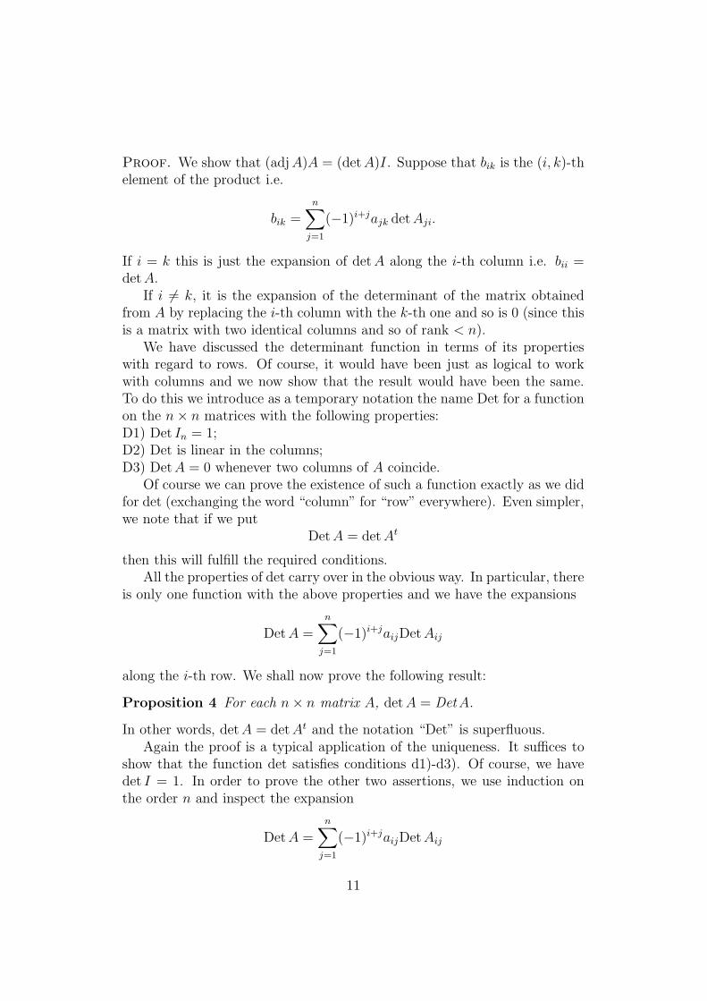
Proof. We show that (adjA)A = (detA)I. Suppose that bik is the (i, k)-thelement of the product i.e.
bik =n∑
j=1
(−1)i+jajk detAji.
If i = k this is just the expansion of detA along the i-th column i.e. bii =detA.
If i 6= k, it is the expansion of the determinant of the matrix obtainedfrom A by replacing the i-th column with the k-th one and so is 0 (since thisis a matrix with two identical columns and so of rank < n).
We have discussed the determinant function in terms of its propertieswith regard to rows. Of course, it would have been just as logical to workwith columns and we now show that the result would have been the same.To do this we introduce as a temporary notation the name Det for a functionon the n× n matrices with the following properties:D1) Det In = 1;D2) Det is linear in the columns;D3) DetA = 0 whenever two columns of A coincide.
Of course we can prove the existence of such a function exactly as we didfor det (exchanging the word “column” for “row” everywhere). Even simpler,we note that if we put
DetA = detAt
then this will fulfill the required conditions.All the properties of det carry over in the obvious way. In particular, there
is only one function with the above properties and we have the expansions
DetA =
n∑
j=1
(−1)i+jaijDetAij
along the i-th row. We shall now prove the following result:
Proposition 4 For each n× n matrix A, detA = DetA.
In other words, detA = detAt and the notation “Det” is superfluous.Again the proof is a typical application of the uniqueness. It suffices to
show that the function det satisfies conditions d1)-d3). Of course, we havedet I = 1. In order to prove the other two assertions, we use induction onthe order n and inspect the expansion
DetA =
n∑
j=1
(−1)i+jaijDetAij
11
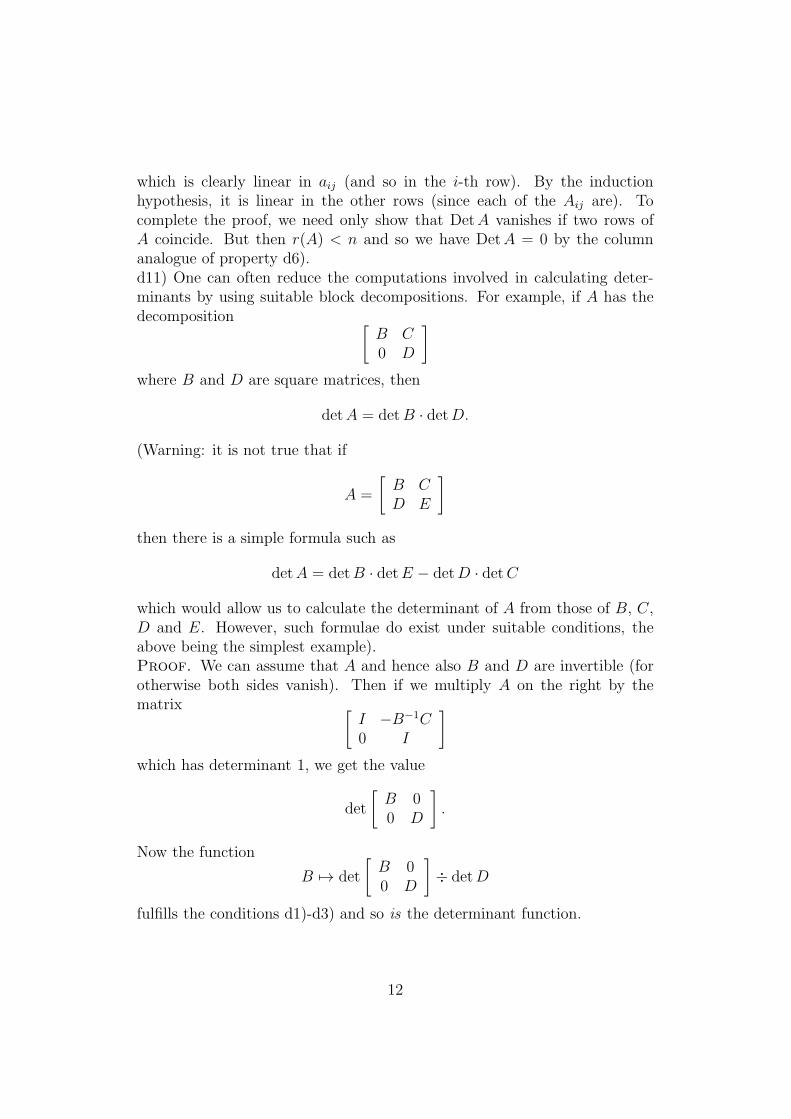
which is clearly linear in aij (and so in the i-th row). By the inductionhypothesis, it is linear in the other rows (since each of the Aij are). Tocomplete the proof, we need only show that DetA vanishes if two rows ofA coincide. But then r(A) < n and so we have DetA = 0 by the columnanalogue of property d6).d11) One can often reduce the computations involved in calculating deter-minants by using suitable block decompositions. For example, if A has thedecomposition [
B C0 D
]
where B and D are square matrices, then
detA = detB · detD.
(Warning: it is not true that if
A =
[B CD E
]
then there is a simple formula such as
detA = detB · detE − detD · detC
which would allow us to calculate the determinant of A from those of B, C,D and E. However, such formulae do exist under suitable conditions, theabove being the simplest example).Proof. We can assume that A and hence also B and D are invertible (forotherwise both sides vanish). Then if we multiply A on the right by thematrix [
I −B−1C0 I
]
which has determinant 1, we get the value
det
[B 00 D
].
Now the function
B 7→ det
[B 00 D
]÷ detD
fulfills the conditions d1)-d3) and so is the determinant function.
12

Determinants of linear operators Since square matrices are the coordi-nate versions of linear operators on a vector space V it is tempting to extendthe definition of determinants to such operators. The obvious way to do thisis to choose some basis (x1, . . . , xn) and to define the determinant det f of fto be the determinant of the matrix of f with respect to this basis. We mustthen verify that this value is independent of the choice of basis. But if A′ isthe matrix of f with respect to another basis, we know that
A′ = S−1AS
for some invertible matrix S. Then we have
detA′ = det(S−1AS)
= detS−1 · detS · detA= det(S−1S) detA
= detA.
Of course, it is essential to employ the matrix of f with respect to a singlebasis for calculating the determinant.
Some of the properties of the determinant can now be interpreted asfollows:a) det f 6= 0 if and only if f is an isomorphism;b) det(fg) = det f · det g (f, g ∈ L(V ));c) det Id = 1.
Example: Calculate
det
6 0 2 04 0 0 20 1 2 02 0 2 2
We have
det
6 0 2 04 0 0 20 1 2 02 0 2 2
= − det
6 2 04 0 22 2 0
= −8 det
3 1 02 0 11 1 0
= −8(−3 + 1) = 16.
13

Example: Calculate
det
x 1 1 11 x 1 11 1 x 11 1 1 x
.
Solution: We have
det
x 1 1 11 x 1 11 1 x 11 1 1 x
= det
0 1− x 1− x2 1− x2
0 −(1 − x) 0 1− x0 0 −(1− x) 1− x1 1 1 x
= det
1− x 1− x 1− x2
−(1 − x) 0 1− x0 −(1− x) 1− x
= (x− 1)3 det
1 1 1 + x−1 0 10 −1 1
= (x− 1)3(1 + x+ 2) = (x− 1)3(3 + x).
Example: Calculate the determinant dn of the n× n matrix
2 −1 0 . . . 0−1 2 0 . . . 0...
...0 0 . . . −1 2
We can express the determinant in terms of the following (n− 1)× (n − 1)determinants by expanding along the first row:
dn = det
2 −1 0 . . . 0−1 2 0 . . . 0...
...0 0 0 . . . 2
+ det
−1 0 0 . . . 0−1 2 −1 . . . 0......0 0 0 . . . 2
= 2dn−1 − dn−2
. It then follows easily by induction that dn = n+ 1.
14

Example: Calculate
det
0 0 . . . 0 10 0 . . . 1 0...
...1 0 . . . 0 0
.
We have
det
0 0 . . . 0 10 0 . . . 1 0...
...1 0 . . . 0 0
= (−1)n det
0 . . . 0 10 . . . 1 0...
...1 . . . 0 0
where the left hand matrix is n×n and the right hand one is (n−1)×(n−1).From this it follows that the value of the given determinant is
(−1)n−1(−1)n−2 . . . (−1)2−1 = (−1)n(n−1)
2 .
Example: Calculate
det
x a a . . . aa x a . . . a...
...a a a . . . x
.
Solution: The required determinant is
det
x a a . . . aa− x x− a 0 . . . a
......
a− x 0 0 . . . x− a
= x(x− a)n−1 − (a− x)a(x− a)n−2 + · · ·+
= x(x− a)n−1 + a(x− a)n−1 + · · ·+= (x+ (n− 1)a)(x− a)n−1.
Example: Calculate the determinant of the Vandermonde matrix
1 x1 x22 . . . xn−11
1 x2 x22 . . . axn−12
......
1 xn x2n . . . xn−1n
.
15
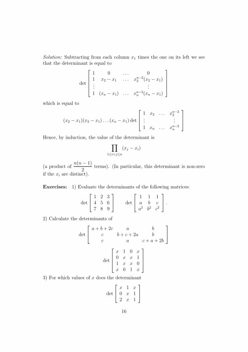
Solution: Subtracting from each column x1 times the one on its left we seethat the determinant is equal to
det
1 0 . . . 01 x2 − x1 . . . xn−2
2 (x2 − x1)...
...1 (xn − x1) . . . xn−2
n (xn − x1)
which is equal to
(x2 − x1)(x3 − x1) . . . (xn − x1) det
1 x2 . . . xn−22
......
1 xn . . . xn−2n
Hence, by induction, the value of the determinant is∏
1≤i<j≤n
(xj − xi)
(a product ofn(n− 1)
2terms). (In particular, this determinant is non-zero
if the xi are distinct).
Exercises: 1) Evaluate the determinants of the following matrices:
det
1 2 34 5 67 8 9
det
1 1 1a b ca2 b2 c2
.
2) Calculate the determinants of
det
a+ b+ 2c a b
c b+ c+ 2a bc a c+ a + 2b
det
x 1 0 x0 x x 11 x x 0x 0 1 x
3) For which values of x does the determinant
det
x 1 x0 x 12 x 1
16

vanish?4) Evaluate the following determinants:
det
1 2 3 . . . n2 3 4 . . . 1...
...n 1 2 . . . n− 1
det
0 1 1 . . . 1−1 0 1 . . . 1...
...−1 −1 −1 . . . 0
det
1 −a 0 . . . 0−b 1 −a . . . 00 −b 1 . . . 0...
...0 0 . . . −b 1
det
λ1 1 0 . . . 0−1 λ2 1 . . . 0...
...0 0 . . . −1 λn
det
λ1 a a . . . ab λ2 a . . . a...
...b b b . . . λn
det
λ a 0 . . . 0a λ a . . . 0...
...0 0 . . . a λ
.
5) Show that if P is a projection, then the dimension k of the range of P isdetermined by the equation
2k = det(I + P ).
Use this to show that if t 7→ P (t) is a continuous mapping from R into thefamily of all projections on Rn, then the dimension of the range of P (t) isconstant.
17
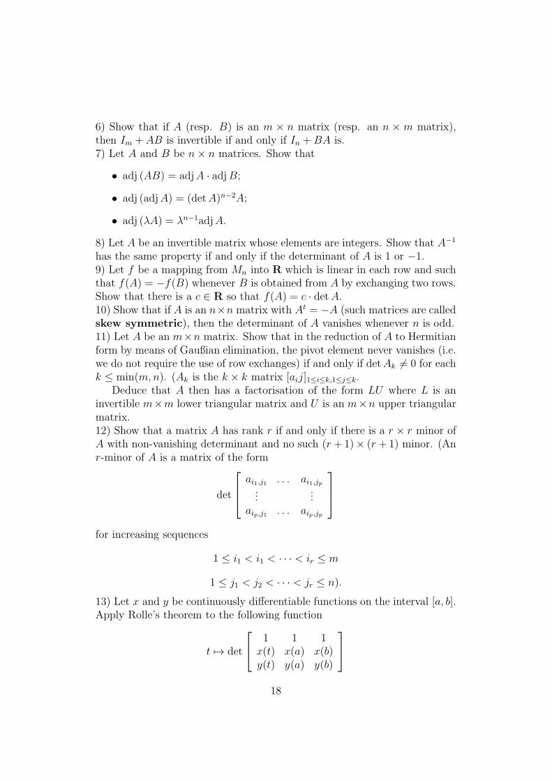
6) Show that if A (resp. B) is an m × n matrix (resp. an n × m matrix),then Im + AB is invertible if and only if In +BA is.7) Let A and B be n× n matrices. Show that
• adj (AB) = adjA · adjB;
• adj (adjA) = (detA)n−2A;
• adj (λA) = λn−1adjA.
8) Let A be an invertible matrix whose elements are integers. Show that A−1
has the same property if and only if the determinant of A is 1 or −1.9) Let f be a mapping from Mn into R which is linear in each row and suchthat f(A) = −f(B) whenever B is obtained from A by exchanging two rows.Show that there is a c ∈ R so that f(A) = c · detA.10) Show that if A is an n×n matrix with At = −A (such matrices are calledskew symmetric), then the determinant of A vanishes whenever n is odd.11) Let A be an m×n matrix. Show that in the reduction of A to Hermitianform by means of Gaußian elimination, the pivot element never vanishes (i.e.we do not require the use of row exchanges) if and only if detAk 6= 0 for eachk ≤ min(m,n). (Ak is the k × k matrix [aij]1≤i≤k,1≤j≤k.
Deduce that A then has a factorisation of the form LU where L is aninvertible m×m lower triangular matrix and U is an m×n upper triangularmatrix.12) Show that a matrix A has rank r if and only if there is a r × r minor ofA with non-vanishing determinant and no such (r+ 1)× (r+ 1) minor. (Anr-minor of A is a matrix of the form
det
ai1,j1 . . . ai1,jp...
...aip,j1 . . . aip,jp
for increasing sequences
1 ≤ i1 < i1 < · · · < ir ≤ m
1 ≤ j1 < j2 < · · · < jr ≤ n).
13) Let x and y be continuously differentiable functions on the interval [a, b].Apply Rolle’s theorem to the following function
t 7→ det
1 1 1x(t) x(a) x(b)y(t) y(a) y(b)
18

Which well-known result of analysis follows?14) Let
x1 = rc1c2 . . . cn−2cn−1
x2 = rc1 . . . cn−2sn−1
...
xj = rc1 . . . cn−jsn−j+1
...
xn = rs1.
where ci = cos θi, si = sin θi (these are the equations of the transformation topolar coordinates in n dimensions). Calculate the determinant of the Jacobimatrix
∂(x1, x2, . . . , xn)
∂(r, θ1, . . . , θn−1).
15) Consider the Vandermonde matrix
Vn =
1 . . . 1t1 . . . tn...
...tn−11 . . . tn−1
n
.
Show that VnVtn is the matrix
s0 s1 . . . sn−1
s1 s2 . . . sn...
...sn−1 sn . . . s2n−2
where sk =∑n
i=1 tki . Use this to calculate the determinant of this matrix.
16) Suppose that the square matrix A has a block representation
[B CD E
]
where B is square and non-singular. Show that
detA = detB det(E −DB−1C).
Deduce that ifD is also square and commutes with B, then detA = det(BE−DC).17) Suppose that A0, . . . , Ar are complex n × n matrices and consider thematrix function
p(t) = A0 + A1t+ · · ·+ Artr.
Show that if det p(t) is constant, then so is p(t) (i.e. A0 is the only non-vanishing term).
19

1.4 Applications of the determinant
We conclude this chapter by listing briefly some applications of the determi-nant:
I. Solving systems of equations—Cramer’s rule: returning to one ofour original motivations for introducing determinants, we show that if thedeterminant of the matrix A of the system AX = Y is non-zero, then theunique solution is given by the formulae
xi =detAi
detA
where Ai is the matrix obtained by replacing the i-th column of A with thecolumn vector Y . To see this note that we can write the system in the form
x1
a11...an1
+ · · ·+
x1a1i − y1
...x1ani − yn
+ · · ·+ xn
x1a1n − y1
...x1ann − yn
= 0
and this just means that the columns of the matrixa11 . . . a1,i−1 (x1a1i − y1) . . . a1n...
...an1 . . . an,i−1 (xiani − yn) . . . ann
are linearly independent. Hence its determinant vanishes and, using thelinearity in the i-th column, this means that detAi − xi detA = 0.
II. The recognition of bases: If (x1, . . . , xn) is a basis for a vector spaceV (e.g. the canonical basis for Rn), then a set (x′1, . . . , x
′n) is a basis if and
only if the determinant of the transfer matrix T = [tij ] whose columns arethe coordinates of the x′j with respect to the (xi) is non-zero.
III. Areas, volumes etc.: If ξ, η are points in R, then
det
[η 1ξ 1
]= η − ξ
is the directed length of the interval from ξ to η.If A = (ξ1, ξ2), B = (η1, η2), C = (ζ1, ζ2) are points in the plane, then
1
2det
ξ1 ξ2 1η1 η2 1ζ1 ζ2 1
20

is the area of the triangle ABC. The area is positive if the direction A →B → C is clockwise, otherwise it is negative. (By taking the signed area weassure that it is additive i.e. that
△ABC = △OAB +△OBC +△OCA
regardless of the position of O with respect to the triangle (see figure ??).If A = (ξ1, ξ2, ξ3), B = (η1, η2, η3), C = (ζ1, ζ2, ζ3), D = (υ1, υ2, υ3) are
points in space, then
1
3!det
ξ1 ξ2 ξ3 1η1 η2 η3 1ζ1 ζ2 ζ3 1υ1 υ2 υ3 1
is the volume of the tetrahedron ABCD.Of course, analogous formulae hold in higher dimensions.
IV. The action of linear mappings on volumes: If f is a linear map-ping from R3 into R3 with matrix
A =
a11 a12 a13a21 a22 a23a31 a32 a33
then f multiplies volumes by a factor of det f . For suppose that f maps thetetrahedron BCDE into the tetrahedron B1C1D1E1. The area of BCDE is
1
3!det
ξ1 ξ2 ξ3 1η1 η2 η3 1ζ1 ζ2 ζ3 1υ1 υ2 υ3 1
where B is the point (ξ1, ξ2, ξ3) etc. and that of the image is
1
3!det
ξ11 ξ12 ξ13 1η11 η12 η13 1ζ11 ζ12 ζ13 1υ1 υ2 υ3 1
.
Now we have
1
3!det
ξ11 ξ12 ξ13 1η11 η12 η13 1ζ11 ζ12 ζ13 1υ1 υ2 υ3 1
=
1
3!det
ξ11 ξ12 ξ13 1η11 η12 η13 1ζ11 ζ12 ζ13 1υ11 υ12 υ13 1
At 0
0 1
21
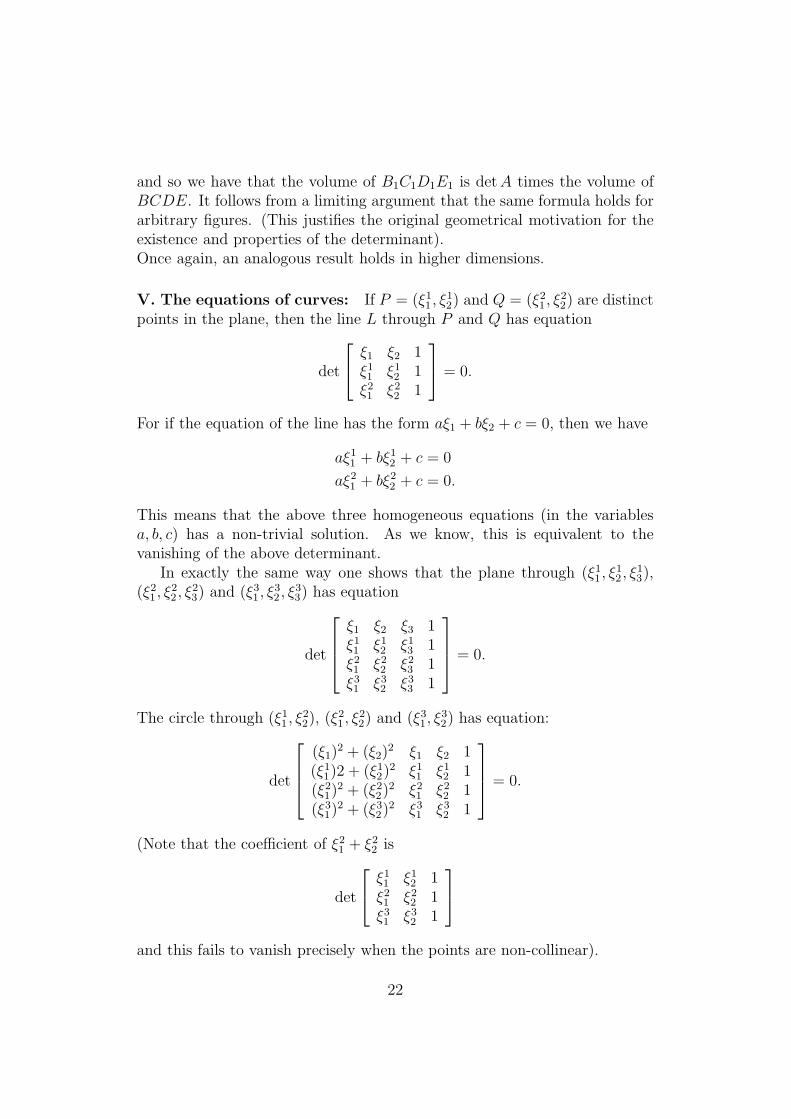
and so we have that the volume of B1C1D1E1 is detA times the volume ofBCDE. It follows from a limiting argument that the same formula holds forarbitrary figures. (This justifies the original geometrical motivation for theexistence and properties of the determinant).Once again, an analogous result holds in higher dimensions.
V. The equations of curves: If P = (ξ11 , ξ12) and Q = (ξ21 , ξ
22) are distinct
points in the plane, then the line L through P and Q has equation
det
ξ1 ξ2 1ξ11 ξ12 1ξ21 ξ22 1
= 0.
For if the equation of the line has the form aξ1 + bξ2 + c = 0, then we have
aξ11 + bξ12 + c = 0
aξ21 + bξ22 + c = 0.
This means that the above three homogeneous equations (in the variablesa, b, c) has a non-trivial solution. As we know, this is equivalent to thevanishing of the above determinant.
In exactly the same way one shows that the plane through (ξ11 , ξ12 , ξ
13),
(ξ21 , ξ22 , ξ
23) and (ξ31 , ξ
32 , ξ
33) has equation
det
ξ1 ξ2 ξ3 1ξ11 ξ12 ξ13 1ξ21 ξ22 ξ23 1ξ31 ξ32 ξ33 1
= 0.
The circle through (ξ11 , ξ22), (ξ
21 , ξ
22) and (ξ31, ξ
32) has equation:
det
(ξ1)2 + (ξ2)
2 ξ1 ξ2 1(ξ11)2 + (ξ12)
2 ξ11 ξ12 1(ξ21)
2 + (ξ22)2 ξ21 ξ22 1
(ξ31)2 + (ξ32)
2 ξ31 ξ32 1
= 0.
(Note that the coefficient of ξ21 + ξ22 is
det
ξ11 ξ12 1ξ21 ξ22 1ξ31 ξ32 1
and this fails to vanish precisely when the points are non-collinear).
22
VI. Orientation: A linear isomorphism f on a vector space V is saidto preserve orientation if its determinant is positive—otherwise it reversesorientation. This concept is particularly important for isometries and thosewhich preserve orientation are called proper. Thus the only proper isome-tries of the plane are translations and rotations.
Two bases (x1, . . . , xn) and (x′1, . . . , x′n) have the same orientation if
the linear mapping which maps xi onto x′i for each i preserves orientation.
This just means that the transfer matrix from (xi) to (x′j) has positive de-
terminant. For instance, in R3, (e1, e2, e3) and (e3, e1, e2) have the sameorientation, whereas that of (e2, e1, e3) is different.
Example Is
cosα cos β sinα cos β − sin βcosα sin β sinα sin β cos β− sinα cosα 0
the matrix of a rotation?Solution: Firstly the columns are orthonormal and so the matrix induces anisometry. but the determinant is
− sin2 α cos2 β − cos2 α sin2 β − sin2 α sin2 β − cos2 α cos2 β = −1.
Hence it is not a rotation.
Example: Solve the system
(m+ 1)x + y + z = 2−mx + (m+ 1)y + z = −2x + y + (m+ 1)z = m.
The determinant of the matrix A of the equation is m2(m + 3) which isnon-zero, unless m = 0 or m = −3. Otherwise the solution is, by Cramer’srule,
x =1
m2(m+ 3)det
2−m 1 1−2 m+ 1 1m 1 m+ 1
i.e.2−m
m. The values of y and z can be calculated similarly.
23

Exercises: 1) Show that the centre of the circle through the points (ξ11 , ξ22),
(ξ21 , ξ22) and (ξ31 , ξ
32) has coordinates
(12det
(ξ11)2 + (ξ12)
2 ξ12 1(ξ21)
2 + (ξ22)2 ξ22 1
(ξ31)2 + (ξ32)
2 ξ32 1
, 1
2det
(ξ11)2 + (ξ12)
2 ξ11 1(ξ21)
2 + (ξ22)2 ξ21 1
(ξ31)2 + (ξ32)
2 ξ31 1
)
det
ξ11 ξ22 1ξ21 ξ22 1ξ31 ξ32 1
.
2) Show that in Rn the equation of the hyperplane through the affinelyindependent points x1, . . . , xn is
det
ξ1 ξ2 . . . ξn 1ξ11 ξ12 . . . ξ1n 1...
...ξn1 ξn2 . . . ξnn 1
= 0.
3) Let A be an invertible n× n matrix. Use that fact that if AX = Y , thenAX = Y where
X =
x1 0 . . . 0x2 1 . . . 0...
...xn 0 . . . 1
Y =
y1 a12 . . . a1ny2 a22 . . . a2n...
...yn an2 . . . ann
to give an alternative proof of Cramer’s rule.4) Let
p(t) = a0 + · · ·+ amtm
q(t) = b0 + · · ·+ bntn
be polynomials whose leading coefficients are non-zero. Show that they havea common root if and only if the determinant of the (m+n)×(m+n) matrix
A =
am am−1 . . . a1 a0 0 . . . 00 am . . . a2 a1 a0 . . . 0...
...0 0 . . . 0 am am−1 . . . a0bn bn−1 . . . b1 b0 0 . . . 0...
...0 0 . . . bn . . . b0
24

is non-zero. (This is known as Sylvester’s criterium for the existence of acommon root). In order to prove it calculate the determinants of the matricesB and BA where B is the (m+ n)× (m+ n) matrix
tn+m−1 0 0 . . . 0tn+m−2 1 0 . . . 0tn+m−3 0 1 . . . 0
......
t 0 0 . . . 01 0 0 . . . 0...
...1 . . . 1
.
25

2 COMPLEX NUMBERS AND COMPLEX
VECTOR SPACES
2.1 The construction of C
When we discuss the eigenvalue problem in the next chapter, it will be con-venient to consider complex vector spaces i.e. those for which the complexnumbers play the role taken by the reals in the third chapter. We thereforebring a short introduction to the theme of complex numbers.
Complex numbers were stumbled on by the renaissance mathematicianCardano in the famous formulae
λ1 =3√α + 3
√β λ2 = ω 3
√α + ω2 3
√β λ3 = ω2 3
√α+ ω 3
√β
where α =−q +
√q2 + 4p3
2, β =
−q −√q2 + 4p3
2, ω =
−1 +√3i
2for the
roots λ1,λ2 and λ3 of the cubic equation
x3 + 3px = q = 0
(which he is claimed to have stolen from a colleague). In the above formulaei denotes the square root of −1 i.e. a number with the property that i2 = −1.This quantity appears already in the solution of the quadratic equation byradicals but only in the case where the quadratic has no real roots. Inthe cubic equation, its occurrence is unavoidable, even in the case wherethe discriminant q2 + 4p3 is positive, in which case the cubic has three realroots. Since the square of a real number is positive, no such number with thedefining property of i exists and mathematicians simply calculated formallywith expressions of the form x+ iy as if the familiar rules of arithmetic stillhold for such expressions. Just how uncomfortable they were in doing this isillustrated by the following quotation from Leibniz:
• “The imaginary numbers are a free and marvellous refuge of the divineintellect, almost an amphibian between existence and non-existence.”
The nature of the complex numbers was clarified by Gauß in the nine-teenth century with the following geometrical interpretation¿ the real num-bers are identified with the points on the x-axis of a coordinate plane. Oneassociates the number i with the point (0, 1) on the plane and, accordingly,the number x + iy with the point (x, y). The arithmetical operations ofaddition and multiplication are defined geometrically as in the following fig-ure (where the triangles OAB and OCD are similar). A little analyticalgeometry shows that these operations can be expressed as follows:
26

addition: (x, y) + (x1, y1) = (x+ x1, y + y1)’multiplication: (x, y) · (x1, y1) = (xx1 − yy1, xy1 + x1y).
Note that these correspond precisely to the expressions obtained by formallyadding and multiplying x+ iy and x1 + iy1.
This leads to the following definition: a complex number is an orderedpair (x, y) of real numbers. On the set of such numbers we define additionand multiplication by the above formulae. We use the following conventions:
• 1) i denotes the complex number (0, 1) and we identity the real numberx with the complex number (x, 0). Then i2 = −1 since
(0, 1) · (0, 1) = (−1, 0).
Every complex number (x, y) has a unique representation x = iy wherex, y ∈ R. (It is customary to use letters such as z, w, . . . for complexnumbers). If z = x+ iy (x, y ∈ R), then x is called the real part of z(written ℜz) and y is called the imaginary part (written ℑz).
• 2) If z = x+ iy, we denote the complex number x− iy (i.e. the mirrorimage of z in the x-axis) by z—the complex-conjugate of z. Thenthe following simple relations holds:
z + z1 = zz1;
zz1 = z · z1;
ℜz = 1
2(z + z);
ℑz = 1
2i(z − z);
z · z = |z|2 where |z| =√x2 + y2.
|z| is called the modulus or absolute value of z. It is multiplicativein the sense that |zz1| = |z||z1|.
• 3) every non-zero complex number z has a unique representation of theform
ρ(cos θ + i sin θ)
where ρ > 0 and θ ∈ [0, 2π[. Here ρ = |z| and θ is the unique real
number in [0, 2π[ so that cos θ =x
ρ, sin θ =
y
ρ.
We denote the set of complex numbers by C. Of course, as a set, it isidentical with R2 and we use the notation C partly for historical reasons andpartly to emphasis the fact that we are considering it not just as a vectorspace but also with its multiplicative structure.
27

Proposition 5 For complex numbers z, z1, z2, z3 we have the relationships
• z1 + z2 = z2 + z1;
• z1 + (z2 + z3) = (z1 + z2) + z3;;
• z1 = 0 = 0 + z1 = z1’
• z1 + (−z1) = 0 where − z1 = (−1)z1;
• z1(z2 + z3) = z1z2 + z1z3;
• z1z2 = z2z1;
• z1(z2z3) = (z1z2)z3;
• z1 · 1 = 1 · z1 = z1;
• if z 6= 0, there is an element z−1 so that z · z−1 = 1 (take z−1 =z
|z|2 ).
This result will be of some importance for us since in our treatment of linearequations, determinants, vector spaces and so on, the only properties of thereal numbers that we have used are those which correspond to the abovelist. Hence the bulk of our definitions, results and proofs can be carried overalmost verbatim to the complex case and, with this justification, we shall usethe complex versions of results which we have proved only for the real casewithout further comment.
It is customary to call a set with multiplication and addition operationswith such properties a field. A further example of a field is the set Q ofrational numbers.
de Moivre’s formula: The formula for multiplication of complex numbershas a particularly transparent form when the complex numbers are repre-sented in polar form: we have
ρ1(cos θ1 + i sin θ1)ρ2(cos θ2 + i sin θ2) = ρ1ρ2(cos(θ1 + θ2) + i sin(θ1 + θ2)).
This is derived by multiplying out the left hand side and using the additionformulae for the trigonometric functions.
This equation can be interpreted geometrically as follows: multiplicationby the complex number z = ρ(cos θ + i sin θ) has the effect of rotating asecond complex number through an angle of θ and multiplying its absolutevalue by ρ (of course this is one of the similarities considered in the second
28

chapter—in fact, a rotary dilation). As a Corollary of the above formula wehave the famous result
(cos θ + i sin θ)n = cosnθ + i sinnθ
of de Moivre. It is obtained by a simple induction argument on n ∈ N.Taking complex conjugates gives the result for −n and so it holds for eachn ∈ Z.
From it we can deduce the following fact: if z = ρ(cos θ + i sin θ) is anon-zero complex number, then there are n solutions of the equation ζn = z(n ∈ N) given by the complex numbers
ρ1n (cos
2πr + θ
n+ sin
2πr + θ
n)
(r = 0, 1, . . . , n−1). In particular, there are n roots of unity (i.e. solutions ofthe equations ζn = 1), namely the complex numbers 1, ω, ω2, . . . , ωn−1 whereω = cos 2π
n+ i sin 2π
nis the primitive n-th root of unity.
Example: If z is a complex number, not equal to one, show that
1 + z + z2 + · · ·+ zn =1− zn+1
1− z.
Use this to calculate the sums
1 + cos θ + · · ·+ cosnθ
andsin θ + · · ·+ sinnθ.
Solution: The first part is proved exactly as in the case of the partial sumsof a real geometric series. If we set z = cos θ + i sin θ and take the real part,we get
1 + cos θ + · · ·+ cosnθ = ℜ1− cos(n+ 1)θ − i sin(n + 1)θ
1− cos θ − i sin θ
which simplifies to the required formula (we leave the details to the reader).The sine part is calculated with the aid of the imaginary part. Example:Describe the geometric form of the set
C = {z ∈ C : zz + az + az + b = 0}
where a is a complex number and b a real number.
29

Solution Substituting z = x+ iy we get
C = {(x, y) : x2 + y2 + 2a1x+ 2a2y + b = 0}
(where a = a1 + ia2) which is a circle, a point or the empty set dependingon the values of a1, a2 and b.
Exercises on complex numbers: 1) Calculate ℜz, ℑz, |z|, z−1 and arg zwhere
z = 1− i z = 3 +√2i
1 + i
1− i.
Show that if z1, z2 ∈ C are such that z1z2 and z1 + z2 are real, then eitherz1 = z2 or z1 and z2 are themselves real.2) If x, x1, y, y1 ∈ R and X = diag(x, x), Y = diag(y, y) etc. while J =[
0 1−1 0
], calculate (X + JY )(X − JY ), (X + JY )(X1 + JY1), (X + JY )−1
(when it exists) and det(X +JY ). (Compare the results with the arithmeticoperations in C. This exercise can be used as the basis for an alternativeconstruction of the complex numbers).3) Use de Moivre’s theorem to derive a formula for cos4 θ in terms of cos 2θand cos 4θ.4) Show that if n is even, then
cosnθ = cosn θ −(n
2
)cosn−2 θ sin2 θ + · · ·+ (−1)
n2 sinn θ;
sinnθ =
(n
1
)cosn−1 θ sin θ + · · ·+ (−1)
n2−1n cos θ sinn−1 θ.
What are the corresponding results for n odd?5) Suppose that |r| < 1. Calculate
1 + r cos θ + r2 cos 2θ + . . .
andr sin θ + r2 sin 2θ + . . .
6) Show that the points z1, z2 and z3 in the complex plane are the verticesof an equilateral triangle if and only if
z1 + ωz2 + ω2z3 = 0
orz1 + ω2z2 + ωz3 = 0
30
where ω = e2πi3 .
If z1, z2, z3, z4 are four complex numbers, what is the geometrical signifi-cance of the condition
z1 + iz2 + (i2)z3 + (i3)z4 = 0?
(Note that i is the primitive fourth root of unity).7) Show that if z1, z2, z3, z4 are complex numbers, then
(z1 − z4)(z2 − z3) + (z2 − z4)(z3 − z1) + (z3 − z4)(z1 − z2) = 0.
Deduce that if A,B,C,D are four points in the plane, then
|AD||BC| ≤ |BD||CA|+ |CD||AB|.
8) We defined the complex numbers formally as pairs of real numbers. Inthis exercise, we investigate what happens if we continue this process i.e. weconsider pairs (z, w) of complex numbers. On the set Q of such pairs wedefine the natural addition and multiplication as follows:
(z0, w0)(z1, w1) = (z0z1 − w0w1, z0w1 + z1w0).
Show that Q satisfies all of the axioms of a field with the exception of thecommutativity of multiplication (such structures are called skew fields).Show that if we put i = (i, 0), j = (0, i), k = (0, 1), then ij = −ji = k,jk = −kj = i etc. and i2 = j2 = k2 = −1. Also every element of Q has aunique representation of the form
ξ0 + (ξ1i+ ξ2j + ξ3k)
with ξ0, ξ1, ξ2, ξ3 ∈ R. (The elements of Q are called quaternions).
31

2.2 Polynomials
The field of complex numbers has one significant advantage over the realfield. All polynomials have roots. This result will be very useful in the nextchapter—it is known as the fundamental theorem of algebra and canbe stated in the following form:
Proposition 6 Let
p(λ) = a0 + · · ·+ an−1λn−1 + λn
be a complex polynomial with n ≥ 1. Then there are complex numbersλ1, . . . , λn so that
p(λ) = (λ− λ1) . . . (λ− λn).
There is no simple algebraic proof of this result which we shall take forgranted.
The fundamental theorem has the following Corollary on the factorisationof real polynomials.
Corollar 1 Letp(t) = a0 + · · ·+ an−1t
n−1 + tn
be a polynomial with real coefficients. Then there are real numbers
t1, . . . , tr, α1, . . . , αs, β1, . . . , βs
where r + 2s = n so that
p(t) = (t− t1) . . . (t− tr)(t2 − 2α1t+ α2
1 + β21) . . . (t
2 − 2αst + α2s + β2
s ).
Proof. We denote by λ1, . . . , λn the complex roots of the polynomial
p(λ) = a0 + a1λ+ · · ·+ λn.
Since p(λ) = p(λ) (the coefficients being real), we see that a complex numberλ is a root if and only if its complex conjugate is also one. Hence we can listthe roots of p as follows: firstly the real ones
t1, . . . , tr
and then the complex ones in conjugate pairs:
α1 + iβ1, α1 − iβ1, . . . , αs + iβs, αs − iβs.
32
Then we see that p has the required form by multiplying out the correspond-ing linear and quadratic terms.
The next result concerns the representation of rational functions. These
are functions of the formp
qwhere p and q are polynomials. By long division
every such function can be expressed as the sum of a polynomial and a
rational functionildep
qwhere the degree d(p) of p (i.e. the index of its highest
power) is strictly less than that of q. Hence from now on we shall tacitlyassume that this condition is satisfied. Further it is no loss of generality tosuppose that the leading coefficient of q is “1”.
We consider first the case where q has simple zeros i.e.
q(λ) = (λ− λ1) . . . (λ− λn)
where the λi are distinct. Then we claim that there are uniquely determinedcomplex numbers a1, . . . , an so that
p(λ)
q(λ)=
a1λ− λ1
+ . . .an
λ− λN
for λ ∈ C \ {λ1, . . . , λn}.Proof. This is equivalent to the equation
p(λ) =
n∑
i=1
aiqi(λ)
where qi(λ) =q(λ)λ−λi
. If this holds for all λ as above then it holds for all λ inC since both sides are polynomials. Substituting successively λ1,λ2, . . . , λnin the equation we see that
a1 =p(λ1)
(λ1 − λ2) . . . (λ1 − λn)...
an =p(λn)
(λ2 − λn) . . . (λn − (λn−1
The general result (i.e. where q has multiple zeros) is more complicated tostate. We suppose that
q(λ) = (λ− λ1)n−1 . . . (λ− λr)
nr
where the λi are distinct and claim that the rational function can be writtenas a linear combination of functions of the form 1
(λ−λi)jfor 1 ≤ i ≤ r and
1 ≤ j ≤ ni.
33
Proof. Writep(λ)
q(λ)=
p(λ)
(λ− λ1)n1q1(λ)
where q1(λ) = (λ− λ2)n2 . . . (λ− λr)
nr . We claim that there is a polynomialp1 with d(p1) = d(p)− 1 and an a ∈ C so that
p(λ)
(λ− λ1)n1q1(λ)=
a
(λ− λ1)n1+
p1(λ)
(λ− λ1)n1−1q1(λ)
from which the proof follows by induction.For the above equation is equivalent to the following one:
p(λ)− aq1(λ)
q(λ)=
p1(λ)
(λ− λ1)n1−1q(λ).
Hence it suffices to choose a ∈ C so that p(λ) − aq1(λ) contains a factor
λ− λ1 and there is precisely one such a namely a =p(λ1)
q1(λ).
We remark that the degree function satisfies the following properties:
d(p+ q) ≤ max(d(p), d(q))
with equality if d(p) 6= d(q)) and
d(pq) = d(p) + d(q)
provided that p and q are non-zero.The standard high school method for the division of polynomials can be
used to prove the existence part of the following result:
Proposition 7 Let p and q be polynomials with d(p) ≥ 1. Then there areunique polynomials r, s so that
q = ps + r
where r = 0 or d(r) < d(p).
Proof. In the light of the above remark, we can confine ourselves to a proofof the uniqueness: suppose that
q = ps+ r = ps1 + r1
for suitable s, r, s1, r1. Then
p(s− s1) = r − r1.
Now the right hand side is a polynomial of degree strictly less than that of pand hence so is the left hand side. But this can only be the case if s = s1.
34
The above division algorithm can be used to prove an analogue of theEuclidean algorithm for determining the greatest common divisor of twopolynomials p, q. We say that for two such polynomials, q is a divisor ofp (written q | p) if there is a polynomial s so that p = qs. Note that thend(p) ≥ d(q) (where d(p) denotes the degree of p). Hence if p | q and q | p, thend(p) = d(q) and it follows that p is a non-zero constant times q (we are tacitlyassuming that the polynomials p and q are both non-zero). The greatestcommon divisor of p and q is by definition a common divisor which hasas divisor each other divisor of p and q. It is then uniquely determined upto a scalar multiple and we denote it by g.c.d. (p, q). It can be calculated asfollows: we suppose that d(q) ≤ d(p) and use the division algorithm to write
p = qs1 + r1
with r1 = 0 or d(r1) < d(q). In the first case, q is the greatest commondivisor. Otherwise we write
q = s2r1 + r2
thenr1 = s3r2 + r3
and continue until we reach a final equation rk = sk+2rk+1 without remainder.Then rk−1 is the greatest common divisor and by substituting backwardsalong the equations, we can compute a representation of it in the formmp+nqfor suitable polynomials m and n.
Lagrange interpolation A further useful property of polynomials is thefollowing interpolation method: suppose that we have (n+1) distinct pointst0, . . . , tn in R. Then for any complex numbers a0, . . . , an we can find apolynomial p of degree at most n so that p(ti) = ai for each i. To do thisnote that the polynomial
pi(t) =∏
i 6=j
t− tjti − tj
has the property that it takes on the value 1 at ti and 0 at the other tj. Then
p =
n∑
i=0
aipi
is the required polynomial.
35
Exercises: 1) Show that a complex number λ0 is a root of order r of thepolynomial p (i.e. (λ− λ0)
r divides p) if and only if
p(λ0) = p′(λ0) = · · · = p(r−1)(λ0) = 0.
2) Show that, in order to prove the fundamental theorem of algebra, it sufficesto prove that every polynomial p of degree ≥ 1 has at least one zero.3) Prove the statement of 2) (and hence the fundamental theorem of algebra)by verifying the following steps:
• show that if p is a non-constant polynomial, then there is a point λ0 inC so that |p(λ0)| ≤ |p(λ)|(λ ∈ C).
• show that p(λ0) = 0.
(If a0 = p(λ0) is non-zero, consider the Taylor expansion
p(λ) = a0 + ar(λ− λ0)r + · · ·+ an(λ− λ0)
n
of p at λ0 where ar is the first coefficient after a0 which does not vanish.Show that there is a point λ1 so that |p(λ1)| < |a0| which is a contradiction).4) Show that the set of rational functions is a field with the natural algebraicoperations.
36
2.3 Complex vector spaces and matrices
We are now in a position to define complex vector spaces.
Definition: A complex vector space (or vector space over C) is aset V together with an addition and a scalar multiplication i.e. mappings(x, y) 7→ x+ y resp. (λ, x) 7→ λx form V × V into V resp. from C× C intoV so that
• x+ y = y + x (x, y ∈ V )’
• x+ (y + z) = (x+ y) + z (x, y, z ∈ V );
• there is a vector 0 so that x+ 0 = x for each x ∈ V ;
• for each x ∈ V there is a vector y so that x+ y = 0;
• (λµ)x = λ(µx) (λ, µ ∈ C, x ∈ V );
• 1 · x = x (x ∈ V );
• λ(x+ y) = λx+ λy and (λ+ µ)x = λx+ µx (λ, µ ∈ C, x, y ∈ V ).
The following modifications of our examples of real vector spaces provide uswith examples of complex ones:
• Cn—the space of n-tuples (λ1, . . . , λn) of complex numbers;
• PolC (n)—the space of polynomials with complex coefficients of degreeat most n;
• MC
m,n—the space of m× n matrices with complex elements.
We can then define linear dependence resp. independence for elements of acomplex vector space and hence the concept of basis. Every complex vectorspace which is spanned by finitely many elements has a basis and so is iso-morphic to Cn where n is the dimension of the space i.e. the cardinality ofa basis.
If V and W are complex vector spaces, the notion of a linear mappingfrom V into W is defined exactly as in the real case (except, of course, forthe fact that the homogeneity condition f(λx) = λf(x) must now hold for allcomplex λ). Such a mapping f is determined by a matrix [aij ] with respectto bases (x1, . . . , xn) resp. (y1, . . . , yn) where the elements of the matrix arenow complex numbers and are determined by the equations
f(xj) =
m∑
i=1
aijyi.
37
The theory of chapters I and V for matrices can then be carried over in theobvious way to complex matrices.
Sometimes it is convenient to be able to pass between complex and realvectors and this can be achieved as follows: if V is a complex vector space,then we can regard it as a real vector space simply by ignoring the fact thatwe can multiply by complex scalars. We denote this space by V R. Thisnotation may seem rather pedantic—but note that if the dimension of V is nthen that of VR is 2n. This reflects the fact that elements of V can be linearlydependent in V without being so in VR since there are less possibilities forbuilding linear combinations in the latter. For example, the sequence
(1, 0, . . . , 0), (0, 1, . . . , 0), . . . , (0, . . . , 0, 1)
is a basis for Cn whereas the longer sequence
(1, 0, . . . , 0), (i, 0, . . . , 0), (0, 1, . . . , 0), . . . , (0, . . . , 0, i)
is necessary to attain a basis for the real space Cn which is thus 2n dimen-sional.
On the other hand, it V is a real vector space we can define a correspond-ing complex vector space VC as follows: as a set VC is V × V . It has thenatural addition and scalar multiplication is defined by the equation
(λ+ iµ)(x1, x2) = (λx1 − µx2, µx1 + λx2).
The dimensions of V (as a real space) and VC (as a complex space) are thesame. If f : V →W is a linear mapping between complex vector space thenit is a fortiori a linear mapping from VR into WR. However, a real linearmapping between the latter spaces need not be complex-linear. On the otherhand, if f : V → W is a linear mapping between real vector spaces, we canextend it to a complex linear mapping fC between VC and WC by defining
fC(x1, x2) = (f(x1), f(x2)).
Exercises: 1) Solve the system
(1− i)x − 9y = 02x + (1− i)y = 1.
2) Find a Hermitian form for the matrix
i −(1 + i) 11 2 −12i 1 1
.
38

3) Show that if z1, z2, z3 are complex numbers, then
det
z1 z1 1z2 z2 1z3 z3 1
is 4i times the area of the triangle with z1, z2, z3 as vertices.4) Let A and B be real n × n matrices. Show that if A and B are similaras complex matrices (i.e. if there is an invertible complex matrix P so thatP−1AP = B) then they are similar as real matrices (i.e. there is a real matrixP with the same property).5) Let A and B be real n× n matrices. Show that
det(A+ iB = det(A− iB)
and that
det
[A −BB A
]= | det(A + iB)|2.
6) (The following exercise shows that complex 2× 2 matrices can be used togive a natural approach to the two products in R3). Consider the space MC
2
of 2× 2 complex matrices. If A is such a matrix, say
A =
[a11 a22
alpha21 a22
]
then we write A∗ for the matrix[a11 a21a12 a22
].
(The significance of this matrix will be discussed in more detail in ChapterVII). We let E3 denote the family of those A which satisfy the conditionsA = A∗ and trA = 0. The set of such matrices is a real vector space (butnot a complex one). In fact if x = (ξ1, ξ2, ξ3) is an element of R3, then thematrix
Ax =
[ξ3 ξ1 − iξ2
ξ1 + ξ2 −ξ3
]
is in E3. Show that this induces an isomorphism between R3 and E3. Showthat E3 is not closed under (matrix) products but that if A,B ∈ E3, then
A ∗B =1
2(AB + BA)
39

is also in E3 and that
Ax ∗Ay = (x|y)I2 + Ax×y.
7) Complex 2 × 2 matrices also allow a natural approach to the subject ofquaternions (cf. Exercise 8) of section VI.1). Consider the set of matrices ofthe form [
z ww −z
]
where z, w ∈ C. Show that this is closed under addition and multiplicationand that the mapping
(z, w) 7→[z ww −z
]
is a bijection between Q and the set of such matrices which preserves thealgebraic operations. (Note that under this identification, the special quater-nions have the form
ii =
[0 11 0
]j =
[0 −ii 0
]k =
[1 00 −1
]
and that the quaternion ξ0 + ξ1i + ξ2j + ξ3k is represented by the matrixξ0I2 + Ax where Ax is as in exercise 6)).8) Use the results of the last two exercises to give new proofs of the followingidentities involving the vector and scalar products:
x× y = −y × x;
‖x× y‖ = ‖x‖‖y‖ sin θ where θ is the angle between x and y;
(x× y)× z = (x|z)y − (y|z)x;(x× y)× z + (y × z)× x+ (z × x)× y = 0.
40

3 EIGENVALUES
3.1 Introduction
In this chapter we discuss the so-called eigenvalue problem for operatorsor matrices. This means that for a given operator f ∈ L(V ) a scalar λ anda non-zero vector x are sought so that f(x) = λx (i.e. the vector x is notrotated by f). Such problems arise in many situations, some of which weshall become acquainted with in the course of this chapter. In fact, if thereader examines the discussion of conic sections in the plane and three di-mensional space he will recognise that the main point in the proof was thesolution of an eigenvalue problem. The underlying theoretical reason for theimportance of eigenvalues is the following: we know that a matrix is thecoordinate representation of an operator. Even in the most elementary an-alytic geometry one soon appreciates the advantage of choosing a basis forwhich the matrix has a particularly simple form. The simplest possible formis that of a diagonal matrix and the reader will observe that we obtain sucha representation precisely when the basis elements are so-called eigenvectorsof the operator f i.e. they satisfy the condition f(xi) = λixi for suitableeigenvalues λ1, . . . , λn (which then form the diagonal elements of the corre-sponding matrix). Stated in terms of matrices this comprises what we maycall the diagonalisation problem: given an n × n matrix A can we find aninvertible matrix S so that S−1AS is diagonal?
Amongst the advantages that such a diagonalisation brings is the fact thatone can then calculate simply and quickly arbitrary powers and thus poly-nomial functions of a matrix by doing this for the diagonal matrix and thentransforming back. We shall discuss some applications of this below. On theother hand, if A is the matrix of a linear mapping in Rn we can immediatelyread off the geometrical form of the latter from its diagonalisation.
We begin with the formal definition. If f ∈ L(V ), an eigenvalue of fis a scalar λ so that there exists a non-zero x with f(x) = λx. The spaceKer (f − λId) is then non-trivial and is called the eigenspace of λ and eachnon-zero element therein is called an eigenvector. Our main concern inthis chapter will be the following: given an operator f , can we find a basisfor V consisting of eigenvectors? In general the answer is no as very simpleexamples show but we shall obtain a result which, while being much lessdirect, is still useful in theory and applications.
We can restate the eigenvalue problem in terms of matrices: an eigenvalueresp. eigenvector for an n×n matrix A is an eigenvalue resp. eigenvector forthe operator fA i.e. λ is an eigenvalue if and only if there exists a non-zerocolumn vector X so that AX = λX and X is then called an eigenvector.
41
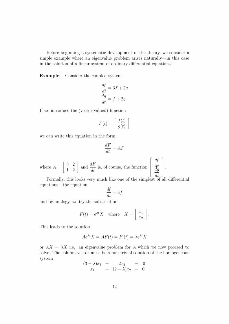
Before beginning a systematic development of the theory, we consider asimple example where an eigenvalue problem arises naturally—in this casein the solution of a linear system of ordinary differential equations:
Example: Consider the coupled system
df
dt= 3f + 2g
dg
dt= f + 2g.
If we introduce the (vector-valued) function
F (t) =
[f(t)g(t)
]
we can write this equation in the form
dF
dt= AF
where A =
[3 21 2
]and
dF
dtis, of course, the function
df
dtdg
dt
.
Formally, this looks very much like one of the simplest of all differentialequations—the equation
df
dt= af
and by analogy, we try the substitution
F (t) = eλtX where X =
[x1x2
].
This leads to the solution
AeλtX = AF (t) = F ′(t) = λeλtX
or AX = λX i.e. an eigenvalue problem for A which we now proceed tosolve. The column vector must be a non-trivial solution of the homogeneoussystem
(3− λ)x1 + 2x2 = 0x1 + (2− λ)x2 = 0.
42

Now we know that such a solution exists if and only if the determinant ofthe corresponding matrix vanishes. This leads to the equation
(3− λ)(2− λ)− 2 = 0
for λ which has solutions λ = 1 or λ = 4.If we solve the corresponding homogeneous systems we get eigenvectors
(−1, 1) and (2, 1) respectively and they form a basis for R2. hence if
S =
[−1 21 1
]
is the matrix whose columns are the eigenvectors of A we see that
S−1AS =
[1 00 4
].
Then our differential equation has the solution
F (t) = c1et
[−11
]+ c2e
4t
[21
]
i.e. f(t) = −c1et + 2ce4t, g(t) = c1et + c2e
4t for arbitrary constants c1, c2.
43

3.2 Characteristic polynomials and diagonalisation
The above indicates the following method for characterising eigenvalues:
Proposition 8 If A is an n× n matrix, then λ is an eigenvalue of A if andonly if λ is a root of the equation
det(A− λI) = 0.
Proof. λ is an eigenvalue if and only if the homogeneous equation AX =λX has a non-trivial solution and the matrix of this equation is A− λI.We remark that det(A− λI) = 0 is a polynomial equation of degree n.
From this simple result we can immediately draw some useful conclusions:I. Every matrix over C has n eigenvalues, the n roots of the above equa-tion (although some of the eigenvalues can occur as repeated roots of theequation).II. Every real matrix has at least one real eigenvalue if n is odd (in particularif n = 3). The example of a rotation in R2 shows that 2× 2 matrices over Rneed not have any eigenvalues.III. If A is a triangular matrix, say
A =
a11 a12 . . . a1n0 a22 . . . a2n...
...0 0 . . . ann
,
then the eigenvalues of A are just the diagonal elements a11, . . . , ann (inparticular, this holds if A is diagonal). For
det(A− λI) = (a11 − λ) . . . (ann − λ)
with roots a11, . . . , ann.Owing to the special role played by the polynomial det(A − λI) in the
eigenvalue problem we give it a special name—the characteristic polyno-mial of A—in symbols χA. For example, if
A =
1 −1 0−1 2 −10 −1 1
then χA(λ) = λ(1− λ)(λ− 3).For an operator f ∈ L(V ), the characteristic polynomial is defined by the
equationχf(λ) = det(f − λId)
44
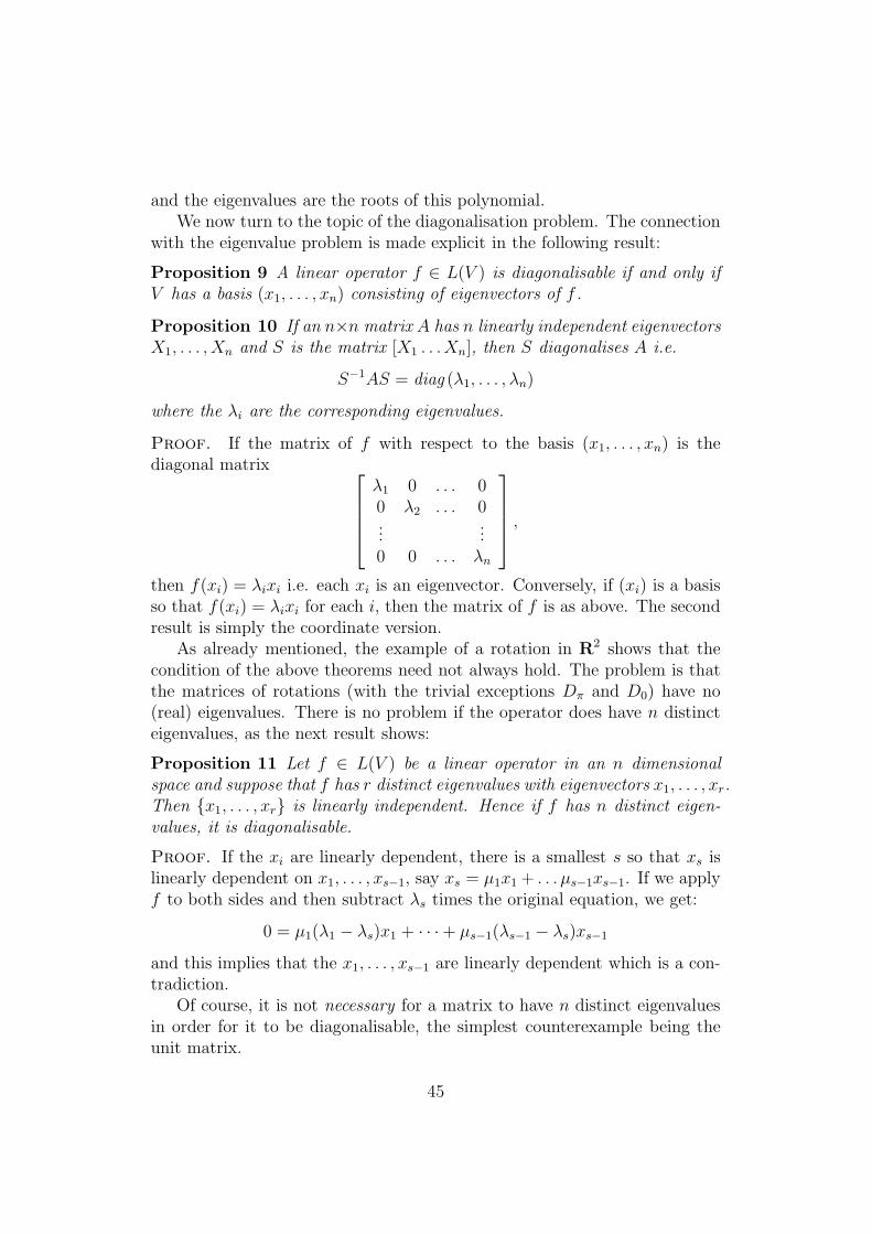
and the eigenvalues are the roots of this polynomial.We now turn to the topic of the diagonalisation problem. The connection
with the eigenvalue problem is made explicit in the following result:
Proposition 9 A linear operator f ∈ L(V ) is diagonalisable if and only ifV has a basis (x1, . . . , xn) consisting of eigenvectors of f .
Proposition 10 If an n×n matrix A has n linearly independent eigenvectorsX1, . . . , Xn and S is the matrix [X1 . . .Xn], then S diagonalises A i.e.
S−1AS = diag (λ1, . . . , λn)
where the λi are the corresponding eigenvalues.
Proof. If the matrix of f with respect to the basis (x1, . . . , xn) is thediagonal matrix
λ1 0 . . . 00 λ2 . . . 0...
...0 0 . . . λn
,
then f(xi) = λixi i.e. each xi is an eigenvector. Conversely, if (xi) is a basisso that f(xi) = λixi for each i, then the matrix of f is as above. The secondresult is simply the coordinate version.
As already mentioned, the example of a rotation in R2 shows that thecondition of the above theorems need not always hold. The problem is thatthe matrices of rotations (with the trivial exceptions Dπ and D0) have no(real) eigenvalues. There is no problem if the operator does have n distincteigenvalues, as the next result shows:
Proposition 11 Let f ∈ L(V ) be a linear operator in an n dimensionalspace and suppose that f has r distinct eigenvalues with eigenvectors x1, . . . , xr.Then {x1, . . . , xr} is linearly independent. Hence if f has n distinct eigen-values, it is diagonalisable.
Proof. If the xi are linearly dependent, there is a smallest s so that xs islinearly dependent on x1, . . . , xs−1, say xs = µ1x1 + . . . µs−1xs−1. If we applyf to both sides and then subtract λs times the original equation, we get:
0 = µ1(λ1 − λs)x1 + · · ·+ µs−1(λs−1 − λs)xs−1
and this implies that the x1, . . . , xs−1 are linearly dependent which is a con-tradiction.
Of course, it is not necessary for a matrix to have n distinct eigenvaluesin order for it to be diagonalisable, the simplest counterexample being theunit matrix.
45

Estimates for eigenvalues For applications it is often useful to have esti-mates for the eigenvalues of a given matrix, rather than their precise values.In this section, we bring two such estimates, together with some applications.
Recall that if a matrix A is dominated by the diagonal in the sense thatfor each i
|aii| −∑
j 6=i
|aij| > 0,
then it is invertible (see Chapter IV). This can be used to give the followingestimate:
Proposition 12 Let A be a complex n×n matrix with eigenvalues λ1, . . . , λn.Put for each i
αi =∑
j 6=i
|aij |.
Then the eigenvalues lie in the region
⋃{z ∈ C : |z − aii| ≤ αi}.
Proof. It is clear that if λ does not lie in one of the above circular regions,then the matrix (λI − A) is dominated by the diagonal in the above senseand so is invertible i.e. λ is not an eigenvalue.
We can use this result to obtain a classical estimate for the zero of poly-nomials. Consider the polynomial p which maps t onto a0 + a1t + · · · +an−1t
n−1+ tn. The roots of p coincide with the eigenvalues of the companionmatrix
C =
0 1 0 . . . 00 0 1 . . . 0...
...−a0 −a1 −a2 . . . −an−1
(see Exercise 4) below).It follows from the above criterium that if λ is a zero of p, then
|λ| ≤ max(|a0|, 1 + |a1|, . . . , 1 + |an−1|).
Our second result shows that the eigenvalues of a small matrix cannot betoo large. More precisely, if A is an n × n matrix and a = maxi,j |aij |, theneach eigenvalue λ satisfies the inequality: |λ| ≤ na. For suppose that
X =
ξ1...ξn
46
is a corresponding eigenvector. Then we have
(AX|X) = λ(X|X)
i.e.λ∑
i
ξiξi =∑
i,j
aijξiξj.
Taking absolute values, we have the inequality
|λ|∑
i
|ξi|2 ≤∑
i,j
|aij ||ξi||ξj|
≤ a∑
i,j
|ξi||ξj|
= a(∑
i
|ξi|)(∑
j
|ξj|)
≤ na(∑
i
|ξi|2)
which implies the result. (In the last inequality, we use the Cauchy-Schwarz
inequality which implies that∑
i |ξi| ≤ n12 (∑
i |ξi|2)12 . See the next chapter
for details).We conclude this section with an application of the diagonalisation method:
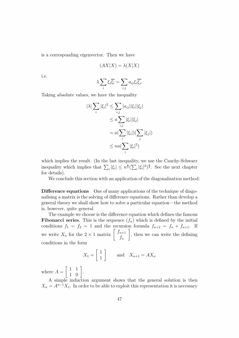
Difference equations One of many applications of the technique of diago-nalising a matrix is the solving of difference equations. Rather than develop ageneral theory we shall show how to solve a particular equation—the methodis, however, quite general.
The example we choose is the difference equation which defines the famousFibonacci series. This is the sequence (fn) which is defined by the initialconditions f1 = f2 = 1 and the recursion formula fn+2 = fn + fn+1. If
we write Xn for the 2 × 1 matrix
[fn+1
fn
], then we can write the defining
conditions in the form
X1 =
[11
]and Xn+1 = AXn
where A =
[1 11 0
].
A simple induction argument shows that the general solution is thenXn = An−1X1. In order to be able to exploit this representation it is necessary
47

to compute the powers of A. To do this directly would involve astronomicalcomputations. The task is simplified by diagonalising A. A simple calculation
shows that A has eigenvalues1 +
√5
2and
1−√5
2, with eigenvectors
[1+
√5
2
1
]and
[1−
√5
2
1
].
Hence
S−1AS =
[1+
√5
20
0 1−√5
2
]
where S =
[1+
√5
21−
√5
2
1 1
].
From this it follows that
A =1√5
[1+
√5
21−
√5
2
1 1
][1+
√5
20
0 1−√5
2
][1 −1−
√5
2
−1 1+√5
2
]
and
An =1√5
[1+
√5
21−
√5
2
1 1
][1+
√5
20
0 1−√5
2
]n [1 −1−
√5
2
−1 1+√5
2
]
This leads to the formula
fn =1√5
[(1 +
√5
2
)n
−(1−
√5
2
)n].
Examples: 1) Calculate χA(λ) where
A =
1 1 . . . 1...
...1 1 . . . 1
.
Solution:
χA(λ) = det
1− λ 1 . . . 1...
...1 1 . . . 1− λ
= (n− λ)λn−1(−1)n−1.
by a result of the previous chapter.
48

2) Calculate the eigenvalues of the n× n matrix
A =
0 1 0 . . . 00 0 1 . . . 0...
...1 0 0 . . . 0
.
Solution:
χA(λ) =
−λ 1 0 . . . 00 λ 1 . . . 0...
...1 0 0 . . . λ
= (−1)n−1(λn − 1).
Hence the eigenvalues are the roots e2πirn of unity (r = 0, . . . , n− 1).
3) Calculate the eigenvalues of the linear mapping[a11 a12a21 a22
]7→[a11 a21a12 a22
]
on M2.Solution: With respect to the basis
x1 =
[1 00 0
]x2 =
[0 10 0
]x3 =
[0 01 0
]x4 =
[0 00 1
]
the mapping has matrix
1 0 0 00 0 1 00 1 0 00 0 0 1
and this has eigenvalues 1, 1, 1,−1.4) Show that fn+1fn−1−f 2
n = (−1)n−1 where fn is the n-th Fibonacci number.Solution: Note the
fn+1fn−1 − f 2n = det
[fn+1 fnfn fn−1
]
= det
[1 11 0
]n−1 [f2 f1f1 f0
]
= (det
[1 11 0
])n−1 det
[2 11 1
]
= (−1)n−1.
.
49

3.3 The Jordan canonical form
As we have seen, not every matrix can be reduced to diagonal form and inthis section we shall investigate what can be achieved in the general case.We begin by recalling that failure to be diagonalisable can result from twocauses. Firstly, the matrix can fail to have a sufficient number of eigenvalues(i.e. zeroes of χA). By the fundamental theorem of algebra, this can onlyhappen in the real case and in this section we shall avoid this difficulty byconfining our attention to complex matrices resp. vector spaces. The seconddifficulty is that the matrix may have n eigenvalues (with repetitions) butmay fail to have enough eigenvectors to span the space. A typical exampleis the shear operator
(ξ1, ξ2) 7→ (ξ1 + ξ2, ξ2)
with matrix
[1 10 1
].
This has the double eigenvalue 1 but the only eigenvectors are multiplesof the unit vector (1, 0). We will investigate in detail the case of repeatedeigenvalues and it will turn out that in a certain sense the shear operatorrepresents the typical situation. The precise result that we shall obtain israther more delicate to state and prove than the diagonalisable case and weshall proceed by way of a series of partial results. We begin with the followingProposition which allows us to reduce to the case where the operator f hasa single eigenvalue.
In order to avoid tedious repetitions we assume from now until the endof this section that f is a fixed operator on a complex vector space V ofdimension and that f has eigenvalues
λ1, . . . , λ1, λ2, . . . , λr, . . . , λr
where λi occurs ni times. This means that f has characteristic polynomial
(λ1 − λ)n1 . . . (λr − λ)nr
where n1 + · · ·+ nr = n).
Proposition 13 There is a direct sum decomposition
V = V1 ⊕ · · · ⊕ Vr
where
• each Vi is f invariant (i.e. f(Vi) ⊂ Vi);
• the dimension of Vi is ni and (f − λiId)ni|Vi
= 0.
In particular, the only eigenvalue of f |Viis λi.
50
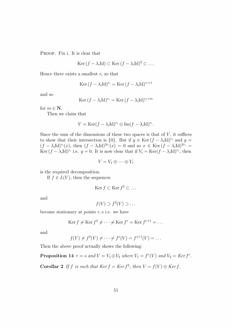
Proof. Fix i. It is clear that
Ker (f − λiId) ⊂ Ker (f − λiId)2 ⊂ . . .
Hence there exists a smallest ri so that
Ker (f − λiId)ri = Ker (f − λiId)
ri+1
and soKer (f − λiId)
ri = Ker (f − λiId)ri+m
for m ∈ N.Then we claim that
V = Ker(f − λiId)ri ⊕ Im(f − λiId)
ri.
Since the sum of the dimensions of these two spaces is that of V , it sufficesto show that their intersection is {0}. But if y ∈ Ker (f − λiId)
ri and y =(f − λiId)
ri(x), then (f − λiId)2ri(x) = 0 and so x ∈ Ker (f − λiId)
2ri =Ker (f − λiId)
ri i.e. y = 0. It is now clear that if Vi = Ker(f − λiId)ri , then
V = V1 ⊕ · · · ⊕ Vr
is the required decomposition.If f ∈ L(V ), then the sequences
Ker f ⊂ Ker f 2 ⊂ . . .
andf(V ) ⊃ f 2(V ) ⊃ . . .
become stationary at points r, s i.e. we have
Ker f 6= Ker f 2 6= · · · 6= Ker f r = Ker f r+1 = . . .
andf(V ) 6= f 2(V ) 6= · · · 6= f s(V ) = f s+1(V ) = . . .
Then the above proof actually shows the following:
Proposition 14 r = s and V = V1⊕V2 where V1 = f r(V ) and V2 = Ker f r.
Corollar 2 If f is such that Ker f = Ker f 2, then V = f(V )⊕Ker f .
51

Using the above result, we can concentrate on the restrictions of f to the sum-mands. These have the special property that they have only one eigenvalue.Typical examples of matrices with this property are the Jordan matriceswhich we introduced in the first chapter. Recall the notation
Jn(λ) =
λ 1 0 . . . 00 λ 1 . . . 0...
...0 0 0 . . . λ
.
In particular, the shear matrix is J1(1).The following facts can be computed easily.
1) Jn(λ) has one eigenvalue, namely λ, and one eigenvector (1, 0, . . . , 0) (orrather multiples of this vector);2) If p is a polynomial, then
p(Jn(λ)) =
p(λ) p′(λ) . . . p(n−1)(λ)(n−1)!
0 p(λ) . . ....
...0 0 . . . p(λ)
.
3) Jn(λ)− λI is the matrix
Jn(0) =
0 1 0 . . . 00 0 1 . . . 0...
...0 0 0 . . . 0
.
Hence (Jn(λ)− λI)n = 0 and (Jn(λ)− λI)r 6= 0 if r < n.The next result shows that all operators with only one eigenvalue can be
represented by blocks of Jordan matrices:
Proposition 15 Let g be a linear operator on the n-dimensional space Wso that (g − λI)n = 0 for some λ ∈ C. Then there is a decomposition
W = W1 ⊕ · · · ⊕Wk
so that eachWi is g-invariant and has a basis with respect to which the matrixof g is the Jordan matrix Jsi(λ) where si = dimWi.
By replacing g by g − λI we can reduce to the following special case whichis the one which we shall prove:
52
Proposition 16 Let g ∈ L(V ) be nilpotent with gr = 0, gr−1 6= 0. Thenthere is a decomposition
V = V1 ⊕ · · · ⊕ Vk
with each Vi g-invariant and a basis for each Vi so that g|Vihas matrix Jsi(0)
where si = dimVi.
Proof. Choose x1 ∈ V so that gr−1(x1) 6= 0. Then the vectors
x1, g(x1), . . . , gr−1(x1)
are linearly independent. Otherwise there is a greatest k so that gk(x1) islinearly dependent on gk+1(x1), . . . , g
r−1(x1) say
gk(x1) = λk+1gk+1(x1) + · · ·+ λr−1g
r−1(x1).
But if we apply gr−k−1 to both sides we get gr−1(x1) = 0—a contradiction.Now there are two possibilities: a) (x1, g(x1), . . . , g
r−1(x1)) spans V . Then
y1 = gr−1(x1), y2 = gr−2(x1), . . . , yr = x1
is a basis for V with respect to which g has matrix Jr(0).b) V1 = [x1, g(x1), . . . , g
r−1(x1)] 6= V . We then construct a g-invariant sub-space V2 whose intersection with V1 is the zero-vector. We do this as follows:for each y not in V1 there is an integer s with gs−1(y) /∈ V1, and g
s(y) ∈ V1(since gi(y) is eventually zero). Choose a y ∈ V \ V1 for which this value ofs is maximal.
Suppose that gs(y) =∑r−1
j=0 λjgj(x1). Then
0 = gr(y)
= gr−s(gs(y))
=
r−1∑
j=0
λjgj+r+s(x1)
=
s−1∑
j=0
λjgj+r−s(x1).
Hence λj = 0 for j = 0, . . . , s − 1 since x1, g(x1), . . . , gr−1(x1) are linearly
independent and so gs(y) =∑r−1
j=s λjgj(x1). Put x2 = y −
∑r−1j=s λjg
j−s(x1).
Then gs(x2) = 0 and by the same argument as above, {x2, g(x2), . . . gs−1(x2)}is linearly independent. Then V2 = [x2, γ(x2), . . . , g
s−1(x2)] is g-invariant andhas the desired property.
53

Now if V = V1 ⊕ V2 we are finished. If not we can proceed in the samemanner to obtain a suitable V3 and so on until we have exhausted V .
We are now in a position to state and prove our general result. Startingwith the operator f ∈ L(V ) we first split V up in the form
V = V1 ⊕ · · · ⊕ Vr
where each Vi is f -invariant and the restriction of (f−λiId) to Vi is nilpotent.Applying the second result we get a further splitting
Vi = W i1 ⊕ · · · ⊕W i
ki
and a basis for W ij so that the matrix is a Jordan matrix. Combining all
of the bases for the various W ji we get one for V with respect to which the
matrix of f has the form
diag (J(λ1), . . . , J(λ1), J(λ2), . . . , J(λr), . . . , J(λr))
where we have omitted the subscripts indicating the dimensions of the Jordanmatrices.
This result about the existence of the above representation (which iscalled the Jordan canonical form of the operator) is rather powerful andcan often be used to prove non-trivial facts about matrices by reducing tothe case of Jordan matrices. We use this technique in the following proofof the so-called Cayley-Hamilton theorem which states that a matrix is a“solution” of its own characteristic equation.
Proposition 17 Let A be an n× n matrix. Then χA(A) = 0.
Proof. We begin with the case where A has Jordan form i.e. a blockrepresentation diag (A1, . . . , Ar) where Ai is the part corresponding to theeigenvalue λi. Ai itself can be divided into Jordan blocks i.e.
A = diag(J(λi), . . . , J(λi)).
Now if p is a polynomial, then p(A) = diag (p(A1), . . . , p(Ar)) and so itsuffices to show that χA(Ai) = 0 for each i. But χA contains the factor(λi − λ)ni and so χA(Ai) contains the factor (λI − Ai)
ni and we have seenthat this is zero.
We now consider the general case i.e. where A is not necessarily in Jordanform. We can find an invertible matrix S with A = S−1AS has Jordan form.Then χA = χA and so
χA(A) = χA(S) = χA(SAS−1) = SχA(A)S
−1 = 0.
The Cayley-Hamilton theorem can be used to calculate higher powers andinverses of matrices. We illustrate this with a simple example:
54

Example: If
A =
2 −1 31 0 20 3 1
,
thenχA(λ) = −λ3 + 3λ2 + 3λ− 2
and so−A3 + 3A2 + 3A− 2I = 0.
Hence A3 = 3A2 − 3A− 2I. From this it follows that
A4 = 3A3 + 3A2 − 2A
= 3
13 18 39 13 219 18 12
+ 3
3 7 72 5 53 3 7
− 2
2 −1 31 0 20 3 1
=
44 77 10531 57 7436 57 85
.
Also 2I = −A3 + 3A2 + 3A = A(−A2 + 3A+ 3I) i.e.
A−1 = −1
2(−A2 + 3A + 3I) =
3 −5 −812
−1 −12
? 3 −12
.
A further interesting fact that can easily be verified with help of the Jordanform is the following:
Proposition 18 Let A be an n × n matrix with eigenvalues λ1, . . . , λn andlet p be a polynomial. Then the eigenvalues of p(A) are p(λ1), . . . , p(λn).
Proof. Without loss of generality, we can assume that A has Jordan formand then p(A) is a triangular matrix with diagonal entries p(λ1), . . . , p(λn).
The above calculations indicate the usefulness of a polynomial p such thatp(A) = 0. The Cayley-Hamilton theorem provides us with one of degree n.In general, however, there will be suitable polynomials of lower degree. Forexample, the characteristic polynomial of the identity matrix In is (1 − λ)n
but p(I) = 0 where p is the linear polynomial p(λ) = 1 − λ. Since it isobviously of advantage to take the polynomial of smallest degree with thisproperty, we introduce the following definition:
55

Definition: Let A be an n× n matrix with characteristic polynomial‘
χA(λ) = (λ1 − λ)n1 . . . (λr − λ)nr .
Then there exists for each i a smallest mi (≤ ni) so that p(A) = 0 where
p(λ) = (λ1 − λ)m1 . . . (λr − λ)mr .
This polynomial is called the minimal polynomial of A and denoted bymA. In principle it can be calculated by considering the n1 ·n2 . . . nr divisorsof the characteristic polynomial which contain the factor (λ1−λ) . . . (λr−λ)and determining the one of lowest degree which annihilates A. In terms ofthe Jordan canonical form of A it is clear that mi is the order of the largestJordan matrix in the block corresponding to the eigenvalue λi.
We conclude with two simple and typical applications of the Cayley-Hamilton theorem.I. Suppose that we are given a polynomial p with roots λ1, . . . , λn and arerequired to construct a second one whose roots are the square of the λi(without calculating these roots explicitly). This can be done as follows: letA be the companion matrix of p so that the eigenvalues of A are the rootsof p. Then if B = A2, the eigenvalues of B are the required numbers. Henceq = χB is a suitable polynomial.II. Suppose that we are given two polynomials p and q whereby the roots ofp are λ1, . . . , λn. If A is the companion matrix of p, then the eigenvalues ofq(A) are q(λ1), . . . , q(λn). Hence p and q have a common root if and onlyif det q(A) = 0. This gives a criterium for the two polynomials to havea common root. For this reason the quantity ∆ = det q(A) is called theresultant of p and q.
The particular case where q is the derivative of p is useful since the ex-istence of a common root for p and p′ implies that p has a double root. Inthis case the expression ∆ = det p′(A) is called the discriminant of p.
Example: For which values of a,b, c is the matrix
A =
0 0 14 a b−2 1 c
nilpotent?Solution: We calculate as follows:
A2 =
−2 1 c4a− 2b a2 + b 4 + ab+ bc4− 2c a+ c −2 + b+ c2
56
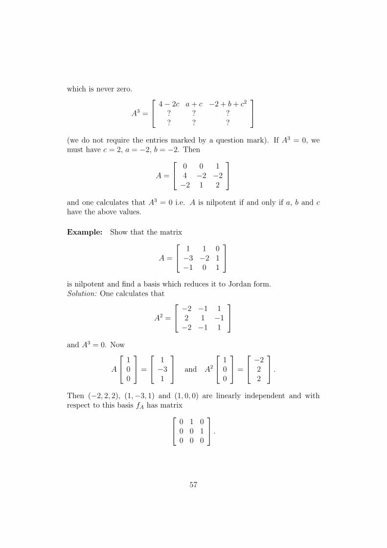
which is never zero.
A3 =
4− 2c a + c −2 + b+ c2
? ? ?? ? ?
(we do not require the entries marked by a question mark). If A3 = 0, wemust have c = 2, a = −2, b = −2. Then
A =
0 0 14 −2 −2−2 1 2
and one calculates that A3 = 0 i.e. A is nilpotent if and only if a, b and chave the above values.
Example: Show that the matrix
A =
1 1 0−3 −2 1−1 0 1
is nilpotent and find a basis which reduces it to Jordan form.Solution: One calculates that
A2 =
−2 −1 12 1 −1−2 −1 1
and A3 = 0. Now
A
100
=
1−31
and A2
100
=
−222
.
Then (−2, 2, 2), (1,−3, 1) and (1, 0, 0) are linearly independent and withrespect to this basis fA has matrix
0 1 00 0 10 0 0
.
57

Example: Calculate the minimal polynomials of
A =
1 1 10 1 10 0 1
B =
1 1 11 1 11 1 1
.
Solution: χA(λ) = (1− λ)3 and
(A− λI) =
0 1 10 0 10 0 0
.
It is clear that (A−I)2 6= 0 and (A−I)3 = 0 i.e. mA(λ) = (1−λ)3. χB(λ) =λ2(3− λ) and one calculates that B(B − 3I) = 0 i.e. mB(λ) = λ(3− λ).
Exercises: 1) For which values of a, b and c are the following matricesnilpotent?
A =
2 −2 a2 −2 b1 −1 0
B =
0 a b6 −3 c−2 1 −3
.
2) For each eigenvalue λ of the matrices A and B below calculate the valueof r for which Ker (A− λI)r becomes stationary:
A =
4 6 0−1 −1 00 0 1
B =
1 0 0 02 1 0 03 2 1 04 3 2 1
.
3) Solve the differential equations:
df
dt= g
dg
dt= −6f + 5g.
4) Diagonalise the matrix
A =
1 −1 2−1 1 22 2 −2
58
and use it to solve the difference equations:
an+1 = an − bn + 2cnbn+1 = −an + bn + 2cncn+1 = 2an + 2bn − 2cn
resp. the system of equations:
dx
dt= x − y + 2z
dy
dt= −x + y + 2z
dz
dt= 2x + 2y − 2z.
5) Let V1 be a subspace of the vector space V which is invariant under theoperator f ∈ L(V ). Show that if f is diagonalisable, then so is the restrictionof f to V1.6) A cyclic element for an operator f ∈ L(V ) is a vector x so that
{x, f(x), f 2(x), . . . , fn−1(x)}
forms a basis for V (where n = dimV ). Show that if f is diagonalisable,then it has a cyclic element if and only if its eigenvalues are distinct.7) Show that if two matrices are diagonalised by the same invertible matrix,then they commute.8) Let A be a diagonalisable n× n matrix. Show that a matrix B commuteswith every matrix that commutes with A if and only if there is a polynomialp so that B = p(A). Show that if A has distinct eigenvalues, then it sufficesfor this that B commutes with A.9) Let f ∈ L(V ) be such that each vector x ∈ V is an eigenvalue. Show thatthere is a λ ∈ R so that f = λId.10) Let f, g ∈ L(V ) commute. Show that each eigenspace of f is g-invariant.11) Suppose that f ∈ L(V ) has n distinct eigenvalues where n = dim V .Show that V contains precisely 2n f -invariant subspaces.12) Show that f ∈ L(V ) is nilpotent if and only if its characteristic polyno-mial has the form ±λn where n = dimV . Deduce that if f is nilpotent, thenfn = 0. 13) A nilpotent operator f on an n dimensional space V is nilcyclicif and only if V has a basis of the form (x, f(x), f 2(x), . . . , fn−1(x)) for somex ∈ V (i.e. x is a cyclic vector as defined in Exercise 6). Show that this isequivalent to each of the following conditions:
• fn = 0 but fn−1 6= 0;
59
• r(f) = n− 1;
• dimKer f = 1;
• there is no decomposition V = V1 ⊕ V2 where V1 and V2 are non-trivialsubspaces which are f -invariant.
14) Show that if A is an invertible n× n matrix, then
χA−1(λ) = (−1)nλn
detAχA(
1
λ).
Show that in general (i.e. without the condition on invertibility of A) wehave
tr (λI − A)−1 =χ′A(λ)
χA(λ)
whenever λ is not an eigenvalue of A.15) Show that if A is a nilpotent n × n matrix with Ak = 0, then I − A isinvertible and
(I −A)−1 = I + A+ · · ·+ Ak−1.
16) Let A be a complex 2 × 2 matrix which is not a multiple of the unitmatrix. Show that any matrix which commutes with A can be written in theform λI + µA (λ, µ ∈ C).17) Find a Jordan canonical form for the operator
D : Pol (n) → Pol (n).
18) Show that every n×n matrix over C can be represented as a sum D+NwhereD is a diagonalisable matrix, N is nilpotent and N and D commute.Show that there is only one such representation.19) A linear mapping f : V → V has an upper triangular representation(i.e. a basis with respect to which its matrix is upper triangular) if andonly if there is a sequence (Vi) of subspaces of V (i = 0, . . . , n) where thedimensional if Vi is i and Vi ⊂ Vi+1 for each i so that f(Vi) ⊂ Vi for eachi. Show directly (i.e. without using the Jordan canonical form) that sucha sequence exists (for operators on complex vector spaces) and use this togive a proof of the Cayley-Hamilton theorem independent of the existence ofa Jordan form. Show that if f and V are real, then such a representationexists if and only if χf has n real zeroes.20) Show that if A is an n × n matrix with eigenvalues λ1, . . . , λn then theeigenvalues of p(A) are p(λ1), . . . , p(λn).21) Let J be a Jordan block of the form Jn(λ). Calculate
60
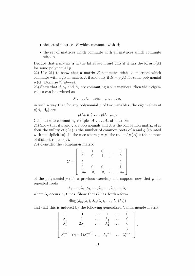
• the set of matrices B which commute with A;
• the set of matrices which commute with all matrices which commutewith A.
Deduce that a matrix is in the latter set if and only if it has the form p(A)for some polynomial p.22) Use 21) to show that a matrix B commutes with all matrices whichcommute with a given matrix A if and only if B = p(A) for some polynomialp (cf. Exercise 7) above).23) Show that if A1 and A2 are commuting n× n matrices, then their eigen-values can be ordered as
λ1, . . . , λn resp. µ1, . . . , µn
in such a way that for any polynomial p of two variables, the eigenvalues ofp(A1, A2) are
p(λ1, µ1), . . . , p(λn, µn).
Generalise to commuting r-tuples A1, . . . , Ar of matrices.24) Show that if p and q are polynomials and A is the companion matrix of p,then the nullity of q(A) is the number of common roots of p and q (countedwith multiplicities). In the case where q = p′, the rank of p′(A) is the numberof distinct roots of A.25) Consider the companion matrix
C =
0 1 0 . . . 00 0 1 . . . 0...
...0 0 0 . . . 1
−a0 −a1 −a2 . . . −a0
of the polynomial p (cf. a previous exercise) and suppose now that p hasrepeated roots
λ1, . . . , λ1, λ2, . . . , λi, . . . , λr, . . . , λr
where λi occurs ni times. Show that C has Jordan form
diag (Jn1(λ1), Jn2(λ2), . . . , Jnr(λr))
and that this is induced by the following generalised Vandermonde matrix:
1 0 . . . 1 . . . 0λ1 1 . . . λ2 . . . 0λ21 2λ1 . . . λ22 . . . 0...
...λn−11 (n− 1)λn−2
1 . . . λn−12 . . . λn−nr
r
.
61

(The first n1 columns are obtained by successive differentiation of the firstone and so on).
62

3.4 Functions of matrices and operators
We have often used the fact that we can substitute square matrices intopolynomials. For many applications, it is desirable to be able to do thisfor more general functions and we discuss briefly some of the possibilities.Suppose firstly that A is a diagonal matrix, say
A = diag (λ1, . . . , λn).
Then if we recall that for a polynomial p,
p(A) = diag (p(λ1), . . . , p(λn))
it is natural to define x(A) to be diag (x(λ1), . . . , x(λn)) for a suitable functionx. In order for this to make sense, it suffices that the domain of definition of xcontain the set {λ1, . . . , λn} of eigenvalues of A. In view of the importance ofthe latter set in what follows, we denote it by σ(A). It is called the spectrumof A. Of course, substitution satisfies the rules that (x+y)(A) = x(A)+y(A)and (xy)(A) = x(A)y(A).
If A is diagonalisable, say
S−1AS = D = diag (a,1 , . . . , λn),
we define x(A) to be
S · x(D) · S−1 = S · diag (x(λ1), . . . , x(λn)) · S−1.
The case where A is not diagonalisable turns out to be rather more tricky.Firstly, we note that it suffices to be able to define x(A) for Jordan blocks.For if A has Jordan form
S−1AS = diag (J1, . . . , Jr)
then we can define x(A) to be
S · diag (x(J1), . . . , x(Jr)) · S−1
once we know how to define the x(Ji). (We are using the notation diag (J1, . . . , Jr)for the representation of a Jordan form as a blocked diagonal matrix).
In order to motivate the general definition, consider the case of the squareroot of the Jordan matrix Jn(λ). Firstly, we remark that for λ = 0, no suchsquare root exists. We show this for the simplest case (n = 2) but the sameargument works in general.
63
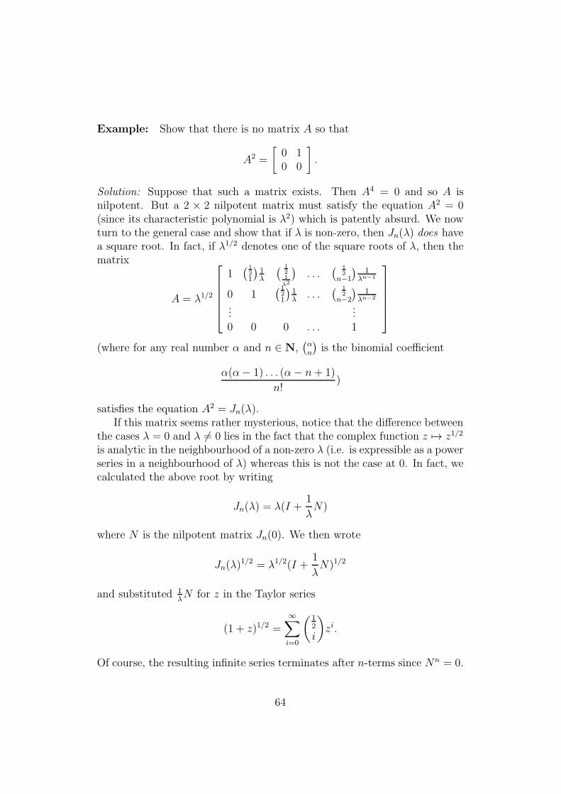
Example: Show that there is no matrix A so that
A2 =
[0 10 0
].
Solution: Suppose that such a matrix exists. Then A4 = 0 and so A isnilpotent. But a 2 × 2 nilpotent matrix must satisfy the equation A2 = 0(since its characteristic polynomial is λ2) which is patently absurd. We nowturn to the general case and show that if λ is non-zero, then Jn(λ) does havea square root. In fact, if λ1/2 denotes one of the square roots of λ, then thematrix
A = λ1/2
1( 1
21
)1λ
( 121λ2
). . .
( 12
n−1
)1
λn−1
0 1( 1
21
)1λ
. . .( 1
2n−2
)1
λn−2
......
0 0 0 . . . 1
(where for any real number α and n ∈ N,(αn
)is the binomial coefficient
α(α− 1) . . . (α− n+ 1)
n!)
satisfies the equation A2 = Jn(λ).If this matrix seems rather mysterious, notice that the difference between
the cases λ = 0 and λ 6= 0 lies in the fact that the complex function z 7→ z1/2
is analytic in the neighbourhood of a non-zero λ (i.e. is expressible as a powerseries in a neighbourhood of λ) whereas this is not the case at 0. In fact, wecalculated the above root by writing
Jn(λ) = λ(I +1
λN)
where N is the nilpotent matrix Jn(0). We then wrote
Jn(λ)1/2 = λ1/2(I +
1
λN)1/2
and substituted 1λN for z in the Taylor series
(1 + z)1/2 =∞∑
i=0
(12
i
)zi.
Of course, the resulting infinite series terminates after n-terms since Nn = 0.
64
If we apply the same method to the Taylor series
(1 + z)−1 = 1− z + z2 − z3 + . . .
then we can calculate the inverse of Jn(λ) for λ 6= 0. The reader can checkthat the result coincides with that given above.
This suggest the following method for defining x(A) where, for the sakeof simplicity, we shall assume that x is entire. This will ensure that x has aTaylor expansion around each λ in the spectrum of A. As noted above, weuse the Jordan form
S−1AS = diag (J1, . . . , Jr)
where Ji is Jni(λi). We define x(Ji) as follows. x has the Taylor expansion
x(λ) = x(λi) + x′(λi)(λ− λi) + . . .
around λi. If we substitute formally we get the expression
x(Ji) = x(λi)I + x′(λi)N + · · ·+ x(n−1)(λi)
(n− 1)!Nn−1
where Ji = λiI +N (i.e. N = Jni(0)).
We now give a purely algebraic form of the definition. Suppose that A isan n×n matrix with distinct eigenvalues λ1, . . . , λr and minimal polynomial
m(λ) =∏
(λ− λi)m1 .
We shall define x(A) for functions x which are defined on a neighbourhoodof the set of eigenvalues of A and have derivatives up to order mi − 1 at λifor each i. It is clear that there is a polynomial p so that
p(k)(λi) = x(k)(λi)
for each i and k ≤ mi − 1.Perhaps the easiest way to do this is as follows. Firstly we construct a
polynomial Lik (of minimal degree) which vanishes, together with its deriva-tives up to order mj − 1 at λj (j 6= i) and is such that the k-th derivative atλi is one, while all other ones vanish there (up to order mi − 1). We denotethis polynomial by Lik (it can easily be written down explicitly but as weshall not require this directly we leave its computation as an exercise for thereader).
Then the polynomial which we require is
p =∑
i,k
xikLik
65
where xik = x(k)(λi). Hence if we write Pik for the operator Lik(A), then
x(A) =∑
i,k
xikPik.
The Pik are called the components of A.In the special case where A has n distinct eigenvalues, then χA has the
form(λ− λ1) . . . (λ− λn).
The only relevant L’s are the Li0’s which we denote simply by Li. Thus Li
is the Lagrange interpolating polynomial
∏
j 6=i
λ− λjλk − λj
which takes on the value 1 at λi and the value 0 at the other λ’s. We note alsothe fact that the sum of the Li’s is the constant function one and that L2
i = Li
(both of these when the functions are evaluated at the eigenvalues). In thiscase, the components Pi = Li(A) satisfy the equations P 2
i = Pi (i.e. theyare projections) and their sum is the identity operator. The most importantexample of such a function of a matrix is the exponential function. Since thelatter is entire, we can substitute any matrix and we denote the result byexp(A) or eA. We note some of its simple properties:
• if A is diagonalisable, say A = SDS−1 where D = diag (λ1, . . . , λn),then
expA = S · diag (eλ1 , . . . , eλn) · S−1;
• if A = D + N where D is diagonalisable and N is nilpotent, bothcommuting, then expA = expD · expN and
expN =
∞∑
k=0
Nk
k!
where the series breaks off after finitely many terms;
• expA · exp(−A) = I (and so expA is always invertible);
• if (λ1, . . . , λn) are the eigenvalues of A, then (eλ1 , . . . , eλn) are the eigen-values of expA;
• if A and B commute, then so do expA and expB and we have theformula
exp(A+B) = expA · expB.In particular, if s, t ∈ R, then exp(s+ t)A = exp sA · exp tB;
66

• the function t 7→ exp tA from R into the set of n × n matrices isdifferentiable and
d
dt(exp tA) = A · exp(tA).
We remark that the statement in (6) means that the elements of the matrixexp tA, as functions of t, are differentiable. The derivative on the left handside is then the matrix obtained by differentiating its elements.
This property is particularly important since it means that the generalsolution of the system
dX
dt= AX
of differential equations where X is the column matrix
X(t) =
x1(t)...
xin(t)
whose elements are smooth functions is given by the formula
X(t) = exp tA ·X0
where X0 is the column matrixx1(0)...
xn(0)
of initial conditions.
Example: Consider the general linear ordinary differential equation of de-gree n
x(n) + an−1x(n−1) + · · ·+ a0x = 0
with constant coefficients. We can write this equation in the form
dX
dt= AX
where X is the column vector
x(t)x′(t)...
x(n−1)(t)
67

and A is the companion matrix
A =
0 1 0 . . . 00 0 1 . . . 0...
...0 0 0 . . . 1
−a0 −a1 −a2 . . . −an−1
of the polynomialp(t) = tn + an−1t
n−1 + · · ·+ a0.
As we know, the characteristic polynomial of this matrix is p and so itseigenvalues are the roots λ1, . . . , λn of p.
We suppose that these λi are all distinct. Then A is diagonalisable andthe diagonalising matrix is the Vandermonde matrix
V (λ1, . . . , λn) =
1 . . . 1λ1 . . . λn...
...λn−11 . . . λn−1
n
.
Hence if we write S for this matrix, we have
expAt = S · diag (eλ1t, . . . , eλnt) · S−1
and the solution of the above equation can be read off from the formula
X(t) = S · (eλ1t, . . . , eλnt) · S1X0
where X0 is the column matrix of initial values
x(0)x′(0)...
x(n−1)(0)
.
The reader can check that this provides the classical solution.In principle, the case of repeated roots for p can be treated similarly.
Instead of the above diagonalisation, we use the reduction of A to its Jordanform. The details form one of the main topics in most elementary books ondifferential equations.
68
Exercises: 1) Calculate expA where
A =
0 1 02 0 20 1 0
A =
[cos θ − sin θsin θ cos θ
]A =
[cos θ sin θsin θ − cos θ
]A =
[0 t−t 0
].
2) Solve the following system of differential equations:
dx1dt
= x1 − 12x3 + e−3t
dx2dt
= −x1 + 7x2 − 20x3dx3dt
= x1 + 5x3 + cos t.
3) If
C =
0 1 0 . . . 00 0 1 . . . 0...
...0 0 0 . . . 11 0 0 . . . 0
.
calculate exp tC.4) Calculate expA where A is the matrix of the differentiation operator Don Pol (n).5) Show that if A is an n × n matrix all of whose entries are positive, thenthe same holds for expA.6) Show that det(expA) = exp(trA).7) Show that the general solution of the equation
dX
dt= AX +B
with initial condition X(0) = X0, where A is a constant n× n matrix and Bis a continuous mapping from R into the space of n× 1 column matrices, isgiven by the equation
X(t) =
∫ t
0
exp((t− s)A)B(s) ds+ exp tA ·X0.
8) Show that if A is an n×n matrix with distinct eigenvalues λ1, . . . , λr andminimal polynomial
m(λ) =∏
(λ− λi)mi ,
69
then two polynomials p and q agree on A (i.e. are such that p(A) = q(A)) ifand only if for each i
p(λi) = q(λi) p′(λi) = q′(λi) . . . pmi−1(λi) = qmi−1(λi).
9) Let A and B be n × n matrices and define a matrix function X(t) asfollows:
X(t) = eAtCBBt.
Show that X is a solution of the differential equation
dX
dt= AX +XB
with initial condition X(0) = C.Deduce that if the integral
Y = −∫ ∞
0
eAtCeBt dt
converges for given matrices A, B and C, then it is a solution of the equation
AY + Y B = C.
10) Let A and B be n×n matrices which commute and suppose that A2 = A.Show that M(s) = AeBs is a solution of the functional equation M(s + t) =M(s)M(t). Show that if, on the other hand, M is a smooth function whichsatisfies this equation, then M(s) has the form AeBs where A = M(0) andB =M ′(0).11) For which matrices A are the following expressions defined:
sinA, cosA, tanA, sinhA, coshA, tanhA, ln(I + A)?
Show how to use the methods of this section to solve a differential equationof the form
d2X
dt2= AX
with initial values X(0) = X0, X′(0) = Y0. 12) Show that if a function x is
such that x(A) is defined, then so is x(At) and we have
x(At) = x(A)t.
13) Show that if A and B are commuting n× n matrices, then
x(B) = x(A) + x′(A) · (B − A) + · · ·+ x(m)(A) · (B − A)m
m!
for suitable functions x and integers m.
70

3.5 Circulants and geometry
An n× n matrix A is a circulant if it has the form
a0 a1 . . . an−1
an−1 a0 . . . an−2...
...a1 a2 . . . a)
.
Note that this just means that A is a polynomial function of the specialcirculant
C =
0 1 0 . . . 00 0 1 . . . 0...
...1 0 0 . . . 0
.
In fact, A is then p(C) where
p(t) = a0 + a1t+ · · ·+ an−1tn−1.
The following result gives an alternative characterisation of circulant matri-ces. It can be verified by direct calculation.
Proposition 19 An n × n matrix is circulant if and only if it commuteswith C.
We have already calculated the eigenvalues of C and found them to be
1, ω, ω2, . . . , ωn−1
where ω is the primitive root cos 2πn+ i sin 2π
n. The eigenvector corresponding
to ωk is easily seen to be uk = 1√n(ωk, ω2k, . . . , ωnk). (The reason for the
factor 1√nwill become apparent later). These eigenvectors are particularly
interesting since they are also eigenvectors for all polynomial functions of Ci.e. for the circulant matrices.
Here we shall discuss briefly the circulants of the form
A =
1 1 1 . . . 1 0 . . . 00 1 1 . . . 1 1 . . . 0...
...1 1 1 . . . 0 0 . . . 1
where there are m “ones” in each row. In other words,
A = p(C) where p(t) =1
m(1 + t+ · · ·+ tm−1).
71

It follows from the above that the eigenvalues of A are λ1, . . . , λn whereλn = 1 and
λk =1
m
1− ωkm
1− ωk
for k 6= n.Then we see immediately
• that A is invertible if and only if m and n are relatively prime;
• that if d is the greatest common divisor of m and n, then the dimensionof the kernel of fA is d and it has a basis consisting of the vectors
1
n(ωjd, ω2jd, . . . , 1, ωjd, . . . )
for 1 ≤ j ≤ d− 1.
These results have the following geometrical interpretation. Suppose that Pis an n-gon in R2. If we identify the points of R2 with complex numbers, wecan specify P by an n-tuple (z1, . . . , zn) of complex numbers (its vertices).For example, the standard square corresponds to the 4-tuple (o, 1, 1 + i, i).An n × n matrix A can be regarded as acting on such polynomials by leftmultiplication of the corresponding column matrix i.e. we define the polygonQ = A(P) to be the one with vertices ζ1, . . . , ζn where
ζ1...ζn
= A
z1...zn
.
Consider the transformation with matrix
A =1
m
1 1 . . . 1 0 . . . 10 1 . . . 1 1 . . . 0...
...1 1 . . . 1 0 . . . 1
discussed above. In this case, Q is the polygon whose vertices are the cen-troids of the vertices P1, . . . , Pm resp. P2, . . . , Pm+1 and so on. This polygonis called the m-descendant of P.
The results on the matrix A that we obtained above can now be expressedgeometrically as follows:
Ifm and n are relatively prime, then every polygonQ is them-descendantof a unique polygon P.
A more delicate investigation of the case where the greatest commonfactor d of m and n is greater than 1 leads to a characterisation of thosepolygons P which are m descendants (see the Exercises below).
72

Exercises: 1) Show that the determinant of the circulant matrix circ (a0, . . . , an−1)is
n−1∏
j=0
n−1∑
k=0
ωikak
where ω is the primitive n-th root of unity.2) A matrix A is called r-circulant if CA = ACr where C is the circulantmatrix of the text. Characterise such matrices directly and show that if A isr-circulant and B s-circulant, then AB is rs-circulant.3) Describe those matrices which are polynomial functions of the matrixJn(0).4) Suppose that the greatest common factor d of m and n is greater than 1.Identify the kernel and the range of the matrix
A =1
m
1 1 . . . 1 0 . . . 00 1 . . . 1 1 . . . 0...
...1 1 . . . 1 0 . . . 1
and use this to give a characterisation of those polygons which arem-descendantsresp. whose m-descendants are the trivial polygon with all vertices at theorigin.5) Diagonalise the following circulant matrices:
• circ (a, a+ h, . . . , a+ (n− 1)h);
• circ (a, ah, . . . , ahn−1);
• circ (0, 1, 0, 1, . . . , 0, 1).
6) Show that if A is a circulant matrix and x is a suitable function, thenx(A) is also a circulant.
73

3.6 The group inverse and the Drazin inverse
As a further application of the Jordan form we shall construct two specialtypes of generalised inverse for linear mappings (resp. matrices). These areof some importance in certain applications. The method will be the same inboth cases. Firstly we construct the inverse for matrices in Jordan form andthen use this to deal with the general case. We begin with the group inverse.A group inverse for an n× n matrix A is an n× n matrix S so that
ASA = A SAS = S
and A and S commute. As a simple example, suppose that A is the diagonalmatrix
diag (λ1, . . . , λr, 0, . . . , 0).
Then S = diag ( 1λ1, . . . , 1
λr, 0, . . . , 0) is obviously a group inverse for A. Hence
every diagonalisable matrix has a group inverse. (If A = P−1AP is diagonaland S is a group inverse for A as above, then S = P SP−1 is a group inversefor A).
More generally, note that if the vector space has the splitting
V = f(V )⊕Ker f
then we can use this to define a generalised inverse g = P ◦ f−1 where P isthe projection onto f(V ) along Ker f and f is the isomorphism induced by fon f(V ). In this case, g is easily seen to be a group inverse for f . Note thatfrom the analysis of section 3 of the present chapter, f has such a splittingin the case where r(f) = r(f 2). In terms of the Jordan form this meansthat the block corresponding to the zero eigenvalues is the zero block i.e. theJordan form is
diag (J1(λ1), . . . , Jr(λr), 0, . . . , 0)
where λ1, . . . , λr are the non-zero eigenvalues. The group inverse is then
diag (J1(λ1)−1, . . . , Jr(λr)
−1, 0, . . . , 0).
In terms of the minimal polynomial, this means that the matrix has a groupinverse provided the latter has the form
mA(λ) = λǫ(λ1 − λ)n1 . . . (λr − λ)nr
where ǫ is either 0 or 1.
74

The Drazin inverse A Drazin inverse for an n× n matrix A is an n× nmatrix S so that
• SAS = S;
• S and A commute;
• λ ∈ σ(A) if and only if λ† ∈ σ(S) where λ† = 1λfor λ 6= 0 and λ† = 0
for λ = 0;
• Ak+1S = Ak for some positive integer k.
Suppose first that A is a Jordan block Jn(λ). Then we define S to be Jn(λ)−1
if λ is non-zero and to be 0 if λ = 0. Then S satisfies the above four condition(with k = n if λ = 0). We denote this S by AD. Now if A has Jordan form
diag (A1, A2, . . . , Ar)
where each Ai is a Jordan block, we define AD to be the matrix
diag (AD1 , . . . , A
Dr ).
Once again, this satisfies the above four condition (this time with the integerk the maximum of the orders (ki) of the individual blocks corresponding tothe zero eigenvalue).
For a general matrix A we choose an invertible P so that A = P−1APwhere A has Jordan form. Then we define AD to be P−1ADP . Of course,AD is a Drazin inverse for A.
In terms of operators, the Drazin inverse can be described as follows:suppose that f : V → V is a linear transformation. Then, as we have seen,there is a smallest integer p at which the sequences
V ⊃ f(V ) ⊃ f 2(V ) ⊃ . . .
andKer f ⊂ Ker (f 2) ⊂ Ker(f 3) ⊂ . . .
become stationary. This integer is called the index of f and we have thesplitting
V = f p(V )⊕Ker (f p).
f , restricted to f p(V ), is an isomorphism of this space onto itself. Theoperator fD is that one which is obtained by composing the inverse of thelatter with the projection onto f p(V ) along Ker (f p).
75

Exercises: 1) For f ∈ L(V ) we define A(f) = f(V ) ∩Ker f . Show that
• dimA(f) = r(f)− r(f 2);
• Ker f ⊂ f(V ) if and only if r(f) = r(f 2) − n(f) where n(f) =dimKer f ;
• f(V ) = Ker f if and only if f 2 = 0 and n(f) = r(f);
• V = f(V )⊕Ker f if and only if lr(f) = r(f 2).
2) Show that the Drazin inverse is uniquely determined i.e. that there is atmost one matrix S so that SAS = S, AS = SA and Ak+1S = Ak for somepositive integer k.3) Show that the group inverse is uniquely determined i.e. there is at mostone matrix S so that ASA = A, SAS = S and AS = SA.4) Show that if f ∈ L(V ) has a Drazin inverse fD, then fD(V ) = f(V ),Ker fD = Ker(fk) and ffD = fDf is the projection onto f(V ) along Ker fk.5) The following exercise shows how the existence of the Drazin inverse canbe deduced directly from the existence of the minimal polynomial, withoutusing the Jordan form. Suppose that mA has the form
t 7→ aktk + · · ·+ tr
where tk is the lowest power of t which occurs with non-vanishing coefficient(we can suppose that k ≥ 1). The equation mA(A) = 0 can then be writtenin the form
Ak = Ak+1B
where B is a suitable polynomial in A. Show that Ak+rBr = Ak for eachr ≥ 1 and deduce that S = AkBk+1 satisfies the defining conditions forthe Drazin inverse. 6) Show that if A is an n × n matrix, then there is apolynomial p so that AD = p(A).
76
4 EUCLIDEAN ANDHERMITIAN SPACES
4.1 Euclidean space
In chapter II we saw that a number of basic geometrical concepts could bedefined in terms of the scalar product. We now discuss such products inhigher dimensions where, in the spirit of chapter III, we use the axiomaticapproach. We shall prove higher dimensional versions of many of the resultsof chapter II, culminating in the spectral theorem for self-adjoint operators.
Definition: A scalar product (or inner product) on a real vector spaceV is a mapping from V × V → R, denoted as
(x, y) 7→ (x|y)
so that
• the mapping is bilinear i.e.
(λ1x1+λ2x2|µ1y1+µ2y2) = λ1µ1(x1|y1)+λ1µ2(x1|y2)+λ2µ1(x2|y1)+λ2µ2(x2|y2)
for λ1, λ2, µ1, µ2 ∈ R, x1, x2, y1, y2 ∈ V ;
• it is symmetric i.e. (x|y) = (y|x) (x, y ∈ V );
• it is positive definite i.e. (x|x) > 0 if x 6= 0.
Property (3) implies the following further property:(4) if x ∈ V is such that (x|y) = 0 for each y ∈ V , then x = 0. (Choose
y = x in (3)).A euclidean vector space is a (real) vector space V together with a
scalar product.Of course, a vector space can be provided with many distinct scalar prod-
ucts. This can be visualised inR2 where a scalar product is given by a bilinearform of the type
(x, y) 7→2∑
i,j
aijξiηj
and the positive definiteness means exactly that the corresponding conicsection
2∑
i,j
aijξiξj = 1
77

is an ellipse. Hence the choice of a scalar product in R2 is just the choice ofan ellipse with centre 0.
The standard euclidean space is Rn with the scalar product
(x|y) =∑
i
ξiηi.
Another example is the space Pol (n) with the scalar product
(p|q) =∫ 1
0
p(t)q(t) dt.
The latter is a subspace of the infinite dimensional space C([0, 1]) with scalarproduct
(x|y) =∫ 1
0
x(t)y(t) dt.
Using the scalar product we can define the length (or norm) of a vectorx—written ‖x‖. It is defined by the formula
‖x‖ =√(x|x).
We then define the distance between two points x, y in V to be ‖x − y‖,the length of their difference. As in R2 and R3 there is a close connectionbetween the concepts of norm and scalar product. Of course, the norm isdefined in terms of the latter. On the other hand, the scalar product can beexpressed in terms of the norm as follows:
‖x+ y‖2 = (x+ y|x+ y) = (x|x) + 2(x|y) + (y|y)
and so
(x|y) = 1
2(‖x+ y‖2 − ‖x‖2 − ‖y‖2).
As in R2 the norm and scalar product satisfy the Cauchy-Schwartz in-equality:
|(x|y)| ≤ ‖x‖‖y‖ (x, y ∈ V ).
This is named after the discoverers of the classical case
ξ1η1 + · · ·+ ξnηn ≤ (ξ21 + · · ·+ ξn)12 (η21 + · · ·+ η2n)
12 .
To prove the general inequality, we consider the quadratic function
T 7→ (x+ ty|x+ ty) = t2‖y‖2 + 2t(x|y) + ‖x‖2
78
which is non-negative by the positive-definiteness of the product. Hence itsdiscriminant is less than or equal to zero i.e. 4(x|y)2−4(‖x‖2‖y‖2) ≤ 0 whichreduces to the required inequality. (Note that the same proof shows that theCauchy-Schwarz inequality is strict i.e. |(x|y)| < ‖x‖‖y‖ unless x and y areproportional. For the above quadratic is strictly positive if x and y are notproportional and then the discriminant must be negative).
From this we can deduce the triangle inequality
‖x+ y‖ ≤ ‖x‖ + ‖y‖.
For
‖x+ y‖2 = (x+ y|x+ y)
= ‖x‖2 + 2(x|y) + ‖y‖2≤ ‖x‖2 + 2‖x‖‖y‖+ ‖y‖2= (‖x‖+ ‖y‖)2.
From the Cauchy-Schwarz inequality we see that if x and y are non-zero thenthe quotient
(x|y)‖x‖‖y‖
lies between −1 and 1. Hence there is a unique θ ∈ [0, π] so that
cos θ =(x|y)‖x‖‖y‖ .
θ is called the angle between x and y.We can also define the concept of orthogonality or perpendicularity: two
vectors are perpendicular (written x ⊥ y if (x|y) = 0.As in R2 and R3 we use this notion to define a special class of bases:
Definition: An orthogonal basis in V is a sequence (x1, . . . , xn) of non-zero vectors so that (xi|xj) = 0 for i 6= j. If, in addition, each vector hasunit length, then the system is orthonormal.
An orthogonal system is automatically linearly independent. For if
λ1x1 + . . . λmxm = 0,
then0 = (λ1ξ1 + · · ·+ λmxm|xi) = λi(xi|xi)
and so λi = 0 for each i.
79
Hence an orthonormal system (x1, . . . , xn) with n elements in an n-dimensionalspace is a basis and such bases are called orthonormal bases. The classicalexample is the canonical basis (e1, . . . , en) for R
n.One advantage of an orthonormal basis is the fact that the coefficient of
a vector with respect to the basis can be calculated simply by taking scalarproducts. In fact x =
∑nk=1(x|xk)xk. (This is sometimes called the Fourier
series of x). This is proved by a calculation similar to the one above. Also ifx =
∑ni+1 λixi and y =
∑nk=1 µkxm, then
(x|y) = (
n∑
i=1
λixi|n∑
k=1
µkxk) =
n∑
i,k=1
λiµk(xi|xk) =n∑
i=1
λiµi
and, in particular, ‖x‖ =√λ21 + · · ·+ λ2n. Thus the scalar product and norm
can be calculated from the coordinates with respect to an orthonormal basisexactly as we calculate them in Rn.
Every euclidean space has an orthonormal basis and to prove this we usea construction which has a natural geometrical background and which wehave already used in dimensions 2 and 3.
Proposition 20 If V is an n-dimensional euclidean space, then V has anorthonormal basis (x1, . . . , xn).
Proof. We construct the basis recursively. For x1 we take any unit vector.If we have constructed x1, . . . , xr we construct xr+1 as follows. We take anyz which does not lie in the span of x1, . . . , xr (of course, if there is no suchelement we have already constructed a basis). Then define
xr+1 = z −r∑
i=1
(z|xi)xi.
xr+1 is non-zero and is perpendicular to each xi (1 ≤ i ≤ r). Hence if we put
xr+1 =xr+1
‖xr+1‖
then (xr, . . . , xr+1) is an orthonormal system.The proof actually yields the following result:
Proposition 21 Every orthonormal system (x1, . . . , xr) in V can be ex-tended to an orthonormal basis i.e. there exist elements xr+1, . . . , xn so that(x1, . . . , xn) is an orthonormal basis for V .
80
The standard way to construct an orthonormal basis is called the Gram-Schmid process and consists in applying the above method in connectionwith a given basis (y1, . . . , yn), using y1 for x1 and, at the r-th step usingyr+1 for z. This produces an orthonormal basis x1, . . . , xn of the form
x1 = b11y1
x2 = b21y1 + b22y2...
xn = bn1y1 + · · ·+ bnnyn
where the diagonal elements bii are non-zero. If we apply this method to thecase where the space is Rn (identified with the space of row vectors) and thebasis (y1, . . . , yn) consists of the rows of an invertible n × n matrix A, weobtain a lower triangular matrix
B =
b11 0 . . . 0b21 b22 . . . 0...
...bn1 bn2 . . . bnn
and a matrix Q whose rows form an orthonormal basis for Rn (such matricesare called orthonormal) so that Q = BA. Since B is invertible and itsinverse L is also a lower triangular matrix, we obtain the following result onmatrices:
Proposition 22 Any n× n invertible matrix A has a representation of theform A = LQ where Q is an orthonormal matrix and L is lower triangular.
We can use this fact to prove a famous inequality for the determinant ofthe n× n matrix. We have
| detA| ≤∏
i
(∑
j
|aij|2)12
(i.e. the determinant is bounded by the product of the euclidean norms ofthe columns. This is known as Hadamard’s inequality).Proof. We can write the above equation as L = AQt. Hence
lii =∑
j
aijqij ≤ (∑
j
a2ij)12 (∑
j
q2ij)12
the last step using the Cauchy-Schwarz inequality. Hence (since∑
j q2ij = 1),
| detA| = | detLU | = | detL| =∏
i
|lii| ≤∏
i
(∑
j
a2ij
)1/2
81

(We have used the fact that if the matrix U is orthonormal, then its deter-minant is ±1. This follows as in the 2-dimensional case from the equationU tU = I—see below).
In the context of euclidean space, those linear mapping which preservedistance (i.e. are such that ‖f(x)‖ = ‖x‖ for x ∈ V ) are of particular interest.As in the two and three dimensional cases, we can make the following simpleremarks (note that we only consider linear isometries):I. If f is an isometry, then f preserves scalar products i.e. (f(x)|f(y)) = (x|y)(x, y ∈ V ). For
(f(x)|f(y)) = 1
2(‖f(x+ y)‖2 − ‖f(x)‖2 − ‖f(y)‖2)
=1
2(‖x+ y‖2 − ‖x‖2 − ‖y‖2)
= (x|y).
On the other hand, this property implies that f is an isometry. (Take x = y).II. An isometry from V into V1 is automatically injective and so is surjectiveif and only if dimV = dim V1. In particular, any isometry of V into itself isa bijection.III. An isometry maps orthonormal systems onto orthonormal systems. Inparticular, if dimV = dimV1, then f maps orthonormal bases onto orthonor-mal bases. On the other hand, if f maps one orthonormal basis (x1, . . . , xn)onto an orthonormal system (y1, . . . , yn) in V1, then f is an isometry. For ifx =
∑k λkxk, then f(x) =
∑k λkyk and so
‖f(x)‖2 =∑
k
λ2k = ‖x‖2.
IV. By this criterium, if A is an n × n matrix, then since fA maps thecanonical basis for Rn onto the columns of A, we see that fA is an isometryif and only if the columns of A form an orthonormal basis. This can beconveniently expressed in the equation At ·A = I (or equivalently, At = A−1
or A · At = I). Matrices with this property are called orthonormal as wenoted above.
Typical isometries in Rn are reflections i.e. operators with matrices ofthe form
1 0 0 . . . 0 00 1 0 . . . 0 0...
...0 0 0 . . . 1 00 0 0 . . . 0 −1
82

with respect to some orthonormal basis and rotations i.e. those with ma-trices of the form
1 0 0 . . . 0 00 1 0 . . . 0 0...
...0 0 0 . . . cos θ − sin θ0 0 0 . . . sin θ cos θ
with respect to some orthonormal basis.
Example: Show that the mapping
(A|B) = tr (ABt)
is a scalar product on Mn.Solution: The bilinearity and symmetry:
(A1 + A2|B) = tr((A1 + A2)Bt)
= tr (A1Bt + A2B
t)
= tr(A1Bt) + tr (A2B
t)
= (A1|B) + (A2|B).
(A|B) = tr (ABt)
= tr(ABt)t
= tr(BAt)
= (B|A).
Positive definiteness:
(A|A) = tr (AAt) =∑
i,j
a2ij > 0
for A 6= 0.We remark that the basis (eij : i, j = 1, . . . , n) is then orthonormal where
eij is the matrix with a 1 in the (i, j)-th position and zeroes elsewhere.
Example: Show that the mapping
(x|y) = 4ξ1η1 − 2ξ1η2 − 2ξ2η1 + 3ξ2η2
83
is a scalar product on R2.Solution: The matrix of the quadratic form is
[4 −2−2 3
]
with eigenvalues the roots of λ2 − 7λ+ 8 which are positive.We calculate an orthonormal basis with respect to this scalar product by
applying the Gram-Schmidt process to x1 = (1, 0), x2 = (0, 1). This gives
e1 =x1
‖x1‖= (
1
2, 0);
y2 = (0, 1)− ((0, 1)|(12, 0))(
1
2, 0) =
1
2, 1);
e2 =1√2(2, 1).
Example: Construct an orthonormal basis for Pol (2) with scalar product
(p|q) =∫ 1
0
p(t)q(t) dt
by applying the Gram-Schmidt method to (1, t, t2).Solution:
x0 = 1, x0 = 1;
x1(t) = t− (t|1)1 = t = −1
2;
x1(t) =√12(t− 1
2);
x2(t) = t2 − (t2|x0)x0(t)− (t2|x1)x1(t)
= t2 − t +1
6;
x2(t) = 6√5(t2 − t+
1
6).
We calculate the Fourier series of 1 + t + t2 with respect to this basis. Wehave
λ1 =
∫ 1
0
(t2 + t+ 1) dt =11
6
λ2 =√12
∫ 1
0
(t2 + t + 1)(t− 1
2) dt =
1√3
λ3 = 6√5
∫ 1
0
(t2 + t + 1)(t2 − t+1
6) dt =
1
6√5
84
and so
t2 + t + 1 =11
6+ 2(t− 1
2) + (t2 − t+
1
6).
Example If (e1, . . . , en) is an orthonormal basis for V and x1, . . . , xn ∈ V ,then
det
(x1|e1) . . . (x1|en)...
...(xn|e1) . . . (xn|en)
2
= det
(x1|x1) . . . (x1|xn)...
...(xn|x1) . . . (xn|xn)
.
(And hence the right hand side is non-negative and vanishes if and only ifthe xi are linearly dependent).Solution: This follows from the equalities
(xi|xj) =n∑
k=1
(xi|ek)(xj |ek)
which can be written in the matrix form
(x1|e1) . . . (x1|en)...
...(xn|e1) . . . (xn|en)
(x1|e1) . . . (x1|en)...
...(xn|e1) . . . (xn|en)
=
(x1|x1) . . . (x1|xn)...
...(xn|x1) . . . (xn|xn)
.
Exercises: 1)
• Apply the Gram-Schmidt process to obtain an orthonormal systemfrom the following sets:
(1, 0, 1), (2, 1,−1), (−1, 1, 0) in R3;
(1, 2, 1, 2), (1, 1, 1, 0), (2, 1, 0, 1) in R4.
• Calculate the orthogonal projection of (1, 3,−2) on [(2, 1, 3), (2, 0, 5)].
2) Show that if the ai are positive, then
(
n∑
i=1
ai)(
n∑
i+1
1
ai) ≥ n2
(n∑
i=1
ai)2 ≤ n(
n∑
i=1
a2i ).
85
3) If x1, . . . , xm are points in Rn, then the set of points which are equidistantfrom x1, . . . , xm is an affine subspace which is of dimension n −m if the xiare affinely independent.4) Let (x0, . . . , xn) be affinely independent points inRn. Then there is exactlyone hypersphere through these points and its equation is
det
1 1 . . . 1X0 X1 . . . X...
...(x0|x0) (x1|x1) . . . (x|x)
= 0
where X is the column vector corresponding to x etc.5) Suppose that a1, . . . , an, b1, . . . , bn are positive numbers. Show that either
a1b1
+ · · ·+ anbn
≥ n
orb1a1
+ · · ·+ bnan
≥ n.
6) Show that a sequence (x1, . . . , xn) in a euclidean space V is an orthogonalbasis if an only if for each x ∈ V ,
‖x‖2 =n∑
i=1
|(x|xi)|2.
7) Calculate an orthonormal basis of polynomials for Pol (3) by applyingthe Gram-Schmidt process to the basis (1, t, t2, t3) with respect to the scalarproduct
(p|q) =∫ ∞
0
p(t)q(t)e−t dt.
8) Let pn be the polynomial
dn
dtn(t2 − 1)n.
Show that ∫ 1
−1
tkpn(t) dt = 0 (k < n)
and hence that the system (pn) is orthogonal for the corresponding scalarproduct. (This shows that the system (pn) is, up to norming factors, thesequence obtained by applying the Gram-Schmidt process to the sequence(tn). These functions are called the Legendre polynomials).
86

9) Approximate sin x by a polynomial of degree 3 using the orthonormalbasis of the last exercise. Use this to check the accuracy by calculating anapproximate value of sin 1. 10) Show that for an n×n matrix A the followinginequality holds:
n∑
i,j=1
a2ij ≥1
n(trA)2.
For which matrices do we have equality?11) Show that if (ξi) and (ηi) are vectors in Rn, then
(∑
i
ξ2i )(∑
i
η2i ) = (∑
i
ξiηi)2 −
∑
1≤i<j≤n
(ξiηj − ξjηi)2.
(This is a quantitative version of the Cauchy-Schwarz equations).12) Consider the euclidean spaceMn with the scalar product discussed in theexample abovje. If A is an n × n matrix one can apply the Gram-Schmidtprocess to the sequence I, A,A2, A
3, . . . . This will stop at the smallest kso that Ak is a linear combination of the earlier. This provides a specificdescription of the minimal polynomial of A. The reader is invited to fill inthe details.13) Let (x1, . . . , xk) be a linearly independent set in the euclidean space V .Show that if x ∈ V , then its orthogonal projection x0 onto the linear span ofthe above vectors is given by the formula
x0 =
k∑
r+1
λrxr
where λj =detGj
detG. Here G is the matrix [gij] where gij = (xi|xj) and Gj is
the matrix obtained from G by replacing the j-th column by ??14) Show that if x1, . . . , xn is a basis for the euclidean space V , then theGram-Schmidt process, applied to this basis, leads to the system (yk) where
yk = (dk−1dk)12D
where dn = detG (G as in 13)) and
Dn = det
(x1|x1) . . . (x1|xn)...
...(xn−1|x1) . . . (xn−1|xn)
x1 . . . xn
.
87

(The last expression is to be understood as the linear combination of the x’sobtained by formally expanding the “determinant” along the last row).15) Use Hadamard’s inequality to show that
| detA|2 ≤ Kn · nn2
where A is an n× n matrix and K = maxi,j |aij|.16) Show that
min
∫ ∞
0
e−t(1 + a1t + . . . antn)2 dt =
1
n + 1;
min
∫ 1
0
(1 + a1t+ · · ·+ antn)2 dt =
1
(n+ 1)2
where the minima are each taken over the possible choices of the coefficientsa1, . . . , an.
88
4.2 Orthogonal decompositions
In our discussion of vector spaces we saw that each subspace has a com-plementary subspace which determines a splitting of the original space. Ingeneral this complementary subspace is not unique but, as we shall now see,the structure of a euclidean space allows us to choose a unique one in anatural way.
Definition: If V1 is a subspace of the euclidean space V , then the set
V ⊥1 = {x ∈ V : (x|y) = 0 for each y ∈ V1}
of vectors which are orthogonal to each vector in V1 forms a subspace of Vcalled the orthogonal complement of V1.
Proposition 23 V1 and V ⊥1 are complementary subspaces. More precisely,
if (x1, . . . , xn) is an orthonormal basis for V so that V1 = [x1, . . . , xr], thenV ⊥1 = [xr+1, . . . , xn]. Hence V = V1 ⊕ V ⊥
1 .
Proof. It suffices to check that y =∑n
i+1 λixi is orthogonal to each xi(i = 1, . . . , r) and so to V1 if and only if λ − i = 0 for i = 1, . . . , r i.e.y ∈ [xr+1, . . . , xn].
We shall write V = V ⊥ V1 to denote the fact that V = V1 ⊕ V2 andV1 ⊥ V2.
If V = V1 ⊥ V2 and (x1, . . . , xn) is an orthonormal basis with V1 =[x1, . . . , xr], then
PV1(x) =r∑
r=1
(x|xi)xi
is the projection of x onto V1 along V ⊥1 . It is called the orthogonal pro-
jection of x onto V1 and has the following important geometric property:PV1(x) is the nearest point to x in V1 i.e.
‖x− PV1(x)‖ < ‖x− z‖ (z ∈ V1, z 6= PV1(x)).
For if z ∈ V1, we have
‖x− z‖2 = ‖x− PV1(x)‖2 + ‖PV1(x)− z‖2
since x− PV1(x) ⊥ PV1(z).The point x− 2PV1(x) is then the mirror image (or reflection) of x in
V ⊥1 . The linear mapping Id− 2PV1 is called a reflection.
89
In the same way we define an orthogonal decomposition
V = V1 ⊥ · · · ⊥ Vr.
This means that V = V1 ⊕ · · · ⊕ Vr and Vi ⊥ Vj (i.e. x ⊥ y if x ∈ Vi, y ∈ Vj)when i 6= j.
Then if Pi is the orthogonal projection onto Vi,
• P1 + · · ·+ Pr = Id;
• PiPj = 0 (i 6= j).
Such a sequence of projections is called a partition of unity.Orthogonal splittings of the space are obtained by partitioning an or-
thonormal basis (x1, . . . , xn) i.e. we define Vi to be [xki−1, . . . , xki−1] where
1 = k0 < k1 < · · · < kr = n+ 1.On the other hand, if we have such a splitting V1 ⊥ · · · ⊥ Vr, then we
can construct an orthonormal basis for V by combining orthonormal basesfor the components V1, . . . , Vn.
Exercise: 1) Consider the space Mn with the scalar product
(A|B) = tr (BtA).
Show that Mn is the orthogonal direct sum of the symmetric and the anti-symmetric matrices.
90

4.3 Self-ajdoint mappings— the spectral theorem
One of the most important consequences of the existence of a scalar productis that the fact that it induces a certain symmetry on the linear operatorson the space. If f : V → V1 we say that g : V1 → V is ajdoint to f if(f(x)|y) = (x|g(y)) for x ∈ V and y ∈ V1. We shall presently see that sucha g always exists. Furthermore it is unique. The general construction isillustrated by the following two examples:I. Consider the mapping f : R2 → R2 defined by the matrix
[a11 a12a22 a22
].
A simple calculation shows that
(f(x)|y) = a11ξ1η1 + a12ξ2η1 + a21ξ1η2 + a22ξ2η2.
If g is the mapping with matrix At, then analogously
(x|g(y)) = a11η1ξ1 + a21η2ξ1 + a12η1ξ2 + a22η2ξ2
and both are equal.II. Now consider the mapping f : Rn → Rm defined by the matrix A = [aij ].We know that aij is the i-th coordinate of f(ej) i.e. that aij = (f(ej)|ei) (re-member the method of calculating coordinates with respect to an orthonor-mal basis). Hence if a mapping g : Rm → Rn exists which is adjoint to f ,then
aij = (f(ej)|ei) = (ej|g(ei))and by the same reasoning the latter is the (j, i)-th entry of g. In otherwords the only possible choice for g is the mapping with matrix B = At. Asimple calculation shows that this mapping does in fact satisfy the requiredconditions. Since these considerations are perfectly general, we state andprove them in the form of the following Proposition:
Proposition 24 If f : V → V1 is a linear mapping there is exactly onelinear mapping g : V1 → V which is adjoint to f . If f has matrix A withrespect to orthonormal bases (xi) resp. (yj) then g is the mapping with matrixAt with respect to (yj) and (xi).
91
Proof. Suppose that x ∈ V and y ∈ V1. Then
(f(x)|y)) = (f(n∑
j=1
(x|xj)xj)|m∑
k=1
(y|yk)yk)
= (
m∑
i−1
(
n∑
j=1
aij(x|xj)yi|∑
(y|yk)yk)
=m∑
i=1
n∑
j=1
m∑
k=1
aij(x|xj)(y|yk)(yi|yk)
=
m∑
i=1
n∑
j=1
aij(x|xj)(y|yi).
Similarly, we have
(x|g(y)) =m∑
i=1
n∑
j=1
aij(x|xj)(y|yi)
if g is the operator with matrix as in the formulation and so
(f(x)|y) = (x|g(y))
i.e. g is adjoint to f .Naturally, we shall denote g by f t and note the following simple properties:
• (f + g)t = f t + gt;
• (λf)t = λf t;
• (fg)t = gtf t;
• (f t)t = f ;
• an operator f is an isometry if and only if f tf = Id. In particular, ifV = V1, this means that f t = f−1.
We prove the last statement. We have seen that f is an isometry if and onlyif (f(x)|f(y)) = (x|y) for each x, y and this can be restated in the form
(f tf(x)|y) = (x|y)
i.e. f tf = Id.A mapping f : V → V is said to be self-adjoint if f t = f i.e.
(f(x)|y) = (x|f(y))
92

for x, y ∈ V . This is equivalent to f being represented by a symmetric Awith respect to an orthonormal basis. In particular, this will be the case iff is represented by a diagonal matrix. The most important result of thischapter is the following which states that the converse is true:
Proposition 25 Let f : V → V be self-adjoint. Then V possesses an or-thonormal basis consisting of eigenvectors of f . With respect to this basis, fis represented by the diagonal matrix diag (λ1, . . . , λn) where the λi are theeigenvalues of f .
In terms of matrices this can be stated in the following form:
Proposition 26 Let A be a symmetric n × n matrix. Then there exists anorthonormal matrix U and real numbers λ1, . . . , λn so that
U tAU = U−1AU = diag (λ1, . . . , λn).
In particular, a symmetric matrix is diagonalisable and its characteristic poly-nomial has n real roots.
This follows immediately from the above Proposition, since the transfer ma-trix between orthonormal bases is orthonormal.
Before proceeding with the proof we recall that we have essentially provedthis result in the two dimensional case in our treatment of conic sections inChapter II.
One of the consequences of the result is the fact that every symmetricmatrix A has at least one eigenvalue. Indeed this is the essential part ofthe proof as we shall see and before proving this we reconsider the two di-
mensional case. The symmetric matrix
[a11 a12a12 a22
]induces the quadratic
formφ1(x) = (fA(x)|x)
and so define the conic section
Q1 = {x : φ1(x) = 1}.
If we compare this to the form φ2(x) = (x|x) which defines the unit circlesQ2 = {x : φ2(x) = 1} and consider the case where Q1 is an ellipse, then wesee that the eigenvectors of A are just the major and minor axes of the ellipse
and these can be characterised as those directions x for which the ratioφ1(x)
φ2(x)is extremal. Hence we can reduce the search for eigenvalues to one for theextremal value of a suitable functional, a problem which we can solve with
93
the help of elementary calculus. This simple idea will allow us to prove thefollowing result which is the core of the proof. We use the Proposition thata continuous function on a closed, bounded subset of Rn is bounded andattains its supremum.
Proposition 27 Lemma Let f : V → V be self-adjoint. Then there existsan x ∈ V with ‖x‖ = 1 and λ ∈ R so that f(x) = λx (i.e. f has aneigenvalue).
Proof. We first consider the case where V = Rn with the natural scalarproduct. Then f is defined by an n × n symmetric matrix A. Consider thefunction
φ : x 7→ (f(x)|x)(x|x)
on V \ {0}. Then φ(λx) = φ(x) for λ 6= 0. There exists an x1 ∈ V sothat ‖x1‖ = 1 and φ(x1) ≥ φ(x) for x ∈ V with ‖x‖ = 1. Hence, by thehomogeneity,
φ(x1) ≥ φ(x) (x ∈ V \ {0}).We show that x1 is an eigenvector with f(x1) = λ1x1 where λ1 = φ(x1) =(f(x1)|x1). To do this choose y 6= 0 in V . The function
ψ : t 7→ φ(x1 + ty)
has a minimum for t = 0. We show that ψ′(x) exists and its value is2(z|f(x1))− 2(y|x1)λ1. Hence this must vanish for each y i.e.
(y|f(x1)− λ1x1) = 0.
Since this holds for each y, f(x1) = λ1x1. To calculate the derivative of ψwe compute the limit as t tends to zero of the difference quotient
1
t(ψ(t)− ψ(0)) =
1
t(φ(x1 + ty)− φ(x1)).
But this is the limit of the expression
1
t[(x1|x1)[(f(x1)|x1) + 2t(f(x1)|y)) + t2(f(y)|y)]− (f(x1)|x1)[(x1|x1) + 2t(x1|y) + t2(y|y)]
(x1 + ty|x1 + ty)(x1|x1)]
which is easily seen to be
2(y|f(x1))− 2(y|x1)λ1.In order to prove the general case (i.e. where f is an operator on an
abstract euclidean space), we consider an orthonormal basis (x1, . . . , xn) forV and let A be the matrix of f with respect to this basis. Then A has aneigenvalue and of course this means that f also has one.
We can now continue to the proof of the main result:
94

Proof. The proof is an induction argument on the dimension of V . Fordim V = 1, the result is trivial (all 1 × 1 matrices are diagonal!) The stepn− 1 → n: By the Lemma, there exists an eigenvector x1 with ‖x1‖ = 1 andeigenvalue λ1. Put V1 = {x1}⊥ = {x ∈ V : (x|x1) = 0}. Then V1 is (n− 1)-dimensional and f(V1) ⊂ V1 since if x ∈ V1, then (f(x)|x1) = (x|f(x1)) =(x|λ1x1) = 0 and so f(x) ∈ V1. Hence by the induction hypothesis thereexists an orthonormal basis (x2, . . . , xn) consisting of eigenvectors for f . Then(x1, . . . , xn) is the required orthonormal basis for V .
The above proof implies the following useful characterisation of the largestresp. smallest eigenvalue of f ;
Corollar 3 Let f : V → V be a self-adjoint linear mapping with eigenvaluesλ1, . . . , λn numbered so that λ1 ≤ · · · ≤ λn. Then
λ1 = min{φ(x) : x ∈ V \ {0}}λn = max{φ(x) : x ∈ V \ {0}}.
This can be generalised to the following so-called minimax characterisationof the k-th eigenvalue:
λk = minmax{(f(x)|x) : x ∈ V \ {0}, (x|y1) = · · · = (x|yr) = 0}the minimum being taken over all finite sequences y1, . . . , yr of unit vectorswhere r = n− k.
We remark here that it follows from the proofs of the above results that iff is such that (f(x)|x) ≥ 0 for each x in V , then its eigenvalues are all non-negative (and they are positive if (f(x)|x) > 0 for non-zero x). Such f arecalled positive semi-definite resp. positive definite and will be examinedin some detail below. It follows form the above minimax description of theeigenvalues that
λk(f + g) ≥ λk(f)
whenever f is self-adjoint and g is positive semi-definite (with strict inequalitywhen g is positive definite). As we have seen, a symmetric operator is alwaysdiagonalisable. Using this fact, we can prove the following weaker result forarbitrary linear operators between euclidean spaces.
Proposition 28 Let f : V → V1 be a linear mapping. Then there exist or-thonormal bases (x1, . . . , xn) for V and (y1, . . . , ym) for V1 so that the matrixof f with respect to these bases has the form
[A1 00 0
]
where A1 = diag (µ1, . . . , µr), r is the rank of f and µ1, . . . , µr are positivescalars.
95

The corresponding result for matrices is the following:
Proposition 29 If A is an m× n matrix then there exist orthonormal ma-trices U1 and U2 so that U1AU2 has the above form.
Proof. We prove the operator form of the result. Note that the mappingf tf on V is self-adjoint since (f tf)t = f tf tt = f tf . We can thus choosean orthonormal basis (xi) consisting of eigenvectors for f tf . If λi is thecorresponding eigenvalue we can number the xi so that the first r eigenvaluesare non-zero but the following ones all vanish. Then each λi is positive(i = 1, . . . , r) and ‖f(xi)‖ =
√λi. For
λi = λi(xi|xi) = (λixi|xi) = (f tf(xi)|xi) = (f(xi)|f(xi)) > 0.
Also if i 6= j then f(xi) and f(xj) are perpendicular since
(f(xi)|f(xj)) = (f tf(xi)|xj) = λi(xi|xj) = 0.
Hence if we put
y1 =f(x1)√λ1
, . . . , yr =f(xr)√λr
then (y1, . . . , yr) is an orthonormal system in V1. We extend it to an or-thonormal basis (y1, . . . , ym) for V1. The matrix of f with respect to thesebases clearly has the desired form.
The proof shows that the µi are the square roots of the eigenvalues of ftf
and so are uniquely determined by f . They are call the singular values off .
Example: Let V be a euclidean space with a basis (xi) which is not as-sumed to be orthonormal. Show that if f ∈ L(V ) has matrix A with re-spect to this basis, then f is self-adjoint if and only if AtG = GA whereG = [(xi|xj)]i,j.Solution: f is self-adjoint if and only if
(f(n∑
i=1
λixi|n∑
j=1
µjxj))) = (n∑
i=1
λixi|f(n∑
j=1
µjxj))))
for all choices of scalars λ1, . . . , λn, µ1, . . . , µn and this holds if and only if
(f(xi)|xj) = (xi|f(xj))
for each i and j. Substituting the values of f(xi) and f(xj) one gets therequired equation AtG = GA.
96

Exercises: 1) Calculate the adjoints of the following operators:
• (ξ1, ξ2, ξ3) 7→ (ξ1 + ξ2 + ξ3, ξ1 + 2ξ2 + 2ξ3, ξ1 − 2ξ2 − 2ξ3) (on R3 withthe usual scalar product);
• the differentiation operator D on Pol (n);
• p 7→ (t 7→ tp(t)) from Pol (n) into Pol (n+ 1).
2) Show that if f ∈ L(V ), then
Ker f t = f(V )⊥ f t(V ) = (Ker f)⊥.
3) Show that for every self-adjoint operator f there are orthogonal projectionsP1, . . . , Pr and real scalars λ1, . . . , λr so that
• PiPj = 0 if i 6= j;
• P1 + · · ·+ Pr = Id;
• f = λ1P1 + · · ·+ λrPr.
Calculate the Pi explicitly for the operator on R3 with matrix
0 1 01 0 10 1 0
.
4) Show that an operator f is an orthogonal projection if and only if f 2 = fand f is self-adjoint. Let f be a self-adjoint operator so that fm = fn fordistinct positive integers m and n. Show that f is an orthogonal projection.5) Show that if f is an invertible, self-adjoint operator, then λ is an eigenvalueof f if and only if 1
λis an eigenvalue of f−1. Show that f and f−1 have the
same eigenvectors.
97
4.4 Conic sections
As mentioned above, the theory of conic sections in the plane was the mainsource of the ideas which lie behind the spectral theorem. We now indicatebriefly how the latter can be used to give a complete classification of higherdimensional conic sections. The latter are defined as follows:
Definition: A conic section in a euclidean space V is a set of the form
Q = {x ∈ V : (f(x)|x) + 2(b|x) + c = 0}
where b ∈ V , c ∈ R and f is a self-adjoint operator on V . In order to simplifythe analysis we assume that the conic section is central i.e. has a point ofcentral symmetry (for example, in R2 an ellipse is central whereas a parabolais not). If we then take this point to be the origin, it follows that x ∈ Q ifand only if −x ∈ Q. Analytically this means that b = 0 i.e. A has the form
{x ∈ V ; (f(x)|x) + c = 0}.
Proposition 30 If Q is a conic section of the above form, then there is anorthonormal basis (x1, . . . , xn) for V and real numbers λ1, . . . , λn so that
Q = {x = ξ1x1 + . . . ξnxn : λ1ξ21 + . . . λnξ
2n + c = 0}.
This result can be restated as follows: let f be the isometry from V into Rn
which maps (x‘1, . . . , xn) onto the canonical basis (e1, . . . , en). Then
f(Q) = {(ξ1, . . . , ξn) ∈ Rn : λ1ξ21 + · · ·+ λnξ
2n + c = 0}.
Proof. Choose for (x1, . . . , xn) an orthonormal basis for V so that f(xi) =λixi. Then
(f(x)|x) = λ1ξ21 + · · ·+ λnξ
2n
if x = ξ1x1 + . . . ξnxn.As an application, we classify the central conics in R3. Up to an isometry
they have the form
{(ξ1, ξ2, ξ3) : λ1ξ21 + λ2ξ22 + λ3ξ
23 + c = 0}.
By distinguishing the various possibilities for the signs of the λ’s, we obtainthe following types: λ1, λ2, λ3 all positive. Then we can reduce to the form
ξ21a2
+ξ22b2
+ξ23c2
+ d = 0
98

and this is an ellipsoid for d < 0, a point for d = 0 and the empty set for d > 0.λ1, λ2, λ3 all negative. This can be reduced to the first case by multiplyingby −1. λ1, λ2 positive, λ3 negative. Then we can write the equation in theform
ξ21a2
+ξ22b2
− ξ23c2
+ d = 0.
(the cases λ1, λ3 > 0, λ2 < 0 resp. λ2, λ3 > 0, λ1 < 0 can be reduced to theabove by permuting the unknowns). The above equation represents a circularcone (d = 0) or a one-sheeted or two sheeted hyperboloid (depending on thesign of d). The cases where at least one of the λ’s vanishes can be reducedto the two-dimensional case.
Exercises: 1) Show that each non-central conic
{x ∈ R3 : (f(x)|x) + 2(g|x) + c = 0}
where b 6= 0 is isometric to one of the following:
{x :ξ21a2
+ξ22b2
− 2ξ3 + d = 0}
{x :ξ21a2
− ξ22b2
− 2ξ3 + d = 0}{x : ξ21 − 2x2 + d = 0}
and discuss their geometrical forms.2) If
Q = {x ∈ R3 :ξ21a2
+ξ22b2
+ξ23c2
= 1}
is an ellipsoid with a ≤ b ≤ c show that the number of planes through 0which cut Q in a circle is 1 (if a = b or b = c but a 6= c), 2 (if a, b, c aredistinct) or infinite (if a = b = c). 3) Diagonalise the quadratic form
φ(x) =n∑
i=1
(ξi − ξj)2
on Rn.
99
4.5 Hermitian spaces
For several reasons, it is useful to reconsider the theory developed in thischapter in the context of complex vector space. Amongst other advantagesthis will allow us to give a purely algebraic proof of the central result—thediagonalisation of symmetric matrices. This is because the existence of aneigenvalue in the complex case follows automatically from the fundamentaltheorem of algebra.
We begin by introducing the concept of a hermitian vector space i.e.a vector space V over C with a mapping
( | ) : V × V → C
so that
• (λx+ y|z) = λ(x|z) + (y|z) (linearity in the first variable);
• (x|x) ≥ 0 and (x|x) = 0 if and only if x = 0;
• (x|y) = (y|x) (x, y ∈ V ).
Examples: All the examples of euclidean spaces can be “complexified” inthe natural and obvious ways. Thus we have: a) the standard scalar product
((λ1, . . . , λn))|(µ1, . . . , µn)) = λ1µ1 + · · ·+ λnµn
on Cn;b) the scalar product
(p|q) =∫ 1
0
p(t)q(t) dt
on the space PolC(n) of polynomials with complex coefficients. Note therather unexpected appearance of the complex conjugation in condition 2)above. This means that the scalar product is no longer bilinear and is usedin order to ensure that condition 1) can hold. However, the product issesqui-linear (from the classical Greek for one and a half) i.e. satisfies thecondition
(n∑
i=1
λixi|n∑
j=1
µjyj) =n∑
i,j=1
λiµj(xi|yj).
All of the concepts which we have introduced for euclidean spaces can beemployed, with suitable changes usually necessitated by the sesquilinearityof the scalar product, for hermitian spaces. We shall review them briefly: Thelength of a vector x is ‖x‖ =
√(x|x). Once again we have the inequality
|(x|y)| ≤ ‖x‖‖y‖ (x, y ∈ V ).
100

(Since there is a slight twist in the argument we give the proof. Firstly wehave (for each t ∈ R),
0 ≤ (x+ ty|x+ ty) = ‖x‖2 + 2tℜ(x|y) + t2‖y‖2
and, as in the real case, this gives the inequality
ℜ(x|y) ≤ ‖x‖‖y‖.
Now there is a complex number λ with |λ| = 1 and λ(x|y) > 0. If we applythe above inequality with x replaced by λx we get
|(x|y)| = |(λx|y)| = λ(x|y) = ℜλ(x|y) = ℜ(λx|y) ≤ ‖λx‖‖y‖ = ‖x‖‖y‖.
Using this inequality, one proves just as before that the distance functionsatisfies the triangle inequality i.e.
‖x+ y‖ ≤ ‖x‖ + ‖y‖.
For reasons that we hope will be obvious we do not attempt to define theangle between two vectors in hermitian space but the concept of orthogonalitycontinues to play a central role. Thus we say that x and y are perpendicularif (x|y) = 0 (written x ⊥ y). Then we can define orthonormal systems andbases as before and the Gram-Schmidt method can be used to show that everyhermitian space V has an orthonormal basis (x1, . . . , xn) and the mapping
(λ1, λ2, . . . , λn) 7→ λ1x1 + · · ·+ λnxn
is an isometry from Cn onto V i.e. we have the formulae
(x|y) = λ1µ1 + · · ·+ λnµn
‖x‖2 = |λ1|2 + · · ·+ |λn|2
if x = λ1x1 + · · ·+ λnxn, y = µ1x1 + . . . µnxn.
Exercises: 1) Let f be the linear mapping on the two dimensional space
C2 with matrix A =
[a bc d
]. Then the scalar product on C2 defines a
norm there and so a norm for operators. Show that the norm of the aboveoperator is given by the formula
‖f‖2 = 1
2(h2 +
√[(h2 − 4| detA|2]).
101
(Calculate the singular values of A).2) Show that if H is a hermitian matrix of the form A+ iB where A and Bare real and A is non-singular, then we have the formula
(detH)2 = (detA)2 det(I + A−1BA−1B).
3) Show that if U is a complex n×n matrix of the form P + iQ where P andQ are real, then U is unitary (i.e. such that U∗U = I) if and only if P tQ issymmetric and P tP +QtQ = I.
102
4.6 The spectral theorem—complex version
If f ∈ L(V, V1) there is exactly one mapping g : V1 → V so that
(f(x)|y) = (x|g(y)) (x ∈ V, y ∈ V1).
We denote this mapping by f ∗. The proof is exactly the same as for the realcase, except that we use the formula
aij = (f(xj)|yi) = (xj |g(yj)) = (g(yi)|xj)
for the elements of the matrix A of f with respect to the orthonormal bases(x1, . . . , xn) resp. (y1, . . . , ym) to show that the matrix of f ∗ is A∗, the n×mmatrix obtained from A by taking the complex conjugates of elements andthen transposing.
The linear mapping f on V is hermitian if f ∗ = f i.e. if (f(x)|y) =(x|f(y)) (x, y ∈ V ). This means that the matrix A of f with respect toan orthonormal basis satisfies the condition A = A∗ (i.e. aij = aji for eachi, j). Such matrices are also called hermitian. f : V → V1 is unitaryif (f(x)|f(y)) = (x|y) (x, y ∈ V ). This is equivalent to the condition thatf ∗f = Id. Hence the matrix U of f (with respect to orthonormal bases) mustsatisfy the condition U∗U = I (i.e. the columns of U are an orthonormalsystem in Cn). If dimV = dimV1 (= n say), then U is an n× n matrix andthe above condition is equivalent to the equation U∗ = U−1. Such matricesare called unitary.
We now proceed to give a purely algebraic proof of the so-called spectraltheorem for hermitian operators. We begin with some preliminary results oneigenvalues and eigenvectors:
Lemma 1 If f ∈ L(V ) with eigenvalue λ, then
• λ is real if f is hermitian;
• |λ| = 1 if f is unitary.
Proof. 1) if the non-zero element x is a corresponding eigenvector, then wehave
(f(x)|x) = (λx|x) = λ(x|x)and
((f(x)|x) = (x|f(x)) = (x|λx) = λ(x|x)and so λ = λ. 2) Here we have
(x|x) = (f(x)|f(x)) = (λx|λx) = |λ|2(x|x)
and so ‖λ‖2 = 1.
103
Proposition 31 Lemma If λ1, λ2 are distinct eigenvalues of the hermitianmapping f with corresponding eigenvectors x1, x2, then x1 ⊥ x2.
Proof. We have (f(x1)|x2) = (x1|f(x2)) and so
(λ1x1|x2) = (x1|λ2x2) i.e. (λ1 − λ2)(x1|x2) = 0.
(Recall that λ2 = λ2 by the Lemma above). Hence (x1|x2) = 0.
Proposition 32 Lemma If f ∈ L(V ), then Ker f = Ker (f ∗f).
Proof. Clearly Ker f ⊂ Ker f ∗f . Now if x ∈ Ker f ∗f , then f ∗f(x) = 0 andso (f ∗f(x)|x) = 0 i.e. (f(x)|f(x)) = 0. Thus f(x) = 0 i.e. x ∈ Ker f .
In passing we note that this means that if A is an m × n matrix, thenr(A) = r(A∗A) = r(A∗).
Corollar 4 If f ∈ L(V ) is hermitian and r ∈ N, then Ker f = Ker f r.
Proof. Applying the last result repeatedly, we get the chain of equalities
Ker f = Ker f 2 = · · · = Ker f 2k = . . .
Each Ker f r lies between two terms of this series and so coincides with Ker f .We now come to our main result:
Proposition 33 If f ∈ L(V ) is a hermitian mapping, then there exists anorthonormal basis (xi) for V so that each xi is an eigenvector for f . Withrespect to this basis, f has the matrix diag (λ1, . . . , λn) where the λi are the(real) eigenvalues of f .
Proof. Let Vi = Ker (f−λiId). It follows from the above corollary (appliedto f − λ1Id) that V is the direct sum
V = V1 ⊕ Im(f − λ1Id).
(Recall from Chapter VII that we have such a splitting exactly when the ker-nel of a mapping coincides with the kernel of its square). A simple inductionargument shows that V is the direct sum
V = V1 ⊕ V2 ⊕ · · · ⊕ Vr.
However, we know, by the Lemma above that Vi ⊥ Vj if i 6= j and so in factwe have
V = V1 ⊥ · · · ⊥ Vr.
Hence we can construct the required basis by piecing together orthonormalbases for the various Vi.
104
Corollar 5 If A is a hermitian n × n matrix, then there exists a unitaryn× n matrix U and real numbers λ1, . . . , λn so that
U−1AU = diag (λ1, . . . , λn).
A useful sharpening of the spectral theorem is as follows:
Proposition 34 Let f and g be commuting hermitian operators on V . ThenV has an orthonormal basis (x1, . . . , xn) whereby the xi are simultaneouslyeigenvectors for f and g.
Proof. Let λ1, . . . , λr be the distinct eigenvalues of f and put Vi = Ker (f−λiId). Then g(Vi) ⊂ Vi. For if x ∈ Vi, then f(x) = λix and f(g(x)) =g(f(x)) = g(λix) = λig(x) i.e. g(x) ∈ Vi. Hence if we apply the aboveresult to g on Vi, we can find an orthonormal basis for the latter consistingof eigenvectors for g (regarded as an operator on Vi). Of course they arealso eigenvectors for f and so the basis that we get for V by piecing togetherthese sub-bases has the required properties.
For matrices, this means that if A and B are hermition n × n matrices,then there is a unitary matrix U so that both U∗AU and U ∗BU are diagonal(real) matrices.
Example: We diagonalise the matrix A =
[1 + i 11 1 + i
].
Solution: The characteristic polynomial is
(1 + i)2 − 2(1 + i)λ+ λ2 − 1
with roots 2 + i and i. The corresponding eigenvectors are 1√2(1,−1) and
1√2(1, 1). hence U∗AU = diag (i, 2 + i) where U = 1√
2
[1 1−1 1
].
Example: Show that if A is hermitian, then I + iA is invertible and U =(I − iA)(I + iA)−1 is unitary.Solution: We can diagonalise A as
V ∗AV = diag (λ1, . . . , λn)
where the λi are real. Then
V ∗AV = diag (1 + iλ1, . . . , 1 + iλn)
105

and the right hand side is invertible. Hence so is the left hand side. Thisimplies that (I + iA)−1 exists. Then
V ∗(I − iA)(I + iA)V = diag (1− iλ11 + iλ1
, . . . ,1− iλn1 + iλn
).
The right hand side is clearly unitary. Exercises: 1) Show that an operatorf on a hermitian space is an orthogonal projection if and only if f = f ∗f . 2)Let A be a complex n× n matrix, p a polynomial. Show that if p(A∗A) = 0,then p(AA∗) = 0.3) Let p be a complex polynomial in two variables. Show that if A is an n×ncomplex matrix so that p(A,A∗) = 0, then p(λ, λ) = 0 for any eigenvalueλ of A. What can you deduce about the eigenvalues of a matrix A whichsatisfies one of the conditions:
A∗ = cA (c ∈ R) A∗A = A∗ + A A∗A = −I?
4) Let A be an n× n complex matrix with eigenvector X and eigenvalue λ1.Show that there is a unitary matrix U so that U−1AU has the block form
λ1
B0
for some n× (n− 1) matrix B. Deduce that there is a unitary matrix U sothat U−1AU is upper triangular and that if A is hermitian, then the lattermatrix is diagonal. (This exercise provides an alternative proof of the spectraltheorem).
106

4.7 Normal operators
Normal operators are a generalisation of hermitian ones. Consider first thediagonal matrix
A = diag (λ1, . . . , λn).
A need not necessarily be hermitian (indeed this is the case precisely when theλi are real). However, it does satisfy the weaker condition that AA∗ = A∗Ai.e. that A and A∗ commute. We say that such A are normal. Similarly,an operator f on V is normal if f ∗f = ff ∗. Note that unitary mappingsare examples of normal mappings—they are not usually hermitian. We shallnow show that normal mappings have diagonal representations. In orderto do this, we note that any f ∈ L(V ) has a unique representation in theform f = g + ih where g and h are hermitian (compare the representationof a complex number z in the form x + iy with x and y real). Indeed iff = g+ ih, then f ∗ = g− ih and so f +f ∗ = 2g i.e. g = 1
2(f +f ∗). Similarly,
h =1
2i(f − f ∗). This proves the uniqueness. On the other hand, it is clear
that if g and h are as in the above formula, then they are hermitian andf = g + ih.
The fact that normal operators are diagonalisable will follow easily fromthe following simple characterisation: f is normal if and only if g and hcommute.Proof. Clearly, if g and h commute, then so do f = g+ ih and f ∗ = g− ih.On the other hand, if f and f ∗ commute then so do g and h since both arelinear combinations of f and f ∗.
Proposition 35 If f ∈ L(V ) is normal, then V has an orthonormal basis(x1, . . . , xn) consisting of eigenvectors of f .
Proof. We write f = g + ih as above and find an orthonormal basis(x1, . . . , xn) consisting of vectors which are simultaneously eigenvectors for gand h, say g(xi) = λixi, h(xi) = µixi. Then
f(xi) = g(xi) + ih(xi) = (λi + µi)(xi)
as claimed.
Corollar 6 If f ∈ L(V ) is unitary, then there exists an orthonormal ba-sis (x1, . . . , xn) so that the matrix of f has the form diag (eiθ1, . . . , eiθn) forsuitable θ1, . . . , θn ∈ R.
107

We close this section with the classification of the isometries of Rn. Thisgeneralises the results of Chapter II on those of R2 and R3. The methodwe use is a standard one for deducing results about the real case from thecomplex one and can also be employed to deduce the spectral theorem forself-adjoint operators on euclidean spaces from the corresponding one forhermitian operators.
We require the following simple Lemma:
Lemma 2 Let V be a subspace of Cn with the property that if z ∈ V , thenℜz and ℑz also belong to V (where if z = (z1, . . . , zn), then
ℜz = (ℜz1, . . . ,ℜzn) ℑz = (ℑz1, . . . ,ℑzn)).
Then V has an orthonormal basis consisting of real vectors (i.e. vectors zwith ℑz = 0.]
Proof. We consider the set of all real vectors in V . Then it follows fromthe assumptions that this is a euclidean space whose real dimension coincideswith the complex one of V . If (x1, . . . , xr) is an orthonormal basis for thisspace, it is also one for V .
Proposition 36 Let f be an isometry of the euclidean space V . Then thereis an orthonormal basis (x1, . . . , xn) for V with respect to which f has blockmatrix of the form
Ir 0 0 . . . 00 −Is 0 . . . 00 0 Dθ1 . . . 0
0 0...
...0 0 0 . . . Dθt
for suitable integers r, s, t with r + s+ 2t = n where Dθ denotes the matrix
[cos θ − sin θsin θ cos θ
].
Proof. Let A be the matrix of f with respect to an orthonormal basis. Weregard A as a unitary operator on Cn. Since its non-real eigenvalues occurin complex conjugate pairs there is a (complex) unitary matrix U so that
U−1AU = diag (1, 1, . . . , 1,−1, . . . ,−1, eiθ1 , e−iθ1, . . . , eiθt , e−iθt).
From this it follows that Cn splits into the direct sum
V1 ⊕ V−1 ⊕ (W1 ⊕W ′1)⊕ · · · ⊕ (Wt ⊕W ′
t )
108

where
V1 = {x : fA(x) = x}V−1 = {x : fA(x) = −x}Wi = {x : fA(x) = eiθix}W ′
i = {x : fA(x) = e−iθix}.
Now consider V1. Then since A is real, z ∈ V1 if and only if ℜz ∈ V1 andℑz ∈ V1. Hence by the Lemma above we can choose an orthonormal basis(x1, . . . , xr) for V1 consisting of real vectors. Similarly, we can construct anorthonormal basis for V−1 consisting of real vectors (y1, . . . , ys).
For the same reason, the mapping
z 7→ z = ℜz − ℑz
maps Wi onto W ′i . Hence if (z1, . . . , zt) is an orthonormal basis for Wi,
(z1, . . . , zt) is an orthonormal basis forW ′i . Now fA maps the two dimensional
space spanned by zi and zi into itself and has matrix
[eiθi 00 e−iθi
]
with respect to this basis.We introduce the real bases wi and w
′i where
wi =zi + zi√
2w′
i =zi − zi
i√2
and consider the mapping fA on the two dimensional real space spanned bythese vectors. Then a simple calculation shows that wi and w
′i are perpen-
dicular (since zi ⊥ zi) and that the matrix of fA with respect to this basisis [
cos θi − sin θisin θi cos θi
].
If we combine all the basis elements obtained in this way, we obtain anorthonormal basis of the required sort.
Exercises: 1) Show that if f is a linear operator on a hermitian spaceV , then either of the following conditions is equivalent to the fact that f isnormal:
• (f(x)|f(y)) = (f ∗(x)|f ∗(y)) (x, y ∈ V );
109
• ‖f(x)‖ = ‖f ∗(x)‖ (x ∈ V ).
2) Show that an m× n complex matrix has factorisations
A = UB = CV
where U (resp. V ) is unitary m×m (resp. n× n) and B and C are positivesemi-definite. Show that if A is normal (and so square), then U and B canbe chosen in such a way that they commute.3) Show that a complex n × n matrix A is normal if and only if there is acomplex polynomial p so that A∗ = p(A).4) Let A be a normal matrix and suppose that all of the row sums have acommon value c. Show that the same is true of the column sums. What isthe common value in this case?5) Let A be a normal n× n matrix. Show that the set of eigenvalues of A issymmetric about zero (i.e. is such that if λ is an eigenvalue then so is −λ) ifand only if trA2k+1 = 0 for k = 0, 1, 2, . . . .6) Let U be an isometry of the hermitian space V and put
V1 = {x : Ux = x}.
Show that if Un is the mapping
Un =1
n(I + U + · · ·+ Un−1)
then for each x ∈ V , Unx converges to the orthogonal projection of x ontoV1.7) If f ∈ L(V ) is such that f ∗ = −f , then Id + f is invertible and (Id −f)(Id + f)−1 is unitary. Which unitary operators can be expressed in thisform?8) Show that if an n × n complex matrix is simultaneously unitary andtriangular, then it is diagonal.9) Let A be a normal matrix with the property that distinct eigenvalueshave distinct absolute values. Show that if B is a normal matrix, then ABis normal if and only if AB = BA. (Note that it is not true in general thatAB is normal if and only if A and B commute (where A and B are normalmatrices) although the corresponding result holds for self-adjoint mappings.The above result implies that this is true in the special case where either Aor B is positive definite).10) Let f ∈ L(V ) be such that if x ⊥ y, then f(x) ⊥ f(y). Show that thereexists an isometry f and a λ ∈ R so that f = λg.11) (This exercise provides the basis for a direct proof of the spectral theoremfor isometries onRn without having recourse to the complex result). Suppose
110

that f is an orthonormal operator on Rn. Show that there exists a one- ortwo-dimensional subspace of Rn which is f -invariant. (One can suppose thatf has no eigenvalues. Choose a unit vector x so that the angle between xand f(x) is minimum. Show that if y is the bisector of the angle between
x and f(x) (i.e. y =x+ f(x)
2), then f(y) lies on the plane through x and
f(x)—hence the latter is f -invariant).
111

4.8 The Moore-Penrose inverse
We now return once again to the topic of generalised inverses. Recall that iff : V → W is a linear mapping, we construct a generalised inverse for f byconsidering splittings
V = V1 ⊕ V2 W = W1 ⊕W2
where V2 is the kernel of f , W1 the image and V1 and W2 are complementarysubspaces. In the absence of any further structure, there is no natural way tochoose W2 and V1. However, when V and W are euclidean space, the mostobvious choices are the orthogonal complements V1 = V ⊥
2 and W2 = W⊥1 .
Then generalised inverse that we obtain in this way is uniquely specified anddenoted by f †. It is called the Moore-Penrose inverse of f and has thefollowing properties:
• f †ff † = f †;
• ff †f = f †;
• f †f is the orthogonal projection onto V1 and so is self-adjoint;
• ff † is the orthogonal projection onto W1 and so is self-adjoint.
In fact, these properties characterise f †—it is the only linear mapping fromW into V which satisfies them as can easily be seen.
It follows that if y ∈ W , then x = f †(y) is the “best” solution of theequation f(x) = y in the sense that
‖f(x)− y‖ ≤ ‖f(z)− y‖
for each z ∈ V i.e. f(x) is the nearest point to y in f(V ). In addition x isthe element of smallest norm which is mapped onto this nearest point.
In terms of matrices, these results can be restated as follows: let V andWhave orthonormal bases (x1, . . . , xn) resp. (y1, . . . , ym) and let f have matrixA with respect to them. Then the matrix A† of f † satisfies the conditions:
AA†A = A A†AA† = A† AA† and A†A are self-adjoint.
Of course, A† is then called the Moore-Penrose inverse of A and isuniquely determined by the above equations. The existence of f † can alsobe proved elegantly by using the result on singular values from the thirdparagraph. Recall that we can choose orthonormal bases (x1, . . . , xn) resp.(y1, . . . , ym) so that the matrix of f has the block form
[A1 00 0
]
112

with A1 = diag (µ1, . . . , µr). Then f† is the operator with matrix
[A−1
1 00 0
]
with respect to (y1, . . . , ym) resp. (x1, . . . , xn). Note that f is injective if andonly if r = n. In this case, f has matrix
[A1
0
]
and f † is the mapping (f tf)−1f t as one can verify by computing the matrixof the latter product.
Of course, the abstract geometric description of the Moore-Penrose in-verse is of little help in calculating concrete examples and we mention someexplicit formulae which are often useful.
Firstly, suppose that A has block representation [B C] where B is aninvertible (and hence square) matrix. Then it follows from the results onpositive definite matrices that BBt + CCt is invertible. The Moore-Penroseinverse of A is then given by the formula
A† =
[Bt(BBt + CCt)−1
Ct(BBt + CCt)−1
]
as can be checked by multiplying out.
Example: Consider the matrix
A =
1 0 . . . 0 10 1 . . . 0 1...
...0 0 . . . 1 1
.
Then A is of the above form with B = In and one can easily calculate thatA† is the matrix
1
n + 1
n −1 −1 . . . −1−1 n −1 . . . −1...
...−1 −1 −1 . . . n1 1 1 . . . 1
The Moore-Penrose inverse can also be calculated by means of the fol-lowing recursion method. We put
B = A∗A
113
and define
C0 = I
C1 = tr (C0B)I − C0B
C2 =1
2tr (C1B)I − C1B
and so on. It turns out that CrB vanishes where r is the rank of A and theearlier values have non-vanishing trace. Then we have the formula
A† =(r − 1)Cr−1A
∗
tr (Cr−1B).
This can be checked by noting that the various steps are independent of thechoice of basis. Hence we can choose bases so that the matrix of the operatordefined by A has the form [
A1 00 0
]
where A1 = diag (λ1, . . . , λr). This is a simple calculation.As an application, we consider the problem of the least square fitting of
data. Let (t1, y1), . . . , (tn, yn) be points in R2. We determine real numbersc, d so that the line y = ct + d provides an optimal fit. This means that cand d should be a “solution” of the equation
t1 1...
...tn 1
[cd
]=
y1...yn
.
If we interpret this in the sense that c and d are to be chosen so that theerror
(y1 − ct1 − d1)2 + · · ·+ (yn − ctn − dn)
2
be as small as possible, then this reduces to calculating the Moore Penroseinverse of
A =
t1 1...
...tn 1
since the solution is[cd
]= A†
y1...yn
.
114

If the ti are distinct (which we tacitly assume), then A† is given by theformula
A† = (AtA)−1At.
In this case
AtA =
[ ∑t2i tt n
]
where t = t1 + · · ·+ tn.
Example: We consider the concrete case of the data
0 1 2 3 5
for the value of t and0 2 3 4 6
for the corresponding values of the y’s, then we have
A =
0 11 12 13 15 1
and so
AtA =
[39 1111 5
]
and
(AtA)−1 =1
74
[5 −11
−11 39
].
This leads to the solution
[cd
]=
1
74
[5 −11
−11 39
] [0 1 2 3 51 1 1 1 1
]
02345
=
[71745174
].
Similar applications of the Moore-Penrose inverse arise in the problem ofcurve fitting. Here one is interested in fitting lower order curves to givendata. In chapter V we saw how the methods of linear algebra could beapplied. In practical applications, however, the data will be overdeterminedand will not fit the required type of curve exactlyl. In this case, the Moore-Penrose inverse can be used to find a curve whcih provides what is, in acertain sense, a best fit. We illustrate this with an example.
115

Example: Suppose that we are given a set of points P1, . . . , Pn in the planeand are looking for an ellipse which passes through them. In order to simplifythe arithmetic, we shall assume that the ellipse has equation of the form
αξ21 + βξ22 = 1
(i.e. that the principal axes are on the coordinate axes). Then we are requredto find (positive) α and β so that the equations
α(ξi1)2 + β(ξi2)
2 = 1
are satisfied (where Pi has coordinates (ξi1, ξi2)). This is a linear equation
with matrix
A =
(ξ11)2 (ξ12)
2
......
(ξn1 )2 (ξn2 )
2
.
Our theory would lead us to expect that the vector
[a b
]= A†
1...1
will be a good solution.
Exercises: 1) Show that the least square solution of the system
x = bi (i = 1, . . . , n)
is the mean value of b1, . . . , bn.2) Calculate explicitly the least square solution of the system
yi = cit+ d
considered above.3) Suppose that f is an operator on the hermitian space V . Show that if f issurjective, then ff t is invertible and the Moore-Penrose inverse of f is givenby the formula
f † = f t(ff t)−1.
Interpret this in terms of matrices.4) Show that f ∈ L(V ) commutes with its Moore-Penrose inverse if and onlyif the ranges of f and f ∗ coincide and this is equivalent to the fact that wehave splitting
V = f(V ) ⊥ Ker (f)
116

resp. that there is an orthonormal basis with respect to which f has matrix
[A 00 0
]
where A is invertible.5) Show that if A is an m× n matrix, then there are polynomials p and q sothat
A† = A∗p(AA∗) and A† = q(A∗A)A∗.
6) Show that the Moore-Penrose inverse of A can be written down explicitlywith the help of the following integrals:
A† =
∫ ∞
−∞e−(A∗A)tA∗ dt
A† =1
2πi
∫
c
1
z(zI − A∗A)−1A∗ dz
(the latter being integrated around a simple closed curve which enclosesthe non-zero eigenvalues of A∗A. These integrals of matrix-valued functionsare to be interpreted in the natural way i.e. they are integrated elementwise).7) Show that if A is normal with diagonalisation
U∗AU =
[A1 00 0
]
where A = diag (λ1, . . . , λr) with λ1, . . . , λr the non-zero eigenvalues, then
A† = (A+ P )−1 − P
where
P = U∗[0 00 In−r
]U.
8) Use 7) to show that if C is a circulant with rank r = n− p and F ∗CF =diag (λ1, . . . , λn) is its diagonalisation as above, then
C† = C(I +K)−1 −K
where K is defined as follows. Suppose that the eigenvalues λi1, . . . , λipvanish. Then
K =∑
s
Kis with Kir =1
ncirc (1, ø−ir+1, . . . , ø(n−1)(−ir+1)).
117

9) Show how to use the Moore-Penrose inverse in obtaining a polynomial ofdegree at most n− 1 to fit data
(t1, x1), . . . , (tm, xm)
where m > n. (The ti are assumed to be distinct.)10) Show that an operator f commutes with its Moore-Penrose inverse if andonly if its range is the orthogonal complement of its kernel (or, alternatively,if the kernels of f and f ∗ coincide). Show that in this case, f † is a polynomialin f .
118

4.9 Positive definite matrices
We conclude this chapter with a discussion of the important topic of positivedefinite matrices. Recall the following characterisation:
Proposition 37 Let f be a self-adjoint operator on V . Then the followingare equivalent:
• f is positive definite;
• all of the eigenvalues of f are positive;
• there is an invertible operator g on V so that f = gtg.
Proof. (1) implies (2): If λ is an eigenvalue,with unit eigenvector x, then
0 < (f(x)|x) = (λx|x) = λ(x|x) = λ.
(2) implies (3): Choose an orthonormal basis (xi) of eigenvectors for f . Thenthe matrix of f is diag (λ1, . . . , λn) where, by assumption, each λi > 0. Let gbe the operator with matrix diag (
√λ1, . . . ,
√λn). Then f = gtg. (3) implies
(1): If f = gtg, then
(f(x)|x) = (gtg(x)|x) = (g(x)|g(x)) = ‖g(x)‖2 > 0
if x 6= 0.There are corresponding characterisations of positive-semidefinite opera-
tors, resp. positive definite operators on hermitian spaces.Suppose that the n × n matrix A is positive definite. By the above, A
has a factorisation BtB for some invertible n×n matrix. We shall now showthat B can be chosen to be upper triangular (in which case it is unique). Forif A = [aij], then a11 > 0 (put X = (1, 0, . . . , 0) in the condition X tAX > 0).Hence there is a matrix L1 of the form
1a11
0 . . . 0
−b21 1 . . . 0...
...−bn1 0 . . .1
so that the first row of L1A is
10...0
119

(we are applying the Gaußian elimination method to reduce the first column).Since A is symmetric, we have the inequality
L1ALt1 =
[1 00 A2
]
where A2 is also positive definite. Note that the matrix L1 is lower triangular.Proceeding inductively, we obtain a sequence L1, . . . , Ln−1 of such matrices sothat if L = Ln−1 . . . L1, then LAL
t = I. Hence A has the factorisation BtBwhere B = (L−1)t and so is upper triangular. This is called the Cholelskyfactorisation of A.
An almost immediate Corollary of the above is the following characteri-sation of positive definite matrices: A symmetric n× n matrix A is positivedefinite if and only if detAk > 0 for k = 1, . . . , n where A is the k×k matrix[aij ]
ki,j=1.
Proof. Necessity: Note that if A is positive definite then detA > 0 sincethe determinant is the product of the eigenvalues of A. Clearly each Ak ispositive definite if A is (apply the defining condition on A to the vectors ofthe form (ξ1, . . . , ξk, 0, . . . , 0)). Sufficiency: Let A satisfy the above condition.In particular, a11 > 0. As above we find a lower triangular matrix L1 with
A = L1ALt1 =
[1 00 C
]
for a suitable (n − 1) × (n − 1) matrix C. The submatrices Ak of this newmatrix are obtained from those of A by multiplying the first row resp. column
by1
a11(which is positive) or by subtracting the first row (resp. column) from
the later ones. This implies that the new matrix A and hence C satisfy thesame conditions and can proceed as in the construction of the Cholelskyfactorisation to get A = BtB i.e. A is positive definite.
There are a whole range of inequalities involving positive definite matri-ces. Many of their proofs are based on the following formula: Let A be apositive definite n× n matrix. Then
∫
Rn
e−∑
aijξiξj dξ1 . . . dξn =π
n2
√detA
.
Proof. If we choose new coordinates (η1, . . . , ηn) with respect to which Ais diagonal, we get the integral
∫
Rn
e−(λ1η21+···+λnη2n) dη1 . . . dηn
120

whose value is∏n
i=1(∫Re−λiη
2i dηi) (λ1, . . . , λn are the eigenvalues of A). The
result now follows from the classical formula∫
R
e−y2 dy =√π
by a change of variables.
Exercises: 1) Show that if f ∈ L(V ) is positive definite, then
(f(x)|x)(f−1(y)|y) ≥ (x|y)2
for x, y ∈ V .2) Let f and g be self-adjoint operators where g is positive definite. Thegeneralised eigenvalue problem for f and g is the equation f(x) = λg(x)(where, as usual, only non-zero x are of interest). Show that the space hasa basis of eigenvectors for this problem (put g = hth where h is invertibleand note that the problem is equivalent to the usual eigenvalue problem for(h−1)tfh−1).3) Show that every operator f on a euclidean space has uniquely determinedrepresentations
f = hu = u1h1
where u and U1 are isometries and h, h1 are positive semi-definite. Show thatf is then normal if and only if h and u commute, in which case u1 = u andh1 = h.4) Show that if A is a real, positive definite matrix, then
(detA)1n = min
detB=1,B≥0tr (AB).
Hence deduce that
(det(A+B))1n ≥ (detA)
1n + (detB)
1n .
5) Let A be a positive definite n × n matrix and denote by Ai the matrixobtained by deleting the i-th row and the i-th column. Show that
det(A+B)
det(Ai +Bi)≥ detA
detAi+
detB
detBi
(where B is also positive definite and Bi is defined as for Ai). 6) Show thatif f is a positive definite operator with eigenvalues
λ1 > · · · > λn,
121
then
∏λi ≤
∏(f(xi)|xi)
∑λi ≤
∑(f(xi)|xi)
for any orthonormal basis (xi).7) Let f and g be operators on the euclidean space V . Show that theysatisfy the condition ‖f(x)‖ ≤ ‖g(x)‖ for each x ∈ V if and only if gtg− f tfis positive semi-definite. Show that if they are normal and commute, thisis equivalent to the fact that they have simultaneous matrix representationdiag (λ1, . . . λn) and diag (µ1, . . . , µn) (with respect to an orthonormal basis)where |λi| ≥ |µi| for each i.8) Show that if A is a symmetric matrix so that there points a < b such that
(A− aI)(A− bI)
is positive definite, then A has no eigenvalues between a and b.
122
5 MULTILINEAR ALGEBRA
In this chapter we bring a brief introduction to the topic of multilinear alge-bra. This includes such important subjects as tensors and multilinear forms.As usual, we employ a coordinate-free approach but show how to manipulatewith coordinates via suitable bases in the spaces considered. We begin withthe concept of the dual space.
5.1 Dual spaces
If V is a vector space, then the dual space of V is the space L(V ;R) oflinear mappings from V into R. As we have seen, this is a linear space withthe natural operations. We denote it by V ∗. For example, if V is the spaceRn, then, as we know, the space of linear mappings from Rn into R canbe identified with the space M1,n of 1 × n matrices, where y = [η1, . . . , ηn]induces the linear mapping
fy : (ξ1, . . . , ξn) 7→ ξ1η1 + · · ·+ ξnηn.
Since M1,n is naturally isomorphic to Rn we can express this in the equation(Rn)∗ = Rn which we regard as a shorthand for the fact that the mappingy 7→ fy is an isomorphism from the second space onto the first one.
We note the following simple properties of the dual space:
Proposition 38 Let x, y be elements of a vector space V . Then
• x 6= 0 if and only if there is an f ∈ V ∗ with f(x) = 1;
• x and y are linearly independent if and only if there is an f ∈ V ∗ sothat f(x) = 1, f(y) = 0 or f(x) = 0, f(y) = 1.
Proof. It suffices to prove these for the special case V = Rn where theyare trivial
If f is a non-zero element in the dual V ∗ of V , then the subset
Hfα = {x ∈ V : f(x) = α}
is called a hyperplane in V . It is an affine subspace of dimension one lessthan that of V , in fact, a translate of the kernel of f . Every hyperplane isof the above form and Hf
α and Hfβ are parallel (i.e. they can be mapped
onto each other by a translation). Then the above result can be expressedas follows:
123
• a point x in V is non-zero if and only if it lies on some hyperplanewhich does not pass through zero;
• two points x and y in V are linearly independent if and only if thereare parallel, but distinct, hyperplanes of the form Hf
α and Hf0 so that
x ∈ Hfα and y ∈ Hf
0 or vice versa.
The dual basis: Suppose now that V has a basis (x1, . . . , xn). For each ithere is precisely one fi ∈ V ∗ so that
fi(xi) = 1 and fi(xj) = 0 (i 6= j).
In other words, fi is that element of the dual space which associates to eachx ∈ V its i-th coefficient with respect to (xj) for if x =
∑nj=1 λjxj , then
fi(x) =
n∑
j=1
λjfi(xj) = λi.
We claim that this sequence (fi) is a basis for V ∗—called the dual basis to(xi). For if f ∈ V ∗, it has the representation f =
∑ni=1 f(xi)fi which should
be compared to the representation x =∑n
i=1 fi(x)xi in V . In order to provethis it suffices to show that
f(x) =
n∑
i=1
f(xi)fi(x)
for each x ∈ V and this follows from an application of f to both sides of theequation x =
∑ni=1 fi(x)xi.
In order to see that the fi are linearly independent suppose that the linearcombination
∑ni=1 λifi is zero. Then applying this form to xj and using the
defining condition on the fi we see that λj = 0.(Of course, the last step is, strictly speaking unnecessary since we already
know that V and V ∗ have the same dimension).The principle used in this argument will be applied again and so, in order
to avoid tedious repetitions, we state an abstract form of it as a Lemma:
Lemma 3 Let V be a vector space whose elements are functions defined ona set S with values in R so that the arithmetic operations on V coincide withthe natural ones for functions (i.e. (x+y)(t) = x(t)+y(t), (λx)(t) = λx(t))).Then if x1, . . . , xn is a sequence in V and there are points t1, . . . , tn in S sothat
xi(tj) = 0 (i 6= j) or 1 (i = j),
the sequence x1, . . . , xn is linearly independent.
The proof is trivial. If a linear combination∑n
i=1 λixi vanishes, then evalu-ation at tj shows that λj = 0.
124

Examples of dual bases: We calculate the dual bases to
• (1, 1), (1, 0) for R2;
• the canonical basis (1, t, . . . , tn) for Pol (n).
(1) Let x1 = (1, 1), x2 = (1, 0) and let the dual basis be (f1, f2) wheref1 = (ξ11 , ξ
12), f2 = (ξ21 , ξ
22). Then we have the four equations
f1(x1) = ξ11 + ξ12 = 1 f2(x1) = ξ21 + ξ22 = 0f1(x2) = ξ11 = 0 f2(x2) = ξ21 = 1
with solutions f1 = (0, 1), f2 = (1,−1).(2) Let fi be the functional
p 7→ p(i)(0)
i!.
The of course, fi(tj) = 1 if i = j and 0 otherwise. Hence (fi) is the dual
basis and if p ∈ Pol (n), then its expansion
p =
n∑
i=0
fi(p)ti =
n∑
i=0
p(i)(0)
i!ti
with respect to the natural basis is the formal Taylor expansion of p.We now investigate the behaviour of the dual basis under coordinate
transformations. Let (xi) resp. (x′j) be bases for V with dual bases (fi) and
(f ′j). Let T = [tij ] be the transfer matrix from (xi) to (x′j) i.e. we have the
equations
x′j =
n∑
i=1
tijxi.
Then we know that the coordinate representations
x =n∑
i=1
λixi =n∑
j=1
λ′jx′j
of x with respect to the two bases are related by the equations
λi =
n∑
j=1
tijλ′j λ′i =
n∑
j=1
tijλj
where the matrix [tij ] is the inverse of T . Remembering that λi = fi(x) wecan write these equations in the forms
fi(x) =
n∑
j=1
tijf′j(x) resp. f ′
i(x) =
n∑
j=1
tijfj(x).
125
Since these hold for any x ∈ V we have
fi =
n∑
j=1
tijf′j resp. f ′
i =
n∑
j=1
tijfj .
Comparing these with the defining formula
f ′j =
n∑
i=1
sijfi
for the transfer matrix S from (fi) to (f ′j) we see that S = (T t)−1. Thus we
have proved
Proposition 39 If T is the transfer matrix from (xi) to (x′j), then (T t)−1
is the transfer matrix from (fi) to (f ′j).
We now consider duality for mappings. Suppose that f : V →W is a linearmapping. We define the transposed mapping f t (which maps the dual W ∗
of W into V ∗) as follows: if g ∈ W ∗, then f t(g) is defined in the natural wayas the composition g ◦ f i.e. we have the equation
f t(g) : x 7→ g(f(x)) or f t(g)(x) = g(f(x)).
As the notation suggests, this is the coordinate-free version of the transposeof a matrix:
Proposition 40 If (x1, . . . , xn) resp. (y1, . . . , ym) are bases for V and Wresp. and f : V → W is a linear mapping with matrix A = [aij ], then thematrix of f t with respect to the dual bases (g1, . . . , gm) and (f1, . . . , fn) is A
t,the transpose of A.
Proof. The matrix A is determined by the fact that f maps∑n
j=1 λjxj into∑nj=1(
∑mi=1 aijλj)yi or, in terms of the fj ’s and gi’s,
n∑
j=1
aijfj(x) = gi(f(x)) = f tgi(x)
(the latter equation by the definition of f t).Since this holds for each x we have
f t(gi) =n∑
j=1
aijfj
and if we compare this with the defining relation
f t(gi) =n∑
j=1
bjifj
for the matrix B of f t, we see that B = At.
126

The bidual: If V is a vector space, we can form the dual of its dual spacei.e. the space (V ∗)∗ which we denote by V ∗∗. As we have already seen, thevector space V is isomorphic to its dual space V ∗ and hence also to its bidual.However, there is an essential difference between the two cases. The first wasdependent on an (arbitrary) choice of basis for V . We shall now show how todefine a natural isomorphism from V onto V ∗∗ which is independent of anyadditional structure of V .
Definition: If V is a vector space, we construct a mapping iV from V intoV ∗∗ by defining the form iV (x) (x ∈ V ) as follows:
iV (x)(f) = f(x) (f ∈ V ∗).
It is easy to see that iV is a linear injection. It is surjective since the dimen-sions of V and V ∗∗ coincide.
We now turn to duality for subspaces: let M be a subspace of V . Then
Mo = {f ∈ V ∗ : f(x) = 0 for all x ∈M}
is a subspace of V ∗—called the annihilator of M (in V ∗). Similarly, if Nis a subspace of V ∗, then
No = {x ∈ V : f(x) = 0 for all f ∈ N}
is the annihilator of N in V . Notice that this is just i−1V (No) where No is the
annihilator of N in V ∗∗, the dual of V ∗. Hence there is a perfect symmetryin the relationship between M andMo resp. N and No. Because of this fact,it will often suffice to prove just half of the statements of some of the nextresults.
Proposition 41 If M ⊂ V and N ⊂ V ∗, then
dimM + dimMo = dimV = dimV ∗ = dimN + dimNo.
Proof. Choose a basis (xi) for V so that (x1, . . . , xr) is one for M . Let(fi) be the dual basis. Then it is clear that Mo = [fr+1, . . . , fn] (cf. thecalculation above) from which the first half of the equation follows. Thesecond follows from the symmetry mentioned above.
Corollar 7 If M and N are as above, then M = (Mo)o andN = (No)o.
127

Proof. It is clear thatM ⊂ (Mo)o. To verify equality, we count dimensions:
dim(Mo)0 = dimV − dimMo
= dimV − (dim V − dimM)
= dimM.
Proposition 42 If f : V → W is a linear mapping, then Ker f t = (Im f)o,Im (F t) = (Ker f)o, Ker f = (Im f t)o, Im f = (Ker f t)o.
Proof. In fact, we only have to prove one of these result, say the first oneKer f t = (Im f)o. This follows from the following chain of equivalences:
g ∈ Ker f t if and only if f t(g) = 0
if and only if (f t(g))(x) = 0 for x ∈ V
if and only if g(f(x)) = 0 for x ∈ V
if and only if g ∈ (Im f)o.
In order to obtain the other three we proceed as follows: if we take annihila-tors of both sides we get
(Ker f t)o = ((Im)o)o = Im f
which is the fourth equation.The remaining two are obtained by exchanging the roles of f, V,W with
those of f t, V ∗ and W ∗ in the two that we have just proved.If we apply this result to the linear mapping defined by a matrix, we ob-
tain the following criterium for the solvability of a system of linear equations.
Proposition 43 Let A be an m × n matrix. Then the equation AX = Yhas a solution if and only if Y tZ = 0 for each solution Z of the homogeneousequation AtZ = 0.
Product and quotient spaces: If V1 and V2 are vector space, then so isV = V1 × V2 under the operations
(x, y) + (x1, y1) = (x+ x1, y + y1)
λ(x, y) = (λx, λy)
as is easily checked. The mappings x 7→ (x, o) and y 7→ (0, y) are isomor-phisms from V1 resp. V2 onto the subspaces
V1 = {(x, 0) : x ∈ V1} resp. V2 = {(0, y) : y ∈ V2}
128

and V = V1 ⊕ V2. Hence V1 × V2 is sometimes called the external directsum of V1 and V2.
It is easily checked that the dual (V1×V2)∗ of such a product is naturally
isomorphic to V ∗1 ×V ∗
2 where a pair (f, g) in the latter space defines the linearform
(x, y) 7→ f(x) + g(y).
We now introduce a construction which is in some sense dual to that oftaking subspaces and which can sometimes be used in a similar way to reducedimension. Suppose that V1 is a subspace of the vector space V . We introducean equivalence relation ∼ on V as follows:
x ∼ y if and only x− y ∈ V1.
(i.e. we are reducing V1 and all the affine subspaces parallel to it to points).V/V1 is, by definition, the corresponding set of equivalence classes {[x] : x ∈V } where [x] = {y : y ∼ x}. V/V1 is a vector space in its own right, wherewe define the operations by the equations
[x] + [y] = [x+ y]
λ[x] = [λx]
and the mapping π : V → V/V1 which maps x onto [x] is linear and surjective.Further we have the following characteristic property:
Proposition 44 Let f be a linear mapping from V into a vector space Wwhich vanishes on V1. Then there is a linear mapping f : V/V1 → W whichis such that f = f ◦ π.
If we apply this to the case whereW = R, we see that the dual space of V/V1is naturally isomorphic to the polar V o
1 of V1 in V∗. From this it follows that
the dimension of (V/V1)∗ and hence of V/V1 is
dimV − dimV1.
Exercises: 1) Calculate the dual basis to the basis
(1, 1, 1), (1, 1,−1), (1,−1,−1)
for R3.2) Calculate the coordinates of the functional p 7→
∫ 1
0p(t) dt on Pol (n) with
respect to the basis (fti) where (ti) is a sequence of distinct points in [0, 1]and fti(p) = p(ti).
129

3) Let (x1, . . . , xn) be a basis for the vector space V with dual basis (f1, . . . , fn).Show that the set
(x1, x2 − λ2x1, . . . , xn − λnx1)
is a basis and that
(f1 + λ2f2 + . . . λnfn, f2 + λ3f3 + · · ·+ λnfn, . . . , fn)
is the corresponding dual basis.4) Find the dual basis to the basis
(1, t− a, . . . , (t− a)n)
for Pol (n).5) Let t0, . . . , tn be distinct points of [0, 1]. Show that the linear forms fi :x→ x(ti) form a basis for the dual of Pol (n). What is the dual basis?6) Let V1 be a subspace of a vector space V and let f : V1 → W be a linearmapping. Show that there is a linear mapping f : V → W which extends f .Show that if S is a subset of V and f : S →W an arbitrary mapping, thenthere is an extension of f to a linear mapping f from V into W if and onlyif whenever
∑ni=1 λixi = 0 (for x1, . . . , xn ∈ S), then
∑ni=1 λif(xi) = 0.
7) Let f be the linear form
x 7→∫ 1
0
x(t) dt
on Pol (n). Calculate Dtf where Dt is the transpose of the differentiationoperator D.8) Let V1 and V2 be subspaces of a vector space V . Show that
(V1 + V2)o = V o
1 ∩ V o2 (V1 ∩ V2)o = V o
1 + V o2 .
9) Let P be a projection onto the subspace V1 of V . Show that P t is also aprojection and determine its range.10) Show that if V and W are vector spaces, then L(V,W ) is naturallyisomorphic to the dual of L(V,W ) under the bilinear mapping
(f, g) 7→ tr (g ◦ f).
(i.e. the mappingg 7→ (f 7→ tr (g ◦ f))
is an isomorphism from L(W,V ) onto L(V,W )∗).11) Show that if f is a linear functional on the vector space Mn so thatf(Id) = n and f(AB) = f(BA) for each pair A, B, then f is the tracefunctional (i.e. f(A) = trA for each A).
130
5.2 Duality in euclidean spaces
As we have seen, any vector space V is isomorphic to its dual space. In thespecial case where V = Rn we used the particular isomorphism y 7→ fy wherefy is the linear form x 7→∑
i ξiηi. In this case we see the special role of thescalar product and this suggests the following result:
Proposition 45 Let V be an euclidean space with scalar product ( | ). thenthe mapping τ : y → fy where fy(x) = (x|y) is an isomorphism from V ontoV ∗.
Proof. τ is clearly linear and injective. It is surjective since dimV =dim V ∗.
Using this fact, the duality theory for euclidean spaces can be given amore symmetric form. We illustrate this by discussing briefly the conceptof covariant and contravariant vectors (cf. Chapter II.9). If (xi) is a basis,consider the dual basis (fi) for V
∗. Then if we define xi to be τ−1(fi), (xi)
is of course a basis for V . Hence each x ∈ V has two representations,namely
x =∑
fi(x)xi =∑
i
(x|xi)xi
which is called the contravariant representation and
x =∑
i
(x|xi)xi
the covariant representation.Note that a basis (xi) is orthonormal exactly when it coincides with its
dual basis. Then the two representations for x are the same.We have been guilty of an abuse of notation by denoting the adjoint
of an operator between euclidean spaces studied in Chapter VIII and theadjoint introduced here by the same symbol. This is justified by the factthat they coincide up to the identification of the spaces with their duals viathe mapping τ .
131
5.3 Multilinear mappings
In this and the following section, we shall consider the concepts of multilinearmappings and tensors. In fact, these are just two aspects of the same math-ematical phenomenon—the difference in language having arisen during theirhistorical development. We begin with the concept of a multilinear mapping:
Definition: Let V1, . . . , Vn andW be vector spaces. A multilinear mappingfrom V1 × · · · × Vn into W is a mapping
f : V1 × · · · × Vn →W
so that
f(x1, . . . , λxi + µx′i, . . . , xn) = λf(x1, . . . , xi, . . . , xn) + µf(x1, . . . , x′i, . . . , xn)
for each choice of i, x1, . . . , xi, x′i, . . . , xn, λ, µ (i.e. T is linear in each variable
separately). Note that the linear mappings correspond to the special casen = 1.
We denote the space of all such mappings by Ln(V1, . . . , Vn;W ). If V1 =· · · = Vn (which will almost always be the case in applications), we writeLn(V ;W ). If the range space is R, we denote it by Ln(V1, . . . , Vn) resp.Ln(V ). In particular, the space L1(V ) is just the dual V ∗.
In order to simplify the presentation, we shall, for the present, confineourselves to the simple case L2(V1, V2) of bilinear forms on the product oftwo vector spaces. In this case, the defining conditions can be combined inthe form
f(λ1x1 + λ2x2, µ1y1 + µ2y2) =∑
i,j=1,2
λiµjf(xi, yj).
More generally, we have
f(n∑
i−1
λixi,m∑
j=1
µjyj) =∑
i,j
λiµjf(xi, yj)
for anym. We have already met several examples of bilinear forms. For exam-ple, the scalar product on a euclidean space and the bilinear form
∑i,j aijξiηj
associated with a conic section. In fact, the typical bilinear form on Rn canbe written as
f(x, y) =∑
i,j
aijξiηj
for suitable coefficients [aij ]. For if we put aij = f(ei, ej) then
f(x, y) = f(
n∑
i=1
ξiei,
n∑
j−1
ηjej) =∑
i,j
aijξiηj.
132
In matrix notation this can be conveniently written in the form X tAY whereX and Y are the column matrices
ξ1...ξn
η1...ηn
.
Just as in the case of the representation of linear operators by matrices, this iscompletely general and so if V1 and V2 are spaces with bases (x1, . . . , xm) resp.(y1, . . . , yn) and if f ∈ L2(V1, V2), then A = [aij ] where aij = f(xi, yj) is calledthe matrix of f with respect to these bases and we have the representation
f(x, y) =∑
i,j
aijλiµj
where x =∑
i λixi and y =∑
j µjxj . We can express this fact in a moreabstract way as follows. Suppose that f ∈ V ∗
1 and g ∈ V ∗2 . Then we define
a linear functional f ⊗ g on V1 × V2 as follows:
f ⊗ f : (x, y) 7→ f(x)g(y).
Proposition 46 If (fi) and (gi) are the dual bases of V1 and V2, then (fi⊗gj)is a basis for L2(V1, V2). Hence the dimension of the latter space is dimV1 ·dim V2.
Proof. The argument above shows that these elements span L2(V1, V2). Onthe other hand, fi ⊗ gj(xk, yl) vanishes unless i = k and j = l in which caseits value is one. Hence the set is linearly independent by the Lemma above.
We have thus seen that both linear mappings and bilinear forms are rep-resentable by matrices. However, it is important to note that the formula forthe change in the representing matrices induced by new coordinate systemsis different in each case as we shall now see. For suppose that we introducenew bases (x′1, . . . , x
′m) resp. (y
′1, . . . , y
′n) in the above situation with transfer
matrices S = [sij ] and T = [tkl] i.e.
x′j =∑
i
sijxi y′j =∑
k
tklyk.
Now if A′ is the matrix of f with respect to the new bases, then
a′ji = f(x′j , y′l)
= f(∑
i
sijxi,∑
k
tklyk)
=∑
i
∑
k
sijaiktkl
133

which is the (j, l)-th element StAT . Thus we have the formula
A′ = StAT
for the new matrix which should be compared with that for the change inthe matrix of a linear mapping.
In the particular case where V1 = V2 = V and we use the same basis foreach space, the above equation takes on the form
A′ = StAS.
It is instructive to verify this formula with the use of coordinates. Inmatrix notation we have
f(x, y) = X tAX = (X ′)tA′(Y ′)
where X, , Y,X ′, Y ′ are the column matrices composed of the coordinates ofx and y with respect to the corresponding matrices. Now we know thatX = SX ′ and Y = TY ′ and if we substitute this in the formula we get
f(x, y) = (SX ′)tA(TY ′) = (X ′)t(StAT )(Y ′)
as required.We can distinguish two particularly important classes of bilinear forms f
on the product V × V of a vector space with itself. f ∈ L2(V ) is said to be
• symmetric if f(x, y) = f(y, x)(x, y ∈ V );
• alternating if f(x, y) = −f(y, x)(x, y ∈ V ).
If f has the coordinate representation∑
i,j
aijfi ⊗ fj
with respect to the basis (x1, . . . , xn), then f is symmetric (resp. alternating)if and only if A = At (resp. A = −At). (For aij = f(xi, xj) = ±f(xj , xi) =±aji according as f is symmetric or alternating).
Symmetric forms with representations
f =
p∑
i=1
fi ⊗ fi −p+q∑
i=p+1
fi ⊗ fi
are particularly transparent. On Rn these are the forms
f(x, y) = ξ1η1 + · · ·+ ξpηp − (ξp+1ηp+1 + · · ·+ ξp+qηp+q).
The central result on symmetric forms is the following:
134

Proposition 47 Let f be a symmetric bilinear form on V . Then there is abasis (xi) of V and integers p, q with p+ q ≤ n so that
f =
p∑
i=1
fi ⊗ fi −p+q∑
i=p+1
fi ⊗ fi.
Before proving this result, we restate it as one on matrices:
Proposition 48 Let A be a symmetric n × n matrix. Then there is aninvertible n× n matrix S so that
StAS = diag (1, . . . , 1,−1, . . . ,−1, 0, . . . , 0).
Proof. We prove the matrix form of the result. First note that the resulton the diagonalisation of symmetric operators on euclidean space provides aunitary matrix U so that U tAU = diag (λ− 1, . . . , λn) where the λi are theeigenvalues and can be ordered so that the first p (say) are positive, the nextq are negative and the rest zero. Now put
T = diag (1√λ1, . . . ,
1√λp,
1√−λp+1
, . . . ,1√
−λp+q
, 1, . . . , 1).
Then if S = UT ,
StAS =
Ip 0 00 −Iq 00 0 0
.
We now turn to the signs involved in the canonical formIp 0 00 −Iq 00 0 0
.
Although there is a wide range of choice of the diagonalising matrix S, itturns out that the arrangement of signs is invariant:
Proposition 49 Proposition (Sylvester’s law of inertia) Suppose that thesymmetric form f has the representations
Ip 0 00 −Iq 00 0 0
resp.
Ip′ 0 00 −Iq′ 00 0 0
with respect to bases (xi) resp. (x′j). Then p = p′ and q = q′.
135

Proof. First note that p + q and p′ + q′ are both equal to the rank of thecorresponding matrices and so are equal. Now put
Mp = [x1, . . . , xp] Mp′ = [x′1, . . . , x′p′]
Nq = [xp+1, . . . , xn] Nq′ = [x′p′+1, . . . , x′n]
and note that f(x, x) > 0 for x ∈Mp \ {0} (resp. Mp′ \ {0}) and f(x, x) ≤ 0for x ∈ Nq resp. Nq′.
Hence Mp′ ∩Nq = {0} =Mp∩Nq′ . Suppose that p 6= p′, say p′ > p. Then
dim(Mp′ ∩Nq) = dimMp′ + dimNq − dim(Mp′ +Nq)
≥ p′ + (n− p)− n
= p′ − p > 0
which is a contradiction. Then p = p′ and so q = q′.The above proof of the diagonalisation of a symmetric bilinear form is
rather artificial in that it introduces in an arbitrary way the inner producton Rn. We give a direct, coordinate-free proof as follows: suppose that φis such a form. We shall show, by induction on the dimension of V , how toconstruct a basis (x1, . . . , xn) with respect to which the matrix of φ is
Ip′ 0 00 −Iq′ 00 0 0
for suitable p, q.Proof. We choose a vector x1 with φ(x1, x1) 6= 0. (If there is no such vectorthen the form φ vanishes and the result is trivially true). Now let V1 be thelinear span [x1] and put
V2 = {y ∈ V : φ(x1, y) = 0}.
It is clear that V1 ∩ V2 = {0} and the expansion
y =φ(x1, y)
φ(x1, x1x1 + z
where z =φ(x1, y)
φ(x1, x1x1 (from which it follows that z ∈ V2) shows that V =
V1 ⊗ V2. By the induction hypothesis, there is a suitable basis (x2, . . . , xn)
for V2. We define x1 to bex1√
φ(x1, x1)if φ(x1, x1) > 0 and
x1√−φ(x1, x1)
otherwise. Then the basis (x1, . . . , xn) has the required properties.
136
A symmetric bilinear form φ is said to be non-singular if wheneverx ∈ V is such that φ(x, y) = 0 for each y ∈ V , then x vanishes. The readercan check that this is equivalent to the fact that the rank of the matrix of φis equal to the dimension of V (i.e. p + q = n). In this case, just as in thespecial case of a scalar product, the mapping
τ : x 7→ (y 7→ φ(x, y))
is an isomorphism from V onto its dual space V ∗. The classical example ofa non positive definite form which is non-singular, is the mapping
φ : (x, y) 7→ ξ1η1 − ξ2η2
on R2.Most of the results above can be carried over to the space L(V1, . . . , Vr;W )
of multilinear mappings from V1×· · ·×Vr intoW . We content ourselves withthe remark that if we have bases (x11, . . . , x
1n1), . . . (xr1, . . . , x
rnr) for V1, . . . , Vr
with the corresponding dual bases and (y1, . . . , yp) for W , then the set
(f 1i1⊗ · · · ⊗ f r
ir ⊗ yj : 1 ≤ i1 ≤ n1, . . . , 1 ≤ ir ≤ nr, 1 ≤ j ≤ p)
is a basis for L(V1, . . . , Vr;W ) where for fi ∈ V ∗1 , . . . , fr ∈ V ∗
r , and y ∈ W ,f1 ⊗ · · · ⊗ fr ⊗ y is the mapping
(x1, . . . , xr) 7→ f1(x1) . . . fr(xr)y.
In particular, the dimension of the latter space is
(dimV1) . . . (dimVr)(dimW ).
Example: Calculate the coordinates of
f : (x, y) 7→ 2ξ1η1 − ξ1η2 + ξ2η1 − ξ2η2
with respect to the basis (1, 0), (1, 1).Solution: The dual basis is f1 = (1,−1), f2 = (0, 1). Then f =
∑aijfi ⊗ fj
where aij = f(xi, xj) with x1 = (1, 0), x2 = (1, 1). Thus a11 = 2, a21 = 1,a21 = 3, a22 = 1 i.e.
f = 2f1 ⊗ f1 + f1 ⊗ f2 + 3f2 ⊗ f1 + f2 ⊗ f2.
137

Exercises: 1) Reduce the following forms on R3 to their canonical forms:
• (ξ1, ξ2, ξ3) 7→ ξ1ξ2 + ξ2ξ3 + ξ3ξ2;
• (ξ1, ξ2, ξ3) 7→ ξ2η1 + ξ1η2 + 2ξ2η2 + 2ξ2η3 + 2ξ3η2 + 5ξ3η3.
2) Find the matrices of the bilinear forms
(x, y) 7→∫ 1
0
x(t)y(t) dt
(x, y) 7→ x(0)y(0)
(x, y) 7→ x(0)y′(0)
on Pol (n).3) Let f be a symmetric bilinear form on V and φ be the mapping x 7→f(x, x). Show that
• f(x, y) = 14(φ(x+ y)− φ(x− y)) (V real);
• f(x, y) = 14(φ(x+ y)−φ(x− y)+ iφ(x+ iy)− iφ(x− iy)) (V complex).
(This example shows how we can recover a symmetric 2-form from thequadratic form it generates i.e. its values on the diagonal).4) Let x1, . . . , xn−1 be elements of Rn. Show that there exists a uniqueelement y of Rn so that(x|y) = detX for each x ∈ Rn where X is the matrixwith rows x1, x2, . . . , xn−1, x. If we denote this y by
x1 × x2 × · · · × xn−1
show that this cross-product is linear in each variable xi (i.e. it is an(n − 1)-linear mapping from Rn × · · · × Rn into Rn). (When n = 3, thiscoincides with the classical vector product studied in Chapter II).5) Two spaces V and W with symmetric bilinear forms φ and ψ are said tobe isometric if there is a vector space isomorphism f : V →W so that
ψ(f(x), f(y)) = φ(x, y) (x, y ∈ V ).
Show that this is the case if and only if the dimensions of V and W respec-tively the rank and signatures of φ and ψ coincide.6) Let A be a symmetric, invertible n × n matrix. Show that the quadraticform on Rn induced by A−1 is
(x, y) 7→ − 1
detA
0 ξ1 . . . ξnη1... Aηn . . .
.
138
7) Let φ be a symmetric bilinear form on the vector space V . Show that Vhas a direct sum representation
V = V+ ⊕ V− ⊕ V0
where
V0 = {x : φ(x, x) = 0}V+ = {x : φ(x, x) > 0} ∪ {0}V− = {x : φ(x, x) < 0} ∪ {0}.
8) Let ( | ) be a symmetric bilinear form on the vector space V and put
N = {x ∈ V : (x|y) = 0 for each y ∈ V }.
Show that one can define a bilinear form ( | )1 on V/N so that (π(x)|π(y))1 =(x|y) for each x, y. Show that this form is non-singular. What is dim V/N?(π denotes the natural mapping x 7→ [x] from V onto the quotient space).9) What is the rank of the bilinear form with matrix
a 1 1 . . . 11 a 1 . . . 1...
...1 1 1 . . . a
?
10) Show that a multilinear form f ∈ Lr(V ) is alternating if and only iff(x1, . . . , xr) = 0 whenever two of the xi coincide.
Show that every bilinear form on V has a unique representation f = fs+faas a sum of a symmetric and an alternating form.11) R2, together with the bilinear form
(x, y) 7→ ξ1η1 − ξ2η2
is often called the hyperbolic plane. Show that if V is a vector space witha non-singular inner product and there is a vector x with (x|x) = 0, thenV contains a two dimensional subspace which is isometric to the hyperbolicplane.12) Suppose that φ and ψ are bilinear forms on a vector space V so that
{x : φ(x, x) = 0} ∩ {x : ψ(x, x) = 0} = {0}.
Show that there is a basis for V with respect to which both φ and ψ haveupper triangular matrices. Deduce that if φ and ψ are symmetric, there is abasis for which both are diagonal.
139
13) Let A = [aij ] be an n × n symmetric matrix and letAk denote the sub-matrix
a11 . . . a1k...
...ak1 . . . akk
.
Show that if the determinants of each of the Ak are non-zero, then the cor-responding quadratic form Q(x) = (Ax|x) can be written in the form
n∑
k=1
detAk
detAk−1η2k
where ηk = ξk +∑n
j=k+1 bjkξj for suitable bik.Deduce that A is positive definite if and only if each detAk is positive.
Can you give a corresponding characterisation of positive semi-definiteness?14) Show that if f is a symmetric mapping in Lr(V ;W ), then
f(x1, . . . , xr) =1
r!2r
∑ǫ1 . . . ǫrf(ǫ1x1 + · · ·+ ǫrxr)
the sum being taken over all choices (ǫi) of sign (i.e. each ǫi is either 1 or−1—there being 2r summands).15) Let φ be an alternating bilinear form on a vector space V . Show that Vhas a basis so that the matrix of the form is
0 Ir 0−Ir 0 00 0 0
.
16) Let φ be as above and suppose that the rank of φ is n. Then it followsfrom the above that n is even i.e. of the form 2k for some k and V has abasis so that the matrix of φ is
J =
[0 Ik
−Ik 0
].
A space V with such a φ is called a symplectic vector space. A linearmapping f on such a space is called symplectic if φ(f(x), f(y)) = φ(x, y).Show that this is the case if and only if AtJA = A where J is as above and Ais the matrix of f with respect to this basis. Deduce that A has determinant1 and so an isomorphism. Show that if λ is an eigenvalue of f , then so are1λ, λ and 1
λ.
140

5.4 Tensors
We now turn to tensor products. In fact, these are also multilinear mappingswhich are now defined on the dual space. However, because of the symmetrybetween a vector space and its dual this is of purely notational significance.
Definition: If V1 and V2 are vector space, the tensor product V1 ⊗ V2 ofV1 and V2 is the space L2(V ∗
1 , V∗2 ) of bilinear forms on the dual spaces V ∗
1
and V ∗2 . If x ∈ V1, y ∈ V2, x⊗ y is the form
(f, g) 7→ f(x)f(y)
on V ∗1 × V ∗
2 . We can then translate some previous results as follows:
• the mapping (x, y) 7→ x ⊗ y is bilinear from V1 × V2 into V1 ⊗ V2. Inother words we multiply out tensors in the usual way:
(∑
i
λixi)⊗ (∑
j
µjyj) =∑
i,j
λiµjxi ⊗ yj;
• if (xi) resp. (yj) is a basis for V1 resp. V2, then
(xi ⊗ yj : 1 ≤ i ≤ m, 1 ≤ j ≤ n)
is a basis for V1 ⊗ V2 and so each z ∈ V1 ⊗ V2 has a representationz =
∑i,j aijxi ⊗ yj where aij = z(fi, gj).
Once again, this last statement implies that every tensor is described by amatrix. Of course the transformation laws for the matrix of a tensor areagain different from those that we have met earlier and in fact we have theformula
A′ = S−1A(T−1)t
where A is the matrix of z with respect to (xi) and (yj), A′ is the matrix
with respect to (x′i) and (z′j) and S and T are the corresponding transfermatrices.
Every tensor z ∈ V1 ⊗ V2 is thus representable as a linear combinationof so-called simple tensors i.e. those of the form x ⊗ y (x ∈ V1, y ∈ V2)(stated more abstractly, the image of V1×V2 in V1⊗V2 spans the latter). Notevery tensor is simple. This can be perhaps most easily verified as follows:if x =
∑i λixi and y =
∑j µjyj, then the matrix of x ⊗ y is [λiµj] and this
has rank 1. Hence if the matrix of a tensor has rank more than one, it is nota simple tensor.
141
Tensor products of linear mappings: Suppose now that we have linearmappings f ∈ L(V1,W1) and g ∈ L(V2,W2). Then we can define a linearmapping f ⊗ g from V1 ⊗ V2 into W1 ⊗W2 by putting
f ⊗ g(∑
i
xi ⊗ yi) =∑
i
f(xi)⊗ g(yi).
Higher order tensors: Similarly, we can define V1 ⊗ · · · ⊗ Vr to be thespace Lr(V ∗
1 , . . . , V∗r ) of multilinear mappings on V ∗
1 × · · · × V ∗r . Then if
(x11, . . . , x1n1), . . . , (xr1, . . . , x
rnr) are bases for V1, . . . , Vr, the family
(x1i1 ⊗ · · · ⊗ xrir : 1 ≤ i1 ≤ n1, . . . , 1 ≤ ir ≤ nr)
is a basis for the tensor product and so every tensor has a representation
∑
1≤i1,...,ir≤n
ti1...irx1i1 ⊗ · · · ⊗ xrir .
In practice one is almost always interested in tensor products of the form
V ⊗ V ⊗ · · · ⊗ V ⊗ V ∗ ⊗ · · · ⊗ V ∗
with p copies of V and q copies of the dual. We denote this space by⊗q
p V—its elements are called (p + q) tensors on V . They are contravariant ofdegree p and covariant of degree q.
Thus the notation⊗q
p V is just a new one for the space
Lp+q(V ∗, . . . , V ∗, V, . . . , V )
of multilinear forms on V ∗ × · · · × V ∗ × V × · · · × V . (Strictly speaking, thelast q spaces should be V ∗∗’s but we are tacitly identifying V with V ∗∗).
We now bring a useful list of operations on tensors. In doing so, weshall specify them only on simple tensors. This means that they will bedefined on typical basis elements. They can then be extended by linearity ormultilinearity to arbitrary tensors.
Multiplication: We can multiply a tensor of degree (p, q) with one ofdegree (p1, q1) to obtain one of degree (p + p1, q + q1). More precisely, thereis a bilinear mapping m from
⊗pq V ×⊗p1
q1V into
⊗p+p1q+q1
V whereby
m(x1 ⊗ · · · ⊗ xp ⊗ f1 ⊗ · · · ⊗ fq, x′1 ⊗ · · · ⊗ x′p1 ⊗ f ′
1 ⊗ · · · ⊗ f ′q1)
is(x1 ⊗ · · · ⊗ xp ⊗ x′1 ⊗ · · · ⊗ x′p1 ⊗ f1 ⊗ · · · ⊗ f ′
q1).
142
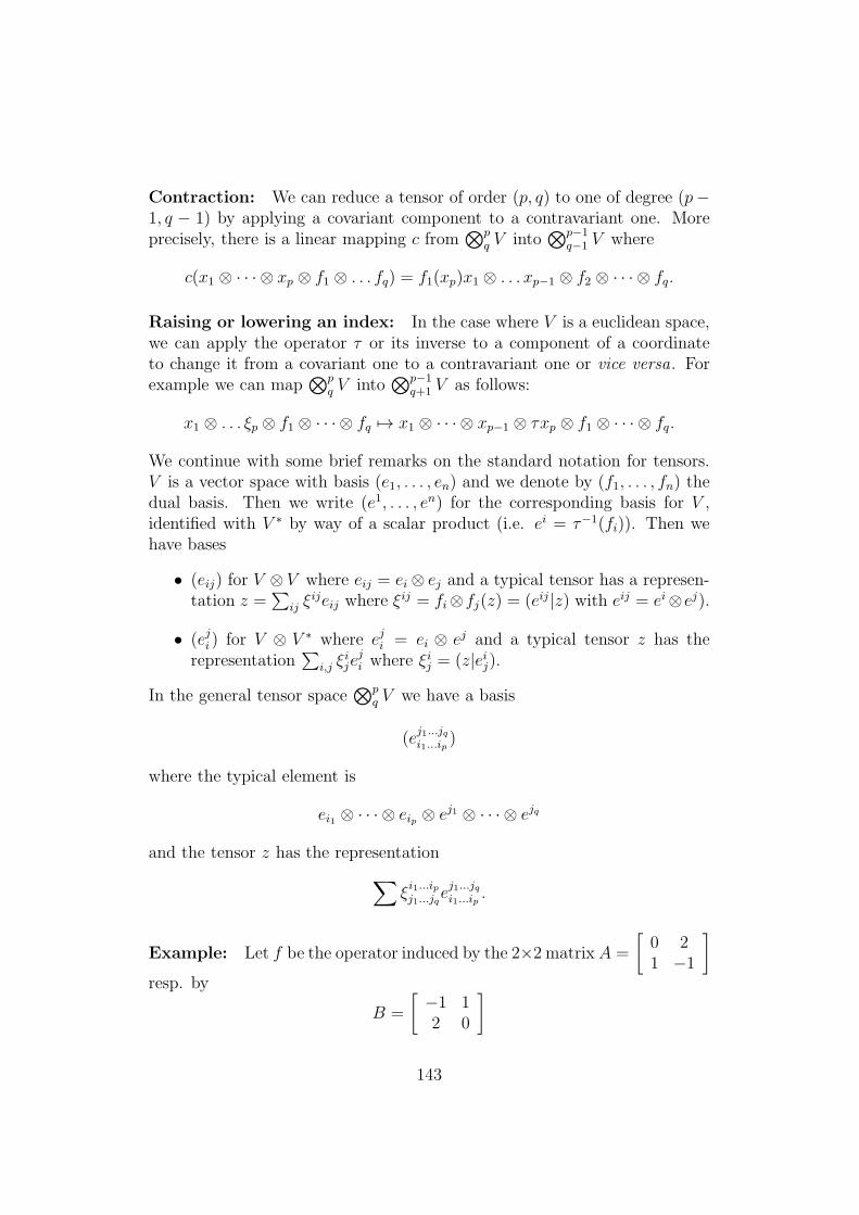
Contraction: We can reduce a tensor of order (p, q) to one of degree (p−1, q − 1) by applying a covariant component to a contravariant one. Moreprecisely, there is a linear mapping c from
⊗pq V into
⊗p−1q−1 V where
c(x1 ⊗ · · · ⊗ xp ⊗ f1 ⊗ . . . fq) = f1(xp)x1 ⊗ . . . xp−1 ⊗ f2 ⊗ · · · ⊗ fq.
Raising or lowering an index: In the case where V is a euclidean space,we can apply the operator τ or its inverse to a component of a coordinateto change it from a covariant one to a contravariant one or vice versa. Forexample we can map
⊗pq V into
⊗p−1q+1 V as follows:
x1 ⊗ . . . ξp ⊗ f1 ⊗ · · · ⊗ fq 7→ x1 ⊗ · · · ⊗ xp−1 ⊗ τxp ⊗ f1 ⊗ · · · ⊗ fq.
We continue with some brief remarks on the standard notation for tensors.V is a vector space with basis (e1, . . . , en) and we denote by (f1, . . . , fn) thedual basis. Then we write (e1, . . . , en) for the corresponding basis for V ,identified with V ∗ by way of a scalar product (i.e. ei = τ−1(fi)). Then wehave bases
• (eij) for V ⊗ V where eij = ei ⊗ ej and a typical tensor has a represen-tation z =
∑ij ξ
ijeij where ξij = fi⊗fj(z) = (eij |z) with eij = ei⊗ej).
• (eji ) for V ⊗ V ∗ where eji = ei ⊗ ej and a typical tensor z has therepresentation
∑i,j ξ
ije
ji where ξ
ij = (z|eij).
In the general tensor space⊗p
q V we have a basis
(ej1...jqi1...ip
)
where the typical element is
ei1 ⊗ · · · ⊗ eip ⊗ ej1 ⊗ · · · ⊗ ejq
and the tensor z has the representation
∑ξi1...ipj1...jq
ej1...jqi1...ip
.
Example: Let f be the operator induced by the 2×2 matrix A =
[0 21 −1
]
resp. by
B =
[−1 12 0
]
143

. We calculate the matrix of f ⊗ g with respect to the basis (y1, y2, y3, y4)where
y1 = e1 ⊗ e1 y2 = e1 ⊗ e2 y3 = e2 ⊗ e1 y4 = e4 ⊗ e4.
Then
f(y1) = −y3 + 2y4
f(y2) = y3
f(y3) = −2y1 + 4y2 + y3 − 2y4
f(y4) = 2y1 − y3.
Hence the required matrix is
0 0 −2 20 0 4 0−1 1 1 −12 0 −2 0
.
We can write this in the suggestive form
0
[−1 12 0
]2
[−1 12 0
]
1
[−1 12 0
]−1
[−1 12 0
]
from which the following general pattern should be clear.
Proposition 50 If A is the matrix of the linear mapping f and B that ofg, then the matrix of f ⊗ f is
a11B a12B . . . a1nB...
...an1B a2nB . . . annB
.
(This matrix is called the Kronecker product of A and B—written A⊗B).
Note that the basis used to define the matrix of the tensor product is that onewhich is obtained by considering the array (xi ⊗ yn) of tensor products andnumbering it by reading along the successive rows n the customary manner.
Using these matrix representation one can check the following results:
• if f and g are injective, then so is f ⊗ g;
144
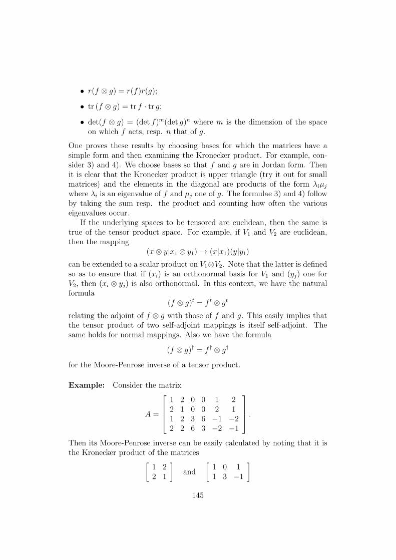
• r(f ⊗ g) = r(f)r(g);
• tr (f ⊗ g) = tr f · tr g;
• det(f ⊗ g) = (det f)m(det g)n where m is the dimension of the spaceon which f acts, resp. n that of g.
One proves these results by choosing bases for which the matrices have asimple form and then examining the Kronecker product. For example, con-sider 3) and 4). We choose bases so that f and g are in Jordan form. Thenit is clear that the Kronecker product is upper triangle (try it out for smallmatrices) and the elements in the diagonal are products of the form λiµj
where λi is an eigenvalue of f and µj one of g. The formulae 3) and 4) followby taking the sum resp. the product and counting how often the variouseigenvalues occur.
If the underlying spaces to be tensored are euclidean, then the same istrue of the tensor product space. For example, if V1 and V2 are euclidean,then the mapping
(x⊗ y|x1 ⊗ y1) 7→ (x|x1)(y|y1)can be extended to a scalar product on V1⊗V2. Note that the latter is definedso as to ensure that if (xi) is an orthonormal basis for V1 and (yj) one forV2, then (xi ⊗ yj) is also orthonormal. In this context, we have the naturalformula
(f ⊗ g)t = f t ⊗ gt
relating the adjoint of f ⊗ g with those of f and g. This easily implies thatthe tensor product of two self-adjoint mappings is itself self-adjoint. Thesame holds for normal mappings. Also we have the formula
(f ⊗ g)† = f † ⊗ g†
for the Moore-Penrose inverse of a tensor product.
Example: Consider the matrix
A =
1 2 0 0 1 22 1 0 0 2 11 2 3 6 −1 −22 2 6 3 −2 −1
.
Then its Moore-Penrose inverse can be easily calculated by noting that it isthe Kronecker product of the matrices
[1 22 1
]and
[1 0 11 3 −1
]
145
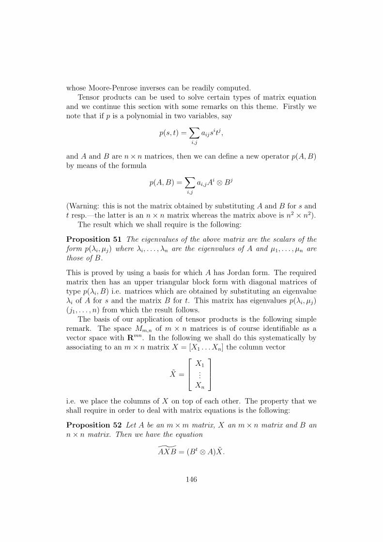
whose Moore-Penrose inverses can be readily computed.Tensor products can be used to solve certain types of matrix equation
and we continue this section with some remarks on this theme. Firstly wenote that if p is a polynomial in two variables, say
p(s, t) =∑
i,j
aijsitj,
and A and B are n× n matrices, then we can define a new operator p(A,B)by means of the formula
p(A,B) =∑
i,j
ai,jAi ⊗ Bj
(Warning: this is not the matrix obtained by substituting A and B for s andt resp.—the latter is an n× n matrix whereas the matrix above is n2 × n2).
The result which we shall require is the following:
Proposition 51 The eigenvalues of the above matrix are the scalars of theform p(λi, µj) where λi, . . . , λn are the eigenvalues of A and µ1, . . . , µn arethose of B.
This is proved by using a basis for which A has Jordan form. The requiredmatrix then has an upper triangular block form with diagonal matrices oftype p(λi, B) i.e. matrices which are obtained by substituting an eigenvalueλi of A for s and the matrix B for t. This matrix has eigenvalues p(λi, µj)(j1, . . . , n) from which the result follows.
The basis of our application of tensor products is the following simpleremark. The space Mm,n of m × n matrices is of course identifiable as avector space with Rmn. In the following we shall do this systematically byassociating to an m× n matrix X = [X1 . . .Xn] the column vector
X =
X1...Xn
i.e. we place the columns of X on top of each other. The property that weshall require in order to deal with matrix equations is the following:
Proposition 52 Let A be an m×m matrix, X an m× n matrix and B ann× n matrix. Then we have the equation
AXB = (Bt ⊗A)X.
146
Proof. If X = [X1 . . .Xn] then the j-th column of AXB is∑n
k=1(bjkA)Xk
and this is[b1jA b2jA . . . bnjA]X
which implies the result.The following special cases will be useful below.
AX = (In ⊗A)X ;
XB = (Bt ⊗ Im)X ;
˜AX +XB = ((In ⊗A) + (Bt ⊗ Im)X.
The above results can be used to tackle equations of the form
A1XB1 + · · ·+ ArXBr = C.
Here the A’s are the given m×m matrices, the B’s are n×n and V is m×n.X is the unknown. Using the above apparatus, we can rewrite the equationin the form GX = C where C =
∑rj=1B
tj ⊗ Aj.
Rather than consider the most general case, we shall confine our attentionto one special one which often occurs in applications, namely the equation
AX +XB = C.
In this case, the matrix G is
In ⊗ A+Bt ⊗ Im.
This is just p(A,Bt) where p(s, t) = s+t. Hence by our preparatory remarks,the eigenvalues of G are the scalars of the form λi +µj where the λ’s are theeigenvalues of A and the µj are those of B.
Hence we have proved the following result:
Proposition 53 The equation AX + XB = C has a solution for any C ifand only if λi + µj 6= 0 for each pair λi and µj of eigenvalues of A and Brespectively.
For the above condition means that 0 is not an eigenvalue of G i.e. thismatrix is invertible.
We can also get information for the case where the above general equationis not always solvable. Consider, for example, the equation
AXB = C
147

where we are not assuming that A and B are invertible. Suppose that S andT are generalised inverses for A and B respectively. Then it is clear thatS ⊗ T is one for A⊗ B. If we rewrite the equation AXB = C in the form
(At ⊗ B)X = C
then it follows form the general theory of such inverses that it has a solutionif and only if we have the equality
ASCTB = C.
The general solution is then
X = SCT + Y − SAY BT
whereby Y is arbitrary.In general, one would choose the Moore-Penrose inverses A† and B† for
S and T . This gives the solution
X = A†CB†
which is best possible in the usual sense.
Exercises: 1) Let x1, . . . , xn be elements of V . Show that
x1 ⊗ · · · ⊗ xn = 0
if and only if at least one xi vanishes. If x, y, x′, y′ are non-vanishing elements
of V show that x⊗ y = x′ ⊗ y′ if and only if there is a λ ∈ R so that x = λx′
and y = 1λy′.
2) Let V1 and V2 be vector spaces and denote by φ the natural bilinearmapping (x, y) 7→ x⊗y from V1×V2 into V1⊗V2. Show that for every bilinearmapping T : V1×V2 →W , there is a unique linear mapping f : V1⊗V2 → Wso that T = f ◦ φ.
Show that this property characterises the tensor product i.e. if U is avector space and ψ is a bilinear mapping from V1 × V2 into U so that thenatural analogue of the above property holds, then there is an isomorphismg from U onto V1 ⊗ V2 so that g ◦ ψ = φ.3) Let (xi) resp. (x′i) be bases for the vector space V and suppose thatA = [aij ] is the corresponding transfer matrix. Show that if a p-tensor z hasthe coordinate representation
z =∑
1≤i1,...,ip≤n
ti1,...,ipfi1 ⊗ · · · ⊗ fip
148

with respect to the first basis and
z =∑
1≤i1,...,ip≤n
t′i1,...,ipf′i1 ⊗ · · · ⊗ f ′
ip
with respect to the second, then
t′i1,...,ip =∑
1≤j1,...,jp≤n
ai1j1 . . . aipjptj1...jp.
4) Show that the tensor product
Pol (m)⊗ Pol (n)
is naturally isomorphic to the vector space of polynomials in two variable, ofdegree at most m in the first and at most n in the second.5) What is the trace resp. the determinant of the linear mapping
f 7→ φ ◦ f ◦ ψ
on L(V ) where φ and ψ are fixed members of L(V ).6) Consider the linear mapping
Φ : f 7→ f t
on L(V ) where V is Hermitian. Calculate the matrix of f with respect to theusual basis for L(V ) derived from an orthonormal basis for V . Is Φ normalresp. unitary with respect to the scalar product
(f |g) = tr (gtf).
Calculate the characteristic polynomial resp. the eigenvalues of Φ.7) Let p and q be polynomials and A and B be matrices with p and q ascharacteristic polynomials (for example, the companion matrices of p and q).Show that the number ∆ = det(A⊗ I − I ⊗B) is a resolvent of p and q i.e.has the property that it vanishes if and only if p and q have a common zero.8) Consider the mapping
X 7→ AXAt
on the vector space of the n×n symmetric matrices, where A is a given n×nmatrix. Show that the determinant of this mapping is (detA)n+1.
149