linear algebra - mml-book.github.io · linear algebra 744 745 when formalizing ... therefore,...

2

Linear Algebra

630

When formalizing intuitive concepts, one common approach is to con-631

struct a set of objects (symbols) and a set of rules to manipulate these632

objects. This is known as an algebra.633

Linear algebra is the study of vectors. The vectors many of us know634

from school are called “geometric vectors”, which are usually denoted by635

having a small arrow above the letter, e.g., −→x and −→y . In this book, we636

discuss more general concepts of vectors and use a bold letter to represent637

them, e.g., x and y.638

In general, vectors are special objects that can be added together and639

multiplied by scalars to produce another object of the same kind. Any640

object that satisfies these two properties can be considered a vector. Here641

are some examples of such vector objects:642

1. Geometric vectors. This example of a vector may be familiar from school.643

Geometric vectors are directed segments, which can be drawn, see644

Figure 2.1(a). Two geometric vectors x,y can be added, such that645

x + y = z is another geometric vector. Furthermore, multiplication646

by a scalar λx, λ ∈ R is also a geometric vector. In fact, it is the orig-647

inal vector scaled by λ. Therefore, geometric vectors are instances of648

the vector concepts introduced above.649

2. Polynomials are also vectors, see Figure 2.1(b): Two polynomials can650

be added together, which results in another polynomial; and they can651

be multiplied by a scalar λ ∈ R, and the result is a polynomial as652

well. Therefore, polynomials are (rather unusual) instances of vectors.653

Note that polynomials are very different from geometric vectors. While654

geometric vectors are concrete “drawings”, polynomials are abstract655

concepts. However, they are both vectors in the sense described above.656

Figure 2.1Different types ofvectors. Vectors canbe surprisingobjects, includinggeometric vectors,shown in (a), andpolynomials, shownin (b).

~x

~y

(a) Geometric vectors.

4 2 0 2 4 6 8

x

10

5

0

5

10

15

20

f(x)

(b) Polynomials.

13Draft chapter (May 28, 2018) from “Mathematics for Machine Learning” c©2018 by Marc PeterDeisenroth, A Aldo Faisal, and Cheng Soon Ong. To be published by Cambridge University Press.Report errata and feedback to http://mml-book.com. Please do not post or distribute this file,please link to http://mml-book.com.

http://mml-book.com

http://mml-book.com

14 Linear Algebra

3. Audio signals are vectors. Audio signals are represented as a series of657

numbers. We can add audio signals together, and their sum is a new658

audio signal. If we scale an audio signal, we also obtain an audio signal.659

Therefore, audio signals are a type of vector, too.660

4. Elements of Rn are vectors. In other words, we can consider each el-ement of Rn (the tuple of n real numbers) to be a vector. Rn is moreabstract than polynomials, and it is the concept we focus on in thisbook. For example,

a =

123

∈ R3 (2.1)

is an example of a triplet of numbers. Adding two vectors a, b ∈ Rn661

component-wise results in another vector: a+ b = c ∈ Rn. Moreover,662

multiplying a ∈ Rn by λ ∈ R results in a scaled vector λa ∈ Rn.663

Linear algebra focuses on the similarities between these vector concepts.664

We can add them together and multiply them by scalars. We will largely665

focus on vectors in Rn since most algorithms in linear algebra are for-666

mulated in Rn. Recall that in machine learning, we often consider data667

to be represented as vectors in Rn. In this book, we will focus on finite-668

dimensional vector spaces, in which case there is a 1:1 correspondence669

between any kind of (finite-dimensional) vector and Rn. By studying Rn,670

we implicitly study all other vectors such as geometric vectors and poly-671

nomials. Although Rn is rather abstract, it is most useful.672

One major idea in mathematics is the idea of “closure”. This is the ques-673

tion: What is the set of all things that can result from my proposed oper-674

ations? In the case of vectors: What is the set of vectors that can result by675

starting with a small set of vectors, and adding them to each other and676

scaling them? This results in a vector space (Section 2.4). The concept of677

a vector space and its properties underlie much of machine learning.678

A closely related concept is a matrix, which can be thought of as amatrix 679

collection of vectors. As can be expected, when talking about properties680

of a collection of vectors, we can use matrices as a representation. The681

concepts introduced in this chapter are shown in Figure 2.2682

This chapter is largely based on the lecture notes and books by Drumm683

and Weil (2001); Strang (2003); Hogben (2013); Liesen and Mehrmann684

(2015) as well as Pavel Grinfeld’s Linear Algebra series1. Another excellent685

source is Gilbert Strang’s Linear Algebra course at MIT2.686

Linear algebra plays an important role in machine learning and gen-687

eral mathematics. In Chapter 5, we will discuss vector calculus, where688

a principled knowledge of matrix operations is essential. In Chapter 11,689

1http://tinyurl.com/nahclwm2http://tinyurl.com/29p5q8j

Draft (2018-05-28) from Mathematics for Machine Learning. Errata and feedback to http://mml-book.com.

http://mml-book.com

2.1 Systems of Linear Equations 15

Figure 2.2 A mindmap of the conceptsintroduced in thischapter, along withwhen they are usedin other parts of thebook.

Vector

Vector spaceMatrixChapter 5Vector calculus

Group

Linear systemof equations

Matrixinverse

Gaussianelimination

Linear/affinemapping

Linearindependence

Basis

Chapter 11Dimensionality

reduction

Chapter 10Classification

Chapter 3Analytic geometry

setof

(+, ·), closure

used in requires

transfo

rms

represented asrepres

ented

as

solves

solved by

property of

min

imal

set

usedin

usedin

usedin

used

in

we will use projections (to be introduced in Section 3.6) for dimensional-690

ity reduction with Principal Component Analysis (PCA). In Chapter 9, we691

will discuss linear regression where linear algebra plays a central role for692

solving least-squares problems.693

2.1 Systems of Linear Equations694

Systems of linear equations play a central part of linear algebra. Many695

problems can be formulated as systems of linear equations, and linear696

algebra gives us the tools for solving them.697

ExampleA company produces productsN1, . . . , Nn for which resourcesR1, . . . , Rmare required. To produce a unit of product Nj , aij units of resource Ri areneeded, where i = 1, . . . ,m and j = 1, . . . , n.

The objective is to find an optimal production plan, i.e., a plan of howmany units xj of product Nj should be produced if a total of bi units ofresource Ri are available and (ideally) no resources are left over.

If we produce x1, . . . , xn units of the corresponding products, we needa total of

ai1x1 + · · ·+ ainxn (2.2)

many units of resource Ri. The optimal production plan (x1, . . . , xn) ∈Rn, therefore, has to satisfy the following system of equations:

a11x1 + · · ·+ a1nxn...

am1x1 + · · ·+ amnxn

=

b1

...bm

, (2.3)

c©2018 Marc Peter Deisenroth, A. Aldo Faisal, Cheng Soon Ong. To be published by Cambridge University Press.

16 Linear Algebra

where aij ∈ R and bi ∈ R.

Equation (2.3) is the general form of a system of linear equations, andsystem of linearequations

698

x1, . . . , xn are the unknowns of this system of linear equations. Every n-unknowns

699

tuple (x1, . . . , xn) ∈ Rn that satisfies (2.3) is a solution of the linear equa-solution

700

tion system.701

ExampleThe system of linear equations

x1 + x2 + x3 = 3 (1)x1 − x2 + 2x3 = 2 (2)2x1 + 3x3 = 1 (3)

(2.4)

has no solution: Adding the first two equations yields (1) + (2) = 2x1 +3x3 = 5, which contradicts the third equation (3).

Let us have a look at the system of linear equations

x1 + x2 + x3 = 3 (1)x1 − x2 + 2x3 = 2 (2)

x2 + x3 = 2 (3). (2.5)

From the first and third equation it follows that x1 = 1. From (1)+(2) weget 2+3x3 = 5, i.e., x3 = 1. From (3), we then get that x2 = 1. Therefore,(1, 1, 1) is the only possible and unique solution (verify that (1, 1, 1) is asolution by plugging in).

As a third example, we consider

x1 + x2 + x3 = 3 (1)x1 − x2 + 2x3 = 2 (2)2x1 + 3x3 = 5 (3)

. (2.6)

Since (1)+(2)=(3), we can omit the third equation (redundancy). From(1) and (2), we get 2x1 = 5−3x3 and 2x2 = 1+x3. We define x3 = a ∈ Ras a free variable, such that any triplet(

5

2− 3

2a,

1

2+

1

2a, a

), a ∈ R (2.7)

is a solution to the system of linear equations, i.e., we obtain a solutionset that contains infinitely many solutions.

In general, for a real-valued system of linear equations we obtain either702

no, exactly one or infinitely many solutions.703

Remark (Geometric Interpretation of Systems of Linear Equations). In a704

system of linear equations with two variables x1, x2, each linear equation705

determines a line on the x1x2-plane. Since a solution to a system of lin-706


http://mml-book.com

2.2 Matrices 17

Figure 2.3 Thesolution space of asystem of two linearequations with twovariables can begeometricallyinterpreted as theintersection of twolines. Every linearequation representsa line.

2x1 − 4x2 = 1

4x1 + 4x2 = 5

x1

x2

ear equations must satisfy all equations simultaneously, the solution set707

is the intersection of these line. This intersection can be a line (if the lin-708

ear equations describe the same line), a point, or empty (when the lines709

are parallel). An illustration is given in Figure 2.3. Similarly, for three710

variables, each linear equation determines a plane in three-dimensional711

space, and the solution set is the intersection of these planes, which can712

be a plane, a line, a point or empty (when the planes are parallel). ♦713

For a systematic approach to solving systems of linear equations, we willintroduce a useful compact notation. We will write the system from (2.3)in the following form:

x1

a11

...am1

+ x2

a12

...am2

+ · · ·+ xn

a1n

...amn

=

b1

...bm

(2.8)

⇐⇒

a11 · · · a1n

......

am1 · · · amn

x1

...xn

=

b1

...bm

. (2.9)

In the following, we will have a close look at these matrices and define714

computation rules.715

2.2 Matrices716

Matrices play a central role in linear algebra. They can be used to com-717

pactly represent linear equation systems, but they also represent linear718

functions (linear mappings) as we will see later. Before we discuss some719

of these interesting topics, let us first define what a matrix is and what720

kind of operations we can do with matrices.721

Definition 2.1 (Matrix). With m,n ∈ N a real-valued (m,n) matrix A is matrix

anm·n-tuple of elements aij , i = 1, . . . ,m, j = 1, . . . , n, which is ordered


18 Linear Algebra

according to a rectangular scheme consisting of m rows and n columns:

A =

a11 a12 · · · a1n

a21 a22 · · · a2n

......

...am1 am2 · · · amn

, aij ∈ R . (2.10)

(1, n)-matrices are called rows, (m, 1)-matrices are called columns. Theserowscolumns

722

special matrices are also called row/column vectors.row/column vectors

723

Rm×n is the set of all real-valued (m,n)-matrices. A ∈ Rm×n can be724

equivalently represented as a ∈ Rmn by stacking all n columns of the725

matrix into a long vector.726

2.2.1 Matrix Multiplication727

For A ∈ Rm×n,B ∈ Rn×k the elements cij of the product C = AB ∈Note the size of thematrices! Rm×k are defined asC =np.einsum(’il,lj’, A, B) cij =

n∑l=1

ailblj, i = 1, . . . ,m, j = 1, . . . , k. (2.11)

This means, to compute element cij we multiply the elements of the ithThere are n columnsin A and n rows inB, such that we cancompute ailblj forl = 1, . . . , n.

728

row ofA with the jth column ofB and sum them up. Later in Section ??,729

we will call this the dot product of the corresponding row and column.730

Remark. Matrices can only be multiplied if their “neighboring” dimensionsmatch. For instance, an n × k-matrix A can be multiplied with a k ×m-matrix B, but only from the left side:

A︸︷︷︸n×k

B︸︷︷︸k×m

= C︸︷︷︸n×m

(2.12)

The productBA is not defined ifm 6= n since the neighboring dimensions731

do not match. ♦732This kind ofelement-wisemultiplicationappears often incomputer sciencewhere we multiply(multi-dimensional)arrays with eachother.

Remark. Note that matrix multiplication is not defined as an element-wise733

operation on matrix elements, i.e., cij 6= aijbij (even if the size of A,B734

was chosen appropriately). ♦735

Example

For A =

[1 2 33 2 1

]∈ R2×3, B =

0 21 −10 1

∈ R3×2, we obtain

AB =

[1 2 33 2 1

]0 21 −10 1

=

[2 32 5

]∈ R2×2, (2.13)


http://mml-book.com

2.2 Matrices 19

BA =

0 21 −10 1

[1 2 33 2 1

]=

6 4 2−2 0 23 2 1

∈ R3×3 . (2.14)

Figure 2.4 Even ifboth matrixmultiplications ABand BA aredefined, thedimensions of theresults can bedifferent.

From this example, we can already see that matrix multiplication is not736

commutative, i.e., AB 6= BA, see also Figure 2.4 for an illustration.737

Definition 2.2 (Identity Matrix). In Rn×n, we define the identity matrix

identity matrix

as

In =

1 0 · · · 0 · · · 00 1 · · · 0 · · · 0...

.... . .

.... . .

...0 0 · · · 1 · · · 0...

.... . .

.... . .

...0 0 · · · 0 · · · 1

∈ Rn×n (2.15)

as the n × n-matrix containing 1 on the diagonal and 0 everywhere else.738

With this, A · In = A = In ·A for all A ∈ Rn×n.739

Now that we have defined matrix multiplication, matrix addition and740

the identity matrix, let us have a look at some properties of matrices,741

where we will omit the “·” for matrix multiplication:742

• Associativity:

∀A ∈ Rm×n,B ∈ Rn×p,C ∈ Rp×q : (AB)C = A(BC) (2.16)

• Distributivity:

∀A1,A2 ∈ Rm×n,B ∈ Rn×p :(A1 +A2)B = A1B +A2B (2.17)

A(B +C) = AB +AC (2.18)

• Neutral element:

∀A ∈ Rm×n : ImA = AIn = A (2.19)

Note that Im 6= In for m 6= n.743

2.2.2 Inverse and Transpose744

Definition 2.3 (Inverse). For a square matrix3 A ∈ Rn×n a matrix B ∈745

Rn×n with AB = In = BA the matrix B is called inverse and denoted inverse746

by A−1.747

Unfortunately, not every matrix A possesses an inverse A−1. If this748

inverse does exist, A is called regular/invertible/non-singular, otherwise regular

invertiblenon-singular

749

singular/non-invertible.

singular

non-invertible

750

3The number of columns equals the number of rows.


20 Linear Algebra

Example (Inverse Matrix)The matrices

A =

1 2 14 4 56 7 7

, B =

−7 −7 62 1 −14 5 −4

(2.20)

are inverse to each other since AB = I = BA.

Definition 2.4 (Transpose). For A ∈ Rm×n the matrix B ∈ Rn×m with751

bij = aji is called the transpose of A. We write B = A>.transpose 752

The main diagonal(sometimes called“principal diagonal”,“primary diagonal”,“leading diagonal”,or “major diagonal”)of a matrix A is thecollection of entriesAij where i = j.

For a square matrixA> is the matrix we obtain when we “mirror”A on753

its main diagonal. In general,A> can be obtained by writing the columns754

of A as the rows of A>.755

Let us have a look at some important properties of inverses and trans-756

poses:757

• AA−1 = I = A−1A758

• (AB)−1 = B−1A−1759

• (A>)> = A760

• (A+B)> = A> +B>761

• (AB)> = B>A>762

• If A is invertible, (A−1)> = (A>)−1763

• Note: (A+B)−1 6= A−1 +B−1. Example: in the scalar case 12+4

= 166=764

12

+ 14.765

A matrix A is symmetric if A = A>. Note that this can only hold forsymmetric

(n, n)-matrices, which we also call square matrices because they possessquare matrices

the same number of rows and columns. The sum of symmetric matrices issymmetric, but this does not hold for the product in general (although itis always defined). A counterexample is[

1 00 0

] [1 11 1

]=

[1 10 0

]. (2.21)

2.2.3 Multiplication by a Scalar766

Let us have a brief look at what happens to matrices when they are mul-767

tiplied by a scalar λ ∈ R. Let A ∈ Rm×n and λ ∈ R. Then λA = K,768

Kij = λ aij . Practically, λ scales each element ofA. For λ, ψ ∈ R it holds:769

• Distributivity:770

(λ+ ψ)C = λC + ψC, C ∈ Rm×n771

λ(B +C) = λB + λC, B,C ∈ Rm×n772


http://mml-book.com

2.3 Solving Systems of Linear Equations 21

• Associativity:773

(λψ)C = λ(ψC), C ∈ Rm×n774

λ(BC) = (λB)C = B(λC) = (BC)λ, B ∈ Rm×n,C ∈ Rn×k.775

Note that this allows us to move scalar values around.776

• (λC)> = C>λ> = C>λ = λC> since λ = λ> for all λ ∈ R.777

2.2.4 Compact Representations of Systems of Linear Equations778

If we consider the system of linear equations

2x1 + 3x2 + 5x3 = 1

4x1 − 2x2 − 7x3 = 8

9x1 + 5x2 − 3x3 = 2

and use the rules for matrix multiplication, we can write this equationsystem in a more compact form as2 3 5

4 −2 −79 5 −3

x1

x2

x3

=

182

. (2.22)

Note that x1 scales the first column, x2 the second one, and x3 the third779

one.780

Generally, system of linear equations can be compactly represented in781

their matrix form as Ax = b, see (2.3), and the product Ax is a (linear)782

combination of the columns of A. We will discuss linear combinations in783

more detail in Section 2.5.784

2.3 Solving Systems of Linear Equations785

In (2.3), we introduced the general form of an equation system, i.e.,

a11x1 + · · ·+ a1nxn...

am1x1 + · · ·+ amnxn

= b1

...= bm

, (2.23)

where aij ∈ R and bi ∈ R are known constants and xj are unknowns,786

i = 1, . . . ,m, j = 1, . . . , n. Thus far, we saw that matrices can be used as787

a compact way of formulating systems of linear equations so that we can788

write Ax = b, see (2.9). Moreover, we defined basic matrix operations,789

such as addition and multiplication of matrices. In the following, we will790

focus on solving systems of linear equations.791

2.3.1 Particular and General Solution792

Before discussing how to solve systems of linear equations systematically,let us have a look at an example. Consider the following system of equa-


22 Linear Algebra

tions:

[1 0 8 −40 1 2 12

]x1

x2

x3

x4

=

[428

]. (2.24)

This equation system is in a particularly easy form, where the first twocolumns consist of a 1 and a 0. Remember that we want to find scalarsLater, we will say

that this matrix is inreduced rowechelon form.

x1, . . . , x4, such that∑4

i=1 xici = b, where we define ci to be the ithcolumn of the matrix and b the right-hand-side of (2.24). A solution tothe problem in (2.24) can be found immediately by taking 42 times thefirst column and 8 times the second column so that

b =

[428

]= 42

[10

]+ 8

[01

]. (2.25)

Therefore, a solution vector is [42, 8, 0, 0]>. This solution is called a particularparticular solution

solution or special solution. However, this is not the only solution of thisspecial solution

system of linear equations. To capture all the other solutions, we need tobe creative of generating 0 in a non-trivial way using the columns of thematrix: Adding 0 to our special solution does not change the special so-lution. To do so, we express the third column using the first two columns(which are of this very simple form)[

82

]= 8

[10

]+ 2

[01

], (2.26)

such that 0 = 8c1 + 2c2 − 1c3 + 0c4, and (x1, x2, x3, x4) = (8, 2,−1, 0).In fact, any scaling of this solution by λ1 ∈ R produces the 0 vector:

[1 0 8 −40 1 2 12

]λ1

82−10

= λ1(8c1 + 2c2 − c3) = 0 . (2.27)

Following the same line of reasoning, we express the fourth column of thematrix in (2.24) using the first two columns and generate another set ofnon-trivial versions of 0 as

[1 0 8 −40 1 2 12

]λ2

−4120−1

= λ2(−4c1 + 12c2 − c4) = 0 (2.28)

for any λ2 ∈ R. Putting everything together, we obtain all solutions of theequation system in (2.24), which is called the general solution, as the setgeneral solution x ∈ R4 : x =

42800

+ λ1

82−10

+ λ2

−4120−1

, λ1, λ2 ∈ R

. (2.29)


http://mml-book.com


Remark. The general approach we followed consisted of the following793

three steps:794

1. Find a particular solution to Ax = b795

2. Find all solutions to Ax = 0796

3. Combine the solutions from 1. and 2. to the general solution.797

Neither the general nor the particular solution is unique. ♦798

The system of linear equations in the example above was easy to solve799

because the matrix in (2.24) has this particularly convenient form, which800

allowed us to find the particular and the general solution by inspection.801

However, general equation systems are not of this simple form. Fortu-802

nately, there exists a constructive algorithmic way of transforming any803

system of linear equations into this particularly simple form: Gaussian804

elimination. Key to Gaussian elimination are elementary transformations805

of systems of linear equations, which transform the equation system into a806

simple form. Then, we can apply the three steps to the simple form that we807

just discussed in the context of the example in (2.24), see Remark 2.3.1.808

2.3.2 Elementary Transformations809

Key to solving a system of linear equations are elementary transformations elementarytransformations

810

that keep the solution set the same, but that transform the equation system811

into a simpler form:812

• Exchange of two equations (or: rows in the matrix representing the813

equation system)814

• Multiplication of an equation (row) with a constant λ ∈ R\{0}815

• Addition an equation (row) to another equation (row)816

ExampleWe want to find the solutions of the following system of equations:

−2x1 + 4x2 − 2x3 − x4 + 4x5 = −34x1 − 8x2 + 3x3 − 3x4 + x5 = 2x1 − 2x2 + x3 − x4 + x5 = 0x1 − 2x2 − 3x4 + 4x5 = a

, a ∈ R .

(2.30)

We start by converting this system of equations into the compact matrixnotation Ax = b. We no longer mention the variables x explicitly andbuild the augmented matrix augmented matrix

−2 4 −2 −1 4 −34 −8 3 −3 1 21 −2 1 −1 1 01 −2 0 −3 4 a

Swap with R3

Swap with R1


24 Linear Algebra

where we used the vertical line to separate the left-hand-side from theThe augmentedmatrix

[A | b

]compactlyrepresents thesystem of linearequations Ax = b.

right-hand-side in (2.30). Swapping rows 1 and 3 leads to1 −2 1 −1 1 04 −8 3 −3 1 2−2 4 −2 −1 4 −3

1 −2 0 −3 4 a

−4R1

+2R1

−R1

When we now apply the indicated transformations (e.g., subtract Row 1 4times from Row 2), we obtain

1 −2 1 −1 1 00 0 −1 1 −3 20 0 0 −3 6 −30 0 −1 −2 3 a

−R2

1 −2 1 −1 1 00 0 −1 1 −3 20 0 0 −3 6 −30 0 0 −3 6 a−2

−R3

1 −2 1 −1 1 00 0 −1 1 −3 20 0 0 −3 6 −30 0 0 0 0 a+1

·(−1)·(− 1

3)

1 −2 1 −1 1 00 0 1 −1 3 −20 0 0 1 −2 10 0 0 0 0 a+1

This (augmented) matrix is in a convenient form, the row-echelon formrow-echelon form

(REF) (REF). Reverting this compact notation back into the explicit notation withthe variables we seek, we obtain

x1 − 2x2 + x3 − x4 + x5 = 0x3 − x4 + 3x5 = −2

x4 − 2x5 = 10 = a+ 1

. (2.31)

Only for a = −1, this equation system can be solved. A particular solutionparticular solution

is given by x1

x2

x3

x4

x5

=

20−110

(2.32)


http://mml-book.com


and the general solution, which captures the set of all possible solutions, general solution

is given asx ∈ R5 : x =

20−110

+ λ1

21000

+ λ2

20−121

, λ1, λ2 ∈ R .

(2.33)

Remark (Pivots and Staircase Structure). The leading coefficient of a row817

(the first nonzero number from the left) is called the pivot and is always pivot818

strictly to the right of the leading coefficient of the row above it. This en-819

sures that an equation system in row echelon form always has a “staircase”820

structure. ♦821

Definition 2.5 (Row-Echelon Form). A matrix is in row-echelon form (REF) row-echelon form822

if823

• All nonzero rows (rows with at least one nonzero element) are above824

any rows of all zeros (all zero rows, if any, belong at the bottom of the825

matrix), and826

• The leading coefficient (the first nonzero number from the left, also827

called the pivot) of a nonzero row is always strictly to the right of the828

leading coefficient of the row above it. In some literature, itis required that theleading coefficientof a matrix in REF is1.

829

Remark (Basic and Free Variables). The variables corresponding to the830

pivots in the row-echelon form are called basic variables, the other vari-

basic variables

831

ables are free variables. For example, in (2.31), x1, x3, x4 are basic vari-

free variables

832

ables, whereas x2, x5 are free variables. ♦833

Remark (Obtaining a Particular Solution). The row echelon form makes834

our lives easier when we need to determine a particular solution. To do835

this, we express the right-hand side of the equation system using the pivot836

columns, such that b =∑P

i=1 λipi, where pi, i = 1, . . . , P , are the pivot837

columns. The λi are determined easiest if we start with the most-right838

pivot column and work our way to the left.839

In the above example, we would try to find λ1, λ2, λ3 such that

λ1

1000

+ λ2

1100

+ λ3

−1−110

=

0−210

. (2.34)

From here, we find relatively directly that λ3 = 1, λ2 = −1, λ1 = 2. Whenwe put everything together, we must not forget the non-pivot columnsfor which we set the coefficients implicitly to 0. Therefore, we get the


26 Linear Algebra

particular solution

x =

20−110

. (2.35)

♦840

Remark (Reduced Row Echelon Form). An equation system is in reducedreduced rowechelon form

841

row echelon form (also: row-reduced echelon form or row canonical form) if842

• It is in row echelon form843

• Every pivot must be 1844

• The pivot is the only non-zero entry in its column.845

♦846

The reduced row echelon form will play an important role later in Sec-847

tion 2.3.3 because it allows us to determine the general solution of a sys-848

tem of linear equations in a straightforward way.849Gaussianelimination Remark (Gaussian Elimination). Gaussian elimination is an algorithm that850

performs elementary transformations to bring a system of linear equations851

into reduced row echelon form from which we can read out the general852

solution. ♦853

Example (Reduced Row Echelon Form)Verify that the following matrix is in reduced row echelon form (the pivotsare in bold):

A =

1 3 0 0 30 0 1 0 90 0 0 1 −4

(2.36)

The key idea for finding the solutions of Ax = 0 is to look at the non-pivot columns, which we will need to express as a (linear) combination ofthe pivot columns. The reduced row echelon form makes this relativelystraightforward, and we express the non-pivot columns in terms of sumsand multiples of the pivot columns that are on their left: The second col-umn is 3 times the first column (we can ignore the pivot columns on theright of the second column). Therefore, to obtain 0, we need to subtractthe second column from three times the first column. Now, we look at thefifth column, which is our second non-pivot column. The fifth column canbe expressed as 3 times the first pivot column, 9 times the second pivotcolumn, and −4 times the third pivot column. We need to keep track ofthe indices of the pivot columns and translate this into 3 times the first col-umn, 0 times the second column (which is a non-pivot column), 9 times


http://mml-book.com


the third pivot column (which is our second pivot column), and −4 timesthe fourth column (which is the third pivot column). Then we need tosubtract the fifth column to obtain 0—in the end, we are still solving ahomogeneous equation system.

To summarize, all solutions of Ax = 0,x ∈ R5 are given byx ∈ R5 : x = λ1

3−1000

+ λ2

309−4−1

, λ1, λ2 ∈ R

. (2.37)

2.3.3 The Minus-1 Trick854

In the following, we introduce a practical trick for reading out the solu-855

tions x of a homogeneous system of linear equations Ax = 0, where856

A ∈ Rk×n,x ∈ Rn.857

To start, we assume thatA is in reduced row echelon form without anyrows that just contain zeros, i.e.,

A =

0 · · · 0 1 ∗ · · · ∗ 0 ∗ · · · ∗ 0 ∗ · · · ∗...

... 0 0 · · · 0 1 ∗ · · · ∗ ......

......

......

...... 0 ∗ . . . ∗ 0

......

......

......

...... ∗ . . . ∗ 0

......

0 · · · 0 0 0 · · · 0 0 ∗ · · · ∗ 1 ∗ · · · ∗

,

(2.38)

where ∗ can be an arbitrary real number. Note that the columns j1, . . . , jkwith the pivots (marked in bold) are the standard unit vectors e1, . . . , ek ∈Rk. We now extend this matrix to an n×n-matrix A by adding n−k rowsof the form [

0 · · · 0 −1 0 · · · 0]

(2.39)

so that the diagonal of the augmented matrix A contains either 1 or −1.858

Then, the columns of A, which contain the −1 as pivots are solutions859

of the homogeneous equation system Ax = 0. To be more precise, these860

columns form a basis (Section 4.3) of the solution space ofAx = 0, which861

we will later call the kernel or null space (see Section 2.7.3). kernelnull space

862

Example (Minus-1 Trick)Let us revisit the matrix in (2.36), which is already in reduced row echelon


28 Linear Algebra

form:

A =

1 3 0 0 30 0 1 0 90 0 0 1 −4

. (2.40)

We now augment this matrix to a 5 × 5 matrix by adding rows of theform (2.39) at the places where the pivots on the diagonal are missingand obtain

A =

1 3 0 0 30 −1 0 0 00 0 1 0 90 0 0 1 −40 0 0 0 −1

(2.41)

From this form, we can immediately read out the solutions of Ax = 0 bytaking the columns of A, which contain −1 on the diagonal:x ∈ R

5 : x = λ1

3−1000

+ λ2

309−4−1

, λ1, λ2 ∈ R

, (2.42)

which is identical to the solution in (2.37) that we obtained by “insight”.

Calculating the Inverse863

To compute the inverse A−1 of A ∈ Rn×n, we need to find a matrix Xthat satisfies AX = In. Then, X = A−1. We can write this down asa set of simultaneous linear equations AX = In, where we solve forX = [x1| · · · |xn]. We use the augmented matrix notation for a compactrepresentation of this set of systems of linear equations and obtain[

A|In] · · ·

[In|A−1

]. (2.43)

This means that if we bring the augmented equation system into reduced864

row echelon form, we can read out the inverse on the right-hand side of865

the equation system. Hence, determining the inverse of a matrix is equiv-866

alent to solving systems of linear equations.867

Example (Calculating an Inverse Matrix by Gaussian Elimination)To determine the inverse of

A =

1 0 2 01 1 0 01 2 0 11 1 1 1

(2.44)


http://mml-book.com


we write down the augmented matrix1 0 2 0 1 0 0 01 1 0 0 0 1 0 01 2 0 1 0 0 1 01 1 1 1 0 0 0 1

and use Gaussian elimination to bring it into reduced row echelon form

1 0 0 0 −1 2 −2 20 1 0 0 1 −1 2 −20 0 1 0 1 −1 1 −10 0 0 1 −1 0 −1 2

,such that the desired inverse is given as its right-hand side:

A−1 =

−1 2 −2 21 −1 2 −21 −1 1 −1−1 0 −1 2

. (2.45)

2.3.4 Algorithms for Solving a System of Linear Equations868

In the following, we briefly discuss approaches to solving a system of lin-869

ear equations of the form Ax = b.870

In special cases, we may be able to determine the inverse A−1, suchthat the solution of Ax = b is given as x = A−1b. However, this is onlypossible ifA is a square matrix and invertible, which is often not the case.Otherwise, under mild assumptions we can use the transformation

Ax = b ⇐⇒ A>Ax = A>b ⇐⇒ x = (A>A)−1A>b (2.46)

and use the Moore-Penrose pseudo-inverse (A>A)−1A> to determine the871

solution (2.46) that solves Ax = b, which also corresponds to the mini-872

mum norm least-squares solution. A disadvantage of this approach is that873

it requires many computations for the matrix-matrix product and comput-874

ing the inverse of A>A. Moreover, for reasons of numerical precision it875

is generally not recommended to compute the inverse or pseudo-inverse.876

In the following, we therefore briefly discuss alternative approaches to877

solving systems of linear equations.878

Gaussian elimination plays an important role when computing determi-879

nants, checking whether a set of vectors is linearly independent, comput-880

ing the inverse of a matrix, computing the rank of a matrix and a basis of a881

vector space. We will discuss all these topics later on. Gaussian elimination882

is an intuitive and constructive way to solve a system of linear equations883

with thousands of variables. However, for systems with millions of vari-884


30 Linear Algebra

ables, it is impractical as the required number of arithmetic operations885

scales cubically in the number of simultaneous equations.886

In practice, systems of many linear equations are solved indirectly, by887

either stationary iterative methods, such as the Richardson method, the888

Jacobi method, the Gauß-Seidel method, or the successive over-relaxation889

method, or Krylov subspace methods, such as conjugate gradients, gener-890

alized minimal residual, or biconjugate gradients.891

Let x∗ be a solution ofAx = b. The key idea of these iterative methodsis to set up an iteration of the form

x(k+1) = Ax(k) (2.47)

that reduces the residual error ‖x(k+1)−x∗‖ in every iteration and finally892

converges to x∗. We will introduce norms ‖ · ‖, which allow us to compute893

similarities between vectors, in Section 3.1.894

2.4 Vector Spaces895

Thus far, we have looked at linear equation systems and how to solve896

them. We saw that linear equation systems can be compactly represented897

using matrix-vector notations. In the following, we will have a closer look898

at vector spaces, i.e., the space in which vectors live.899

In the beginning of this chapter, we informally characterized vectors as900

objects that can be added together and multiplied by a scalar, and they901

remain objects of the same type (see page 13). Now, we are ready to902

formalize this, and we will start by introducing the concept of a group,903

which is a set of elements and an operation defined on these elements904

that keeps some structure of the set intact.905

2.4.1 Groups906

Groups play an important role in computer science. Besides providing a907

fundamental framework for operations on sets, they are heavily used in908

cryptography, coding theory and graphics.909

Definition 2.6 (Group). Consider a set G and an operation⊗ : G×G → G910

defined on G.911

Then G := (G,⊗) is called a group if the following hold:group 912

Closure1. Closure of G under ⊗: ∀x, y ∈ G : x⊗ y ∈ G913Associativity:2. Associativity: ∀x, y, z ∈ G : (x⊗ y)⊗ z = x⊗ (y ⊗ z)914Neutral element:3. Neutral element: ∃e ∈ G ∀x ∈ G : x⊗ e = x and e⊗ x = x915Inverse element:4. Inverse element: ∀x ∈ G ∃y ∈ G : x ⊗ y = e and y ⊗ x = e. We often916

write x−1 to denote the inverse element of x.917

If additionally ∀x, y ∈ G : x ⊗ y = y ⊗ x then G = (G,⊗) is an AbelianAbelian group 918

group (commutative).919


http://mml-book.com

2.4 Vector Spaces 31

For example, ⊗ could be +, · defined on R,N,Z or ∪,∩, \ defined on920

P(B), the power set of B.921

Remark. The inverse element is defined with respect to the operation ⊗922

and does not necessarily mean 1x. ♦923

Example (Groups)Let us have a look at some examples of sets with associated operationsand see whether they are groups.

• (Z,+) is a group.• (N0,+)4 is not a group: Although (N0,+) possesses a neutral element

(0), the inverse elements are missing.• (Z, ·) is not a group: Although (Z, ·) contains a neutral element (1), the

inverse elements for any z ∈ Z, z 6= ±1, are missing.• (R, ·) is not a group since 0 does not possess an inverse element.• (R\{0}) is Abelian.• (Rn,+), (Zn,+), n ∈ N are Abelian if + is defined componentwise, i.e.,

(x1, · · · , xn) + (y1, · · · , yn) = (x1 + y1, · · · , xn + yn). (2.48)

Then, (x1, · · · , xn)−1 := (−x1, · · · ,−xn) is the inverse element ande = (0, · · · , 0) is the neutral element.• (Rm×n,+), the set of m × n-matrices is Abelian (with componentwise

addition as defined in (2.48)). If A ∈ Rm×n thenIn is only a rightneutral element,such thatAIn = A. Thecorrespondingleft-neutral elementwould be Im sinceImA = A.

• Let us have a closer look at (Rn×n, ·), i.e., the set of n×n-matrices withmatrix multiplication as defined in (2.11).

– Closure and associativity follow directly from the definition of matrixmultiplication.

– Neutral element: The identity matrix In is the neutral element withrespect to matrix multiplication “·” in (Rn×n, ·).

– Inverse element: If the inverse exists thenA−1 is the inverse elementof A ∈ Rn×n.

Definition 2.7 (General Linear Group). The set of regular (invertible)924

matrices A ∈ Rn×n is a group with respect to matrix multiplication as925

defined in (2.11) and is called general linear group GL(n,R). However, general linear group926

since matrix multiplication is not commutative, the group is not Abelian.927

2.4.2 Vector Spaces928

When we discussed groups, we looked at sets G and inner operations on929

G, i.e., mappings G × G → G that only operate on elements in G. In the930

following, we will consider sets that in addition to an inner operation +931

also contain an outer operation ·, the multiplication of a vector x ∈ G by932

a scalar λ ∈ R.933


32 Linear Algebra

Definition 2.8 (Vector space). A real-valued vector space (also called anvector space

R-vector space) is a set V with two operationsR-vector space

+ : V × V → V (2.49)

· : R× V → V (2.50)

where934

1. (V,+) is an Abelian group935

2. Distributivity:936

1. ∀λ ∈ R,x,y ∈ V : λ · (x+ y) = λ · x+ λ · y937

2. ∀λ, ψ ∈ R,x ∈ V : (λ+ ψ) · x = λ · x+ ψ · x938

3. Associativity (outer operation): ∀λ, ψ ∈ R,x ∈ V : λ ·(ψ ·x) = (λψ) ·x939

4. Neutral element with respect to the outer operation: ∀x ∈ V : 1 ·x = x940

The elements x ∈ V are called vectors. The neutral element of (V,+) isvectors 941

the zero vector 0 = [0, . . . , 0]>, and the inner operation + is called vectorvector addition 942

addition. The elements λ ∈ R are called scalars and the outer operationscalars 943

· is a multiplication by scalars. Note that a scalar product is somethingmultiplication byscalars

944

different, and we will get to this in Section 3.2.945

Remark. A “vector multiplication” ab, a, b ∈ Rn, is not defined. Theoret-946

ically, we could define an element-wise multiplication, such that c = ab947

with cj = ajbj . This “array multiplication” is common to many program-948

ming languages but makes mathematically limited sense using the stan-949

dard rules for matrix multiplication: By treating vectors as n× 1 matrices950

(which we usually do), we can use the matrix multiplication as defined951

in (2.11). However, then the dimensions of the vectors do not match. Only952

the following multiplications for vectors are defined: ab> ∈ Rn×n (outer953

product), a>b ∈ R (inner/scalar/dot product). ♦954

Example (Vector Spaces)Let us have a look at some important examples.

• V = Rn, n ∈ N is a vector space with operations defined as follows:

– Addition: x+y = (x1, . . . , xn)+(y1, . . . , yn) = (x1+y1, . . . , xn+yn)for all x,y ∈ Rn

– Multiplication by scalars: λx = λ(x1, . . . , xn) = (λx1, . . . , λxn) forall λ ∈ R,x ∈ Rn

• V = Rm×n,m, n ∈ N is a vector space with

– Addition: A + B =

a11 + b11 · · · a1n + b1n

......

am1 + bm1 · · · amn + bmn

is defined ele-

mentwise for all A,B ∈ V


http://mml-book.com

2.4 Vector Spaces 33

– Multiplication by scalars: λA =

λa11 · · · λa1n

......

λam1 · · · λamn

as defined in

Section 2.2. Remember that Rm×n is equivalent to Rmn.

• V = C, with the standard definition of addition of complex numbers.

Remark. In the following, we will denote a vector space (V,+, ·) by V955

when + and · are the standard vector addition and matrix multiplication.956

♦957

Remark (Notation). The three vector spaces Rn,Rn×1,R1×n are only dif-ferent with respect to the way of writing. In the following, we will notmake a distinction between Rn and Rn×1, which allows us to write n-tuples as column vectors column vectors

x =

x1

...xn

. (2.51)

This will simplify the notation regarding vector space operations. How-958

ever, we will distinguish between Rn×1 and R1×n (the row vectors) to row vectors959

avoid confusion with matrix multiplication. By default we write x to de-960

note a column vector, and a row vector is denoted by x>, the transpose of transpose961

x. ♦962

2.4.3 Vector Subspaces963

In the following, we will introduce vector subspaces. Intuitively, they are964

sets contained in the original vector space with the property that when965

we perform vector space operations on elements within this subspace, we966

will never leave it. In this sense, they are “closed”.967

Definition 2.9 (Vector Subspace). Let (V,+, ·) be an R-vector space and968

U ⊆ V , U 6= ∅. Then U = (U ,+, ·) is called vector subspace of V (or linear vector subspace

linear subspace

969

subspace) if U is a vector space with the vector space operations + and ·970

restricted to U × U and R × U . We write U ⊆ V to denote a subspace U971

of V .972

Remark. If U ⊆ V and V is a vector space, then U naturally inherits many973

properties directly from V because they are true for all x ∈ V , and in974

particular for all x ∈ U ⊆ V . This includes the Abelian group properties,975

the distributivity, the associativity and the neutral element. To determine976

whether (U ,+, ·) is a subspace of V we still do need to show977

1. U 6= ∅, in particular: 0 ∈ U978


34 Linear Algebra

2. Closure of U :979

1. With respect to the outer operation: ∀λ ∈ R∀x ∈ U : λx ∈ U980

2. With respect to the inner operation: ∀x,y ∈ U : x+ y ∈ U .981

♦982

Example (Vector Subspaces)

Figure 2.5 Not allsubsets of R2 aresubspaces. In A andC, the closureproperty is violated;B does not contain0. Only D is asubspace.

0 0 0 0

AB

C

D

• For every vector space V the trivial subspaces are V itself and {0}.• Only example D in Figure 2.5 is a subspace of R2 (with the usual inner/

outer operations). In A and C, the closure property is violated; B doesnot contain 0.• The solution set of a homogeneous linear equation systemAx = 0 withn unknowns x = [x1, . . . , xn]> is a subspace of Rn.• The solution of an inhomogeneous equation system Ax = b, b 6= 0 is

not a subspace of Rn.• The intersection of arbitrarily many subspaces is a subspace itself.

Remark. Every subspace U ⊆ Rn is the solution space of a homogeneous983

linear equation system Ax = 0. ♦984

2.5 Linear Independence985

So far, we looked at vector spaces and some of their properties, e.g., clo-986

sure. Now, we will look at what we can do with vectors (elements of987

the vector space). In particular, we can add vectors together and multi-988

ply them with scalars. The closure property of the vector space tells us989

that we end up with another vector in that vector space. Let us formalize990

this:991

Definition 2.10 (Linear Combination). Consider a vector space V and afinite number of vectors x1, . . . ,xk ∈ V . Then, every vector v ∈ V of theform

v = λ1x1 + · · ·+ λkxk =k∑i=1

λixi ∈ V (2.52)


http://mml-book.com

2.5 Linear Independence 35

with λ1, . . . , λk ∈ R is a linear combination of the vectors x1, . . . ,xk. linear combination992

The 0-vector can always be written as the linear combination of k vec-993

tors x1, . . . ,xk because 0 =∑k

i=1 0xi is always true. In the following,994

we are interested in non-trivial linear combinations of a set of vectors to995

represent 0, i.e., linear combinations of vectors x1, . . . ,xk where not all996

coefficients λi in (2.52) are 0.997

Definition 2.11 (Linear (In)dependence). Let us consider a vector space998

V with k ∈ N and x1, . . . ,xk ∈ V . If there is a non-trivial linear com-999

bination, such that 0 =∑k

i=1 λixi with at least one λi 6= 0, the vectors1000

x1, . . . ,xk are linearly dependent. If only the trivial solution exists, i.e., linearly dependent1001

λ1 = . . . = λk = 0 the vectors x1, . . . ,xk are linearly independent. linearlyindependent

1002

Linear independence is one of the most important concepts in linear1003

algebra. Intuitively, a set of linearly independent vectors are vectors that1004

have no redundancy, i.e., if we remove any of those vectors from the set,1005

we will lose something. Throughout the next sections, we will formalize1006

this intuition more.1007

Example (Linearly Dependent Vectors)

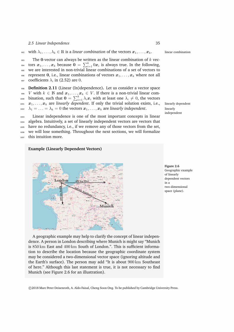
Figure 2.6Geographic exampleof linearlydependent vectorsin atwo-dimensionalspace (plane).

900 kmSoutheast

London

Munich

400km

South

850 km East

A geographic example may help to clarify the concept of linear indepen-dence. A person in London describing where Munich is might say “Munichis 850 km East and 400 km South of London.”. This is sufficient informa-tion to describe the location because the geographic coordinate systemmay be considered a two-dimensional vector space (ignoring altitude andthe Earth’s surface). The person may add “It is about 900 km Southeastof here.” Although this last statement is true, it is not necessary to findMunich (see Figure 2.6 for an illustration).


36 Linear Algebra

In this example, the “400 km South” vector and the “850 km East” vec-tor are linearly independent. That is to say, the South vector cannot bedescribed in terms of the East vector, and vice versa. However, the third“900 km Southeast” vector is a linear combination of the other two vec-tors, and it makes the set of vectors linearly dependent, i.e., one of thethree vectors is unnecessary.

Remark. The following properties are useful to find out whether vectors1008

are linearly independent.1009

• k vectors are either linearly dependent or linearly independent. There1010

is no third option.1011

• If at least one of the vectors x1, . . . ,xk is 0 then they are linearly de-1012

pendent. The same holds if two vectors are identical.1013

• The vectors {x1, . . . ,xk : xi 6= 0, i = 1, . . . , k}, k > 2, are linearly1014

dependent if and only if (at least) one of them is a linear combination1015

of the others. In particular, if one vector is a multiple of another vector,1016

i.e., xi = λxj, λ ∈ R then the set {x1, . . . ,xk : xi 6= 0, i = 1, . . . , k}1017

is linearly dependent.1018

• A practical way of checking whether vectors x1, . . . ,xk ∈ V are linearly1019

independent is to use Gaussian elimination: Write all vectors as columns1020

of a matrix A. Gaussian elimination yields a matrix in (reduced) row1021

echelon form.1022

– The pivot columns indicate the vectors, which are linearly indepen-1023

dent of the previous vectors, i.e., the vectors on the left. Note that1024

there is an ordering of vectors when the matrix is built.1025

– The non-pivot columns can be expressed as linear combinations ofthe pivot columns on their left. For instance, in[

1 3 00 0 1

](2.53)

the first and third column are pivot columns. The second column is a1026

non-pivot column because it is 3 times the first column.1027

If all columns are pivot columns, the column vectors are linearly inde-1028

pendent. If there is at least one non-pivot column, the columns (and,1029

therefore, the corresponding vectors) are linearly dependent.1030

♦1031

ExampleConsider R4 with

x1 =

12−34

, x2 =

1102

, x3 =

−1−211

. (2.54)


http://mml-book.com

2.5 Linear Independence 37

To check whether they are linearly dependent, we follow the general ap-proach and solve

λ1x1 + λ2x2 + λ3x3 = λ1

12−34

+ λ2

1102

+ λ3

−1−211

= 0 (2.55)

for λ1, . . . , λ3. We write the vectors xi, i = 1, 2, 3, as the columns of amatrix and apply elementary row operations until we identify the pivotcolumns:

1 1 −12 1 −2−3 0 14 2 1

· · ·

1 1 −10 1 00 0 10 0 0

(2.56)

Here, every column of the matrix is a pivot column. Therefore, there is nonon-trivial solution, and we require λ1 = 0, λ2 = 0, λ3 = 0 to solve theequation system. Hence, the vectors x1,x2,x3 are linearly independent.

Remark. Consider a vector space V with k linearly independent vectorsb1, . . . , bk and m linear combinations

x1 =k∑i=1

λi1bi ,

...

xm =k∑i=1

λimbi .

(2.57)

Defining B = (b1| . . . |bk) as the matrix whose columns are the linearlyindependent vectors b1, . . . , bk, we can write

xj = Bλj , λj =

λ1j

...λkj

, j = 1, . . . ,m , (2.58)

in a more compact form.1032

We want to test whether x1, . . . ,xm are linearly independent. For thispurpose, we follow the general approach of testing when

∑mj=1 ψjxj = 0.

With (2.58), we obtainm∑j=1

ψjxj =m∑j=1

ψjBλj = Bm∑j=1

ψjλj . (2.59)


38 Linear Algebra

This means that {x1, . . . ,xm} are linearly independent if and only if the1033

column vectors {λ1, . . . ,λm} are linearly independent.1034

♦1035

Remark. In a vector space V ,m linear combinations of k vectors x1, . . . ,xk1036

are linearly dependent if m > k. ♦1037

ExampleConsider a set of linearly independent vectors b1, b2, b3, b4 ∈ Rn and

x1 = b1 − 2b2 + b3 − b4

x2 = −4b1 − 2b2 + 4b4

x3 = 2b1 + 3b2 − b3 − 3b4

x4 = 17b1 − 10b2 + 11b3 + b4

(2.60)

Are the vectors x1, . . . ,x4 ∈ Rn linearly independent? To answer thisquestion, we investigate whether the column vectors

1−21−1

,−4−204

,

23−1−3

,

17−10111

(2.61)

are linearly independent. The reduced row echelon form of the corre-sponding linear equation system with coefficient matrix

A =

1 −4 2 17−2 −2 3 −101 0 −1 11−1 4 −3 1

(2.62)

is given as 1 0 0 −70 1 0 −150 0 1 −180 0 0 0

. (2.63)

We see that the corresponding linear equation system is non-trivially solv-able: The last column is not a pivot column, and x4 = −7x1−15x2−18x3.Therefore, x1, . . . ,x4 are linearly dependent as x4 can be expressed as alinear combination of x1, . . . ,x3.

2.6 Basis and Rank1038

In a vector space V , we are particularly interested in sets of vectors A that1039

possess the property that any vector v ∈ V can be obtained by a linear1040

combination of vectors in A. These vectors are special vectors, and in the1041

following, we will characterize them.1042


http://mml-book.com

2.6 Basis and Rank 39

2.6.1 Generating Set and Basis1043

Definition 2.12 (Generating Set/Span). Consider a vector space V and1044

set of vectors A = {x1, . . . ,xk} ⊆ V . If every vector v ∈ V can be1045

expressed as a linear combination of x1, . . . ,xk, A is called a generating generating set1046

set or span, which spans the vector space V . In this case, we write V = [A] span1047

or V = [x1, . . . ,xk].1048

Generating sets are sets of vectors that span vector (sub)spaces, i.e.,1049

every vector can be represented as a linear combination of the vectors1050

in the generating set. Now, we will be more specific and characterize the1051

smallest generating set that spans a vector (sub)space.1052

Definition 2.13 (Basis). Consider a real vector space V and A ⊆ V .1053

• A generating set A of V is called minimal if there exists no smaller set minimal1054

A ⊆ A ⊆ V that spans V .1055

• Every linearly independent generating set of V is minimal and is called1056

a basis of V . basis1057

Let V be a real vector space and B ⊆ V,B 6= ∅. Then, the following1058

statements are equivalent:1059

• B is a basis of V1060

• B is a minimal generating set1061

• B is a maximal linearly independent subset of vectors in V .1062

• Every vector x ∈ V is a linear combination of vectors from B, and everylinear combination is unique, i.e., with

x =k∑i=1

λibi =k∑i=1

ψibi (2.64)

and λi, ψi ∈ R, bi ∈ B it follows that λi = ψi, i = 1, . . . , k.1063

Example

• In R3, the canonical/standard basis is canonical/standardbasis

B =

1

00

,0

10

,0

01

. (2.65)

• Different bases in R3 are

B1 =

1

00

,1

10

,1

11

, B2 =

0.5

0.8−0.4

,1.8

0.30.3

,−2.2−1.33.5

(2.66)


40 Linear Algebra

• The set

A =

1234

,

2−102

,

110−4

(2.67)

is linearly independent, but not a generating set (and no basis) of R4:For instance, the vector [1, 0, 0, 0]> cannot be obtained by a linear com-bination of elements in A.

Remark. Every vector space V possesses a basis B. The examples above1064

show that there can be many bases of a vector space V , i.e., there is no1065

unique basis. However, all bases possess the same number of elements,1066

the basis vectors. ♦basis vectors 1067

We only consider finite-dimensional vector spaces V . In this case, the1068

dimension of V is the number of basis vectors, and we write dim(V ). Ifdimension 1069

U ⊆ V is a subspace of V then dim(U) 6 dim(V ) and dim(U) = dim(V )1070

if and only if U = V . Intuitively, the dimension of a vector space can be1071

thought of as the number of independent directions in this vector space.1072

Remark. A basis of a subspace U = [x1, . . . ,xm] ⊆ Rn can be found by1073

executing the following steps:1074

1. Write the spanning vectors as columns of a matrix A1075

2. Determine the row echelon form ofA, e.g., by means of Gaussian elim-1076

ination.1077

3. The spanning vectors associated with the pivot columns form a basis of1078

U .1079

♦1080

Example (Determining a Basis)For a vector subspace U ⊆ R5, spanned by the vectors

x1 =

12−1−1−1

, x2 =

2−112−2

, x3 =

3−435−3

, x4 =

−18−5−61

∈ R5,

(2.68)

we are interested in finding out which vectors x1, . . . ,x4 are a basis for U .For this, we need to check whether x1, . . . ,x4 are linearly independent.


http://mml-book.com

2.6 Basis and Rank 41

Therefore, we need to solve4∑i=1

λixi = 0 , (2.69)

which leads to a homogeneous equation system with the correspondingmatrix

[x1|x2|x3|x4

]=

1 2 3 −12 −1 −4 8−1 1 3 −5−1 2 5 −6−1 −2 −3 1

. (2.70)

With the basic transformation of linear equation systems, we obtain1 2 3 −12 −1 −4 8−1 1 3 −5−1 2 5 −6−1 −2 −3 1

· · ·

1 0 −1 00 1 2 00 0 0 10 0 0 00 0 0 0

.

From this reduced-row echelon form we see that x1,x2,x4 belong to thepivot columns, and, therefore, are linearly independent (because the lin-ear equation system λ1x1 + λ2x2 + λ4x4 = 0 can only be solved withλ1 = λ2 = λ4 = 0). Therefore, {x1,x2,x4} is a basis of U .

2.6.2 Rank1081

The number of linearly independent columns of a matrix A ∈ Rm×n1082

equals the number of linearly independent rows and is called the rank rank1083

of A and is denoted by rk(A).1084

Remark. The rank of a matrix has some important properties:1085

• rk(A) = rk(A>), i.e., the column rank equals the row rank.1086

• The columns of A ∈ Rm×n span a subspace U ⊆ Rm with dim(U) =1087

rk(A).5 A basis of U can be found by applying Gaussian elimination to1088

A to identify the pivot columns.1089

• The rows of A ∈ Rm×n span a subspace W ⊆ Rn with dim(W ) =1090

rk(A). A basis of W can be found by applying Gaussian elimination to1091

A>.1092

• For allA ∈ Rn×n holds:A is regular (invertible) if and only if rk(A) =1093

n.1094

• For all A ∈ Rm×n and all b ∈ Rm it holds that the linear equation1095

5Later, we will call this subspace the image or range.


42 Linear Algebra

system Ax = b can be solved if and only if rk(A) = rk(A|b), where1096

A|b denotes the augmented system.1097

• For A ∈ Rm×n the subspace of solutions for Ax = 0 possesses dimen-1098

sion n− rk(A).61099

• A matrix A ∈ Rm×n has full rank if its rank equals the largest possiblefull rank 1100

rank for a matrix of the same dimensions. This means that the rank of1101

a full-rank matrix is the lesser of the number of rows and columns, i.e.,1102

rk(A) = min(m,n). A matrix is said to be rank deficient if it does notrank deficient 1103

have full rank.1104

♦1105

Example (Rank)

• A =

1 0 10 1 10 0 0

. A possesses two linearly independent rows (and

columns). Therefore, rk(A) = 2.

• A =

[1 2 34 8 12

]. We see that the second row is a multiple of the first

row, such that the reduced row-echelon form of A is[1 2 30 0 0

], and

rk(A) = 1.

• A =

1 2 1−2 −3 13 5 0

We use Gaussian elimination to determine the

rank: 1 2 1−2 −3 13 5 0

· · ·

1 2 10 −1 30 0 0

(2.71)

Here, we see that the number of linearly independent rows and columnsis 2, such that rk(A) = 2.

2.7 Linear Mappings1106

In the following, we will study mappings on vector spaces that preservetheir structure. In the beginning of the chapter, we said that vectors areobjects that can be added together and multiplied by a scalar, and theresulting object is still a vector. This property we wish to preserve when

6Later, we will call this subspace the kernel or the nullspace.


http://mml-book.com

2.7 Linear Mappings 43

applying the mapping: Consider two real vector spaces V,W . A mappingΦ : V →W preserves the structure of the vector space if

Φ(x+ y) = Φ(x) + Φ(y) (2.72)

Φ(λx) = λΦ(x) (2.73)

for all x,y ∈ V and λ ∈ R. We can summarize this in the following1107

definition:1108

Definition 2.14 (Linear Mapping). For real vector spaces V,W , a map-ping Φ : V → W is called a linear mapping (or vector space homomor- linear mapping

vector spacehomomorphism

phism/linear transformation) if

lineartransformation

∀x,y ∈ V ∀λ, ψ ∈ R : Φ(λx+ ψy) = λΦ(x) + ψΦ(y) . (2.74)

Important special cases of linear mappings are1109

Isomorphism• Isomorphism: Φ : V →W linear and bijective1110 Endomorphism• Endomorphism: Φ : V → V linear1111 Automorphism• Automorphism: Φ : V → V linear and bijective1112

• We define idV : V → V , x 7→ x as the identity mapping in V . identity mapping1113

Example (Homomorphism)The mapping Φ : R2 → C, Φ(x) = x1 + ix2, is a homomorphism:

Φ

([x1

x2

]+

[y1

y2

])= (x1 + y1) + i(x2 + y2) = x1 + ix2 + y1 + iy2

= Φ

([x1

x2

])+ Φ

([y1

y2

])Φ

(λ

[x1

x2

])= λx1 + λix2 = λ(x1 + ix2) = λΦ

([x1

x2

])(2.75)

This also justifies why complex numbers can be represented as tuples inR2: There is a bijective linear mapping7 that converts the elementwiseaddition of tuples in R2 into the set of complex numbers with the corre-sponding addition.

Theorem 2.15. Finite-dimensional vector spaces V and W are isomorphic1114

if and only if dim(V ) = dim(W ).1115

Theorem 2.15 states that there exists a linear, bijective mapping be-1116

tween two vector spaces of the same dimension. Intuitively, this means1117

that vector spaces of the same dimension are kind of the same thing as1118

they can be transformed into each other without incurring any loss.1119

Theorem 2.15 also gives us the justification to treat Rm×n (the vector1120

space of m × n-matrices) and Rmn (the vector space of vectors of length1121

mn) the same as their dimensions are mn, and there exists a linear, bijec-1122

tive mapping that transforms one into the other.1123


44 Linear Algebra

2.7.1 Matrix Representation of Linear Mappings1124

Any n-dimensional vector space is isomorphic to Rn (Theorem 2.15). Weconsider now a basis {b1, . . . , bn} of an n-dimensional vector space V . Inthe following, the order of the basis vectors will be important. Therefore,we write

B = (b1, . . . , bn) (2.76)

and call this n-tuple an ordered basis of V .ordered basis 1125

Definition 2.16 (Coordinates). Consider a vector space V and an orderedbasis B = (b1, . . . , bn) of V . For any x ∈ V we obtain a unique represen-tation (linear combination)

x = α1b1 + . . .+ αnbn (2.77)

of x with respect to B. Then α1, . . . , αn are the coordinates of x withcoordinates

respect to B, and the vector α1

...αn

∈ Rn (2.78)

is the coordinate vector/coordinate representation of x with respect to thecoordinate vectorcoordinaterepresentation

1126

ordered basis B.1127

Figure 2.7Different Coordinaterepresentations of avector. Thecoordinates of thevector x are thecoefficients of thelinear combinationof the basis vectors.Depending on thechoice of basis, thecoordinates differ.

e1

e2 b2

b1

x = −12b1 +

52b2

x = 2e1 + 3e2

Remark. Intuitively, the basis vectors can be understood as units (includ-ing rather odd units such as “apples”, “bananas”, “kilograms” or “sec-onds”). Let us have a look at a geometric vector x ∈ R2 with coordinates[

23

](2.79)

with respect to the standard basis e1, e2 in R2. This means, we can writex = 2e1 + 3e2. However, we do not have to choose the standard basis torepresent this vector. If we use the basis vectors b1 = [1,−1]>, b2 = [1, 1]>

we will obtain the coordinates1

2

[−15

](2.80)

to represent the same vector (see Figure 2.7). ♦1128

In the following, we will look at mappings that transform coordinate1129

vectors with respect to one basis into coordinate vectors with respect to a1130

different basis.1131

Remark. For an n-dimensional vector space V and an ordered basis B1132

of V , the mapping Φ : Rn → V , Φ(ei) = bi, i = 1, . . . , n, is linear1133

(and because of Theorem 2.15 an isomorphism), where (e1, . . . , en) is1134

the standard basis of Rn.1135

♦1136


http://mml-book.com


Now we are ready to make an explicit connection between matrices and1137

linear mappings between finite-dimensional vector spaces.1138

Definition 2.17 (Transformation matrix). Consider vector spaces V,Wwith corresponding (ordered) bases = (b1, . . . , bn) and C = (c1, . . . , cm).Moreover, we consider a linear mapping Φ : V →W . For j ∈ {1, . . . , n}

Φ(bj) = α1jc1 + · · ·+ αmjcm =m∑i=1

αijci (2.81)

is the unique representation of Φ(bj) with respect to C. Then, we call them× n-matrix

AΦ := ((αij)) (2.82)

the transformation matrix of Φ (with respect to the ordered bases B of V transformationmatrix

1139

and C of W ).1140

The coordinates of Φ(bj) with respect to the ordered basis C of Ware the j-th column of AΦ, and rk(AΦ) = dim(Im(Φ)). Consider (finite-dimensional) vector spaces V,W with ordered bases B,C and a linearmapping Φ : V →W with transformation matrix AΦ. If x is the coordi-nate vector of x ∈ V with respect to B and y the coordinate vector ofy = Φ(x) ∈W with respect to C, then

y = AΦx . (2.83)

This means that the transformation matrix can be used to map coordinates1141

with respect to an ordered basis in V to coordinates with respect to an1142

ordered basis in W .1143

Example (Transformation Matrix)Consider a homomorphism Φ : V → W and ordered bases B =(b1, . . . , b3) of V and C = (c1, . . . , c4) of W . With

Φ(b1) = c1 − c2 + 3c3 − c4

Φ(b2) = 2c1 + c2 + 7c3 + 2c4

Φ(b3) = 3c2 + c3 + 4c4

(2.84)

the transformation matrix AΦ with respect to B and C satisfies Φ(bk) =∑4i=1 αikci for k = 1, . . . , 3 and is given as

AΦ = (α1|α2|α3) =

1 2 0−1 1 33 7 1−1 2 4

, (2.85)

where the αj, j = 1, 2, 3, are the coordinate vectors of Φ(bj) with respectto C.


46 Linear AlgebraFigure 2.8 Threeexamples of lineartransformations ofthe vectors shownin (a). (b) Rotationby 45◦; (c)Stretching of thehorizontalcoordinates by 2;(d) Combination ofreflection, rotationand stretching.

(a) Original data. (b) Rotation by 45◦. (c) Stretch along thehorizontal axis.

(d) General linear map-ping.

Example (Linear Transformations of Vectors)We consider three linear transformations of a set of vectors in R2 with thetransformation matrices

A1 =

[cos(π

4) − sin(π

4)

sin(π4) cos(π

4)

], A2 =

[2 00 1

], A3 =

1

2

[3 −11 −1

].

(2.86)

Figure 2.8 gives three examples of linear transformations of a set ofvectors. Figure 2.8(a) shows 400 vectors in R2, each of which is repre-sented by a dot at the corresponding (x1, x2)-coordinates. The vectors arearranged in a square. When we use matrix A1 in (2.86) to linearly trans-form each of these vectors, we obtain the rotated square in Figure 2.8(b).If we apply the linear mapping represented byA2, we obtain the rectanglein Figure 2.8(c) where each x1-coordinate is stretched by 2. Figure 2.8(d)shows the original square from Figure 2.8(a) when linearly transformedusing A3, which is a combination of a reflection, a rotation and a stretch.

2.7.2 Basis Change1144

In the following, we will have a closer look at how transformation matricesof a linear mapping Φ : V → W change if we change the bases in V andW . Consider two ordered bases

B = (b1, . . . , bn), B = (b1, . . . , bn) (2.87)

of V and two ordered bases

C = (c1, . . . , cm), C = (c1, . . . , cm) (2.88)

of W . Moreover, AΦ ∈ Rm×n is the transformation matrix of the linear1145

mapping Φ : V →W with respect to the bases B and C, and AΦ ∈ Rm×n1146

is the corresponding transformation mapping with respect to B and C.1147

We will now investigate how A and A are related, i.e., how/whether we1148

can transform AΦ into AΦ if we choose to perform a basis change from1149

B,C to B, C.1150


http://mml-book.com


Remark. We effectively get different coordinate representations of the1151

identity mapping idV . In the context of Figure 2.7, this would mean to1152

map coordinates with respect to e1, e2 onto coordinates with respect to1153

b1, b2 without changing the vector x. ♦1154

We can now write the vectors of the new basis B of V as a linear com-bination of the basis vectors of B, such that

bj = s1jb1 + · · ·+ snjbn =n∑i=1

sijbi , j = 1, . . . , n . (2.89)

Similarly, we write the new basis vectors C of W as a linear combinationof the basis vectors of C, which yields

ck = t1kc1 + · · ·+ tmkcm =m∑l=1

tlkcl , k = 1, . . . ,m . (2.90)

We define S = ((sij)) ∈ Rn×n as the transformation matrix that maps1155

coordinates with respect to B onto coordinates with respect to B, and1156

T = ((tlk)) ∈ Rm×m as the transformation matrix that maps coordinates1157

with respect to C onto coordinates with respect to C. In particular, the1158

jth column of S are the coordinate representations of bj with respect to1159

B and the jth columns of T is the coordinate representation of cj with1160

respect to C. Note that both S and T are regular.1161

For all j = 1, . . . , n, we get

Φ(bj) =m∑k=1

akj ck︸︷︷︸∈W

(2.90)=

m∑l=1

akj

m∑l=1

tlkcl =m∑l=1

(m∑k=1

tlkakj

)cl , (2.91)

where we first expressed the new basis vectors ck ∈W as linear combina-tions of the basis vectors cl ∈ W and then swapped the order of summa-tion. When we express the bj ∈ V as linear combinations of bj ∈ V , wearrive at

Φ(bj)(2.89)= Φ

(n∑i=1

sijbi

)=

n∑i=1

sijΦ(bi) =n∑i=1

sij

m∑l=1

alicl (2.92)

=m∑l=1

(n∑i=1

alisij

)cl , j = 1, . . . , n , (2.93)

where we exploited the linearity of Φ. Comparing (2.91) and (2.93), itfollows for all j = 1, . . . , n and l = 1, . . . ,m that

m∑k=1

tlkakj =n∑i=1

alisij (2.94)

and, therefore,

TAΦ = AΦS ∈ Rm×n , (2.95)


48 Linear Algebra

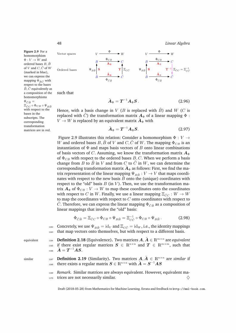
Figure 2.9 For ahomomorphismΦ : V →W andordered bases B, Bof V and C, C of W(marked in blue),we can express themapping ΦBC withrespect to the basesB, C equivalently asa composition of thehomomorphismsΦCB =

ΞCC ◦ ΦCB ◦ΨBBwith respect to thebases in thesubscripts. Thecorrespondingtransformationmatrices are in red.

V W

B

B C

C

Φ

ΦCB

ΦCB

ΨBB ΞCCS T

AΦ

AΦ

V W

B

B C

C

Φ

ΦCB

ΦCB

ΨBB ΞCC = Ξ−1

CCS T−1

AΦ

AΦ

Vector spaces

Ordered bases

such that

AΦ = T−1AΦS . (2.96)

Hence, with a basis change in V (B is replaced with B) and W (C isreplaced with C) the transformation matrix AΦ of a linear mapping Φ :V →W is replaced by an equivalent matrix AΦ with

AΦ = T−1AΦS. (2.97)

Figure 2.9 illustrates this relation: Consider a homomorphism Φ : V →W and ordered bases B, B of V and C, C of W . The mapping ΦCB is aninstantiation of Φ and maps basis vectors of B onto linear combinationsof basis vectors of C. Assuming, we know the transformation matrix AΦ

of ΦCB with respect to the ordered bases B,C. When we perform a basischange from B to B in V and from C to C in W , we can determine thecorresponding transformation matrix AΦ as follows: First, we find the ma-trix representation of the linear mapping ΨBB : V → V that maps coordi-nates with respect to the new basis B onto the (unique) coordinates withrespect to the “old” basis B (in V ). Then, we use the transformation ma-trix AΦ of ΦCB : V → W to map these coordinates onto the coordinateswith respect to C in W . Finally, we use a linear mapping ΞCC : W → Wto map the coordinates with respect to C onto coordinates with respect toC. Therefore, we can express the linear mapping ΦCB as a composition oflinear mappings that involve the “old” basis:

ΦCB = ΞCC ◦ ΦCB ◦ΨBB = Ξ−1

CC◦ ΦCB ◦ΨBB . (2.98)

Concretely, we use ΨBB = idV and ΞCC = idW , i.e., the identity mappings1162

that map vectors onto themselves, but with respect to a different basis.1163

Definition 2.18 (Equivalence). Two matricesA, A ∈ Rm×n are equivalentequivalent 1164

if there exist regular matrices S ∈ Rn×n and T ∈ Rm×m, such that1165

A = T−1AS.1166

Definition 2.19 (Similarity). Two matrices A, A ∈ Rn×n are similar ifsimilar 1167

there exists a regular matrix S ∈ Rn×n with A = S−1AS1168

Remark. Similar matrices are always equivalent. However, equivalent ma-1169

trices are not necessarily similar. ♦1170


http://mml-book.com


Remark. Consider vector spaces V,W,X. From Remark 2.7.3 we already1171

know that for linear mappings Φ : V →W and Ψ : W → X the mapping1172

Ψ ◦ Φ : V → X is also linear. With transformation matrices AΦ and AΨ1173

of the corresponding mappings, the overall transformation matrix AΨ◦Φ1174

is given by AΨ◦Φ = AΨAΦ. ♦1175

In light of this remark, we can look at basis changes from the perspec-1176

tive of composing linear mappings:1177

• AΦ is the transformation matrix of a linear mapping ΦCB : V → W1178

with respect to the bases B,C.1179

• AΦ is the transformation matrix of the linear mapping ΦCB : V → W1180

with respect to the bases B, C.1181

• S is the transformation matrix of a linear mapping ΨBB : V → V1182

(automorphism) that represents B in terms of B. Normally, Ψ = idV is1183

the identity mapping in V .1184

• T is the transformation matrix of a linear mapping ΞCC : W → W1185

(automorphism) that represents C in terms of C. Normally, Ξ = idW is1186

the identity mapping in W .1187

If we (informally) write down the transformations just in terms of basesthen AΦ : B → C, AΦ : B → C, S : B → B, T : C → C andT−1 : C → C, and

B → C = B → B→ C → C (2.99)

AΦ = T−1AΦS . (2.100)

Note that the execution order in (2.100) is from right to left because vec-1188

tors are multiplied at the right-hand side so that x 7→ Sx 7→ AΦ(Sx) 7→1189

T−1(AΦ(Sx)

)= AΦx.1190

Example (Basis Change)Consider a linear mapping Φ : R3 → R4 whose transformation matrix is

AΦ =

1 2 0−1 1 33 7 1−1 2 4

(2.101)

with respect to the standard bases

B = (

100

,0

10

,0

01

) , C = (

1000

,

0100

,

0010

,

0001

). (2.102)

We seek the transformation matrix AΦ of Φ with respect to the new bases


50 Linear Algebra

B = (

110

,0

11

,1

01

) ∈ R3, C = (

1100

,

1010

,

0110

,

1001

) . (2.103)

Then,

S =

1 0 11 1 00 1 1

, T =

1 1 0 11 0 1 00 1 1 00 0 0 1

, (2.104)

where the ith column of S is the coordinate representation of bi in termsof the basis vectors of B.8 Similarly, the jth column of T is the coordinaterepresentation of cj in terms of the basis vectors of C.

Therefore, we obtain

AΦ = T−1AΦS =

1/2 1/2 −1/2 −1/21/2 −1/2 1/2 −1/2−1/2 1/2 1/2 1/2

0 0 0 1

3 2 10 4 210 8 41 6 3

(2.105)

=

−4 −4 −26 0 04 8 41 6 3

. (2.106)

In Chapter 4, we will be able to exploit the concept of a basis change1191

to find a basis with respect to which the transformation matrix of an en-1192

domorphism has a particularly simple (diagonal) form. In Chapter 11, we1193

will look at a data compression problem and find a convenient basis onto1194

which we can project the data while minimizing the compression loss.1195

2.7.3 Image and Kernel1196

The image and kernel of a linear mapping are vector subspaces with cer-1197

tain important properties. In the following, we will characterize them1198

more carefully.1199

Definition 2.20 (Image and Kernel).1200

For Φ : V →W , we define the kernel/null spacekernelnull space

ker(Φ) := Φ−1({0W}) = {v ∈ V : Φ(v) = 0W} (2.107)

and the image/rangeimagerange

Im(Φ) := Φ(V ) = {w ∈W |∃v ∈ V : Φ(v) = w} . (2.108)


http://mml-book.com


Figure 2.10 Kerneland Image of alinear mappingΦ : V →W .

V WΦ : V → W

Im(Φ)Ker(Φ)

00

Intuitively, the kernel is the set of vectors in v ∈ V that Φ maps onto1201

the neutral element 0W ∈W . The image is the set of vectors w ∈W that1202

can be “reached” by Φ from any vector in V . An illustration is given in1203

Figure 2.10.1204

Remark. Consider a linear mapping Φ : V → W , where V,W are vector1205

spaces.1206

• It always holds that Φ({0V }) = 0W and, therefore, 0V ∈ ker(Φ). In1207

particular, the null space is never empty.1208

• Im(Φ) ⊆W is a subspace of W , and ker(Φ) ⊆ V is a subspace of V .1209

• Φ is injective (one-to-one) if and only if ker(Φ) = {0}1210

♦1211

Remark (Null Space and Column Space). Let us consider A ∈ Rm×n and1212

a linear mapping Φ : Rn → Rm, x 7→ Ax.1213

• For A = (a1|...|an), where ai are the columns of A, we obtain

Im(Φ) = {Ax : x ∈ Rn} = {x1a1 + ...+ xnan : x1, . . . , xn ∈ R}(2.109)

= [a1, . . . ,an] ⊆ Rm , (2.110)

i.e., the image is the span of the columns of A, also called the column column space1214

space. Therefore, the column space (image) is a subspace of Rm, where1215

m is the “height” of the matrix.1216

• The kernel/null space ker(Φ) is the general solution to the linear ho-1217

mogeneous equation system Ax = 0 and captures all possible linear1218

combinations of the elements in Rn that produce 0 ∈ Rm.1219

• The kernel is a subspace of Rn, where n is the “width” of the matrix.1220

• The kernel focuses on the relationship among the columns, and we can1221

use it to determine whether/how we can express a column as a linear1222

combination of other columns.1223

• The purpose of the kernel is to determine whether a solution of the1224

linear equation system is unique and, if not, to capture all possible so-1225

lutions.1226


52 Linear Algebra

♦1227

Example (Image and Kernel of a Linear Mapping)The mapping

Φ : R4 → R2,

x1

x2

x3

x4

7→ [1 2 −1 01 0 0 1

]x1

x2

x3

x4

=

[x1 + 2x2 − x3

x1 + x4

](2.111)

= x1

[11

]+ x2

[20

]+ x3

[−10

]+ x4

[01

](2.112)

is linear. To determine Im(Φ) we can simply take the span of the columnsof the transformation matrix and obtain

Im(Φ) = [

[11

],

[20

],

[−10

],

[01

]]. (2.113)

To compute the kernel (null space) of Φ, we need to solve Ax = 0, i.e.,we need to solve a homogeneous equation system. To do this, we useGaussian elimination to transform A into reduced row echelon form:[

1 2 −1 01 0 0 1

] · · ·

[1 0 0 10 1 − 1

2− 1

2

](2.114)

This matrix is now in reduced row echelon form, and we can now usethe Minus-1 Trick to compute a basis of the kernel (see Section 2.3.3).Alternatively, we can express the non-pivot columns (columns 3 and 4)as linear combinations of the pivot-columns (columns 1 and 2). The thirdcolumn a3 is equivalent to − 1

2times the second column a2. Therefore,

0 = a3 + 12a2. In the same way, we see that a4 = a1− 1

2a2 and, therefore,

0 = a1 − 12a2 − a4. Overall, this gives us now the kernel (null space) as

ker(Φ) = [

012

10

,−1

12

01

]. (2.115)

Theorem 2.21 (Rank-Nullity Theorem). For vector spaces V,W and a lin-ear mapping Φ : V →W it holds that

dim(ker(Φ)) + dim(Im(Φ)) = dim(V ) (2.116)

Remark. Consider vector spaces V,W,X. Then:1228

• For linear mappings Φ : V → W and Ψ : W → X the mapping1229

Ψ ◦ Φ : V → X is also linear.1230


http://mml-book.com

2.8 Affine Spaces 53

• If Φ : V →W is an isomorphism then Φ−1 : W → V is an isomorphism1231

as well.1232

• If Φ : V → W, Ψ : V → W are linear then Φ + Ψ and λΦ, λ ∈ R are1233

linear, too.1234

♦1235

2.8 Affine Spaces1236

In the following, we will have a closer look at spaces that are offset from1237

the origin, i.e., spaces that are no longer vector subspaces. Moreover, we1238

will briefly discuss properties of mappings between these affine spaces,1239

which resemble linear mappings.1240

2.8.1 Affine Subspaces1241

Definition 2.22 (Affine Subspace). Let V be a vector space, x0 ∈ V andU ⊆ V a subspace. Then the subset

L = x0 + U := {x0 + u : u ∈ U} = {v ∈ V |∃u ∈ U : v = x0 + u} ⊆ V(2.117)

is called affine subspace or linear manifold of V . U is called direction or affine subspace

linear manifolddirection

1242

direction space, and x0 is called support point. In Chapter 10 we refer to

direction space

support point

1243

these subspaces as hyperplanes.1244

Note that the definition of an affine subspace excludes 0 if x0 /∈ U .1245

Therefore, an affine subspace is not a (linear) subspace (vector subspace)1246

of V for x0 /∈ U .1247

Examples of affine subspaces are points, lines and planes in R3, which1248

do not (necessarily) go through the origin.1249

Remark. Consider two affine subspaces L = x0 +U and L = x0 + U of a1250

vector space V . Then, L ⊆ L if and only if U ⊆ U and x0 − x0 ∈ U .1251

Affine subspaces are often described by parameters: Consider a k-dimen- parameters

sional affine space L = x0 + U of V . If (b1, . . . , bk) is an ordered basis ofU , then every element x ∈ L can be (uniquely) described as

x = x0 + λ1b1 + . . .+ λkbk , (2.118)

where λ1, . . . , λk ∈ R. This representation is called parametric equation parametric equation1252

of L with directional vectors b1, . . . , bk and parameters λ1, . . . , λk. ♦ parameters1253

Example (Affine Subspaces)


54 Linear Algebra

Figure 2.11 Vectorsy on a line lie in anaffine subspace Lwith support pointx0 and direction u.

0

x0

u

y

L = x0 + λu

• One-dimensional affine subspaces are called lines and can be writtenlines

as y = x0 + λx1, where λ ∈ R, where U = [x1] ⊆ Rn is a one-dimensional subspace of Rn. This means, a line is defined by a supportpoint x0 and a vector x1 that defines the direction. See Figure 2.11 foran illustration.• Two-dimensional affine subspaces of Rn are called planes. The para-planes

metric equation for planes is y = x0 + λ1x1 + λ2x2, where λ1, λ2 ∈ Rand U = [x1,x2] ⊆ Rn. This means, a plane is defined by a supportpoint x0 and two linearly independent vectors x1,x2 that span the di-rection space.• In Rn, the (n− 1)-dimensional affine subspaces are called hyperplanes,hyperplanes

and the corresponding parametric equation is y = x0 +∑n−1

i=1 λixi,where x1, . . . ,xn−1 form a basis of an (n − 1)-dimensional subspaceU of Rn. This means, a hyperplane is defined by a support point x0

and (n − 1) linearly independent vectors x1, . . . ,xn−1 that span thedirection space. In R2, a line is also a hyperplane. In R3, a plane is alsoa hyperplane.

Remark (Inhomogeneous linear equation systems and affine subspaces).1254

For A ∈ Rm×n and b ∈ Rm the solution of the linear equation system1255

Ax = b is either the empty set or an affine subspace of Rn of dimension1256

n− rk(A). In particular, the solution of the linear equation λ1x1 + . . .+1257

λnxn = b, where (λ1, . . . , λn) 6= (0, . . . , 0), is a hyperplane in Rn.1258

In Rn, every k-dimensional affine subspace is the solution of a linear1259

inhomogeneous equation systemAx = b, whereA ∈ Rm×n, b ∈ Rm and1260

rk(A) = n − k. Recall that for homogeneous equation systems Ax = 01261

the solution was a vector subspace (not affine). ♦1262

2.8.2 Affine Mappings1263

Similar to linear mappings between vector spaces, which we discussed1264

in Section 2.7, we can define affine mappings between two affine spaces.1265

Linear and affine mappings are closely related. Therefore, many properties1266


http://mml-book.com

Exercises 55

that we already know from linear mappings, e.g., that the composition of1267

linear mappings is a linear mapping, also hold for affine mappings.1268

Definition 2.23 (Affine mapping). For two vector spaces V,W and a lin-ear mapping Φ : V →W and a ∈W the mapping

φ :V →W (2.119)

x 7→ a+ Φ(x) (2.120)

is an affine mapping from V to W . The vector a is called translation vector affine mapping

translation vector

1269

of φ.1270

• Every affine mapping φ : V → W is also the composition of a linear1271

mapping Φ : V → W and a translation τ : W → W in W , such that1272

φ = τ ◦ Φ. The mappings Φ and τ are uniquely determined.1273

• The composition φ′ ◦ φ of affine mappings φ : V → W , φ′ : W → X is1274

affine.1275

• Affine mappings keep the geometric structure invariant. They also pre-1276

serve the dimension and parallelism.1277

Exercises1278

2.1 We consider (R\{−1}, ?) where where

a ? b := ab+ a+ b, a, b ∈ R\{−1} (2.121)

1. Show that (R\{−1}, ?) is an Abelian group1279

2. Solve

3 ? x ? x = 15

in the Abelian group (R\{−1}, ?), where ? is defined in (2.121).1280

2.2 Let n be inN \ {0}. Let k, x be in Z. We define the congruence class k of theinteger k as the set

k = {x ∈ Z | x− k = 0 (modn)}= {x ∈ Z | (∃a ∈ Z) : (x− k = n · a)} .

We now define Z/nZ (sometimes written Zn) as the set of all congruenceclasses modulo n. Euclidean division implies that this set is a finite set con-taining n elements:

Zn = {0, 1, . . . , n− 1}

For all a, b ∈ Zn, we define

a⊕ b := a+ b

1. Show that (Zn,⊕) is a group. Is it Abelian?1281


56 Linear Algebra

2. We now define another operation ⊗ for all a and b in Zn as

a⊗ b = a× b (2.122)

where a× b represents the usual multiplication in Z.1282

Let n = 5. Draw the times table of the elements of Z5 \ {0} under ⊗, i.e.,1283

calculate the products a⊗ b for all a and b in Z5 \ {0}.1284

Hence, show that Z5 \ {0} is closed under ⊗ and possesses a neutral1285

element for ⊗. Display the inverse of all elements in Z5 \ {0} under ⊗.1286

Conclude that (Z5 \ {0},⊗) is an Abelian group.1287

3. Show that (Z8 \ {0},⊗) is not a group.1288

4. We recall that Bezout theorem states that two integers a and b are rela-1289

tively prime (i.e., gcd(a, b) = 1, aka. coprime) if and only if there exist1290

two integers u and v such that au+ bv = 1. Show that (Zn \ {0},⊗) is a1291

group if and only if n ∈ N \ {0} is prime.1292

2.3 Consider the set G of 3× 3 matrices defined as:

G =

1 x z

0 1 y

0 0 1

∈ R3×3

∣∣∣∣∣∣x, y, z ∈ R (2.123)

We define · as the standard matrix multiplication.1293

Is (G, ·) a group ? If yes, is it Abelian ? Justify your answer.1294

2.4 Compute the following matrix products:1295

1. 1 2

4 5

7 8

1 1 0

0 1 1

1 0 1

2. 1 2 3

4 5 6

7 8 9

1 1 0

0 1 1

1 0 1

3. 1 1 0

0 1 1

1 0 1

1 2 3

4 5 6

7 8 9

4.

[1 2 1 2

4 1 −1 −4

]0 3

1 −1

2 1

5 2

5.

0 3

1 −1

2 1

5 2

[1 2 1 2

4 1 −1 −4

]


http://mml-book.com

Exercises 57

2.5 Find the set S of all solutions in x of the following inhomogeneous linear1296

systems Ax = b where A and b are defined below:1297

1.

A =

1 1 −1 −1

2 5 −7 −5

2 −1 1 3

5 2 −4 2

, b =

1

−2

4

6

2.

A =

1 −1 0 0 1

1 1 0 −3 0

2 −1 0 1 −1

−1 2 0 −2 −1

, b =

3

6

5

−1

3. Using Gaussian elimination find all solutions of the inhomogeneous equa-

tion system Ax = b with

A =

0 1 0 0 1 0

0 0 0 1 1 0

0 1 0 0 0 1

, b =

2

−1

1

2.6 Find all solutions in x =

x1

x2

x3

∈ R3 of the equation system Ax = 12x,

where

A =

6 4 3

6 0 9

0 8 0

and

∑3i=1 xi = 1.1298

2.7 Determine the inverse of the following matrices if possible:1299

1.

A =

2 3 4

3 4 5

4 5 6

2.

A =

1 0 1 0

0 1 1 0

1 1 0 1

1 1 1 0

Which of the following sets are subspaces of R3?1300

1. A = {(λ, λ+ µ3, λ− µ3) | λ, µ ∈ R}1301

2. B = {(λ2,−λ2, 0) | λ ∈ R}1302

3. Let γ be in R.1303

C = {(ξ1, ξ2, ξ3) ∈ R3 | ξ1 − 2ξ2 + 3ξ3 = γ}1304

4. D = {(ξ1, ξ2, ξ3) ∈ R3 | ξ2 ∈ Z}1305

2.8 Are the following vectors linearly independent?1306


58 Linear Algebra

1.

x1 =

2

−1

3

, x2

1

1

−2

, x3

3

−3

8

2.

x1 =

1

2

1

0

0

, x2 =

1

1

0

1

1

, x3 =

1

0

0

1

1

2.9 Write

y =

1

−2

5

as linear combination of

x1 =

1

1

1

, x2 =

1

2

3

, x3 =

2

−1

1

2.10 1. Determine a simple basis of U , where

U = [

1

1

1

1

,

2

3

4

1

,

3

4

5

3

] ⊆ R4

2. Consider two subspaces of R4:

U1 = [

1

1

−3

1

,

2

−1

0

−1

,−1

1

−1

1

] , U2 = [

−1

−2

2

1

,

2

−2

0

0

,−3

6

−2

−1

] .

Determine a basis of U1 ∩ U2.1307

3. Consider two subspaces U1 and U2, where U1 is the solution space of thehomogeneous equation system A1x = 0 and U2 is the solution space ofthe homogeneous equation system A2x = 0 with

A1 =

1 0 1

1 −2 −1

2 1 3

1 0 1

, A2 =

3 −3 0

1 2 3

7 −5 2

3 −1 2

.1. Determine the dimension of U1, U21308

2. Determine bases of U1 and U21309

3. Determine a basis of U1 ∩ U21310


http://mml-book.com

Exercises 59

2.11 Consider two subspaces U1 and U2, where U1 is spanned by the columns ofA1 and U2 is spanned by the columns of A2 with

A1 =

1 0 1

1 −2 −1

2 1 3

1 0 1

, A2 =

3 −3 0

1 2 3

7 −5 2

3 −1 2

.1. Determine the dimension of U1, U21311

2. Determine bases of U1 and U21312

3. Determine a basis of U1 ∩ U21313

2.12 Let F = {(x, y, z) ∈ R3 | x+y−z = 0} andG = {(a−b, a+b, a−3b) | a, b ∈ R}.1314

1. Show that F and G are subspaces of R3.1315

2. Calculate F ∩G without resorting to any basis vector.1316

3. Find one basis for F and one forG, calculate F∩G using the basis vectors1317

previously found and check your result with the previous question.1318

2.13 Are the following mappings linear?1319

1. Let a and b be in R.

φ : L1([a, b])→ R

f 7→ φ(f) =

∫ b

a

f(x)dx ,

where L1([a, b]) denotes the set of integrable function on [a, b].1320

2.

φ : C1 → C0

f 7→ φ(f) = f ′ .

where for k > 1, Ck denotes the set of k times continuously differentiable1321

functions, and C0 denotes the set of continuous functions.1322

3.

φ : R→ Rx 7→ φ(x) = cos(x)

4.

φ : R3 → R2

x 7→[1 2 3

1 4 3

]x

5. Let θ be in [0, 2π[.

φ : R2 → R2

x 7→[

cos(θ) sin(θ)

− sin(θ) cos(θ)

]x


60 Linear Algebra

2.14 Consider the linear mapping

Φ : R3 → R4

Φ

x1

x2

x3

=

3x1 + 2x2 + x3

x1 + x2 + x3

x1 − 3x2

2x1 + 3x2 + x3

• Find the transformation matrix AΦ1323

• Determine rk(AΦ)1324

• Compute kernel and image of Φ. What is dim(ker(Φ)) and dim(Im(Φ))?1325

2.15 Let E be a vector space. Let f and g be two endomorphisms on E such that1326

f◦g = idE (i.e. f◦g is the identity isomorphism). Show that ker f = ker(g◦f),1327

Img = Im(g ◦ f) and that ker(f) ∩ Im(g) = {0E}.1328

2.16 Consider an endomorphism Φ : R3 → R3 whose transformation matrix(with respect to the standard basis in R3) is

AΦ =

1 1 0

1 −1 0

1 1 1

.1. Determine ker(Φ) and Im(Φ).1329

2. Determine the transformation matrix AΦ with respect to the basis

B = (

1

1

1

,1

2

1

,1

0

0

) ,

i.e., perform a basis change toward the new basis B.1330

2.17 Let us consider four vectors b1, b2, b′1, b′2 of R2 expressed in the standard

basis of R2 as

b1 =

[2

1

], b2 =

[−1

−1

], b′1 =

[2

−2

], b′2 =

[1

1

](2.124)

and let us define B = (b1, b2) and B′ = (b′1, b′2).1331

1. Show that B and B′ are two bases of R2 and draw those basis vectors.1332

2. Compute the matrix P 1 which performs a basis change from B′ to B.1333

2.18 We consider three vectors c1, c2, c3 of R3 defined in the standard basis of R1334

as1335

c1 =

1

2

−1

, c2 =

0

−1

2

, c3 =

1

0

−1

(2.125)

and we define C = (c1, c2, c3).1336

1. Show that C is a basis of R3.1337

2. Let us call C′ = (c′1, c′2, c′3) the standard basis of R3. Explicit the matrix1338

P 2 that performs the basis change from C to C′.1339


http://mml-book.com

Exercises 61

2.19 Let us consider b1, b2, b′1, b′2, 4 vectors of R2 expressed in the standard basis

of R2 as

b1 =

[2

1

], b2 =

[−1

−1

], b′1 =

[2

−2

], b′2 =

[1

1

](2.126)

and let us define two ordered bases B = (b1, b2) and B′ = (b′1, b′2) of R2.1340

1. Show that B and B′ are two bases of R2 and draw those basis vectors.1341

2. Compute the matrix P 1 that performs a basis change from B′ to B.1342

3. We consider c1, c2, c3, 3 vectors of R3 defined in the standard basis of Ras

c1 =

1

2

−1

, c2 =

0

−1

2

, c3 =

1

0

−1

(2.127)

and we define C = (c1, c2, c3).1343

1. Show that C is a basis of R3 using determinants1344

2. Let us call C′ = (c′1, c′2, c′3) the standard basis of R3. Determine the1345

matrix P 2 that performs the basis change from C to C′.1346

4. We consider a homomorphism φ : R2 −→ R3, such that

φ(b1 + b2) = c2 + c3

φ(b1 − b2) = 2c1 − c2 + 3c3(2.128)

where B = (b1, b2) and C = (c1, c2, c3) are ordered bases of R2 and R3,1347

respectively.1348

Determine the transformation matrixAφ of φ with respect to the ordered1349

bases B and C.1350

5. Determine A′, the transformation matrix of φ with respect to the bases1351

B′ and C′.1352

6. Let us consider the vector x ∈ R2 whose coordinates in B′ are [2, 3]>. In1353

other words, x = 2b′1 + 3b′3.1354

1. Calculate the coordinates of x in B.1355

2. Based on that, compute the coordinates of φ(x) expressed in C.1356

3. Then, write φ(x) in terms of c′1, c′2, c′3.1357

4. Use the representation of x in B′ and the matrix A′ to find this result1358

directly.1359


linear algebra - mml-book.github.io · linear algebra 744 745 when formalizing ... therefore,...

Documents