linear and nonlinear rogue wave statistics in the presence ... · introduction tales of freak waves...

arX

iv:1

207.

2162

v1 [

nlin

.CD

] 9

Jul 2

012

Linear and Nonlinear Rogue Wave Statistics in the

Presence of Random Currents

L. H. Ying,1 Z. Zhuang2, E. J. Heller,3 and L. Kaplan,1

1Department of Physics and Engineering Physics, Tulane University, New Orleans,

Louisiana 70118, USA2School of Electrical and Computer Engineering, Cornell University, Ithaca, New

York 14853, USA3Department of Physics and Department of Chemistry and Chemical Biology,

Harvard University, Cambridge, Massachusetts 02138, USA

Abstract. We review recent progress in modeling the probability distribution of wave

heights in the deep ocean as a function of a small number of parameters describing

the local sea state. Both linear and nonlinear mechanisms of rogue wave formation are

considered. First, we show that when the average wave steepness is small and nonlinear

wave effects are subleading, the wave height distribution is well explained by a single

“freak index” parameter, which describes the strength of (linear) wave scattering by

random currents relative to the angular spread of the incoming random sea. When the

average steepness is large, the wave height distribution takes a very similar functional

form, but the key variables determining the probability distribution are the steepness,

and the angular and frequency spread of the incoming waves. Finally, even greater

probability of extreme wave formation is predicted when linear and nonlinear effects

are acting together.

http://arxiv.org/abs/1207.2162v1

Linear and Nonlinear Rogue Wave Statistics in the Presence of Random Currents 2

1. Introduction

Tales of freak waves by lucky survivors used to be taken with a large grain of salt. Were

the sailors making excuses for bad seamanship? The first such wave to be measured

directly was the famous New Year’s wave in 1995 [1]. With modern cameras and video,

not to mention satellites [2, 3], it is no longer controversial that freak or rogue extreme

waves exist on the world’s great oceans [4, 5, 6].

Any realistic seaway (an irregular, moderate to rough sea) is comprised of a

superposition of waves differing in wavelength and direction, with random relative

phases. Supposing that the dispersion in wavelengths is not too large, and assuming

uniform sampling, Longuet-Higgins [7] exploited the central limit theorem to derive a

large number of statistical properties of such wave superpositions, including of course

wave height distributions. From this viewpoint, extreme waves are the result of unlucky

coherent addition of plane waves corresponding to the tail of the Gaussian distribution

(see Eq. (9) below). As explained below, wave heights greater than about 4 σ in the tail

of the Gaussian are classified as extreme. The problem has become how to explain why

the observed number of rogue wave events is greater than the number 4 σ out in the

Longuet-Higgins theory.

For the following discussion, it is important to understand why a 20 meter wave in a

sea where the significant wave height (SWH, defined as the average height of the highest

one third of the waves) is 18 meters is far less onerous than a 20 meter wave where the

SWH is 8 meters. An established seaway of uniform energy density (uniform if averaged

over an area large compared to the typical wavelength) is “accommodated” over time

and distance, through nonlinear energy transfer mechanisms. Seaways of higher energy

density develop correspondingly longer wave periods and wavelengths, even with no

further wind forcing, keeping wave steepness under control as a result.

This accommodation process is one of the ways nonlinear processes are implicitly

lurking behind “linear” theories, in that the input into the linear theories, i.e., the

SWH, the period, dispersion in direction, and dispersion in wavelength are all the result

of prior nonlinear processes. A 20 meter wave in a sea of SWH 8 meters is necessarily

very steep, possibly breaking, with a deep narrow trough preceding it. The tendency

for steep waves to break is an often devastating blow just as the ship is sailing over an

unusually deep trough before meeting the crest.

Observational evidence has shown that the linear Longuet-Higgins theory is

too simplistic [4]. Recent advances in technology have allowed multiple wave tank

experiments and field observations to be conducted, confirming the need for a more

realistic theory to explain the results [8, 9]. An obvious correction is to incorporate

nonlinear wave evolution at every stage, rather than split the process into an implicit

nonlinear preparation of the seaway followed by linear propagation. Clearly the exact

evolution is always nonlinear to some extent, but the key is to introduce nonlinearities

at the right moment and in an insightful and computable way. Realistic fully nonlinear

computations wave by wave over large areas are very challenging, but initial attempts


have been made to simulate the ocean surface using the full Euler equation both on

large scales [10] and over smaller areas [11, 12].

Surprisingly, investigation of nonlinear effects is actually not the next logical step

needed to improve upon the Longuet-Higgins model. Indeed the full linear statistical

theory had not been given, for the reason that uniform sampling assumed by Longuet-

Higgins is not justified. A nonuniform sampling theory, which does not assume that the

energy density is uniformly distributed over all space, is possible and is still “linear.”

Moreover, the parameters governing a nonuniform sampling are knowable. Inspired by

the work of White and Fornberg [13], the present authors showed that current eddies

commonly present in the oceans are sufficient to cause the time-averaged wave intensity

to be spatially non-uniform, and to exhibit “hot spots” and “cold spots” some tens

to hundreds of kilometers down flow from the eddies. We emphasize that in terms

of wave evolution, the refraction leading to the patchy energy density is purely linear

evolution. The key ideas are (1) that waves suddenly entering a high energy patch

are not accommodated to it and grow steep and dangerous, and (2) the process is still

probabilistic and the central limit theorem still applies, with the appropriate sampling

over a nonuniform distribution. The high-energy patches will skew the tails of the

wave height distribution, perhaps by orders of magnitude. This was the main point in

reference [14].

There is no denying the importance of nonlinear effects in wave evolution, and a full

theory should certainly include them. On the other hand a nonlinear theory that fails to

account for patchy energy density is missing an important, even crucial effect. The linear

theory needs to be supplemented by nonlinear effects however, since the accommodation

of the waves to the presence of patchy energy density needs to be considered. It is our

goal here to review progress along these lines and point the way to a more complete

theory. We first review the nonuniform sampling linear theory and then discuss newer

simulations using the nonlinear Schrodinger equation (NLSE). Finally, we show that

even larger rogue wave formation probabilities are predicted when linear and nonlinear

formation mechanisms are acting in concert.

Rogue wave modeling would benefit greatly from a comprehensive, accurate, and

unbiased global record of extreme wave events, supplemented by data on local ocean

conditions, including current strength, SWH, steepness, and the angular and spectral

spread of the sea state. Such a record, not available at present, would allow for direct

statistical tests of linear and nonlinear theories of rogue wave formation. Anecdotal

evidence does suggest that rogue waves may be especially prevalent in regions of strong

current, including the Gulf Stream, the Kuroshio Current, and especially the Agulhas

Current off the coast of South Africa. Consequently, the Agulhas Current in particular

has attracted much attention in rogue wave research [5, 15]. However, anecdotal evidence

from ships and even oil platform measurements cannot provide a systematic, unbiased,

and statistically valid record that would support a correlation between possibly relevant

variables and rogue wave formation probability. Instead, satellite-based synthetic

aperture radar (SAR) [2, 3] is currently the only method that shows potential for


monitoring the ocean globally with single-wave resolution, but validating the surface

elevations obtained by SAR is a challenge. The SAR imaging mechanism is nonlinear,

and may yield a distorted image of the ocean wave field; the nonlinearity is of course

of particular concern for extreme events [16]. Recently, an empirical approach has been

proposed that may accurately obtain parameters such as the SWH from SAR data [17].

2. Linear Wave Model in Presence of Currents

2.1. Ray Density Statistics

To understand the physics of linear rogue wave formation in the presence of currents, it

is very helpful to begin with a ray, or eikonal, approximation for wave evolution in the

ocean [13, 14],

d~k

dt= −∂ω(~r,

~k)

∂~r;

d~r

dt=∂ω(~r,~k)

∂~k, (1)

where ~r is the ray position, ~k is the wave vector, and ω is the frequency. For surface

gravity waves in deep water, the dispersion relation is

ω(~r,~k) =

√

g|~k|+ ~k · ~U(~r) , (2)

where ~U(~r) is the current velocity, assumed for simplicity to be time-independent, and

g = 9.81 m/s is the acceleration due to gravity. The validity of the ray approximation

depends firstly on the condition |~k|ξ ≫ 1, where ξ is the length scale on which the

current field ~U(~r) is varying, physically corresponding to the typical eddy size. This

condition is well satisfied in nature, since wave numbers of interest in the deep ocean

are normally of order k ∼ 2π/(100m), while the typical eddy size may be ξ ∼ 5 km or

larger. Secondly, scattering of the waves by currents is assumed to be weak, i.e., the

second term in equation (2) should be small compared to the free term. This again is

well justified since eddy current speeds |~U | are normally less than 0.5m/s, whereas the

wave speed v = ∂ω/∂k ≈√

g/4k is greater than 5m/s. In section 2.3 below, we will

explicitly compare the ray predictions with results obtained by exact integration of the

corresponding wave equation.

In the numerical simulations shown in figure 1, we follow White and Fornberg [13]

in considering a random incompressible current field in two dimensions, with zero mean

current velocity, generated as

Ux(~r) = −∂ψ(~r)/∂y ; Uy(~r) = ∂ψ(~r)/∂x (3)

from the scalar stream function ψ(~r). The stream function itself is Gaussian distributed

with Gaussian decay of spatial correlations:

ψ(~r) = 0 ; ψ(~r)ψ(~r′) ∼ e−(~r−~r′)2/2ξ2 , (4)

and the overall current strength is described by u2rms = |~U(~r)|2. The specific choice

of a Gaussian distribution for the stream function is made for convenience only. The


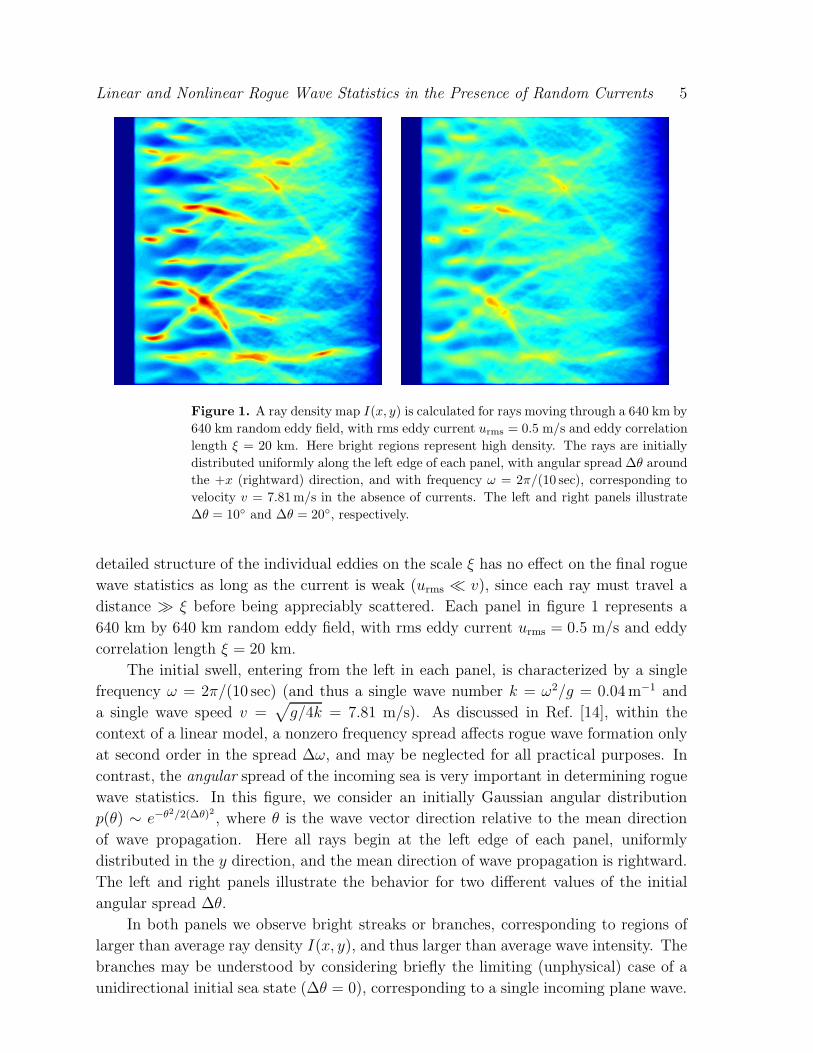
Figure 1. A ray density map I(x, y) is calculated for rays moving through a 640 km by

640 km random eddy field, with rms eddy current urms = 0.5 m/s and eddy correlation

length ξ = 20 km. Here bright regions represent high density. The rays are initially

distributed uniformly along the left edge of each panel, with angular spread ∆θ around

the +x (rightward) direction, and with frequency ω = 2π/(10 sec), corresponding to

velocity v = 7.81m/s in the absence of currents. The left and right panels illustrate

∆θ = 10◦ and ∆θ = 20◦, respectively.

detailed structure of the individual eddies on the scale ξ has no effect on the final rogue

wave statistics as long as the current is weak (urms ≪ v), since each ray must travel a

distance ≫ ξ before being appreciably scattered. Each panel in figure 1 represents a

640 km by 640 km random eddy field, with rms eddy current urms = 0.5 m/s and eddy

correlation length ξ = 20 km.

The initial swell, entering from the left in each panel, is characterized by a single

frequency ω = 2π/(10 sec) (and thus a single wave number k = ω2/g = 0.04m−1 and

a single wave speed v =√

g/4k = 7.81 m/s). As discussed in Ref. [14], within the

context of a linear model, a nonzero frequency spread affects rogue wave formation only

at second order in the spread ∆ω, and may be neglected for all practical purposes. In

contrast, the angular spread of the incoming sea is very important in determining rogue

wave statistics. In this figure, we consider an initially Gaussian angular distribution

p(θ) ∼ e−θ2/2(∆θ)2 , where θ is the wave vector direction relative to the mean direction

of wave propagation. Here all rays begin at the left edge of each panel, uniformly

distributed in the y direction, and the mean direction of wave propagation is rightward.

The left and right panels illustrate the behavior for two different values of the initial

angular spread ∆θ.

In both panels we observe bright streaks or branches, corresponding to regions of

larger than average ray density I(x, y), and thus larger than average wave intensity. The

branches may be understood by considering briefly the limiting (unphysical) case of a

unidirectional initial sea state (∆θ = 0), corresponding to a single incoming plane wave.


In the ray picture, and in the coordinates of figure 1, the initial conditions are in this

limit characterized by a one-dimensional phase space manifold (x, y, kx, ky) = (0, y, k, 0),

where k is the fixed wave number, and y varies over all space. As this incoming plane

wave travels through the random current field, it undergoes small-angle scattering, with

scattering angle∼ urms/v after traveling one correlation length ξ in the forward direction.

Eventually, singularities appear that are characterized in the surface of section map

[y(0), ky(0)] → [y(x), ky(x)] by δy(x)/δy(0) = 0, i.e., by local focusing of the manifold

of initial conditions at a point (x, y).

The currents leading to such a focusing singularity may be thought of as forming

a ‘bad lens.’ Whereas a lens without aberration focuses all parallel incoming rays to

one point, a bad lens only focuses at each point an infinitesimal neighborhood of nearby

rays, so that different neighborhoods get focused at different places as the phase-space

manifold evolves forward in x, resulting in lines, or branches, of singularities. The typical

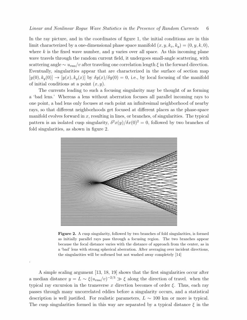
pattern is an isolated cusp singularity, δ2x(y)/δx(0)2 = 0, followed by two branches of

fold singularities, as shown in figure 2.

Figure 2. A cusp singularity, followed by two branches of fold singularities, is formed

as initially parallel rays pass through a focusing region. The two branches appear

because the focal distance varies with the distance of approach from the center, as in

a ‘bad’ lens with strong spherical aberration. After averaging over incident directions,

the singularities will be softened but not washed away completely [14]

.

A simple scaling argument [13, 18, 19] shows that the first singularities occur after

a median distance y = L ∼ ξ(urms/v)−2/3 ≫ ξ along the direction of travel. when the

typical ray excursion in the transverse x direction becomes of order ξ. Thus, each ray

passes through many uncorrelated eddies before a singularity occurs, and a statistical

description is well justified. For realistic parameters, L ∼ 100 km or more is typical.

The cusp singularities formed in this way are separated by a typical distance ξ in the


transverse direction, and thus the rms deflection angle by the time these singularities

appear scales as

δθ ∼ ξ/L ∼ (urms/v)2/3 . (5)

We note that the typical deflection angle δθ does not depend on the eddy size but

only on the velocity ratio urms/v: faster currents cause larger deflection. For the

input parameters used in figure 1, the median distance to the first singularity is

L = 7.5ξ = 150 km, and the rms deflection at the point of singularity is δθ = 18◦.

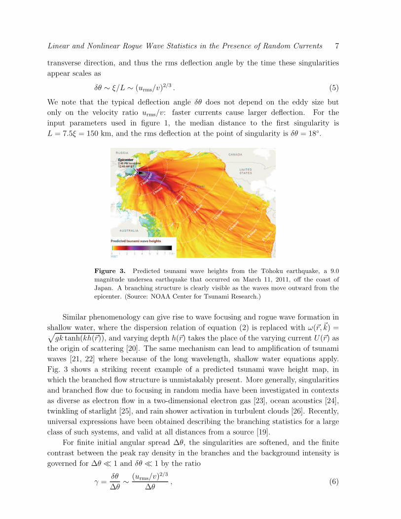
Figure 3. Predicted tsunami wave heights from the Tohoku earthquake, a 9.0

magnitude undersea earthquake that occurred on March 11, 2011, off the coast of

Japan. A branching structure is clearly visible as the waves move outward from the

epicenter. (Source: NOAA Center for Tsunami Research.)

Similar phenomenology can give rise to wave focusing and rogue wave formation in

shallow water, where the dispersion relation of equation (2) is replaced with ω(~r,~k) =√

gk tanh(kh(~r)), and varying depth h(~r) takes the place of the varying current U(~r) as

the origin of scattering [20]. The same mechanism can lead to amplification of tsunami

waves [21, 22] where because of the long wavelength, shallow water equations apply.

Fig. 3 shows a striking recent example of a predicted tsunami wave height map, in

which the branched flow structure is unmistakably present. More generally, singularities

and branched flow due to focusing in random media have been investigated in contexts

as diverse as electron flow in a two-dimensional electron gas [23], ocean acoustics [24],

twinkling of starlight [25], and rain shower activation in turbulent clouds [26]. Recently,

universal expressions have been obtained describing the branching statistics for a large

class of such systems, and valid at all distances from a source [19].

For finite initial angular spread ∆θ, the singularities are softened, and the finite

contrast between the peak ray density in the branches and the background intensity is

governed for ∆θ ≪ 1 and δθ ≪ 1 by the ratio

γ =δθ

∆θ∼ (urms/v)

2/3

∆θ, (6)


0

0.5

1

1.5

2

2.5

0 0.5 1 1.5 2 2.5 3

Pro

babi

lity

dist

ribut

ion

g(I

)

Ray intensity I

γ = 0.72γ = 1.20γ = 3.60

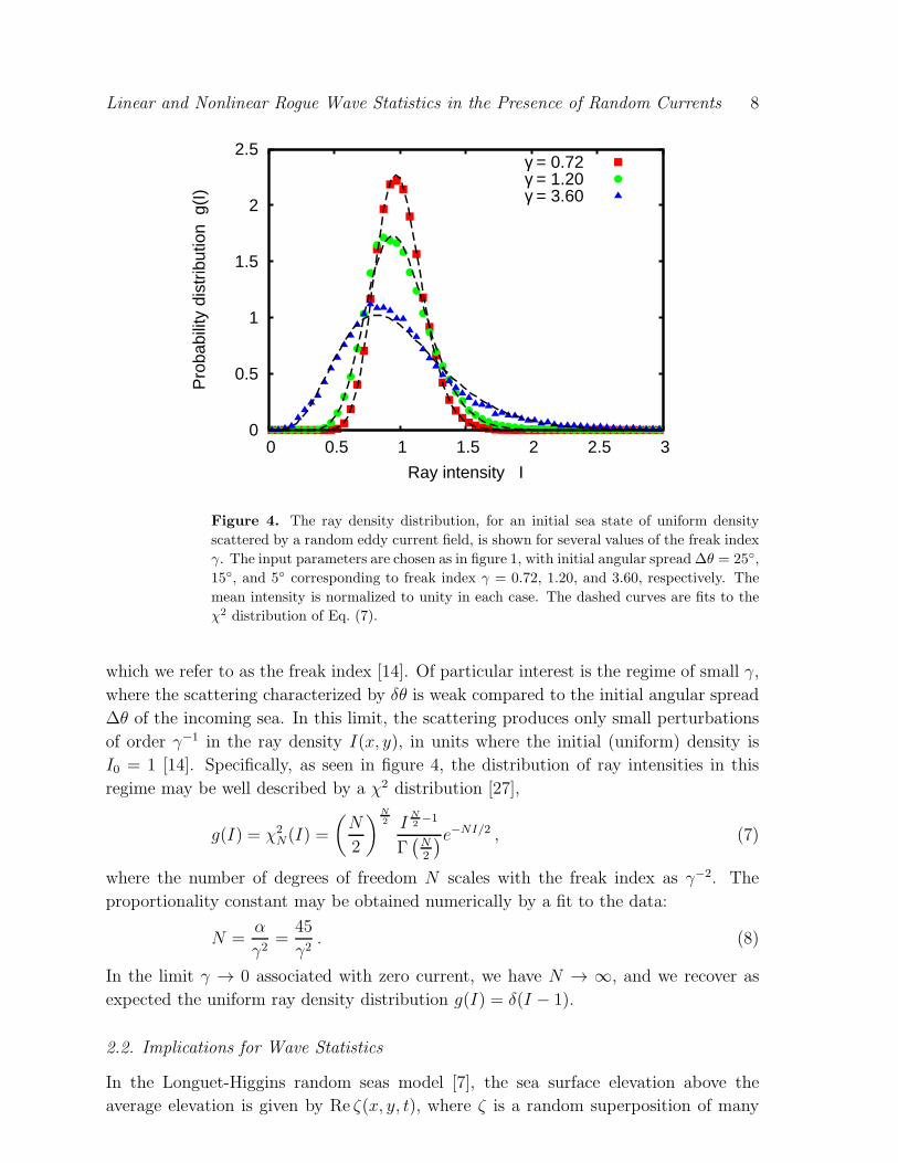
Figure 4. The ray density distribution, for an initial sea state of uniform density

scattered by a random eddy current field, is shown for several values of the freak index

γ. The input parameters are chosen as in figure 1, with initial angular spread ∆θ = 25◦,

15◦, and 5◦ corresponding to freak index γ = 0.72, 1.20, and 3.60, respectively. The

mean intensity is normalized to unity in each case. The dashed curves are fits to the

χ2 distribution of Eq. (7).

which we refer to as the freak index [14]. Of particular interest is the regime of small γ,

where the scattering characterized by δθ is weak compared to the initial angular spread

∆θ of the incoming sea. In this limit, the scattering produces only small perturbations

of order γ−1 in the ray density I(x, y), in units where the initial (uniform) density is

I0 = 1 [14]. Specifically, as seen in figure 4, the distribution of ray intensities in this

regime may be well described by a χ2 distribution [27],

g(I) = χ2N(I) =

(

N

2

)N

2 IN

2−1

Γ(

N2

)e−NI/2 , (7)

where the number of degrees of freedom N scales with the freak index as γ−2. The

proportionality constant may be obtained numerically by a fit to the data:

N =α

γ2=

45

γ2. (8)

In the limit γ → 0 associated with zero current, we have N → ∞, and we recover as

expected the uniform ray density distribution g(I) = δ(I − 1).

2.2. Implications for Wave Statistics

In the Longuet-Higgins random seas model [7], the sea surface elevation above the

average elevation is given by Re ζ(x, y, t), where ζ is a random superposition of many


plane waves with differing directions and frequencies. By the central limit theorem,

ζ is distributed as a complex Gaussian random variable with standard deviation σ.

Furthermore, for a narrow-banded spectrum (δω ≪ ω) the wave crest height H is equal

to the wave function amplitude |ζ |, and the probability of encountering a wave crest of

height H or larger is

PRayleigh(H) = e−H2/2σ2

. (9)

Due to an exact symmetry between crests and troughs in a linear wave model, a crest

height of H corresponds to a wave height (crest to trough) of 2H . Conventionally, a

rogue wave is defined as 2H ≥ 2.2 SWH, where the significant wave height SWH is

the average of the largest one third of wave heights in a time series, or approximately

SWH ≈ 4.0σ. Thus the condition for a rogue wave is H ≥ 4.4σ, and the random

seas model predicts such waves to occur with probability PRayleigh(4.4σ) = 6.3 · 10−5.

Similarly, extreme rogue waves may be defined by the condition 2H ≥ 3 SWH or

H ≥ 6.0σ, and these are predicted to occur with probability PRayleigh(6.0σ) = 1.5 · 10−8

within the random seas model. As discussed in section 1, the random seas model

greatly underestimates the occurrence probability of extreme waves, when compared

with observational data [2].

What are the implications of scattering by currents, as discussed in section 2.1,

on the wave height statistics? Within the regime of validity of the ray approximation,

we have at any spatial point (x, y) correspondence between the ray density I(x, y) and

the wave intensity H2 = |ζ(x, y, t)|2, averaged over time. Thus, in contrast with the

original Longuet-Higgins model, the time-averaged wave intensity is not uniform over

all space but instead exhibits “hot spots” and “cold spots” associated with focusing

and defocusing in the corresponding ray equations. At each point in space (assuming of

course that the currents are stationary), the central limit theorem and thus the Rayleigh

distribution still apply, and we have

P(x,y)(H) = e−H2/2σ2I(x,y) , (10)

where I(x, y) is the local ray density, normalized so that the spatial average is unity, and

σ2 is the variance of the surface elevation in the incoming sea state, before scattering

by currents. This is the situation a ship experiences at a given position.

Now averaging over space, or over an ensemble of random eddy fields with a given

rms current speed, we obtain a total cumulative height distribution

Ptotal(H) =

∫ ∞

0

dI g(I) e−H2/2σ2I . (11)

In equation (11), the full cumulative distribution of wave heights for a given sea state has

been expressed as a convolution of two factors: (i) the local density distribution g(I),

which can be extracted from the ray dynamics, and (ii) the universal Longuet-Higgins

distribution of wave heights for a given local density. Similar decompositions of chaotic

wave function statistics into non-universal and universal components have found broad

applicability in quantum chaos, including for example in the theory of scars [28, 29]. In


the context of rogue waves, a similar approach was adopted by Regev et al. to study wave

statistics in a one-dimensional inhomogeneous sea, where the inhomogeneity arises from

the interaction of an initially homogeneous sea with a (deterministic) long swell [30].

Using the previously obtained ray density distribution in the presence of currents,

equation (7), we obtain the K-distribution [31]

Ptotal(H) = 2

(√NH/2σ

)N

2

Γ(N/2)KN/2

(√NHσ

)

, (12)

where Kn(y) is a modified Bessel function.

Defining the dimensionless variable x = 2H/SWH ≈ 2H/(4σ), so that a rogue wave

is given by x = 2.2 and an extreme rogue wave by x = 3.0, we find the probability of a

wave height exceeding x significant wave heights:

Ptotal(x) = 2

(√Nx

)N

2

Γ(N/2)KN/2

(

2√Nx

)

, (13)

to be compared with the random seas prediction

PRayleigh(x) = e−2x2

(14)

in the same dimensionless units. We recall that N in equation (12) or (13) is a function

of the freak index γ, as given by equation (8).

To examine the predicted enhancement in the probability of rogue wave formation,

as compared with random seas model (9), we may consider two limiting cases. Keeping

the wave height of interest fixed, and taking the limit γ → 0, i.e. N → ∞, we obtain

the perturbative result

Pperturb(x) =

[

1 +4

N(x4 − x2)

]

PRayleigh(x) (15)

=

[

1 +4γ2

b(x4 − x2)

]

PRayleigh(x) , (16)

valid for x4 ≪ N , or equivalently x2γ ≪ 1. Thus, in the limit of small freak index, the

distribution reduces, as expected, to the prediction of the random seas model. Analogous

perturbative corrections appear for quantum wave function intensity distributions in the

presence of weak disorder or weak scarring by periodic orbits [32, 33].

Much more dramatic enhancement is observed if we consider the tail of the intensity

distribution (x→ ∞) for a given set of sea conditions (fixed γ orN). Then for x≫ N3/2,

or equivalently xγ3 ≫ 1, we obtain the asymptotic form

Pasymptotic(x) =√π

(√Nx

)N−1

2

Γ(N/2)e−2x

√N

=√π

(√Nx

)N−1

2

Γ(N/2)e2x(x−

√N)PRayleigh(x) , (17)


i.e., the probability enhancement over the random seas model is manifestly super-

exponential in the wave height x.

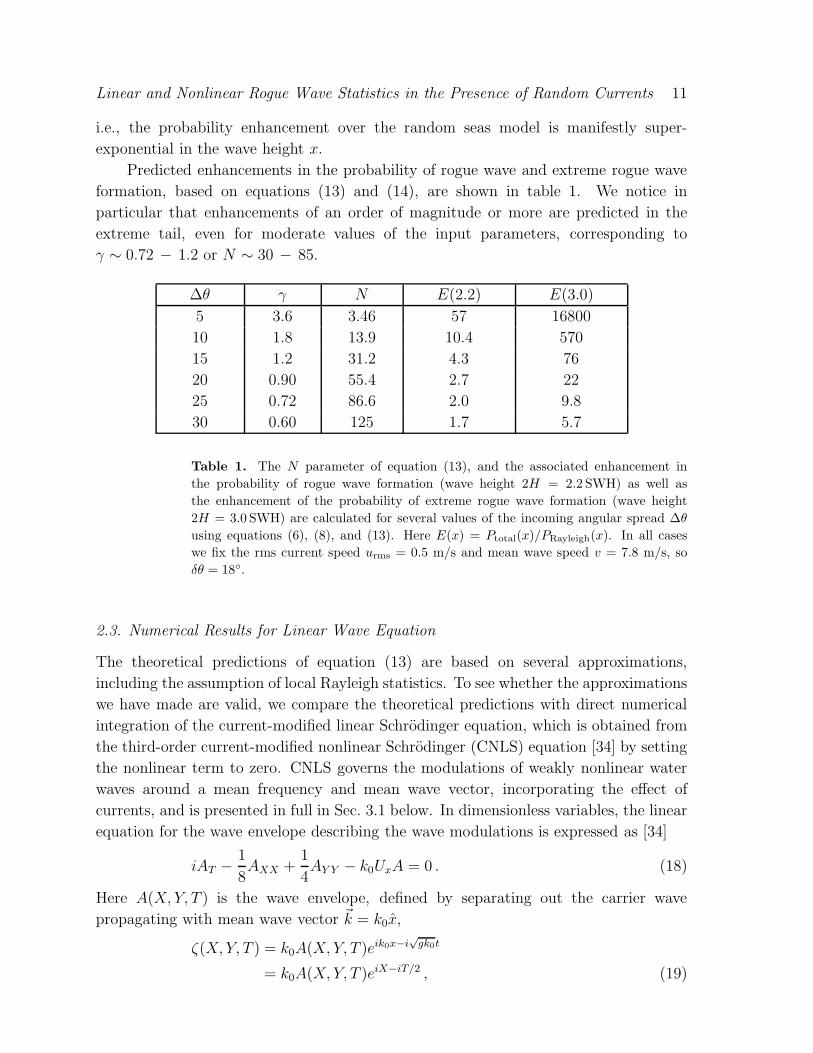
Predicted enhancements in the probability of rogue wave and extreme rogue wave

formation, based on equations (13) and (14), are shown in table 1. We notice in

particular that enhancements of an order of magnitude or more are predicted in the

extreme tail, even for moderate values of the input parameters, corresponding to

γ ∼ 0.72 − 1.2 or N ∼ 30 − 85.

∆θ γ N E(2.2) E(3.0)

5 3.6 3.46 57 16800

10 1.8 13.9 10.4 570

15 1.2 31.2 4.3 76

20 0.90 55.4 2.7 22

25 0.72 86.6 2.0 9.8

30 0.60 125 1.7 5.7

Table 1. The N parameter of equation (13), and the associated enhancement in

the probability of rogue wave formation (wave height 2H = 2.2 SWH) as well as

the enhancement of the probability of extreme rogue wave formation (wave height

2H = 3.0 SWH) are calculated for several values of the incoming angular spread ∆θ

using equations (6), (8), and (13). Here E(x) = Ptotal(x)/PRayleigh(x). In all cases

we fix the rms current speed urms = 0.5 m/s and mean wave speed v = 7.8 m/s, so

δθ = 18◦.

2.3. Numerical Results for Linear Wave Equation

The theoretical predictions of equation (13) are based on several approximations,

including the assumption of local Rayleigh statistics. To see whether the approximations

we have made are valid, we compare the theoretical predictions with direct numerical

integration of the current-modified linear Schrodinger equation, which is obtained from

the third-order current-modified nonlinear Schrodinger (CNLS) equation [34] by setting

the nonlinear term to zero. CNLS governs the modulations of weakly nonlinear water

waves around a mean frequency and mean wave vector, incorporating the effect of

currents, and is presented in full in Sec. 3.1 below. In dimensionless variables, the linear

equation for the wave envelope describing the wave modulations is expressed as [34]

iAT − 1

8AXX +

1

4AY Y − k0UxA = 0 . (18)

Here A(X, Y, T ) is the wave envelope, defined by separating out the carrier wave

propagating with mean wave vector ~k = k0x,

ζ(X, Y, T ) = k0A(X, Y, T )eik0x−i

√gk0t

= k0A(X, Y, T )eiX−iT/2 , (19)


and

(X, Y, T ) = (k0x−1

2

√

gkt, k0y,√

gk0t) (20)

are dimensionless space and time coordinates. We also note that Eq. (18) may be

obtained directly from the dispersion relation (2), by expanding ω and ~k around ω0 and

k0x, respectively.

10-8

10-7

10-6

10-5

10-4

10-3

10-2

10-1

100

0 0.5 1 1.5 2 2.5 3 3.5

Cum

ulat

ive

Pro

babi

lity

Wave Height / SWH

Numerical DataK Distribution

Rayleigh

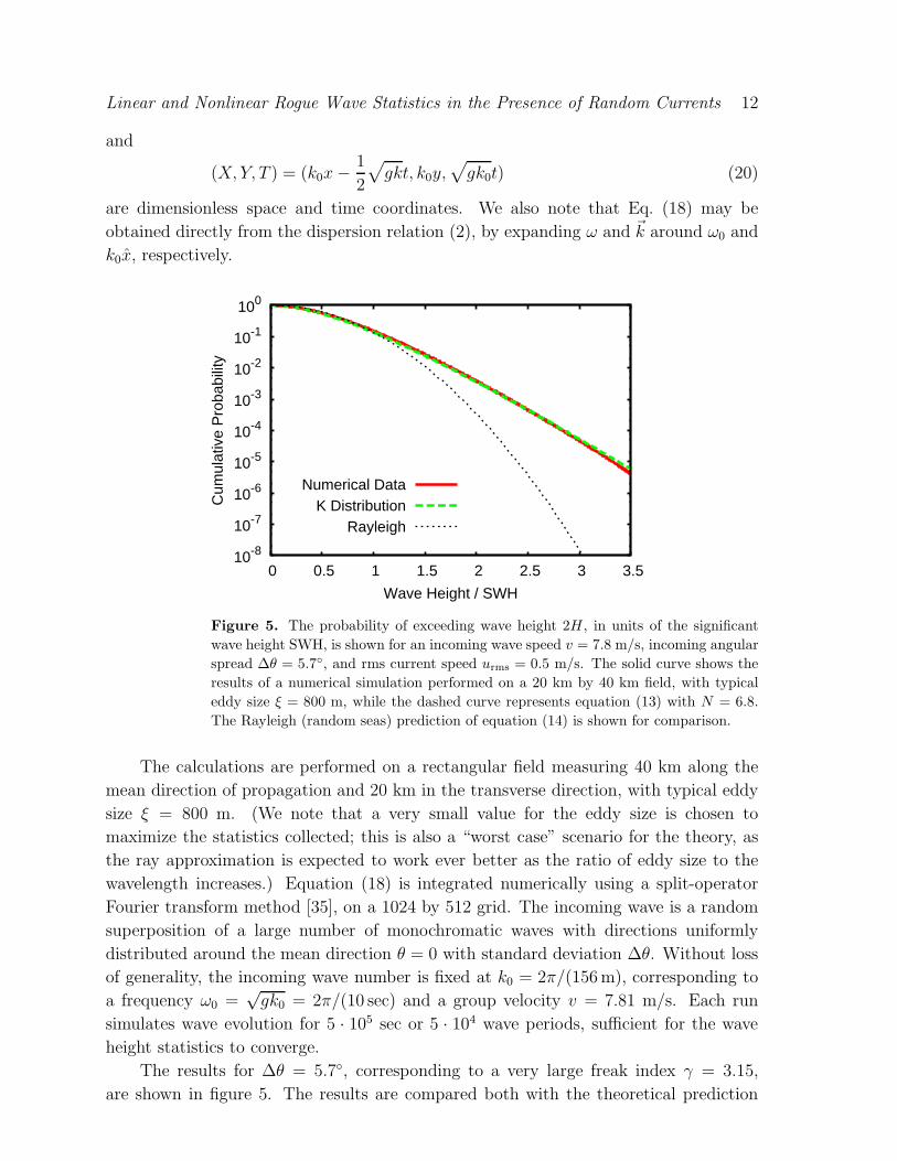
Figure 5. The probability of exceeding wave height 2H , in units of the significant

wave height SWH, is shown for an incoming wave speed v = 7.8 m/s, incoming angular

spread ∆θ = 5.7◦, and rms current speed urms = 0.5 m/s. The solid curve shows the

results of a numerical simulation performed on a 20 km by 40 km field, with typical

eddy size ξ = 800 m, while the dashed curve represents equation (13) with N = 6.8.

The Rayleigh (random seas) prediction of equation (14) is shown for comparison.

The calculations are performed on a rectangular field measuring 40 km along the

mean direction of propagation and 20 km in the transverse direction, with typical eddy

size ξ = 800 m. (We note that a very small value for the eddy size is chosen to

maximize the statistics collected; this is also a “worst case” scenario for the theory, as

the ray approximation is expected to work ever better as the ratio of eddy size to the

wavelength increases.) Equation (18) is integrated numerically using a split-operator

Fourier transform method [35], on a 1024 by 512 grid. The incoming wave is a random

superposition of a large number of monochromatic waves with directions uniformly

distributed around the mean direction θ = 0 with standard deviation ∆θ. Without loss

of generality, the incoming wave number is fixed at k0 = 2π/(156m), corresponding to

a frequency ω0 =√gk0 = 2π/(10 sec) and a group velocity v = 7.81 m/s. Each run

simulates wave evolution for 5 · 105 sec or 5 · 104 wave periods, sufficient for the wave

height statistics to converge.

The results for ∆θ = 5.7◦, corresponding to a very large freak index γ = 3.15,

are shown in figure 5. The results are compared both with the theoretical prediction


of equation (13) (here N = 6.8) and with the baseline Rayleigh distribution of

equation (14). This is an extreme scenario, in which the occurrence probability of

extreme rogue waves (3 times the significant wave height) is enhanced by more than three

orders of magnitude. Even better agreement with the theoretical model of equation (13)

obtains for more moderate values of γ, corresponding to larger N .

5

10

20

50

100

0.5 1 1.5 2 2.5 3

Deg

rees

of f

reed

om N

Freak index γ

urms = 0.2 m/surms = 0.3 m/surms = 0.4 m/surms = 0.5 m/s

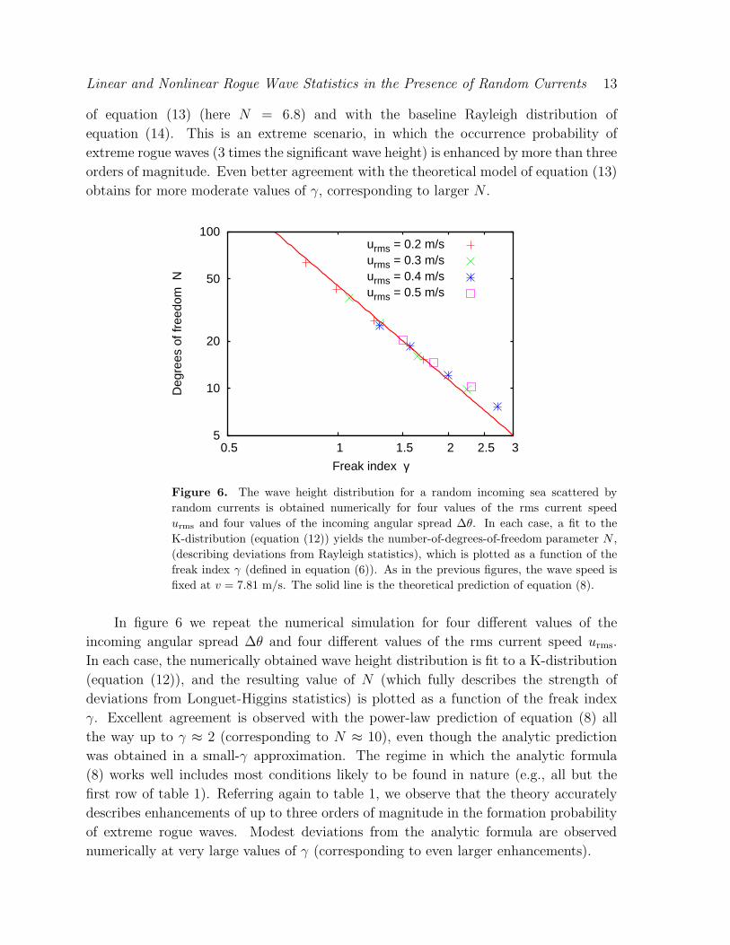
Figure 6. The wave height distribution for a random incoming sea scattered by

random currents is obtained numerically for four values of the rms current speed

urms and four values of the incoming angular spread ∆θ. In each case, a fit to the

K-distribution (equation (12)) yields the number-of-degrees-of-freedom parameter N ,

(describing deviations from Rayleigh statistics), which is plotted as a function of the

freak index γ (defined in equation (6)). As in the previous figures, the wave speed is

fixed at v = 7.81 m/s. The solid line is the theoretical prediction of equation (8).

In figure 6 we repeat the numerical simulation for four different values of the

incoming angular spread ∆θ and four different values of the rms current speed urms.

In each case, the numerically obtained wave height distribution is fit to a K-distribution

(equation (12)), and the resulting value of N (which fully describes the strength of

deviations from Longuet-Higgins statistics) is plotted as a function of the freak index

γ. Excellent agreement is observed with the power-law prediction of equation (8) all

the way up to γ ≈ 2 (corresponding to N ≈ 10), even though the analytic prediction

was obtained in a small-γ approximation. The regime in which the analytic formula

(8) works well includes most conditions likely to be found in nature (e.g., all but the

first row of table 1). Referring again to table 1, we observe that the theory accurately

describes enhancements of up to three orders of magnitude in the formation probability

of extreme rogue waves. Modest deviations from the analytic formula are observed

numerically at very large values of γ (corresponding to even larger enhancements).


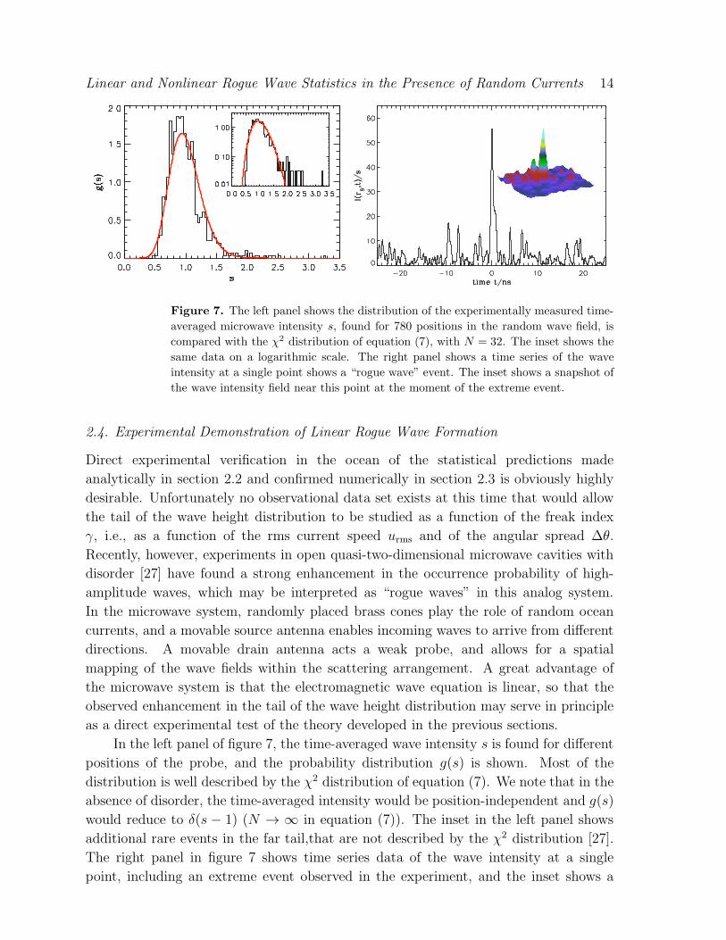
Figure 7. The left panel shows the distribution of the experimentally measured time-

averaged microwave intensity s, found for 780 positions in the random wave field, is

compared with the χ2 distribution of equation (7), with N = 32. The inset shows the

same data on a logarithmic scale. The right panel shows a time series of the wave

intensity at a single point shows a “rogue wave” event. The inset shows a snapshot of

the wave intensity field near this point at the moment of the extreme event.

2.4. Experimental Demonstration of Linear Rogue Wave Formation

Direct experimental verification in the ocean of the statistical predictions made

analytically in section 2.2 and confirmed numerically in section 2.3 is obviously highly

desirable. Unfortunately no observational data set exists at this time that would allow

the tail of the wave height distribution to be studied as a function of the freak index

γ, i.e., as a function of the rms current speed urms and of the angular spread ∆θ.

Recently, however, experiments in open quasi-two-dimensional microwave cavities with

disorder [27] have found a strong enhancement in the occurrence probability of high-

amplitude waves, which may be interpreted as “rogue waves” in this analog system.

In the microwave system, randomly placed brass cones play the role of random ocean

currents, and a movable source antenna enables incoming waves to arrive from different

directions. A movable drain antenna acts a weak probe, and allows for a spatial

mapping of the wave fields within the scattering arrangement. A great advantage of

the microwave system is that the electromagnetic wave equation is linear, so that the

observed enhancement in the tail of the wave height distribution may serve in principle

as a direct experimental test of the theory developed in the previous sections.

In the left panel of figure 7, the time-averaged wave intensity s is found for different

positions of the probe, and the probability distribution g(s) is shown. Most of the

distribution is well described by the χ2 distribution of equation (7). We note that in the

absence of disorder, the time-averaged intensity would be position-independent and g(s)

would reduce to δ(s − 1) (N → ∞ in equation (7)). The inset in the left panel shows

additional rare events in the far tail,that are not described by the χ2 distribution [27].

The right panel in figure 7 shows time series data of the wave intensity at a single

point, including an extreme event observed in the experiment, and the inset shows a


snapshot of the wave intensity in the region at the moment corresponding to this extreme

event. The event presented here has wave height 2H = 5.3 SWH, and events of this

magnitude of greater are observed with probability 1.3× 10−9 in the experiment, which

is an enhancement of 15 orders of magnitude compared to the Rayleigh distribution.

These results confirm that linear scattering is a sufficient mechanism for a large

enhancement in the tail of the wave height distribution, even when nonlinearity is

entirely absent from the physical system being studied.

3. Nonlinear Wave Model

We have already seen (e.g., in table 1) that under physically realistic sea conditions,

linear wave dynamics, with nonlinearity only in the corresponding ray equations,

are sufficient to enhance the incidence of extreme rogue waves by several orders of

magnitude. At the same time, the true equations for ocean wave evolution are certainly

nonlinear, and furthermore the nonlinear terms, which scale as powers of the wave height,

manifestly become ever more important in the tail of the wave height distribution. Thus,

a fully quantitative theory of rogue wave statistics must necessarily include nonlinear

effects, which we address in the following.

3.1. Nonlinear Schrodinger Equation

The original Nonlinear Schrodinger Equation (NLSE) for surface gravity waves in deep

water was derived by Zakharov using a spectral method [36], and is valid to third

order in the steepness ε = k0H , where H is the mean wave height. Subsequently,

the NLSE was extended to fourth order in ε by Dysthe [37] and then to higher order

in the bandwidth ∆ω/ω by Trulsen and Dysthe [38]. The Trulsen-Dysthe equations

include frequency downshifting [39], the experimentally observed reduction in average

frequency over time [40]; however the physics of frequency downshifting may not yet be

fully understood [41].

In our simulations we implement the current-modified O(ε4) NLSE, as derived by

Stocker and Peregrine in dimensionless form [34]:

iBT − 1

8(BXX − 2BY Y )−

1

2B|B|2 −BΦcX =

i

16(BXXX − 6BY Y X)

+ ΦXB +i

4B(BB∗

X − 6B∗BX) + i(1

2ΦcXT − ΦcZ)B − i∇hΦc · ∇hB ,(21)

where the the linear and third-order terms are collected on the left hand side of

equation (21). Here Φ, Φc, and B represent the mean flow, surface current, and

oscillatory parts, respectively of the velocity potential φ:

φ =

√

g

k30

[

Φ + Φc +1

2

(

Bek0z+iθ +B2e2(k0z+iθ) + c.c.

)

]

, (22)

where the second-harmonic term B2 is function of B and its derivatives, (X, Y, T )

are dimensionless space and time coordinates defined previously in equation (20), and


θ = k0x−√gk0t = X − T/2 is the phase. The surface elevation, which is the quantity

of interest for our purposes, is similarly expanded as

ζ = k0−1

[

ζ + ζc +1

2

(

Aiθ + A2e2iθ + A3e

3iθ + c.c.)

]

, (23)

where the expansion coefficients may be obtained from the velocity potential as

A = iB +1

2k0Bx +

i

8k20(Bxx − 2Byy) +

i

8B|B|2

A2 = − 1

2B2 +

i

k0BBx (24)

A3 = − 3i

8B3 .

***Here both B and A are of order ε, and proportion to ε. By changing the magnitude

of B or A in the incoming wave, we can set steepness to different value.

In the simulatin, for the simplicity, we works in the frame of reference moving

with the velocity v0 = (co + Uo, Vo), so Φ and Φc in equation (22) is zero. The

incoming wave is a random superposition of a large number of monochromatic waves

with different frequencies and propagating directions. Thus the initial wave could be

prepared analytically, as a linear summation of a large number of plain wave,

ψ(~r, t) =

N∑

1

φi =

N∑

1

Aiei ~ki·~r (25)

where ~ki is the random wave vector for each monochromatic wave. For our setup, the

wave vector can be expressed as

~k = (k0 + k′) · (cosθ′ ~x+ sinθ′ ~y) (26)

where k′ is a random variation in wave number follows a Gaussian distribution whose

half height width is ∆k, and θ′ is the angular spread which is a normal distribution with

stand deviation ∆θ.

In the following examples, equation (21) is integrated numerically with the current

set to zero, in order to investigate systematically and quantitatively the effect of

nonlinear focusing. In nature, the interplay between linear and nonlinear mechanisms is

also of great interest, and may give rise to even stronger enhancement in the probability

of rogue wave occurrence than either effect individually, as demonstrated below in

section 4 (see also [42, 43]).

3.2. Height Distribution

As in the linear case, the split-operator Fourier transform method is used to integrate

equation (21) numerically. The rectangular field measuring 20 km along the mean

direction of propagation and 10 km in the transverse direction is discretized using a 1024

by 512 grid. The incoming state is a random superposition of plane waves with wave

numbers normally distributed around k0 with standard deviation ∆k, and directions

uniformly distributed around the mean direction θ = 0 with standard deviation ∆θ.


Without loss of generality we fix the mean incoming wave number at k0 = 2π/(156m),

as in section 2. The steepness k0H is adjusted by varying the mean height H of the

incoming sea. Each run simulates wave evolution for 4 · 106 sec or 4 · 105 wave periods.

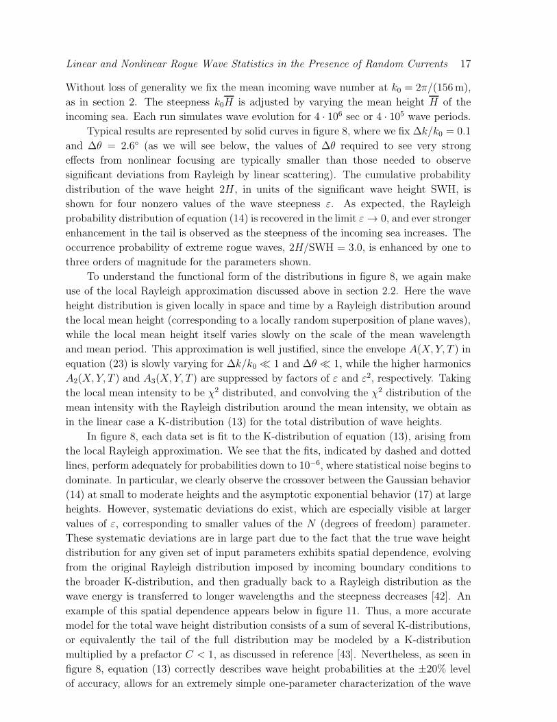
Typical results are represented by solid curves in figure 8, where we fix ∆k/k0 = 0.1

and ∆θ = 2.6◦ (as we will see below, the values of ∆θ required to see very strong

effects from nonlinear focusing are typically smaller than those needed to observe

significant deviations from Rayleigh by linear scattering). The cumulative probability

distribution of the wave height 2H , in units of the significant wave height SWH, is

shown for four nonzero values of the wave steepness ε. As expected, the Rayleigh

probability distribution of equation (14) is recovered in the limit ε→ 0, and ever stronger

enhancement in the tail is observed as the steepness of the incoming sea increases. The

occurrence probability of extreme rogue waves, 2H/SWH = 3.0, is enhanced by one to

three orders of magnitude for the parameters shown.

To understand the functional form of the distributions in figure 8, we again make

use of the local Rayleigh approximation discussed above in section 2.2. Here the wave

height distribution is given locally in space and time by a Rayleigh distribution around

the local mean height (corresponding to a locally random superposition of plane waves),

while the local mean height itself varies slowly on the scale of the mean wavelength

and mean period. This approximation is well justified, since the envelope A(X, Y, T ) in

equation (23) is slowly varying for ∆k/k0 ≪ 1 and ∆θ ≪ 1, while the higher harmonics

A2(X, Y, T ) and A3(X, Y, T ) are suppressed by factors of ε and ε2, respectively. Taking

the local mean intensity to be χ2 distributed, and convolving the χ2 distribution of the

mean intensity with the Rayleigh distribution around the mean intensity, we obtain as

in the linear case a K-distribution (13) for the total distribution of wave heights.

In figure 8, each data set is fit to the K-distribution of equation (13), arising from

the local Rayleigh approximation. We see that the fits, indicated by dashed and dotted

lines, perform adequately for probabilities down to 10−6, where statistical noise begins to

dominate. In particular, we clearly observe the crossover between the Gaussian behavior

(14) at small to moderate heights and the asymptotic exponential behavior (17) at large

heights. However, systematic deviations do exist, which are especially visible at larger

values of ε, corresponding to smaller values of the N (degrees of freedom) parameter.

These systematic deviations are in large part due to the fact that the true wave height

distribution for any given set of input parameters exhibits spatial dependence, evolving

from the original Rayleigh distribution imposed by incoming boundary conditions to

the broader K-distribution, and then gradually back to a Rayleigh distribution as the

wave energy is transferred to longer wavelengths and the steepness decreases [42]. An

example of this spatial dependence appears below in figure 11. Thus, a more accurate

model for the total wave height distribution consists of a sum of several K-distributions,

or equivalently the tail of the full distribution may be modeled by a K-distribution

multiplied by a prefactor C < 1, as discussed in reference [43]. Nevertheless, as seen in

figure 8, equation (13) correctly describes wave height probabilities at the ±20% level

of accuracy, allows for an extremely simple one-parameter characterization of the wave


0 1 2 3 410-7

10-5

0.001

0.1

Wave Height�SWH

Cum

ulat

ive

Pro

babi

lity

¶=0.042

¶=0.026

¶=0.019

¶=0

Figure 8. The distribution of wave heights, in units of the significant wave height, is

calculated for three nonzero values of the steepness ε (upper three solid curves), and

compared with the random seas model of equation (14) (lowest solid curve). In each

case, the dashed or dotted curve is a best fit to the K-distribution of equation (13).

Here the we fix the angular spread ∆θ = 2.6◦ and wave number spread ∆k/k0 = 0.1

of the incoming sea.

height distribution, and facilitates easy comparison between the effects of linear and

nonlinear focusing.

3.3. Scaling with Input Parameters

Given the single-parameter approximation of equation (13), it is sufficient to explore

the dependence of the parameter N on the input variables describing the incoming sea,

specifically the initial angular spread ∆θ, the initial wave number spread ∆k/k0, and

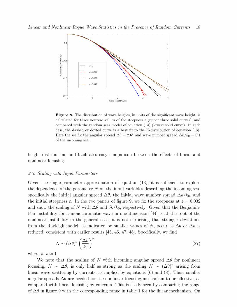
the initial steepness ε. In the two panels of figure 9, we fix the steepness at ε = 0.032

and show the scaling of N with ∆θ and δk/k0, respectively. Given that the Benjamin-

Feir instability for a monochromatic wave in one dimension [44] is at the root of the

nonlinear instability in the general case, it is not surprising that stronger deviations

from the Rayleigh model, as indicated by smaller values of N , occur as ∆θ or ∆k is

reduced, consistent with earlier results [45, 46, 47, 48]. Specifically, we find

N ∼ (∆θ)a(

∆k

k0

)b

(27)

where a, b ≈ 1.

We note that the scaling of N with incoming angular spread ∆θ for nonlinear

focusing, N ∼ ∆θ, is only half as strong as the scaling N ∼ (∆θ)2 arising from

linear wave scattering by currents, as implied by equations (6) and (8). Thus, smaller

angular spreads ∆θ are needed for the nonlinear focusing mechanism to be effective, as

compared with linear focusing by currents. This is easily seen by comparing the range

of ∆θ in figure 9 with the corresponding range in table 1 for the linear mechanism. On


ææ

æ

æ

æ

æ ææ

æ

æ

æææææ

æ

ææ

¢

¢

¢

¢

¢

¢¢

¢

¢¢

¢ ¢

¢ ¢

¢ ¢

¢ ¢

à

à

à àà

à

àà

à

à

à àà

àà à

àà

ìì ì

ì ì

ìì

ìì

ìì

ì ì

ì ì

ì

ì

ì

æ

æ

æ

æ

æ

æ

æ

æ

æ

æ

æ

æ

æ

æ

æ

æ

æ

æ

æ

æ

æ

æ

æ

æ

æ

æ

æ

æ

æ

æ

æ

æ

æ

æ

æ

æ

æ

æ

æ

æ

æ

æ

æ

æ

æ

æ

æ

æ

æ

æ

æ

æ

æ

æ

æ

æ

æ

æ

æ

æ

æ

æ

æ

æ

æ

æ

æ

æ

æ

æ

æ

æ

æ

æ

æ

æ

æ

æ

æ

æ

æ

æ

æ

æ

æ

æ

æ

æ

æ

æ

æ

æ

æ

æ

æ

æ

æ

æ

æ

æ

æ

æ

æ

æ

æ

æ

æ

æ

æ

æ

æ

æ

æ

æ

æ

æ

æ

æ

æ

æ

æ

æ

æ

æ

æ

æ

æ

æ

æ

æ

æ

æ

æ

æ

æ

æ

æ

æ

æ

æ

æ

æ

æ

æ

æ

æ

æ

æ

æ

æ

æ

æ

æ

æ

æ

æ

æ

æ

æ

æ

æ

æ

æ

æ

æ

æ

æ

æ

æ

æ

æ

æ

æ

æ

æ

æ

æ

æ

æ

æ

æ

æ

æ

æ

æ

æ

æ

æ

æ

æ

æ

æ

æ

æ

æ

æ

æ

æ

æ

æ

æ

æ

æ

æ

æ

æ

æ

æ

æ

æ

æ

æ

æ

æ

æ

æ

æ

æ

æ

æ

æ

æ

æ

æ

æ

æ

æ

æ

æ

æ

æ

æ

æ

æ

æ

æ

æ

æ

æ

æ

æ

æ

æ

æ

æ

æ

æ

æ

æ

æ

æ

æ

æ

æ

æ

æ

æ

æ

æ

æ

æ

æ

æ

æ

æ

æ

æ

æ

æ

æ

æ

æ

æ

æ

æ

æ

æ

æ

æ

æ

æ

æ

æ

æ

æ

æ

æ

æ

æ

æ

æ

æ

æ

æ

æ

æ

æ

æ

æ

æ

æ

æ

æ

æ

æ

æ

æ

æ

æ æ æ æ æ æ æ æ æ æ æ æ æ æ æ æ æ æ æ æ æ æ æ æ æ æ æ æ æ æ æ æ æ æ æ æ æ æ æ æ æ æ æ æ æ æ æ æ æ æ æ æ æ æ æ æ æ æ æ æ æ æ æ æ æ æ æ æ æ æ æ æ æ æ æ æ æ æ æ æ æ æ æ æ æ æ æ æ æ æ æ æ æ æ æ æ æ æ æ æ æ æ æ æ æ æ æ æ æ æ æ æ æ æ æ æ æ æ æ æ æ æ æ æ æ æ æ æ æ æ æ æ æ æ æ æ æ æ æ æ æ æ æ æ æ æ æ æ æ æ æ æ æ æ æ æ æ æ æ æ æ æ æ æ æ æ æ æ æ æ æ æ æ æ æ æ æ æ æ æ æ æ æ æ æ æ æ æ æ æ æ æ æ æ æ æ æ æ æ æ æ æ æ æ æ æ æ æ æ æ æ æ æ æ æ æ æ æ æ æ æ æ æ æ æ æ æ æ æ æ æ æ æ æ æ æ æ æ æ æ æ æ æ æ æ æ æ æ æ æ æ æ æ æ æ æ æ æ æ æ æ æ æ æ æ æ æ æ æ æ æ æ æ æ æ æ æ æ æ æ æ æ æ æ æ æ æ æ æ æ æ æ æ æ æ æ æ æ æ æ æ æ æ æ æ æ æ æ æ æ æ æ æ æ æ æ æ æ æ æ æ æ æ æ æ æ æ æ æ æ æ æ æ æ æ æ æ æ æ æ æ æ æ æ æ æ æ æ æ æ æ æ æ æ æ æ æ æ æ æ æ æ æ æ æ æ æ æ æ æ æ æ æ æ æ æ æ æ æ æ æ æ æ æ æ æ æ æ æ æ æ æ æ æ æ æ æ æ æ æ æ æ æ æ æ æ æ æ æ æ æ æ æ æ æ æ æ æ æ æ æ æ æ

1.0 5.02.0 3.01.5 7.0

10

100

50

20

30

15

70

ΘH°L

N

æ fit Dk�ko=0.15

ì Dk�ko=0.20

à Dk�ko=0.15

¢ Dk�ko=0.1

æ Dk�ko=0.08

ææ

æ

æ

æ æ

æ

ææ

æ

æ

æ

ææ æ

ææ

æææ

¢¢ ¢ ¢

¢ ¢

¢

¢

¢

¢ ¢ ¢

¢ ¢ ¢¢ ¢

¢

¢

¢

à à

à à

àà

à à

àà à à

à

à

à

à

à

à àà

ì

ì

ìì

ì ì

ì

ì

ì

ì

ì

ìì

ìì

ì

ì ì

ìì

æ

æ

æ

æ

æ

æ

æ

æ

æ

æ

æ

æ

æ

æ

æ

æ

æ

æ

æ

æ

æ

æ

0.10 0.200.15

10

50

20

30

15

70

Dk �ko

N

æ fit Θ=2.6°

ì Θ=1.0°

à Θ=2.6°

¢ Θ=3.6°

æ Θ=5.2°

Figure 9. The best-fit N value (equation (13)) describing the wave height probability

distribution is shown as a function of the initial angular spread ∆θ and initial wave

number spread ∆k/k0 of the incoming sea. The steepness is fixed at ε = 0.032. The

left panel shows the scaling of N with ∆θ, with the line showing the best-fit scaling

N ∼ (∆θ)1.04 for ∆k/k0 = 0.15. The right panel shows the scaling of N with ∆k/k0,

with the line showing the best-fit scaling N ∼ (∆k/k0)1.15 for ∆θ = 2.6◦.

the other hand, figure 9 and equation (27) both imply that the nonlinear mechanism

exhibits significant sensitivity to the spectral width ∆k/k0, consistent with previous

findings [6, 49, 50, 51, 52, 53]. This is to be contrasted with the linear mechanism of

rogue wave formation, which is insensitive to the spectral width at leading order in

∆k/k0 [14].

æææææ

ææ

ææ

æ

ææ

¢

¢

¢

¢¢

¢¢

¢

¢¢

¢

¢¢

¢¢ ¢

¢ ¢ ¢

à

à

à

àà

àà

àà

à

ààà

àà àààà

ì

ì ììì

ì

ììì ì

ììì

ìì

ìì

æ

æ

æ

æ

æ

æ

æ

æ

æ

æ

æ

æ

æ

æ

æ

æ

æ

æ

æ

æ

æ

æ

æ

æ

æ

æ

æ

æ

æ

æ

æ

æ

æ

æ

æ

æ

æ

æ

æ

æ

æ

æ

æ

æ

æ

æ

æ

æ

æ

æ

æ

æ

æ

æ

æ

æ

æ

æ

æ

æ

æ

æ

æ

æ

æ

æ

0.0500.020 0.0300.015 0.0701

2

5

10

20

50

100

SteepnessH¶L

N

æ fit Θ=3.6°ì Θ=5.2°à Θ=3.6°¢ Θ=2.6°æ Θ=1.0°

Angle

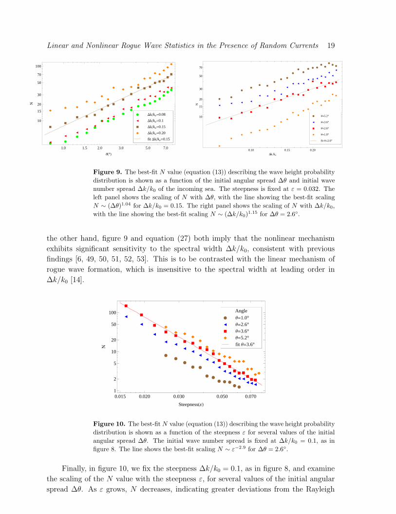
Figure 10. The best-fitN value (equation (13)) describing the wave height probability

distribution is shown as a function of the steepness ε for several values of the initial

angular spread ∆θ. The initial wave number spread is fixed at ∆k/k0 = 0.1, as in

figure 8. The line shows the best-fit scaling N ∼ ε−2.9 for ∆θ = 2.6◦.

Finally, in figure 10, we fix the steepness ∆k/k0 = 0.1, as in figure 8, and examine

the scaling of the N value with the steepness ε, for several values of the initial angular

spread ∆θ. As ε grows, N decreases, indicating greater deviations from the Rayleigh


distribution. Again, we observe good power-law scaling with the steepness in the range

of parameters considered here. We have

N ∼ εc (28)

where c ≈ −3. At larger values of the steepness (not shown), saturation occurs.

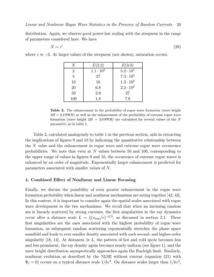
N E(2.2) E(3.0)

2 1.1 · 102 5.2 · 1045 37 7.3 · 10310 16 1.3 · 10320 6.8 2.2 · 10250 2.9 27

100 1.8 7.8

Table 2. The enhancement in the probability of rogue wave formation (wave height

2H = 2.2 SWH) as well as the enhancement of the probability of extreme rogue wave

formation (wave height 2H = 3.0 SWH) are calculated for several values of the N

parameter, as in table 1.

Table 2, calculated analogously to table 1 in the previous section, aids in extracting

the implications of figures 9 and 10 by indicating the quantitative relationship between

the N value and the enhancement in rogue wave and extreme rogue wave occurrence

probabilities. We note that even at N values between 50 and 100, corresponding to

the upper range of values in figures 9 and 10, the occurrence of extreme rogue waves is

enhanced by an order of magnitude. Exponentially larger enhancement is predicted for

parameters associated with smaller values of N .

4. Combined Effect of Nonlinear and Linear Focusing

Finally, we discuss the possibility of even greater enhancement in the rogue wave

formation probability when linear and nonlinear mechanisms are acting together [42, 43].

In this context, it is important to consider again the spatial scales associated with rogue

wave development in the two mechanisms. We recall that when an incoming random

sea is linearly scattered by strong currents, the first singularities in the ray dynamics

occur after a distance scale L ∼ ξ(urms/v)−2/3, as discussed in section 2.1. These

first singularities are the ones associated with the highest probability of rogue wave

formation, as subsequent random scattering exponentially stretches the phase space

manifold and leads to ever smaller density associated with each second- and higher-order

singularity [18, 14]. At distances ≫ L, the pattern of hot and cold spots becomes less

and less prominent, the ray density again becomes nearly uniform (see figure 1), and the

wave height distribution asymptotically approaches again the Rayleigh limit. Similarly,

nonlinear evolution as described by the NLSE without current (equation (21) with

Φc = 0) occurs on a typical distance scale 1/kε2. On distance scales larger than 1/kε2,


energy transfer from smaller to larger wavelengths (i.e., the frequency downshifting effect

mentioned previously in Sec. 3.1) results eventually in a decline in the steepness and

again an approach towards the limiting Rayleigh distribution [54, 10, 12].

0 2 4 6 8 10

1.

1.1

1.2

1.3

1.4

DistanceHkmL

H4 �

H4 R

aile

igh

¶=0.032,Urms=0.2 m�s

¶=0.032,Urms=0 m�s

¶=0, Urms=0.2 m�s

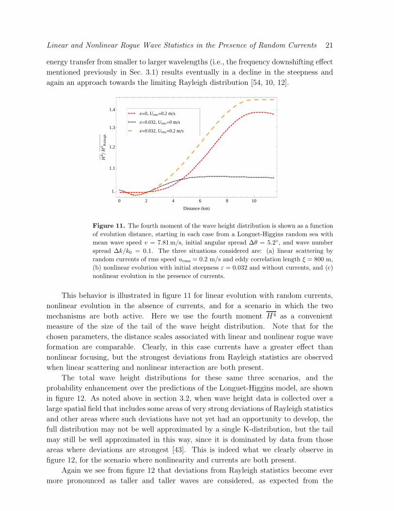
Figure 11. The fourth moment of the wave height distribution is shown as a function

of evolution distance, starting in each case from a Longuet-Higgins random sea with

mean wave speed v = 7.81m/s, initial angular spread ∆θ = 5.2◦, and wave number

spread ∆k/k0 = 0.1. The three situations considered are: (a) linear scattering by

random currents of rms speed urms = 0.2 m/s and eddy correlation length ξ = 800 m,

(b) nonlinear evolution with initial steepness ε = 0.032 and without currents, and (c)

nonlinear evolution in the presence of currents.

This behavior is illustrated in figure 11 for linear evolution with random currents,

nonlinear evolution in the absence of currents, and for a scenario in which the two

mechanisms are both active. Here we use the fourth moment H4 as a convenient

measure of the size of the tail of the wave height distribution. Note that for the

chosen parameters, the distance scales associated with linear and nonlinear rogue wave

formation are comparable. Clearly, in this case currents have a greater effect than

nonlinear focusing, but the strongest deviations from Rayleigh statistics are observed

when linear scattering and nonlinear interaction are both present.

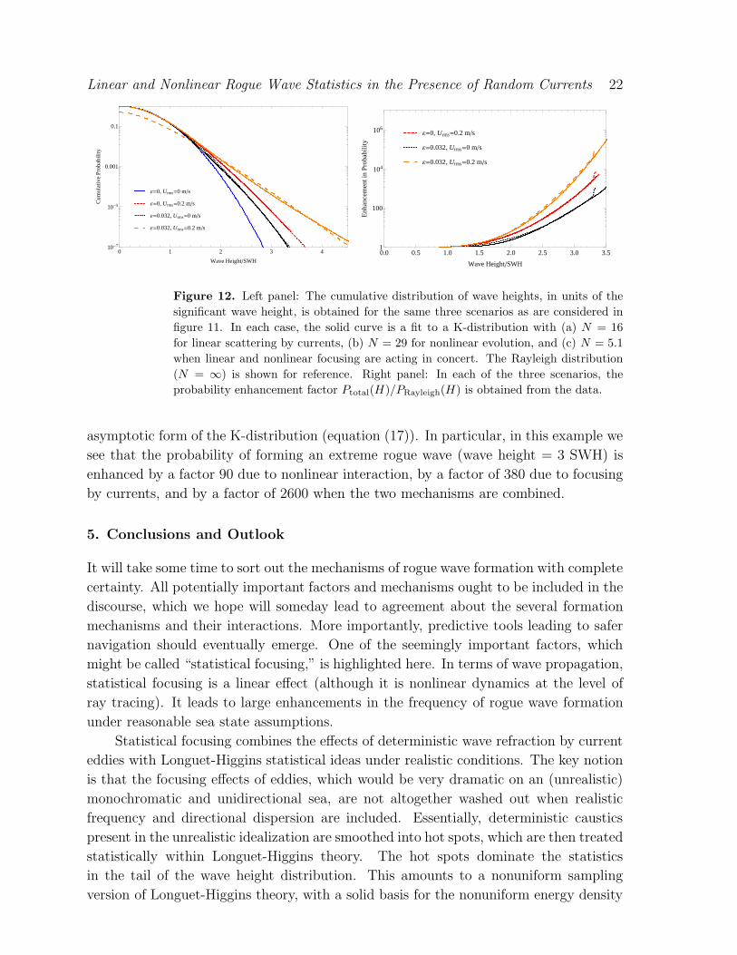
The total wave height distributions for these same three scenarios, and the

probability enhancement over the predictions of the Longuet-Higgins model, are shown

in figure 12. As noted above in section 3.2, when wave height data is collected over a

large spatial field that includes some areas of very strong deviations of Rayleigh statistics

and other areas where such deviations have not yet had an opportunity to develop, the

full distribution may not be well approximated by a single K-distribution, but the tail

may still be well approximated in this way, since it is dominated by data from those

areas where deviations are strongest [43]. This is indeed what we clearly observe in

figure 12, for the scenario where nonlinearity and currents are both present.

Again we see from figure 12 that deviations from Rayleigh statistics become ever

more pronounced as taller and taller waves are considered, as expected from the


0 1 2 3 410-7

10-5

0.001

0.1

Wave Height�SWH

Cum

ulat

ive

Pro

babi

lity

¶=0.032,Urms=0.2 m�s

¶=0.032,Urms=0 m�s

¶=0, Urms=0.2 m�s

¶=0, Urms=0 m�s

0.0 0.5 1.0 1.5 2.0 2.5 3.0 3.51

100

104

106

Wave Height�SWH

Enh

ance

men

tin

Pro

babi

lity

¶=0.032,Urms=0.2 m�s

¶=0.032,Urms=0 m�s

¶=0, Urms=0.2 m�s

Figure 12. Left panel: The cumulative distribution of wave heights, in units of the

significant wave height, is obtained for the same three scenarios as are considered in

figure 11. In each case, the solid curve is a fit to a K-distribution with (a) N = 16

for linear scattering by currents, (b) N = 29 for nonlinear evolution, and (c) N = 5.1

when linear and nonlinear focusing are acting in concert. The Rayleigh distribution

(N = ∞) is shown for reference. Right panel: In each of the three scenarios, the

probability enhancement factor Ptotal(H)/PRayleigh(H) is obtained from the data.

asymptotic form of the K-distribution (equation (17)). In particular, in this example we

see that the probability of forming an extreme rogue wave (wave height = 3 SWH) is

enhanced by a factor 90 due to nonlinear interaction, by a factor of 380 due to focusing

by currents, and by a factor of 2600 when the two mechanisms are combined.

5. Conclusions and Outlook

It will take some time to sort out the mechanisms of rogue wave formation with complete

certainty. All potentially important factors and mechanisms ought to be included in the

discourse, which we hope will someday lead to agreement about the several formation

mechanisms and their interactions. More importantly, predictive tools leading to safer

navigation should eventually emerge. One of the seemingly important factors, which

might be called “statistical focusing,” is highlighted here. In terms of wave propagation,

statistical focusing is a linear effect (although it is nonlinear dynamics at the level of

ray tracing). It leads to large enhancements in the frequency of rogue wave formation

under reasonable sea state assumptions.

Statistical focusing combines the effects of deterministic wave refraction by current

eddies with Longuet-Higgins statistical ideas under realistic conditions. The key notion

is that the focusing effects of eddies, which would be very dramatic on an (unrealistic)

monochromatic and unidirectional sea, are not altogether washed out when realistic

frequency and directional dispersion are included. Essentially, deterministic caustics

present in the unrealistic idealization are smoothed into hot spots, which are then treated

statistically within Longuet-Higgins theory. The hot spots dominate the statistics

in the tail of the wave height distribution. This amounts to a nonuniform sampling

version of Longuet-Higgins theory, with a solid basis for the nonuniform energy density


distributions used.

Since nonlinear effects are also important, we have examined them alone within

the popular fourth-order nonlinear Schrodinger equation (NLSE) approximation for

nonlinear wave evolution under realistic seaway conditions. Finally, we have investigated

the combined effect of nonlinear wave evolution and statistical focusing. We find

that strongest deviations from Rayleigh statistics are observed when linear scattering

(statistical focusing) and nonlinear interaction (NLSE) are both present. However,

for the parameters chosen here at least, the linear scattering due to eddies was more

important than the nonlinear effects, which require large steepness or a very narrow

range of propagation directions to become significant.

We have presented a measure closely related to the probability of rogue wave

formation, the freak index γ. This could conceivably become the basis for a probabilistic

forecast of rogue wave formation, in the spirit of rainfall forecasts.

There are at least three clear directions for future development of the work presented

here. First, both the computer simulations and the theory must be developed further to

explore fully and systematically the combined effects of nonlinear and linear focusing.

This will also involve investigating in depth the underlying mechanism through which

the formation of hot and cold spots is aided by nonlinear focusing. Secondly, a better

understanding is needed of the stability of the hot spot patterns under slow changes in

the current field or in the spectrum or directionality of the incoming sea. The strength

of what might be called scintillation or twinkling [25] in analogy with the case of light

traveling through the atmosphere will have important consequences for the predictive

power of the model. Thirdly, and most importantly, there is a clear need to compare the

model simulations with observations and experiments. Although comprehensive global

data are not available at this point, it may be possible to compare the results to local

observations where data are more readily available, e.g., in the North Sea.

Whatever the final word is on rogue wave formation (or final words, because there

may be more than one mechanism), it must involve a reallocation of energy from a larger

area to a smaller one. Waves cannot propagate and increase in height at no expense

to their neighbors: the energy has to come from somewhere, and the effect must be to

reduce the wave energy somewhere else. The focusing mechanism is clear in this respect:

hot spots form and cold spots do too, according to a ray tracing analysis, maintaining

energy balance [55].

Acknowledgments

This work was supported in part by the US NSF under Grant PHY-0545390.

References

[1] K. Trulsen and K. B. Dysthe, Proceedings of 21st Symposium on Naval Hydrodynamics, p. 550

(1997).


[2] H. Dankert, J. Horstmann, S. Lehner, and W. Rosenthal, IEEE Trans. Geosci. Remote Sens. 41,

1437 (2003).

[3] J. Schulz-Stellenfleth and S. Lehner, IEEE Trans. Geosci. Remote Sens. 42, 1149 (2004).

[4] K. B. Dysthe, H. E. Krogstad, and P. Muller, Annu. Rev. Fluid Mech. 40, 287 (2008).

[5] J. K. Mallory, Int. Hydrog. Rev. 51, 89 (1974).

[6] C. Kharif and E. Pelinovsky, Eur. F. Mech. 22, 603 (2003).

[7] M. S. Longuet-Higgins, Phil. Trans. R. Soc. London A 249, 321 (1957).

[8] G. Z. Forristall, J. Phys. Oceanogr. 30, 1931 (2000).

[9] M. Onorato, A. R. Osborne, M. Serio, L. Cavaleri, C. Brandini, and C. T. Stansberg, Phys. Rev.

E 70, 067302 (2004).

[10] M. Tanaka, J. Fluid. Mech. 444, 199 (2001).

[11] R. S. Gibson and P. H. Taylor, Appl. Ocean Res. 27, 142 (2005).

[12] R. S. Gibson and C. Swan, Proc. R. Soc. A 463, 21 (2007).

[13] B. S. White and B. Fornberg, J. Fluid. Mech. 355, 113 (1998).

[14] E. J. Heller, L. Kaplan, and A. Dahlen, J. Geophys. Res. 113, C09023 (2008).

[15] D. H. Peregrine, Adv. Appl. Mech. 16, 9 (1976); I. Lavrenov, Nat. Hazards 17, 117 (1998);

D. E. Irvine and D. G. Tilley, J. Geophys. Res. 93, 15389 (1988); M. L. Grundlingh, AVISO

Altimeter Newsl. 3 (1994).

[16] P. Jannsen and W. Alpers, Proc. SEASAR Workshop, 23-26 January 2006, ESA SP-613, Frascati,

Italy (2006).

[17] J. Schulz-Stellenfleth, T. Konig, and S. Lehner, J. Geophys. Res. 112, C03019 (2007).

[18] L. Kaplan, Phys. Rev. Lett. 89, 184103 (2002).

[19] J. J. Metzger, R. Fleischmann, and T. Geisel, Phys. Rev. Lett. 105, 020601 (2010).

[20] M. J. Tucker and E. G. Pitt, Waves in Ocean Engineering, Ocean Eng. Book Series, vol. 5, p. 521

(Elsevier, Amsterdam, 2001).

[21] M. V. Berry, New J. Phys. 7, 129 (2005); Proc. R. Soc. A 463, 3055 (2007).

[22] S. Y. Dobrokhotov, S. Y. Sekerzh-Zenkovich, B. Tirozzi, and T.Y. Tudorovskii, Doklady

Mathematics 74, 592 (2006).

[23] M. A. Topinka, B. J. LeRoy, R. M. Westervelt, S. E. J. Shaw, R. Fleischmann, E. J. Heller, K. D.

Maranowski, and A. C. Gossard, Nature (London) 410, 183 (2001); M. P. Jura, M. A. Topinka,

L. Urban, A. Yazdani, H. Shtrikman, L. N. Pfeiffer, K. W. West, and D. Goldhaber-Gordon,

Nat. Phys. 3, 841 (2007).

[24] M. Wolfson and S. Tomsovic, J. Acoust. Soc. Am. 109, 2693 (2001).

[25] M. V. Berry, J. Phys. A 10, 2061 (1977).

[26] M. Wilkinson, B. Mehlig, and V. Bezuglyy, Phys. Rev. Lett. 97, 048501 (2006).

[27] R. Hohmann, U. Kuhl, H.-J. Stockmann, L. Kaplan, and E. J. Heller, Phys. Rev. Lett. 104, 093901

(2010).

[28] L. Kaplan, Nonlinearity 12, R1 (1999); A. M. Smith and L. Kaplan, Phys. Rev. E 80, 035205(R)

(2009).

[29] A. Backer and R. Schubert, J. Phys. A: Math. Gen. 35, 527 (2002).

[30] A. Regev, Y. Agnon, M. Stiassnie, and O. Gramstad, Phys. Fluids 20, 112102 (2008).

[31] E. Jakeman and P. N. Pusey, Phys. Rev. Lett. 40, 546 (1978).

[32] A. Mirlin, Phys. Rep. 326, 259 (2000).

[33] K. Damborsky and L. Kaplan, Phys. Rev. E 72, 066204 (2005).

[34] J. R. Stocker and D. H. Peregrine, J. Fluid Mech. 399, 335 (1999).

[35] J. A. C. Weidman and B. M. Herbst, SIAM J. Numer. Anal. 23, 485 (1986).

[36] V. E. Zakharov, J. Appl. Mech. Tech. Phys. 9, 190 (1968).

[37] K. B. Dysthe, Proc. R. Soc. A 369, 105 (1979).

[38] K. Trulsen and K. B. Dysthe, Wave Motion 24, 281 (1996).

[39] K. Trulsen and K. B. Dysthe, J. Fluid Mech. 352, 359 (1997).

[40] B. M. Lake, H. C. Yuen, H. Rungaldier, and W. E. Ferguson, J. Fluid Mech. 83, 49 (1977).


[41] H. Segur, D. Henderson, J. D. Carter, J. Hammack, C. Li, D. Pheiff, and K. Socha, J. Fluid Mech.

539, 229 (2005).

[42] T. T. Janssen and T. H. C. Herbers, J. Phys. Oceanogr. 39, 1948 (2009).

[43] L. H. Ying and L. Kaplan, in preparation.

[44] T. B. Benjamin and J. E. Feir, J. Fluid Mech. 27, 417 (1967).

[45] M. Onorato, A. R. Osborne, and M. Serio, Phys. Fluids 14, L25 (2001).

[46] K. B. Dysthe, Proceedings of Rogue Waves 2000, p. 255 (2001).

[47] H. Socquet-Juglard, K. B. Dysthe, K. Trulsen, H. E. Krogstad, and J. Liu, J. Fluid Mech. 542,

195 (2005).

[48] O. Gramstad and K. Trulsen, J. Fluid Mech. 582, 463 (2007).

[49] D. Clamond and J. Grue, C. R. Mec. 330, 575 (2002).

[50] K. L. Henderson, D. H. Peregrine, and J. W. Dold, Wave Motion 29, 341 (1999).

[51] B. M. Lake, H. C. Yuen, H. Rungaldier, and W. E. Ferguson, J. Fluid. Mech. 83, 49 (1977).

[52] M. Tanaka, Wave Motion 12, 559 (1990).

[53] V. E. Zakharov, A. I. Dyachenko, and A. O. Prokofiev, Eur. J. Mech. B Fluids 25, 667 (2006).

[54] T. T. Janssen and T. H. C. Herbers, J. Phys. Oceanogr. 39, 1948 (2009).

[55] F. P. Bretherton and C. J. R. Garrett, Proc. R. Soc. A 302, 529 (1968).

linear and nonlinear rogue wave statistics in the presence ... · introduction tales of freak waves...

Documents