Linear basis models for prediction and analysis of

musical expression

Maarten Grachten1

Gerhard Widmer1,2

1 Department of Computational PerceptionJohannes Kepler University, Linz, Austria

1,2 Austrian Research Institute forArtificial Intelligence, Vienna, Austria

Abstract

The quest for understanding how pianists interpret notated music toturn it into a lively musical experience, has led to numerous models of mu-sical expression. Several models exist that explain expressive variationsover the course of a performance, for example in terms of phrase structure,or musical accent. Often however expressive markings are written explic-itly in the score to guide performers. We present a modelling frameworkfor musical expression that is especially suited to model the influence ofsuch markings, along with any other information from the musical score.In two separate experiments, we demonstrate the modelling framework forboth predictive and explanatory modelling. Together with the results ofthese experiments, we discuss our perspective on computational modellingof musical expression in relation to musical creativity.

1 Introduction and related work

When a musician performs a piece of notated music, the performed music typ-ically shows large variations in expressive parameters like tempo, dynamics,articulation, and depending on the nature of the instrument, further dimen-sions such as timbre and note attack. It is generally acknowledged that one ofthe primary goals of such variations is to convey an expressive interpretation ofthe music to the listener. This interpretation may contain affective elements,and also elements that convey musical structure (Clarke, 1988; Palmer, 1997).

These insights have led to numerous models of musical expression. Theaim of these models is to explain the variations in expressive parameters as afunction of the performer’s interpretation of the music, and most of them canroughly be classified as either focusing on affective aspects of the interpretation,

1

or structural aspects. An example of the former is the model of Canazza et al.(2004, 2002), which associates perceptual dimensions of performance to physicalsound attributes. They identify sensorial and affective descriptions of perfor-mances along these dimensions. Furthermore, the rule based model of musicalexpression used by Bresin and Friberg (2000) allows for modelling both struc-ture and affect related expression. For the latter, they use the notion of rulepalettes to model different emotional interpretations of music. These palettesdetermine the strength of each of a set of predefined rules on how to performthe music.

A clearly structure-oriented approach is the model by Todd (1992), in whichtempo and dynamics are (arch-shaped) functions of the phrase structure of thepiece. Another example is Parncutt’s (2003) model of musical accent, whichstates that expression is a function of the musical salience of the constituents ofa piece. Timmers et al. (2002) propose a model for the timing of grace notes.Lastly, Tobudic and Widmer (2003) use a combination of case based reasoningand inductive logic programming to predict dynamics and tempo of classicalpiano performances, based on a phrase analysis of the piece, and local ruleslearnt from data.

A structural aspect of the music that has been remarkably absent in modelsof musical expression, are expressive markings written in the score. Many mu-sical scores, especially those by composers from the early romantic era, includeinstructions for the interpretation of the notated music. Common instructionsconcerning the dynamics of the performance include forte (f ) and piano (p),indicating loud and soft passages, respectively, and crescendo/decrescendo fora gradual increase and decrease in loudness, respectively. Some less commonmarkings prescribe a dynamic evolution in the form of a metaphor, such as ca-lando (“growing silent”). These metaphoric markings may pertain to variationsin one or more expressive parameters simultaneously.

At first sight, the lack of expressive markings as a (partial) basis for mod-elling musical expression might be explained by the fact that, since the markingsappear to prescribe the expressive interpretation explicitly, modelling is trivial,and therefore without scientific value. However, modelling the influence of ex-pressive markings is far from trivial, for various reasons. Firstly, expressivemarkings are not always unequivocal. Their interpretation may vary from onecomposer to the other, which makes it a topic of historical and musicologicalstudy (Rosenblum, 1988). Another relevant question concerns the role of dy-namics markings. In some cases, dynamics markings may simply reinforce aninterpretation that musicians regard as natural, by their acquaintance with acommon performance practice. That is, some annotated markings may be im-plied by the structure of the music. In other cases, the composer may annotatemarkings precisely at non-obvious places.

When dealing with historical recordings in empirical studies of musical inter-pretation, a practical difficulty with expressive markings is that in many cases,it is unknown which edition of the score (if any) the performer used. Oftenseveral editions of musical scores exist, and these editions may have differentexpressive annotations, due to revisions by the composer, music educators, or

2

the publisher.Another challenging fact is that even when the corresponding edition of

the score for a performance is known, it lies within the artistic freedom of theperformer to interpret annotations differently, play them with modifications, orignore them altogether. Even if this complicates a straight-forward approach tomodelling the effect of expressive annotations, this freedom forms part of thebasis for music performance as a creative activity. In that sense, a model thatcaptures how a musician deals with performance annotations in the score, canbe regarded as a description of the musician’s creative behaviour. Such a modelhowever is not a model of the creative process itself, but of an artifact resultingfrom a creative process.

In this paper, we describe a framework that allows for modelling, amongother things, the effect of annotated expressive markings on music performances.This framework follows an intuition that underlies many studies of musical ex-pression, namely that musical expression consists of a number of individualfactors that jointly determine what the performance of a musical piece soundslike (Palmer, 1996). With this framework, expressive information from humanperformances can be decomposed into (for now predefined) components, by fit-ting the parameters of a linear model to those performances. We will refer tothis as the linear basis modelling (LBM) framework.1

Learnt models serve both predictive and explanatory purposes. As a pre-dictive tool, models find practical application in tasks such as automatic score-following and accompaniment. In an explanatory setting, a model fitted to datareveals how much of the variance in an expressive parameter is explained by eachof the basis functions (representing structural aspects of the musical score).

The outline of the paper is as follows: In section 2, we describe the LBMframework, and discuss possible types of basis functions. The experimentation(section 3) consist of two parts: In subsection 3.1, we show how the model isused to represent dynamics in real performances, and perform experiments toevaluate the predictive value of the model, as trained on the data. In subsec-tion 3.2, we use fitted models to quantitatively assess differences between theway pianists interpret expressive markings. The results are presented and dis-cussed in section 4. In that section, we also relate our approach to the questionof creativity in the context of musical expression. Conclusions and future workare presented in section 5.

2 Linear basis models of musical expression

As stated in the introduction, a common view is that variation in the expressiveparameters of music is shaped jointly by a variety of different structural andaffective aspects of the music, in combination with the performer’s expressiveintentions. Depending on these intentions, such aspects may determine expres-

1We use the term framework to refer to the general modelling methodology, includingtechniques to estimate parameters, and to predict new performances. By model, we mean aninstantiation of this methodology, using a fixed selection of basis-functions.

3

t0 t2t1 t4

)

t3

Figure 1: Example of basis functions representing dynamics annotations

sive variations directly, but it is also likely that they shape the performancethrough highly complex interactions.

The purpose of the LBM framework is to explore the simpler relationshipsbetween these aspects of the music and its expressive performance. It does soby relying on several strongly simplifying assumptions. Firstly, each expressiveparameter depends only on score information; this implies that both mutualdependencies between expressive parameters and temporal dependencies withinparameters are not modelled explicitly. Secondly, as the name suggests, expres-sive parameters are modelled as depending linearly on score information.

Before we describe the notion of basis functions representing score features,and the LBM framework, we provide an illustration in figure 1, to clarify thegeneral idea. The figure shows a fragment of notated music with dynamicsmarkings. The first four curves below the notated music represent each of thefour markings as basis functions. The basis functions evaluate to zero wherethe curves are at their lowest, and to one where they are at their highest. Notethat each of the basis functions is only non-zero over a limited range of time,namely the time where the corresponding dynamic marking takes effect in themusic. The bottom-most curve is a weighted sum of the basis functions ϕ1 toϕ4 (using unspecified weights w), that represents an expressive parameter, inthis case the note dynamics.

2.1 Representation of score information as basis functions

In the past, the MIDI format has been often used as a representation schemefor musical scores. Being intended as a real-time communication protocol how-ever, this scheme is not very suitable for describing structural score informationbeyond the pitches and onsets of notes. By now, the more descriptive Mu-sicXML format (Good, 2001) is widely used for distributing music. The typesof information we will refer to in this subsection are all contained in a typicalMusicXML representation of a musical piece.

4

�� � �� ��� ���

cresc.

x1 x2

x3 x4

x5

x6

note ϕstaccato(.) ϕgrace(.) ϕpitch(.) ϕpitch2 (.) ϕcrescendo(.)

x1 1 0 72127

( 72127

)2 0.00

x2 0 0 76127

( 76127

)2 0.25

x3 0 0 72127

( 72127

)2 0.25

x4 0 0 67127

( 67127

)2 0.25

x5 0 1 74127

( 74127

)2 0.75

x6 0 0 76127

( 76127

)2 0.75

Figure 2: A score fragment illustrating various kinds of basis functions (see textfor explanation)

We define a musical score as a sequence of elements that hold information,and may also refer to other elements. For our purposes, it is relevant to dis-tinguish between note elements, and non-note elements. Note elements holdlocal information about individual notes, such as pitch, onset time, and dura-tion information, but also any further annotations that describe the note, suchas whether the note has a staccato sign, an accent, a fermata, and whether it isa grace note. Non-note elements represent score information that is not local toa specific note. Examples are expressive markings for dynamics (p, f, crescendo,et cetera), tempo (lento, ritardando, presto, et cetera), but possibly also timeand key signatures, and slurs.

The purpose of basis functions for modelling expression is to capture somestructural aspect of the score, and express the relation of each score note tothat aspect, as a real number between 0 and 1. If we denote the set of all note-elements by X , then a basis function has the form: ϕ : X → [0, 1]. Although thissuggests that the evaluation of a basis function on a note element only dependson that element, many interesting types of basis function take into accountthe context of the note. Therefore, it is convenient to think of a note elementas holding a reference to its context in the piece it occurs in (for example, todetermine whether it occurs inside the scope of a crescendo sign).

Note that defining basis functions as functions of notes, rather than functionsof score time, increases the modelling power considerably. It allows for modellingseveral forms of musical expression related to simultaneity of musical events.Examples are: the micro-timing of note onsets in a chord (chord spread), anexpressive device that has hardly been studied empirically; and the accentuationof the melody voice with respect to accompanying voices by playing it louder,and slightly earlier (melody lead) (Goebl, 2001).

In the following, we will propose several types of basis functions.

5

2.1.1 Indicator basis functions for note attributes

The simplest type of basis function is an indicator function that evaluates to onewherever a specific characteristic occurs, and to zero otherwise. For example,we can define a function ϕstaccato for notes that have staccato annotations, anda function ϕgrace for grace notes. Both types of functions are illustrated infigure 2. By including ϕgrace as a basis function for dynamics, it can accountfor any systematic deviations in dynamics of performed grace notes. Similarly,ϕstaccato can reasonably be expected to account for part of the variance in notearticulation.

2.1.2 Basis function representation of a polynomial pitch model

The motivation to include pitch as a factor for modelling expressive dynamicscomes from the observation that in at least two large corpora of piano perfor-mances (of different music, and by different performers) there is a statisticaldependence of note dynamics, measured as MIDI velocity, on note pitch. Bothcorpora comprise exact measurements of the dynamics of played notes, throughthe use of Bosendorfer’s computer controlled grand piano (see subsection 3.1.2).2

Figure 3 shows the relation between dynamics and the pitch in a scatter plotfor two performance corpora. Dynamics and pitch are clearly not statisticallyindependent. Note however, that the relation does not appear to be perfectlylinear. Notes with lower pitches on average appear to be played louder thanexpected based on a linear relationship. To find a good representation for thedynamics-pitch relationship, we have fitted polynomials of different orders tothe data (see figure 3). The third order model was selected for its tendency tomap higher pitches to relatively moderate velocities, particularly for the Chopindata. 3

This representation, which we call a polynomial pitch model, can be inte-grated elegantly in the LBM framework, allowing joint estimation of the pa-rameters of the pitch model and the parameters of other basis functions. Theinclusion of the pitch model is achieved simply by defining basis functions ϕpitch ,ϕpitch2 , et cetera , that map notes to the respective powers of their (normalised)MIDI pitch numbers. The first and second degree basis functions for pitch areillustrated for the example fragment in figure 2.

2.1.3 Basis functions for expressive markings of dynamics

We distinguish between three categories of dynamics annotations (shown in ta-ble 1), based on their meaning. The first category, constant, represents markings

2The loudness of a note depends on several factors, and the relation between the MIDIvelocity of a note performed on the Bosendorfer piano and its loudness is far from straight-forward. The relation between sound pressure level and MIDI velocity on computer controlledpianos has been investigated by Goebl and Bresin (2003). For the Bosendorfer piano thisrelation is roughly linear from MIDI velocities 40 upwards, although it depends on pitch.

3Listening to synthesized model predictions revealed that a second order pitch model tendsto overemphasize higher pitches.

6

0

20

40

60

80

100

120

20 30 40 50 60 70 80 90 100 110

Mid

i vel

ocity

Midi pitch number

Pitch versus loudness scatterplot obtained from Chopin/Magaloff corpus

First order polynomialSecond order polynomial

Third order polynomial 0

20

40

60

80

100

120

20 30 40 50 60 70 80 90 100 110

Mid

i vel

ocity

Midi pitch number

Pitch versus loudness scatterplot obtained from Mozart/Batik corpus

First order polynomialSecond order polynomial

Third order polynomial

Figure 3: Dependency of dynamics and pitch in Magaloff’s performances ofChopin’s piano works (left); and Batik’s performances of Mozart’s piano sonatas(right); Although the displayed lines were fitted on complete data sets; only asubset of the data points are plotted, for convenience

Category Examples Basis function

Constant f, ff, p, dolce, agitato step

Impulsive fz, fp impulse

Gradual crescendo, diminuendo, perdendosi ramp + step

Table 1: Three categories of dynamics markings

that indicate a particular dynamic character for the length of a passage. Thepassage is ended either by a new constant annotation, or the end of the piece.Impulsive annotations indicate a change of sound level for only a brief amount oftime, usually only the notes over which the sign is annotated. The last categorycontains those annotations that indicate a gradual change from one sound levelto the other. We call these annotations gradual.

Based on their interpretation, as described above, we assign a particularbasis function to each category. The constant category is modelled as a stepfunction that has value 1 over the affected passage, and 0 elsewhere. Impulsiveannotations are modelled by a unit impulse function, which has value 1 for notesat the time of the annotation and 0 elsewhere. Lastly, gradual annotations aremodelled as a combination of a ramp and a step function. It is 0 until the startof the annotation, linearly changes from 0 to 1 between the start and the endof the indicated range of the annotation (e.g. by the width of the ‘hairpin’ signindicating a crescendo), and maintains a value of 1 until the time of the nextconstant annotation, or the end of the piece. Three types of basis functions areillustrated in figure 1, with a more detailed example of the ϕcrescendo functionin figure 2.

7

2.1.4 Implication-Realization based basis-functions

Lastly, we include a more complex feature, based on Narmour’s (1990) Implication-Realization model of melodic expectation. This model allows for an analysis ofmelodies that includes an evaluation of the degree of ‘closure’ occurring at eachnote4. Closure can occur for example due to metrical position, completion of arhythmic or motivic pattern, or resolution of dissonance into consonance. Weuse an automatic melody parser that detects metric and rhythmic causes ofclosure (Grachten, 2006), and represent the degree of closure at each note in abasis-function.

2.1.5 Global and local bases

An important decision in the design of basis functions is whether a basis functioncorresponds to a feature in general, or to a single instance of that feature. Inthe case of a grace note basis function for example, the first approach resultsin a single function that evaluates to one for all grace notes. We call such basisfunctions global. In contrast, the second approach results in one basis-functionfor every grace-note, evaluating to one only on the corresponding grace note.We refer to these as local basis functions.

Whether one approach is to be preferred over the other may depend, amongother things, on the type of feature, on the purpose of the model, and theamount of data available for fitting the model. Nevertheless, the choice has somegeneral implications. First of all, a local basis modelling approach will lead tomore basis functions, and thus to models with more parameters. This providesmore flexibility, and will result in better approximations of the expressive targetto be modelled. But the larger number of parameters also makes models moreprone to overfitting. Apart from that, using local basis functions in generalleads to the situation that different pieces are represented by a different numberof basis functions, depending on the (number of) annotations present in thescore. This makes prediction slightly more complicated (we deal with this insubsection 2.3.1). Nevertheless, it makes sense in some cases to choose localbasis functions, for example when the interpretation of features is expected toinclude outliers, or vary strongly from one instance to the other.

2.2 Model description

As mentioned in the introduction, each of the expressive parameters (y) is mod-elled separately. LBM is independent of the interpretation of y. For example, in(Grachten and Widmer, 2011) it is used to model dynamics, whereas in (Krebsand Grachten, 2012), y represents expressive tempo. In this subsection, we willuse y without a specific interpretation, and we will refer to it as the target.

The central idea behind LBM is that it provides a way to determine theoptimal influence of each of a set of basis functions, in the approximation of

4Narmour’s concept of closure is subtly different from the common notion of musical closurein the sense that the latter refers to ‘ending’ whereas the former refers to the inhibition of thelistener’s expectation of how the melody will continue.

8

the target. The influence of a basis-function is expressed by a weight w. Thisleads to the following formalisation: given a musical score, represented as alist of N notes x = (x1, · · · , xN ), and a set of K predefined basis functionsϕ = (ϕ1, · · · , ϕK), the sequence of N target values y is modelled as a weightedsum of the basis functions plus noise ε:

y = f(x,w) + ε = ϕ(x)w + ε (1)

where we use the notation ϕ(x) to denote the N × K matrix with elementϕi,k = ϕk(xi), and where w is a vector of K weights.

2.3 Learning basis function weights from data

Given performances in form (x,y) we use the model in equation (1) to estimatethe weights w, which is a straightforward linear regression problem. Under theassumption that the noise ε is normally distributed, the maximum likelihoodestimation of w is the least squares solution, that is, the w that minimises thesum of the squared differences between the predictions f(x,w) of the model andthe target y:

w = argminw ‖y −ϕ(x)w ‖ (2)

The simplest approach to find the optimal w for a data setD = ( (x1,y1), · · · , (xL,yL) ),is to concatenate the respective xl’s and yl’s in D into a single pair (x,y), andto find wD according to equation (2), using x and y. However, this approachcan only be applied when there is a fixed set of basis functions across all pieces,as is the case when only global bases are used.

Another, more general approach is to compute a vector wl for each perfor-mance 1 ≤ l ≤ L according to equation (2). This allows the weight vectors wl

to be of different lengths (as with local bases). In that case, there is no singleestimate wD of the weights for all bases based on the performances in D. Theinference of appropriate weights for a new performance can now be regardedas a regression problem given the estimated weight vectors (w1, · · · , wL), anda partition of those weights. In subsection 2.3.1, we describe this approach inmore detail.

2.3.1 Prediction with local and global bases

In the case of global bases, once a weight vector wD has been learnt from adata set D, predictions for a new score x can be made easily, using equation (1),leaving out the noise term ε. First, we construct the matrix of basis functionsϕ(x) from x, and subsequently we apply the dot product of the matrix with thelearnt weights wD:

yD = f(x, wD) = ϕ(x)wD (3)

In the case of local bases, weight estimation is realised for each piece inD individually, leading to a set of weight vectors (w1, · · · , wL). As described

9

in subsection 2.1.5, local basis functions are ‘instantiations’ of a basis function‘class’. For example, a score may give rise to three bases of the class crescendo,for each of three crescendo signs occurring in a score. In this way, we canassociate each estimated weight wj with the type of its corresponding basisfunction cj . This leads to a set of pairs (cj , wj), to be used as training data forany regression algorithm, to predict a weight w for a given basis function type c.This approach allows for arbitrarily rich descriptions of basis-functions: ratherthan characterising a basis function just as a crescendo, it might for example becharacterised as a crescendo following a piano, in a minor key context.

3 Experimentation

This section consists of two experiments on different data sets. The first ex-periment is intended to demonstrate the utility of the model as a method toaccount for aspects of musical expression. For this experiment, we use a largedata set of precisely measured performances by a single professional pianist.The evaluation considers both how well the expressive dynamics variations canbe represented by the model using various combinations of basis functions, andhow well the model, when trained on data generalises to unseen data.

The second experiment demonstrates how the model can be used as an anal-ysis tool, to study differences between the expressive interpretations of differentperformers. For this we use a smaller data set with loudness values computedfrom commercial recordings of performances by various famous pianists.

In both experiments, we restrict our attention to expressive dynamics. Themain reason for this is pragmatic: dynamics annotations appear more frequentlythan other types of annotations in the scores we are considering, and thereforemodels of expressive dynamics serve better to demonstrate the utility of theapproach.

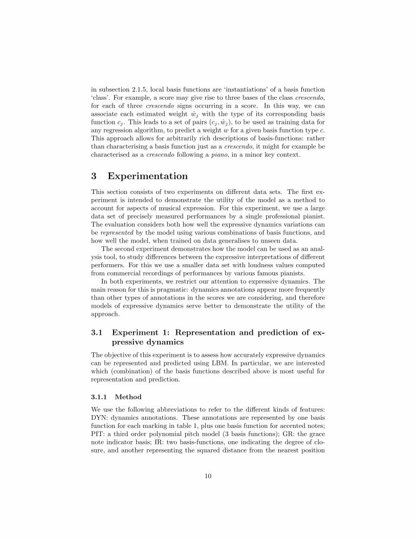
3.1 Experiment 1: Representation and prediction of ex-pressive dynamics

The objective of this experiment is to assess how accurately expressive dynamicscan be represented and predicted using LBM. In particular, we are interestedwhich (combination) of the basis functions described above is most useful forrepresentation and prediction.

3.1.1 Method

We use the following abbreviations to refer to the different kinds of features:DYN: dynamics annotations. These annotations are represented by one basisfunction for each marking in table 1, plus one basis function for accented notes;PIT: a third order polynomial pitch model (3 basis functions); GR: the gracenote indicator basis; IR: two basis-functions, one indicating the degree of clo-sure, and another representing the squared distance from the nearest position

10

where closure occurs. The latter feature forms arch-like parabolic structuresreminiscent of Todd’s (1992) model of dynamics.

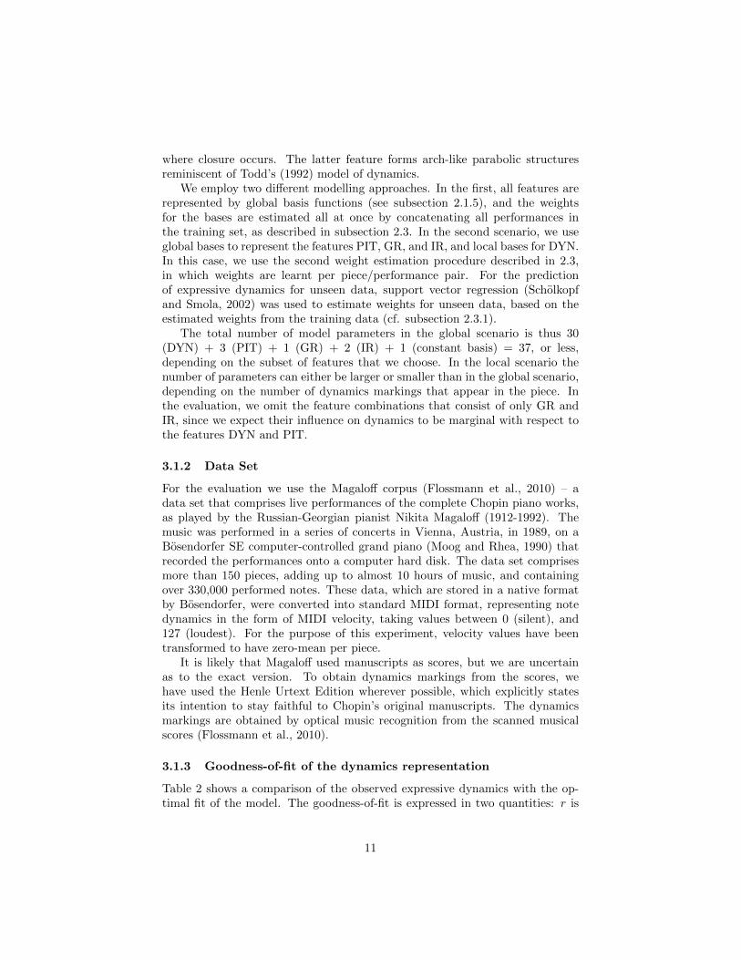
We employ two different modelling approaches. In the first, all features arerepresented by global basis functions (see subsection 2.1.5), and the weightsfor the bases are estimated all at once by concatenating all performances inthe training set, as described in subsection 2.3. In the second scenario, we useglobal bases to represent the features PIT, GR, and IR, and local bases for DYN.In this case, we use the second weight estimation procedure described in 2.3,in which weights are learnt per piece/performance pair. For the predictionof expressive dynamics for unseen data, support vector regression (Scholkopfand Smola, 2002) was used to estimate weights for unseen data, based on theestimated weights from the training data (cf. subsection 2.3.1).

The total number of model parameters in the global scenario is thus 30(DYN) + 3 (PIT) + 1 (GR) + 2 (IR) + 1 (constant basis) = 37, or less,depending on the subset of features that we choose. In the local scenario thenumber of parameters can either be larger or smaller than in the global scenario,depending on the number of dynamics markings that appear in the piece. Inthe evaluation, we omit the feature combinations that consist of only GR andIR, since we expect their influence on dynamics to be marginal with respect tothe features DYN and PIT.

3.1.2 Data Set

For the evaluation we use the Magaloff corpus (Flossmann et al., 2010) – adata set that comprises live performances of the complete Chopin piano works,as played by the Russian-Georgian pianist Nikita Magaloff (1912-1992). Themusic was performed in a series of concerts in Vienna, Austria, in 1989, on aBosendorfer SE computer-controlled grand piano (Moog and Rhea, 1990) thatrecorded the performances onto a computer hard disk. The data set comprisesmore than 150 pieces, adding up to almost 10 hours of music, and containingover 330,000 performed notes. These data, which are stored in a native formatby Bosendorfer, were converted into standard MIDI format, representing notedynamics in the form of MIDI velocity, taking values between 0 (silent), and127 (loudest). For the purpose of this experiment, velocity values have beentransformed to have zero-mean per piece.

It is likely that Magaloff used manuscripts as scores, but we are uncertainas to the exact version. To obtain dynamics markings from the scores, wehave used the Henle Urtext Edition wherever possible, which explicitly statesits intention to stay faithful to Chopin’s original manuscripts. The dynamicsmarkings are obtained by optical music recognition from the scanned musicalscores (Flossmann et al., 2010).

3.1.3 Goodness-of-fit of the dynamics representation

Table 2 shows a comparison of the observed expressive dynamics with the op-timal fit of the model. The goodness-of-fit is expressed in two quantities: r is

11

r R2

Basis (global) avg. std. avg. std.

DYN 0.332 (0.150) 0.133 (0.117)PIT 0.456 (0.108) 0.219 (0.097)DYN+PIT 0.565 (0.106) 0.330 (0.122)DYN+PIT+GR 0.567 (0.107) 0.332 (0.123)DYN+PIT+IR 0.575 (0.102) 0.341 (0.120)DYN+PIT+GR+IR 0.577 (0.102) 0.343 (0.120)

Basis (local)

DYN 0.497 (0.170) 0.276 (0.160)PIT 0.456 (0.108) 0.219 (0.097)DYN+PIT 0.670 (0.113) 0.462 (0.146)DYN+PIT+GR 0.671 (0.113) 0.463 (0.146)DYN+PIT+IR 0.678 (0.109) 0.471 (0.142)DYN+PIT+IR+GR 0.678 (0.109) 0.472 (0.142)

Table 2: Goodness of fit of the model; See section 3.1 for abbreviations

the Pearson product-moment correlation coefficient, denoting how strongly theobserved dynamics and the dynamics values of the fitted model correlate. Thequantity R2 is the coefficient of determination, which expresses the proportionof variance accounted for by the model.Average and standard deviations (inparentheses) of the r and R2 values over the 154 musical pieces are listed intable 2.

The results show that both the strongest correlation, and the highest coeffi-cient of determination is achieved when using local basis for dynamics markings,and including all features. This is unsurprising, since in the global setting a sin-gle weight vector is used to fit all pieces, whereas in the local setting each piecehas its own weight vector. Furthermore, since adding features increases thenumber of parameters in the model, it will also increase the goodness-of-fit. Wenote however, that the r and R2 values are averaged over pieces, with a consid-erable standard deviation, and that differences between outcomes may not allbe significant.

3.1.4 Predictive accuracy of the model

The additional flexibility of the model, by using local bases and adding fea-tures, may increase its goodness-of-fit. However, it is doubtful that it will helpto obtain good model predictions for unseen musical pieces. To evaluate theaccuracy of the predictions of a trained model for an unseen piece, we perform aleave-one-out cross-validation over the 154 pieces. The predictions are evaluatedagain in terms of averaged r and R2 values over the pieces, which are shown intable 3.

The average correlation coefficients between prediction and observation for

12

r R2

Basis (global) avg. std. avg. std.

DYN 0.192 (0.173) 0.020 (0.100)PIT 0.422 (0.129) 0.147 (0.111)DYN+PIT 0.462 (0.125) 0.161 (0.156)DYN+PIT+GR 0.462 (0.125) 0.161 (0.156)DYN+PIT+IR 0.462 (0.124) 0.162 (0.155)DYN+PIT+GR+IR 0.462 (0.124) 0.162 (0.154)

Basis (local)

DYN 0.192 (0.179) 0.024 (0.109)PIT 0.415 (0.137) 0.149 (0.149)DYN+PIT 0.459 (0.126) 0.151 (0.220)DYN+PIT+GR 0.459 (0.123) 0.153 (0.195)DYN+PIT+IR 0.455 (0.130) 0.141 (0.231)DYN+PIT+IR+GR 0.457 (0.123) 0.188 (0.126)

Table 3: Predictive accuracy the model in a leave-one-out scenario; See sec-tion 3.1 for abbreviations

the local and global basis settings are roughly similar, ranging from weak (r =.19) to medium correlation (r = .46). In the global setting, increasing the com-plexity of the model does not affect its predictive accuracy, whereas in the localsetting, maximal predictive accuracy is achieved for models of moderate com-plexity (including dynamics, pitch, and grace note information). The decreaseof accuracy for more complex models is likely to be caused by overfitting.

Interestingly, the highest proportion of explained variance (R2 = .19) isachieved by the predictions of the local model with all available features (DYN+PIT+IR+GR).Note however, that the standard deviation of R2 is large in most cases.

3.2 Experiment 2: Analysis of expressive dynamics incommercial recordings

The above experiments are all done using the performances of a single performer.In the next experiment, we wish to highlight that the LBM framework can alsobe used to study differences between performers.

3.2.1 Method

Given the performances of a number of pieces by different performers, we fit anLBM to the expressive dynamics in the performances. The fitted weights arethen compared across pieces and performers.

By the nature of the data (see subsection 3.2.2), loudness measurements areonly available on a beat level. Moreover the measurements are only approximate,

13

Piece PerformancesOp. 52 Kissin1998, Pollini1999, Zimerman1987, Horowitz1952/1981,

Rubinstein1959, Cherkassky1987, Ashkenazy1964, Perahia1994Op. 15(1) Ashkenazy1985, Rubinstein1965, Richter1968, Maisenberg1995,

Leonskaja1992, Arrau1978, Harasiewicz1961, Pollini1968,Barenboim1981, Pires1996, Argerich1965, Horowitz1957, Per-ahia1994

Op. 27(2) Rubinstein1965, Arrau1978, Kissin1993, Leonskaja1992,Pollini1968, Barenboim1981, Ashkenazy1985, Pires1996,Harasiewicz1961

Op. 28(17) Sokolov1990, Arrau1973, Harasiewicz1963, Pogorelich1989,Argerich1975, Ashkenazy1985, Rubinstein1946, Pires1992,Kissin1999, Pollini1975

Table 4: Performances used for evaluation

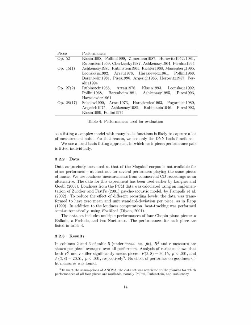
so a fitting a complex model with many basis-functions is likely to capture a lotof measurement noise. For that reason, we use only the DYN basis functions.

We use a local basis fitting approach, in which each piece/performance pairis fitted individually.

3.2.2 Data

Data as precisely measured as that of the Magaloff corpus is not available forother performers – at least not for several performers playing the same piecesof music. We use loudness measurements from commercial CD recordings as analternative. The data for this experiment has been used earlier by Langner andGoebl (2003). Loudness from the PCM data was calculated using an implemen-tation of Zwicker and Fastl’s (2001) psycho-acoustic model, by Pampalk et al.(2002). To reduce the effect of different recording levels, the data was trans-formed to have zero mean and unit standard-deviation per piece, as in Repp(1999). In addition to the loudness computation, beat-tracking was performedsemi-automatically, using BeatRoot (Dixon, 2001).

The data set includes multiple performances of four Chopin piano pieces: aBallade, a Prelude, and two Nocturnes. The performances for each piece arelisted in table 4.

3.2.3 Results

In columns 2 and 3 of table 5 (under meas. vs. fit), R2 and r measures areshown per piece, averaged over all performers. Analysis of variance shows thatboth R2 and r differ significantly across pieces: F (3, 8) = 30.15, p < .001, andF (3, 8) = 26.51, p < .001, respectively5. No effect of performer on goodness-of-fit measures was found.

5To meet the assumptions of ANOVA, the data set was restricted to the pianists for whichperformances of all four pieces are available, namely Pollini, Rubinstein, and Ashkenazy

14

-2

-1

0

1

2

3

0 24 48 72 96 120 144 168 192 216 240 264 288 312 336 360 384 408 432 456 480 504 528

Loud

ness

(S

one,

norm

aliz

ed

)

Score time (8th notes)

Rubinstein, 1946Model approximation

<

p >

f cresc

dim

<

<

<

cresff

p <

<

<

<dim

<

f

<

>pp

fz fz fz fz fz fz fz fz

perdendosi

fz fz< >

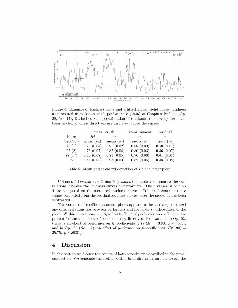
Figure 4: Example of loudness curve and a fitted model; Solid curve: loudnessas measured from Rubinstein’s performance (1946) of Chopin’s Prelude (Op.28, No. 17); Dashed curve: approximation of the loudness curve by the linearbasis model; loudness directives are displayed above the curves

meas. vs. fit measurement residualPiece R2 r r r

Op.(No.) mean (sd) mean (sd) mean (sd) mean (sd)15 (1) 0.90 (0.04) 0.95 (0.02) 0.88 (0.03) 0.50 (0.11)27 (2) 0.76 (0.07) 0.87 (0.04) 0.80 (0.03) 0.56 (0.07)28 (17) 0.66 (0.08) 0.81 (0.05) 0.76 (0.06) 0.61 (0.05)

52 0.86 (0.05) 0.93 (0.03) 0.82 (0.06) 0.48 (0.08)

Table 5: Mean and standard deviation of R2 and r per piece

Columns 4 (measurement) and 5 (residual) of table 5 summarise the cor-relations between the loudness curves of performers. The r values in column4 are computed on the measured loudness curves. Column 5 contains the rvalues computed from the residual loudness curves, after the model fit has beensubtracted.

The variance of coefficients across pieces appears to be too large to revealany direct relationships between performers and coefficients, independent of thepiece. Within pieces however, significant effects of performer on coefficients arepresent for the coefficients of some loudness directives. For example, in Op. 52.there is an effect of performer on ff coefficients (F (7, 28) = 3.90, p < .005),and in Op. 28 (No. 17), an effect of performer on fz coefficients (F (9, 90) =25.75, p < .0001).

4 Discussion

In this section we discuss the results of both experiments described in the previ-ous section. We conclude the section with a brief discussion on how we see the

15

LBM framework in relation to creative aspects of expressive music performance.

4.1 Discussion of experiment 1

The results presented in experiment 1 show a substantial difference in the con-tribution of dynamical annotations (DYN) and pitch (PIT) to the performanceof the model. The fact that pitch explains a larger proportion of the dynamicsvariance than the annotations may be surprising, given that annotations are bynature intended to guide dynamics. One may hypothesise that the effect of pitchon dynamics is due to the fact that on a piano different keys must be struckwith different intensities to achieve the same sound pressure level (SPL) Goebland Bresin (2003). However, on the Bosendorfer, the pitches around C5 (midivalue 72) produce a higher SPL at the same MIDI velocity than lower pitches.Thus, the pitch effect on dynamics is not a matter of SPL compensation.

Although the data set contains many performances, it is important to realisethat the results are derived from performances of a single performer, performingthe music of a single composer. The importance of pitch as a predictor fordynamics may be different for other performers, composers, and musical genres.Specifically, we hypothesise that the fact that pitch effect on dynamics is aconsequence of melody lead. This phenomenon, which has been the subjectof extensive study (see Repp (1996); Goebl (2001)), consists in the consistenttendency of pianists to play melody notes both louder and slightly earlier thanthe accompaniment. This makes the melody more clearly recognisable by thelistener, and may improve the sensation of a coherent musical structure. Inmany musical genres, the main melody of the music is expressed in the highestvoice, which explains the relationship between pitch and dynamics.

This effect is clearly visible in figure 5, which displays observed, fitted, andpredicted dynamics for the final measures of Chopin’s Prelude in B major (Opus28, No. 11). In this plot, the velocity of simultaneous notes is plotted at different(adjacent) positions on the horizontal axis, for the ease of interpretation. Melodynotes are indicated with dotted vertical lines. It is easily verified by eye that thevelocity of melody notes is substantially higher than the velocity of non-melodynotes. This effect is very prominent in the predictions of the model as well. 6

Although observed and predicted dynamics are visibly correlated, figure 5shows that the variance of the prediction is substantially lower than that ofthe observation, meaning that expressive effects in the predicted performanceare less pronounced. The lower variance is most likely caused by the fact thatthe model parameters have been optimised to performances of a wide range ofdifferent pieces, preventing the model from accurately capturing dynamics inindividual performances. This suggests a separate treatment of musical pieceswith distinct musical characters.

6See www.cp.jku.at/research/TRP109-N23/BasisMixer/midis.html for sound examples

16

-30

-20

-10

0

10

20

30

200 220 240 260 280 300

Nor

mal

ized

Lou

dnes

s (M

IDI v

eloc

ity)

Notes (simultaneous notes layed out horizontally)

MagaloffLinear Basis Model - Optimal fit

Linear Basis Model - Prediction (leave-one-out)

Figure 5: Observed, fitted, and predicted note-by-note dynamics of Chopin’sPrelude in B major (Opus 28, No. 11), from measure 16 onwards; Fitting andprediction was done using the global bases DYN+PIT+GR+IR (see section 3.1);Vertical dotted lines indicate melody notes

4.2 Discussion of experiment 2

The results of experiment 2 show that the LBM in combination with DYNbasis functions accounts for a large part of dynamics in music performances(66%–90%, depending on the piece; see table 5). The residual loudness aftersubtracting model fits is substantially less correlated between performers. Theremaining correlation is an indication of factors that are not represented bythe model. Obvious candidates are pitch, and the number of simultaneouslysounding notes.

It is unlikely however, that the described method in its current form willresult in clear ‘coefficient profiles’ of performers, i.e. sets of coefficients thatuniquely characterise how a performer interprets annotations. Many decisionson how to interpret annotations will depend on the context of the annotationand on musical understanding of a level that is not easy to capture in a simplemathematical model.

Nevertheless, LBM can be a useful tool to compare interpretations of differ-ent performers for a particular piece or musical fragment. It provides estimatesof how (strongly) each annotation has shaped the dynamics of the performance.Although the model provides only an approximation of the performed dynamics,these estimates can often be meaningfully compared across performers.

4.3 LBM and creativity in musical expression

The LBM framework presented in this paper is an attempt to account for mu-sical expression in a rather simple manner, namely as a weighted sum of score-

17

determined basis functions. One may wonder whether such a model leaves anyroom for other aspects of musical expression, such as the performer’s expressiveintentions, especially the affective information she wishes to transmit to thelistener.

Theoretically speaking, since the models factorise musical expression intoweights and basis functions, any expressive information should be captured ei-ther in one, or in the other. In this paper, we have treated the basis functions asa fixed part of the model, and the weights as parameters to be fit to data. One(admittedly simplistic) way to conceive of the artistic freedom of performers, isto regard the weights as a “palette” with which performers “colour” the per-formance differently, depending on which basis functions receive high weights.This idea has been proposed for a system of rules for musical expression (Bresinand Friberg, 2000).

It is also plausible that expressive variation due to affective intentions, orindividual performer style, may be better modelled by adapting the basis func-tions. Possibly, the shape of a crescendo, or a ritardando may be affect-specific,or even performer specific. Some evidence for performer-specific final ritardshapes has been found (Grachten and Widmer, 2009). To learn the shape ofbasis functions from data however, constraints must be imposed to avoid thatthe model is under-determined.

It should be stated clearly however, that the LBM framework is intendedas a tool for analysing artifacts, rather than the process that led to these arti-facts. Analogously, the process of creating a new performance by using LBM,should not be seen as modelling a cognitive process, let alone a creative process.Whether a performance created by LBM could be regarded as creative by ahuman listener is a philosophical question. We adhere to the view stated byWidmer et al. (2009), that creativity is in the eye of the beholder. It is evenconceivable that the creativity is not just a (subjective) characteristic of theperformance, but also of the listener’s interpretation, by which she construes anovel and unconventional performance as an enjoyable one.

5 Conclusions and future work

The work presented in this paper corroborates the growing insight in musicperformance research, that even if musical expression is a highly complex phe-nomenon, it is by no means fully unsystematic. We have described a linear basismodelling framework to account for expressive variations in music performance.Several types of basis functions were discussed. Using a relatively small set ofbasis functions, it is possible to account for over 45% variance in the dynamicsof Magaloff’s performances of Chopin piano works. Prediction of performancesusing a model trained on performance data unsurprisingly yields lower values,but substantial positive correlations are still observed.

As an analytical tool, we have used the framework to quantise performancedifferences between performers, and pieces. Results indicate that the varianceacross pieces is too large to identify performer-specific expressive style, but

18

within pieces, some performer-specific expressive effects were identified.The LBM framework can be extended in two important ways. Firstly, we

believe the framework is well-suited to a probabilistic approach, in which priorinformation on the distribution of weights is combined with estimates obtainedfrom performance data. Secondly, a strong limitation of the current model isthat basis functions must be defined manually. Dictionary learning techniquesdeveloped in the field of sparse coding may be used to learn basis-functions fromperformances.

Acknowledgements

This research is supported by the Austrian Research Fund (FWF, Z159 “Wittgen-stein Award”). We are indebted to Mme. Irene Magaloff for her generous per-mission to use the data of her late husband’s performances for our research. Forthis research, we have made extensive use of free software.

References

Bresin, R. and Friberg, A. (2000). Emotional coloring of computer-controlledmusic performances. Computer Music Journal, 24(4):44–63.

Canazza, S., De Poli, G., Drioli, C., Roda, A., and Vidolin, A. (2004). Modelingand control of expressiveness in music performance. Proceedings of the IEEE,92(4):686–701.

Canazza, S., De Poli, G., and Roda, A. (2002). Analysis of expressive intentionsin piano performance. Journal of ITC Sangeet Research Academy, 16:23–62.

Clarke, E. F. (1988). Generative principles in music. In Sloboda, J., editor, Gen-erative Processes in Music: The Psychology of Performance, Improvisation,and Composition. Oxford University Press.

Dixon, S. (2001). Automatic extraction of tempo and beat from expressiveperformances. Journal of New Music Research, 30(1):39–58.

Flossmann, S., Goebl, W., Grachten, M., Niedermayer, B., and Widmer, G.(2010). The Magaloff Project: An Interim Report. Journal of New MusicResearch, 39(4):369–377.

Goebl, W. (2001). Melody lead in piano performance: expressive device orartifact? Journal of the Acoustical Society of America, 110(1):563–572.

Goebl, W. and Bresin, R. (2003). Measurement and reproduction accuracyof computer controlled grand pianos. Journal of the Acoustical Society ofAmerica, 114(4):2273–2283.

Good, M. (2001). MusicXML for notation and analysis. In Hewlett, W. B.and Selfridge-Field, E., editors, The Virtual Score: Representation, Retrieval,

19

Restoration, volume 12 of Computing in Musicology, pages 113–124. MITPress, Cambridge, MA.

Grachten, M. (2006). Expressivity-aware Tempo Transformations of Music Per-formances Using Case Based Reasoning. PhD thesis, Pompeu Fabra Univer-sity, Barcelona, Spain. ISBN: 635-07-094-0.

Grachten, M. and Widmer, G. (2009). Who is who in the end? recognizingpianists by their final ritardandi. In Proceedings of the 6th Sound and MusicComputing Conference (SMC), Porto, Portugal.

Grachten, M. and Widmer, G. (2011). Explaining expressive dynamics as amixture of basis functions. In Proceedings of the Eighth Sound and MusicComputing Conference (SMC), Padua, Italy.

Krebs, F. and Grachten, M. (2012). Combining score and filter based models topredict tempo fluctuations in expressive music performances. In Proceedingsof the Ninth Sound and Music Computing Conference (SMC), Copenhagen,Denmark.

Langner, J. and Goebl, W. (2003). Visualizing expressive performance in tempo-loudness space. Computer Music Journal, 27(4):69–83.

Moog, R. A. and Rhea, T. L. (1990). Evolution of the Keyboard Interface: TheBosendorfer 290 SE Recording Piano and the Moog Multiply-Touch-SensitiveKeyboards. Computer Music Journal, 14(2):52–60.

Narmour, E. (1990). The analysis and cognition of basic melodic structures :the Implication-Realization model. University of Chicago Press.

Palmer, C. (1996). Anatomy of a performance: Sources of musical expression.Music Perception, 13(3):433–453.

Palmer, C. (1997). Music performance. Annual Review of Psychology, 48:115–138.

Pampalk, E., Rauber, A., and Merkl, D. (2002). Content-based organization andvisualization of music archives. In Proceedings of the 10th ACM InternationalConference on Multimedia, pages 570–579. ACM.

Parncutt, R. (2003). Perspektiven und Methoden einer Systemischen Musik-wissenschaft, chapter Accents and expression in piano performance, pages163–185. Peter Lang, Germany.

Repp, B. H. (1996). Patterns of note onset asynchronies in expressive pianoperformance. Journal of the Acoustical Society of America, 100(6):3917–3932.

Repp, B. H. (1999). A microcosm of musical expression: II. Quantitative analy-sis of pianists dynamics in the initial measures of Chopin’s Etude in E major.Journal of the Acoustical Society of America, 105(3):1972–1988.

20

Rosenblum, S. P. (1988). Performance practices in classic piano music: theirprinciples and applications. Indiana University Press.

Scholkopf, B. and Smola, A. J. (2002). Learning with Kernels. MIT Press.

Timmers, R.and Ashley, R., Desain, P., Honing, H., and Windsor, L. (2002).Timing of ornaments in the theme of Beethoven’s Paisiello Variations: Em-pirical data and a model. Music Perception, 20(1):3–33.

Tobudic, A. and Widmer, G. (2003). Playing Mozart phrase by phrase. InProceedings of the Fifth International Conference on Case-Based Reasoning(ICCBR-03), number 2689 in Lecture Notes in Artificial Intelligence, pages552–566. Springer-Verlag.

Todd, N. (1992). The dynamics of dynamics: A model of musical expression.Journal of the Acoustical Society of America, 91:3540–3550.

Widmer, G., Flossmann, S., and Grachten, M. (2009). YQX plays Chopin. AIMagazine (Special Issue on Computational Creativity), 30(3):35–48.

Zwicker, E. and Fastl, H. (2001). Psychoacoustics: Facts and Models. Springer-Verlag, Berlin, 2nd edition.

21