linear maps, the total derivative and the chain rule

LINEAR MAPS, THE TOTAL DERIVATIVE AND THE CHAIN RULE

ROBERT LIPSHITZ

Abstract. We will discuss the notion of linear maps and introduce the total derivative ofa function f : Rn → Rm as a linear map. We will then discuss composition of linear mapsand the chain rule for derivatives.

Contents

1. Maps Rn → Rm 12. Linear maps 53. Matrices 84. The total derivative and the Jacobian matrix 104.1. Review of the derivative as linear approximation 104.2. The total derivative of a function Rn → Rm 124.3. The Jacobian matrix 145. Composition of linear maps and matrix multiplication 155.1. Matrix arithmetic 186. The chain rule for total derivatives 196.1. Comparison with the treatment in Stewart’s Calculus 22

1. Maps Rn → Rm

So far in this course, we have talked about:

• Functions R→ R; you worked with these a lot in Calculus 1.• Parametric curves, i.e., functions R→ R2 and R→ R3, and• Functions of several variables, i.e., functions R2 → R and R3 → R.

(We’ve probably also seen some examples of maps Rn → R for some n > 3, but we haven’tworked with these so much.)

What we haven’t talked about much are functions R3 → R3, say, or R3 → R2, or R2 → R2.

Definition 1.1. A function f : R3 → R3 is something which takes as input a vector in R3

and gives as output a vector in R3. Similarly, a map R3 → R2 takes as input a vector in R3

and gives as output a vector in R2; and so on.

Example 1.2. Rotation by π/6 counter-clockwise around the z-axis is a function R3 → R3:it takes as input a vector in R3 and gives as output a vector in R3. Let’s let R(~v) denoterotation of ~v by π/6 counter-clockwise around the z-axis. Then, doing some trigonometry

Copyright 2009 by Robert Lipshitz. Released under the Creative Commons Attribution-Noncommercial-Share Alike 3.0 Unported License.

1

2 ROBERT LIPSHITZ

(see Figure 1 for the two-dimensional analogue), we have for example

R(1, 0, 0) = (cos(π/6), sin(π/6), 0) = (√

3/2, 1/2, 0)

R(0, 1, 0) = (− sin(π/6), cos(π/6), 0)(−1/2,√

3/2, 0)

R(0, 0, 1) = (0, 0, 1)

R(2, 3, 1) = (2 cos(π/6)− 3 sin(π/6), 2 sin(π/6) + 3 cos(π/6), 1).

Example 1.3. Translation by the vector (1, 2, 3) is a map R3 → R3: it takes as input anyvector ~v and gives as output ~v+ (1, 2, 3). Let T (~v) denote translation of ~v by (1, 2, 3). Then,for example

T (1, 0, 0) = (2, 2, 3)

T (0, 1, 0) = (1, 3, 3)

T (0, 0, 1) = (1, 2, 4)

T (2, 3, 1) = (3, 5, 4).

Example 1.4. Orthogonal projection from R3 to the xy-plane can be viewed as a functionP : R3 → R2. Then, for example

P (1, 0, 0) = (1, 0)

P (0, 1, 0) = (0, 1)

P (0, 0, 1) = (0, 0)

P (2, 3, 1) = (2, 3).

Example 1.5. Rotation by an angle θ around the origin gives a map Rθ : R2 → R2. Forexample,

Rθ(1, 0) = (cos(θ), sin(θ))

Rθ(0, 1) = (− sin(θ), cos(θ))

Rθ(2, 3) = (2 cos(θ)− 3 sin(θ), 2 sin(θ) + 3 cos(θ)).

(See Figure 1 for the trigonometry leading to the computation of Rθ(2, 3).)

Just like a function R → R3 corresponds to three functions R → R, a function R3 → R3

corresponds to three functions R3 → R. That is, any function F : R3 → R3 is given by

F (x, y, z) = (u(x, y, z), v(x, y, z), w(x, y, z)).

Example 1.6. The function R from Example 1.2 has the form

R(x, y, z) = (x cos(π/6)− y sin(π/6), x sin(π/6) + y cos(π/6), z).

Example 1.7. The function T from Example 1.3 has the form

T (x, y, z) = (x+ 1, y + 2, z + 3).

Example 1.8. There is a function which takes a point written in cylindrical coordinates andrewrites it in rectangular coordinates, which we can view as a map R3 → R3 given by

F (r, θ, z) = (r cos(θ), r sin(θ), z).

Similarly, there is a function which takes a point written in spherical coordinates andrewrites it in rectangular coordinates; viewed as a function R3 → R3 it is given by

G(ρ, θ, φ) = (ρ cos(θ) sin(φ), ρ sin(θ) sin(φ), ρ cos(φ)).

THE TOTAL DERIVATIVE 3

Figure 1. Two derivations of the formula for rotation of R2 by anangle θ. Left: Notice that (x, y) = (x, 0) + (0, y). So, rotating the whole pic-ture, Rθ(x, y) = Rθ(x, 0)+Rθ(0, y) = (x cos(θ), x sin(θ))+(−y sin(θ), y cos(θ)),which is exactly (x cos(θ) − y sin(θ), y cos(θ) + x sin(θ)). Right: the point(x, y) is (r cos(α), r sin(α)) and Rθ(x, y) = (r cos(α + θ), sin(α + θ)). So,by addition formulas for sine and cosine, Rθ(x, y) = (r cos(α) cos(θ) −r sin(α) sin(θ), r sin(α) cos(θ) + r cos(α) sin(θ)) which is exactly (x cos(θ) −y sin(θ), y cos(θ) + x sin(θ)).

Figure 2. Visualizing maps R2 → R2. Left: the effect of the map Rπ/6

from Example 1.5. Right: the effect of the function F (x, y) = (x+ y, y).

Example 1.9. The function Rθ from Example 1.5 is given in coordinates by:

Rθ(x, y) = (x cos(θ)− y sin(θ), x sin(θ) + y cos(θ)).

See Figure 1 for the trigonometry leading to this formula.

Functions R2 → R2 are a little easier to visualize than functions R3 → R3 or R3 → R2

(or. . . ). One way to visualize them is to think of how they transform a picture. A couple ofexamples are illustrated in Figure 2.

Given functions F : Rp → Rn and G : Rn → Rm you can compose F and G to get a newfunction G ◦ F : Rp → Rm. That is, G ◦ F is the function which takes a vector ~v, does F to~v, and then does G to the result; symbolically, G ◦ F (~v) = G(F (v)).

Note that G ◦ F only makes sense if the target of F is the same as the source of G.

4 ROBERT LIPSHITZ

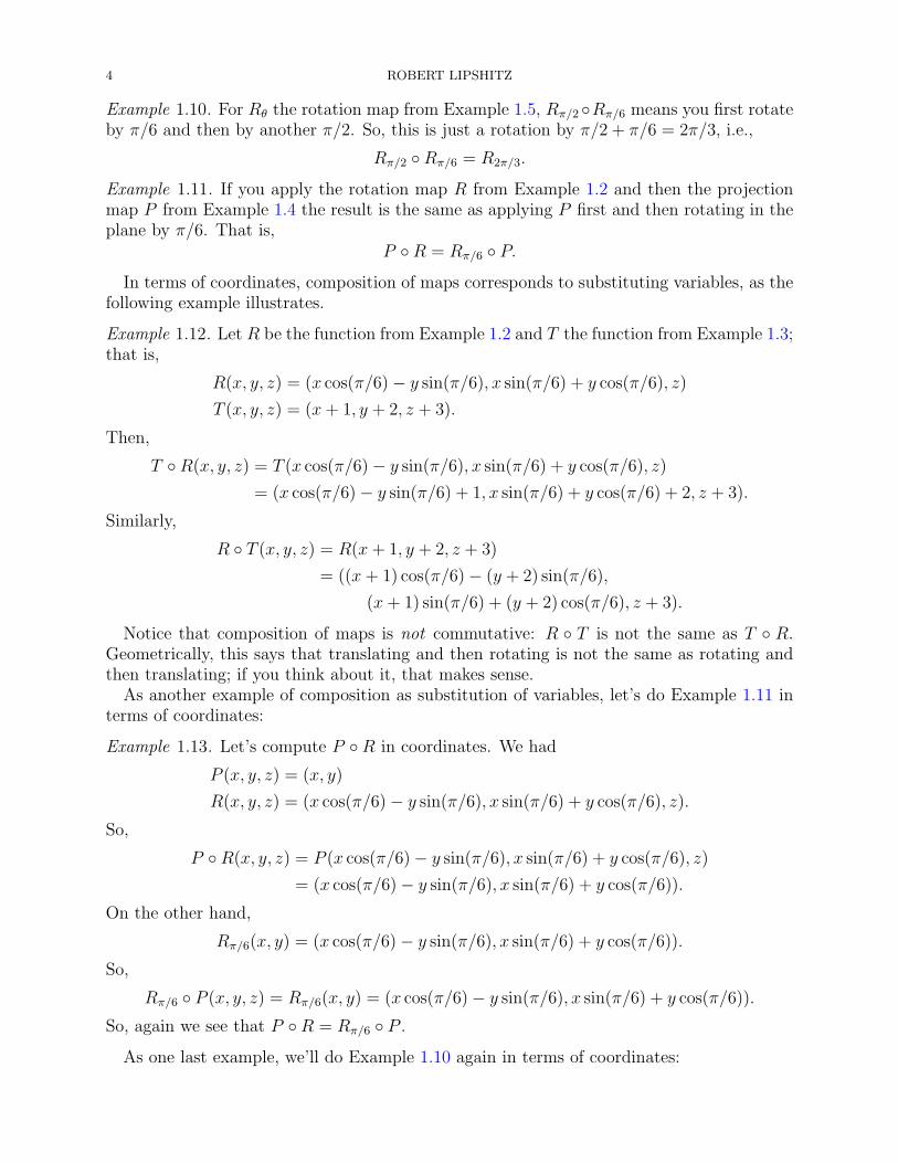
Example 1.10. For Rθ the rotation map from Example 1.5, Rπ/2 ◦Rπ/6 means you first rotateby π/6 and then by another π/2. So, this is just a rotation by π/2 + π/6 = 2π/3, i.e.,

Rπ/2 ◦Rπ/6 = R2π/3.

Example 1.11. If you apply the rotation map R from Example 1.2 and then the projectionmap P from Example 1.4 the result is the same as applying P first and then rotating in theplane by π/6. That is,

P ◦R = Rπ/6 ◦ P.

In terms of coordinates, composition of maps corresponds to substituting variables, as thefollowing example illustrates.

Example 1.12. Let R be the function from Example 1.2 and T the function from Example 1.3;that is,

R(x, y, z) = (x cos(π/6)− y sin(π/6), x sin(π/6) + y cos(π/6), z)

T (x, y, z) = (x+ 1, y + 2, z + 3).

Then,

T ◦R(x, y, z) = T (x cos(π/6)− y sin(π/6), x sin(π/6) + y cos(π/6), z)

= (x cos(π/6)− y sin(π/6) + 1, x sin(π/6) + y cos(π/6) + 2, z + 3).

Similarly,

R ◦ T (x, y, z) = R(x+ 1, y + 2, z + 3)

= ((x+ 1) cos(π/6)− (y + 2) sin(π/6),

(x+ 1) sin(π/6) + (y + 2) cos(π/6), z + 3).

Notice that composition of maps is not commutative: R ◦ T is not the same as T ◦ R.Geometrically, this says that translating and then rotating is not the same as rotating andthen translating; if you think about it, that makes sense.

As another example of composition as substitution of variables, let’s do Example 1.11 interms of coordinates:

Example 1.13. Let’s compute P ◦R in coordinates. We had

P (x, y, z) = (x, y)

R(x, y, z) = (x cos(π/6)− y sin(π/6), x sin(π/6) + y cos(π/6), z).

So,

P ◦R(x, y, z) = P (x cos(π/6)− y sin(π/6), x sin(π/6) + y cos(π/6), z)

= (x cos(π/6)− y sin(π/6), x sin(π/6) + y cos(π/6)).

On the other hand,

Rπ/6(x, y) = (x cos(π/6)− y sin(π/6), x sin(π/6) + y cos(π/6)).

So,

Rπ/6 ◦ P (x, y, z) = Rπ/6(x, y) = (x cos(π/6)− y sin(π/6), x sin(π/6) + y cos(π/6)).

So, again we see that P ◦R = Rπ/6 ◦ P .

As one last example, we’ll do Example 1.10 again in terms of coordinates:


Example 1.14. We have

Rπ/2(x, y) = (x cos(π/2)− y sin(π/2), x sin(π/2) + y cos(π/2)) = (−y, x)

Rπ/6(x, y) = (x cos(π/6)− y sin(π/6), x sin(π/6) + y cos(π/6))

= (x√

3/2− y/2, x/2 + y√

3/2)

R2π/3(x, y) = (x cos(2π/3)− y sin(2π/3), x sin(2π/3) + y cos(2π/3))

= (−x/2− y√

3/2, x√

3/2− y/2).

Composing Rπ/2 and Rπ/6 we get

Rπ/2 ◦Rπ/6(x, y) = Rπ/2(x√

3/2− y/2, x/2 + y√

3/2) = (−x/2− y√

3/2, x√

3/2− y/2).

So, again we see that Rπ/2 ◦Rπ/6 = R2π/3.

Exercise 1.15. Let T be the map from Example 1.3. What does the map T ◦ T meangeometrically? What is it in coordinates?

Exercise 1.16. Let F be the “write cylindrical coordinates in rectangular coordinates” mapfrom Example 1.8. Let H(r, θ, z) = (r, θ + π/6, z). Compute F ◦H in coordinates.

Exercise 1.17. Let Rθ be the rotation map from Example 1.5. Compose Rθ and Rφ bysubstituting, like in Example 1.14.

We also know that Rφ ◦Rθ = Rθ+φ. Deduce the formulas for sin(θ + φ) and cos(θ + φ).

2. Linear maps

We’ll start with a special case:

Definition 2.1. A map F : R2 → R2 is linear if F can be written in the form

F (x, y) = (ax+ by, cx+ dy)

for some real numbers a, b, c, d.

That is, a linear map is one given by homogeneous linear equations:

xnew = axold + byold

ynew = cxold + dyold.

(The word homogeneous means that there are no constant terms.)

Example 2.2. The map f(x, y) = (2x+ 3y, x+ y) is a linear map R2 → R2.

Example 2.3. The map Rπ/2 : R2 → R2 which is rotation by the angle π/2 around the originis a linear map: it is given in coordinates as

Rπ/2(x, y) = (−y, x) = (0x+ (−1)y, 1x+ 0y).

Example 2.4. More generally, the map Rθ : R2 → R2 which is rotation by the angle θ aroundthe origin is a linear map: it is given in coordinates as

Rθ(x, y) = (cos(θ)x− sin(θ)y, sin(θ)x+ cos(θ)y).

(Notice that cos(θ) and sin(θ) are constants, so it’s fine for them to be coefficients in a linearmap.)

More generally:

6 ROBERT LIPSHITZ

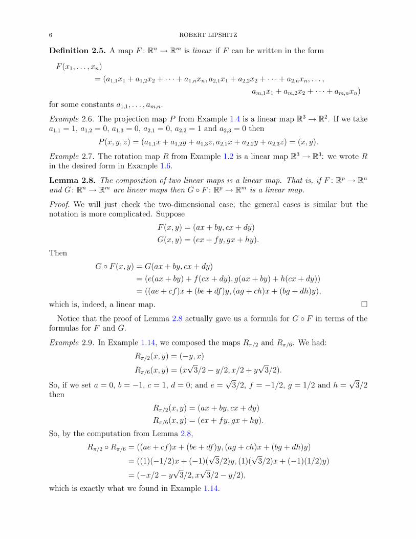
Definition 2.5. A map F : Rn → Rm is linear if F can be written in the form

F (x1, . . . , xn)

= (a1,1x1 + a1,2x2 + · · ·+ a1,nxn, a2,1x1 + a2,2x2 + · · ·+ a2,nxn, . . . ,

am,1x1 + am,2x2 + · · ·+ am,nxn)

for some constants a1,1, . . . , am,n.

Example 2.6. The projection map P from Example 1.4 is a linear map R3 → R2. If we takea1,1 = 1, a1,2 = 0, a1,3 = 0, a2,1 = 0, a2,2 = 1 and a2,3 = 0 then

P (x, y, z) = (a1,1x+ a1,2y + a1,3z, a2,1x+ a2,2y + a2,3z) = (x, y).

Example 2.7. The rotation map R from Example 1.2 is a linear map R3 → R3: we wrote Rin the desired form in Example 1.6.

Lemma 2.8. The composition of two linear maps is a linear map. That is, if F : Rp → Rn

and G : Rn → Rm are linear maps then G ◦ F : Rp → Rm is a linear map.

Proof. We will just check the two-dimensional case; the general cases is similar but thenotation is more complicated. Suppose


G(x, y) = (ex+ fy, gx+ hy).

Then

G ◦ F (x, y) = G(ax+ by, cx+ dy)

= (e(ax+ by) + f(cx+ dy), g(ax+ by) + h(cx+ dy))

= ((ae+ cf)x+ (be+ df)y, (ag + ch)x+ (bg + dh)y),

which is, indeed, a linear map. �

Notice that the proof of Lemma 2.8 actually gave us a formula for G ◦ F in terms of theformulas for F and G.

Example 2.9. In Example 1.14, we composed the maps Rπ/2 and Rπ/6. We had:

Rπ/2(x, y) = (−y, x)

Rπ/6(x, y) = (x√

3/2− y/2, x/2 + y√

3/2).

So, if we set a = 0, b = −1, c = 1, d = 0; and e =√

3/2, f = −1/2, g = 1/2 and h =√

3/2then

Rπ/2(x, y) = (ax+ by, cx+ dy)

Rπ/6(x, y) = (ex+ fy, gx+ hy).

So, by the computation from Lemma 2.8,

Rπ/2 ◦Rπ/6 = ((ae+ cf)x+ (be+ df)y, (ag + ch)x+ (bg + dh)y)

= ((1)(−1/2)x+ (−1)(√

3/2)y, (1)(√

3/2)x+ (−1)(1/2)y)

= (−x/2− y√

3/2, x√

3/2− y/2),

which is exactly what we found in Example 1.14.


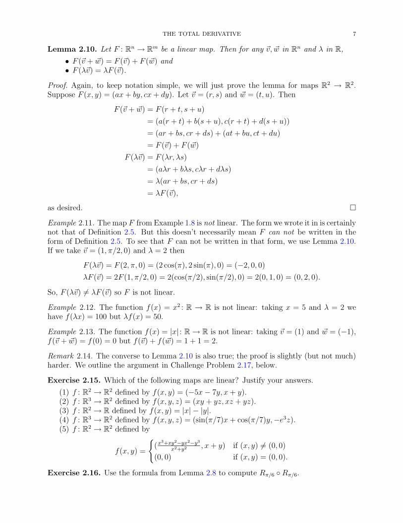
Lemma 2.10. Let F : Rn → Rm be a linear map. Then for any ~v, ~w in Rn and λ in R,

• F (~v + ~w) = F (~v) + F (~w) and• F (λ~v) = λF (~v).

Proof. Again, to keep notation simple, we will just prove the lemma for maps R2 → R2.Suppose F (x, y) = (ax+ by, cx+ dy). Let ~v = (r, s) and ~w = (t, u). Then

F (~v + ~w) = F (r + t, s+ u)

= (a(r + t) + b(s+ u), c(r + t) + d(s+ u))

= (ar + bs, cr + ds) + (at+ bu, ct+ du)

= F (~v) + F (~w)

F (λ~v) = F (λr, λs)

= (aλr + bλs, cλr + dλs)

= λ(ar + bs, cr + ds)

= λF (~v),

as desired. �

Example 2.11. The map F from Example 1.8 is not linear. The form we wrote it in is certainlynot that of Definition 2.5. But this doesn’t necessarily mean F can not be written in theform of Definition 2.5. To see that F can not be written in that form, we use Lemma 2.10.If we take ~v = (1, π/2, 0) and λ = 2 then

F (λ~v) = F (2, π, 0) = (2 cos(π), 2 sin(π), 0) = (−2, 0, 0)

λF (~v) = 2F (1, π/2, 0) = 2(cos(π/2), sin(π/2), 0) = 2(0, 1, 0) = (0, 2, 0).

So, F (λ~v) 6= λF (~v) so F is not linear.

Example 2.12. The function f(x) = x2 : R → R is not linear: taking x = 5 and λ = 2 wehave f(λx) = 100 but λf(x) = 50.

Example 2.13. The function f(x) = |x| : R→ R is not linear: taking ~v = (1) and ~w = (−1),f(~v + ~w) = f(0) = 0 but f(~v) + f(~w) = 1 + 1 = 2.

Remark 2.14. The converse to Lemma 2.10 is also true; the proof is slightly (but not much)harder. We outline the argument in Challenge Problem 2.17, below.

Exercise 2.15. Which of the following maps are linear? Justify your answers.

(1) f : R2 → R2 defined by f(x, y) = (−5x− 7y, x+ y).(2) f : R3 → R2 defined by f(x, y, z) = (xy + yz, xz + yz).(3) f : R2 → R defined by f(x, y) = |x| − |y|.(4) f : R3 → R2 defined by f(x, y, z) = (sin(π/7)x+ cos(π/7)y,−e3z).(5) f : R2 → R2 defined by

f(x, y) =

{(x

3+xy2−yx2−y3x2+y2

, x+ y) if (x, y) 6= (0, 0)

(0, 0) if (x, y) = (0, 0).

Exercise 2.16. Use the formula from Lemma 2.8 to compute Rπ/6 ◦Rπ/6.

8 ROBERT LIPSHITZ

Challenge Problem 2.17. In this problem we will prove the converse of Lemma 2.10, inthe m = n = 2 case. Suppose that f : R2 → R2 satisfies f(~v + ~w) = f(~v) + f(~w) andf(λ~v) = λf(~v) for any ~v, ~w in R2 and λ in R. Let (a, c) = f(1, 0) and (b, d) = f(0, 1). Provethat for any (x, y), f(x, y) = (ax+ by, cx+ dy).

3. Matrices

Let’s look again at the form of a linear map F from Definition 2.1:

F (x, y) = (ax+ by, cx+ dy).

If we want to specify such a map, all we need to do is specify a, b, c and d: the x and the yare just placeholders. So, we could record this data by writing:

[F ] =

(a bc d

).

This is a matrix, i.e., a rectangular array of numbers. The main point to keep in mind isthat a matrix is just a shorthand for a linear map.1

If we are not just interested in linear maps R2 → R2, our matrices will not be 2× 2. Fora linear map F : Rn → Rm given by

F (x1, . . . , xn)

= (a1,1x1 + a1,2x2 + · · ·+ a1,nxn, a2,1x1 + a2,2x2 + · · ·+ a2,nxn, . . . ,

am,1x1 + am,2x2 + · · ·+ am,nxn),

as in Definition 2.5, the corresponding matrix is

[F ] =

a1,1 a1,2 · · · a1,n

a2,1 a2,2 · · · a2,n...

.... . .

...am,1 am,2 · · · am,n

.

Notice that this matrix has m rows and n columns. Again: the matrix for a linear mapF : Rn → Rm is an m × n matrix. (Notice also that I am writing [F ] to denote the matrixfor F .)

Example 3.1. Suppose P is the projection map from Example 1.4. Then the matrix for P is

[P ] =

(1 0 00 1 0

).

Notice that [P ] is a 2× 3 matrix, and P maps R3 → R2.

Example 3.2. If R is the rotation map from Example 1.2 then the matrix for R is

[R] =

cos(π/6) − sin(π/6) 0sin(π/6) cos(π/6) 0

0 0 1

=

√3/2 −1/2 0

1/2√

3/2 00 0 1

.

Notice that [R] is a 3× 3 matrix and R maps R3 → R3.

1There are also other uses of matrices, but their use as stand-ins for linear maps is their most importantuse, and the only way we will use them.


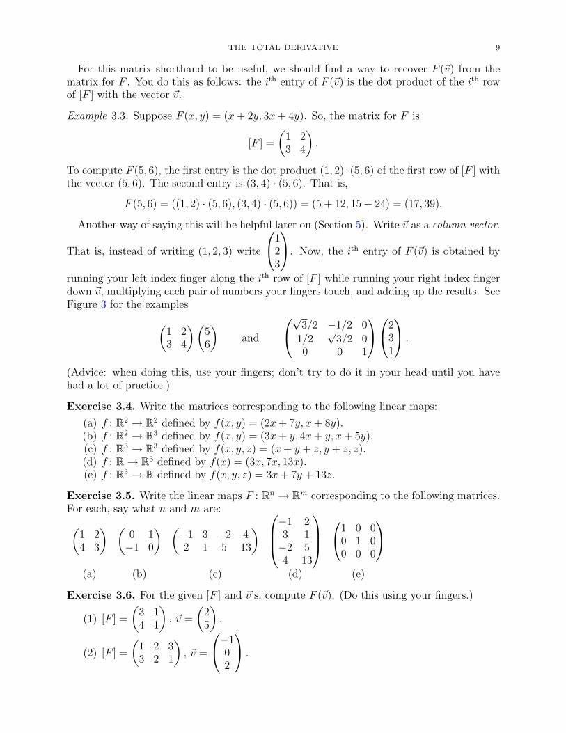
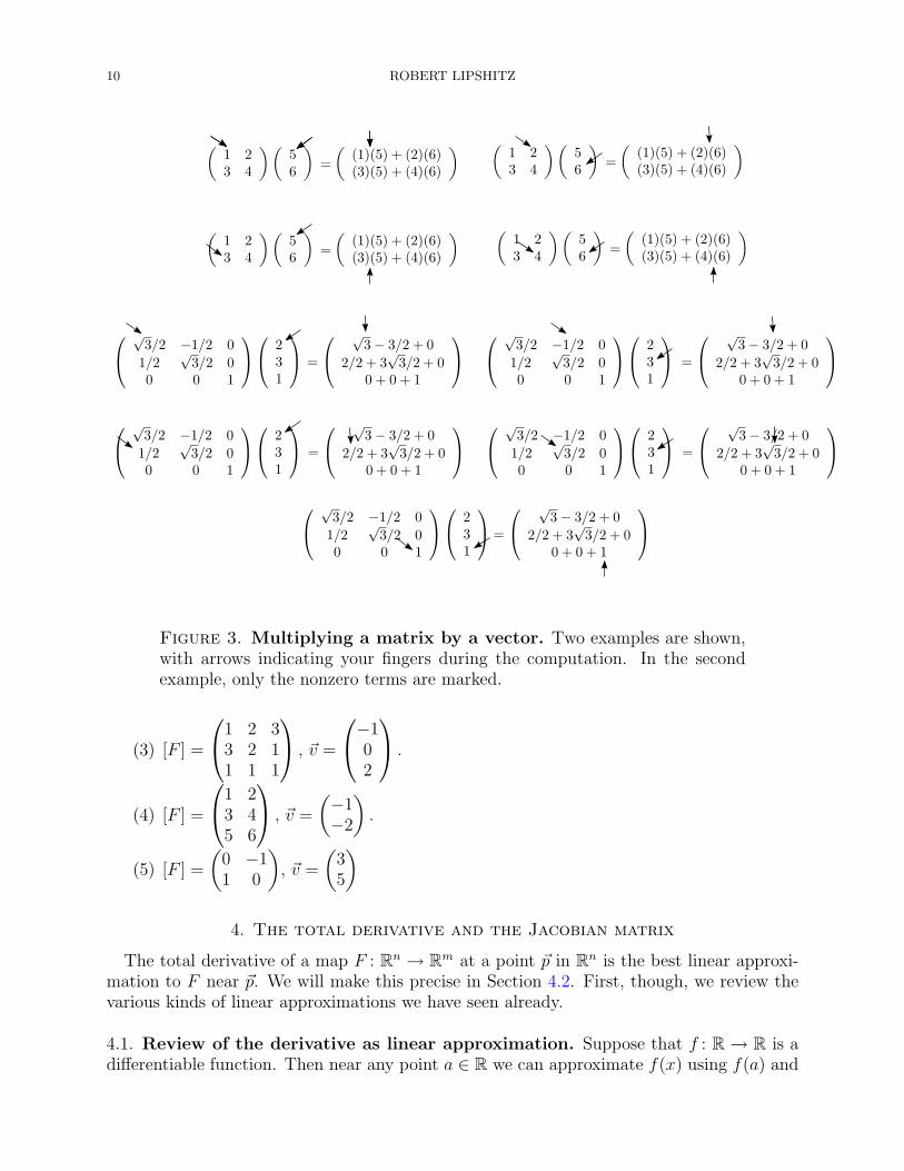
For this matrix shorthand to be useful, we should find a way to recover F (~v) from thematrix for F . You do this as follows: the ith entry of F (~v) is the dot product of the ith rowof [F ] with the vector ~v.

Example 3.3. Suppose F (x, y) = (x+ 2y, 3x+ 4y). So, the matrix for F is

[F ] =

(1 23 4

).

To compute F (5, 6), the first entry is the dot product (1, 2) · (5, 6) of the first row of [F ] withthe vector (5, 6). The second entry is (3, 4) · (5, 6). That is,

F (5, 6) = ((1, 2) · (5, 6), (3, 4) · (5, 6)) = (5 + 12, 15 + 24) = (17, 39).

Another way of saying this will be helpful later on (Section 5). Write ~v as a column vector.

That is, instead of writing (1, 2, 3) write

123

. Now, the ith entry of F (~v) is obtained by

running your left index finger along the ith row of [F ] while running your right index fingerdown ~v, multiplying each pair of numbers your fingers touch, and adding up the results. SeeFigure 3 for the examples(

1 23 4

)(56

)and

√3/2 −1/2 0

1/2√

3/2 00 0 1

231

.

(Advice: when doing this, use your fingers; don’t try to do it in your head until you havehad a lot of practice.)

Exercise 3.4. Write the matrices corresponding to the following linear maps:

(a) f : R2 → R2 defined by f(x, y) = (2x+ 7y, x+ 8y).(b) f : R2 → R3 defined by f(x, y) = (3x+ y, 4x+ y, x+ 5y).(c) f : R3 → R3 defined by f(x, y, z) = (x+ y + z, y + z, z).(d) f : R→ R3 defined by f(x) = (3x, 7x, 13x).(e) f : R3 → R defined by f(x, y, z) = 3x+ 7y + 13z.

Exercise 3.5. Write the linear maps F : Rn → Rm corresponding to the following matrices.For each, say what n and m are:(

1 24 3

) (0 1−1 0

) (−1 3 −2 42 1 5 13

) −1 23 1−2 54 13

1 0 0

0 1 00 0 0

(a) (b) (c) (d) (e)

Exercise 3.6. For the given [F ] and ~v’s, compute F (~v). (Do this using your fingers.)

(1) [F ] =

(3 14 1

), ~v =

(25

).

(2) [F ] =

(1 2 33 2 1

), ~v =

−102

.

10 ROBERT LIPSHITZ

Figure 3. Multiplying a matrix by a vector. Two examples are shown,with arrows indicating your fingers during the computation. In the secondexample, only the nonzero terms are marked.

(3) [F ] =

1 2 33 2 11 1 1

, ~v =

−102

.

(4) [F ] =

1 23 45 6

, ~v =

(−1−2

).

(5) [F ] =

(0 −11 0

), ~v =

(35

)

4. The total derivative and the Jacobian matrix

The total derivative of a map F : Rn → Rm at a point ~p in Rn is the best linear approxi-mation to F near ~p. We will make this precise in Section 4.2. First, though, we review thevarious kinds of linear approximations we have seen already.

4.1. Review of the derivative as linear approximation. Suppose that f : R → R is adifferentiable function. Then near any point a ∈ R we can approximate f(x) using f(a) and


f ′(a):

(4.1) f(a+ h) ≈ f(a) + f ′(a)h.

This is a good approximation in the sense that if we let

ε(h) = f(a+ h)− f(a)− f ′(a)h

denote the error in the approximation (4.1) then ε(h) goes to zero faster than linearly:

limh→0

ε(h)/h = 0.

Similarly, suppose F : R→ Rn is a parametric curve in Rn. If F is differentiable at somea in R then

F (a+ h) ≈ F (a) + F ′(a)h.

This is now a vector equation; the + denotes vector addition and F ′(a)h is scalar mul-tiplication of the vector F ′(a) by the real number h. The sense in which this is a goodapproximation is the same as before: the error goes to 0 faster than linearly. In symbols:

limh→0

F (a+ h)− F (a)− F ′(a)h

h= ~0.

(Again, this is a vector equation now.)As a final special case, consider a function F : Rn → R. To keep notation simple, let’s

consider the case n = 2. Then for any ~a = (a1, a2) in R2,

(4.2) F (~a+ (h1, h2)) ≈ F (~a) +∂F

∂xh1 +

∂F

∂yh2.

Here, the ≈ means that

lim(h1,h2)→(0,0)

F (~a− (h1, h2))− F (~a)− ∂F∂xh1 − ∂F

∂yh2√

h21 + h2

2

= 0.

Notice that we could rewrite Equation (4.2) as

F (~a+ ~h) ≈ F (~a) + (∇F ) · ~h.

The dot product (∇F ) · ~h term looks a lot like matrix multiplication. Indeed, if we defineD~aF to be the linear map with matrix

[D~aF ] =(∂F∂x

∂F∂y

)then Equation (4.2) becomes

F (~a+ ~h) ≈ F (~a) + (D~aF )(~h).

Thus inspired. . .

12 ROBERT LIPSHITZ

4.2. The total derivative of a function Rn → Rm.

Definition 4.3. Let F : Rn → Rm be a map and let ~a be a point in Rn. We say F isdifferentiable at ~a if there is a linear map L : R2 → R2 so that

F (~a+ ~h) ≈ F (~a) + L(~h)

in the sense that

lim~h→~0

F (~a+ ~h)− F (~a)− L(~h)

‖~h‖= ~0.

In this case, we say that L is the total derivative of F at ~a and write DF (~a) to denote L.

Example 4.4. If n = m = 1, so F is a function R → R, then Definition 4.3 agrees with theusual notion, and DF (a) is the map (DF (a))(h) = F ′(a)h. This follows from the discussionin Section 4.1.

Example 4.5. If n = 1, so F is a function R→ Rm then Definition 4.3 agrees with the usualnotion, and DF (a) is the map (DF (a))(h) = hF ′(a) (which is a vector in Rm). Again, thisfollows from the discussion in Section 4.1.

Example 4.6. If m = 1, so F is a function Rn → R then Definition 4.3 agrees with the usualnotion (Stewart, Section 14.4), and the map DF (~a) is given by

DF (~a)(h1, . . . , hn) =∂F

∂x1

(~a)h1 + · · ·+ ∂F

∂xn(~a)hn.

Again, this follows from the discussion in Section 4.1 (or, in other words, immediately fromthe definition).

Example 4.7. Consider the function F : R2 → R2 given by

F (x, y) = (x+ y2, x3 + 5y).

Then the derivative at (1, 1) of F is the map

L(h1, h2) = (h1 + 2h2, 3h1 + 5h2).

To see this, we must verify that

lim(h1,h2)→(0,0)

F (1 + h1, 1 + h2)− F (1, 1)− L(h1, h2)√h2

1 + h22

= ~0.

But:

lim(h1,h2)→(0,0)

F (1 + h1, 1 + h2)− F (1, 1)− L(h1, h2)√h2

1 + h22

= lim(h1,h2)→(0,0)

((1 + h1) + (1 + h2)

2, (1 + h1)3 + 5(1 + h2)

)− (2, 6)− (h1 + 2h2, 3h1 + 5h2)√

h21 + h2

2

= lim(h1,h2)→(0,0)

(h22, 3h

21 + h3

1)√h2

1 + h22

=

(lim

(h1,h2)→(0,0)

h22√

h21 + h2

2

, lim(h1,h2)→(0,0)

3h21 + h3

1√h2

1 + h22

)= (0, 0),

as we wanted.


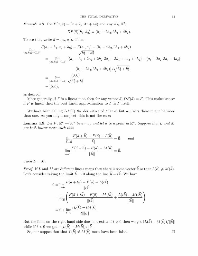
Example 4.8. For F (x, y) = (x+ 2y, 3x+ 4y) and any ~a ∈ R2,

DF (~a)(h1, h2) = (h1 + 2h2, 3h1 + 4h2).

To see this, write ~a = (a1, a2). Then,

lim(h1,h2)→(0,0)

F (a1 + h1, a2 + h2)− F (a1, a2)− (h1 + 2h2, 3h1 + 4h2)√h2

1 + h22

= lim(h1,h2)→(0,0)

[(a1 + h1 + 2a2 + 2h2, 3a1 + 3h1 + 4a2 + 4h2)− (a1 + 2a2, 3a1 + 4a2)

− (h1 + 2h2, 3h1 + 4h2)]/√h2

1 + h22

= lim(h1,h2)→(0,0)

(0, 0)√h2

1 + h22

= (0, 0),

as desired.More generally, if F is a linear map then for any vector ~a, DF (~a) = F . This makes sense:

if F is linear then the best linear approximation to F is F itself.

We have been calling DF (~a) the derivative of F at ~a, but a priori there might be morethan one. As you might suspect, this is not the case:

Lemma 4.9. Let F : Rn → Rm be a map and let ~a be a point in Rn. Suppose that L and Mare both linear maps such that

lim~h→~0

F (~a+ ~h)− F (~a)− L(~h)

‖~h‖= ~0 and

lim~h→~0

F (~a+ ~h)− F (~a)−M(~h)

‖~h‖= ~0.

Then L = M .

Proof. If L and M are different linear maps then there is some vector ~k so that L(~k) 6= M(~k).

Let’s consider taking the limit ~h→ 0 along the line ~h = t~k. We have

0 = limt→0

F (~a+ t~k)− F (~a)− L(t~k)

‖t~k‖

= limt→0

(F (~a+ t~k)− F (~a)−M(t~k)

‖t~k‖+L(t~k)−M(t~k)

‖t~k‖

)

= 0 + limt→0

tL(~k)− tM(~k)

|t|‖~k‖.

But the limit on the right hand side does not exist: if t > 0 then we get (L(~k)−M(~k))/‖~k‖while if t < 0 we get −(L(~k)−M(~k))/‖~k‖.

So, our supposition that L(~k) 6= M(~k) must have been false. �

14 ROBERT LIPSHITZ

4.3. The Jacobian matrix. Our definition of the total derivative should seem like a usefulone, and it generalizes the cases we already had, but some questions remain. Chief amongthem:

(1) How do you tell if a function Rn → Rm is differentiable? (And, are many of thefunctions one encounters differentiable?)

(2) How do you compute the total derivative of a function Rn → Rm?

The next theorem answers both questions; we will state it and then unpack it in someexamples.

Theorem 1. Suppose that F : Rn → Rm. Write F = (f1, . . . , fm), where fi : Rn → R. If forall i and j, ∂fi/∂xj is (defined and) continuous near ~a then F is differentiable at ~a, and thematrix for DF (~a) is given by

[DF (~a)] =

∂f1∂x1

∂f1∂x2

· · · ∂f1∂xn

∂f2∂x1

∂f2∂x2

· · · ∂f2∂xn

......

. . ....

∂fm

∂x1

∂fm

∂x2· · · ∂fm

∂xn

.

To avoid being sidetracked, we wont prove this theorem; its proof is similar to the proof ofStewart’s Theorem 8 in Section 14.4 (proved in Appendix F). (It is fairly easy to see that ifF is differentiable at ~a then [DF (~a)] has the specified form. Slightly harder is to show thatif all of the partial derivatives of the components of F are continuously differentiable thenF is differentiable.)

The matrix [DF (~a)] is called the total derivative matrix or Jacobian matrix of F at ~a.

Example 4.10. For the function F (x, y) = (x+ y2, x3 + 5y) from Example 4.7, the Jacobianmatrix at (1, 1) is

[DF ((1, 1))] =

(1 23 5

).

(Why?) This is, indeed, the matrix associated to the linear map from Example 4.7.

Example 4.11. Suppose F is the “turn cylindrical coordinates into rectangular coordinates”map from Example 1.8. Then

[DF (5, π/3, 0)] =

cos(θ) −r sin(θ) 0sin(θ) r cos(θ) 0

0 0 1

r=5,θ=π/3,z=0

=

1/2 −5√

3/2 0√3/2 5/2 00 0 1

.

Example 4.12. Problem. Suppose F : R2 → R2 is a differentiable map, F (1, 1) = (5, 8) and

[DF (1, 1)] =

(1 12 3

).

Estimate F (1.1, 1.2).Solution. Since F is differentiable,

F ((1, 1) + (.1, .2)) ≈ F (1, 1) +DF (1, 1)(.1, .2).


So,

F ((1, 1) + (.1, .2)) ≈(

58

)+

(1 12 3

)(.1.2

)=

(58

)+

(.3.8

)=

(5.38.8

).

Of course, we don’t know whether this is a good estimate or not: it depends whether(.1, .2) is a big or a small change for F .

Exercise 4.13. Compute the Jacobian matrices of the given maps at the given points:

(1) The map F : R2 → R2 defined by F (x, y) = (x2 + y3, xy) at (−1, 1).(2) The map F : R2 → R3 defined by F (x, y) = (xey, ye2x, x2 + y2) at (1, 1).(3) The map F : R3 → R defined by F (x, y, z) = x2 + y2 + z2 at (1, 2, 3).(4) The map G from Example 1.8,

G(ρ, θ, φ) = (ρ cos(θ) sin(φ), ρ sin(θ) sin(φ), ρ cos(φ)),

at the point (1, π/2, π/2).(5) The map G from Example 1.8,

G(ρ, θ, φ) = (ρ cos(θ) sin(φ), ρ sin(θ) sin(φ), ρ cos(φ)),

at the point (1, π/2, 0).

Exercise 4.14. Let F (r, θ) = (r cos(θ), r sin(θ)). (This map takes a vector in polar coordi-nates and rewrites it in rectangular coordinates.) Compute F (1, π/4) and [DF (1, π/4)]. Useyour computation to estimate F (1.01, π/4 + .02). Check your answer is reasonable using acalculator.

Exercise 4.15. Consider the map F : C→ C defined by F (z) = z2. We can identify C withR2 by identifying z = x+ iy in C with (x, y) in R2. Then, F is a map R2 → R2 given by

F (x, y) = (x2 − y2, 2xy).

Compute [DF ], [DF (1, 2)] and [DF (0, 0)].

Exercise 4.16. Consider the map F : C→ C given by F (z) = z3 + 2z. As in Exercise 4.15,we can view F as a map R2 → R2. Write F as a function F (x, y) and compute its Jacobianmatrix. Do you notice any symmetry in the matrix?

Exercise 4.17. Consider the map F : C → C given by F (z) = ez. As in Exercise 4.15, wecan view F as a map R2 → R2. Write F as a function F (x, y) and compute its Jacobianmatrix. (You will want to use Euler’s formula.) Do you notice any symmetry in the matrix?

5. Composition of linear maps and matrix multiplication

We showed in Lemma 2.8 that the composition of linear maps is a linear map. How doesthis relate to matrices? That is, if F : Rp → Rn and G : Rn → Rm are linear maps, how does[G ◦ F ] relate to [G] and [F ]? The answer is that [G ◦ F ] is the product of [G] and [F ].

Given a m× n and n× p matrices

A =

a1,1 a1,2 · · · a1,n

a2,1 a2,2 · · · a2,n...

.... . .

...am,1 am,2 · · · am,n

and B =

b1,1 b1,2 · · · b1,pb2,1 b2,2 · · · b2,p

......

. . ....

bn,1 bn,2 · · · bn,p

,

16 ROBERT LIPSHITZ

Figure 4. Multiplying matrices. Arrows indicate what your fingers shoulddo when computing three of the four entries.

the matrix product AB of A and B is the m× p matrix whose (i, j) entry2 is

ci,j = ai,1b1,j + ai,2b2,j + · · ·+ ai,nbn,j.

That is, to find the (i, j) entry of AB you run your left index finger across the ith row ofA and your right index finger down the jth column of B. Multiply the pairs of numbers yourfingers touch simultaneously and add the results. See Figure 4.

Example 5.1. A few example of matrix products:(2 30 4

)(−1 1−2 2

)=

(−2− 6 2 + 60− 8 0 + 8

)=

(−8 8−8 8

).

(1 2 34 5 6

)1 35 79 11

=

(1 + 10 + 27 3 + 14 + 334 + 25 + 54 12 + 35 + 66

)=

(38 5083 113

).

1 35 79 11

(1 2 34 5 6

)=

1 + 12 2 + 15 3 + 185 + 28 10 + 35 15 + 429 + 44 18 + 55 27 + 66

=

13 17 2133 45 5753 73 93

.

(By the way, I did in fact use my fingers when computing these products.)

Notice that the product of a matrix with a column vector as in Section 3 is a special caseof multiplication of two matrices.

2i.e., the entry in the ith row and jth column


Theorem 2. If F : Rp → Rn and G : Rn → Rm are linear maps then [G ◦ F ] = [G][F ].

Proof. We will only do the case m = n = p = 2; the general case is similar (but with indices).Write


G(x, y) = (ex+ fy, gx+ hy),

so on the one hand we have

G ◦ F (x, y) = ((ae+ cf)x+ (be+ df)y, (ag + ch)x+ (bg + dh)y),

[G ◦ F ] =

(ae+ cf be+ dfag + ch bg + dh

),

and on the other hand we have

[G] =

(e fg h

)[F ] =

(a bc d

)[G][F ] =

(ae+ cf be+ dfag + ch bg + dh

).

So, indeed, [G][F ] = [G ◦ F ], as desired. �

Corollary 5.2. The matrix product is associative. That is, if A is an m × n matrix, B isan n× p matrix and C is a p× r matrix then (AB)C = A(BC).

Proof. The matrix product corresponds to composition of functions, and composition offunctions is (obviously) associative.

(We could also verify this directly, by writing out all of the sums—but they becomepainfully complicated.) �

Notice that we have only defined the matrix product AB when the width of A is the sameas the height of B. If the width of A is not the same as the height of B then AB is simplynot defined. This corresponds to the fact that given maps F : Rq → Rp and G : Rn → Rm,G ◦ F only makes sense if p = n.

Example 5.3. The product (1 2 34 5 6

)(7 8 910 11 12

)is not defined: the first matrix has 3 columns but the second has only 2 rows. This corre-sponds to the fact that you can’t compose a map R3 → R2 with another map R3 → R2.

If you use your fingers, it’s obvious when a matrix product isn’t defined: one finger runsout of entries before the other.

Example 5.4. Even when the products in both orders are defined, matrix multiplication istypically non-commutative. For example:(

1 23 4

)(0 1−1 0

)=

(−2 1−4 3

)(

0 1−1 0

)(1 23 4

)=

(3 4−1 −2

).

18 ROBERT LIPSHITZ

(Actually, we had another example of this phenomenon in Example 5.1.)

Example 5.5. The dot product can be thought of as a special case of matrix multiplication.For example: (

1 2 3)2

24

= (2 + 4 + 12)

is the dot product of the vectors ~v = 〈1, 2, 3〉 and ~w = 〈2, 2, 4〉. The trick is to write the firstvector as a row vector and the second as a column vector.

Exercise 5.6. For each of the following, say whether the matrix product AB is defined, andif so compute it. Say also whether BA is defined, and if so compute it.

(1) A =

(3 21 0

), B =

(2 46 −2

).

(2) A =

(3 21 0

), B =

(5 3 12 2 4

).

(3) A = B =

0 1 00 0 11 0 0

(4) A =

1 22 33 4

, B =

1 1 10 1 10 0 1

(5) A =

(1 2 3

), B =

123

5.1. Matrix arithmetic. As something of an aside, we should mention that you can alsoadd matrices: if A and B are both n × m matrices then A + B is obtained by addingcorresponding entries of A and B. For example:(

1 2 34 5 6

)+

(2 2 33 4 4

)=

(3 4 67 9 10

).

There are two special (families of) matrices for matrix arithmetic. The n × n identitymatrix is the matrix with 1’s on it’s diagonal:

In×n =

1 0 0 · · · 00 1 0 · · · 00 0 1 · · · 0...

......

. . ....

0 0 0 · · · 1

.

The matrix In×n represents the identity map I : Rn → Rn given by I(~x) = ~x. (This takes alittle checking.)

The other special family are the m× n zero matrices, 0m×n, all of whose entries are 0:

0m×n =

0 0 · · · 0...

.... . .

...0 0 · · · 0

.


We might drop the subscripts n×n or m×n from In×n or 0m×n when the dimensions areeither obvious or irrelevant.

The properties of matrix arithmetic are summarized as follows.

Lemma 5.7. Suppose A, B, C and D are n×m, n×m, m×l and p×n matrices, respectively.Then:

(1) (Addition is commutative:) A+B = B + A.(2) (Additive identity:) 0n×m + A = A.(3) (Multiplicative identity:) In×nA = A = AIm×m.(4) (Multiplicative zero:) A0m×k = 0n×k. 0p×nA = 0p×m.(5) (Distributivity:) (A+B)C = AC +BC and D(A+B) = DA+DB.

(All of the properties are easy to check directly, and also follow from corresponding prop-erties of the arithmetic of linear maps.)

Exercise 5.8. Square the matrix A =

(0 1−1 0

), i.e., multiply A by itself. Explain geomet-

rically why the answer makes sense. (Hint: what linear map does A correspond to? Whathappens if you do that map twice?)

Exercise 5.9. Square the matrix B =

(2 −41 −2

). Does anything surprise you about the

answer?

Challenge Problem 5.10. Find a matrix A so that A 6= I but A3 = I. (Hint: thinkgeometrically.)

6. The chain rule for total derivatives

With the terminology we have developed, the chain rule is very succinct:

D(G ◦ F ) = (DG) ◦ (DF ).

More precisely:

Theorem 3. Let F : Rp → Rn and G : Rn → Rm be maps so that F is differentiable at ~aand G is differentiable at F (~a). Then

(6.1) D(G ◦ F )(~a) = DG(F (~a)) ◦DF (~a).

In particular, the Jacobian matrices satisfy

[D(G ◦ F )(~a)] = [DG(F (~a))][DF (~a)].

We will prove the theorem a little later. First, some examples and remarks.Notice that Equation (6.1) looks a lot like the chain rule for functions of one variable,

(g ◦ f)′(x) = f ′(x)g′(f(x)). Of course, the one-variable chain rule is a (very) special caseof Theorem 3, so this isn’t a total surprise. But it’s nice that we have phrased things, andchosen notation, so that the similarity manifests itself.

Example 6.2. Question. Let F (x, y) = (x + y2, x3 + 5y) and G(x, y) = (y2, x2). Compute[D(G ◦ F )] at (1, 1).

Solution. We already computed in Example 4.10 that

[DF (1, 1)] =

(1 23 5

).

20 ROBERT LIPSHITZ

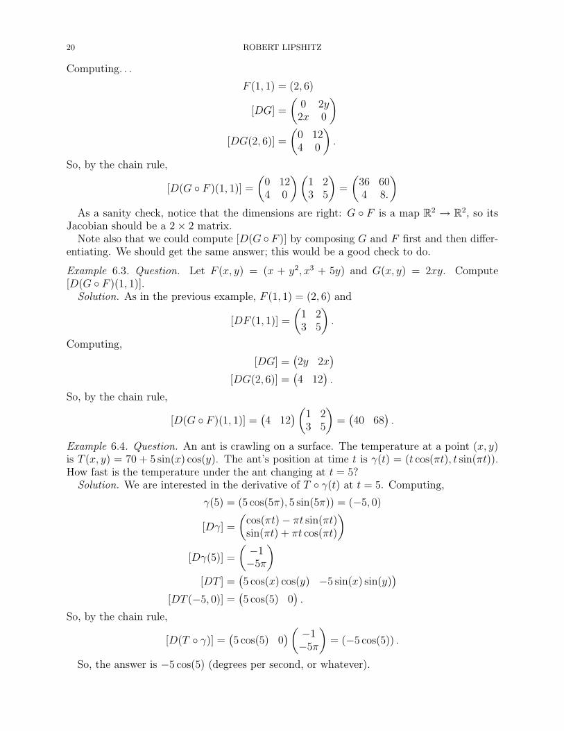
Computing. . .

F (1, 1) = (2, 6)

[DG] =

(0 2y

2x 0

)[DG(2, 6)] =

(0 124 0

).

So, by the chain rule,

[D(G ◦ F )(1, 1)] =

(0 124 0

)(1 23 5

)=

(36 604 8.

)As a sanity check, notice that the dimensions are right: G ◦ F is a map R2 → R2, so its

Jacobian should be a 2× 2 matrix.Note also that we could compute [D(G ◦ F )] by composing G and F first and then differ-

entiating. We should get the same answer; this would be a good check to do.

Example 6.3. Question. Let F (x, y) = (x + y2, x3 + 5y) and G(x, y) = 2xy. Compute[D(G ◦ F )(1, 1)].

Solution. As in the previous example, F (1, 1) = (2, 6) and

[DF (1, 1)] =

(1 23 5

).

Computing,

[DG] =(2y 2x

)[DG(2, 6)] =

(4 12

).


[D(G ◦ F )(1, 1)] =(4 12

)(1 23 5

)=(40 68

).

Example 6.4. Question. An ant is crawling on a surface. The temperature at a point (x, y)is T (x, y) = 70 + 5 sin(x) cos(y). The ant’s position at time t is γ(t) = (t cos(πt), t sin(πt)).How fast is the temperature under the ant changing at t = 5?

Solution. We are interested in the derivative of T ◦ γ(t) at t = 5. Computing,

γ(5) = (5 cos(5π), 5 sin(5π)) = (−5, 0)

[Dγ] =

(cos(πt)− πt sin(πt)sin(πt) + πt cos(πt)

)[Dγ(5)] =

(−1−5π

)[DT ] =

(5 cos(x) cos(y) −5 sin(x) sin(y)

)[DT (−5, 0)] =

(5 cos(5) 0

).


[D(T ◦ γ)] =(5 cos(5) 0

)( −1−5π

)= (−5 cos(5)) .

So, the answer is −5 cos(5) (degrees per second, or whatever).


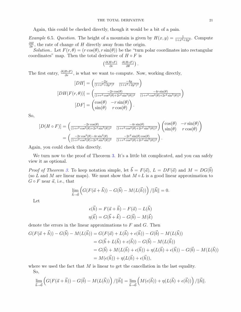
Again, this could be checked directly, though it would be a bit of a pain.

Example 6.5. Question. The height of a mountain is given by H(x, y) = 11+x2+2y2

. Compute∂H∂r

, the rate of change of H directly away from the origin.Solution.. Let F (r, θ) = (r cos(θ), r sin(θ)) be the “turn polar coordinates into rectangular

coordinates” map. Then the total derivative of H ◦ F is(∂(H◦F )∂r

∂(H◦F )∂θ

).

The first entry, ∂(H◦F )∂r

, is what we want to compute. Now, working directly,

[DH] =(

−2x(1+x2+2y2)2

−4y(1+x2+2y2)2

)[DH(F (r, θ))] =

(−2r cos(θ)

(1+r2 cos2(θ)+2r2 sin2(θ))2−4r sin(θ)

(1+r2 cos2(θ)+2r2 sin2(θ))2

)[DF ] =

(cos(θ) −r sin(θ)sin(θ) r cos(θ)

).

So,

[D(H ◦ F )] =(

−2r cos(θ)

(1+r2 cos2(θ)+2r2 sin2(θ))2−4r sin(θ)

(1+r2 cos2(θ)+2r2 sin2(θ))2

)(cos(θ) −r sin(θ)sin(θ) r cos(θ)

)=(

−2r cos2(θ)−4r sin2(θ)

(1+r2 cos2(θ)+2r2 sin2(θ))2−2r2 sin(θ) cos(θ)

(1+r2 cos2(θ)+2r2 sin2(θ))2

).

Again, you could check this directly.

We turn now to the proof of Theorem 3. It’s a little bit complicated, and you can safelyview it as optional.

Proof of Theorem 3. To keep notation simple, let ~b = F (~a), L = DF (~a) and M = DG(~b)(so L and M are linear maps). We must show that M ◦L is a good linear approximation toG ◦ F near ~a, i.e., that

lim~h→~0

(G(F (~a+ ~h))−G(~b)−M(L(~h))

)/‖~h‖ = 0.

Let

ε(~h) = F (~a+ ~h)− F (~a)− L(~h)

η(~k) = G(~b+ ~k)−G(~b)−M(~k)

denote the errors in the linear approximations to F and G. Then

G(F (~a+ ~h))−G(~b)−M(L(~h)) = G(F (~a) + L(~h) + ε(~h))−G(~b)−M(L(~h))

= G(~b+ L(~h) + ε(~h))−G(~b)−M(L(~h))

= G(~b) +M(L(~h) + ε(~h)) + η(L(~h) + ε(~h))−G(~b)−M(L(~h))

= M(ε(~h)) + η(L(~h) + ε(~h)),

where we used the fact that M is linear to get the cancellation in the last equality.So,

lim~h→~0

(G(F (~a+ ~h))−G(~b)−M(L(~h))

)/‖~h‖ = lim

~h→~0

(M(ε(~h)) + η(L(~h) + ε(~h))

)/‖~h‖.

22 ROBERT LIPSHITZ

Thus, it’s enough to show that

lim~h→~0

M(ε(~h))

‖~h‖= 0 and

lim~h→~0

η(L(~h) + ε(~h))

‖~h‖= 0.

For the first, notice that there is some constant C, depending on M , so that for any vector~v, ‖M(~v)‖ ≤ C‖~v‖. So, ∥∥∥∥∥M(ε(~h))

‖~h‖

∥∥∥∥∥ ≤ C

∥∥∥∥∥ε(~h)

‖~h‖

∥∥∥∥∥→ 0,

as desired.For the second, if we let ~k = L(~h) + ε(~h) then there is a constant D so that for any ~h,

‖~h‖ ≥ D‖~k‖. Moreover, as ~h→ 0, ~k → 0 as well. So, for ~h so that ~k 6= 0,∥∥∥∥∥η(L(~h) + ε(~h))

‖~h‖

∥∥∥∥∥ ≤ 1

D

∥∥∥∥∥η(~k)

‖~k‖

∥∥∥∥∥→ 0

as ~k → 0. For ~h so that ~k = ~0, η(L(~h)+ε(~h))

‖~h‖is exactly zero. So, as ~h→ 0, η(L(~h)+ε(~h))/‖~h‖ →

0, as desired.This proves the result. �

Exercise 6.6. Let F (x, y) = (x2y, xy2) and G(x, y) = (x/y, y/x). Use the chain rule tocompute [D(G◦F )(1, 2)]. Check your answer by composing G and F and then differentiating.

6.1. Comparison with the treatment in Stewart’s Calculus. We already saw severalspecial cases of Theorem 3, in a somewhat disguised form, earlier in the semester. Thefollowing is quoted from Stewart, Section 14.5 (box 4):

Theorem 4. Suppose u is a differentiable function of n variables x1, x2, . . . , xn and each xjis a differentiable function of m variables t1, t2, . . . , tm. Then u is a function of t1, t2, . . . , tmand

∂u

∂ti=

∂u

∂x1

∂x1

∂ti+

∂u

∂x2

∂x2

∂ti+ · · ·+ ∂u

∂xn

∂xn∂ti

for each i = 1, 2, . . . ,m.

As a special case, he noted that if z is a function of x and y and x and y are functions ofs and t then

∂z

∂s=∂z

∂x

∂x

∂s+∂z

∂y

∂y

∂sand

∂z

∂t=∂z

∂x

∂x

∂t+∂z

∂y

∂y

∂t.

Let’s see how the special case fits into our framework, and then how Stewart’s “general”case does.

In the special case, we have z = z(x, y). Let F (s, t) = (x(s, t), y(s, t)). We are interested

in the partial derivatives of z ◦ F ; for example, ∂z∂s

really means ∂(z◦F )∂s

. On the one hand,

[D(z ◦ F )] =(∂(z◦F )∂s

∂(z◦F )∂t

).


On the other hand,

[Dz] =(∂z∂x

∂z∂y

)[DF ] =

(∂x∂s

∂x∂t

∂y∂s

∂y∂t

)so

[Dz][DF ] =(∂z∂x

∂x∂s

+ ∂z∂y

∂y∂s

∂z∂x

∂x∂t

+ ∂z∂y

∂y∂t

).

By the chain rule, [D(z ◦ F )] = [Dz] ◦ [DF ], so

∂(z ◦ F )

∂s=∂z

∂x

∂x

∂s+∂z

∂y

∂y

∂s

∂(z ◦ F )

∂t=∂z

∂x

∂x

∂t+∂z

∂y

∂y

∂t,

exactly as in Stewart.The general case is similar. Let F (t1, . . . , tm) = (x1(t1, . . . , tm), . . . , xn(t1, . . . , tm)). Then,

[Du] =(∂u∂x1

· · · ∂u∂xn

)[DF ] =

∂x1

∂t1· · · ∂x1

∂tm...

. . ....

∂xn

∂t1· · · ∂xn

∂tm

.

So,[Du][DF ] =

(∂u∂x1

∂x1

∂t1+ · · ·+ ∂u

∂xn

∂xn

∂t1· · · ∂u

∂x1

∂x1

∂tm+ · · ·+ ∂u

∂xn

∂xn

∂tm

).

Equating this with

D(u ◦ F ) =(∂(u◦F )∂t1

· · · ∂(u◦x)∂tm

)gives the “general” form of the chain rule from Stewart.

Exercise 6.7. Stewart also stated a special case of the chain rule when z = z(x, y) andx = x(t), y = y(t). Explain how this special case follows from Theorem 3.

Department of Mathematics, Columbia University, New York, NY 10027E-mail address: [email protected]

linear maps, the total derivative and the chain rule

Documents