linear one-step processes with artiﬁcial boundariesfbssaz/articles/azaele_jsp06.pdf ·...

Journal of Statistical Physics, Vol. 125, No. 2, October 2006 ( C© 2006 )DOI: 10.1007/s10955-006-9158-z

Linear One-Step Processes with Artificial Boundaries

Sandro Azaele,1 Igor Volkov,2,3 Jayanth R. Banavar,2 and Amos Maritan4

Received March 31, 2006; accepted June 8, 2006Published Online: September 13, 2006

An artificial absorbing boundary is introduced in a linear birth and death stochasticprocess in order to understand the long time behavior of an ecological community. Thesolution is obtained by means of a spectral resolution of the probability distribution. Amore general linear process with a coefficient of arbitrary strength near the boundaryboth with absorbing and with reflecting boundary conditions is also studied.

KEY WORDS: One-step stochastic processes, spectral resolution, ecological commu-nity, artificial boundaries, neutral theory of biodiversity

1. INTRODUCTION

Birth and death stochastic processes have been studied in depth and applied toa wide variety of physical, chemical and biological systems (see Refs. 1 and 2).When the master equation governing these processes involves a boundary, onecan solve it with artificial or natural boundary conditions, namely with or withoutaltering the behavior of the birth and death coefficients near the edge (see Ref. 1).In other words, a master equation has an artificial boundary when there exists atleast one site that is described by a special equation, which does not include theanalytical expression of bn (birth rate) or dn (death rate) that governs the othersites.

For example, a quantized harmonic oscillator interacting with a radiationfield can be described by a one-step master equation with bn = b(n + 1) anddn = dn, which drives the probability per unit time for a jump from n to n + 1

1 Dipartimento di Fisica G. Galilei, Universita di Padova, via Marzolo 8, 35131 Padova, Italy.2 Department of Physics, The Pennsylvania State University, 104 Davey Laboratory, University Park,

Pennsylvania 16802, USA.3 Center for Infectious Disease Dynamics, The Pennsylvania State University, 208 Mueller Laboratory,

University Park, Pennsylvania 16802, USA.4 Dipartimento di Fisica G. Galilei Universita di Padova and INFM via Marzolo 8, 35131 Padova, Italy.

495

0022-4715/06/1000-0495/0 C© 2006 Springer Science+Business Media, Inc.

496 Azaele, Volkov, Banavar, and Maritan

and from n to n − 1, respectively. Without changing the value of the coefficientsat the boundary n = 0, it is possible to reach the well-known reflecting stationarysolution Pn ∝ (b/d)n . In contrast, other phenomena described by bn = bn anddn = dn are naturally absorbing at n = 0 and the trivial steady-state solution isPn = δn,0 (see Refs. 1 and 2).

Bounded random walks with reflecting and absorbing boundary conditionshave been analyzed with coefficients of arbitrary strength at n = 0 by involvingsome suitable equations at the boundary. One-step processes with these artifi-cial boundaries have been extensively used in the study of many physical effectslike evaporation of a gas through a surface, ionic currents through cell mem-branes, defect diffusion in crystals, chemical reactions and queuing problems (seeRefs. 3–5).

Linear birth and death processes (bn = bn + b, dn = dn + d) have beenstudied by Karlin and McGregor Ref. 6 by using the left eigenvectors of theinfinitesimal matrix generating the process. Their approach relies decisively onthe knowledge of the elaborate structure of general birth and death processes asdeveloped in Refs. 7 and 8. They demonstrated that a birth and death process isintimately linked to a Stieltjes moment problem. This connection enabled them toachieve the conditions for the existence and uniqueness of the spectral resolutionof the probability distribution (see Ref. 9 for further developments along theselines).

In this paper we present a more straightforward and self-contained analysis ofboth the discrete spectrum and the (left and right) eigenvectors for linear one-stepprocesses with artificial boundaries. Our approach relies only on some propertiesof the solution of the Laplace transformed equation of the process. Furthermorethe spectral resolution of a more general problem (which includes both absorbingand reflecting boundaries) can also be obtained within our method.

In the last few years linear stochastic processes with artificial boundarieshave been applied to the time evolution of ecosystems, mostly within the neu-tral theory of biodiversity (see Refs. 10–12). This theory provides a frameworkwhich accounts for the distribution of the relative species abundance both for themetacommunity and the local community (see Refs. 11 and 13).

The neutrality hypothesis is a symmetry assumption at the individual level. Itpostulates that all species obey the same interaction rules on a per capita basis (seeRef. 10). This oversimplified hypothesis, that resembles the ideal gas assumptionin statistical physics, is equivalent to the assumption that the dynamics of thespecies is due to the similarity rather than differences between the species.

A slightly modified theory (see Ref. 12), which incorporates density depen-dence, assumes a rare species advantage by introducing a birth rate bn = bn + band a death rate dn = dn + d for an arbitrary species with n individuals. Since aspecies disappears when its last individual dies, one should solve the master equa-tion, which drives the population dynamics, with an artificial absorbing boundary

Linear One-Step Processes with Artificial Boundaries 497

at n = 0. We wish to stress that, even though in this case the stationary solutionis trivial, owing to Frobenius’ theorem (see Ref. 14), the first eigenfunction of thespectral resolution of pn(t) can be interpreted as the population distribution of agiven species on time scales µ−1

1 , where µ1 is the first eigenvalue. The continuumformulation with a Fokker–Planck equation for a less general diffusion problemwas pointed out by Feller many years ago (see Ref. 15 he stressed the importanceof such singular diffusion equations for the theory of stochastic processes and thetheory of semigroups as well.

The structure of the paper is as follows: In Sec. 2 we will derive a solutionfor the generating function for the master equation with absorbing boundaryconditions; In Sec. 3 we will find eigenvalues and eigenfunctions for the probabilitydistribution function; and in Sec. 4 we will consider a solution for the generalizedcase of the boundary conditions.

2. ABSORBING CASE

In this section we present the calculations for the absorbing case. Whendealing with absorbing boundaries, one should be aware of the existence anduniqueness of the solutions of the birth-death master equation. In fact, the nonconservation of the total probability may cause a dependence on initial conditionsof the stationary distribution. Yet if the process is linear, it is possible to proveboth the existence and the uniqueness of the solution (see Ref. 16).

The linearity of the process also ensures that the spectrum is discrete withnon negative eigenvalues (see below) when b �= d, instead it is continuous andunbounded when b = d. If the process is a left-bounded random walk (symmetricor asymmetric), then the spectrum is continuous and bounded (see Refs. 1, 4 and16).

Let us suppose that the time evolution of a population of a given speciesis governed by the following birth-death master equation (n = 0, 1, 2, . . .) withabsorbing boundary conditions (abc) at n = 0

∂pn(t)

∂t= bn−1 pn−1(t) + dn+1 pn+1(t) − (bn + dn)pn(t) (1)

where the birth and death rates are given by

b0 = 0 and bn = bn + b for n > 0d0 = 0 and dn = dn + d for n > 0.

(2)

To avoid ambiguities, during the calculations we shall suppose that b, d > 0 andb �= d, but b and d could possibly take negative real values. Notice that if we knowp1(t) then we also know p0(t), because p0(t) = d1 p1(t) (we set b−1 ≡ 0).

We now seek an expansion in (right) eigenvectors of the solution of Eq. (1)in the abc case (2) with a specified initial condition pn(0). For our purposes, we


define the following generating function

F(z, t) = zε

∞∑

n=1

pn(t)zn (3)

for 0 < z < 1 and 0 < t < ∞, where the real parameter ε will be defined later.Using this definition we can transform the previous problem into an inho-

mogeneous first order p.d.e. for F(z, t) with suitable initial conditions and choosethe parameter ε to obtain a bounded solution. The p.d.e. is of the first order due tothe linearity of the birth and death coefficients and it is inhomogeneous becauseof the barrier at n = 0. Carrying out the calculations, we get

∂ F(z, t)

∂t= A(z)

∂ F(z, t)

∂z+ A(z)F(z, t) + f (z, t) (4)

where

A(z) = (1 − z)(d − bz)

A(z) = (1 − z)bd − db

d(5)

f (z, t) = −d1zdd p1(t)

and p1(t) is the unknown probability of having just one individual at time t . Sincen is not allowed to take negative values, we have fixed ε = d/d to remove thesingularity at z = 0. The initial condition for F(z, t) is

F(z, 0) = g(z) (6)

where g(z) is a sufficiently smooth function with g(1) = 1. This kind of inhomo-geneous p.d.e. may be readily solved with the aid of the Duhamel’s principle (seeRefs. 17–19).

In fact, let F0(z, t) be the solution of the homogeneous p.d.e.⎧⎪⎪⎨

⎪⎪⎩

∂ F0(z, t)

∂t= A(z)

∂ F0(z, t)

∂z+ A(z)F0(z, t)

F0(z, 0) = g(z)

(7)

Moreover, let F1(z, t, τ ) be the solution of the following homogeneous p.d.e.⎧⎪⎪⎨

⎪⎪⎩

∂ F1(z, t, τ )

∂t= A(z)

∂ F1(z, t, τ )

∂z+ A(z)F1(z, t, τ )

F1(z, t, t) = f (z, t) for τ = t

(8)


where τ is a fixed parameter that simply labels the solution and A(z), A(z), f (z, t)and g(z) are defined as in (5) and (6). Thus if we know the solutions of the initialvalue problems (7) and (8) then we also know the solution of the inhomogeneousp.d.e. (4) with the correct initial values (6), i.e.

F(z, t) = F0(z, t) +∫ t

0F1(z, t, τ ) dτ (9)

For the total probability W (t) = ∑∞n=1 pn(t) we have

∂W

∂t= −(d + d)p1(t) = ∂ F(1, t)

∂t(10)

and hence there is a reflecting boundary at n = 1 when d/d = −1 and an ab-sorbing one at n = 0 when d/d > −1 (the case d/d < −1 describes a neg-ative effective death rate which we are not interested in.) For the probabilityp0(t) = 1 − ∑∞

n=1 pn(t) of the population becoming extinct at time t one gets

p0(t) = − f (1, t) = (d + d)p1(t) (11)

therefore the inhomogeneous term of (4) takes into account the flux towards n = 0.The initial value problems (7) and (8) are readily solved by means of the

familiar method of characteristics. After lengthy but standard calculations, onefinally achieves the explicit form of the solution (9)

F(z, t) =(

d − bz − b(1 − z)e(b−d)t

d − b

) dd − b

b

g

(d − bz − d(1 − z)e(b−d)t

d − bz − b(1 − z)e(b−d)t

)

− d + d

(d − b)dd − b

b

∫ t

0

[d − bz − d(1 − z)e(b−d)(t−τ )

] dd

[d − bz − b(1 − z)e(b−d)(t−τ )

] bb

p1(τ )d τ (12)

Notice that the integrand in (12) converges uniformly with respect to τ and onecan take a derivative with respect to z directly.

Note moreover that the solution naturally splits into two parts: the first oneis important only at short times and close to the initial condition g(z), the secondone dominates at long time scales and close to the left boundary at n = 0 if b < dor close to both boundaries (zero and infinity) if b > d. Obviously this is not at alla complete solution to our problem, because we do not know p1(t) yet. Anywaywe can readily obtain an equation for p1(t) by requiring that it is constructed soas to satisfy the condition

limz→0+

F(z, t) = 0 (13)

that is always true in the absorbing case (i.e. d/d > −1 and x ≡ b/d, 0 < x < 1from now on, for avoiding the possibility of demographic explosion). Notice that


limz→1− F(z, t) = 1 − p0(t) only yields the identity p0(t) = (d + d)∫ t

0 p1(τ )dτ .Conversely the limit (13) immediately gives the following integral equation forp1(t)

d1

∫ t

0

[1 − e(b−d)(t−τ )

] dd

[1 − xe(b−d)(t−τ )

] bb

p1(τ ) dτ =[1 − e(b−d)t

] dd +N

[1 − xe(b−d)t

] bb +N

(14)

where we have chosen the initial condition pn(0) = δn,N , which implies g(z) =z

dd +N due to the definition of the generating function in (3) and (6). The Eq. in

(14) is a Volterra equation (see Ref. 20) whose kernel, having no singularities for0 < x < 1, is analytic and only depends on t − τ . Therefore the unique solutionis analytic and may be found by means of the familiar Laplace transform.

Thus by taking the Laplace transform of the integral Eq. (14) and using theconvolution theorem (see Ref. 18), one achieves for s > 0

L{p1(t)} ≡∫ ∞

0p1(t)e−st dt ≡ p1(s) = 1

d1

L{χ (t)}L{κ(t)} (15)

where

κ(t) ≡[1 − e(b−d)t

] dd

[1 − xe(b−d)t

] bb

, χ (t) ≡[1 − e(b−d)t

] dd +N

[1 − xe(b−d)t

] bb +N

(16)

Now with the change of variable

e(b−d)t = 1 − z

1 − xz(17)

the Laplace transform κ(s) of the kernel κ(t) may be written as

κ(s) = K∫ 1

0z

dd (1 − z)

sd−b −1(1 − xz)

bb − d

d − sd−b −1dz (18)

where K = (1−x)dd − b

b

d . As s > 0 and x < 1 we can use the integral representation ofthe standard hypergeometric function (see Refs. 21 and 22), then we may rewritethe previous equation as

κ(s) = K�(β) �(γs − β)

�(γs)F(αs, β, γs ; x) (19)


with the following definitions⎧⎪⎪⎪⎪⎪⎨

⎪⎪⎪⎪⎪⎩

αs ≡ s

d − b+ 1 + d

d− b

b

β ≡ 1 + d

d

γs ≡ s

d − b+ 1 + d

d

(20)

where �(z) and F(α, β, γ ; x) are the gamma function and the standard hyper-geometric function respectively (see Refs. 21 and 22). Note that, as x is a fixedparameter smaller than one, in Eq. (19) the condition s > 0 can be dropped,because in the hypergeometric function the variable s appears only inside its co-efficients. Therefore Eq. (19) may be regarded as the analytic continuation of theLaplace transform κ(s) inside the complex plane and then s may assume negativevalues as well. Furthermore the function (19) is an entire function of s by virtueof the denominator �(γs), that removes the simple poles of F(α, β, γ ; x). In fact,there are also the simple poles sn = −n(d − b), owing to the gamma function, butthese will be dropped later.

The preceding integral representation of the hypergeometric function enableus to carry out the analytic continuation of L{χ (t)} as well, removing the restric-tions on the variable s. Finally, one gets for L{χ (t)} the following expression

K�(β + N ) �(γs − β)

�(γs + N )F(αs, β + N , γs + N ; x) (21)

The Eqs. (19) and (21) lead to

p1(s) = �(β + N )

d1�(β)

�(γs)

�(γs + N )

F(αs, β + N , γs + N ; x)

F(αs, β, γs ; x)(22)

and is the solution in (15). It is worth noting that the integral equations of the form(14), i.e.

∫ t

0N (t − τ )p1(τ ) dτ = I(t) (23)

with I(0) = 0 can be solved with the aid of the residue theorem. In fact, by meansof the convolution theorem, we find

p1(s) = I(s)

N (s)(24)

where I(s) and N (s) are the Laplace transforms of I(t) and N (t) respectively.If N (s) and I(s) are analytic functions such that N (s) has simple, isolated zerosat s = −µ� but ∂sN (−µ�) �= 0 and I(−µ�) �= 0 for any � (see below for the


meaning of µ�), then the solution can be written down as

p1(t) =∑

�

I(−µ�)

∂sN (−µ�)e−µ�t (25)

Therefore by means of (22) and if one knows the µ�’s, this produces a completesolution to the problem of finding the generating function in (12).

3. EIGENFUNCTIONS AND EIGENVALUES

IN THE ABSORBING CASE

3.1. Eigenfunctions

When b �= d one can prove that linear one-step processes have a discretespectrum with only real non-negative eigenvalues (see Ref. 16). We now seek theprobability distribution in an eigenfunction expansion of the form

pn(t) = P statn +

∞∑

�=1

c�φ�ne−µ�t for n = 0, 1, 2, . . . (26)

The (right) eigenfunctions are φ�n (with φ0

n = P statn , c0 = 1) and the eigenvalues

are such that

µ0 = 0 < µ1 < µ2 < . . . < µ� < . . . for � ∈ N (27)

In this form the eigenvalues µ� are always non-negative and they are the sameboth for right and left eigenfunctions. General orthogonality and completenessproperties of birth and death eigenfunctions have been firstly studied by Ledermannand Reuter Ref. 16 and secondly by Karlin and McGregor Ref. 7 and 8. When thespectrum is discrete, it is known that in the linear case the right eigenvectors are theMeixner or the associated Meixner polynomials (see Ref. 9). These polynomialsare orthogonal with respect to a discrete measure (see Appendix B, Refs. 23 and24). Now we obtain these polynomials in a more direct way.

The previous definitions, the following relations hold in the abc case

F(z, t) = zε

∞∑

n=1

pn(t)zn =∞∑

�=1

c�φ�(z)e−µ�t

φ�(z) ≡ zε

∞∑

n=1

φ�nzn for � = 1, 2, . . . (28)

If we carry out the Laplace transform of pn(t) and F(z, t), we get (n > 0)

pn(s) =∞∑

�=1

c�φ�n

s + µ�


F(z, s) =∞∑

�=1

c�φ�(z)

s + µ�

(29)

It should be noted that F(z, s) is well defined with respect to the variable s inthe whole complex plane, and thus this equation may be defined as the analyticcontinuation of the Laplace transform (15) as carried out for Eq. (19).

Moreover, for our purposes it is important to stress that the (simple) poles ofF(z, s) (or p1(s) as well) are the eigenvalues of the expansion (26) and the �-thresidue of F(z, s) is proportional to the generating function for the �-th eigen-function. Indeed if Cµ�

is a closed simple path that encircles only the singularitys = −µ� then, by means of the residue theorem, it turns out

∮

Cµ�

F(z, s) ds = 2π i c�φ�(z). (30)

One finds that

φ�(z) ∝ lims→−µ�

(s + µ�)F(z, s). (31)

Owing to the equation p0(t) = d1∫ t

0 p1(τ )dτ and to the expression in (26)for n = 1, one readily gets

p0(t) = 1 − d1

∞∑

�=1

c�

µ�

φ�1e−µ�t (32)

because limt→∞ p0(t) = 0, whereas p0(t) = 1 + ∑∞�=1 c�φ

�0e−µ�t by definition in

(26). Hence one obtains

φ00 = 1 and φ�

0 = − d1

µ�

φ�1 for � = 1, 2, . . . (33)

In order to achieve a general expression for φ�n , we shall exploit the relation (31).

When carrying out the Laplace transform it is possible to follow two differentroutes. Either one finds the solution of the Laplace transformed Eq. (4) or onecarries out directly the Laplace transform of the solution (12). If the integral∫ ∞

0 F(z, t)e−st dt converges uniformly with regard to z and s in their respectivedomains, then the two ways would be equivalent. But this is not the case. In fact,it is possible to see that in general ∂zL{F(z, t)} �= L{∂z F(z, t)}, which breaks theuniform convergence of the previous integral (see Ref. 25).

Laplace transforming the Eq. (4), one can see that the solution F(z, s) hasthe form

F(z, s) = C(z, s) + D(z, s) p1(s) (34)


where

C(z, s) = − 1

dzβ+N (1 − z)β−γs (1 − xz)αs−1

×∫ 1

0dt tβ−1+N (1 − zt)γs−β−1(1 − xzt)−αs

D(z, s) = βzβ(1 − z)β−γs (1 − xz)αs−1

×∫ 1

0dt tβ−1(1 − zt)γs−β−1(1 − xzt)−αs (35)

But the Laplace transform of the solution (12) has the form

F(z, s) = C(z, s) + D(z, s) p1(s) (36)

where

C(z, s) = C(z, s) + 1

d(1 − z)β−γs (1 − xz)αs−1

× �(β + N ) �(γs − β)

�(γs + N )F(αs, β + N , γs + N ; x)

D(z, s) = D(z, s) − β(1 − z)β−γs (1 − xz)αs−1

× �(β) �(γs − β)

�(γs)F(αs, β, γs ; x) . (37)

It is worth noting that when F(αs, β, γs ; x) = 0 (as a function of s), one obtainsin general D(z,−µ�) = D(z,−µ�) but C(z,−µ�) �= C(z,−µ�), regardless of z.As it will be pointed out below, this ensures us that if s = −µ�, the failure of theuniform convergence affects only the part of (12) involving the initial conditions.Therefore the two preceding routes are equivalent in order to obtain eigenvaluesand eigenvectors, even though the correct generating function of the process to beused is (12).

The functions C(z, s) and D(z, s) do not have any poles (see Appendix A)for s = −µ� (note that if C(z, s) had any poles for s = −µ� then the eigenvalueswould depend on the initial conditions). Thus we find the generating function ofthe right eigenfunctions, which is that of the associated Meixner polynomials (asin Ref. 9)

φ�(z) ∝ D(z,−µ�) (38)

Now one may succeed in drawing out the eigenfunctions φ�n by expanding

D(z,−µ�) in powers of z. Such an expansion is readily accomplished by mak-ing use of a formula which is proven in Appendix B. The calculations (madein Appendix A) lead to the eigenfunctions φ�

n (for n, � = 1, 2, . . .), which are


proportional to

n−1∑

k=0

1

k + βP (� , σ�−1−k)

k (2x − 1)P (−� , n−1−k−σ�)n−1−k (2x − 1) (39)

where P (α,β)n (z) are the Jacobi’s polynomials (see Refs. 9, 21 and 26) and

� = 1 + d

d− b

b

σ� = −µ�

d − b(40)

Thus, if we are given the eigenvalues µ� then we have solved the problem offinding the time dependent solution in (26) for the abc case.

The previous considerations can be put forward again for the left eigenvectors.After setting ε = b/b − 1 > −1, it is possible to see that the solution of the Laplacetransformed equation (using now left eigenvectors) has a form similar to (34), thatis

G(z, s) = C(z, s) + D(z, s)q1(s) (41)

but in this case we have

D(z, s) = βzβ(1 − z)β−γs

(1 − z

x

)αs−1

×∫ 1

0d t t β−1(1 − zt)γs−β−1

(1 − z

xt)−αs

(42)

where⎧⎪⎪⎪⎪⎪⎨

⎪⎪⎪⎪⎪⎩

αs ≡ − s

d − b− d

d+ b

b

β ≡ b

b

γs ≡ − s

d − b+ 1 + b

b

(43)

Thus the generating function of the left eigenfunctions is φ�(z) ∝ D(z,−µ�) andone may succeed in drawing out the left eigenfunctions φ�

n by expanding D(z,−µ�)in powers of z as just seen. The relations between right and left coefficients are

⎧⎨

⎩

αs = 1 − αs

β = γs − αs

γs = 1 − αs + β

(44)


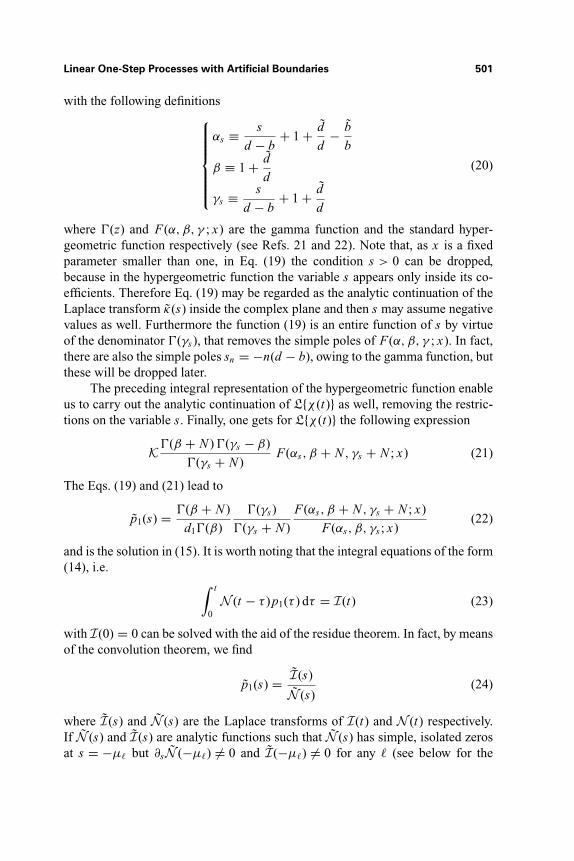
Fig. 1. The upper figure shows the first two roots of F(αs , β, γs ; x) as a function of s when b = 1, d =2, b = 4, d = 3. For the same parameters the lower figure shows the first five roots.

3.2. Eigenvalues

When b �= 0 it is easy to show that the only poles of p1(s) are the solutionsof the equation

F(αs, β, γs ; x) = 0 (45)

as a function of s. Otherwise, if b = 0, the only poles of p1(s) are those of �(γs).In fact, when b �= 0 the function F(αs, β, γs ; x) does depend on s and the

product

1

�(γ )F(α, β, γ ; x) (46)

is an entire function of α, β and γ , for fixed x (see Ref. 22). Furthermore,when N > 0 there are no zeros of F(αs, β + N , γs + N ; x) that overlap thoseof F(αs, β, γs ; x), otherwise the eigenvalues would depend on the initial condi-tions. On the contrary, if b = 0 then F(αs, β, γs ; x) does not depend on s and wehave only the poles of �(γs).

It is not possible to give an analytical expression for the eigenvalues in fullgenerality (Fig. 1 shows the plot of F(αs, β, γs ; x) as a function of s for arbitrary


values of b, d, b, d). Yet when x → 1, it is possible to get a simpler expressionfor µ1. If the parameters of the standard hypergeometric function F(a, b, c; z) aresuch that �(c − a − b) > 0, then it is possible to calculate the value F(a, b, c; 1)(see Ref. 22):

limz→1−

F(a, b, c; z) = �(c)�(c − a − b)

�(c − a)�(c − b)(47)

where �(z) is the gamma function. If the first eigenvalue is much less than 1 inunits of d − b, then |s/(d − b)| 1 and we can write

µ1 = 2(d − b)

∣∣∣∣∣∂ς=0 F(αs, β, γs ; 1)

∂2ς=0 F(αs, β, γs ; 1)

∣∣∣∣∣ (48)

where ς = s/(d − b). Thus, when b > βb it is possible to write down at theleading order

µ1 = (d − b)1

|�(β) + γ | (49)

where �(z) is the logarithmic derivative of the gamma function (see Ref. 22) andγ = 0.577 . . . is the Euler’s constant. In order to get µ1 1, one also needs that1 β < b/b.

When the parameter b is zero, the function F(αs, β, γs ; x) does not dependon s because αs = γs ; in this case F(αs, β, αs ; x) = (1 − x)−β . As the poles of�(z) are in z = −n (n = 0, 1, 2 . . .), we immediately deduce the eigenvalues to be

µ� = (d − b)(� + d

d) for � = 1, 2, . . . (50)

4. A MORE GENERAL CASE

It is possible to generalize the preceding birth-death master Eq. (1) with thefollowing one:

⎧⎪⎪⎪⎨

⎪⎪⎪⎩

∂pn(t)

∂t= bn−1 pn−1(t) + dn+1 pn+1(t) − (bn + dn)pn(t)

∂p1(t)

∂t= d2 p2(t) − (b1 + d1η)p1(t)

(51)

in which the first equation holds for n = 2, 3, . . ., here p0(t) = d1ηp1(t) and theother birth and death rates are defined as before (b1 = b + b > 0, d1 = d + d >

0). Even in this case our master equation involves artificial boundaries, but now thepure real parameter η (≥ 0) will enable us to provide a solution which embodies atthe same time the absorbing (abc) and reflecting (rbc) boundary conditions with


a slight additional effort with respect to the previous sections. In fact, by using thetotal probability W (t) = ∑∞

n=1 pn(t), we have

∂W

∂t= −(d + d)ηp1(t) (52)

hence there is a reflecting boundary at n = 1 when η = 0 and an absorbing one atn = 0 when η �= 0. If η = 1, we recover the regular absorbing boundary studiedyet. When η �= 0, it is clear that the stationary solution is always Pstat

n = δn,0,whereas if η = 0 we have a non trivial stationary solution which is

Pn = N xn

n + δ

(β)n

(δ)nn = 1, 2, . . . (53)

where x = b/d, 0 < x < 1 and N is a constant; (·)n is the Pochhammer symbol,i.e. (a)0 = 1, (a)n = a(a + 1)(a + 2) . . . (a + n − 1) for n = 1, 2, . . . (see Ref. 26for further properties); eventually β = b/b > 0, δ = d/d > 0.

Now by making similar calculations and suitable adjustments with respectto the previous two sections, it is possible to find a solution to our problem. Thegenerating function F(z, t) = zε

∑∞n=1 pn(t)zn , in which ε = d/d, now leads to a

first order p.d.e. for F(z, t) as in (4) but with a slightly different inhomogeneous

term f (z, t) = −d1zdd [1 + (η − 1)z]p1(t). The condition (13) produces a more

general integral equation for p1(t) than (14). By taking the Laplace transformof this integral equation and using the same notation as in (20), one attains thegeneralization of (22), namely

p1(s) = 1

d + d

�(β + N )

� (γs + N )F(αs, β + N , γs + N ; x)

�(β)

� (γs)F(αs, β, γs ; x) + (η − 1)

�(β + 1)

� (γs + 1)F(αs, β + 1, γs + 1; x)

(54)Now one may succeed in deducing the eigenvalues by making use of the recursionrelations for the standard hypergeometric functions (see Ref. 26). The eigenvaluesare the solutions of the equation

(β − γs)F(αs, β, γs + 1; x) = ηβF(αs, β + 1, γs + 1; x) (55)

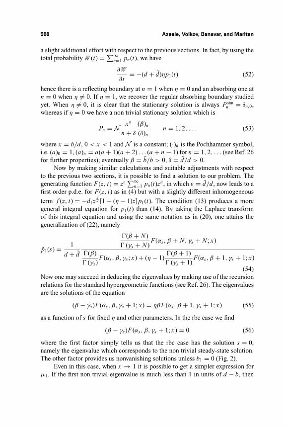
as a function of s for fixed η and other parameters. In the rbc case we find

(β − γs)F(αs, β, γs + 1; x) = 0 (56)

where the first factor simply tells us that the rbc case has the solution s = 0,namely the eigenvalue which corresponds to the non trivial steady-state solution.The other factor provides us nonvanishing solutions unless b1 = 0 (Fig. 2).

Even in this case, when x → 1 it is possible to get a simpler expression forµ1. If the first non trivial eigenvalue is much less than 1 in units of d − b, then


|s/(d − b)| 1 and now we can write

µ1 = (d − b)

∣∣∣∣F(α0, β, γ0 + 1; 1)

∂ς=0 F(αs, β, γs + 1; 1)

∣∣∣∣ (57)

where ς = s/(d − b). As before we can exploit the value of F(a, b, c; 1) to obtainat leading order

µ1 = (d − b)1

|�(β + 1) + γ | (58)

where �(z) is the logarithmic derivative of the gamma function (see Ref. 22) andγ = 0.577 . . . is the Euler’s constant. As µ1 1 one also needs that 1 β < b/b.

When the time is about µ−11 , the solution in (26) is dominated by the first

eigenfunction. In general this latter is different in the reflecting and absorbingboundaries and the eigenvalues are distinct as well. Anyway, if µ

(ref)1 (µ(abs)

1 ) isthe first eigenvalue for the reflecting (absorbing) case, it is possible to see thatµ

(ref)1 < µ

(abs)1 for β � 1 (by using the Eqs. (49) and (58)). Therefore within

this regime, the absorbing stationary solution is reached more rapidly than thereflecting one.

In order to derive the eigenfunctions φ�n , we can proceed as above. Even in

this case the previous remarks about the uniform convergence of∫ ∞

0 F(z, t)e−st d thold. The solution of the Laplace transformed equation now has the form

F(z, s) = C(z, s) + [D(z, s) + (η − 1)E(z, s)] p1(s) (59)

where C(z, s) and D(z, s) are as above and

E(z, s) = βzβ+1(1 − z)β−γs (1 − xz)αs−1

×∫ 1

0dt tβ(1 − zt)γs−β−1(1 − xzt)−αs (60)

Now we may obtain the eigenfunctions by expanding D(z, s) + (η − 1)E(z, s) inpowers of z. Such an expansion produces for n, � = 1, 2, . . .

φ�n = N

n−1∑

k=0

[1

k + β+ (η − 1)

1 − δn,1

k + β + 1

]

×P (� , σ�−1−k)k (2x − 1)P (−� , n−1−k−σ�)

n−1−k (2x − 1) (61)

where N is a constant and the other quantities are defined as in (39).If we use left eigenvectors, then we gain for the solution of the Laplace

transformed equation

G(z, s) = C(z, s) + [D(z, s) + (η − 1)E(z, s)]q1(s) (62)


where the new function is

E(z, s) = d + d

bzβ+1(1 − z)β−γs (1 − z

x)αs−1

×∫ 1

0d t t β(1 − zt)γs−β−1(1 − z

xt)−αs (63)

and the coefficients are defined as in (43).

5. CONCLUSIONS

In this paper we have obtained a spectral resolution of a linear birth-deathprocess by exploiting the properties of the solution of the Laplace transformedequation of the process. Our self-contained approach allowed us to obtain theeigenvectors and the relative eigenvalues of a more general problem (which in-cludes both absorbing and reflecting boundaries).

One of the main applications of this spectral resolution concerns populationdynamics. When studying ecosystems, it is possible to take into account an asym-metry between rare and common species by introducing linear birth and deathrates, i.e. bn = bn + b and dn = dn + d respectively (for an arbitrary specieswith n individuals). If there is no immigration or speciation, one should solve themaster equation with an artificial absorbing boundary at n = 0. It is important tostress that, even though the stationary solution is trivial, the first eigenfunctionof pn(t) can still be interpreted as the population distribution of a given specieson time scales µ−1

1 , where µ1 is the first eigenvalue. Two major simplificationsof our analysis are the non-interacting ideal gas like assumption and ignoring theeffects of the spatial distribution. It would be interesting to probe what qualitativechanges arise on going beyond the mean field-like theory presented here.

APPENDIX A: EIGENFUNCTIONS

In this Appendix we wish to expand the function D(z, s) defined in (35) toobtain the eigenfunctions of pn(t). By using the identity obtained in (B2), we mayat once write the integral inside D(z, s) (because of the uniform convergence ofthe series) in the following form

∫ 1

0d t tβ−1(1 − zt)αs−σ (1 − xzt)−αs

=∞∑

i=0

(σ )i

i!F(−i, αs, σ ; 1 − x)zi

∫ 1

0t i+β−1dt

=∞∑

i=0

(σ )i

i + βF(−i, αs, σ ; 1 − x)

zi

i!


Fig. 2. The upper figure shows the first two nontrivial roots of F(αs , β, γs + 1; x) as a function of swhen b = 1, d = 2, b = 4, d = 3 in the rbc case. For the same parameters the lower figure shows thefirst five nontrivial roots.

where we have defined σ ≡ 2 + d/d − b/b; β > 0, αs as in (20). The other prod-uct is

(1 − z)β−γs (1 − xz)αs−1

=∞∑

m=0

(τ )m

m!F(−m, 1 − αs, τ ; 1 − x)zm

with τ ≡ b/b − d/d. As φ�(z) ∝ D(z,−µ�), then φ�(z) is proportional to

zd/d∞∑

n=1

zn∞∑

m,i=0

(τ )m

m!

(σ )i

i!(i + β)F(−i, α�, σ ; 1 − x)

×F(−m, 1 − α�, τ ; 1 − x)δm+i+1,n

= zd/d∞∑

n=1

znn−1∑

i=0

(σ )i

i!(i + β)F(−i, α�, σ ; 1 − x)


× (τ )n−1−i

(n − 1 − i)!F(i + 1 − n, 1 − α�, τ ; 1 − x)

where α� is αs in which we have set s = −µ�. Thus, owing to the definitions in(28) the following relation holds when n, � = 1, 2, . . .

φ�n ∝

n−1∑

i=0

(σ )i

i!(i + β)F(−i, α�, σ ; 1 − x)

× (τ )n−1−i

(n − 1 − i)!F(i + 1 − n, 1 − α�, τ ; 1 − x)

(A1)

Now we may simplify this formula by making use of the definition of the Jacobi’spolynomials in (B3) of the Appendix B. Finally one achieves

φ�n ∝

n−1∑

i=0

1

i + βP (1−τ , α�−i+τ−2)

i (2x − 1)

× P (τ−1 , n−i−τ−α�)n−1−i (2x − 1)

which is our desired result.

APPENDIX B: GENERATING FUNCTION

OF THE HYPERGEOMETRIC POLYNOMIALS

It is well-known that one can achieve an integral representation (see Ref. 22)of the hypergeometric series that is defined not only for |z| < 1, but is analytic inthe whole complex plane excluding the z-plane cut along the real segment [1,∞].It can be written as

F(α, β, γ ; z) = �(γ )

�(β)�(γ − β)

×∫ 1

0tβ−1(1 − t)γ−β−1(1 − zt)−αd t (B1)

if we assume that �(γ ) > �(β) > 0 and |arg(1 − z)| < π . If either α or β is zeroor a negative integer, the hypergeometric series is a polynomial in z and then therepresentation (B1) is no longer a multivalued function. When α = −n or β = −nthe series is a polynomial of degree n: these are the hypergeometric polynomials.In this case, if we multiply such a polynomial by (γ )n

n! yn and sum over n, we get

∞∑

n=0

(γ )n

n!F(−n, β, γ ; z)yn = �(γ )

�(β)�(γ − β)


×∞∑

n=0

(γ )n

n!

∫ 1

0tβ−1(1 − t)γ−β−1((1 − zt)y)ndt

with y ∈ R under the temporary assumption that the series converges. Due tothe uniform convergence of the argument, it is justified to reverse the order ofsummation and integration. Noting that

∞∑

n=0

(γ )n

n!((1 − zt)y)n = F(γ, 1, 1; (1 − zt)y) = (1 − y + t zy)−γ

we can write

∞∑

n=0

(γ )n

n!F(−n, β, γ ; z)yn = �(γ )

�(β)�(γ − β)

×∫ 1

0tβ−1(1 − t)γ−β−1(1 − y + t zy)−γ d t

Under the transformation ζ = zyy−1 , the r.h.s. of the previous equation is equal to

(1 − y)−γ �(γ )

�(β)�(γ − β)

∫ 1

0tβ−1(1 − t)γ−β−1(1 − ζ t)−γ d t

= (1 − y)−γ F(γ, β, γ ;zy

y − 1)

Hence for |y| < min{1, 1|z−1| }

∞∑

n=0

(γ )n

n!F(−n, β, γ ; z)yn = (1 − y)β−γ (1 − y + zy)−β (B2)

when γ �= 0,−1,−2, . . .. Thus we have achieved the generating function of thehypergeometric polynomials. It is interesting to note that these polynomials are notorthogonal with respect to the z variable. If we write the hypergeometric equationin the self-adjoint form, one can readily prove that the orthogonal polynomials inthe real interval [0, 1] with respect to the weight function zγ−1(1 − z)δ−γ−1 areF(−n, n + δ − 1, γ ; z) (provided that z, δ, γ are real and δ > γ > 0). If we setγ = α + 1 and δ = α + β + 2, it is possible to identify these polynomials withthose of Jacobi (see Ref. 21):

F(−n, n + α + β + 1, α + 1; z) = n!

(α + 1)nP (α,β)

n (1 − 2z) (B3)


Nevertheless if we set β = −i (i ∈ N) in (B2) and we multiply such an equationby (γ )i

i! ( 11−z )i F(−m,−i, γ ; z) and sum over i , we get

∞∑

i,n=0

(γ )i

i!

F(−m,−i, γ ; z)

(1 − z)i

(γ )n

n!

F(−n,−i, γ ; z)

(1 − z)n=

[z − 1

z

]γ

after putting y = 1/(1 − z). This leads to the orthogonality relation

∞∑

i=0

(γ )i

i!

1

(1 − z)iF(−m,−i, γ ; z)F(−n,−i, γ ; z)

= δm,n(1 − z)nn!

(γ )n

(z − 1

z

)γ

(B4)

We may define Mn(i ; γ, x) ≡ (γ )n F(−n,−i, γ ; 1 − 1x ) and finally we achieve

(here x−1 = 1 − z)

∞∑

i=0

Mm(i ; γ, x)Mn(i ; γ, x)(γ )i

i!xi = δm,n

n! (1 − x)−γ

(γ )n xn(B5)

when we fix 0 < x < 1 and γ > 0, Mn(i ; γ, x) are the Meixner polynomials,which are orthogonal with respect to the discrete measure (γ )i

i! xi .

REFERENCES

1. N. G. van Kampen, Stochastic Processes in Physics and Chemistry, Elsevier (2004).2. W. Feller, An Introduction to Probability Theory and its Applications, Vol. I, Wiley, NJ (1968).3. C. A. Condat, Defect diffusion and closed-time distributions for ionic channels in cell membranes.

Phys. Rev. A 39:2112–2125 (1989).4. N. G. van Kampen and I. Oppenheim, Expansion of the master equation for one-dimensional

random walks with boundary. J. Math. Phys. 13:842–849 (1972).5. D. R. Cox and W. L. Smith, Queues, Methuen, New York (1961).6. S. Karlin and J. McGregor, Linear growth, birth and death processes. J. Math. Mech. 7:643–661

(1958).7. S. Karlin and J. McGregor, The classification of birth and death processes. Trans. Amer. Math.

Soc. 86:366–401 (1957).8. S. Karlin and J. McGregor, The differential equations of birth and death processes and the stieltjes

moment problem. Trans. Amer. Math. Soc. 86:489–546 (1957).9. M. E. H. Ismail, J. Letessier and G. Valent, Linear birth and death models and associated laguerre

and meixner polynomials. J. of Approx. Th. 55:337–348 (1988).10. S. P. Hubbell, The Unified Neutral Theory of Biodiversity and Biogeography, Princeton University

Press, NJ (2001).11. I. Volkov, J. R. Banavar, S. P. Hubbell and A. Maritan, Neutral theory and relative species abundance

in ecology. Nature 424:1035–1037 (2003).12. I. Volkov, J. R. Banavar, F. He, S. P. Hubbell and A. Maritan, Density dependence explains tree

species abundance and diversity in tropical forests. Nature 438:658–661 (2005).


13. S. Pigolotti, A. Flammini and A. Maritan, Stochastic model for the species abundance problem inan ecological community. Phys. Rev. E 70:011916 (2004).

14. S. Karlin and H. Taylor, A First Course in Stochastic Processes, Academic Press (1975).15. W. Feller, Two singular diffusion problems. Ann. of Math. 54:173–182 (1951).16. W. Ledermann and G. E. H. Reuter, Spectral theory for the differential equations of simple birth

and death processes. Phil. Trans. Royal Soc. Lon. A 246:321–369 (1954).17. R. C. F. Bartels and R. V. Churchill, Resolution of boundary problems by the use of a generalized

convolution. Bull. Am. Math. Soc. 48:276–282 (1942).18. R. Courant and D. Hilbert, Methods of Mathematical Physics, Wiley (1989).19. I. N. Sneddon, Elements of Partial Differential Equations, McGraw-Hill (1957).20. F. G. Tricomi, Integral Equations, Dover (1985).21. M. Abramowitz and I. A. Stegun, Handbook of mathematical functions. Nat. Bur. of Stand. (1964).22. N. N. Lebedev, Special Functions and their Applications, Dover (1972).23. T. S. Chihara, An Introduction to Orthogonal Polynomials, Gordon & Breach, New York (1978).24. A. Erdelyi, W. Magnus, F. Oberhettinger and F.G. Tricomi, Higher Trascendental Functions, Vol.

II, McGraw-Hill, New York (1953).25. E. T. Whittaker and G. N. Watson, A Course of Modern Analysis, Cambridge University Press

(1963).26. I. S. Gradshteyn and I. M. Ryzhik, Table of Integrals, Series and Products, Academic Press (2000).

linear one-step processes with artiﬁcial boundariesfbssaz/articles/azaele_jsp06.pdf ·...

Documents