Linear Programming Problem

Introduction

• Linear Programming was developed by

George B Dantzing in 1947 for solving

military logistic operations.

• Meaning of Linear Programming

– The word Linear refers to linear relationship

among variables. i.e. a given change in one

variable will always cause a resulting

proportional change in another variable. For

example, doubling the investment on a

certain project will exactly double the rate of

return.

Introduction

• The word programming refers to modeling

& solving a problem mathematically that

involves the economic allocation of limited

resources by choosing a strategy among

various alternative strategies to achieve the

desired objective.

Introduction

• Linear Programming (LP) is a mathematical

modeling technique useful for the allocation of

limited resources, such as labour, material,

machine, time, warehouse space, capital,

energy etc. to several competing activities,

such as products, services, jobs, new projects

etc.

Introduction

Introduction

• Also, the general LPP calls for optimizing a

linear function of variables called the

objective function subject to a set of linear

equations and /or inequalities called the

constraints or restrictions.

General Structure of LPP

• Decision Variables

• The Objective Function

• The Constraints

General Structure of LPP

• Decision Variables: The activities that are

competing one another for sharing the

resources available. These variables are

usually interrelated in terms of utilization of

resources and need simultaneous solutions.

All these variables are considered as

continuous, controllable and non-negative.

General Structure of LPP

• The Objective Function: A LPP must have

an objective which should be clearly

identifiable and measurable in quantitative

terms. It could be of maximization of profit

(sales), minimization of cost etc. The

relationship among variables representing

objective must be linear.

General Structure of LPP

• The Constraints: There are always certain

limitations or restrictions or constraints on the use of

resources, such as labour, space, raw material,

money etc. that limit the degree to which an objective

can be achieved. Such constraints must be

expressed as linear inequalities or equations in terms

of decision variables.

Assumptions of LP Model

• Certainty

• Additivity

• Linearity (Proportionality)

• Divisibility (continuity)

Assumptions of LP Model

• Certainty: In all LLP’s, it is assumed that all the

parameters; such as availability of resources,

profit contribution of a unit or cost contribution

of a unit of decision variable and computation of

resources by a unit decision variable must be

known and fixed. Or we can say that, all the

coefficients in this objective function as well as

in the constraints are completely known with

certainty and do not change during the period

Assumptions of LP Model

of study. Thus, the profit per unit of the

product, requirements of material and labour

per unit, availability of material etc. are given

and known in the problem. The LP is

obviously deterministic in nature.

Assumptions of LP Model

• Additivity: The value of the obj. function for the

given values of decision variables and the total

sum of resources used, must be equal to the

sum of the contributions (profit or loss) earned

from each decision variable and the sum of the

resources used by each decision variable

respectively. For example, the total profit

earned by the sale of two products A & B must

Assumptions of LP Model

be equal to the sum of the profits earned

separately from A & B. Similarly, the amount

of a resource consumed by A & B must be

equal to the sum of resources used for A & B

individually.

Assumptions of LP Model

• Linearity or Proportionality: This assumption

requires the contribution of each decision

variable in both the obj function and the

constraints to be directly proportional to the

value of the decision variable. Or we can say

that, the amount of each resource used ( or

supplied) and its contribution to the profit (or

cost) in obj. fun must be proportional to the

value of each decision variable. For eg., if

Assumptions of LP Model

production of a one unit of a product uses 5

hrs of a particular resource, then making 3

units of that product uses 3*5=15 hrs of that

resource.

Assumptions of LP Model

• Divisibility or Continuity: This implies that

solution values of the decision variables and

resources can take on any non-negative values,

including fractional values of the decision

variables. For eg., it is possible to produce 8.35

quintals of wheat or 7.453 thousand gallons of a

solvent or 43.45 thousand kiloliters of milk. Such

variables are not divisible and hence are to be

assigned

Assumptions of LP Model

integer values. When it is necessary to have

integer variables, the integer programming

problem is considered to attain the desired

values.

Formulation of LPP

The term formulation referred to the process

of converting the verbal description and

numerical data into mathematical expressions

which represents the relationship among

relevant decision variable (factors), objective

& restrictions on the use of resources.

Introduction

• The term formulation referred to the process

of converting the verbal description and

numerical data into mathematical expressions

which represents the relationship among

relevant decision variable (factors), objective

& restrictions on the use of resources.

Introduction

The XYZ garment company manufactures

men's shirts and women’s t-shirts for ABC

Discount stores. ABC will accept all the

production supplied by the company. The

production process includes cutting, sewing

and packaging. XYZ employs 25 workers in the

cutting department, 35 in the sewing

department and 5 in the packaging department.

The factory works one 8-hour shift, 5 days a

week.

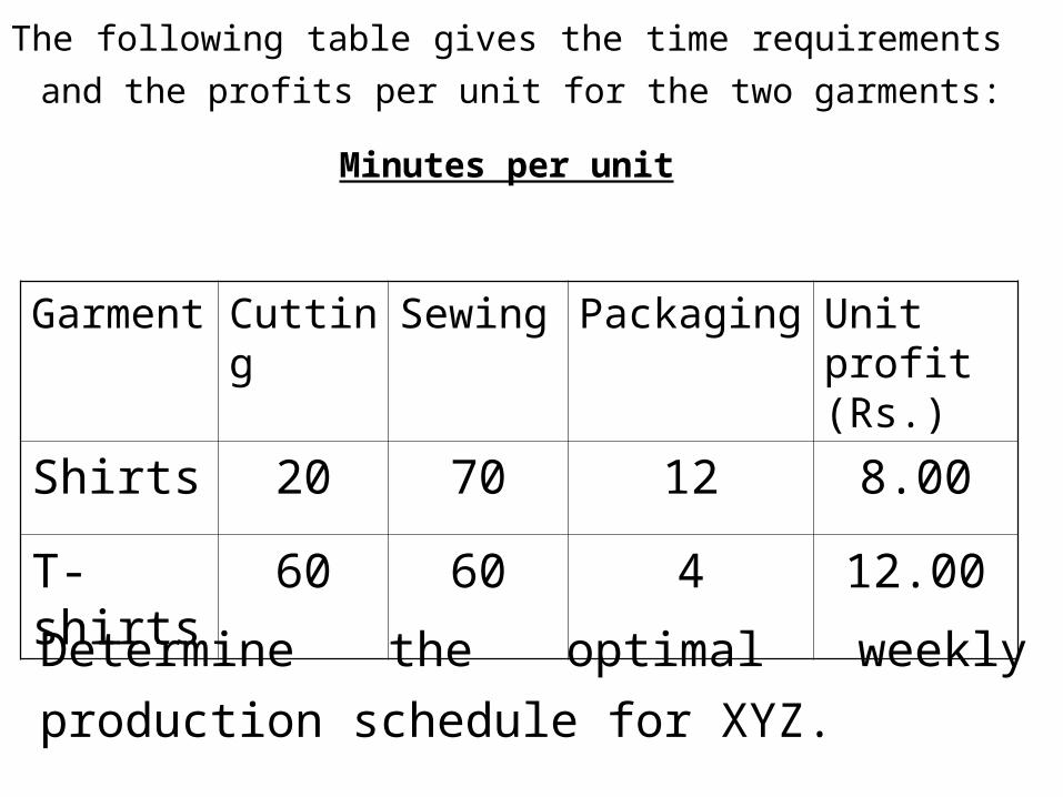
The following table gives the time requirements

and the profits per unit for the two garments:

Minutes per unit

Garment Cutting Sewing Packaging Unit profit (Rs.)

Shirts 20 70 12 8.00

T-shirts 60 60 4 12.00

Determine the optimal weekly production

schedule for XYZ.

Solution

Assume that XYZ produces x1 shirts and x2 t-

shirts per week.

8 x1 + 12 x2Profit got =

Time spent on cutting = 20 x1 + 60 x2 mts

Time spent on sewing = 70 x1 + 60 x2 mts

Time spent on packaging = 12 x1 + 4 x2 mts

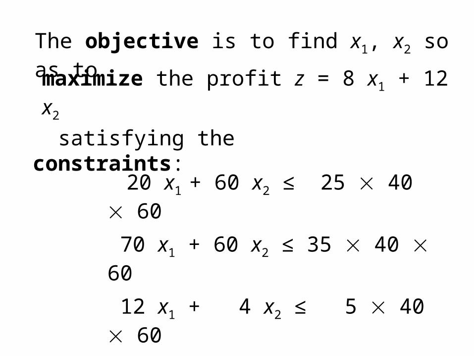
maximize the profit z = 8 x1 + 12 x2

The objective is to find x1, x2 so as to

satisfying the constraints:

20 x1 + 60 x2 ≤ 25 40 60

70 x1 + 60 x2 ≤ 35 40 60

12 x1 + 4 x2 ≤ 5 40 60

x1, x2 ≥ 0, integers

This is a typical optimization problem.

Any values of x1, x2 that satisfy all the

constraints of the model is called a feasible

solution. We are interested in finding the

optimum feasible solution that gives the

maximum profit while satisfying all the

constraints.

More generally, an optimization problem looks

as follows:

Determine the decision variables x1, x2, …,

xn so as to optimize an objective function f

(x1, x2, …, xn) satisfying the constraints

gi (x1, x2, …, xn) ≤ bi (i=1, 2, …, m).

Linear Programming Problems(LPP)

An optimization problem is called a Linear

Programming Problem (LPP) when the

objective function and all the constraints are

linear functions of the decision variables, x1,

x2, …, xn. We also include the “non-negativity

restrictions”, namely xj ≥ 0 for all j=1, 2, …, n.

Thus a typical LPP is of the form:

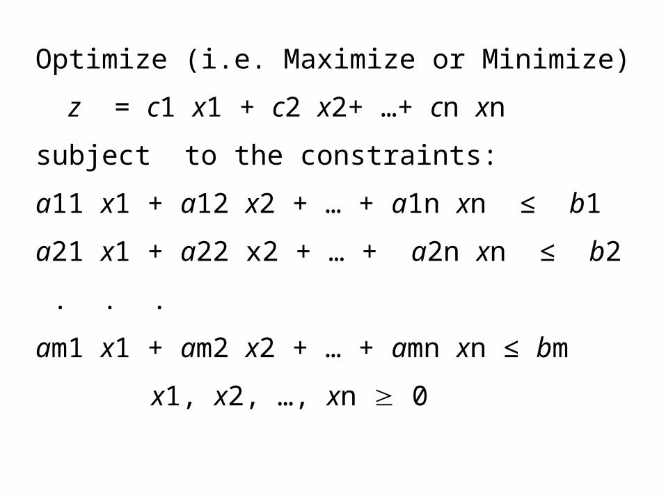
Optimize (i.e. Maximize or Minimize)

z = c1 x1 + c2 x2+ …+ cn xn

subject to the constraints:

a11 x1 + a12 x2 + … + a1n xn ≤ b1

a21 x1 + a22 x2 + … + a2n xn ≤ b2

. . .

am1 x1 + am2 x2 + … + amn xn ≤ bm

x1, x2, …, xn 0

Advantages and Limitations

Application Areas of Linear Programming

Advantages• LP helps in attaining the optimum use of

productive resources. It also indicates how a

decision maker can employ his productive

factors effectively by selecting and distributing

these resources.

• LP technique improves the quality of decisions.

• LP technique provides possible and pratical

solutions since there might be other constraints

operating operating outside the problem which

must be taken into account.

Advantages

• LP also helps in re-valuation of a basic plan for

changing conditions. If conditions change when

the plan is partly carried out, they can be

determined so as to adjust the remainder of the

plan for best results.

Limitations

• LP treats all relationship s among variables as

linear.

• While solving the an LPP, there is no guarntee

that we will get integer valued solutions.

• LP model does not take into consideration the

effect of time and uncertainnity.

Limitations

• Parameters appearing in the model are

assumed to be constant but in real-life

situations, they are frequently neither klnown

nor constant.

• It deals with single objective, whereas in real-

life situations we may come across conflicting

multi-objective problems.

Applications

• Agriculture Applications

• Military Operations

• Production Management

• Financial Management

• Marketing Managemant

• Personnel Management

General Structure of LPP

The general LPP with n decision variables and

m constraints can be stated as:

Find the values of decision variables…..

Steps for formulating the LPP

• Identify the Decision Variabels

• Identify the Problem data

• Formulate the constraints

• Formulate the Objective Function