linear regression and correlation explanatory and response variables are numeric relationship...
TRANSCRIPT

Linear Regression and Correlation
• Explanatory and Response Variables are Numeric• Relationship between the mean of the response
variable and the level of the explanatory variable assumed to be approximately linear (straight line)
• Model:
),0(~10 NxY
• 1 > 0 Positive Association
• 1 < 0 Negative Association
• 1 = 0 No Association

Least Squares Estimation of 0, 1
0 Mean response when x=0 (y-intercept)
1 Change in mean response when x increases by 1 unit (slope)
• 0, 1 are unknown parameters (like )
• 0+1x Mean response when explanatory variable takes on the value x
• Goal: Choose values (estimates) that minimize the sum of squared errors (SSE) of observed values to the straight-line:
2
1 1
^
0
^
1
2^
10
^
n
i ii
n
i ii xyyySSExbby

Example - Pharmacodynamics of LSD
Score (y) LSD Conc (x)78.93 1.1758.20 2.9767.47 3.2637.47 4.6945.65 5.8332.92 6.0029.97 6.41
• Response (y) - Math score (mean among 5 volunteers)
• Predictor (x) - LSD tissue concentration (mean of 5 volunteers)
• Raw Data and scatterplot of Score vs LSD concentration:
LSD_CONC
7654321
SC
OR
E
80
70
60
50
40
30
20
Source: Wagner, et al (1968)
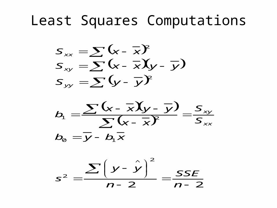
Least Squares Computations
22
2^
2
10
21
2
2
n
SSE
n
yys
xbyb
S
S
xx
yyxxb
yyS
yyxxS
xxS
xx
xy
yy
xy
xx

Example - Pharmacodynamics of LSD
72.5001.910.89
10.89)33.4)(01.9(09.5001.94749.22
4872.202
333.47
33.30087.50
7
61.350
2^
1
^
01
sxy
xybb
xy
Score (y) LSD Conc (x) x-xbar y-ybar Sxx Sxy Syy78.93 1.17 -3.163 28.843 10.004569 -91.230409 831.91864958.20 2.97 -1.363 8.113 1.857769 -11.058019 65.82076967.47 3.26 -1.073 17.383 1.151329 -18.651959 302.16868937.47 4.69 0.357 -12.617 0.127449 -4.504269 159.18868945.65 5.83 1.497 -4.437 2.241009 -6.642189 19.68696932.92 6.00 1.667 -17.167 2.778889 -28.617389 294.70588929.97 6.41 2.077 -20.117 4.313929 -41.783009 404.693689350.61 30.33 -0.001 0.001 22.474943 -202.487243 2078.183343
(Column totals given in bottom row of table)

SPSS Output and Plot of EquationCoefficientsa
89.124 7.048 12.646 .000
-9.009 1.503 -.937 -5.994 .002
(Constant)
LSD_CONC
Model1
B Std. Error
UnstandardizedCoefficients
Beta
StandardizedCoefficients
t Sig.
Dependent Variable: SCOREa.
Linear Regression
1.00 2.00 3.00 4.00 5.00 6.00
lsd_conc
30.00
40.00
50.00
60.00
70.00
80.00
sco
re
score = 89.12 + -9.01 * lsd_concR-Square = 0.88
Math Score vs LSD Concentration (SPSS)
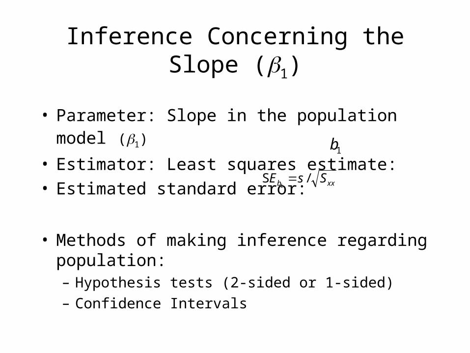
Inference Concerning the Slope (1)
• Parameter: Slope in the population model (1)
• Estimator: Least squares estimate:• Estimated standard error:
• Methods of making inference regarding population:– Hypothesis tests (2-sided or 1-sided)
– Confidence Intervals
1b
xxb SsE /S1

Hypothesis Test for 1
• 2-Sided Test– H0: 1 = 0
– HA: 1 0
• 1-sided Test– H0: 1 = 0
– HA+: 1 > 0 or
– HA-: 1 < 0
|)|(2:value
||:..
:..
2,2/
1
1
obs
nobs
bobs
ttPP
ttRR
SE
btST
)(:)(:
:..:..
:..
2,2,
1
1
obsobs
nobsnobs
bobs
ttPvalPttPvalP
ttRRttRR
SE
btST

(1-)100% Confidence Interval for 1
xx
bS
stbSEtb 2/12/1 1
• Conclude positive association if entire interval above 0
• Conclude negative association if entire interval below 0
• Cannot conclude an association if interval contains 0
• Conclusion based on interval is same as 2-sided hypothesis test
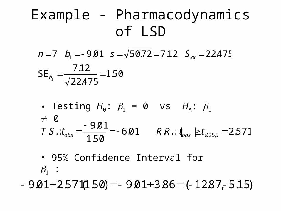
Example - Pharmacodynamics of LSD
50.1475.22
12.7SE
475.2212.772.5001.97
1
1
b
xxSsbn
• Testing H0: 1 = 0 vs HA: 1 0
571.2|:|..01.650.1
01.9:.. 5,025.
ttRRtST obsobs
• 95% Confidence Interval for 1 :
)15.5,87.12(86.301.9)50.1(571.201.9
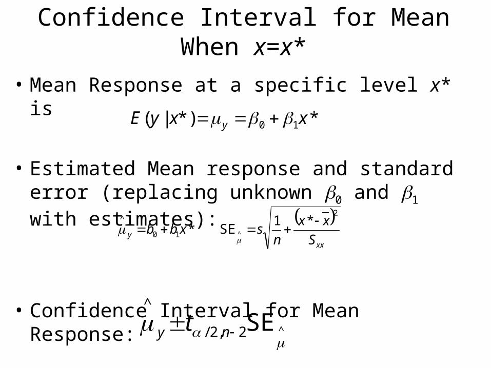
Confidence Interval for Mean When x=x*
• Mean Response at a specific level x* is
• Estimated Mean response and standard error (replacing unknown 0 and 1 with estimates):
• Confidence Interval for Mean Response:
**)|( 10 xxyE y
xx
y S
xx
nsxbb
2
10
^ *1SE* ^
^SE2,2/
^
ny t
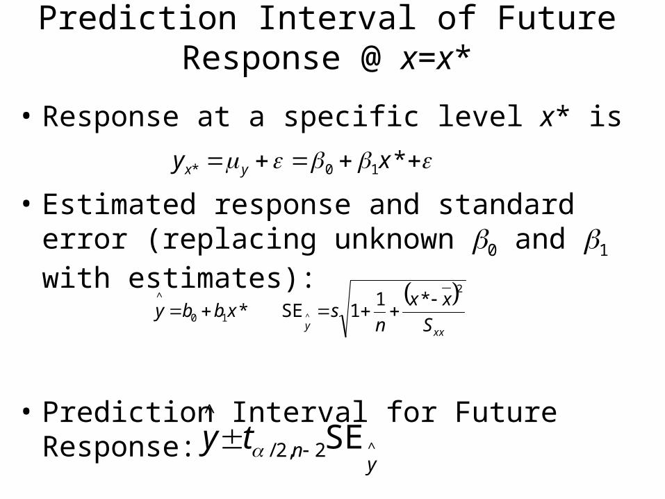
Prediction Interval of Future Response @ x=x*
• Response at a specific level x* is
• Estimated response and standard error (replacing unknown 0 and 1 with estimates):
• Prediction Interval for Future Response:
*10* xy yx
xx
y S
xx
nsxbby
2
10
^ *11SE* ^
^SE2,2/
^
ynty

Correlation Coefficient• Measures the strength of the linear association
between two variables• Takes on the same sign as the slope estimate from
the linear regression• Not effected by linear transformations of y or x• Does not distinguish between dependent and
independent variable (e.g. height and weight)• Population Parameter - • Pearson’s Correlation Coefficient:
11 rSS
Sr
yyxx
xy
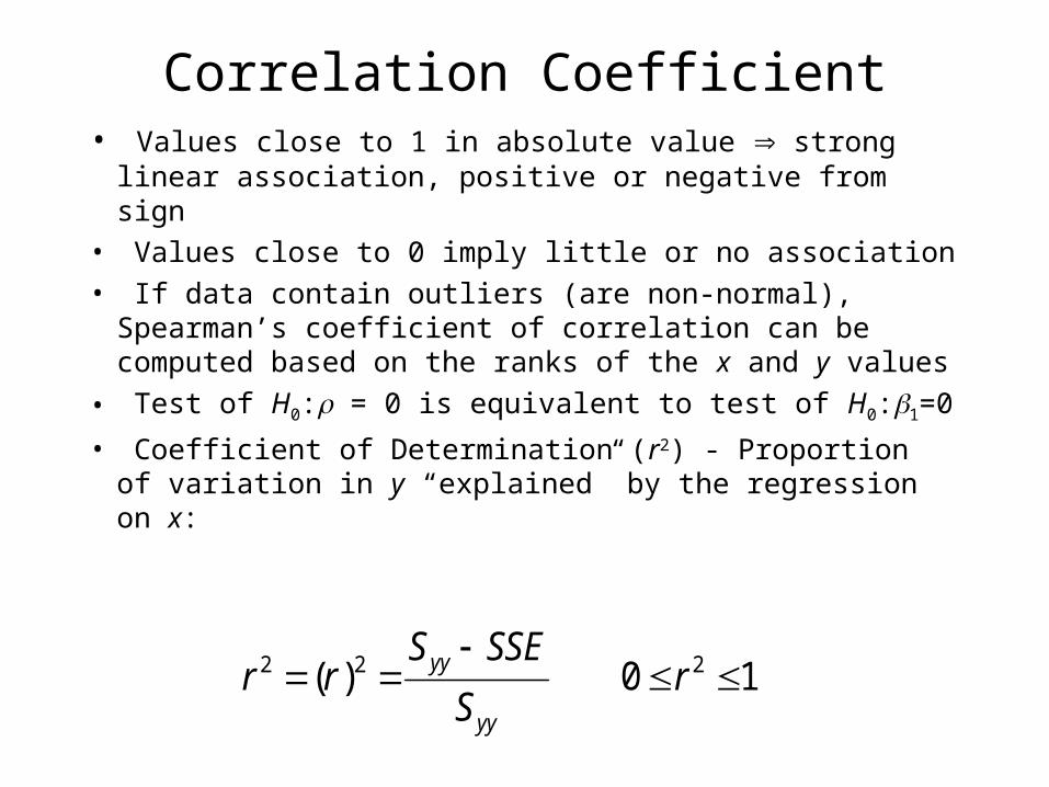
Correlation Coefficient• Values close to 1 in absolute value strong
linear association, positive or negative from sign• Values close to 0 imply little or no association• If data contain outliers (are non-normal),
Spearman’s coefficient of correlation can be computed based on the ranks of the x and y values
• Test of H0: = 0 is equivalent to test of H0:1=0
• Coefficient of Determination (r2) - Proportion of variation in y “explained” by the regression on x:
10)( 222
rS
SSESrr
yy
yy
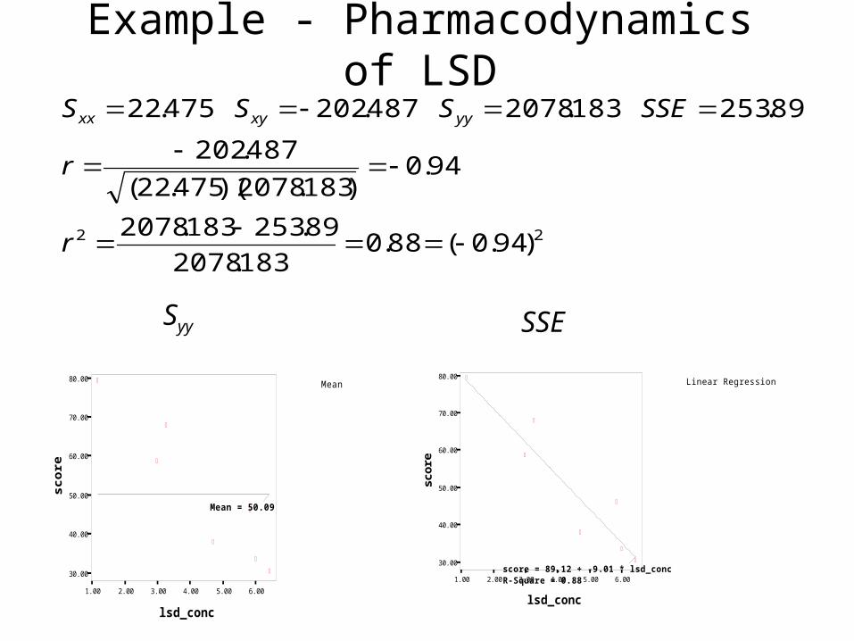
Example - Pharmacodynamics of LSD
22 )94.0(88.0183.2078
89.253183.2078
94.0)183.2078)(475.22(
487.202
89.253183.2078487.202475.22
r
r
SSESSS yyxyxx
Mean
1.00 2.00 3.00 4.00 5.00 6.00
lsd_conc
30.00
40.00
50.00
60.00
70.00
80.00
Mean = 50.09
Linear Regression
1.00 2.00 3.00 4.00 5.00 6.00
lsd_conc
30.00
40.00
50.00
60.00
70.00
80.00
score
score = 89.12 + -9.01 * lsd_concR-Square = 0.88
Syy SSE
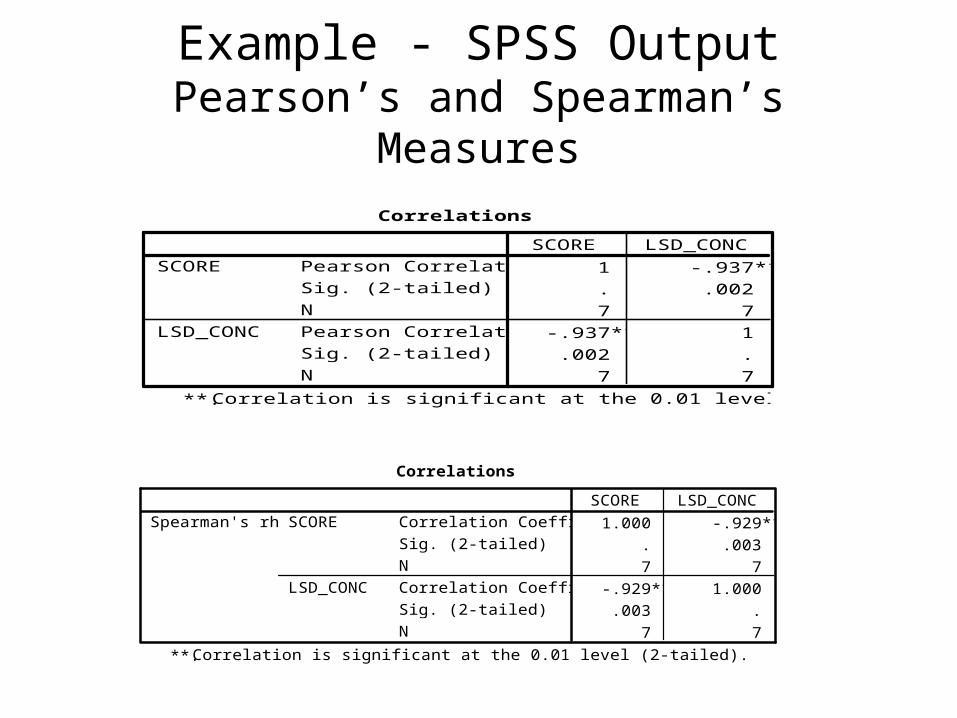
Example - SPSS OutputPearson’s and Spearman’s Measures
Correlations
1 -.937**
. .002
7 7
-.937** 1
.002 .
7 7
Pearson Correlation
Sig. (2-tailed)
N
Pearson Correlation
Sig. (2-tailed)
N
SCORE
LSD_CONC
SCORE LSD_CONC
Correlation is significant at the 0.01 level (2-tailed).**.
Correlations
1.000 -.929**
. .003
7 7
-.929** 1.000
.003 .
7 7
Correlation Coefficient
Sig. (2-tailed)
N
Correlation Coefficient
Sig. (2-tailed)
N
SCORE
LSD_CONC
Spearman's rhoSCORE LSD_CONC
Correlation is significant at the 0.01 level (2-tailed).**.

Analysis of Variance in Regression
• Goal: Partition the total variation in y into variation “explained” by x and random variation
2^2^2
^^
)()()(
)()()(
yyyyyy
yyyyyy
iiii
iiii
• These three sums of squares and degrees of freedom are:
•Total (SST) DFT = n-1
• Error (SSE) DFE = n-2
• Model (SSM) DFM = 1
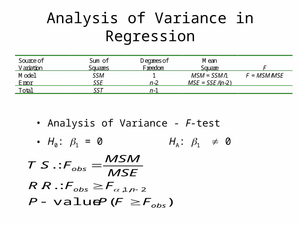
Analysis of Variance in Regression
Source ofVariation
Sum ofSquares
Degrees ofFreedom
MeanSquare F
Model SSM 1 MSM = SSM/1 F = MSM/MSEError SSE n-2 MSE = SSE/(n-2)Total SST n-1
• Analysis of Variance - F-test
• H0: 1 = 0 HA: 1 0
)(:value
:..
:..
2,1,
obs
nobs
obs
FFPP
FFRRMSE
MSMFST

Example - Pharmacodynamics of LSD
• Total Sum of squares:
617183.2078)( 2 DFTyySST i
• Error Sum of squares:
527890.253)( 2^
DFEyySSEii
• Model Sum of Squares:
1293.1824890.253183.2078)( 2^
DFMyySSMi

Example - Pharmacodynamics of LSDSource ofVariation
Sum ofSquares
Degrees ofFreedom
MeanSquare F
Model 1824.293 1 1824.293 35.93Error 253.890 5 50.778Total 2078.183 6
•Analysis of Variance - F-test
• H0: 1 = 0 HA: 1 0
)93.35(:
61.6:..
93.35:..
5,1,05.
FPvalP
FFRRMSE
MSRFST
obs
obs

Example - SPSS Output
ANOVAb
1824.302 1 1824.302 35.928 .002a
253.881 5 50.776
2078.183 6
Regression
Residual
Total
Model1
Sum ofSquares df Mean Square F Sig.
Predictors: (Constant), LSD_CONCa.
Dependent Variable: SCOREb.

Multiple Regression
• Numeric Response variable (Y)• p Numeric predictor variables• Model:
Y = 0 + 1x1 + + pxp +
• Partial Regression Coefficients: i effect (on the mean response) of increasing the ith predictor variable by 1 unit, holding all other predictors constant

Example - Effect of Birth weight on Body Size in Early Adolescence
• Response: Height at Early adolescence (n =250 cases)
• Predictors (p=6 explanatory variables)
• Adolescent Age (x1, in years -- 11-14)
• Tanner stage (x2, units not given)
• Gender (x3=1 if male, 0 if female)
• Gestational age (x4, in weeks at birth)
• Birth length (x5, units not given)
• Birthweight Group (x6=1,...,6 <1500g (1), 1500-1999g(2), 2000-2499g(3), 2500-2999g(4), 3000-3499g(5), >3500g(6))Source: Falkner, et al (2004)

Least Squares Estimation
• Population Model for mean response:
pp xxYE 110)(
• Least Squares Fitted (predicted) equation, minimizing SSE:
2^
110
^
YYSSExbxbbY pp
• All statistical software packages/spreadsheets can compute least squares estimates and their standard errors
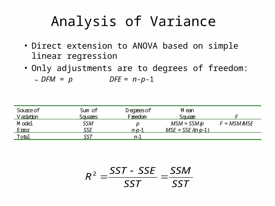
Analysis of Variance
• Direct extension to ANOVA based on simple linear regression
• Only adjustments are to degrees of freedom:– DFM = p DFE = n-p-1
Source ofVariation
Sum ofSquares
Degrees ofFreedom
MeanSquare F
Model SSM p MSM = SSM/p F = MSM/MSEError SSE n-p-1 MSE = SSE/(n-p-1)Total SST n-1
SST
SSM
SST
SSESSTR
2
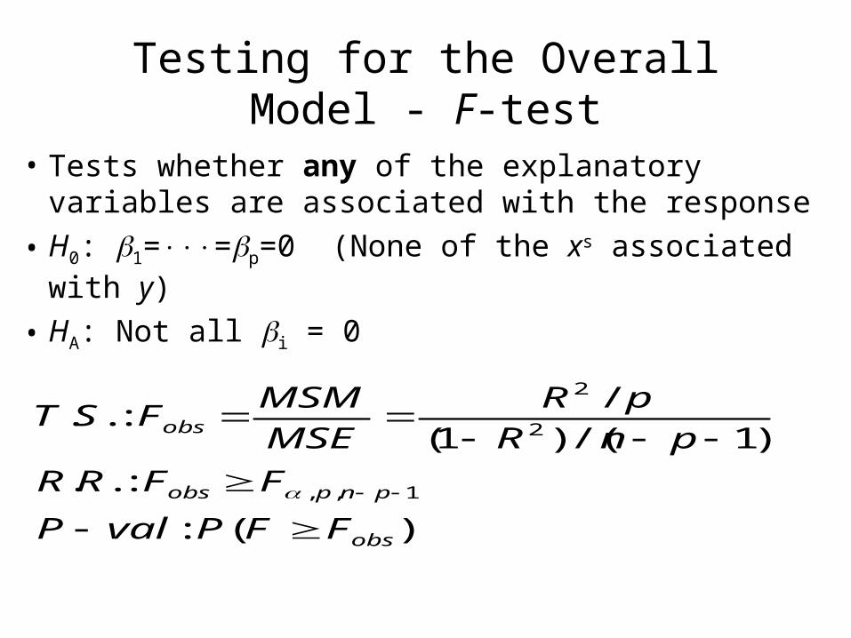
Testing for the Overall Model - F-test
• Tests whether any of the explanatory variables are associated with the response
• H0: 1==p=0 (None of the xs associated with y)
• HA: Not all i = 0
)(:
:..
)1/()1(
/:..
1,,
2
2
obs
pnpobs
obs
FFPvalP
FFRR
pnR
pR
MSE
MSMFST

Example - Effect of Birth weight on Body Size in Early Adolescence
• Authors did not print ANOVA, but did provide following:
• n=250 p=6 R2=0.26• H0: 1==6=0• HA: Not all i = 0
)2.14(:
13.2:..
2.140030.
0433.
)16250/()26.01(
6/26.0
)1/()1(
/:..
243,6,
2
2
FPvalP
FFRR
pnR
pR
MSE
MSRFST
obs
obs

Testing Individual Partial Coefficients - t-tests
• Wish to determine whether the response is associated with a single explanatory variable, after controlling for the others
• H0: i = 0 HA: i 0 (2-sided alternative)
|)|(2:
||:..
SE:..
1,2/
obs
pnobs
b
iobs
ttPvalP
ttRR
btST
i
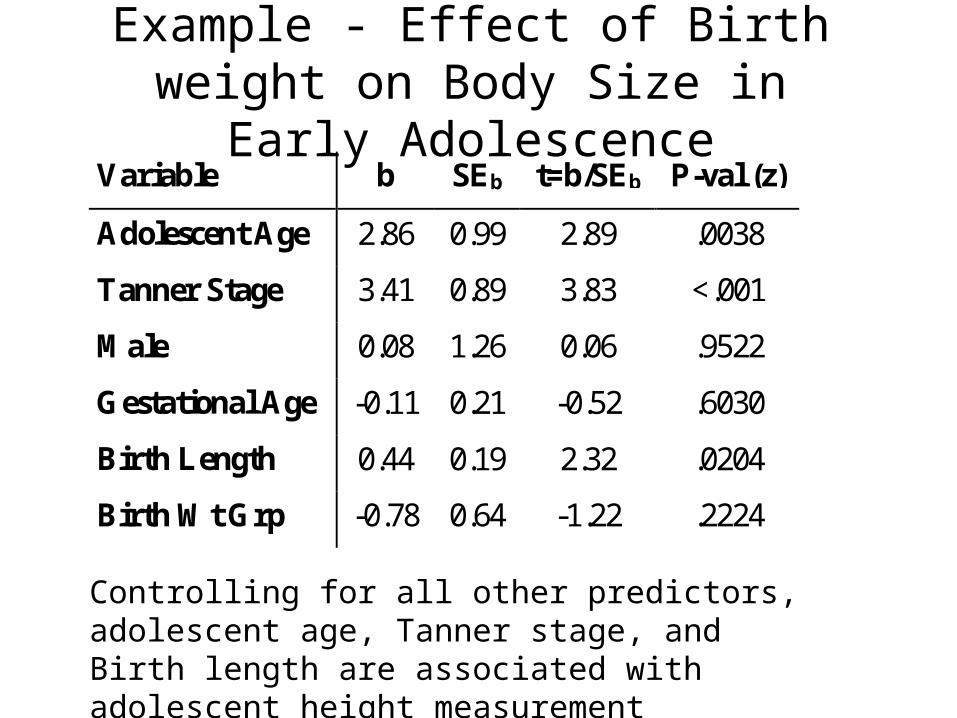
Example - Effect of Birth weight on Body Size in Early Adolescence
Variable b SEb t=b/SEb P-val (z)
Adolescent Age 2.86 0.99 2.89 .0038
Tanner Stage 3.41 0.89 3.83 <.001
Male 0.08 1.26 0.06 .9522
Gestational Age -0.11 0.21 -0.52 .6030
Birth Length 0.44 0.19 2.32 .0204
Birth Wt Grp -0.78 0.64 -1.22 .2224
Controlling for all other predictors, adolescent age, Tanner stage, and Birth length are associated with adolescent height measurement

Testing for the Overall Model - F-test
• Tests whether any of the explanatory variables are associated with the response
• H0: 1==p=0 (None of Xs associated with Y)
• HA: Not all i = 0
)(:
)1/()1(
/:..
2
2
obs
obs
FFPvalP
pnR
pR
MSE
MSRFST
The P-value is based on the F-distribution with p numerator and (n-p-1) denominator degrees of freedom

Comparing Regression Models
• Conflicting Goals: Explaining variation in Y while keeping model as simple as possible (parsimony)
• We can test whether a subset of p-g predictors (including possibly cross-product terms) can be dropped from a model that contains the remaining g predictors. H0: g+1=…=p =0
– Complete Model: Contains all k predictors
– Reduced Model: Eliminates the predictors from H0
– Fit both models, obtaining the Error sum of squares for each (or R2 from each)

Comparing Regression Models
• H0: g+1=…=p = 0 (After removing the effects of X1,…,Xg, none of other predictors are associated with Y)
• Ha: H0 is false
)(
]1/[
)/()( :StatisticTest
obs
c
crobs
FFPP
pnSSE
gpSSESSEF
P-value based on F-distribution with p-g and n-p-1 d.f.
Models with Dummy Variables
• Some models have both numeric and categorical explanatory variables (Recall gender in example)
• If a categorical variable has k levels, need to create k-1 dummy variables that take on the values 1 if the level of interest is present, 0 otherwise.
• The baseline level of the categorical variable for which all k-1 dummy variables are set to 0
• The regression coefficient corresponding to a dummy variable is the difference between the mean for that level and the mean for baseline group, controlling for all numeric predictors

Example - Deep Cervical Infections• Subjects - Patients with deep neck infections
• Response (Y) - Length of Stay in hospital
• Predictors: (One numeric, 11 Dichotomous)– Age (x1)
– Gender (x2=1 if female, 0 if male)
– Fever (x3=1 if Body Temp > 38C, 0 if not)
– Neck swelling (x4=1 if Present, 0 if absent)
– Neck Pain (x5=1 if Present, 0 if absent)
– Trismus (x6=1 if Present, 0 if absent)
– Underlying Disease (x7=1 if Present, 0 if absent)
– Respiration Difficulty (x8=1 if Present, 0 if absent)
– Complication (x9=1 if Present, 0 if absent)
– WBC > 15000/mm3 (x10=1 if Present, 0 if absent)
– CRP > 100g/ml (x11=1 if Present, 0 if absent)
Source: Wang, et al (2003)
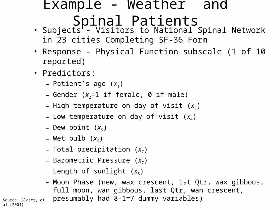
Example - Weather and Spinal Patients• Subjects - Visitors to National Spinal Network in 23 cities
Completing SF-36 Form• Response - Physical Function subscale (1 of 10 reported)• Predictors:
– Patient’s age (x1)
– Gender (x2=1 if female, 0 if male)
– High temperature on day of visit (x3)
– Low temperature on day of visit (x4)
– Dew point (x5)
– Wet bulb (x6)
– Total precipitation (x7)
– Barometric Pressure (x7)
– Length of sunlight (x8)
– Moon Phase (new, wax crescent, 1st Qtr, wax gibbous, full moon, wan gibbous, last Qtr, wan crescent, presumably had 8-1=7 dummy variables)
Source: Glaser, et al (2004)

Analysis of Covariance
• Combination of 1-Way ANOVA and Linear Regression
• Goal: Comparing numeric responses among k groups, adjusting for numeric concomitant variable(s), referred to as Covariate(s)
• Clinical trial applications: Response is Post-Trt score, covariate is Pre-Trt score
• Epidemiological applications: Outcomes compared across exposure conditions, adjusted for other risk factors (age, smoking status, sex,...)

Nonlinear Regression
• Theory often leads to nonlinear relations between variables. Examples:
– 1-compartment PK model with 1st-order absorption and elimination
– Sigmoid-Emax S-shaped PD model

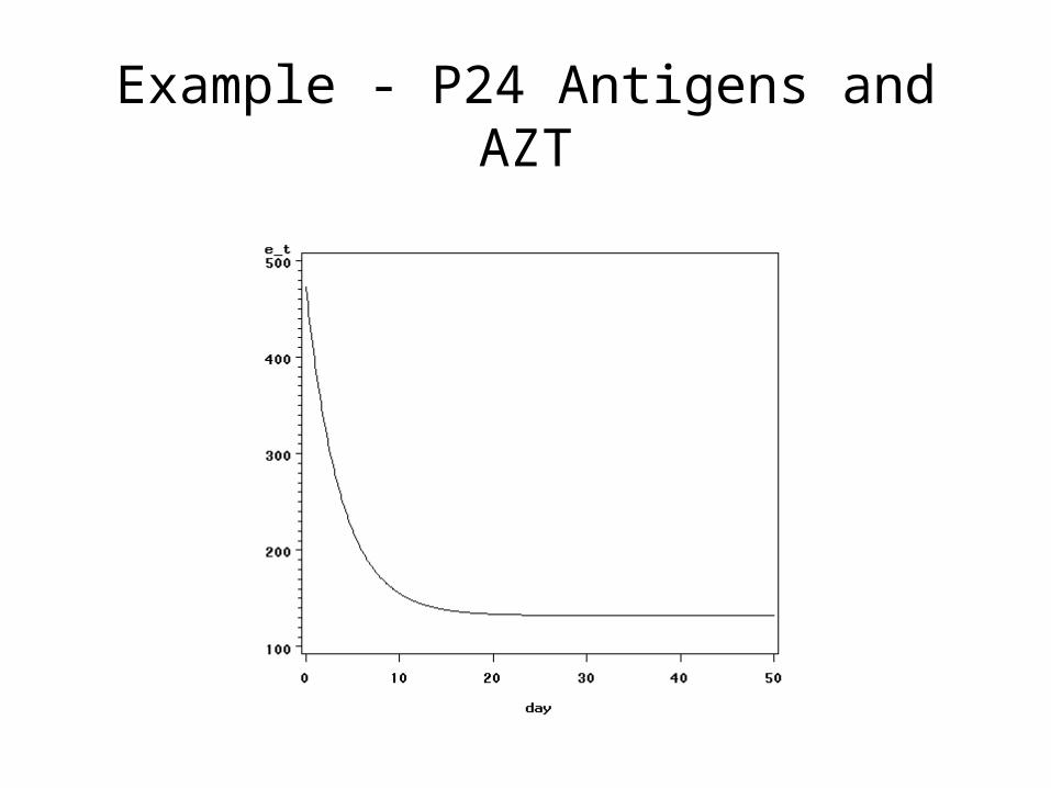
Example - P24 Antigens and AZT
• Goal: Model time course of P24 antigen levels after oral administration of zidovudine
• Model fit individually in 40 HIV+ patients:
AEeAEtE tkout00 )1()(
where:
• E(t) is the antigen level at time t
• E0 is the initial level
• A is the coefficient of reduction of P24 antigen
• kout is the rate constant of decrease of P24 antigen
Source: Sasomsin, et al (2002)

Example - P24 Antigens and AZT
• Among the 40 individuals who the model was fit, the means and standard deviations of the PK “parameters” are given below:
Parameter Mean Std DevE0 472.1 408.8A 0.28 0.21kout 0.27 0.16
• Fitted Model for the “mean subject”
)28.0)(1.472()28.01(1.472)( 27.0 tetE
Example - P24 Antigens and AZT

Example - MK639 in HIV+ Patients
• Response: Y = log10(RNA change)
• Predictor: x = MK639 AUC0-6h
• Model: Sigmoid-Emax:
22
2
1
0
x
xY
• where:
• 0 is the maximum effect (limit as x)
• 1 is the x level producing 50% of maximum effect
• 2 is a parameter effecting the shape of the functionSource: Stein, et al (1996)
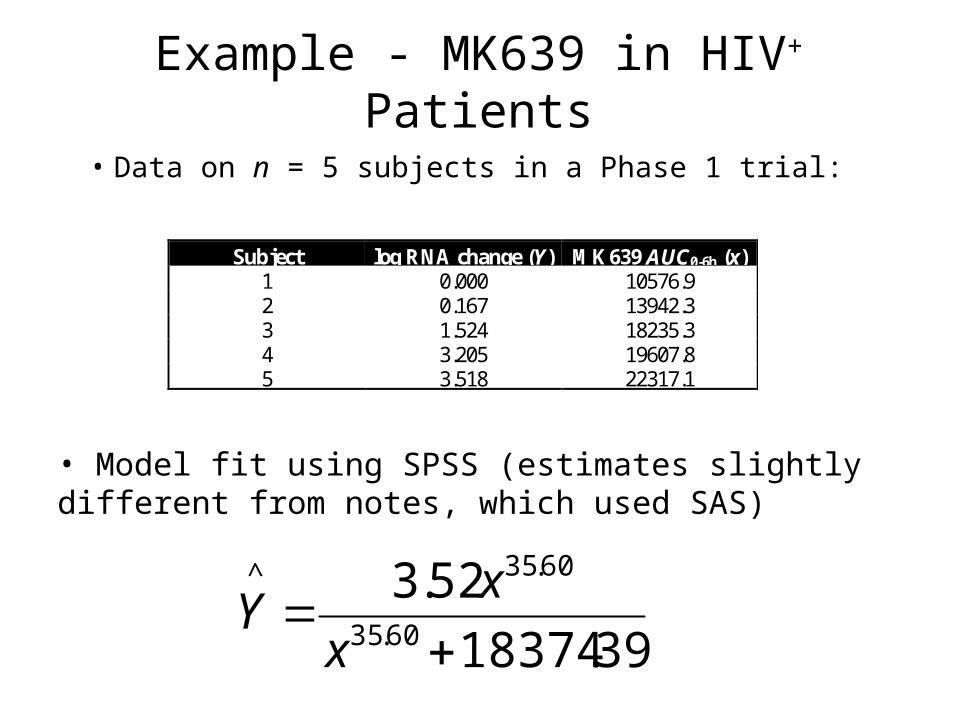
Example - MK639 in HIV+ Patients
• Data on n = 5 subjects in a Phase 1 trial:
Subject log RNA change (Y) MK639 AUC0-6h (x)1 0.000 10576.92 0.167 13942.33 1.524 18235.34 3.205 19607.85 3.518 22317.1
39.18374
52.360.35
60.35^
x
xY
• Model fit using SPSS (estimates slightly different from notes, which used SAS)

Example - MK639 in HIV+ Patients

Data Sources
• Wagner, J.G., G.K. Aghajanian, and O.H. Bing (1968). “Correlation of Performance Test Scores with Tissue Concentration of Lysergic Acid Diethylamide in Human Subjects,” Clinical Pharmacology and Therapeutics, 9:635-638.