Linkage Analysis I-- Parametric

2006.3.3

I-Ping Tu

Book reference

• http://www.math.chalmers.se/Stat/Grundutb/Chalmers/TMS120/kompendium.pdf

• Genetic Linkage Web Resource:

http://linkage.rockefeller.edu/

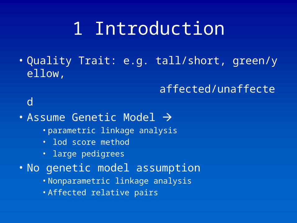
1 Introduction

• Quality Trait: e.g. tall/short, green/yellow,

affected/unaffected

• Assume Genetic Model • parametric linkage analysis• lod score method• large pedigrees

• No genetic model assumption• Nonparametric linkage analysis• Affected relative pairs

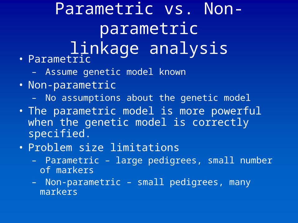
Parametric vs. Non-parametriclinkage analysis

• Parametric– Assume genetic model known

• Non-parametric– No assumptions about the genetic model

• The parametric model is more powerful when the genetic model is correctly specified.

• Problem size limitations– Parametric – large pedigrees, small number of

markers– Non-parametric – small pedigrees, many markers

Phenotype

• Binary– affected or unaffected – Left handed or right handed

• Affected, unaffected, and unknown– Unknown – possibly part of the syndrome

• Quantitative– Insulin resistance – Blood Pressure

Definitions

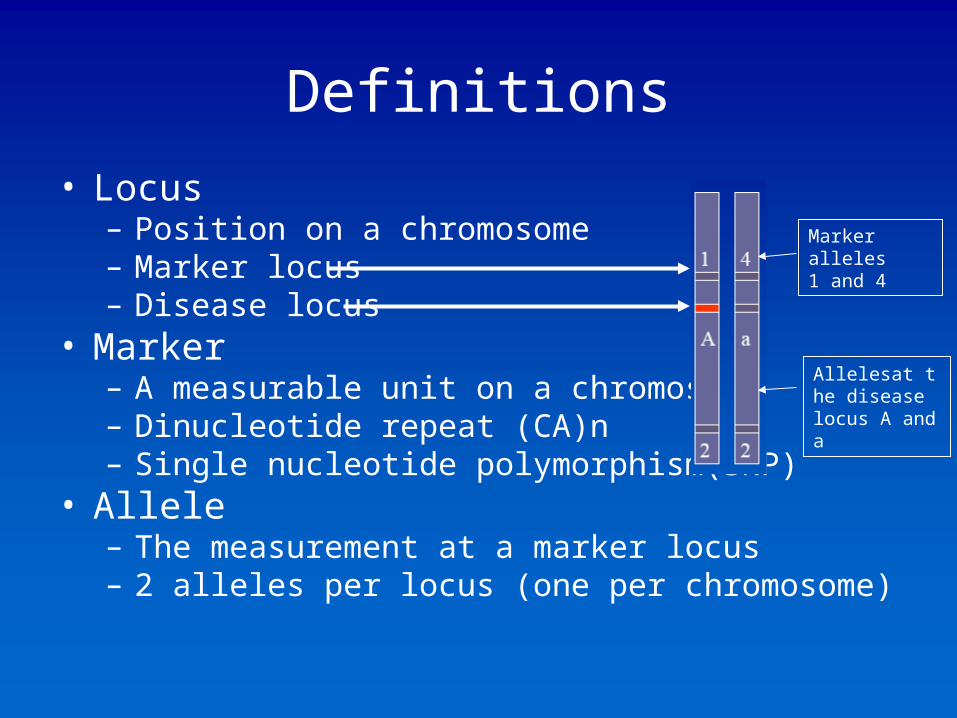
• Locus– Position on a chromosome – Marker locus – Disease locus

• Marker– A measurable unit on a chromosome– Dinucleotide repeat (CA)n– Single nucleotide polymorphism(SNP)

• Allele– The measurement at a marker locus – 2 alleles per locus (one per chromosome)

Marker alleles1 and 4

Allelesat the disease locus A and a

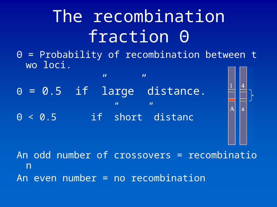
The recombination fraction Θ

Θ = Probability of recombination between two loci.

Θ = 0.5 if ”large” distance.

Θ < 0.5 if ”short” distanc

An odd number of crossovers = recombinationAn even number = no recombination

Haldane’s Mapping function

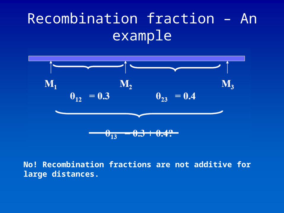
Recombination fraction – An example

No! Recombination fractions are not additive for large distances.

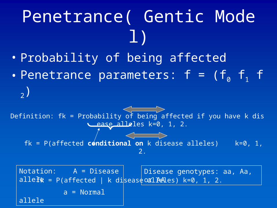
Penetrance( Gentic Model)

• Probability of being affected

• Penetrance parameters: f = (f0 f1 f2)

Definition: fk = Probability of being affected if you have k disease alleles k=0, 1, 2.

fk = P(affected conditional on k disease alleles) k=0, 1, 2.

fk = P(affected | k disease alleles) k=0, 1, 2.

Notation: A = Disease allele

a = Normal allele

Disease genotypes: aa, Aa, or AA

Penetrance continuedRecessive Dominant

Full p. Reduced p. Full p. Reduced p.

f0 = P(aff| aa) 0 0 0 0

f1 = P(aff | Aa) 0 0 1 0.8

f2 = P(aff| AA) 1 0.7 1 0.8

Dominant with

phenocopies and

reduced penetrance Additive penetrances

f0 = 0.01 f0 = 0

f1 = 0.8 f1 = 0.4Age dependent

penetrances f2 = 0.8 f2 = 0.8

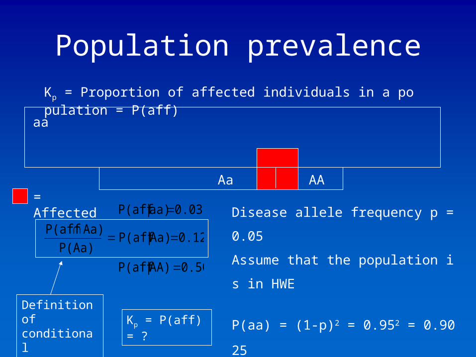
Population prevalence

Kp = Proportion of affected individuals in a population = P(aff)

aa

Aa AA= Affected

0.50 AA) |P(aff

0.12 Aa) |P(aff P(Aa)

Aa)P(aff

0.03 aa) |P(aff

Disease allele frequency p = 0.05

Assume that the population is in HWE

P(aa) = (1-p)2 = 0.952 = 0.9025

P(Aa) = 2p(1-p) =0.095

P(AA) = p2 = 0.0025

Definition of conditional probability

Kp = P(aff) = ?

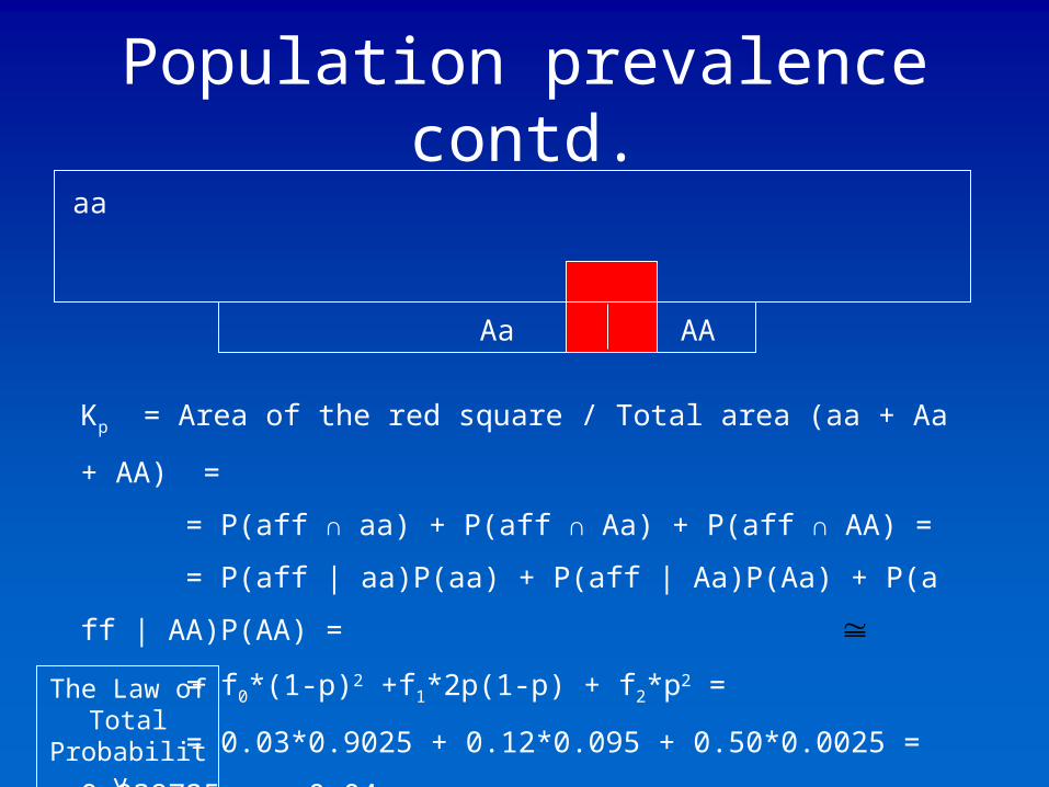
Population prevalence contd.

aa

Aa AA

Kp = Area of the red square / Total area (aa + Aa + AA) =

= P(aff ∩ aa) + P(aff ∩ Aa) + P(aff ∩ AA) =

= P(aff | aa)P(aa) + P(aff | Aa)P(Aa) + P(aff | AA)P(AA) =

= f0*(1-p)2 +f1*2p(1-p) + f2*p2 =

= 0.03*0.9025 + 0.12*0.095 + 0.50*0.0025 = 0.039725 0.04

The Law of Total

Probability

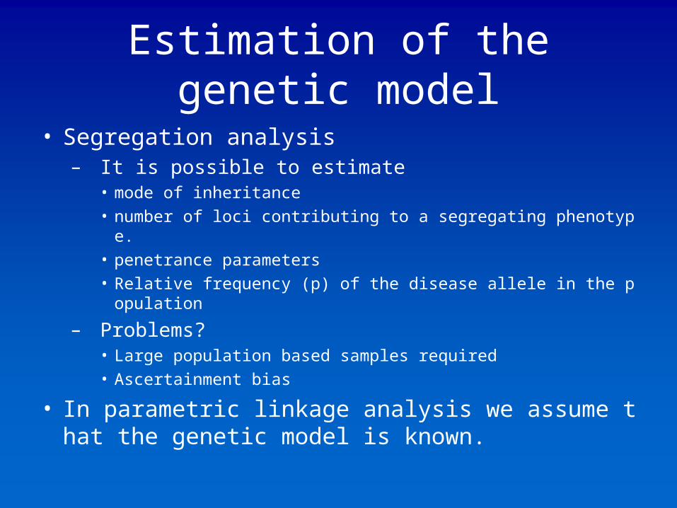
Estimation of the genetic model

• Segregation analysis– It is possible to estimate

• mode of inheritance• number of loci contributing to a segregating phenotype.• penetrance parameters• Relative frequency (p) of the disease allele in the population

– Problems?• Large population based samples required• Ascertainment bias

• In parametric linkage analysis we assume that the genetic model is known.

2. Parametric two-pointlinkage analysis

• Let be the recombination freq between the diseased gene and the observed marker.– H0: = 0.5 VS HA: < 0.5

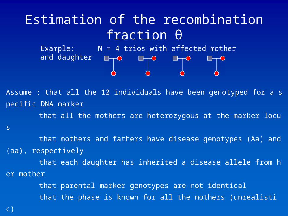
Estimation of the recombination fraction θ

Example: N = 4 trios with affected mother and daughter

Assume : that all the 12 individuals have been genotyped for a specific DNA marker

that all the mothers are heterozygous at the marker locus

that mothers and fathers have disease genotypes (Aa) and (aa), respectively

that each daughter has inherited a disease allele from her mother

that parental marker genotypes are not identical

that the phase is known for all the mothers (unrealistic)

Data : Trio 1-3: No recombination between marker and disease locus

Trio 4: Recombination between marker and disease locus

Estimate : θ* = 1/4

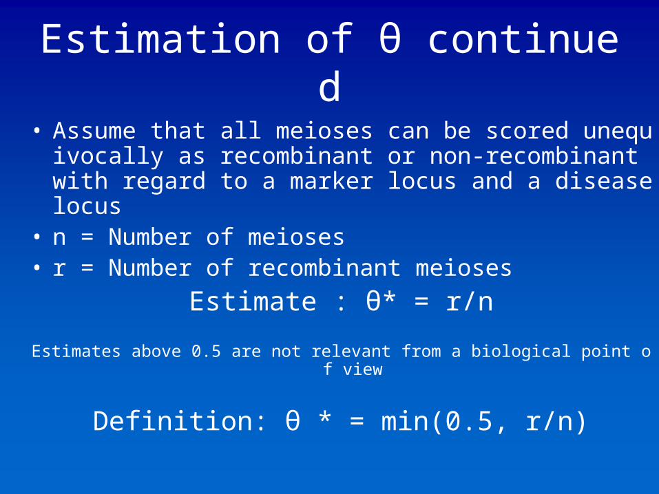
Estimation of θ continued

• Assume that all meioses can be scored unequivocally as recombinant or non-recombinant with regard to a marker locus and a disease locus

• n = Number of meioses• r = Number of recombinant meioses

Estimate : θ* = r/n

Estimates above 0.5 are not relevant from a biological point of view

Definition: θ * = min(0.5, r/n)

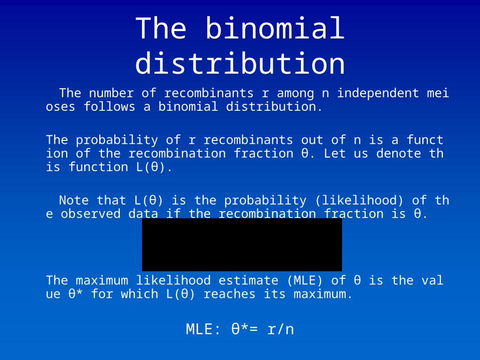
The binomial distribution

The number of recombinants r among n independent meioses follows a binomial distribution.

The probability of r recombinants out of n is a function of the recombination fraction θ. Let us denote this function L(θ).

Note that L(θ) is the probability (likelihood) of the observed data if the recombination fraction is θ.

The maximum likelihood estimate (MLE) of θ is the value θ* for which L(θ) reaches its maximum.

MLE: θ*= r/n

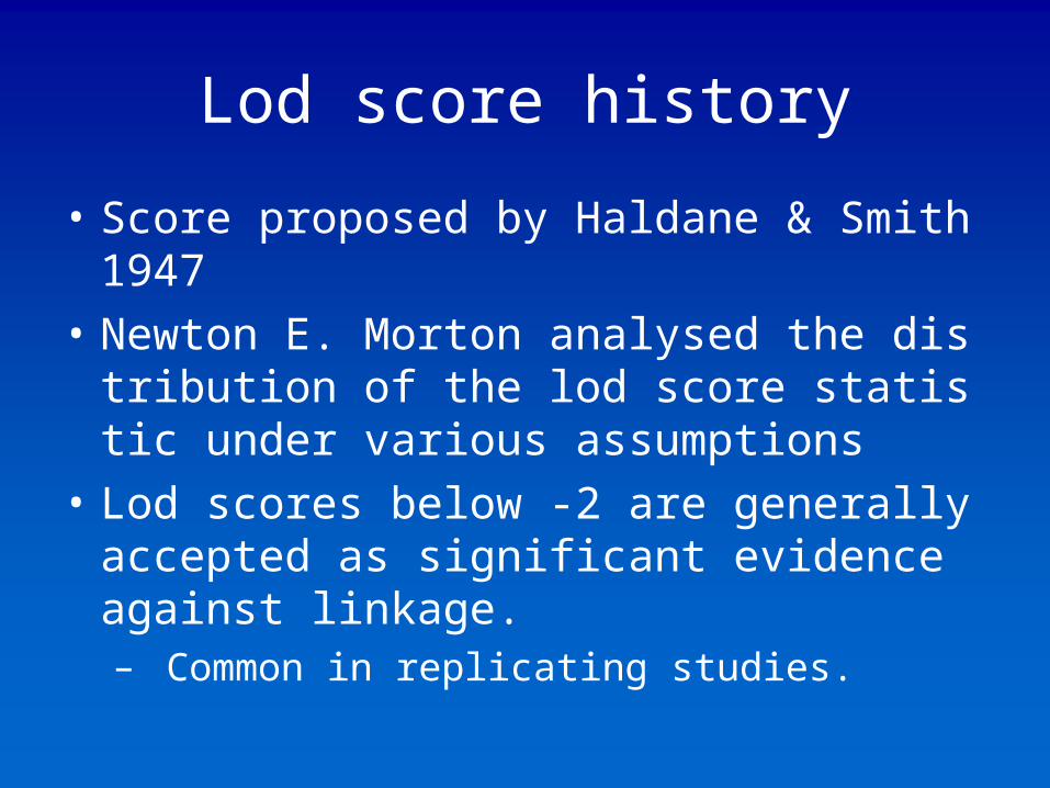
Lod score history

• Score proposed by Haldane & Smith 1947

• Newton E. Morton analysed the distribution of the lod score statistic under various assumptions

• Lod scores below -2 are generally accepted as significant evidence against linkage.– Common in replicating studies.

0

0

0

10

11

11A010

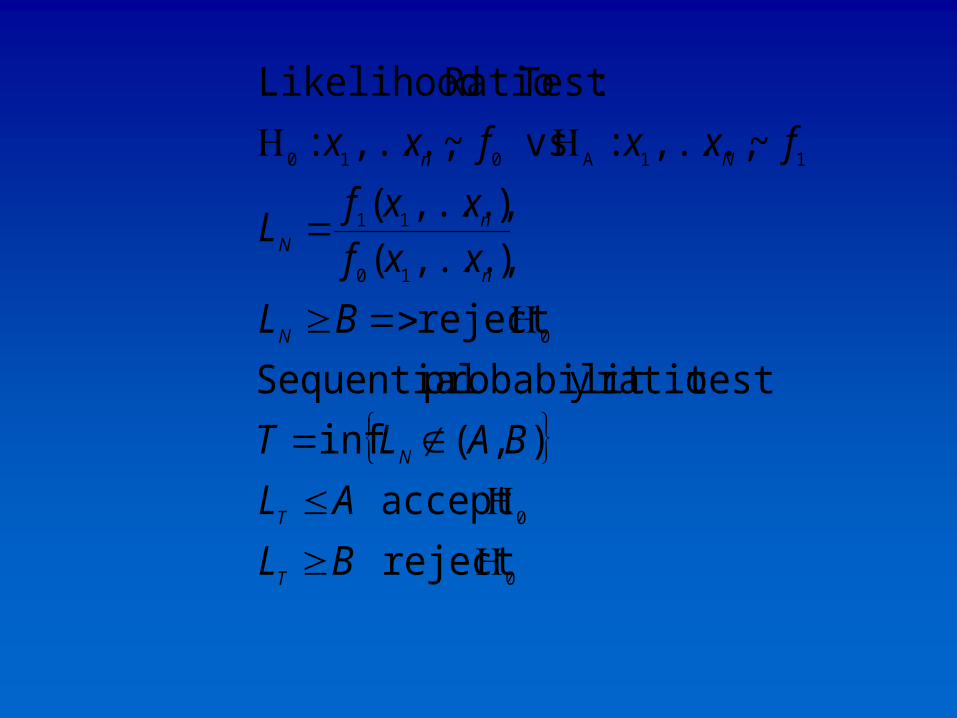
reject

accept

),(inf

testratioy probabilit Sequential

reject

),...,(

),...,(

~,...,: vs~,...,:

:Test RatioLikelihood

BL

AL

BALT

BL

xxf

xxfL

fxxfxx

T

T

N

N

n

nN

Nn

BA

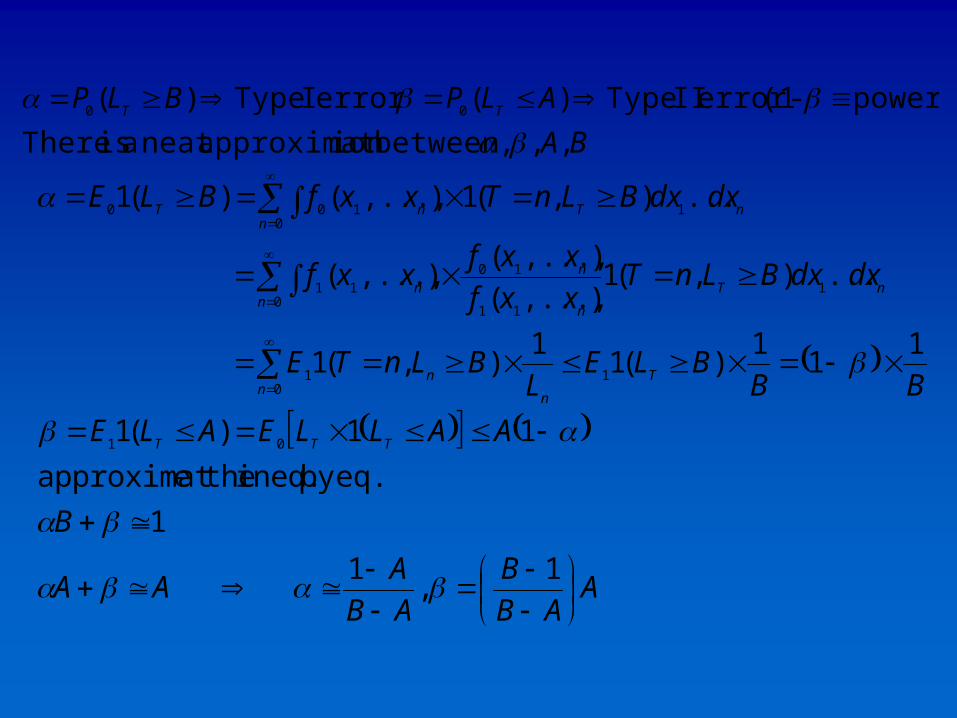
ALPBLP TT

,,, between ionapproximatneat a is There

power)-(1error II Type )(error I Type)( 00

AAB

B

AB

AAA

B

AALLEALE

BBBLE

LBLnTE

dxdxBLnTxxf

xxfxxf

dxdxBLnTxxfBLE

TTT

Tn

n

n

nnT

n

nn

nnTnT

1,

1

1

eq.by ineq. theeapproximat

11)(1

11

1)(1

1),(1

...),(1),...,(

),...,(),...,(

...),(1),...,()(1

01

10

1

01

11

1011

01100

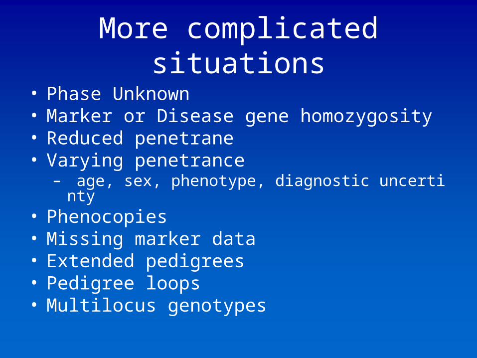
More complicated situations

• Phase Unknown• Marker or Disease gene homozygosity• Reduced penetrane• Varying penetrance

– age, sex, phenotype, diagnostic uncertinty• Phenocopies• Missing marker data• Extended pedigrees• Pedigree loops• Multilocus genotypes

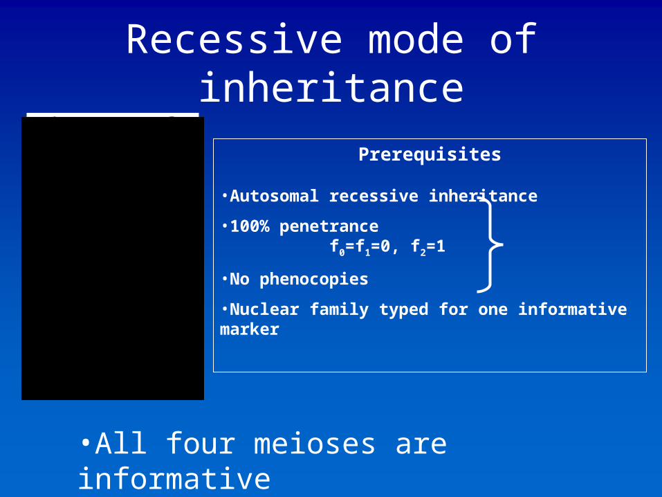
Recessive mode of inheritance

Prerequisites

•Autosomal recessive inheritance

•100% penetrance f0=f1=0, f2=1

•No phenocopies

•Nuclear family typed for one informative marker

•All four meioses are informative

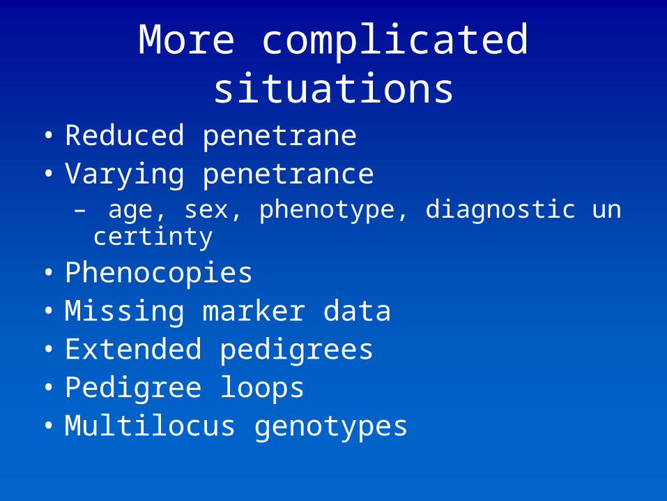
More complicated situations

• Reduced penetrane• Varying penetrance

– age, sex, phenotype, diagnostic uncertinty

• Phenocopies• Missing marker data• Extended pedigrees• Pedigree loops• Multilocus genotypes

Lod score assignment

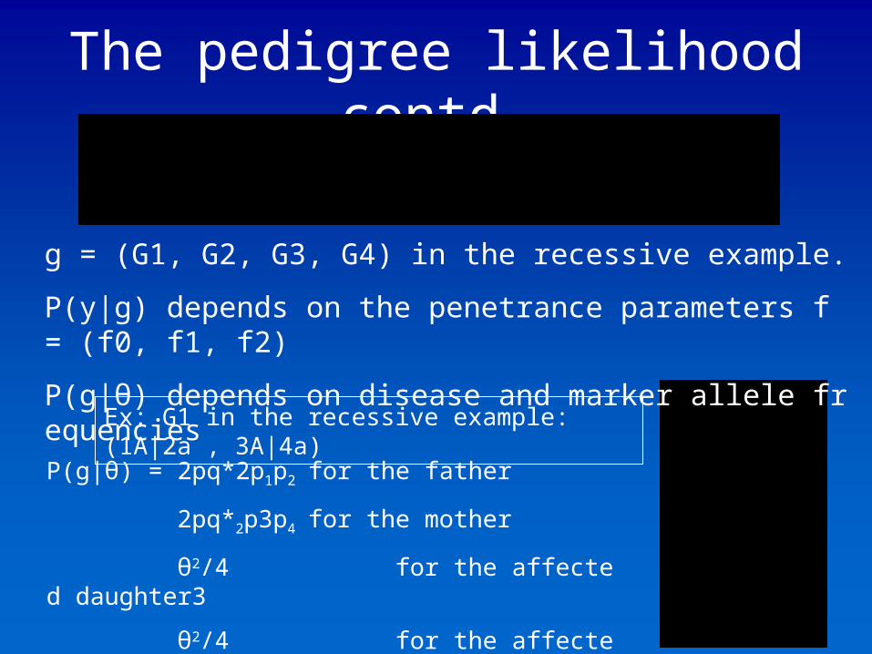
The pedigree likelihood contd.

g = (G1, G2, G3, G4) in the recessive example.

P(y|g) depends on the penetrance parameters f = (f0, f1, f2)

P(g|θ) depends on disease and marker allele frequencies

Ex: G1 in the recessive example: (1A|2a , 3A|4a)

P(g|θ) = 2pq*2p1p2 for the father

2pq*2p3p4 for the mother

θ2/4 for the affected daughter3

θ2/4 for the affecteddaughter4

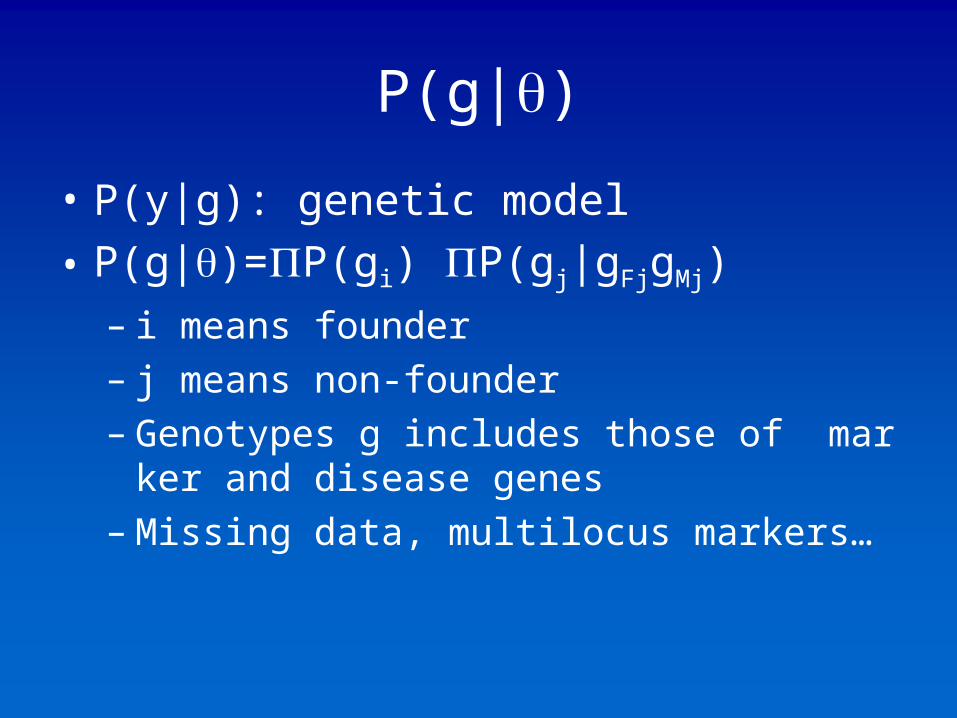
P(g|)

• P(y|g): genetic model

• P(g|)=P(gi) P(gj|gFjgMj)

– i means founder– j means non-founder– Genotypes g includes those of marker and di

sease genes – Missing data, multilocus markers…

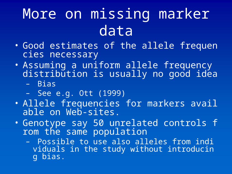
More on missing marker data

• Good estimates of the allele frequencies necessary

• Assuming a uniform allele frequency distribution is usually no good idea– Bias– See e.g. Ott (1999)

• Allele frequencies for markers available on Web-sites.

• Genotype say 50 unrelated controls from the same population– Possible to use also alleles from individuals in the stu

dy without introducing bias.

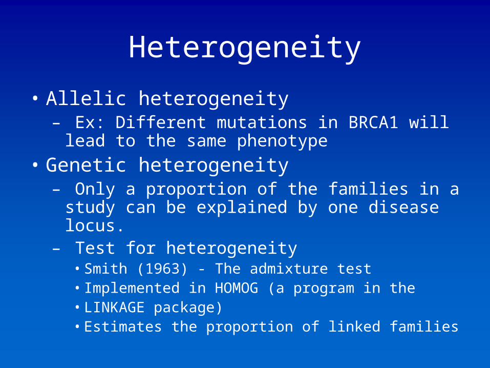
Heterogeneity

• Allelic heterogeneity– Ex: Different mutations in BRCA1 will lead to

the same phenotype

• Genetic heterogeneity– Only a proportion of the families in a study

can be explained by one disease locus.– Test for heterogeneity

• Smith (1963) - The admixture test• Implemented in HOMOG (a program in the• LINKAGE package)• Estimates the proportion of linked families

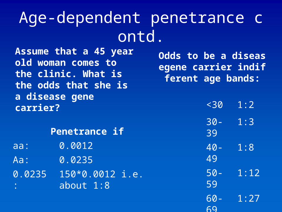
Age-dependent penetrance contd.

Assume that a 45 year old woman comes to the clinic. What is the odds that she is a disease gene carrier?

Odds to be a diseasegene carrier indifferent ag

e bands:

Penetrance if

aa: 0.0012

Aa: 0.0235

0.0235 : 150*0.0012 i.e. about 1:8

<30 1:2

30-39 1:3

40-49 1:8

50-59 1:12

60-69 1:27

70-79 1:36

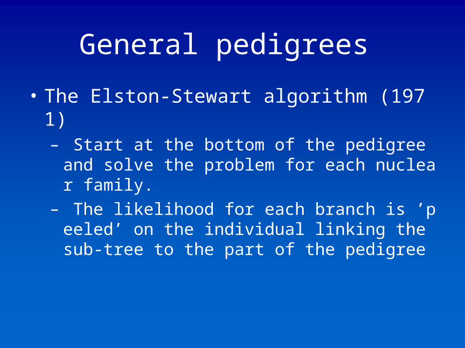
General pedigrees

• The Elston-Stewart algorithm (1971)– Start at the bottom of the pedigree and solve

the problem for each nuclear family.– The likelihood for each branch is ’peeled’ on t

he individual linking the sub-tree to the part of the pedigree

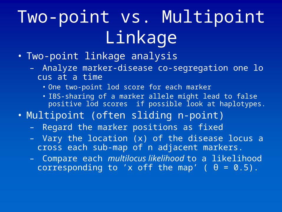
Two-point vs. Multipoint Linkage

• Two-point linkage analysis– Analyze marker-disease co-segregation one locus at

a time• One two-point lod score for each marker• IBS-sharing of a marker allele might lead to false positive lod

scores if possible look at haplotypes.

• Multipoint (often sliding n-point)– Regard the marker positions as fixed– Vary the location (x) of the disease locus across each

sub-map of n adjacent markers.– Compare each multilocus likelihood to a likelihood co

rresponding to ’x off the map’ ( θ = 0.5).

Software

• Jurg Otts website at Rockefeller University– http://linkage.rockefeller.edu/soft

• For parametric linkage analysis– LINKAGE– FASTLINK– VITESSE

Linkage Analysis II--Nonparametric

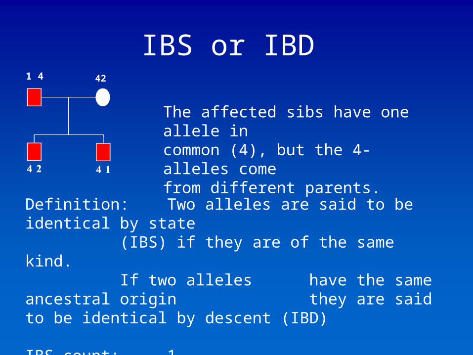
IBS or IBD 1 4 42

The affected sibs have one allele incommon (4), but the 4-alleles comefrom different parents.

Definition: Two alleles are said to be identical by state(IBS) if they are of the same kind. If two alleles have the same ancestral origin

they are said to be identical by descent (IBD)

IBS-count: 1IBS is a weaker concept than IBD

IBD-count: 0

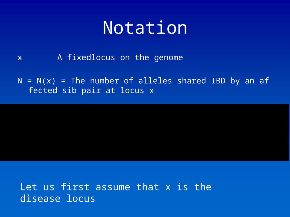
Notation

x A fixedlocus on the genome

N = N(x) = The number of alleles shared IBD by an affected sib pair at locus x

Let us first assume that x is the disease locus

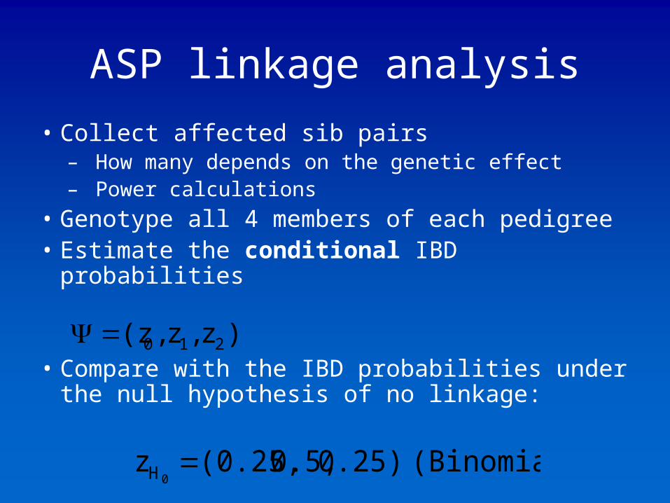
ASP linkage analysis

• Collect affected sib pairs– How many depends on the genetic effect– Power calculations

• Genotype all 4 members of each pedigree• Estimate the conditional IBD probabilities

• Compare with the IBD probabilities under the null hypothesis of no linkage:

)z ,z ,(z 210

(Binomial) 0.25) 0.5, (0.25, z 0H

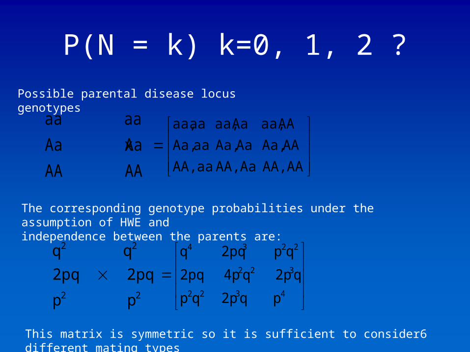
P(N = k) k=0, 1, 2 ?

Possible parental disease locus genotypes

AA AA

Aa x Aa

aa aa

AAAA, AaAA, aaAA,

AAAa, AaAa, aaAa,

AAaa, Aaaa, aaaa,

The corresponding genotype probabilities under the assumption of HWE andindependence between the parents are:

22

22

p p

2pq 2pq

q q

4322

322

223 4

p q2p qp

q2p q4p 2pq

qp 2pq q

This matrix is symmetric so it is sufficient to consider6 different mating types

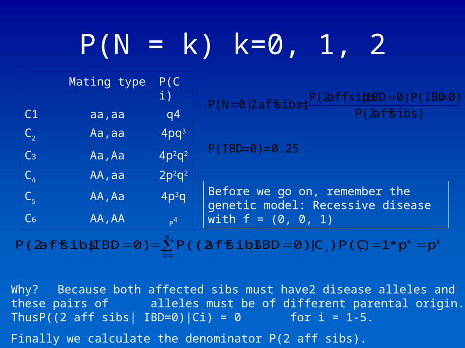
P(N = k) k=0, 1, 2Mating type P(Ci)

C1 aa,aa q4

C2 Aa,aa 4pq3

C3 Aa,Aa 4p2q2

C4 AA,aa 2p2q2

C5 AA,Aa 4p3q

C6 AA,AA P4

0.250)P(IBD

sibs) aff P(2

0)0)P(IBDIBD |affsibs P(2 sibs) aff 2 | 0P(N

Before we go on, remember the genetic model: Recessive disease with f = (0, 0, 1)

446

1iii pp*1))P(CC|0)IBDsibs aff P((20)IBD |sibs aff P(2

Why? Because both affected sibs must have2 disease alleles and these pairs of alleles must be of different parental origin. ThusP((2 aff sibs| IBD=0)|Ci) = 0 for i = 1-5.

Finally we calculate the denominator P(2 aff sibs).

IBD probabilities for a few genetic modelsTable 2.1 page 30 in the compendium

λs= Sibling relative risk = 0.25/z0 (strength of the genetic component)

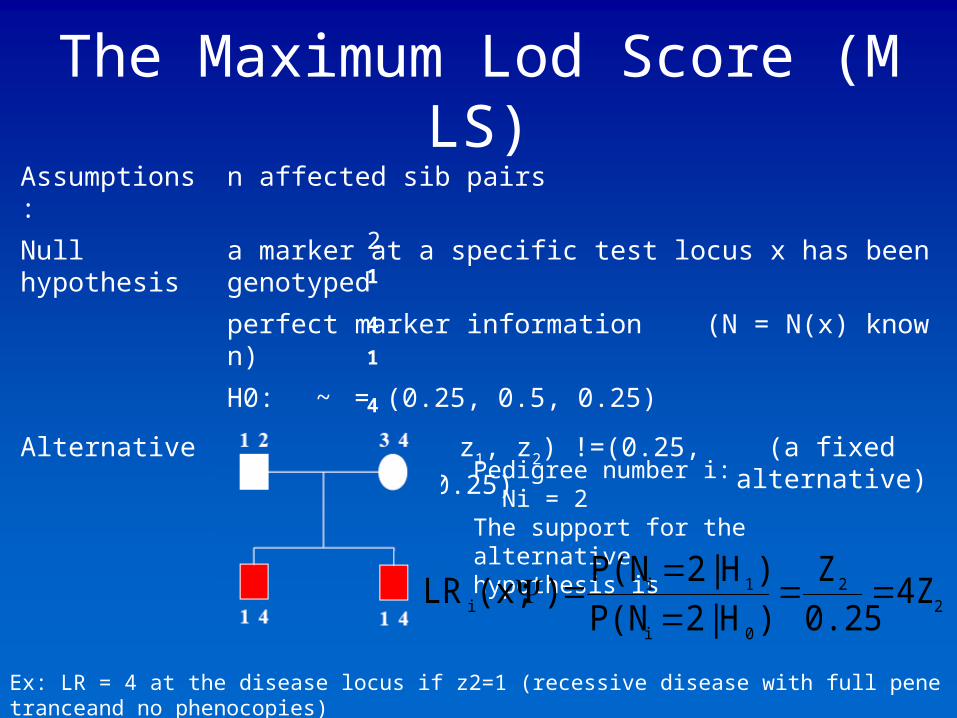
The Maximum Lod Score (MLS)Assumptions: n affected sib pairs

Null hypothesis a marker at a specific test locus x has been genotyped

perfect marker information (N = N(x) known)

H0: ~ = (0.25, 0.5, 0.25)

Alternative H1: ~ = (z0, z1, z2) !=(0.25, 0.5, 0.25) (a fixed alternative)

2

1 4

1 4

Pedigree number i: Ni = 2The support for the alternativehypothesis is

Ex: LR = 4 at the disease locus if z2=1 (recessive disease with full penetranceand no phenocopies)

22

0i

1ii 4Z

0.25

Z

)H|2P(N

)H|2P(N)(x;LR

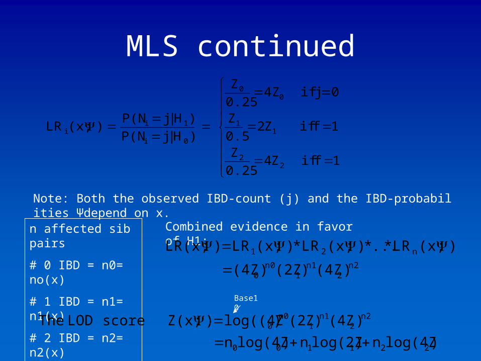
MLS continued

1f if Z40.25

Z

1f if Z20.5

Z

0j if 4Z0.25

Z

)H|jP(N

)H|jP(N )(x;LR

22

11

00

0i

1ii

Note: Both the observed IBD-count (j) and the IBD-probabilities Ψdepend on x.

n affected sib pairs

# 0 IBD = n0= no(x)

# 1 IBD = n1= n1(x)

# 2 IBD = n2= n2(x)

Combined evidence in favor of H1:

n22

n11

n00

n21

)(4Z)(2Z)(4Z

)(x;LR* ...* )(x;LR* )(x;LR )LR(x;

)log(4Zn)log(2Zn )log(4Zn

)(4Z)(2Z)log((4Z )Z(x; score LOD The

221100

n22

n11

n00

Base10

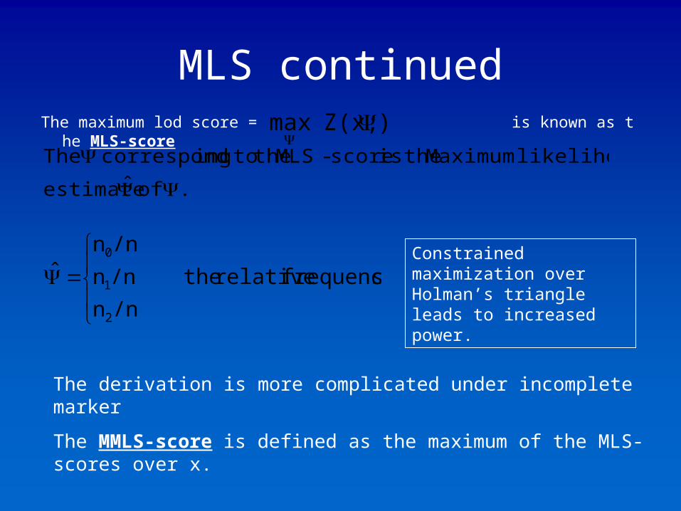
MLS continuedThe maximum lod score = is known as the MLS-score) Z(x;max

. of ˆ estimate

likelihood Maximum theis score-MLS the toingcorrespond The

sfrequencie relative the

/nn

/nn

/nn

ˆ

2

1

0

Constrained maximization over Holman’s triangle leads to increased power.

The derivation is more complicated under incomplete marker

The MMLS-score is defined as the maximum of the MLS-scores over x.

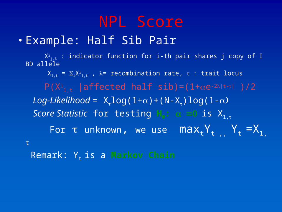
NPL Score• Example: Half Sib Pair Xi

j,t : indicator function for i-th pair shares j copy of IBD allele

X1,t = iXi1,t , = recombination rate, : trait locus

P(Xi1,t |affected half sib)=(1+e-2|t-| )/2

Log-Likelihood = Xlog(1+)+(N-X)log(1- Score Statistic for testing H0: is X1,

For unknown, we use maxtYt ,, Yt =X1,t

Remark: Yt is a Markov Chain

The NPL Score

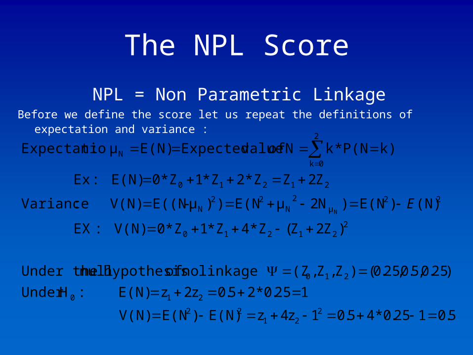
NPL = Non Parametric LinkageBefore we define the score let us repeat the definitions of expectation and variance :

5.0125.0*45.01z4zE(N))E(N V(N)

125.0*25.0z2zE(N) :HUnder

)25.0,5.0,25.0()Z,Z,(Z linkage no of hypothesis null Under the

)Z2Z(Z*4Z*1 Z*0 V(N) :EX

(N))E(N)N2μE(N ))μ-E((N V(N) : Variance

Z2ZZ*2Z*1 Z*0 E(N) :Ex

k)P(N*k N of valueExpected E(N)μ :nExpectatio

221

22

210

210

221210

22μ

2N

22N

21210

2

0kN

N

E

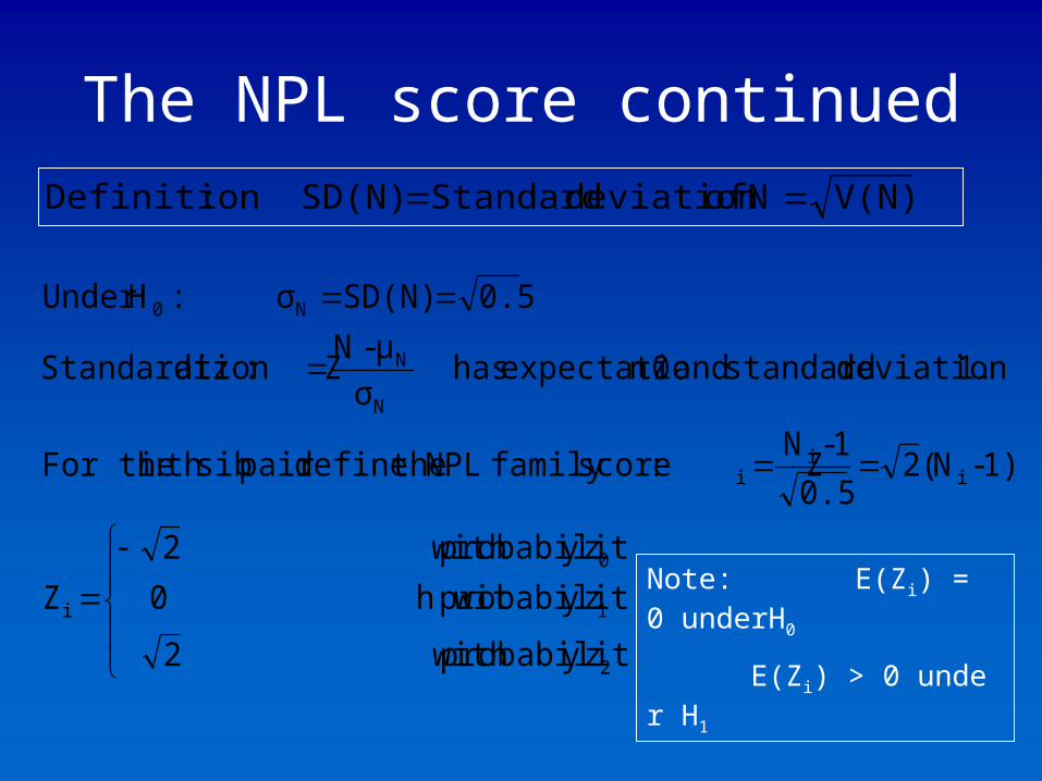
The NPL score continued V(N)N ofdeviation StandardSD(N) :Definition

2

1

0

i

ii

i

N

N

N0

zy probabilit with 2

zy probabilith wit 0

zy probabilit with 2

Z

1)-N(2 0.5

1-N Z:scorefamily NPL thedefinepair sibth :i For the

1.deviation standard and 0n expectatio has σ

μ-N Z:ation Standardiz

0.5SD(N)σ :HUnder

Note: E(Zi) = 0 underH0

E(Zi) > 0 under H1

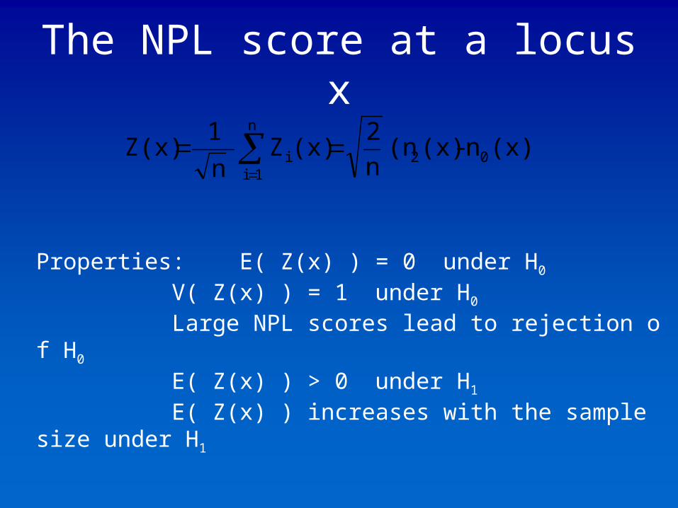
The NPL score at a locus x

(x))n-(x)(n n

2(x)Z

n

1 Z(x) 02

n

1ii

Properties: E( Z(x) ) = 0 under H0

V( Z(x) ) = 1 under H0

Large NPL scores lead to rejection of H0

E( Z(x) ) > 0 under H1

E( Z(x) ) increases with the sample size under H1