Linköping University Electronic Press   

Report

  

  

  

  

Modeling and Experiment Design for Identification of Wear in a Robot Joint under Load and Temperature Uncertainties based on

Constant-speed Friction Data     

André Carvalho Bittencourt and Patrik Axelsson                             

Series: LiTH-ISY-R, ISSN 1400-3902, No. 2058 ISRN: LiTH-ISY-R-3058

  

Available at: Linköping University Electronic Press http://urn.kb.se/resolve?urn=urn:nbn:se:liu:diva-90023

 

Technical report from Automatic Control at Linköpings universitet

Modeling and Experiment Design forIdentification of Wear in a Robot Jointunder Load and TemperatureUncertainties based on Constant-speedFriction Data

André Carvalho Bittencourt, PAtrik AcelssonDivision of Automatic ControlE-mail: andrecb@isy.liu.se, axelsson@isy.liu.se

15th March 2013

Report no.: LiTH-ISY-R-3058Submitted to IEEE-ASME Trans. on Mechatronics

Address:Department of Electrical EngineeringLinköpings universitetSE-581 83 Linköping, Sweden

WWW: http://www.control.isy.liu.se

AUTOMATIC CONTROLREGLERTEKNIK

LINKÖPINGS UNIVERSITET

Technical reports from the Automatic Control group in Linköping are available fromhttp://www.control.isy.liu.se/publications.

Abstract

The e�ects of wear to friction are studied based on constant-speed friction

data collected from dedicated experiments during accelerated wear tests.

It is shown how the e�ects of temperature and load uncertainties produce

larger changes to friction than those caused by wear, motivating the con-

sideration of these e�ects. Based on empirical observations, an extended

friction model is proposed to describe the e�ects of speed, load, temper-

ature and wear. Assuming availability of such model and constant-speed

friction data, a maximum likelihood wear estimator is proposed. A crite-

rion for experiment design is proposed which selects speed points to collect

constant-speed friction data which improves the achievable performance

bound for any unbiased wear estimator. Practical issues related to exper-

iment length are also considered. The performance of the wear estimator

under load and temperature uncertainties is found by means of simulations

and veri�ed under three case studies based on real data.

Keywords: industrial robotics, wear, friction, identi�cation, condition mon-

itoring

1

Modeling and Experiment Design for Identificationof Wear in a Robot Joint under Load and

Temperature Uncertainties based on Constant-speedFriction Data

Andre Carvalho Bittencourt and Patrik Axelsson

Abstract—The wear effects to friction are studied based onconstant-speed friction data collected from dedicated experimentsduring accelerated wear tests. It is shown how the effects oftemperature and load uncertainties produce larger changes tofriction than those caused by wear, motivating the considerationof these effects. Based on empirical observations, an extendedfriction model is proposed to describe the effects of speed, load,temperature and wear. Assuming availability of such modeland constant-speed friction data, a maximum likelihood wearestimator is proposed. A criterion for experiment design isproposed which selects speed points to collect constant-speedfriction data which improves the achievable performance boundfor any unbiased wear estimator. Practical issues related toexperiment length are also considered. The performance of thewear estimator under load and temperature uncertainties isfound by means of simulations and verified under three casestudies based on real data.

Index Terms—industrial robotics, wear, friction, identification,condition monitoring

I. INTRODUCTION

FRICTION can be defined as the tangential reaction forcebetween two surfaces in contact. It is not a fundamental

force but the result of complex interactions between contactingsurfaces down to a nanoscale perspective. Friction alwaysopposes motion, dissipating kinetic energy. A part of thework produced by friction appears as heat transfer, vibrationsand acoustic emissions. Other outcomes of friction are dueto mechanical action between the surfaces, such as plasticdeformation, adhesion and fracture. The later are related towear, which can be defined as “the progressive loss of materialfrom the operating surface of a body occurring as a resultof relative motion at its surface” (quoted from [1]). Theneed for relative motion between surfaces implies that thewear mechanisms are related tomechanicalaction betweensurfaces. This is an important distinction to other processeswith a similar outcome and very different nature, e.g. corrosion(see [2] for basics on wear related phenomena).

Excessive wear may lead to a deterioration of the system’sperformance and to an eventual failure. The potential damagescaused by excessive wear can however be prevented if goodmaintenance practices are performed. In order to support

The authors are with the Department of Electrical Engineering, LinkopingsUniversity, Linkoping, Sweden.{andrecb, axelsson}@isy.liu.se

This work was supported by ABB and the Vinnova Industry ExcellenceCenter LINK-SIC at Linkoping University.

maintenance actions, the use of methods to determine thecondition of the equipment is desirable, allowing for condition-based maintenance (CBM). The wear processes inside a robotjoint cause an eventual increase of wear debris in the lubricant.Monitoring the iron content of lubricant samples taken fromthe robot joint can thus be used as an indication of the jointcondition. The study of wear debris particles is known asferrography and was first introduced in [3]. Since then, thescience has evolved and helped to understand wear relatedphenomena (see [4] for a historical review on ferrography).These techniques are however intrusive and costly, requiringlaboratory analyses and alternatives which do not rely onadditional sensory information are preferred.

The accumulated wear in a tribosystem may lead to varia-tions in friction (see [5] for a review on the relation betweenwear and friction). As shown by experimental studies inthis paper, such relation is also present for a robot joint.Alternatives for wear monitoring are thus possible provided itis possible toobserve frictionand the relation betweenfrictionand wear is known. Monitoring friction to infer about wearis however challenging since friction is significantly affectedby other factors than wear such as temperature and load (seeFig. 3). The effects of temperature are specially difficult sincetemperature is not measured in typical robot applications.These co-effects should nevertheless be considered when ver-ifying the reliability of a solution.

In the literature , little can be found about wear estimationfor industrial robots. This may be attributed to the lack ofwear models available and the high costs and time required toperform wear experiments. There are related approaches usedfor fault detection, where the objective is to decide whethera change from nominal is present. In the related literature,faults are typically consider as actuator malfunctions, modeledas changes in the output torque signals or in parameters of arobot model, including the case offriction changes, which isimportant since they can relate to wear.

Theestimation of friction parametersin a robot model frommeasured data is a natural approach for fault detection becauseof their physical interpretation. A shortcoming is the needforexcitation in the data, which might be restricting in some appli-cations. In [6], a least-squares method is used to estimate robotparameters over a moving window. Estimates of the Coulomband viscous friction parameters are compared to confidence

2

values of their nominal behavior for fault detection. In thepaper, an experimental study is shown where the estimatedfriction parameters could indicate some of the faults but couldnot readily distinguish between them, e.g. the increase of jointtemperature had a similar effect as a fault in the drive-chain.

Monitoring estimates of the Coulomb and viscous param-eters is also considered in [7]. The parameters are estimatedfrom constant-speed friction data collected from experimentsin an off-line manner, using a procedure similar to what isused in this paper (see Sec. II-A). These data are collected fordifferent speed levels, forming a so-calledfriction curve (seee.g. Fig. 3 for examples of friction curves). In [7], the areaunder the friction curve is also monitored, which is relatedto the energy needed to overcome friction, i.e. a “frictioncurve energy”. Experimental work suggested that monitoringthe Coulomb and/or viscous friction parameters are not robustsolutions to detect wear changes even under rather constantload and temperature conditions. The use of the friction curveenergy improved the robustness, but as it was shown (compareFig. 6.3(d) with Fig. A.1 in [7]) it still cannot distinguishfromthe effects of temperature. Its behavior was also found to bedependent on properties of the lubricant used. As illustratedhere, the effects of wear and temperature affect friction ina similar manner and the simple friction model used in [6],[7] did not consider these effects. As it will be shown, theuse of a more detailed friction model allows for a reliableestimation of the effects of wear even under temperature andload uncertainties.

Estimates of the viscous friction parameter were also con-sidered in [8] to monitor the lubricant health in a mechanicaltransmission. The parameter estimates are achieved based onthe energy balance for the system over a time window. As itis shown in experiments, changes in the lubricant viscositycan be monitored by comparison of the estimated viscousparameter with that generated by a model. Because viscousfriction is highly dependent on the lubricant temperature,atemperature-dependent model is used. The lubricant tempera-ture is estimated based on a Kalman filter using environmenttemperature measurements and a heat transfer model. A similarapproach but based on an observer of the viscous frictiontorque is also presented in [9] with simulation studies for arobot joint.

Considering the nonlinear nature of a manipulator, the useof nonlinear observersis another common approach for faultdetection, see e.g. [10], [11]. Different design approaches areused and the observer stability is typically guaranteed byanalyses of the decay rate of a candidate Lyapunov function.Due to uncertainties in the modeling assumptions, approacheshave been suggested to improve robustness. In [12]–[14],nonlinear observers are used together with adaptive schemeswhile in [15] support vector machines are trained to model theuncertainties. In [16], a nonlinear fault observer is suggestedbased on a neural network model for the abnormal robotbehavior and defines a robust adaptation rule based on knownuncertainties’ bounds. In [13], [17], the residuals of a nonlinearobserver of generalized momenta are used for detection ofactuator faults, the derivation of such observer is rather simpleand compared to [18], where the residuals of a torque observer

are used, it does not require inversion of the inertia matrix;an efficient implementation for the former is also discussedin [19].

The use of unknown input (fault) observers, as presentedin [11], [16], is important to support, e.g., control law re-configuration and diagnosis. In [20], an extended Kalman-Bucy filter is used to estimate friction torques in a rotatingmachine; the presence of a friction change is detected basedona multiple hypotheses test in a Bayesian framework where eachhypothesis is associated to a known friction model. A frictionobserver for control is also suggested in [21] using joint torquemeasurements; the observer is inspired by the generalizedmomenta observer presented in [13], [17], its structure is of alinear low-pass filter of the actual friction torque.

While observer design is mainly dependent on a robotmodel, observers can also be achieved by direct processingof input-output data, where a black-box model is identifiedto provide estimates of measured signals. The use ofneuralnetworkand neuro-fuzzy models are common, see e.g. [22],[23], but also support vector machines have been consid-ered [24]. Disadvantages of these methods are the need fortraining data and the difficulties in guaranteeing their gener-alization capacities, with a compromise between adaptationand detection performance. Similar approaches can be usedfor fault classification, requiring faulty data for the trainingstage, which is difficult in practice; see [25] for a review ofindustrial use of neural networks.

Less studied for nonlinear systems areparity-spaceap-proaches, where a model of the system is used to find aprojection of the input-output data to a space dependent onfaults and errors but not on the states. In [26], the authorspropose a projection which is robust to modeling errors andnoise. Practical difficulties with such approaches for nonlinearsystems is the need for higher order derivatives of the inputand output data and high computational complexity. Note thatwhile parity spaces and observers are equivalent for linearsystems (as shown in [27]), this is not the case for nonlinearsystems (see the discussion in [28]).

In [29], the passivity property of Lagrangian systems isused to defineenergy balanceequations which are monitoredfor fault detection and isolation; the framework is illustratedwith a simulation study of a robot manipulator with faultsin dissipative components (e.g. friction changes) and energy-storing components (e.g. load changes). As advantages toclassical methods, the author mentions the simplicity of themodels used in an energy model compared to, e.g., modelsused for nonlinear observers, and the low complexity foron-line implementation. Because the energy balance is alsoaffected by disturbances, knowledge of these effects to thesystem’s energy can be used to achieve robustness; someapproaches are discussed in [29]. In [30], the energy balance iscomputed over a moving window to perform fault diagnosis ina robotic system. A known robot model is considered availableand thresholds are determined based on available bounds onthe model uncertainties, allowing for fault detection. Faultisolation and identification are achieved based on investigationof the correlation of the residuals to multiple fault energypatterns. A simulation study illustrates the framework, where

3

actuator faults are successfully diagnosed; the case of con-comitant faults is also illustrated.

The vibration patternsgenerated from a robot joint alsocontain valuable information about its condition. In [31],neural networks are used to learn the vibration patterns of arobot based on accelerometers’ measurements. Similarly, theacoustic emissions of the robot joints may change under afault. In [32], features of sound measurements, i.e. peaks of awavelet transformation, are monitored and determination of afault is done based on labeled data using a nearest neighborclassifier. Besides the extra sensors needed, these approachesrequire data from a pre-defined trajectory which makes themunsuitable for on-line monitoring.

In this paper, a wear estimator is proposed based on a knownfriction model and constant-speed friction data which areachieved throughdedicated experiments, in an off-line manner.A solution based on a dedicated experiment will decrease therobot availability which is undesired from the perspectiveofa robot user. The trade-off between experiment length andthe estimator accuracy is therefore important and is studiedin detail. Themain contributions leading to the proposedsolution are listed

• first, the effects of wear to friction are modeled based onempirical observations;

• an extended friction model is proposed and identifiedthat describes the effects of speed, temperature, load andwear;

• experiment design is considered based on the achievableperformance for any unbiased wear estimator;

• with a known friction model, a maximum likelihood wearestimator is proposed;

• the estimator is validated through simulations and casestudies based on real data.

These results are presented through Secs. III to V. Sec. IIreviews earlier results presented in [33] which are used in thispaper; namely, an experiment routine used to provide constant-speed friction data and the friction model to be extended. Theconclusions and proposals for further research are presentedin Sec. VI.

A preliminary versionof this work was presented in [34]where the wear model was first presented and a prediction-error wear estimator was suggested and verified. This papersuggests wear estimators based on a statistical framework,with a more in-depth study of experiment design, achievableperformance and verification studies.

II. FRICTION IN A ROBOT JOINT

Due to the complex nature of friction, it is difficult todescribe it from physical principles. In a robot joint, withseveral components interacting such as gears, bearings andshafts, which are rotating/sliding at different velocities andunder different lubrication levels, it is difficult to estimate andmodel friction at a component level. A typical approach is toconsider these effects collectively, as ajoint friction and tostudy friction based on the input-output behavior of the joint.

Friction is a dynamic phenomenon; at a contact level, thesurfaces’ asperities can be compared to (very stiff) bristles

in a brush, each of which can be seen as a body with itsown dynamics connected by the same bulk (see e.g. [35],[36] for details on asperities friction models). Because theinternal friction states are not measurable, it is common tostudy friction in steady-state, when friction presents a staticbehavior. Experimental data show that underconstant speed,the friction in a robot joint is static (see e.g. [33]).

The simplified behavior of steady-state friction1 makes iteasier to be modeled and to identify the sources of changes,e.g. caused by wear or temperature. However, steady-statefriction data are typically not available from a robot’s normaloperation but can be achieved based on dedicated experiments.In Sec. II-A, a simple experimental procedure, described firstin [33], is presented which is used to provide estimates offriction at a given speed level. Friction data collected usingsuch procedure simplifies the wear estimation problem sincethe experiment is performed in a controlled manner, reducingthe effects of external disturbances (found, e.g., in contactapplications) and it does not rely on a robot model, whichmay contain uncertainties. These type of data will be used asinput to the wear estimators described here.

Friction in a robot joint is not only affected by wear; theeffects of temperature and load are also significant. In [33],the behavior of steady-state friction is studied in detail anda static nonlinear modelis suggested to describe the effectsof speed, temperature and load. This model is reviewed inSec. II-B and is extended in Sec. III to include the effects ofwear to friction.

A. A Procedure to Estimate Friction at a fixed Speed Level

A manipulator is a multivariable, nonlinear system that canbe described in a general manner through the rigid multi bodydynamic model

M(ϕ)ϕ+ C(ϕ, ϕ) + τg(ϕ) + τf = u (1)

whereM(ϕ) is the inertia matrix,C(ϕ, ϕ) relates to speeddependent terms (e.g. Coriolis and centrifugal),τg(ϕ) are thegravity-induced joint torques andτf contains the joint frictioncomponents. The system is controlled by the input torque,u,applied by the joint motor (in the experiments the torquereference from the servo was measured2).

When only one joint is moved (C(ϕ, ϕ) = 0 at that joint)under constant speed(ϕ ≈ 0), Eq. (1) simplifies to

τg(ϕ) + τf = u. (2)

The resulting applied torqueu drives only friction and gravity-induced torques. The required torques to drive a joint inforward,u+, and reverse,u−, directions at the constant speedlevel ¯ϕ and at a joint angle valueϕ (so thatτg(ϕ) is equal inboth directions), are

τ+f + τg(ϕ) = u+ (3a)

τ−f + τg(ϕ) = u−. (3b)

1In this paper, the term steady-state friction is used as a synonym of thefriction observed in constant-speed conditions.

2It is known that using the torque reference from the servo as ameasure ofthe joint torque might not always hold because of the temperature dependenceof the torque constant of the motors. The deviations are however consideredto be small and are neglected in this paper.

4

0 1 2 3 4 5 6 7 8 9−100

−50

0

50

100

t(s)

ϕ(r

ad),

ϕ(r

ad/s

)

−1

−0.5

0

0.5

1

u

uϕ

ϕ

ϕ

Fig. 1. Example of excitation signals used for the constant-speedfriction estimation at¯ϕ=42 rad/s andϕ=0.

In case an estimate ofτg(ϕ) is available, it is possible to isolatethe friction component in each direction using (3). If suchestimate is not possible (e.g. not all masses are completelyknown),τf can still be achieved in case friction is independentof the rotation direction. Subtracting the equations in (3)yields

τ+f − τ−f = u+ − u−

and if τ+f = −τ−f = τf , the resultingdirection independentfriction evaluated at the constant speed¯ϕ is:

τf =u+ − u−

2. (4)

To generate suitable data,single joint movementsare per-formed with the desired speedϕ in forward and backwarddirections around a joint angleϕ. An example of the jointangle-, speed- and torque3 data generated from such experi-ment in joint 2 of an ABB IRB 6620 is shown in Fig. 1. Thesignals were sampled at2 kHz4 for ¯ϕ=42 rad/s aroundϕ=0.The constant-speed data is segmented aroundϕ and the steady-state friction levels can be achieved using (3) or (4).

The procedure can be repeated for several¯ϕ’s and africtioncurvecan be drawn, which contains steady-state friction valuesplotted against speed. A friction curve can be seen in Fig. 2,when computations have been made using (3) and (4). Asseen in the figure, there is only a small direction dependencyof friction for the investigated joint. Therefore, in this paper,friction levels are computed using (4), which is not influencedby deviations in the gravity model of the robot.

The average time required to execute a trajectory to estimatefriction at one speed was optimized down to2.5 s. As it will beshown, the choice of which and how many speed levels wherefriction data is collected is animportant design parameter,affecting the quality of the wear estimates and the length ofthe experiments. Considering a 6 axes robot, restricting themaximum experiment time to a minute allows the choice of amaximum of 4 speeds levelsper axis.

B. A Friction Model describing Speed, Temperature and Load

In [33], steady-state friction data were studied to derive afriction model that can describe the effects of speed, temper-

3Throughout the paper all torques are normalized to the maximum ma-nipulation torque at low speed and are therefore displayed as dimensionlessquantities.

4Similar results have been experienced with sampling rates down to220Hz.

0 50 100 150 200 250

0.05

0.1

0.15

|ϕ| (rad/s)

|τf|

Fig. 2. Friction curve. Crosses indicate friction levels achievedusing (4), with the assumption that friction is direction independent.Dotted/dashed lines indicate friction levels achieved using (3a) and(3b) respectively.

ature and load. The model takes the form:

τf (ϕ, τl, T ) =

{Fc,0 + Fc,τlτl}+ Fs,τlτle−

∣

∣

∣

ϕϕs,τl

∣

∣

∣

α

+ (5a)

+ {Fs,0 + Fs,TT}e−

∣

∣

∣

ϕ{ϕs,0+ϕs,T T}

∣

∣

∣

α

+ (5b)

+ {Fv,0 + Fv,T e−TTVo }ϕ, (5c)

whereτl is theabsolute valueof the manipulated load torqueand T is the joint temperature. The remaining variables areparameters used to model the friction behavior. In the samepaper, the parameters for the model were identified for a robotjoint equipped with same type of gearboxes as the ones studiedin this paper; the parameter values are given in Table I.

To illustrate the model behavior, Fig. 3(a) presents observedand model-based predictions of friction curves for high andlow values of τl and T . Notice the effects ofτl, whichgive an offset increase of the whole curve together with anexponential-like increase at speeds below25 rad/s. The effectsof T can be seen as an exponential increase at speeds below80 rad/s and a decrease of the curve slope at higher speeds.Notice further that for such temperature and load values, thereis a speed range where the effects are less pronounced, in thiscase around80 rad/s.

As shown in [33], this model can be used to predict thenormal behavior of steady-state friction under broad operationconditions. The mean and standard deviation of the predictionerror for the model (5), nominated here asε, were estimatedbased on more than 5800 steady-state friction data points col-lected under different speed, temperature and load conditionsas [µε, σε]=[−9.24 10−4, 4.23 10−3].

III. MODELING WEAR EFFECTS TO FRICTION

Monitoring a robot until a failure takes place is a costly andtime consuming task and it is thus difficult to fully comprehendthe effects of wear in a robot joint. To study these effects,accelerated wear tests were performed with a robot joint.Friction curves were estimated periodically during the testsuntil failure. Even during accelerated tests, a wear related faultmay take several months or years to appear.

The resulting friction curves from such experiment areshown in Fig. 3(b), which were obtained under thesame load-

5

TABLE IIDENTIFIED PARAMETERS FOR THE MODEL(5), VALUES TAKEN FROM [33].

Fc,0 Fc,τl Fs,0 Fs,τl Fs,T Fv,0 Fv,T ϕs,0 ϕs,τl ϕs,T TVo α3.11 10

−2 2.34 10−2 −2.50 10

−2 1.26 10−1 1.60 10

−3 1.30 10−4 1.32 10

−3 −24.81 9.22 0.98 20.71 1.36

0 50 100 150 200 250 300

0

0.05

0.1

0.15

0.2

ϕ (rad/s)

τf

T = 33◦ C, τl = 0.70

T = 80◦ C, τl = 0.70

T = 33◦ C, τl = 0.01

T = 80◦ C, τl = 0.01

offset: 0.038

(a) Observed friction curves (circles) and model-based predic-tions (lines) for low and high values ofT andτl.

96.7742

96.7742

96.7

742

93.5483993.54839

93.5

4839

94.6236694.62366

94.6

2366

97.84946

97.84946

97.8

4946

98.92473

98.92473

98.9

2473

100

100

100

ϕ (rad/s)

τf

0 50 100 150 200 250

0

0.02

0.04

0.06

0.08

0.1

0.12

0 10 20 30 40 50 60 70 80 90 100

offset: 0.017

(b) Wear effects from accelerated tests under constant load- andtemperature conditions. The colormap is related to the length ofthe tests. The dashed line relates to a wear level critical for CBM.

Fig. 3. Friction dependencies in a robot joint based on experimental studies. The offset values were removed for a comparison, its valuesare shown in the dotted lines. The data were collected for similar gearboxesand are presented in directly comparable scales. Notice thelarger amplitude of effects caused by temperature and load compared tothose caused by wear but the different speed dependence.

and temperature levels. The colormap relates to a normalizedtime-index k with values between[0, 100], indicating thelength of the accelerated wear tests. Notice the time behaviorof the friction curves, which remain fairly constant untilk≈90and increase quickly thereafter. According to gear experts, itwould be interesting to detect a gear wear level correspondingto the dashed line in the figure, which occurs atk ≈ 97.

Notice that the effects of load/temperature are larger inamplitude than those caused by wear, but with a different speeddependency. The effects of load/temperature are concentratedin the low and high speed regions, whereas the effects of wearappear, at first, in the low to intermediate speed regions. Bytheend of the accelerated wear tests, the friction curves are alsoaffected at higher speed levels, changing the viscous behaviorof friction. The different speed dependencies of the effects aretherefore important for the choice of speed levels in order toobtain an accurate identification of wear.

A. Wear Modeling

Resolving for coupled effects between wear, temperature,load and other parameters would require costly long termexperiments. In order to make it possible to examine andmodel the effects of wear, a simplifying assumption is takenthat considers the effects of load/temperature to beindependentof those caused by wear. Under this assumption, the effects ofwear in the friction curves of Fig. 3(b) can be isolated sincetemperature/load conditions are the same for these data.

A wear profile quantity, τf , is defined by subtracting fric-tion curve data observed before the accelerated wear testsstarted,τ0f , from the ones obtained from the same robot withaccelerated tests, i.e.,

τf = τf − τ0f . (6)

050

100150

200250

30020

40

60

80

1000

0.02

0.04

0.06

0.08

kϕ (rad/s)

τf τ0

f

Fig. 4. Friction wear profileτf computed from the data in Fig. 3(b)according to (6). The dashed line indicates an assumed wear levelthat should be detected. The dotted lines relate to the friction curveτ0

f before the wear tests started.

The resulting wear profile from the accelerated wear tests inFig. 3(b) can be seen in Fig. 4, where friction is presentedalongk andϕ. In the figure, the dashed line relates to a wearlevel considered important to detect, as in Fig. 3(b). The dottedline relates toτ0f , the friction curve before the experiment weartests started.

As can be noticed, the effects of wear appear as anin-crease of the exponential-likebehavior of the friction curvesup to 150 rad/s andsmall (linear) decrease of the velocityslopedependency at higher speeds. Introducingw as a wearparameter, the observations support the choice of a modelstructure for the wear profile as

τf (ϕ,w) = Fs,wwe−

∣

∣

∣

ϕϕs,w w

∣

∣

∣

α

+ Fv,w wϕ. (7)

The model represents wear effects with an exponential- anda velocity dependent terms, with4 parameters. In the model,the exponential term describes the effects in a speed rangeand has a similar structure as for the temperature dependence

6

TABLE IIPARAMETERS FOR THE MODEL(7) AND ONE STANDARDDEVIATION IDENTIFIED USING THE WEAR PROFILE DATA

AT k=96.77 WITH w=35.

Fs,w [ 10−4] Fv,w [ 10−7] ϕs,w

9.02± 0.19 −5.15± 1.00 2.19± 0.15

0 50 100 150 200 250

0

0.01

0.02

0.03

0.04

ϕ (rad/s)

τf

w∗=22.39, k=94.62

w∗=30.35, k=95.70

w∗=35.00, k=96.77

w∗=46.73, k=97.85

Fig. 5. Measured wear profile (circles) and model-based predic-tions (lines).

found in (5b). Similarly, a velocity dependent term is alsofound for the temperature effects in (5c).

The model parameters cannot be directly identified sincethe wear quantityw is not measurable. To overcome this,w

is defined with values between[0, 100], relative to a failurestate. The valuew=35 is chosen as a reference for the weareffects associated with the dashed line in Fig. 4, which occursat k=96.77 and is related to a level that is important to detect.With this convention, the parameters for (7) are identifiedusing the wear profile dataτf for the curve atk=96.77. Theparameterα is fixed to1.36 for consistency with model (5) andthe identification method described in [33] is used to identifythe remaining parameters. The values obtained are shown inTable II.

B. Validation

Considering the identified parameters for the model (7), allavailable wear profile data atk is used to achieve an estimateof the wear level for the accelerated wear tests of Fig. 4 ateachk. The identification method described in [33] is usedand the achieved wear levels are assigned asw

∗. This wearestimate is considered the best possible given the availableinformation since all friction data available is used at each k

and no disturbances are present. Using the identified wearvalues, the wear profile given by model predictions from (7)and observations are presented for the intervalk = [94, 98]in Fig. 5. As can be noticed, the model can predict wellthe behavior ofτf . The mean and standard deviation for theprediction error of the wear model (7), nominated here asε,are [µε, σε]=[9.72 10−4, 3.82 10−3].

C. Steady-state Friction Model

Under the assumption that the effects of load/temperatureare independent of those caused by wear, it is possible toextend the model given in (5) to include the effects of wear as

τf (ϕ, τl, T,w) = τf (ϕ, τl, T ) + τf (ϕ,w), (8)

10

10

10

20

20

20

30

30

30

40

40

40

50

50

50

60

60

60

70

70

7080

80

80

90

90

90

100

100

100

35

35

35

35

ϕ (rad/s)

τf

0 50 100 150 200 2500.04

0.06

0.08

0.1

0.12

0.14

0.16

0.18

0 10 20 30 40 50 60 70 80 90 100

Fig. 6. Increase of wear levels given by the model (8) with colormapindicatingw. The dashed line relates to the wear level at which analarm should be generated.

where τf (ϕ, τl, T ) is given by (5) andτf (w) is describedin (7). Fig. 6 presents the friction predictions given by theproposed model atT =40◦C andτl=0.10 for wear values inthe rangew=[0, 100] when the parameters given in Tables Iand II are used. Notice that the effects are concentrated to thespeed range of[0, 150] rad/s. As previously, the dashed linein Fig. 6 indicates an alarm level for the wear withw=35, ithas a friction increase of0.017 at 50 rad/s relative tow=0which is consistent to the increase found in Fig. 3(b) for thesame speed value.

IV. MODEL-BASED WEAR ESTIMATION

Consider that the experiment described in Sec. II-A isrepeatedN times independently at speed levels

Φ=[ϕ1, · · · , ϕi, · · · , ϕN ]T

generating the steady-state friction data points

τf =[τ1f , · · · , τif , · · · , τ

Nf ]T .

A model for each steady-state friction datumτ if canbe achieved by including an additive uncertainty termto model (8). Assuming that the prediction errors formodels (5) and (7) follow independent Gaussian distribu-tions, ε∼N (µε, σ

2ε) and ε∼N (µε, σ

2ε), the resultingdata

generation modelis

τ if = τf (ϕi, τl, T ) + ε+ τf (ϕi,w) + ε (9a)

= τf (ϕi, τl, T,w) + ε (9b)

ε ∼ N (µε, σ2ε), µε = µε + µε, σ2

ε = σ2ε + σ2

ε . (9c)

Using the values for the mean and standard deviation ofε

and ε found in Secs. II-B and III-B respectively, it is foundthat µε = 4.80 10−5 ≈ 0 and σε = 5.70 10−3. The joint densityfor this model is

p(τf |τl, T,w) = N(

τf ;µ(Φ, τl, T,w),Σ)

. (10a)

WhereΣ=Iσ2ε and

µ(Φ, τl, T,w) = [τf (ϕ1, τl, T,w), · · · , (10b)

τf (ϕi, τl, T,w), · · · , τf (ϕN , τl, T,w)]T (10c)

(10d)

7

whereτf (·) is the nonlinear function given by (8).

An unbiased estimate ofτl is considered available, achieved,e.g., using a robot model, with distributionN (µτl , σ

2τl). The

information from this estimate is included in the model byconsidering themarginal densityfunction

p(τf |T,w) =

∫

∞

−∞

p(τf |τl, T,w)N (τl;µτl , σ2τl) dτl (11)

which for p(τf |τl, T,w) given in (10) can be found explicitlysince the dependence ofµ(·) on τl is linear. It is given by (seee.g. [37] p. 93)

p(τf |T,w) = N(

τf ; µ(Φ, T,w), Σ(Φ))

(12a)

where

µ(Φ, T,w) = µ(Φ, µτl , T,w) (12b)

Σ(Φ) = Σ +M(Φ)M(Φ)Tσ2τl

(12c)

M(Φ) , [m(ϕ1), · · · ,m(ϕi), · · · ,m(ϕN )]T (12d)

m(ϕ) , Fc,τl + Fs,τle−

∣

∣

∣

ϕϕs,τl

∣

∣

∣

α

. (12e)

In this setting, the vector of unknowns isθ=[T,w]T whichhas log-likelihood function given by

logL(θ) = logN(

τf ; µ(Φ, θ), Σ(Φ))

. (13)

It is further considered that the model parameters are known.The parameters for (5), e.g. given in Table I, can be identifiedfor a new robot using joint temperature measurements andan estimate of the joint load torques, which can be achievedfrom a robot model (see e.g. [33]). The parameters for (7),describing the wear behavior, are more difficult because failuredata is required. For CBM, wear estimates are needed beforea failure of the system, in which case the parameters for (7)cannot be known in advance. This can be overcome withthe use of historical failure data. The studies that follow inthis section illustrate the case where these models are known,focusing on the effects of temperature and load uncertainties.In Sec. V, the effects of uncertainties in the wear model arestudied based on real data.

The wear levelw, with values larger or equal to zero, is theunknown quantity of interest. Joint temperature measurementsare considered unavailable, which is typical in industrialapplications, but with known lower and upper limitsT , T .For a robot operating in a controlled indoor environment,T

would be minimum room temperature whileT is given bythe maximum room temperature and self heating of the jointbecause of actuator losses.

Under this setup, the objective is to estimate the wearlevel w present given dataτf . The estimate is, of course,dependent onτf and thus on the choice ofΦ. The problemof experiment designis to chooseΦ such that the estimatedwear level is as accurate as possible.

A. Experiment Design

An estimateθ of θ is dependent on the data set, i.e.τf andthe associatedΦ, and on the estimator used. The mean square

ϕ (rad/s)

|f′ T|

50 100 150 200 25020

40

60

80

1 2 3 4 5 6

x 10−3

(a) Contour of∣

∣f ′

T

∣

∣.

ϕ (rad/s)

|f′ w|

50 100 150 200 2500

20

40

60

80

100

2 4 6 8

x 10−4

(b) Contour of|f ′

w|.

Fig. 7. Information content ofT andw contained in the model asa function ofϕ. The dashed line relates to the value where they are0; values to the right of the line are negative and otherwise positive.Notice that the scale used forf ′

T is a factor of 10 larger than forf ′

w

and their almost complementary speed dependence.

error of an estimate can be used as a criterion to assess howthe choice ofΦ affects the performance. Let the bias of anestimateθ be denotedb(θ),E[θ]− θ then, from the Cramer-Rao lower bound (see e.g. exercise 2.4.17 in [38]), it follows

MSE(θ) = E

[

(θ − θ)2]

= Var(θ) + b(θ)bT (θ) (14a)

≥ b(θ)b(θ)T + [I +∇θb(θ)]F (θ)−1 [I +∇θb(θ)]T (14b)

where

F (θ) = E[

∇θ logL(θ)(∇θ logL(θ))T]

(15)

is the Fisher information matrix. Neglecting the bias term,which is a function of the estimator used, the lower bound onthe MSE can be minimized by affecting the Fisher informationmatrix, e.g. throughΦ, improving the achievable performancefor any unbiased estimator.

For the log-likelihood function in (13), the Fisher informa-tion matrix is given by (see [39] for a proof)

F (Φ, θ) = [∇θµ(Φ, θ)]Σ(Φ)−1[∇θµ(Φ, θ)]

T (16)

where the dependence onΦ is highlighted. Forθ = [T,w]T ,the information matrix is dependent on products of the terms

f ′

T ,∂τf (ϕ, θ)

∂T, f ′

w,

∂τf (ϕ, θ)

∂w(17)

which relate to the information aboutT andw contained in themodel. Because of the structure of the model, these derivativesare only function ofϕ and of the differentiation variable.Fig. 7 shows contour plots of the amplitude of these functionswhen the parameters for the model are given by the values inTables I and II.

The objective of experiment design is to chooseΦ thatminimizes the bound on MSE(w), i.e.

Φ∗ =argminΦ

[F (Φ, θ)−1]2,2.

Dropping the argument forF (Φ, θ), the analytical expressionfor [F−1]2,2 is given by

[F−1]2,2 =[F ]1,1

[F ]1,1[F ]2,2 − [F ]21,2. (18)

For a positive definiteΣ(Φ), the problem is well-posed onlyif ∇θµ(Φ, θ) has rank equal to the number of unknowns. Thiscan only be achieved ifN ≥ 2 and if there are at least twolinear independent columns in∇θµ(Φ, θ), e.g. at least two

8

different speed values are chosen. To ensure the later, addi-tional constraints are added to keep a minimum separation,δϕ,between each speed level inΦ. Furthermore, the search islimited to the minimumϕ and maximumϕ speed levels forwhich the experiment of Sec. II-A can be performed.

Φ∗ =argminΦ

[F (Φ, θ)−1]2,2 (19a)

s.t. ϕi − ϕj ≤ −δϕ, (i < j) (19b)

ϕ ≤ ϕi ≤ ϕ (19c)

The problem (19) is a constrained nonlinear minimizationwhich is solved here usingfmincon in Matlab. To avoidlocal minima, the initial values are chosen from a coarse gridsearch.

1) The case whereN=1: can be considered by marginaliz-ing the effects ofT from the likelihood function. Consideringthat T can occur with equal probability over its domain, themarginalized likelihood function is,

p(τf |w) =1

T − T

∫ T

T

p(τf |T,w) dT (20)

Since there is no analytical solution for (20), Monte CarloIntegration (MCI) is used to approximate it in a symbolicexpression as

ˆp(τf |w) =1

NT

NT∑

i=1

p(τf |, T(i),w) (21)

for NT randomly generated samples,T (i), uniformly sampledin its domain of integration. Using this approximation theFisher information is

F (Φ,w) = E

[

(

∂ log ˆp(τf |w)

∂w

)2]

. (22)

The differentiation ofˆp(·) is performed symbolically and theexpectation is computed using MCI withNτf samples taken

from p(τf |w), leading to the estimateF (Φ,w) of F (Φ,w).The associated optimization problem is thus

Φ∗ =argminΦ

ˆF (Φ,w)−1 (23a)

s.t. ϕ ≤ ϕi ≤ ϕ (23b)

which is also a constrained nonlinear minimization and issolved in the same manner as (19).

2) Analyses:The problems (23) and (19) are solved forN = 1 and N = [2, 3, 4] respectively when[w, T ]=[35, 40].The parameters for the friction model are taken from Tables Iand II. The remaining parameters for the data generationmodel and optimization are given below

µε = 0, σε = 5.70 10−3, (24a)

µτl = 0.5, στl = 0.1, (24b)

T = 30, T = 50, (24c)

ϕ = 1, ϕ = 280, (24d)

δϕ = 5. [NT , Nτf ] = [100, 200] (24e)

The optimal speed values found are shown in Table III, whichhave values in a region around[30 − 50]rad/s. In this speed

TABLE IIICHOICE OF OPTIMAL SPEED VALUES FOR DIFFERENT VALUES OF

FRICTION OBSERVATIONSN . “COST” IS THE VALUE OF THEOBJECTIVE FUNCTION IN(23) (N=1) OR (19) (N ≥ 2)

COMPUTED AT Φ∗.

N Cost Φ∗

1 45.91 33.782 26.01 [35.84, 40.84]T

3 19.65 [33.68, 38.68, 43.68]T

4 16.50 [31.65, 36.65, 41.65, 46.65]T

0 50 100 150 200 250

0

0.5

1

1.5

2

2.5

x 10−3

ϕ (rad/s)

|f ′

T| |f ′

w|

(a) |f ′

T | and |f ′

w|.

10 20 30 40 50 60 70 80

30

35

40

45

50

ϕ (rad/s)

T(C

◦)

|f ′

w| > 2|f ′

T|

(b) Speed regionwhere|f ′

w| > 2|f ′

T |.

Fig. 8. (a) Behavior off ′

wandf ′

T with speed evaluated at[T,w]=[40, 35]. (b) The speed regions which give|f ′

w|>2|f ′

T | whenw=35andT varies in the band[30− 50]C◦.

region|f ′

w| is larger than|f ′

T | by a factor of 2. The terms|f ′

w|

and |f ′

T | evaluated at[T,w]=[40, 35] are shown in Fig. 8(a).The choice ofΦ∗ is also dependent on the operating points

for w and T . To illustrate these effects, the shaded regionin Fig. 8(b) displays the speed region where|f ′

w| > 2|f ′

T |whenw is fixed at35 andT varies in the range[30− 50]C◦.Notice that this speed region is not optimal in the sense of (19)or (23), but relates to a region where the information forw

is considerably larger than forT . As it can be seen, only anarrow band of speed values contain useful information for theestimation ofw. The speed band also varies with temperature,with no overlap over all temperature values considered.

It is important to stress that the objective of the experimentdesign problem proposed here is to achieve as accurate aspossible estimatew, irrespective of the performance forT .Different criteria could be used, e.g. to minimize the traceofF (Φ, θ)−1, which would chooseΦ with different relevance tothe effects ofT .

B. Maximum Likelihood Estimation

Given the number of measurements allowed,N , the maxi-mum likelihoodestimate ofθ given the data vectorτf is thevalue for which the log-likelihood function, given in (13),hasa maximum, i.e.

θ = argmaxθ

logL(θ).

The terms dependent onθ in the log-likelihood function havethe form

logL(θ) ∝ −[

τf − µ(Φ, θ)]T

Σ(Φ)−1[

τf − µ(Φ, θ)]

.

9

and the problem is therefore a weighted nonlinear least-squares, whereT andw are estimated jointly,

[T , w] = argminT,w

[

τf − µ(Φ, T,w)]T

Σ(Φ)−1 (25a)[

τf − µ(Φ, T,w)]

s.t. 0 ≤w (25b)

T ≤T ≤ T , (25c)

where the constrains were added according to the availableknowledge of the unknowns, restricting the search space. Theproblem can be solved using standard least-squares solvers.Here, lsqnonlin available in Matlab is used with initialvalues found from a coarse grid search.

The estimator above is valid forN ≥ 2 since at leasttwo equations are needed to solve for the two unknowns.ForN=1, the marginalized likelihood function approximationgiven in (21) can be used, leading to the problem

w = argminw

−1

NT

NT∑

i=1

p(τf |, T(i),w) (26)

s.t. 0 ≤w. (27)

This is a nonlinear constrained problem which is solved hereusingfmincon from Matlab with initial values taken from acoarse grid search.

1) Simulation Results.:With the optimal speed valuesfound in Table III, the bias and variance properties of theproposed estimators are evaluated based on Monte Carlosimulations. The same setup used for experiment design inSec. IV-A is considered, with model parameters values givenin Tables I and II and simulation/optimization parametersgiven in (24). The true wear level is fixed atw0 = 35 andtemperature is varied in the rangeT0 = [30, 50]. The datageneration model (9) is used to generateτf at the differentoperation points which is input to (27) or (25) forN = 1and N = [2, 3, 4] respectively, with speed values given inTable III. The estimation is repeated a total ofNMC = 1 103

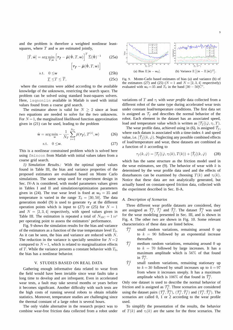
per operating point to assess the estimators’ performance.Fig. 9 shows the simulation results for the bias and variance

of the estimators as a function of the true temperature levelT0.As it can be seen, the bias and variance are reduced withN .The reduction in the variance is specially sensitive forN =2compared toN=1, which is related to marginalization effectsof T . While the variance presents a constant behavior withT0,the bias has a nonlinear behavior.

V. STUDIES BASED ON REAL DATA

Gathering enough informative data related to wear fromthe field would have been inviable since wear faults take along time to develop and are infrequent. Even in acceleratedwear tests, a fault may take several months or years beforeit becomes significant. Another difficulty with such tests arethe high costs of running several robots to obtain reliablestatistics. Moreover, temperature studies are challenging sincethe thermal constant of a large robot is several hours.

The only viable alternative in the research project was tocombine wear-free friction data collected from a robot under

30 32 34 36 38 40 42 44 46 48 50

−4

−2

0

2

4

T0 (C◦)

bia

s

N =1N =2N =3N =4

(a) BiasE [w − w0].

30 32 34 36 38 40 42 44 46 48 5010

15

20

25

30

35

40

45

50

T0 (C◦)

vari

ance

N =1N =2N =3N =4

(b) VarianceE[

(w − E [w])2]

.

Fig. 9. Monte-Carlo based estimates of bias (a) and variance (b) ofthe estimators (27) and (25) (N = 1 andN = [2, 3, 4] respectively)evaluated withw0=35 andT0 in the band[30− 50]C◦.

variations ofT andτl with wear profiledata collected from adifferent robot of the same type during accelerated wear testsunder constant load/temperature conditions. The first datasetis assigned asTf and describes the normal behavior of therobot. Each element in the dataset has an associated speed,load and temperature value which is written as[Tf ](ϕ, τl, T ).

The wear profile data, achieved using in (6), is assignedTf ,where each datum is associated with a time-indexk and speedvalue, i.e.[Tf ](k, ϕ). Neglecting any possible combined effectsof load/temperature and wear, these datasets are combined asa function ofk according to

τf (k, ϕ) = [Tf ](ϕ, τl(k), T (k)) + [Tf ](k, ϕ) (28)

which has the same structure as the friction model used inthe wear estimators, see (9). The behavior of wear withk isdetermined by the wear profile data used and the effects ofdisturbances can be examined by choosingT (k) and τl(k).Notice that these data are not analytically generated, butactually based on constant-speed friction data, collectedwiththe experiment described in Sec. II-A.

A. Description of Scenarios

Three different wear profile datasets are considered, theyare assigned asT 0

f , T 1f and T 2

f . The datasetT 0f was used

for the wear modeling presented in Sec. III, and is shown inFig. 4. The other two are shown in Fig. 10. Some relevantcharacteristics of these data are listed below.T 0f small random variations, remaining around 0 up

to k = 90 followed by an exponential increasethereafter.

T 1f medium random variations, remaining around 0 up

to k = 70 followed by large increases. It has amaximum amplitude which is56% of that foundin T 0

f .T 2f small random variations, remaining stationary up

to k=30 followed by small increases up tok=97from where it increases steeply. It has a maximumamplitude which is106% of that found inT 0

f .Only one dataset is used to describe the normal behavior offriction and is assigned asT 0

f . Three scenarios are consideredusing the dataset pairs(T 0

f , T0f ), (T

0f , T

1f ) and(T 0

f , T2f ). The

scenarios are called 0, 1 or 2 according to the wear profileused.

To simplify the presentation of the results, the behaviorof T (k) and τl(k) are the same for the three scenarios. The

10

TABLE IVCHOICE OF OPTIMAL SPEED VALUES FOR DIFFERENT VALUES OF

FRICTION OBSERVATIONSN .

Possible values:[2.1, 8.7, 15.3, 21.9, 28.5, 35.1, 41.7,82.2, 133.5, 184.7, 236.2, 287.1]

N Cost Φ∗

1 46.58 35.12 26.20 [35.1, 41.7]T

3 22.60 [28.5, 41.7, 82.2]T

4 18.00 [2.1, 28.5, 35.1, 41.7]T

associated behavior of wear-free friction for the scenarios andthe values ofT and τl are shown in Fig. 11. Notice that theamplitude of the friction changes due to temperature and loadare considerably larger than of those caused by wear for anyof the scenarios. The maximum change value found for thewear-free friction behavior is157% relative to the maximumchange found inT 0

f .The same parameters for the friction model and estimators

are used in all scenarios. The parameters for the estimatorsare given in (24). The model parameters used to describe thenormal behavior of friction, i.e. related toτf (ϕ, τl, T ) in (8),are given in Table I and were identified using the datasetT 0

f .The wear parameters used, i.e. related toτf (ϕ,w) in (8), aregiven in Table II and were identified using the datasetT 0

f .In this setting, the use of a dataset with superscript0

in a scenario, means that the related model parameters areconsidered correct otherwise they are uncertain. That is, thecorrect parameters forτf (ϕ, τl, T ) are considered availablein all scenarios while the wear parameters are uncertain forScenarios 1 and 2.

B. Results and Discussion

The datasets considered contain friction data collected un-der 12 different speed levels. The choice of speed valuesfor experiment design is thus limited to these speed levels.The problems (19) and (23) are solved by considering everypossible combination of speed level forN = [1, 2, 3, 4]. Theresulting optimal values are given in Table IV and relate wellto those found in Table III. Notice that the optimal valuesdepend on the wear model parameters used which in this caseis only consistent for Scenario 0.

The resulting wear estimates for the different scenarios areshown in Figs. 12(a) to 12(c). The same axes are used inthe figures so they are directly comparable. The shaded areahighlights a region which should be easily distinguishablefrom the rest in order to allow for a simple detection ofexcessive wear.

The wear estimates become smoother for largerN , whichis in line with the simulation study of Sec. IV-B. For allscenarios, the larger wear estimates fork > 90 allows fora distinction of the critical (shaded) regions. Noticeably, thewear estimates are consistent to the wear profile data used inall scenarios, even for Scenarios 1 and 2 when the wear modelis uncertain.

The fact that the wear estimates do not differ much withN

might lead to the conclusion thatN=1 should be used, but this

is only true if the optimal speed values are chosen. To illustratethis, wear estimates were achieved for Scenario 2 using onemeasurement forϕ=82.2 andϕ=133.5. As it can be noticed,the wear estimates are considerably affected by changes intemperature when these speed values are used. However,when these two measurements are used together, the estimatebecomes less sensitive. The inclusion of measurements aroundthe optimal speed values will also increase robustness touncertainties in the wear model. This is because the optimalspeed values depend on the wear model parameters used,which are typically unknown before a fault appears.

VI. CONCLUSIONS

From the simulation and experimental results, it is possibleto conclude that the simultaneous estimation of temperatureand wear, whenN ≥ 2, provides more reliable estimatescompared toN=1 when the marginalized likelihood functionin (27) is used. In general, it can be expected that additionalmeasurements will increase the estimates’ accuracy, with thetradeoff of an increased experiment time.

A natural extension to this work is to consider on-lineestimation, without the need for data collected from experi-ments. This could perhaps be achieved by considering datafrom a friction observer, e.g. as presented in [20], [21]. Thesensitivity of such approach to unmodeled phenomena, e.g.due to dynamic friction, and external disturbances should beconsidered carefully based on experiments performed on a realrobot in different applications.

The wear estimates could possibly be improved further incase estimates/measurements of the joint temperatures wereavailable. Joint temperature sensors are typically unavailablein applications, more common is perhaps the availability ofenvironment temperature sensors. In the later case, estimatesof the joint temperature are possible based on a known heattransfer model, e.g. using the approach presented in [8]. Thetemperature in the joints can also be possibly inferred basedon estimates of the motor temperature, which can be achievedbased on a known relation between temperature and the motorconstant, see e.g. [40].

The studies presented here are restricted to one type ofgearbox. It would be interesting to study the behavior offriction- and wear effects in other gear types. Also interestingis to consider other types of variations and how these affectthe models and framework presented. For example, a changeof lubricant may require the re-estimation of all or some ofthe friction parameters used.

For CBM, it is important to provide an accurate decisionon when to perform maintenance. Based on the laboratory teststudies presented, this should be done carefully. For example,while a threshold set at35 could be used for Scenarios 0and 1, the same threshold would give a too early detectionfor Scenario 2. A too early detection is understood as lesscritical than a total failure of the system but may lead tounnecessary maintenance actions. More careful analyses ofthe wear estimates may therefore be needed in order to givean accurate support for a maintenance decisions. Perhapsthe influence on the wear rate should also be considered in

11

050

100150

200250

300 0

20

40

60

80

100−0.01

0

0.01

0.02

0.03

0.04

0.05

kϕ (rad/s)

τf

τ0

f

(a) Wear profile dataT 1

f.

050

100150

200250

300 0

20

40

60

80

100−0.02

0

0.02

0.04

0.06

0.08

0.1

kϕ (rad/s)

τf τ0

f

(b) Wear profile dataT 2

f.

Fig. 10. Friction wear profile data used in Scenarios 1 (a) and 2 (b). The dashedline indicates a wear level to be found. The dotted linesrelate to the friction curveτ0

f before the wear tests started.

0

50

100

150

200

250

300 0

20

40

60

80

100

0

0.05

0.1

0.12

kϕ (rad/s)

τf offset: 0.0376

(a) Nominal friction behavior.

0 10 20 30 40 50 60 70 80 90 10030

35

40

45

50

k

T(C

◦)

0 10 20 30 40 50 60 70 80 90 1000

0.2

0.4

0.6

0.8

τl

τlT

(b) AssociatedT andτl.

Fig. 11. Behavior of normal (wear-free) friction as a function ofϕ andk for the scenarios considered (a); an offset value corresponding tothe smallest friction value in the dataset was removed for a comparison to the wear effects. The associated temperature and load values areshown in (b).

0 10 20 30 40 50 60 70 80 90 100

0

20

40

60

80

100

k

w

N =1N =2N =3N =4

(a) Scenario 0.

0 10 20 30 40 50 60 70 80 90 100

0

20

40

60

80

100

k

w

N =1N =2N =3N =4

(b) Scenario 1.

0 10 20 30 40 50 60 70 80 90 100

0

20

40

60

80

100

k

w

N =1N =2N =3N =4

(c) Scenario 2.

0 10 20 30 40 50 60 70 80 90 100

0

20

40

60

80

100

k

w

Φ=82.2Φ=133.5Φ=[82.2, 133.5]T

(d) Scenario 2 with non-optimal speed values.

Fig. 12. Wear estimates for the different scenarios investigated. Figs. (a) to (c)present the estimates forN =[1, 2, 3, 4] using the optimalspeed values. Fig. (d) illustrates Scenario 2 when non-optimal speed values are used forN =[1, 2]. The shaded area in the figures relatesto a region where a detection should be made.

12

the decision rule. The determination of the experimentationfrequency and remaining lifetime are also important. The studyof lifetime models is therefore important.

REFERENCES

[1] A. R. Lansdown, A. L. Price, and J. Larsen-Basse, “Materials to resistwear—a guide to their selection and use,”Journal of Tribology, vol.109, no. 2, pp. 379–380, 1987.

[2] J. A. Williams, “Wear and wear particles - some fundamentals,” Tribol-ogy International, vol. 38, no. 10, pp. 863 – 870, 2005.

[3] W. Seifert and V. Westcott, “A method for the study of wear particlesin lubricating oil,” Wear, vol. 21, no. 1, pp. 27 – 42, 1972.

[4] B. Roylance, “Ferrography - then and now,”Tribology International,vol. 38, no. 10, pp. 857 – 862, 2005.

[5] K. Kato, “Wear in relation to friction – a review,”Wear, vol. 241, no. 2,pp. 151 – 157, 2000.

[6] B. Freyermuth, “An approach to model based fault diagnosisof industrialrobots,” inProc. of the 1991 IEEE International Conference on Roboticsand Automation (ICRA), vol. 2, Sacramento, USA, Apr 1991, pp. 1350–1356.

[7] A. C. Bittencourt, “Friction change detection in industrial robot arms,”Master’s thesis, The Royal Institute of Technology, 2007, xR-EE-RT2007:026.

[8] L. Marton and F. van der Linden, “Temperature dependent frictionestimation: Application to lubricant health monitoring,”Mechatronics,vol. 22, no. 8, pp. 1078 – 1084, 2012.

[9] L. Marton, “On-line lubricant health monitoring in robotactuators,” inProc. of the 2011 Australian Control Conference (AUCC), Melbourne,Australia, nov. 2011, pp. 167 –172.

[10] V. Filaretov, M. Vukobratovic, and A. Zhirabok, “Observer-based faultdiagnosis in manipulation robots,”Mechatronics, vol. 9, no. 8, pp. 929– 939, 1999.

[11] M. McIntyre, W. Dixon, D. Dawson, and I. Walker, “Fault identificationfor robot manipulators,”IEEE Transactions on Robotics, vol. 21, no. 5,pp. 1028–1034, Oct. 2005.

[12] D. Brambilla, L. Capisani, A. Ferrara, and P. Pisu, “Fault detection forrobot manipulators via second-order sliding modes,”IEEE Transactionson Industrial Electronics, vol. 55, no. 11, pp. 3954–3963, Nov. 2008.

[13] A. De Luca and R. Mattone, “An adapt-and-detect actuator FDI schemefor robot manipulators,” inProc. of the 2004 IEEE InternationalConference on Robotics and Automation (ICRA), vol. 5, Barcelona,Spain, apr. 2004, pp. 4975 – 4980 Vol.5.

[14] S. C. Guo, M. H. Yang, Z. R. Xing, Y. Li, and J. Q. Qiu, “Actuatorfault detection and isolation for robot manipulators with the adaptiveobserver,”Advanced Materials Research, vol. 482 - 484, no. 8, pp. 529–532, 2012.

[15] F. Caccavale, P. Cilibrizzi, F. Pierri, and L. Villani,“Actuators fault diag-nosis for robot manipulators with uncertain model,”Control EngineeringPractice, vol. 17, no. 1, pp. 146 – 157, 2009.

[16] A. T. Vemuri and M. M. Polycarpou, “A methodology for faultdiagnosisin robotic systems using neural networks,”Robotica, vol. 22, no. 04, pp.419–438, 2004.

[17] A. De Luca and R. Mattone, “Actuator failure detection and isolationusing generalized momenta,” inProc. of the 2003 IEEE InternationalConference on Robotics and Automation (ICRA), vol. 1, Taipei, Taiwan,sept. 2003, pp. 634 – 639 vol.1.

[18] W. E. Dixon, I. D. Walker, D. M. Dawson, and J. P. Hartranft, “Fault de-tection for robot manipulators with parametric uncertainty:A prediction-error-based approach,”IEEE Tran. on Robotics and Automation, vol. 16,no. 6, pp. 3628–3634, 2000.

[19] A. De Luca and L. Ferrajoli, “A modified Newton-Euler method fordynamic computations in robot fault detection and control,” in Proc. ofthe 2009 IEEE International Conference on Robotics and Automation(ICRA), Kobe, Japan, may 2009, pp. 3359 –3364.

[20] L. R. Ray, J. R. Townsend, and A. Ramasubramanian, “Optimalfilteringand Bayesian detection for friction-based diagnostics in machines,”ISATransactions, vol. 40, no. 3, pp. 207 – 221, 2001.

[21] L. Le Tien, A. Albu-Schaffer, A. De Luca, and G. Hirzinger, “Frictionobserver and compensation for control of robots with joint torquemeasurement,” inProc. of the 2008 IEEE/RSJ International Conferenceon Intelligent Robots and Systems (IROS), Nice, France, sept. 2008, pp.3789 –3795.

[22] F. Abdollahi, H. Talebi, and R. Patel, “A stable neural network-basedobserver with application to flexible-joint manipulators,”IEEE Transac-tions on Neural Networks, vol. 17, no. 1, pp. 118 – 129, jan. 2006.

[23] T. Yuksel and A. Sezgin, “Model-based FDI schemes for robot manipu-lators using soft computing techniques,”InTech, 2010, ISBN: 978-953-307-037-7.

[24] Z. Bo, D. Bo, and L. Yuanchun, “Support vector machine observer basedfault detection for reconfigurable manipulators,” inProc. of the 30thChinese Control Conference (CCC), Changchun, China, july 2011, pp.3979 –3984.

[25] M. R. G. Meireles, P. E. M. Almeida, and M. G. Simoes, “A compre-hensive review for industrial applicability of artificial neural networks,”IEEE Transactions on Industrial Electronics, vol. 50, pp. 585–601, 2003.

[26] B. Halder and N. Sarkar, “Robust fault detection of a robotic manipu-lator,” Int. J. Rob. Res., vol. 26, no. 3, pp. 273–285, Mar. 2007.

[27] J.-F. Magni and P. Mouyon, “On residual generation by observer andparity space approaches,”IEEE Transactions on Automatic Control,vol. 39, no. 2, pp. 441 –447, feb 1994.

[28] V. Filaretov, M. Vukobratovic, and A. Zhirabok, “Parity relation ap-proach to fault diagnosis in manipulation robots,”Mechatronics, vol. 13,no. 2, pp. 141 – 152, 2002.

[29] W. Chen, “Fault detection and isolation in nonlinear systems: observerand energy-balance based approaches,” Dissertation, Faculty of Eng.Automatic Control and Complex Systems, Duisubug-Essen University,Oct 2011.

[30] L. Marton, “Energetic approach to deal with faults in robot actuators,”in Proc. of the 20th Mediterranean Conference on Control Automation(MED), Barcelona, Spain, july 2012, pp. 85 –90.

[31] I. Eski, S. Erkaya, S. Savas, and S. Yildirim, “Fault detection on robotmanipulators using artificial neural networks,”Robotics and Computer-Integrated Manufacturing, vol. 27, no. 1, pp. 115 – 123, Jul 2011.

[32] E. Olsson, P. Funk, and M. Bengtsson, “Fault diagnosis of industrialrobots using acoustic signals and case-based reasoning,” in Advances inCase-Based Reasoning, ser. Lecture Notes in Computer Science, P. Funkand P. A. Gonzalez Calero, Eds. Springer Berlin / Heidelberg, 2004,vol. 3155, pp. 13–15.

[33] A. C. Bittencourt and S. Gunnarsson, “Static friction in a robot joint—modeling and identification of load and temperature effects,”Journal ofDynamic Systems, Measurement, and Control, vol. 134, no. 5, 2012.

[34] A. C. Bittencourt, P. Axelsson, Y. Jung, and T. Brogardh, “Modeling andidentification of wear in a robot joint under temperature disturbances,”in Proc. of the 18th IFAC World Congress, Milan, Italy, Aug 2011.

[35] F. Al-Bender and J. Swevers, “Characterization of friction force dynam-ics,” IEEE Control Systems Magazine, vol. 28, no. 6, pp. 64–81, 2008.

[36] K. De Moerlooze, F. Al-Bender, and H. Van Brussel, “A generalisedasperity-based friction model,”Tribology Letters, vol. 40, pp. 113–130,2010.

[37] C. M. Bishop,Pattern Recognition and Machine Learning, 1st ed. NewYork, USA: Springer, 2007.

[38] H. L. Van Trees,Detection, Estimation and Modulation Theory, Part I.Wiley, New York, 2001.

[39] B. Porat and B. Friedlander, “Computation of the exact informationmatrix of Gaussian time series with stationary random components,”IEEE Transactions on Acoustics, Speech and Signal Processing, vol. 34,no. 1, pp. 118 – 130, feb 1986.

[40] X. Ding, J. Liu, and C. Mi, “Online temperature estimationof IPMSMpermanent magnets in hybrid electric vehicles,” inProc. of the 2011 6thIEEE Conference on Industrial Electronics and Applications (ICIEA),Beijing, China, june 2011, pp. 179 –183.

Andr e Carvalho Bittencourt graduated in Automatic Control Engineer withhonors from the Federal University of Santa Catarina, Florianopolis, Brazil.He received a Licentiate degree in January 2012 from Linkoping University,Sweden, where he is currently a Ph.D. student. His main research interestsare industrial robotics, diagnosis and condition monitoring.

Patrik Axelsson received the M.Sc. degree in applied physics and electricalengineering in January 2009 and the Licentiate degree in automatic controlin December 2011, both from Linkoping University, Sweden. His researchinterests are sensor fusion and control for industrial manipulators.

Avdelning, Institution

Division, Department

Division of Automatic ControlDepartment of Electrical Engineering

Datum

Date

2013-03-15

Språk

Language

� Svenska/Swedish

� Engelska/English

�

�

Rapporttyp

Report category

� Licentiatavhandling

� Examensarbete

� C-uppsats

� D-uppsats

� Övrig rapport

�

�

URL för elektronisk version

http://www.control.isy.liu.se

ISBN

�

ISRN

�

Serietitel och serienummer

Title of series, numberingISSN

1400-3902

LiTH-ISY-R-3058

Titel

TitleModeling and Experiment Design for Identi�cation of Wear in a Robot Joint under Load andTemperature Uncertainties based on Constant-speed Friction Data

Författare

AuthorAndré Carvalho Bittencourt, PAtrik Acelsson

Sammanfattning

Abstract

The e�ects of wear to friction are studied based on constant-speed friction data collectedfrom dedicated experiments during accelerated wear tests. It is shown how the e�ects oftemperature and load uncertainties produce larger changes to friction than those caused bywear, motivating the consideration of these e�ects. Based on empirical observations, an ex-tended friction model is proposed to describe the e�ects of speed, load, temperature andwear. Assuming availability of such model and constant-speed friction data, a maximumlikelihood wear estimator is proposed. A criterion for experiment design is proposed whichselects speed points to collect constant-speed friction data which improves the achievableperformance bound for any unbiased wear estimator. Practical issues related to experimentlength are also considered. The performance of the wear estimator under load and temper-ature uncertainties is found by means of simulations and veri�ed under three case studiesbased on real data.

Nyckelord

Keywords industrial robotics, wear, friction, identi�cation, condition monitoring