liquid carry-over in gas-liquid cylindrical cyclone...
TRANSCRIPT

i
T H E U N I V E R S I T Y O F T U L S A
THE GRADUATE SCHOOL
LIQUID CARRY-OVER IN GAS-LIQUID CYLINDRICAL CYCLONE (GLCC©)
COMPACT SEPARATORS FOR THREE-PHASE FLOW
by Srinivas Swaroop Kolla
A thesis submitted in partial fulfillment of
the requirements for the degree of Master of Science
in the Discipline of Mechanical Engineering
The Graduate School
The University of Tulsa
2007


iii
ABSTRACT
Srinivas Swaroop Kolla (Master of Science in Mechanical Engineering) Liquid Carry-Over in Gas-Liquid Cylindrical Cyclone (GLCC©) Compact Separators for Three-Phase Flow Directed by Dr. Ram S. Mohan
114 pp., Chapter 7
(195 words)
Prediction of the operational envelop for liquid carry-over is essential for proper
operation of Gas-Liquid Cylindrical Cyclone (GLCC) compact separators. The GLCC
operational envelop for liquid carry-over is studied experimentally and theoretically
under three-phase gas-oil-water flow.
Experimental data were acquired in a 3” diameter GLCC for the operational
envelop for liquid carry-over, under three-phase flow. Both light oil and heavy oil were
utilized, with watercuts ranging from 0 to 100 %. The liquid level was controlled at 6”
below the GLCC inlet.
A significant effect of watercut on the operational envelop for liquid carry-over
for three-phase flow has been observed. As the watercut reduces, the operational envelop
for liquid carry-over reduces, too. Also, the operational envelop for heavy oil reduces as
compared to light oil which could be primary due to the effect of viscosity. Finally, the
annular mist velocity increases with surface tension.

iv
A new model for the prediction of the operational envelop for liquid carry-over
for three-phase flow is presented. The proposed model incorporates the liquid level and
pressure control configuration, as well as the effect of watercut and fluid properties.
Good agreement is observed between the predicted results and the experimental data.
v
ACKNOWLEDGEMENTS
I would like to thank Dr. Ram S. Mohan and Dr. Ovadia Shoham for their
continuous patience and assistance on this project. Without their support and the
opportunity, I would not have been able to finish this work. I would also like to thank Dr.
Shoubo Wang and Dr. Luis Gomez for their support, guidance, and encouragement in
making this research possible and successful. I would like to thank Dr. Brenton S.
McLaury for his time serving on my thesis committee.
I wish to thank Dr. Vasudevan Sampath, Dr. Ciro Perez, and Dr. Nolides Guzman
who initially taught me how to work on the flow loop. I would like to extend my
gratitude and acknowledgement to Judy Teal for her personal support throughout this
work, as well as Mike Teal and Don Harris for expert technical assistance in installing
hardware for data acquisition and support in the Lab View software.
I wish to thank Tulsa University Separation Technology Projects (TUSTP) and
National Science Foundation Industry/University Cooperative Research Center on
Multiphase Transport Phenomena (NSF-I/UCRC -MTP) for providing me with the
financial support to conduct this research. I would like to thank TUSTP member
companies and graduate students for their valuable assistance during this project.
It is also important to acknowledge the Mechanical Engineering and Petroleum
Engineering Staff at The University of Tulsa for sharing their time and experience in
making this work meaningful and successful.

vi
I wish to acknowledge my friends for their continuous support and
encouragement all throughout my time and study here at the university. I thank my sister
Gowthami for supporting me and being there for me throughout my entire life. I thank
my cousin sister Haritha for being there whenever I needed someone here in the past
couple of years. Also, I would like to thank a special friend for the support I have
received during the past two years.
I dedicate this work to my parents, Kolla China Masthan Rao and Kolla
Visalakshmi, whose love and support were there throughout my life without which this
task would not have been accomplished.
vii
TABLE OF CONTENTS Page ABSTRACT .................................................................................................................... iii
ACKNOWLEDGEMENTS................................................................................................ v
TABLE OF CONTENTS.................................................................................................. vii
LIST OF TABLES............................................................................................................. ix
LIST OF FIGURES ........................................................................................................... xi
CHAPTER 1: INTRODUCTION ..................................................................................... 1
CHAPTER 2: LITERATURE REVIEW ......................................................................... 6 2.1 GLCC Experimental Studies and Field Applications.................................. 6 2.2 Hydrodynamic Flow Behavior Studies....................................................... 12 2.3 Mechanistic Modeling................................................................................... 14 2.4 Control System Studies................................................................................. 17
CHAPTER 3: EXPERIMENTAL PROGRAM ............................................................ 22
3.1 Experimental Facility ................................................................................... 22 3.1.1 Metering Section.............................................................................. 22 3.1.2 GLCC Test Section........................................................................... 25 3.1.3 Instrumentation and Data Acquisition System................................. 28
3.2 Physical Phenomena..................................................................................... 36 3.2.1 Liquid Carry-Over (LCO)................................................................ 37
3.3 Uncertainty Analysis..................................................................................... 40 3.3.1 Multiple-Measurement Uncertainty Analysis.................................. 40 3.3.2 Uncertainty Analysis Applied to Multiphase Metering.................... 44
CHAPTER 4: EXPERIMENTAL RESULTS AND DISCUSSION ............................ 48
4.1 Flow Pattern Map Experimental Data........................................................ 48 4.2 Operational Envelop..................................................................................... 49
4.2.1 Effect of Fluid Properties................................................................. 50 4.2.2 Effect of Watercut............................................................................ 51 4.2.3 Effect of Watercut on Annular Mist Velocity................................... 53
4.3 Uncertainty Analysis Results....................................................................... 54
viii
CHAPTER 5: MECHANISTIC MODELING .............................................................. 58 5.1 Inlet analysis.................................................................................................. 58
5.1.1 Inlet Flow Pattern Prediction.......................................................... 60 5.1.2 Nozzle Analysis for Stratified Flow.................................................. 61
5.2 Zero-Net Liquid Holdup .............................................................................. 65 5.3 Operational Envelop..................................................................................... 66
5.3.1 Flooding Point................................................................................. 68 5.3.2 Churn Region................................................................................... 69 5.3.3 Annular Mist Point........................................................................... 70
CHAPTER 6: COMPARISON OF MODEL PREDICTION WITH
EXPERIMENTAL DATA ...................................................................... 74 6.1 Prediction of Annular Mist Velocity ........................................................... 74 6.2 Prediction of Operational Envelop (OPEN)............................................... 74
CHAPTER 7: CONCLUSIONS AND RECOMMENDATIONS ................................ 77
7.1 Conclusions.................................................................................................... 77 7.2 Recommendations......................................................................................... 78
NOMENCLATURE ......................................................................................................... 79 REFERENCES ................................................................................................................. 83 APPENDIX 1: UNCERTAINTY ANALYSIS FOR LIGHT OIL DIFFERENT
WATERCUTS (LL=6” BELOW INLET) ............................................ 95 APPENDIX 2: UNCERTAINTY ANALYSIS FOR HEAVY OIL DIFFERENT
WATERCUTS(LL=6” BELOW INLET) ........................................... 105

ix
LIST OF TABLES Page 3.1: Liquid Level Set Point for Level Control .................................................................. 32
3.2: Properties of Gas Micro Motion® Coriolis Mass Flow Meter .................................. 34
3.3: Properties of Liquid Micro Motion® Coriolis Mass Flow Meter ............................. 35
3.4: Properties of Water Phase.......................................................................................... 36
3.5: Properties of Light Oil (Tulco Tech 80) .................................................................... 36
3.6: Properties of Heavy Oil (Lubsnap 1200)................................................................... 36
4.1: Fluid Properties of Different Fluids........................................................................... 50
4.2: Annular Mist Velocities at Different Watercuts........................................................ 52
4.3: Uncertainty Analysis of Light Oil with Different Watercuts .................................... 55
4.4: Uncertainty Analysis of Heavy Oil with Different Water Cuts................................. 56
A.1: Data Obtained From Light Oil Experiments (Part 1)................................................96
A.2: Data Obtained From Light Oil Experiments (Part 2)................................................97
A.3: Data Obtained From Light Oil Experiments (Part 3)................................................98
A.4: Standard Deviation of Data Obtained From Light Oil Experiments (Part 1) ........... 99
A.5: Standard Deviation of Data Obtained From Light Oil Experiments (Part 2) ......... 100
A.6: Standard Deviation of Data Obtained From Light Oil Experiments (Part 3) ......... 101
A.7: Uncertainty Pertaining to Individual Properties of Fluids (Light Oil Different Watercuts) ....................................................................................................................... 102 A.8: Uncertainty of Superficial Liquid Velocity (slv ) (Light Oil Different Watercuts) 103
A.9: Uncertainty of Superficial Gas Velocity (sgv ) (Light Oil Different Watercuts) .... 104

x
B.1: Data Obtained From Heavy Oil Experiments (Part 1) ............................................ 106
B.2: Data Obtained From Heavy Oil Experiments (Part 2) ............................................ 107
B.3: Data Obtained From Heavy Oil Experiments (Part 3) ............................................ 108
B.4: Standard Deviation of Data Obtained From Heavy Oil Experiments (Part 1)........ 109
B.5: Standard Deviation of Data Obtained From Heavy Oil Experiments (Part 2)........ 110
B.6: Standard Deviation of Data Obtained From Heavy Oil Experiments (Part 3)........ 111
B.7: Uncertainty Pertaining to Individual Properties of Fluids (Heavy Oil Different Watercuts) ....................................................................................................................... 112 B.8: Uncertainty Analysis of Superficial Liquid Velocity ( slv ) (Heavy Oil Different
Watercuts) ....................................................................................................................... 113 B.9: Uncertainty Analysis of Superficial Gas Velocity ( sgv ) (Heavy Oil Different
Watercuts) ....................................................................................................................... 114

xi
LIST OF FIGURES Page 1.1: S - Curve Showing the Growth of GLCC.................................................................... 2
1.2: Size Comparison of GLCC and Conventional Separators (Gomez, 1998).................. 3
1.3: Schematic of Single Inlet GLCC with Control Valves................................................ 4
3.1: Tanks, Pumps and Coriolis Micro MotionR Mass Flow Meter ................................. 23
3.2: NATCO Three Phase Separator................................................................................. 23
3.3: Schematic of Facility with the GLCC Test Section................................................... 24
3.4: Schematic of GLCC Test Section.............................................................................. 25
3.5: GLCC Inlet Section and Body................................................................................... 26
3.6: Front Panel of the VI used to Control the Experiment .............................................. 31
3.7: Front Panel of the VI Controlling Liquid Level........................................................ 31
3.8: Front Panel of the VI Used to Control the Pressure .................................................. 32
3.9: Operational Envelop for Light Oil with Different Watercuts.................................... 37
3.10: Schematic of Churn Flow in GLCC ........................................................................ 39
3.11: Schematic of Annular Flow in GLCC ..................................................................... 39
3.12: Uncertainity Analysis Procedure ............................................................................. 41
4.1: Experimental Data Flow Pattern Predictions at the Inlet Section of GLCC.............. 48
4.2: Operational Envelop for Liquid Carry-Over for Water ............................................. 49
4.3: Effects of Fluid Properties ......................................................................................... 51
4.4: Effect of Watercut on the Operation Envelop with Light Oil.................................... 52

xii
4.5: Effect of Watercut on the Operational Envelop with Heavy Oil ............................... 53
4.6: Effect of Watercut on the Annular Mist Velocity...................................................... 54
4.7: Uncertainty Analysis of Operational Envelop for Light Oil with Different Watercuts........................................................................................................................................... 57 4.8: Uncertainty Analysis of Operational Envelop for Heavy Oil with Different Watercuts........................................................................................................................................... 57 5.1: Schematic View of the Inclined Inlet of the GLCC................................................... 59
5.2: Stratified Flow Nomenclature and Geometry at the Inlet.......................................... 61
5.3: Velocity Components at the Inlet of the GLCC ........................................................ 65
5.4: GLCC Nomenclature for Mechanistic Model ........................................................... 67
5.5: Procedure to Determine the LCO Operational Envelop (Part 1) ............................... 72
5.6: Procedure to Determine the LCO Operational Envelop (Part 2) ............................... 73
6.1: Comparison of Annular Mist Velocities for Light Oil and Heavy Oil ...................... 75
6.2: Comparison of Experimental Data with Modeling Predictions for Light Oil ........... 75
6.3: Comparison of Experimental Data and Modeling Predictions for Heavy Oil ........... 76

1
CHAPTER 1
INTRODUCTION Nature by itself is the best separator, but mankind does not have the necessary
resources to extract the separated phases in their pure form. Therefore in the oil recovery
process, separation of different phases has always been the prime motive in the petroleum
industry for several decades. The advancement in the multiphase separation technology
has been hindered by increasing operational problems and economic pressures over
several years forcing the petroleum industry to seek less expensive and more efficient
alternative solutions to conventional gravity based separators. Conventional vessel-type
separators which are bulky, heavy and expensive have been relied in the past for several
decades by the petroleum industry. A new generation of compact separators called the
Gas Liquid Cylindrical Cyclone (GLCC©1) separators has become increasingly popular as
an attractive alternative to conventional separators. Significant advantages of the GLCC’s
are its compactness, lower weight, ease of operation, and lower cost when compared to
conventional separators.
Due to the wide variety of potential applications ranging from partial separation
to complete phase separation, GLCC is used as an alternative to vessel-type separators.
GLCC is not only used for bulk separation but also used for enhancing the performance
of multiphase meters, multiphase flow pumps and de-sanders through the control of gas-
liquid ratio. Other applications of the GLCC are as automated well testing units, gas
_________________________________________________
1 GLCC© - Gas Liquid Cylindrical Cyclone - copyright, The University of Tulsa, 1994.

2
knock out and pre-separation devices, flare gas scrubbers, slug catchers, downhole
separators, and primary separators (Shoham and Kouba, 1998, Gomez, 1998).
Figure 1.1 shows an S-type graph giving the current status of GLCC technology
with respect to other well known and well established technologies. More than 1300
GLCC units have already been installed and put to use in the field for various
applications in the USA and around the world.
Figure 1.1: S - Curve Showing the Growth of GLCC
Figure 1.2 shows the size comparison of GLCC versus a conventional type
separator. For an average flow rate of lq = 200,000 bbl/d and gq = 70 MMscf/d and
average operating pressure of 100 psig, the conventional separator would be
approximately the presented size and can be replaced by a GLCC, which is much smaller
in size, less than 1/5th and 1/50th of conventional vertical and horizontal separators
respectively, and easy to operate.
Emerging Growth Maturity
Vessel Type Slug Catcher
Conventional Horizontal and Vertical
Separators
Finger Storage Slug Catcher
GLCC’s
FWKO Cyclones
Hydrocyclones
Gas Cyclones

3
Figure 1.2: Size Comparison of GLCC and Conventional Separators (Gomez, 1998)
The GLCC separator is a vertically installed pipe mounted with a downward
inclined tangential inlet, with outlets for gas and liquid provided at the top and bottom
respectively. The two phases of the incoming mixture are separated due to the
centrifugal/ buoyancy forces caused by the swirling motion. The liquid is forced radially
towards the wall of the cylinder and is collected from the bottom, while the gas moves to
the center of the cyclone and is taken out from the top of the GLCC.
Performance of the GLCC is limited by two phenomena, namely the liquid carry-
over into the gas stream, termed as LCO (Liquid Carry-Over), and gas carry-under into
the liquid stream, termed as GCU (Gas Carry-Under). These phenomena are strongly
dependent on the flow patterns existing in the upper part, above the inlet for LCO and in
Horizontal Separator
(19ft x 75ft)
Vertical Separator (9ft x 35ft)
GLCC Compact Separator
(5ft x 20ft)

4
the lower part of the GLCC for GCU. It is necessary to predict these two phenomena for
optimum design and proper operation of the GLCC in the field.
Figure 1.3: Schematic of Single Inlet GLCC with Control Valves
The overall objective of the current study is to investigate experimentally and
theoretically the flow behavior in the upper part of the GLCC and mechanisms associated
with the LCO phenomena. The specific objectives of this study are given below.
1. Conduct experimental investigations to determine the operational envelop of
GLCC separator for liquid carry-over at different water-cuts for 3-phase (oil-
water-gas) flow.
2. Conduct experimental investigations to compare the effect of light oil and
heavy oil on the operational envelop of GLCC separator for 3-phase flow.

5
3. Modify the mechanistic model to predict the LCO operational envelop for 3-
phase flow in GLCC under liquid level and pressure control configuration.
4. Modify the GLCC performance code incorporating the above mechanistic
model.
A brief overview of the pertinent literature related to the field applications of
GLCC, mechanistic modeling, hydrodynamic flow studies and control studies is
presented in Chapter 2. Detailed experimental program which deals with the experimental
setup, data acquisition system and uncertainty analysis is discussed in Chapter 3.
Experimental studies conducted for Operational Envelop for liquid carry-over for three
phase (oil-water-gas) flow are presented in Chapter 4. Mechanistic model that is modified
for predicting the liquid carry-over for 3-phase flow in GLCC with control is elaborated
in Chapter 5. Comparisons of the mechanistic model predictions and the experimental
data are illustrated in Chapter 6. The conclusions and recommendations of the
investigation carried out in this study are enumerated in Chapter 7, followed by
Nomenclature, References and Appendices in which the detailed experimental data and
uncertainty analysis results are provided.

6
CHAPTER 2
LITERATURE REVIEW
The Gas-Liquid Cylindrical Cyclone (GLCC) Separator technology has been an
emerging technology in the petroleum industry. Its rise has been very promising to meet
the ever increasing demands of petroleum industry, thus providing an attractive
alternative to the conventional separator which has been in industry for more than 100
years. Compared to conventional separators, only few publications are available on the
optimal experimental design and performance modeling of the GLCC separator. Detailed
literature review on compact separators technology was given by Arpandi et al. (1995).
Shoham and Kouba (1998) presented the state-of-the art of GLCC technology. Mohan
and Shoham (1999) presented the design and development of GLCC for three-phase
flow. Extensive theoretical and experimental studies have been conducted to understand
the separation mechanisms for liquid carry-over and gas carry-under in GLCC. Below is
a brief overview and latest information of pertinent literature on some important aspects
of the compact separation technology studies.
2.1 GLCC Experimental Studies and Field Applications
There have been numerous studies carried out on GLCC with respect to design
and modeling for the separation process in GLCC and most of the studies are based on
experiments only. Davies (1984), Davies and Watson (1979) and Oranje (1990) studied
7
compact separators for offshore production with respect to weight, cost and separation
efficiency when compared to conventional separators. Oranje (1989) reported that full
scale performance of four types of gas-liquid separators indicated approximately 100%
efficiency for slug catching in such separators.
Bandyopadhyay et al. (1994), at the Naval Weapons Research Laboratory,
considered the use of cyclone type gas-liquid separators to separate hydrogen bubbles
from liquid sodium hydroxide electrolyte in aqueous aluminum silver oxide battery
systems. The cyclone used both a tangential inlet as well as a tangential outlet, with an
arrangement to change the relative angle between the two. It was found that the gas core
is sensitive to the relative angle between the inlet and outlet, and the aspect ratio of the
cylinder. Two basic core configurations were observed: straight and helical spiral. The
optimum angle for the most stable core was found to be a function of liquid flow rate and
separator geometry.
The cyclone separator used for gas-oil separation developed by Nebrensky et al.
(1980) included a tangential rectangular inlet, equipped with a special vane and shroud
arrangement to change the inlet area, which allowed control of the inlet velocity
independent of the throughput, and extended the operating range of the separator. This
cyclone also used a vortex finder for the gas exit.
A hollow gas-liquid separator with rectangular tangential inlet near the bottom of
the separator has been developed by Zhikarev et al. (1985). They determined the
geometrical dimensions and operating regimes at which the cyclone can operate with
minimum entrainment of liquid droplets based on their results of theoretical and
experimental investigations. A cylindrical cyclone with spiral vane internals called auger
8
separator was developed by ARCO (Kolpak, 1994) and exhibited 2% to 18% gas carry
under when tested in Alaska.
Weingarten et al. (1995) explored alternatives to conventional methods of
controlling liquid level inside separators by using throttling floats and throttling
diaphragm valves operated by the vessel hydrostatic head. These tests explored the
sensitivity of liquid level inside the cylindrical cyclone to the pressure drop in the liquid
and gas legs. Compact cyclone separators have also found applications in conjunction
with multiphase flow pumps. Arato and Barnes (1992) used an in-line free vortex
separator downstream of a centrifugal multiphase pump for gas-liquid separation. Part of
the separated liquid was then re-circulated into the pump to reduce the volumetric ratio of
the gas in the two-phase mixture at the pump inlet. This procedure improved the pump
capacity and performance.
Baker and Entress (1991) proposed a new design for a Vertical Annular
Separation Pumping System (VASPS) for sub sea separation and pumping facilities. This
system enables production from reservoirs in remote areas and marginal fields. They
found the wellhead separation and pumping to be an efficient method for large distance
transportation, particularly in deep water. Kanyua and Freeston (1985) experimentally
studied the possible application of a Vertical Flow Centrifugal Separator (VFCS) for
geothermal application. They reported the effect of geometry on separator efficiency for
downhole separation. The study was extended to surface operation following satisfactory
operation of downhole prototype. This separator design includes a vortex generator at the
inlet, a diffuser section and a gas vortex tube mounted in a compact configuration. It was
concluded that a vortex generator is desirable for above-surface, low pressure
9
applications while a larger diameter vortex tube is preferred for subsurface, high pressure
applications.
Davies and Watson (1979) developed miniaturized compact separators for
offshore platforms which require less space than conventional separators. These units
were found to be economically feasible and easy to operate. A cluster of vortex-tubes
have been developed by Porta-test Systems. The entire cluster is placed inside the vessel
type separator. Each vortex tube comprised of a central top opening for gas outflow,
peripheral bottom opening for liquid outflow and a side inlet tangential opening.
Forsyth (1984) used a similar design to separate liquid and dust particles from a
natural gas transmission system by placing a group of cyclone separators inside a
pressure vessel, producing dry clean gas eliminating the need to use oil bath or other filter
media.
One of the most enthusiastically explored applications of the GLCC is in
conjunction with multiphase metering systems. Below is the summary of the field
applications from a paper presented by Kouba et al. (2006). Chevron has successfully
built and operated several GLCC’s in low GOR flow metering applications. Liu and
Kouba (1994) and Kouba (1995) from Chevron conducted various studies for the
development of multiphase metering loop incorporating the Net Oil Computer, where gas
and liquid phases are separated by means of a GLCC separator and separately metered by
gas and liquid flow meters prior to recombination for transport.
A 6-inch diameter and 12-ft high single inlet GLCC at Texaco Humble test
facility was used (Kouba, 2002) to measure gas carry-under for various combinations of
10
crude oil, water and natural gas using nuclear densitometers located at the inlet vertical
riser and pipe section of the GLCC liquid exit.
Colorado Engineering Experimental Station Inc. (CEESI) tested (Wang et al.,
(2002a) a 6-inch dual inlet GLCC at pressures of 200 to 1000 psi, with natural gas and
decane. Both conventional and wet gas GLCC configurations were tested for gas and
liquid flow rates ranging from 25 MMscfd and 900 bbld respectively. When the GLCC
was equipped with annular film extractors (AFE) located above the GLCC lower and
upper inlets, the liquid carry-over significantly reduced beyond the normal operational
envelop.
Gas and liquid flow rates ranging from 34 Mscfd and 2000 bbld, respectively,
were used to test a 6-inch dual inlet GLCC multiphase metering system at Daqing oil
field experiment station with natural gas and crude oil for watercuts from 0 to 100 %
(Wang et al., 2006). A fully instrumented and integrated compact multiphase Inline
Water Separation (IWS) system which consists of Gas-Liquid Cylindrical Cyclone
(GLCC) separator, a Liquid-Liquid Pipe Separator (LLPS), a Liquid-Liquid Cylindrical
Cyclone (LLCC) separator and a two -stage Liquid-Liquid Hydrocyclone (LLHC) has
been tested at Daqing oil field experiment station to separate a significant portion of the
produced water from production stream, with the remaining production fluids (gas, oil
and reduced amount of water) sent to existing processing facilities.
A 60 in. ID and 20 ft tall GLCC, largest in the world was employed at Minas for
bulk separation/metering (Marrelli et al., 2000). This GLCC operated at 170 psia and
260oF, handling liquid and gas production rates of 160,000 bpd and 70 MMscfd,

11
respectively and is equipped with control valves on the gas and liquid legs and a
sophisticated control system for liquid level control.
GLCC’s were designed for Duri, Indonesia field to handle both sand production
and terrain slugging (Marrelli et al., 2000). Sensitivity Analysis of the conventional
separators vs. GLCC demonstrated that its application for Duri Area-10 alone was
estimated to improve the metering accuary considerable and save about $3.2 million over
conventional separators.
A 12-inch diameter and 12-ft high dual inlet wet gas configuration of the GLCC
was installed for metering application by CNOOC on an offshore platform in China
(Wang and Zhang, 2005). A dual inlet, 42-inch diameter 23-ft high GLCC was installed
by CNOOC for partial removal of gas (gas knockout) on an offshore platform which is
then flared.
The first GLCC for liquid knockout from a wet gas stream for raw gas lift
applications was installed in Nigeria (Bodunrin, et al., 1997) and demonstrated successful
scale-up of GLCC performance to high pressures. This GLCC was 12-inch diameter and
12-ft tall which separated 4 MMscfd of gas from about 500 blpd at 1700 psig.
GLCC’s with upstream slug damper inlet flow conditioning device (Kouba, 2002)
was installed in Duri, Indonesia. This slug damper has been further developed by TUSTP
and several units have been installed in California.
Chevron installed GLCC’s downstream of twin-screw multiphase pumps (Kouba,
1995) to separate and recirculate an adequate supply of liquid to the pump inlet,
protecting the pump from dryout since they are not designed to handle an inlet gas
content of higher than 95% GVF.
12
The first subsea GLCC application designed and constructed by Curtiss Wright
(Campen et al., 2006) has been developed by joint industry project led by Petrobras and
is located downstream of the multiphase pump, separating and recalculating liquid from
its liquid outlet back in to the pump suction.
2.2 Hydrodynamic Flow Behavior Studies
This section briefly describes the detailed studies carried out on the hydrodynamic
flow behavior in the GLCC. Millington and Thew (1987) reported local Laser Doppler
Anemometer (LDA) velocity measurements in cylindrical cyclone separators. Their
studies revealed that the distance between the inlet and outlet controlled the gas carry
under rate and they suggested the use of twin, diametrically opposite inlets for greater
axi-symmetry and gas core filament stability, leading to a much improved gas carry under
performance. They reported that cylindrical cyclone was superior to either the converging
or diverging cyclones in terms of best balance between carry under and carry over
performances and also they made an important observation which says that vortex
occurring in the cylindrical cyclone separator is a forced vortex with tangential velocity
structure.
Reydon and Gauvin (1981) studied the behavior of vortex flow in conical
cyclones. Their studies show that the magnitude of the inlet velocity does not change the
shape of the tangential velocity, axial velocity and the static pressure profiles. However,
the results showed that an increase in the inlet velocity increases the magnitude of all the
above quantities and the angle of the inlet does not have any effect on the static pressure
profile or the tangential pressure profile, but it has a small effect on the axial velocity
profile and it decreases the symmetry of the flow relative to the axis of the vortex. They
13
neglected the radial fluid velocity for design purposes as it was observed to be very small.
Static pitot tubes were used to measure the tangential velocities in a cylindrical cyclone
by Farchi (1990). His measurements confirmed that a forced vortex occurs in the
cyclone. However as the diameter of the cyclone increases, the velocity distribution tends
to match the free vortex profile.
Kurokawa and Ohtaik (1995) confirmed the existence of a complex velocity
profile by accurate single phase liquid flow measurements in a study on gas-liquid flow
characteristics in a spiral horizontal cyclone with a vortex generator. This study
distinguishes a forced vortex, generating a jet region with extremely high swirl velocity
around the pipe center, from a second swirl region formed by a free vortex near the wall
and also an intermediate region of backflow with high swirl velocity. This complex
velocity profile can be attributed to the gas inlet and outlet configurations.
Arpandi et al. (1996) carried out experiments to find out operational envelop
defining the conditions for which there will be no liquid carry-over or gas carry-under,
equilibrium liquid level, gas-liquid interface shape, velocity and holdup distributions and
pressure drop across the GLCC.
Movafaghian et al. (2000) acquired experimental data for three different inlet
geometries, four different liquid viscosities, three system pressures and effect of
surfactant. The experimental data comprises of equilibrium liquid level, zero-net liquid
flow holdup and operational envelop for liquid carry-over.
Erdal (2001) measured axial and tangential velocities and turbulent intensities
across the GLCC diameter at 24 different axial locations using a Laser Doppler
Velocitimeter (LDV). Measurements were conducted with water for liquid flow rates of

14
10, 30 and 72 gpm for different inlet configurations and outlet orientations for wide range
of Reynolds Numbers of about 5000 to 67,000. Measurements are used to create color
contour plots of axial velocity, tangential velocity and turbulent kinetic energy. Erdal
(2001) obtained large amounts of local measurements of swirling flow data for two-phase
swirling flow in the lower part of the GLCC and data on gas carry-under for air-water
flow.
Oropeza-Vazquez (2001) studied experimentally multiphase flow behavior in
Liquid-Liquid Cylindrical Cyclone (LLCC) and GLCC compact separators as free water
knockout devices. The single stage Gas-Liquid-Liquid Cylindrical Cyclone (GLLCC)
separation efficiency data reveal that it performs, in addition to the separation of the gas
phase, also as a free water knockout. This occurs only for low oil concentrations at the
inlet, below 10%.
Reinoso (2002) carried out experimental investigations on a flow conditioning
device namely, slug damper which can be used upstream of GLCC separator. He
measured propagation of liquid slug front in the damper, differential pressure across the
segmented orifice, GLCC liquid level, GLCC outlet liquid flow and static pressure in the
GLCC. His data proved that the slug damper is capable of dissipating long slugs,
ensuring fairly constant liquid flow rate in to the GLCC.
2.3 Mechanistic Modeling
There are very few mechanistic models that are published on topics related to
GLCC flow behavior. Wolbert et al. (1995) presented a mechanistic model for predicting
15
separation efficiency based on the analysis of droplet trajectories in liquid-liquid
hydrocyclones. A differential equation combining the models for the three bulk velocity
distributions namely, axial, radial, and tangential characterized the droplet trajectories. A
droplet diameter d100 was deduced corresponding to 100 % separation efficiency from the
critical trajectory characteristics.
Arpandi et al. (1996) developed a mechanistic model, capable of predicting the
general hydrodynamic flow behavior in a GLCC based on theoretical and experimental
studies conducted at Tulsa University Separation Technology Projects (TUSTP). The
model predicts simple velocity distributions, gas-liquid interface shape, equilibrium
liquid level, total pressure drop and operational envelop.
Marti et al. (1996) presented the analysis of bubble trajectory for GLCC
separators and the model predicts the gas liquid interface (vortex) near the inlet as a
function of the radial distribution of the tangential velocity. The bottom of the vortex
defines the starting location for the bubble trajectory analysis, which enables the
determination of separation efficiency based on the gas bubble size.
Experimental data on the hydrodynamic flow behavior study on the effects of
geometry, fluid physical properties and pressure were presented by Movafaghian et al.
(2000). This data was utilized to check and refine the GLCC mechanistic model
developed previously by Arpandi et al. (1996) and the comparisons showed good
agreement between the experimental data and the modified model.
Steady state and dynamic models were developed as framework for the GLCC
passive and active control system by Wang (1997). This steady state model was used to
analyze the system sensitivity, and the dynamic model was used to analyze the system

16
stability by applying linear control theory. A preliminary control strategy was proposed
for GLCC active control based on separated outlet configuration for gas and liquid
streams.
Gomez (1998), based on an improved mechanistic model, built a design code and
performance code which enable detailed prediction of the complex multiphase flow
behavior in the GLCC. An enhancement is incorporated in the flow pattern dependent
nozzle analysis for GLCC inlet for the prediction of the gas and liquid tangential
velocities at the GLCC entrance by Gomez et al. (1998).Gomez et al. (1999) developed A
state-of-the Art Simulator for field applications of GLCC separators.
An improved bubble trajectory model was presented utilizing the set of
correlations developed by Mantilla et al. (1999) based on the predictions of velocity field
(tangential and axial) in the GLCC separator.
A new mechanistic model to predict the aspect ratio of the GLCC, incorporating
an analytical solution for the gas-liquid interface shape, and a unified particle trajectory
model for bubbles and droplets was proposed by Gomez et al. (1999).
A mechanistic model was developed by Chirinos et al. (2000) to predict the
percent liquid carry over using the liquid carry over data acquired and the model was also
extended for high pressure conditions. The mechanistic model showed good agreement
with predictions for churn flow conditions and experimental data.
Gomez (2001) developed a mechanistic model for the characterization of this
complex flow behavior for predicting the gas carry-under in the GLCC. The above model
included gas entrainment in the inlet region, continuous phase-swirling flow behavior in
the lower part of the GLCC, dispersed phase particle motion, diffusion of dispersed

17
phase, coupled Eulerian-Lagrangian analysis, Lagrangian-Bubble Tracking Analysis and
simplified Mechanistic models.
Oropeza-Vazquez et al. (2004) developed mechanistic model for the prediction of
complex flow behavior and the separation efficiency in the LLCC and GLLCC which
include inlet analysis, droplet size distribution, and separation model based on droplet
trajectories in swirling flow.
A mechanistic model was developed by Reinoso (2002) for prediction of
hydrodynamic flow behavior in the slug damper. This model enables the prediction of the
outlet liquid flow rate and the available damping time, and in turn the prediction of the
slug damper capacity.
Pereyra (2005) developed a dynamic model and simulator for the Gas-Liquid
Cylindrical Cyclone/Slug Damper (GLCC-SD) system, for the prediction of its flow
behavior under transient slugging flow conditions. The GLCC-SD simulation results
demonstrate clearly the advantage of this system in dampen and smoothen the liquid flow
rate under slugging flow conditions, providing approximately constant flow rate at the
GLCC outlet liquid leg.
2.4 Control System Studies Various studies and experimental investigations have made the investigators
realize that the performance of the GLCC separators can be enhanced by incorporating
suitable control systems. A hydrostatic model for passive control system for liquid level
control inside a compact gas-liquid separator was developed by Kolpak (1994) where a
change in the liquid level is the driving signal for the liquid control valve and/or gas

18
valve. It was not applicable for slug flow or large or sudden variations in the fluid flow
rates although it was able to handle slow and steady variations in liquid level. The liquid
level was less sensitive to the inflow rates if the pressure drop across the compact
separator is relatively small and for the same pressure the liquid level was more sensitive
to the liquid flow rate rather than the gas flow rate. Hence the author suggested that if the
inflow rates change very slowly, a passive control system can be used effectively to
achieve liquid level control.
Gas-liquid two-phase separators usually operate under slug flow conditions in
actual field conditions, as the inflow rates seldom change slowly. Therefore system
dynamics are very crucial for such operations especially when a control system is added
to the separator. Genceli et al. (1988) developed a dynamic model for liquid level control
and pressure control configurations for slug catcher and PI controllers for both the control
loops. A slug catcher is a big vessel used as a preliminary separator upstream of a
conventional gas-liquid separator. Because of the large residence time of the big vessel,
the system response of the slug catcher was found to be quite slow.
A control algorithm in digital controllers was developed by Roy and Smith (1995)
to meet the goal of averaging level control for a single-phase surge tank system in
chemical processes. Galichet et al. (1994) presented the development of fuzzy logic
controller that maintains a floating level in a tank (single-phase flow) on top of an
atmospheric distillation unit of a refinery.
Following is a brief outline of the adaptive control strategies and its potential in
improving the existing compact separator control. An innovative method of self tuning
the controller to adapt to drastic changes in the process variable is known as Adaptive
19
control strategy. Ziegler-Nichols (1942) tuning rules were the very first documented
tuning rules developed for PID controller. Gorez (1997) developed different tuning rules
based on the same tuning procedures.
Vrancie et al. (1996) developed an indirect tuning method based on implicit
process model by using Magnitude Optimum Multiple Integration (MOMI) method. Luo
et al. (1998) proposed a simple method for auto-tuning a PID controller, which keeps the
controller in a closed loop. A new and innovative method of tuning PID controllers called
Pattern Recognition Approach was proposed by Kraus and Myron (1984).
A dynamic model for control of GLCC liquid level and pressure, using classical
control techniques was developed by Wang (1997). These investigations on GLCC
control showed that liquid level control can be achieved very effectively by using a
control valve in the liquid outlet for gas dominated systems and by using a control valve
in the gas outlet for liquid dominated systems. This innovative control system approach
formed the basis for GLCC active control system optimization.
Wang et al. (1998) and Mohan et al. (1998) carried out an extensive study on
passive control system, which utilized only the liquid flow energy. Detailed experimental
and modeling studies have been conducted to evaluate the improvement in the GLCC
operational envelope for liquid carry-over with passive control system. The results
showed that a passive control system is feasible for operation during normal slug flow
conditions.
Wang (2000) developed a control system dynamic simulator for GLCC
separators, based on Matlab/simulink software, for evaluation of several different GLCC
control philosophies for two-phase flow metering loop and bulk separation applications.

20
Wang et al. (2000) also developed an integrated level and pressure control system for
GLCC. Simulation studies for integrated control system demonstrated that the integrated
level and pressure control system is highly desirable for slugging conditions. Most of the
control strategies discussed above are based on feedback control.
A predictive (feed forward) control strategy was developed by Earni et al. (2001)
that can detect incoming slugs and enable control system to take preventive action in
controlling liquid level inside the compact separator. A new strategy for predictive
control, which integrates the feedback and feed forward loops, was proposed to
compensate for error due to modeling and slug characterization. Experimental results
demonstrated that the predictive control strategy was a viable approach for GLCC
separator control.
Wang et al. (2000a) developed a very unique, innovative technique, yet simple
control strategy called optimal control strategy which is capable of optimizing the
operating pressure and adapting to liquid and gas inflow fluctuations for GLCC
separators. Detailed experimental investigations and simulations conducted to evaluate
the performance of this optimal control system made compact separators robust and
increased the potential for offshore and sub-sea applications.
Avila (2003) carried out experiments on an integrated compact separation system
consisting of GLCC and LLCC in series using a gas control valve for controlling the
GLCC liquid level and liquid control valve for controlling the LLCC underflow watercut
to investigate its performance as three-phase oil-water-gas separator. The GLCC/LLCC
system simulator, developed by combining the linear models of GLCC and LLCC

21
control, was successfully tested for different perturbations, such as changes of set points
and flow rates, and different applications such as start-up and shut-down operations.
Sampath et al. (2004) at the Tulsa University Separation Technology Projects
(TUSTP) developed an adaptive control strategy for GLCC separator. Detailed
experimental investigations demonstrate that the proposed new optimal control system
with an inbuilt adaptive tuning algorithm is capable of controlling the liquid level and
reducing the dynamics of the liquid control valve. Recently, Sampath (2006) developed
control strategies for compact multiphase separation system (CMSS©). A similar CMSS
system was developed by Wang et al. (2006) for in-line water separation (IWS)
application.
A considerable progress has been achieved in the research conducted at Tulsa
University Separation Technology Projects (TUSTP), especially in the area of multiphase
flow systems. The two limiting phenomena, namely liquid carry-over and gas carry-
under, which control the operation of GLCC have been dealt in specific detail for
understanding the underlying principles.
The overall objective of the present study is to enhance the GLCC technology
focusing on the performance analysis of the operational envelop for liquid carry-over in
GLCC separator. The present study also includes new experimental results focusing the
effects of fluid properties, and water-cut on the operational envelop. The results are used
to modify the TUSTP mechanistic model to predict the operational envelop and develop a
design code with the proposed mechanistic model.
22
CHAPTER 3
EXPERIMENTAL PROGRAM
This chapter provides a detailed explanation of the experimental facility, physical
phenomena that occur in GLCC and uncertainty analysis pertaining to the experiments.
3.1 Experimental Facility Experimental data were acquired using advanced state-of-the-art instrumentation
and data acquisition system in a three-phase experimental flow loop which comprises of a
metering section to measure the single phase gas and liquid flow rates and a GLCC test
section.
3.1.1 Metering Section The metering section consists of three parallel, single phase feeder lines for
measuring the incoming single-phase gas and liquid flow rates. Three phase mixture is
formed at the mixing tee and delivered to the GLCC test section.
Air is used as the gas phase, which is supplied to a gas tank by an air compressor
with a capacity of 250 cfm at 108 psia. The gas flow rate into the loop is controlled by a
control valve and metered utilizing Micro Motion® mass flow meter.
The liquid phases are mineral oil of specific gravity 0.854 and water. The two
liquid phases are supplied from 400 gallon storage tanks at atmospheric pressure, and
pumped to the liquid feeder lines with centrifugal pumps as shown in Figure 3.1. Similar

23
to the gas phase, the liquid rate is controlled by separate control valves and metered using
the respective Micro MotionR mass flow meters.
Figure 3.1: Tanks, Pumps and Coriolis Micro MotionR Mass Flow Meter
Figure 3.2: NATCO Three Phase Separator

24
The single phase gas and liquid streams are combined at the mixing tee. Check
valves located downstream of each feeder are provided in order to prevent probable
backflow. The three phase mixture downstream of the test section is separated utilizing a
conventional three-phase separator as shown in Figure 3.2. Gas is vented into the
atmosphere and liquid is returned to the storage tank to complete the cycle. The
schematic of the flow loop is given in Figure 3.3.
Figure 3.3: Schematic of Facility with the GLCC Test Section
25
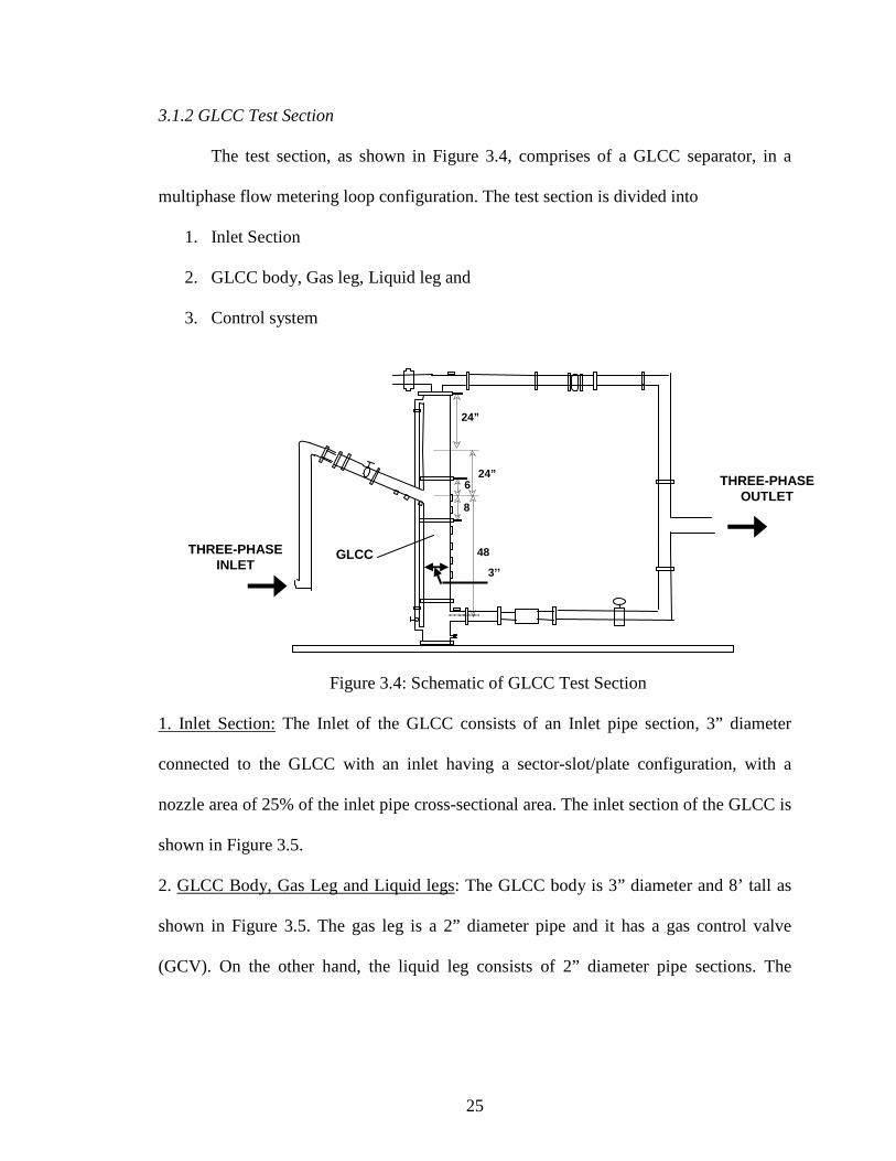
3.1.2 GLCC Test Section The test section, as shown in Figure 3.4, comprises of a GLCC separator, in a
multiphase flow metering loop configuration. The test section is divided into
1. Inlet Section
2. GLCC body, Gas leg, Liquid leg and
3. Control system
Figure 3.4: Schematic of GLCC Test Section
1. Inlet Section: The Inlet of the GLCC consists of an Inlet pipe section, 3” diameter
connected to the GLCC with an inlet having a sector-slot/plate configuration, with a
nozzle area of 25% of the inlet pipe cross-sectional area. The inlet section of the GLCC is
shown in Figure 3.5.
2. GLCC Body, Gas Leg and Liquid legs: The GLCC body is 3” diameter and 8’ tall as
shown in Figure 3.5. The gas leg is a 2” diameter pipe and it has a gas control valve
(GCV). On the other hand, the liquid leg consists of 2” diameter pipe sections. The
8
24”
48
624”
THREE-PHASE INLET
THREE-PHASE OUTLET
GLCC 3’’

26
Coriolis Micro Motion® mass flow meters are located on both gas leg and liquid leg to
measure the gas and liquid outflow rates respectively.
Figure 3.5: GLCC Inlet Section and Body
3. Control System: The main objective of the control system is to maintain the liquid
level in the GLCC by using the Control Valve. There are two simple control strategies
and two integrated control strategies mentioned below. Each of the control strategies
explained below has one final aim i.e. to control the liquid level in the GLCC. An
integrated liquid level and pressure control by LCV and GCV i.e. the third kind is used to
conduct experiments.
a) Liquid level control using liquid control valve (LCV)
b) Liquid level control using gas control valve (GCV)
c) Integrated liquid level and pressure control by LCV and GCV

27
d) Integrated liquid level control using both LCV and GCV
a) Liquid Level Control Using Liquid Control Valve (LCV)
This is a simple PID control loop where the process variable is the liquid level
signal from the differential pressure transducer. The set point liquid level is a manual
input to the controller. The output of the controller is a 4-20 mA signal that is fed to the
liquid control valve on the liquid leg of the GLCC separator.
b) Liquid Level Control Using Gas Control Valve (GCV)
The process variable in this strategy is the liquid level inside the GLCC separator
measured by a differential transducer. Liquid level is maintained at the desired set point
by the controller whose output is connected to the GCV. Operation of the GCV creates a
back-pressure, which in turn controls the liquid level inside the separator.
c) Integrated Liquid level and Pressure Control by LCV and GCV
This control strategy consists of two controllers. Liquid level is controlled by
controller acting on LCV and pressure inside GLCC is controlled by the second
controller operating the GCV. For the controller acting on LCV, the process variable is
the liquid level whereas for the controller acting on GCV the process variable is the
pressure in the GLCC.
d) Integrated Liquid Level Control Using Both LCV and GCV
Single process variable, which is the liquid level, is controlled by two independent
controllers. One controller acts on the GCV and the other acts on the LCV. The main
objective of this control system is to control the liquid level inside the GLCC operating
LCV and GCV simultaneously.
28
3.1.3 Instrumentation and Data Acquisition System
The GLCC is equipped with a level indicator (sight gauge) installed parallel to the
body of the separator. It is a transparent pipe that is connected to the bottom and top of
the GLCC body to give a visual idea of the level in the separator. It is also equipped with
a differential pressure transducer, which gives a measure of the liquid level. The
separated gas and liquid phases are metered by means of Micro Motion® mass flow meter
located downstream of the GLCC test section along with the temperature and density of
the liquids and gas. The absolute pressure transducers located at the inlet and top of the
GLCC measure the absolute pressure at respective locations.
The output signals from the sensors, transducers and metering devices are
connected to a central panel, which is connected to the computer through an A/D
converter. A data acquisition system is setup in the computer to acquire data from the
instruments. Data acquisition system used consists of different components namely;
sensors, transducers, control valves and flow meters, which send a 4-20mA signal
representing the physical quantity that it measures or controls. These signals are
connected to respective input/output boards of the National Instruments hardware for data
acquisition. National Instruments data acquisition system consists of the input/output
boards, SCXI 1101 Multiplexing Module, which is wired to the PCMCIA data collection
board fixed in the computer and the LabView software which could be programmed to do
multiple tasks like data collection, control process variable, etc. Sampling frequency of 2
Hz was used for light oil and 5 Hz was used for heavy oil. A total of 1500 data points
were averaged for each operating condition. A “virtual instrument” (VI) interface is
developed, using the LabView software application program which integrates

29
measurement, data acquisition, and interactive data processing for feedback control and is
capable of displaying signal online either digitally or graphically and can be downloaded
by saving it as a file or a spreadsheet to be analyzed at a later stage. A regular calibration
procedure employing a high-precision pressure pump is performed on each pressure
transducer at a regular schedule to guarantee the precision of measurements. The
temperature transducer consists of a Resistive Temperature Detector (RTD) sensor and an
electronic transmitter module.
LabView Software: LabView is a National Instruments software tool for
designing tests, measurements, and control systems. Using this integrated LabView
environment to interface with real-world signals and analyze data for meaningful
information, it is possible to create applications ranging from monitoring to sophisticated
simulation and control systems.
Applications of Labview:
1. Acquire data from a data acquisition device
2. Communicate with and control an instrument
3. Acquire data from a sensor
4. Process and analyze measurement data
5. Design a Graphical User Interface (GUI)
6. Save measurement data to file
A virtual interface, VI, of Labview is a user interface developed by using a set of
tools and objects known as front panel and coded using graphical representations of

30
functions to control the front panel objects known as block diagram. It can be said that
block diagram represents a flow chart in some ways.
The front panel is the user interface of the VI built with control and indicators which
are interactive input and output terminals of the VI, respectively. Controls are knobs,
push buttons and dials whereas indicators are graphs, LED’s and other displays. A block
diagram is built only once the front panel is built. The block diagram contains of the
source code to run the whole program and the front panel objects appear as icons or data
type terminals on the block diagram.
Front Panel of the LabView Program: The front panel of the labview program
used to carry out experiments is shown in Figure 3.6 which has different sections. They
can be classified as input section where the gas and liquid input flow rates into the GLCC
are monitored and controlled using this panel. It also contains the displays to monitor the
output of the GLCC which can give an idea of Gas Carry-Under (GCU) or Liquid Carry-
Over (LCO). This front panel also contains displays to monitor the pressure and
temperature in various sections of the flow loop. As can be seen in Figure 3.6 it has a
green push button and a blue push button denoted by “Press to Pressure in GLCC” and
“Press to adjust Level control” respectively. These are different sub VI’s (Virtual
Instruments) used to control the pressure and level in the GLCC as given by their names.
As shown in Figure 3.6 the top section is used to control the input of the liquid
and gas flow rates namely; water, oil and air. The output liquid and gas flow rates are
read through the Coriolis Micro Motion® mass flow meters and are displayed in the VI.
The sub VI’s for level control and pressure control are shown in Figures 3.7 and 3.8,
respectively.

31
Figure 3.6: Front Panel of the VI used to Control the Experiment
Figure 3.7: Front Panel of the VI Controlling Liquid Level
32
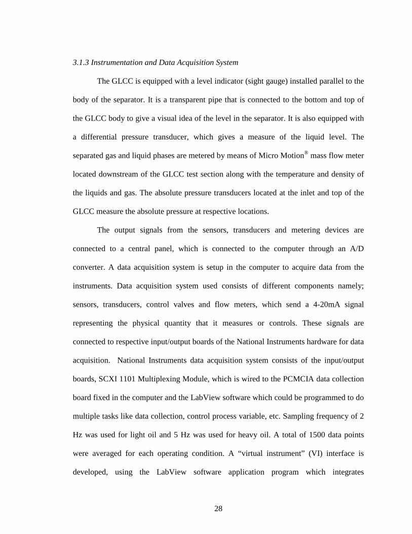
The sub VI to control the liquid level is shown in Figure 3.7 and it contains a set
point level and a measured level. The set point for the liquid level is modified based on
the watercut of the incoming liquid stream as shown in Table A graphical plot which
plots the set point level and measured level as a function of time is also shown. This can
be worked in 2 different modes i.e. Auto/Manual highlighted by green button. Similarly,
a sub VI has been written to control the pressure in the GLCC at a set point pressure as
shown in Figure 3.8.
Table 3.1: Liquid Level Set Point for Level Control
Watercut 0 25 50 75 100 Light Oil-Inches of
water 35.86 37.4 38.93 40.46 42 Heavy Oil-Inches of
Water 38.64 39.48 40.32 41.16 42
Figure 3.8: Front Panel of the VI Used to Control the Pressure

33
Flow Metering: Several watercut meters have been introduced to the oil industry
in the last few years for measuring oil and water concentrations. Particular concern is the
ability of a meter to provide accurate information for a wide range of flow conditions,
such as in the presence of gas. These meters use different techniques in order to measure
the water concentration in an oil-water mixture. Coriolis Micro Motion® mass flow meter
has been used in this study to measure the densities and mass flow rate through the
system.
Coriolis Mass Flow Meter (Micro Motion®): A Coriolis device such as Micro
Motion® mass flow-meter measures the mass flow rate and mixture density. Thus it
simultaneously serves as both a flow meter and watercut analyzer. Knowing the pure
phase densities, the mixture density of the mass flow meters can be used to calculate the
watercut dynamically assuming that there is no gas in the liquid stream. The major
components of the meter are a sensor and a transmitter.
The orientation of a Micro Motion® mass flow meter is normally recommended
by the manufacturer, and it is based on the particular metering application. For liquid
metering, a tubes-down installation is recommended to allow any entrained gas to be
easily moved out of the tube by buoyancy forces, even at low liquid flow rates. For gas
metering, a vertical tubes-up installation is recommended.

34
Benefits of Coriolis Mass Flow Meters (Micro Motion®): Superior accuracy and
repeatability ensure reliable performance regardless of conditions.
a) Easy to incorporate in to the process as there is no need for special mounting
techniques.
b) No erosion or corrosion as it doesn’t have any moving parts and hence reliable
in data.
c) Ability to handle transient two phase flow and minimal pressure drop within
the meter.
Gas flow rate was measured with a Coriolis Micro Motion® mass flow meter
model CMF100M32NUR. Liquid flow rate was measured with a Coriolis Micro Motion®
mass flow meter model CMF050M313NUR. The details of the various parameters are
given in Tables 3.2 and 3.3.
Table 3.2: Properties of Gas Micro Motion® Coriolis Mass Flow Meter
Nominal Pipe Diameter 25.4 mm
Nominal Flow Rate Range 0 to 3865 m3/h
Maximum Flow Rate 7100 m3/hr
Mass Flow Repeatability + 0.25 % of rate
Resolution 0.1 lbm/min
Zero Stability 0.526 m3/hr
Accuracy of Mass Flow Rate + 0.5 % of rate

35
Table 3.3: Properties of Liquid Micro Motion® Coriolis Mass Flow Meter
Nominal Pipe Diameter 12.7 mm
Nominal Flow Rate Range 0- 3.4 m3/hr
Maximum Flow Rate 6.8 m3/hr
Mass Flow Repeatability + 0.05 % of rate
Resolution 0.1 lbm/min
Zero Stability 1.63 *10-4 m3/hr
Accuracy Mass Flow Rate + 0.10 % of rate
Working Fluids: The working fluids used in this study are tap water and mineral oils
(Tulco Tech 80 & Lubsoil Lubsnap 1200). A red colored dye was added to the Tulco
Tech 80 mineral oil in order to improve flow visualization between the phases. It is
marketed by a local company (Tulco Oils Inc.). Typical properties of the different phases
are shown in Tables 3.4, 3.4, 3.5.
The criteria for selecting the oil are as follows:
• Low emulsification
• Fast separation
• Appropriate optical characteristics
• Non-degrading properties
• Non-hazardous

36
Table 3.4: Properties of Water Phase
Density, @ 70oF 1.0 ± 0.0003 g/cm3
Viscosity, @ 70oF 1.25 ± 0.15 cP
Table 3.5: Properties of Light Oil (Tulco Tech 80)
Gravity, API 33.2 Pour Point, oF +10
Viscosity SUS @ 100 F 85 Flash Point, oF 365 Color, saybolt +20
Table 3.6:- Properties of Heavy Oil (Lubsnap 1200)
Gravity, API 19.5 Pour Point, oF +15
Viscosity SUS @ 100 F Viscosity SUS @ 210 F
1250 69
Flash Point, oF 430 Color, ASTM L 1.0
3.2 Physical Phenomena
The Performance of GLCC is limited by two undesirable physical phenomena
namely Liquid Carry-Over (LCO) in the gas outlet stream and Gas Carry-Under (GCU)
in the liquid outlet stream. The ability to predict these two phenomena will ensure
optimum design parameters for the operation of the GLCC.
37
3.2.1 Liquid Carry-Over (LCO) Initiation of liquid entrainment into the discharged gas stream at the top of GLCC
is called as Liquid Carry-Over (LCO). LCO plays an important role in the analysis of the
performance of the GLCC. Earlier studies on the LCO were conducted mainly with two-
phase flow of water as the liquid medium and air as the gas medium. The current study is
concentrated on capturing the effect of oil properties and the effect of watercut on the
liquid carry over operational envelop of a GLCC in which the liquid level and pressure
are controlled.
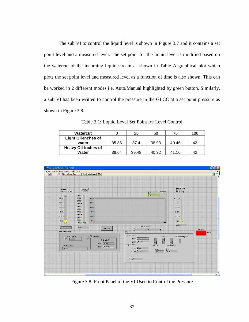
Operational Envelope: This section gives a detailed view of the operational
envelope with level control and pressure control in the GLCC. The operational envelop
for liquid carry-over is defined as the loci of vsl and vsg for which the liquid starts to get
carried into the gas leg. It occurs under extreme operating conditions of high gas and/or
high liquid flow rates. Plotting the loci of the liquid and gas flow rates at which LCO is
initiated provides the operational envelop for liquid carry over as illustrated in the Figure
3.9.
Figure 3.9: Operational Envelop for Light Oil with Different Watercuts
LCO REGION (a) (b) (c)
vsg
vsl
38
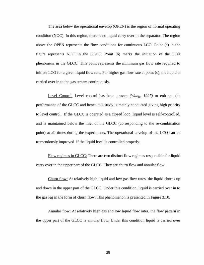
The area below the operational envelop (OPEN) is the region of normal operating
condition (NOC). In this region, there is no liquid carry over in the separator. The region
above the OPEN represents the flow conditions for continuous LCO. Point (a) in the
figure represents NOC in the GLCC. Point (b) marks the initiation of the LCO
phenomena in the GLCC. This point represents the minimum gas flow rate required to
initiate LCO for a given liquid flow rate. For higher gas flow rate at point (c), the liquid is
carried over in to the gas stream continuously.
Level Control: Level control has been proven (Wang, 1997) to enhance the
performance of the GLCC and hence this study is mainly conducted giving high priority
to level control. If the GLCC is operated as a closed loop, liquid level is self-controlled,
and is maintained below the inlet of the GLCC (corresponding to the re-combination
point) at all times during the experiments. The operational envelop of the LCO can be
tremendously improved if the liquid level is controlled properly.
Flow regimes in GLCC: There are two distinct flow regimes responsible for liquid
carry over in the upper part of the GLCC. They are churn flow and annular flow.
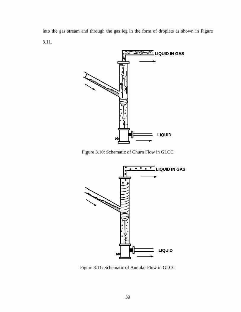
Churn flow: At relatively high liquid and low gas flow rates, the liquid churns up
and down in the upper part of the GLCC. Under this condition, liquid is carried over in to
the gas leg in the form of churn flow. This phenomenon is presented in Figure 3.10.
Annular flow: At relatively high gas and low liquid flow rates, the flow pattern in
the upper part of the GLCC is annular flow. Under this condition liquid is carried over
39
into the gas stream and through the gas leg in the form of droplets as shown in Figure
3.11.
LIQUID IN GAS
LIQUID
LIQUID IN GAS
LIQUID
Figure 3.10: Schematic of Churn Flow in GLCC
LIQUID IN GAS
LIQUID
LIQUID IN GAS
LIQUID
Figure 3.11: Schematic of Annular Flow in GLCC

40
3.3 Uncertainty Analysis
During the whole experimental program, various variables like superficial gas and
liquid velocities, pressure, temperature, and liquid film flow rates were measured. Hence
it is necessary to measure the limits of uncertainty for each of the acquired variables.
Uncertainty analysis (Figliola and Beasley, 2006) is a procedure that provides an estimate
of the limits to which uncertainty of the data exists, under a given set of conditions as part
of the measurement process.
There are primarily three different stages of uncertainty analysis, namely, design
stage analysis, advanced stage analysis, and multiple stage uncertainty analysis. Design
stage analysis refers to the initial analysis performed prior to the measurement and it is
useful in selecting instruments, selecting measurement techniques and obtaining an
approximate estimate of the uncertainty likely to exist in the measured data. In the
advanced stage analysis, the design stage analysis is extended further by considering
procedural and test control errors that affect the measurement.
3.3.1 Multiple-Measurement Uncertainty Analysis
This is a method of estimating the uncertainty in the value assigned to a variable
based on a set of measurements obtained under fixed operating conditions. This method
parallels the uncertainty standards approved by professional societies and by National
Institute of Standards and Technology (NIST) in the United States and is in harmony with
international guidelines. The procedures for multiple-measurement uncertainty analysis
consist of the following steps:

41
• Identify the elemental errors in the measurement.
• Estimate the magnitude of systematic and random error in each of elemental
errors.
• Calculate the uncertainty estimate for the result.
Figure 3.12: Uncertainty Analysis Procedure (after Figliola and Beasley,2006)
In this method, measured value of a variable, x , is assumed to be subjected to
elemental random errors, each estimated by its standard random uncertainty, kP , and
systematic errors each estimated by their standard uncertainty, kB where k stands for
number of elements of error, ke , Figure 3.12 describes how to obtain the estimate of
Measurement Uncertainty, xU
( )[ ] ( )%952/12
95,2 PtBU vx +±=
Measurement Standard Random Uncertainty
[ ] 2/1222
21 ....... kPPPP +++±=
Measurement Systematic Uncertainty
[ ] 2/1222
21 ....... kBBBB +++±=
For each Elemental Error ke assign
kk BP ,
Identify elemental errors in measurement, ke
Measured Value,x
42
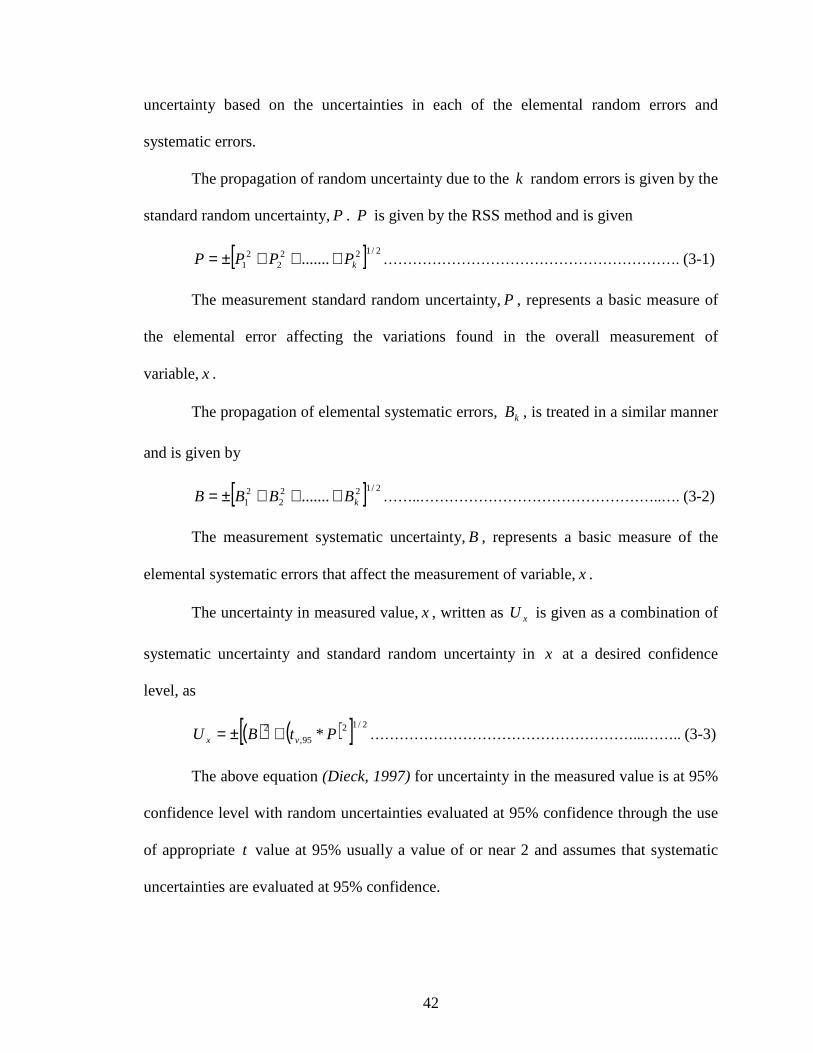
uncertainty based on the uncertainties in each of the elemental random errors and
systematic errors.
The propagation of random uncertainty due to the k random errors is given by the
standard random uncertainty,P . P is given by the RSS method and is given
[ ] 2/1222
21 ....... kPPPP +++±= ……………………………………………………. (3-1)
The measurement standard random uncertainty,P , represents a basic measure of
the elemental error affecting the variations found in the overall measurement of
variable,x .
The propagation of elemental systematic errors, kB , is treated in a similar manner
and is given by
[ ] 2/1222
21 ....... kBBBB +++±= ……..…………………………………………..…. (3-2)
The measurement systematic uncertainty,B , represents a basic measure of the
elemental systematic errors that affect the measurement of variable,x .
The uncertainty in measured value,x , written as xU is given as a combination of
systematic uncertainty and standard random uncertainty in x at a desired confidence
level, as
( ) ( )[ ] 2/1295,
2 * PtBU vx +±= ………………………………………………...…….. (3-3)
The above equation (Dieck, 1997) for uncertainty in the measured value is at 95%
confidence level with random uncertainties evaluated at 95% confidence through the use
of appropriate t value at 95% usually a value of or near 2 and assumes that systematic
uncertainties are evaluated at 95% confidence.

43
For the uncertainty in the mass flow meters, the systematic uncertainty is
represented as follows in Equation (3-4).
[ ] 2/122or resolutionaccuracymgml BBBB +±= …………………………………….....……. (3-4)
Substituting the parameters from Tables 3.1 and 3.2,
( ) 2/1222 *))60/1.0(001.0( lml mB += …………………………...…….…….... (3-5)
mgB = ( ) 2/1222 *))60/1.0(005.0( gm+ …………………………………….……(3-6)
The systematic uncertainty of the pressure sensors, temperature sensors and
density are given as 1.0=pB , 04.0=TB , and ρρ *0002.0=B .
Similarly, the standard random uncertainty is given as:
[ ] 2/122.or ityrepeatabilDSmgml PPPP +±= …………………………………..…..…… (3-7)
( ) 2/122 005.0. += mlml DSP ……………………………………………….…… (3-8)
( ) 2/122 0025.0. += mgmg DSP ……………………………………..……....…… (3-9)
The random uncertainties pP , TP , ρP of the pressure sensor, temperature sensor
and density are the standard deviations of the individual sensors denoted by pDS. , TDS. ,
ρDS. obtained from the experimental data.
Substituting, systematic uncertainty and random uncertainty for different
instruments used in the experiments, Equation (3-3) turns out to be as follows.
( ) ( )[ ] 2/1295,
2 * mlvmlml PtBU +±= ..................................................................... (3-10)
( ) ( )[ ] 2/1295,
2 * mgvmgmg PtBU +±= …………………………………………… (3-11)
( ) ( )[ ] 2/1295,
2 * pvpp PtBU +±= ………………...……………………..……... (3-12)

44
( ) ( )[ ] 2/1295,
2 * TvTT PtBU +±= ………...……….………………………...…. (3-13)
( ) ( )[ ] 2/1295,
2 * ρρρ PtBU v+±= ……………………...………………...…..… (3-14)
Equations (3-10), (3-11), (3-12), (3-13) and (3-14) represent the uncertainty of
each individual variable measured when experiments are conducted using instruments
namely, liquid and gas Micro Motion® mass flow meters, pressure transducers,
temperature sensors, respectively.
3.3.2 Uncertainty Analysis Applied to Multiphase Metering The typical multiphase meter needs to determine velocity and area occupied by
each phase in order to calculate volumetric flow rate. Hence the superficial velocity of
the liquid phase is given by
p
lsl A
Qv = ……….…………………………………………………..………. (3-15)
pl
lsl A
mv
1
=
ρ…………………………………………………………….. (3-16)
The uncertainty of the total value is sum of all the uncertainties calculated as
shown below in the equation
( )2/1
1
2
2
∂∂
= ∑=
n
iXi
i
zZ U
X
UU ………………………………………………. (3-17)
where n is the maximum number of instruments that are used in the experiments.
The uncertainty in superficial liquid velocity is calculated by substituting in the
generalized equation, Equation 3-17, and as shown in the following derived equations.

45
( )2/1
1
2
2
∂∂
= ∑=
n
iXi
i
VslVsl U
X
UU ………………………………………...…… (3-18)
( ) ( ) ( )2/1
2
2
2
2
2
2
∂∂
+
∂∂
+
∂∂
= ApAp
Vsl
l
Vslm
l
VslVsl U
UU
UU
m
UU
ll ρρ……..…… (3-19)
( )
( ) ( )
( )
2/1
2
22
2
22
22
2
2
22
1
11
11
−+
−+
=
Apl
l
p
llpl
mpl
Vsl
Um
A
UmA
UA
U
l
ρ
ρ
ρ
ρ ……………………...………...….. (3-20)
Similarly, in order to evaluate the uncertainty for superficial gas velocity, it is
necessary to convert using PVT variables as the in-situ conditions are different from the
standard conditions. Hence,
p
gsg A
Qv = ……………………………………………………………………. (3-21)
pg
sc
sc
gsg A
mv
1
=
ρρ
ρ………………………………………………………. (3-22)
pscg
sc
sc
gsg AT
T
P
Pmv
1
=
ρ…………………………………………....…… (3-23)
The uncertainty in superficial gas velocity is calculated by substituting in the
generalized equation 3-17 and as shown in the following derived equations.
( )2/1
1
2
2
∂∂
= ∑=
n
iXi
i
VsgVsg U
X
UU ………...……………………………........... (3-24)
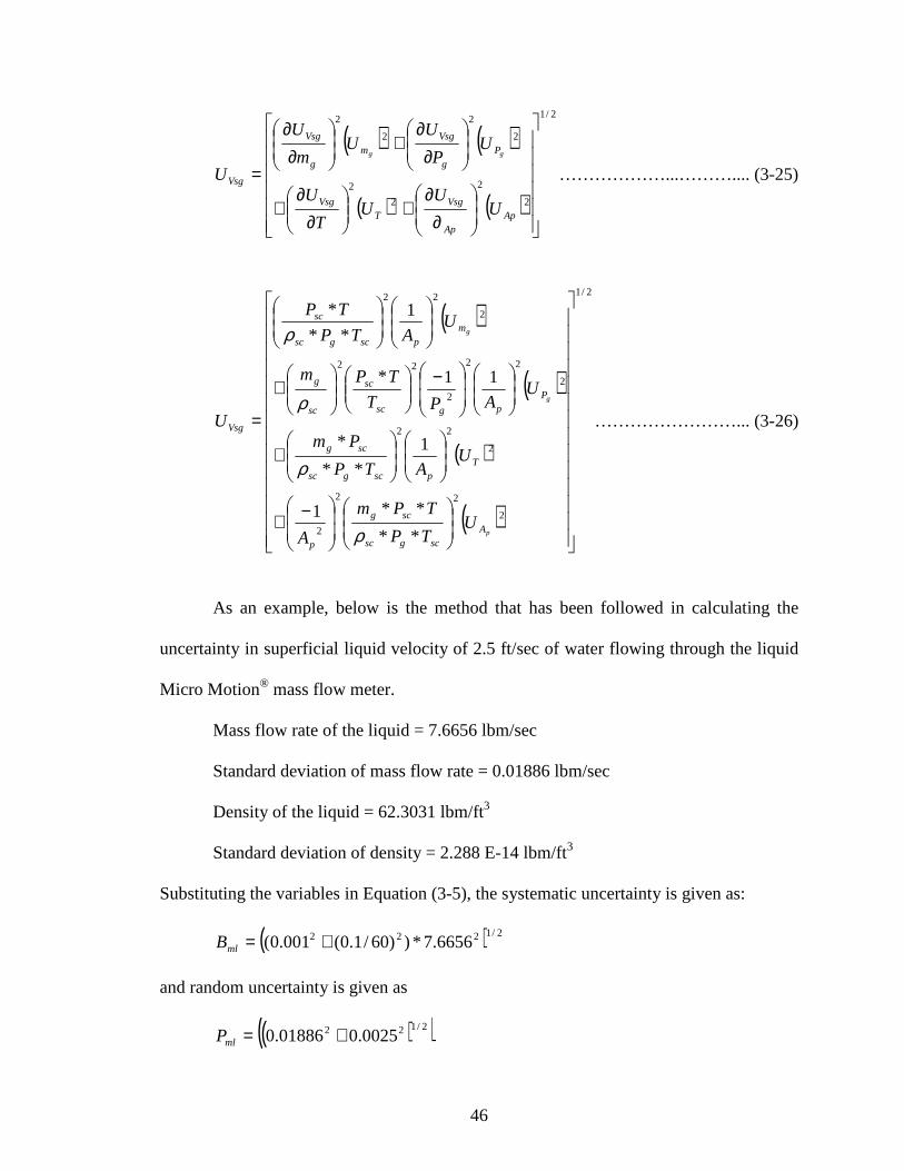
46
( ) ( )
( ) ( )
2/1
2
2
2
2
2
2
2
2
∂∂
+
∂∂
+
∂∂
+
∂∂
=
ApAp
VsgT
Vsg
Pg
Vsgm
g
Vsg
Vsg
UU
UT
U
UP
UU
m
U
Ugg
………………...……….... (3-25)
( )
( )
( )
( )
2/1
2
22
2
2
22
2
22
2
22
2
22
**
**1
1
**
*
11*
1
**
*
−+
+
−
+
=
p
g
g
Ascgsc
scg
p
Tpscgsc
scg
Ppgsc
sc
sc
g
mpscgsc
sc
Vsg
UTP
TPm
A
UATP
Pm
UAPT
TPm
UATP
TP
U
ρ
ρ
ρ
ρ
……………………... (3-26)
As an example, below is the method that has been followed in calculating the
uncertainty in superficial liquid velocity of 2.5 ft/sec of water flowing through the liquid
Micro Motion® mass flow meter.
Mass flow rate of the liquid = 7.6656 lbm/sec
Standard deviation of mass flow rate = 0.01886 lbm/sec
Density of the liquid = 62.3031 lbm/ft3
Standard deviation of density = 2.288 E-14 lbm/ft3
Substituting the variables in Equation (3-5), the systematic uncertainty is given as:
( ) 2/1222 6656.7*))60/1.0(001.0( +=mlB
and random uncertainty is given as
( )( )2/122 0025.001886.0 +=mlP

47
Substituting in Equation 3-3, uncertainty of mass flow rate of the liquid Micro Motion®
mass flow meter is then given by
( )( ) ( )( )[ ] 2/122 *2 mlmlml PBU +±=
=mlU 3.622E-04 lbm/sec
Similarly, uncertainty of the density of the liquid (from Equation (3-14))is given by
( ) ( )[ ] 2/1295,
2 14288.2*3031.62*)0002.0( −+±= EtU vlρ
02-1.25E=l
U ρ lbm/ft3
Substituting in Equation (3-20) the uncertainty for superficial liquid velocity of 2.5 ft/sec
is given as:
( )
( ) ( )
( )
2/1
222
2
2222
2
222
03031.62
6656.7
049087.0
1
0225.16656.7049087.0
1
3031.62
1
04-3.622E049087.0
1
3031.62
1
−+
−
−+
= EUVsl
005184.0=VslU ft/sec
As shown in the example above, the uncertainty analysis of the Operational
Envelop has been carried out for both light oil and heavy oil with different watercuts,
respectively. The results are shown in Tables 4.3 and 4.4 in Chapter 4.
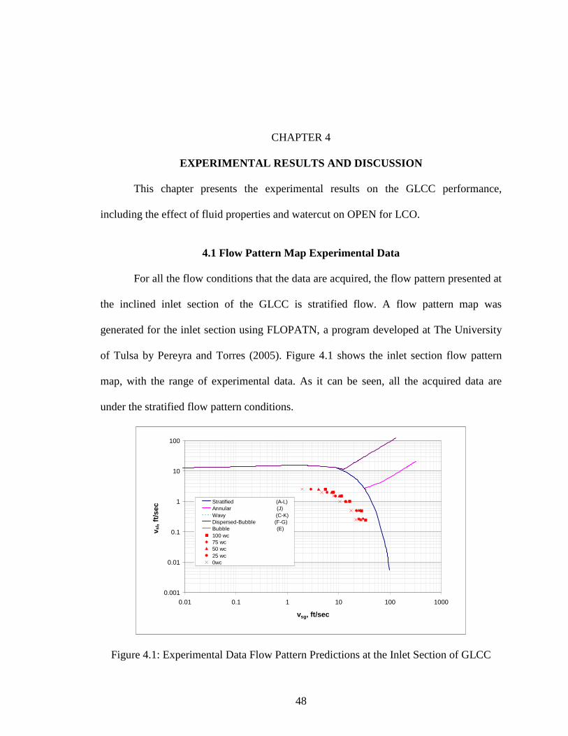
48
CHAPTER 4
EXPERIMENTAL RESULTS AND DISCUSSION
This chapter presents the experimental results on the GLCC performance,
including the effect of fluid properties and watercut on OPEN for LCO.
4.1 Flow Pattern Map Experimental Data
For all the flow conditions that the data are acquired, the flow pattern presented at
the inclined inlet section of the GLCC is stratified flow. A flow pattern map was
generated for the inlet section using FLOPATN, a program developed at The University
of Tulsa by Pereyra and Torres (2005). Figure 4.1 shows the inlet section flow pattern
map, with the range of experimental data. As it can be seen, all the acquired data are
under the stratified flow pattern conditions.
0.001
0.01
0.1
1
10
100
0.01 0.1 1 10 100 1000
vsg, ft/sec
v sl,
ft/se
c
Stratified (A-L)Annular (J)Wavy (C-K)Dispersed-Bubble (F-G)Bubble (E)100 wc75 wc50 wc25 wc0wc
Figure 4.1: Experimental Data Flow Pattern Predictions at the Inlet Section of GLCC

49
4.2 Operational Envelop
The operational envelop represents the flow conditions for initiation of LCO.
There is no LCO below the operational envelope, whereby only gas flows into the gas
leg. The operating pressure was controlled using the gas control valve and was set at a
constant pressure throughout the experiments. The working fluids are air as the gas
phase, water and mineral oil as liquid phases.
Figure 4.2 represents the experimental results of the OPEN for water (wc= 100%)
as an example. In general, at relatively lowsgv , GLCC can tolerate high liquid flow rates.
However, as sgv increases the operational envelop decreases. There are two main regions
characterizing the operational envelop namely; churn and annular. In the churn region,
characterized by low gas and high liquid rates (sgv <15 ft/sec), the liquid level is
maintained below the inlet and the gas churns the liquid up and down in the upper part of
the GLCC.
OPEN FOR LCO FOR WATER (WC=100)
0
0.5
1
1.5
2
2.5
3
0 5 10 15 20 25 30
vsg (ft/sec)
v sl
(ft/s
ec)
water
Figure 4.2: Operational Envelop for Liquid Carry-Over for Water
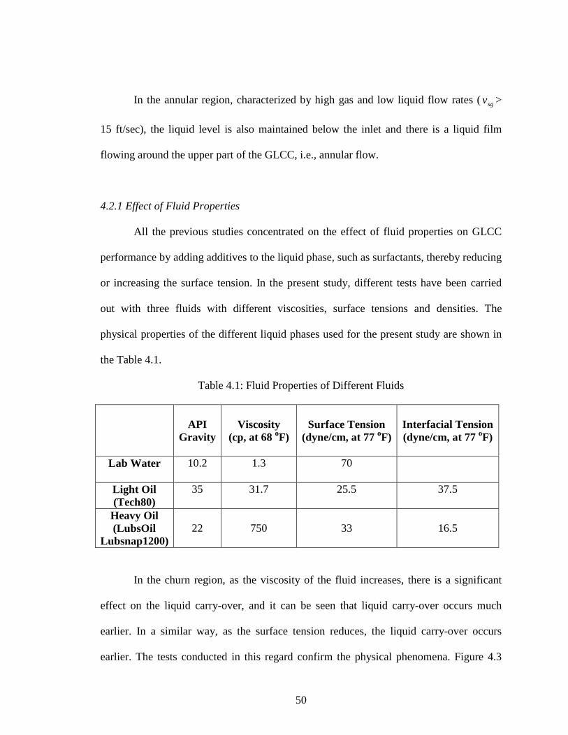
50
In the annular region, characterized by high gas and low liquid flow rates ( sgv >
15 ft/sec), the liquid level is also maintained below the inlet and there is a liquid film
flowing around the upper part of the GLCC, i.e., annular flow.
4.2.1 Effect of Fluid Properties All the previous studies concentrated on the effect of fluid properties on GLCC
performance by adding additives to the liquid phase, such as surfactants, thereby reducing
or increasing the surface tension. In the present study, different tests have been carried
out with three fluids with different viscosities, surface tensions and densities. The
physical properties of the different liquid phases used for the present study are shown in
the Table 4.1.
Table 4.1: Fluid Properties of Different Fluids
API
Gravity
Viscosity
(cp, at 68 oF)
Surface Tension
(dyne/cm, at 77 oF)
Interfacial Tension (dyne/cm, at 77 oF)
Lab Water
10.2
1.3 70
Light Oil (Tech80)
35 31.7 25.5 37.5
Heavy Oil (LubsOil
Lubsnap1200)
22
750
33
16.5
In the churn region, as the viscosity of the fluid increases, there is a significant
effect on the liquid carry-over, and it can be seen that liquid carry-over occurs much
earlier. In a similar way, as the surface tension reduces, the liquid carry-over occurs
earlier. The tests conducted in this regard confirm the physical phenomena. Figure 4.3

51
illustrates the effect of fluid properties on the operational envelop. The tests were
conducted at 25 psia.
EFFECT OF FLUID PROPERTIES
0
0.5
1
1.5
2
2.5
3
0 5 10 15 20 25 30
vsg(ft/sec)
v sl(f
t/sec
)
water
light oil
Light OilViscosity = 31.7 cpSurface Tension =
25.5 dyne/cm
WaterViscosity = 1.3 cp
Surface Tension = 70.0 dyne/cm
Figure 4.3: Effects of Fluid Properties 4.2.2 Effect of Watercut Figure 4.4 presents the operational envelop for the light oil, as a function of
watercut. The tests were conducted at 0, 25, 50, 75 and 100% watercuts. As can be seen,
the operational envelop increases as the watercut increases. It is the lowest for pure oil
and highest for pure water. The other observation that can be made is that the operational
envelop of the 75% and 100% watercuts are similar and the dominance of oil properties
is only below the 50% watercut. This emphasizes that if the fluid is water dominant, the
operational envelop will be increased and the effect of oil properties is not that
significant.
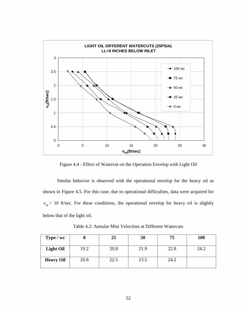
52
LIGHT OIL DIFFERENT WATERCUTS (25PSIA) LL=6 INCHES BELOW INLET
0
0.5
1
1.5
2
2.5
3
0 5 10 15 20 25 30
vsg(ft/sec)
v sl(f
t/sec
)
100 wc
75 wc
50 wc
25 wc
0 wc
Figure 4.4 - Effect of Watercut on the Operation Envelop with Light Oil
Similar behavior is observed with the operational envelop for the heavy oil as
shown in Figure 4.5. For this case, due to operational difficulties, data were acquired for
sgv > 10 ft/sec. For these conditions, the operational envelop for heavy oil is slightly
below that of the light oil.
Table 4.2: Annular Mist Velocities at Different Watercuts
Type / wc 0 25 50 75 100
Light Oil 19.2 20.8 21.9 22.8 24.2
Heavy Oil 20.8 22.5 23.5 24.2
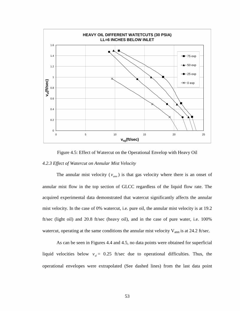
53
HEAVY OIL DIFFERENT WATETCUTS (30 PSIA) LL=6 INCHES BELOW INLET
0
0.2
0.4
0.6
0.8
1
1.2
1.4
1.6
0 5 10 15 20 25
vsg(ft/sec)
v sl(f
t/sec
)
75 exp
50 exp
25 exp
0 exp
Figure 4.5: Effect of Watercut on the Operational Envelop with Heavy Oil 4.2.3 Effect of Watercut on Annular Mist Velocity
The annular mist velocity (annv ) is that gas velocity where there is an onset of
annular mist flow in the top section of GLCC regardless of the liquid flow rate. The
acquired experimental data demonstrated that watercut significantly affects the annular
mist velocity. In the case of 0% watercut, i.e. pure oil, the annular mist velocity is at 19.2
ft/sec (light oil) and 20.8 ft/sec (heavy oil), and in the case of pure water, i.e. 100%
watercut, operating at the same conditions the annular mist velocity Vann is at 24.2 ft/sec.
As can be seen in Figures 4.4 and 4.5, no data points were obtained for superficial
liquid velocities below slv = 0.25 ft/sec due to operational difficulties. Thus, the
operational envelopes were extrapolated (See dashed lines) from the last data point
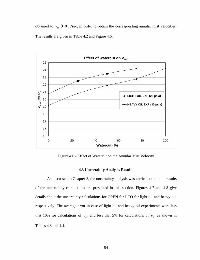
54
obtained to slv � 0 ft/sec, in order to obtain the corresponding annular mist velocities.
The results are given in Table 4.2 and Figure 4.6.
Effect of watercut on v ann
15
16
17
18
19
20
21
22
23
24
25
0 20 40 60 80 100
Watercut (%)
v ann
(ft/
sec)
LIGHT OIL EXP (25 psia)
HEAVY OIL EXP (30 psia)
Figure 4.6 - Effect of Watercut on the Annular Mist Velocity
4.3 Uncertainty Analysis Results
As discussed in Chapter 3, the uncertainty analysis was carried out and the results
of the uncertainty calculations are presented in this section. Figures 4.7 and 4.8 give
details about the uncertainty calculations for OPEN for LCO for light oil and heavy oil,
respectively. The average error in case of light oil and heavy oil experiments were less
that 10% for calculations of sgv and less that 5% for calculations of slv as shown in
Tables 4.3 and 4.4.

55
Table 4.3: Uncertainty Analysis of Light Oil with Different Watercuts
OPERATIONAL
ENVELOP ERROR ERROR IN %
sgv
(ft/sec) slv
(ft/sec) sgv
(ft/sec) slv
(ft/sec) sgv slv
1.958 2.557 ±0.228 ±5.181E-04 ±11.651 ±0.020
4.421 1.992 ±0.250 ±4.375E-04 ±5.655 ±0.022 100 wc 7.985 1.496 ±0.615 ±7.967E-04 ±7.702 ±0.053
10.685 0.990 ±0.514 ±4.093E-04 ±4.813 ±0.041 15.647 0.500 ±1.308 ±1.023E-03 ±8.360 ±0.205
17.458 0.253 ±1.233 ±5.616E-05 ±7.065 ±0.022
2.926 2.536 ±0.221 ±6.531E-04 ±7.570 ±0.026 5.874 1.975 ±0.260 ±5.410E-04 ±4.435 ±0.027
75 wc 8.747 1.492 ±0.553 ±5.765E-04 ±6.331 ±0.039 13.021 1.007 ±0.457 ±3.195E-04 ±3.513 ±0.032 17.218 0.493 ±1.135 ±5.053E-04 ±6.595 ±0.103
19.136 0.250 ±0.969 ±9.396E-05 ±5.068 ±0.038
4.191 2.517 ±0.291 ±7.781E-04 ±6.947 ±0.031 7.443 1.999 ±0.269 ±4.539E-04 ±3.618 ±0.023
50 wc 10.011 1.502 ±0.633 ±6.137E-04 ±6.328 ±0.041 14.170 1.008 ±0.429 ±2.938E-04 ±3.029 ±0.029 20.282 0.502 ±0.847 ±1.917E-04 ±4.179 ±0.038
21.306 0.256 ±0.853 ±7.467E-05 ±4.008 ±0.029
5.552 2.482 ±0.222 ±6.914E-04 ±4.012 ±0.028 7.916 2.004 ±0.237 ±1.652E-03 ±2.995 ±0.082
25 wc 11.283 1.508 ±0.677 ±4.525E-04 ±6.003 ±0.030 16.922 1.011 ±0.496 ±2.277E-04 ±2.931 ±0.023 22.278 0.505 ±0.561 ±1.277E-04 ±2.521 ±0.025
22.540 0.254 ±1.401 ±1.055E-04 ±6.219 ±0.042
5.466 2.532 ±0.188 ±6.777E-04 ±3.439 ±0.027 7.816 2.000 ±0.204 ±4.461E-04 ±2.614 ±0.022
0 wc 11.645 1.503 ±0.690 ±6.664E-04 ±5.931 ±0.044 16.677 1.002 ±0.696 ±4.079E-04 ±4.174 ±0.041 23.538 0.494 ±0.479 ±1.208E-04 ±2.035 ±0.024
24.058 0.248 ±0.658 ±1.656E-04 ±2.735 ±0.067

56
Table 4.4: Uncertainty Analysis of Heavy Oil with Different Water Cuts
OPERATIONAL
ENVELOP ERROR ERROR IN %
sgv
(ft/sec) slv
(ft/sec) sgv
(ft/sec) slv
(ft/sec) sgv slv
10.663 1.494 ±0.235 ±2.354E-04 ±2.206 ±0.016 75 wc 18.144 1.004 ±0.409 ±1.787E-04 ±2.256 ±0.018
21.184 0.512 ±0.803 ±1.139E-04 ±3.791 ±0.022 23.070 0.256 ±1.002 ±1.072E-04 ±4.341 ±0.042
9.765 1.498 ±0.235 ±3.365E-04 ±2.403 ±0.022
16.123 1.000 ±0.364 ±2.189E-04 ±2.260 ±0.022 50 wc 20.486 0.492 ±0.561 ±1.002E-04 ±2.737 ±0.020
22.444 0.253 ±0.561 ±7.315E-05 ±2.499 ±0.029
8.996 1.473 ±0.190 ±3.606E-04 ±2.112 ±0.024 13.781 0.962 ±1.176 ±4.583E-04 ±8.537 ±0.048
25 wc 18.824 0.497 ±0.403 ±1.137E-04 ±2.142 ±0.023 21.453 0.250 ±0.679 ±5.366E-05 ±3.163 ±0.021
9.484 0.972 ±0.465 ±8.618E-04 ±4.901 ±0.089
0 wc 16.301 0.498 ±0.262 ±1.092E-04 ±1.604 ±0.022 19.255 0.253 ±0.594 ±5.147E-05 ±3.086 ±0.020

57
UNCERTAINTY OF OPEN FOR LIGHT OIL AT DIFFERENT WATER CUTS
0
0.5
1
1.5
2
2.5
3
0 5 10 15 20 25 30
vsg (ft/sec)
v sl (f
t/sec
)0 WC
25 WC
50 WC
75 WC
100 WC
Figure 4.7: Uncertainty Analysis of Operational Envelop for Light Oil with Different Watercuts
UNCERTAINTY OF OPEN FOR HEAVY OIL AT DIFFERENT WATER CUTS
0
0.2
0.4
0.6
0.8
1
1.2
1.4
1.6
0 5 10 15 20 25 30vsg (ft/sec)
v sl (f
t/sec
)
0 WC
25 WC
50 WC
75 WC
Figure 4.8: Uncertainty Analysis of Operational Envelop for Heavy Oil with Different Watercuts

58
CHAPTER 5
MECHANISTIC MODELING
This chapter presents the new mechanistic model for predicting the GLCC
operational envelop for liquid carry-over for three phase flow. It is necessary to analyze
the performance of various integral parts of the GLCC, including the inlet of the GLCC
followed by the nozzle analysis and finally the GLCC body, in order to evaluate the
overall performance of the GLCC. These are covered in the following sections.
5.1 Inlet Analysis
The complex flow patterns that take place in the inlet as well as in the GLCC
make it difficult to develop accurate performance predictions. There are different flow
patterns that occur in the upper part of the GLCC namely slug/churn, annular mist, and
swirling churn. The flow in the lower part generally consists of liquid vortex with a gas
core filament. The inlet section determines the incoming gas-liquid distribution and the
initial tangential velocities of the two phases in the GLCC. The flow patterns at the inlet
of the GLCC are primarily of stratified, slug, dispersed bubble or annular flow.
Investigations conducted by Kouba et al. (1995) have demonstrated that an
inclined inlet improves the performance of GLCC as it promotes stratification and
provides preliminary separation at the inlet unlike the conventional vertical separator
which traditionally uses horizontal inlet. Also, the downward inclination causes the liquid

59
stream to spiral below the inlet of the GLCC preventing the liquid from blocking the flow
of gas in to the upper part of the GLCC.
A sector-slot/plate configuration is employed for inlet nozzle in to the GLCC as
shown in Figure 5.1.. For the above mentioned configuration the sectional shape of the
nozzle is approximated by an equivalent rectangle for simplification. The slot area at
location 2 is given by
( )heqv
inslot LW
AA =
×=
100
Reduction of % )( dLh < …………...………….. (5-1)
where inA is the cross-sectional area of the inlet region at section 1, eqvW is the equivalent
width of the rectangular nozzle (which has the same area of cross-section as that of the
sector-slot nozzle) and hL is the height of the sector-slot perpendicular to the axis of the
inlet. It may be noted that the height of the inlet slot on the GLCC body is
θcos/'hh LL = , as shown in the Figure 5.1.
Figure 5.1: Schematic View of the Inclined Inlet of the GLCC
din 1
2
θ
NOZZLE
Lh L`h
INLET NOZZLE
GLCC
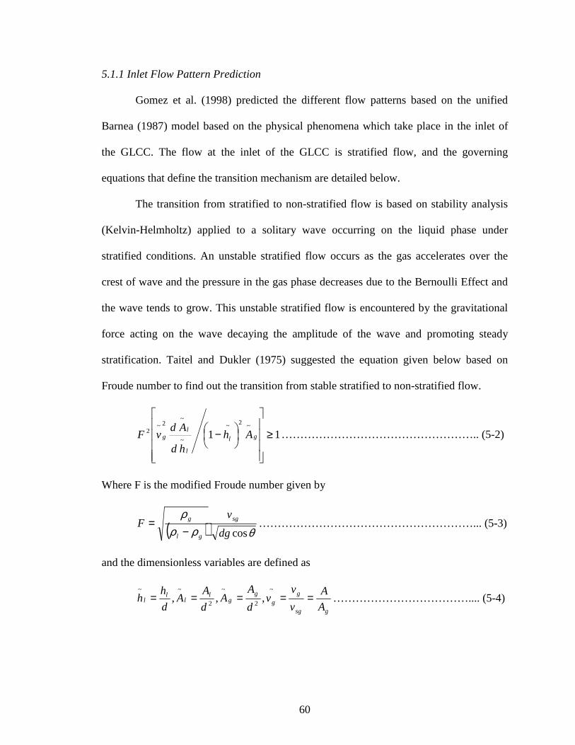
60
5.1.1 Inlet Flow Pattern Prediction
Gomez et al. (1998) predicted the different flow patterns based on the unified
Barnea (1987) model based on the physical phenomena which take place in the inlet of
the GLCC. The flow at the inlet of the GLCC is stratified flow, and the governing
equations that define the transition mechanism are detailed below.
The transition from stratified to non-stratified flow is based on stability analysis
(Kelvin-Helmholtz) applied to a solitary wave occurring on the liquid phase under
stratified conditions. An unstable stratified flow occurs as the gas accelerates over the
crest of wave and the pressure in the gas phase decreases due to the Bernoulli Effect and
the wave tends to grow. This unstable stratified flow is encountered by the gravitational
force acting on the wave decaying the amplitude of the wave and promoting steady
stratification. Taitel and Dukler (1975) suggested the equation given below based on
Froude number to find out the transition from stable stratified to non-stratified flow.
11~2~
~
~2~
2 ≥
− gl
l
lg Ah
hd
AdvF …………………………………………….. (5-2)
Where F is the modified Froude number given by
( ) θρρρ
cosdg
vF sg
gl
g
−= …………………………………………………... (5-3)
and the dimensionless variables are defined as
gsg
gg
gg
ll
ll
A
A
v
vv
d
AA
d
AA
d
hh =====
~
2
~
2
~~
,,, ……………………………….... (5-4)

61
5.1.2 Nozzle Analysis for Stratified Flow A schematic of the stratified flow in the inlet of the GLCC is shown below. As
shown in Figure 5.2 for stratified conditions in the inlet, the liquid level height increases
to 2lh as a result of the reduction in the cross-sectional area in the nozzle whereas the
liquid level height at the inlet i.e. section 1 is 1lh . The corresponding liquid and gas flow
velocities are lv and gv , respectively. As a result of the reduction in area that is present,
the velocities of both gas and liquid are greater at section 2 than at section1.
Figure 5.2: Stratified Flow Nomenclature and Geometry at the Inlet
Taitel and Dukler(1975) model which is based on the momentum (force) balance
for the liquid and gas phases is used to determine the upstream flow parameters, namely,
liquid velocity ( 1lv ), gas velocity ( 1gv ), and liquid level height ( 2lh ). The combined
momentum equation for the two phases eliminating the pressure gradient is obtained as
follows.
1
2
θ
d
hl1 vg1
hl2
vl1
vg2
vl2
Lh

62
( ) 0sin11 =−+
++− θρρτττ g
AAS
A
S
A
Sgl
glii
l
lwi
g
gwg …………………….. (5-5)
The combined momentum equation is an implicit equation for hl, the liquid level in the
inlet pipe which combines all the forces that act on the liquid and gas phases. Different
force variables and geometric parameters are necessary to be determined in order to solve
the equation for hl, the liquid level in the pipe. The interfacial shear stresses and wall
shear stresses are given for each phase as:
2
2ll
lwl
vf
ρτ = ……………………………………………………………….... (5-6)
2
2gg
gwg
vf
ρτ = ……………………………………………………………….. (5-7)
( )2
2lgg
ii
vvf
−=
ρτ ………………………………………………....………. (5-8)
Gomez (1998) determined the liquid wall friction factor, f1 incorporating the gas
and liquid flow rates based on the correlation developed by Liang-Biao and Aziz (1996).
Blasius equation is used to calculate the gas wall friction factor fg. The interfacial factor fl
is calculated using the Baker et al. (1988) equations. The interface velocity is iv (<< gv ).
All the geometric parameters are functions of the equilibrium liquid height hl. The insitu
areas of the gas and liquid phasesgA , lA and lS , gS , the wetted perimeters of interface,
liquid and gas respectively are included in this equations.
The actual liquid and gas velocities at section1 are thus defined by the ratio of
flow rate to the corresponding phase area as follows.
l
ll A
qv =
1……………………………………………………………………..... (5-9)
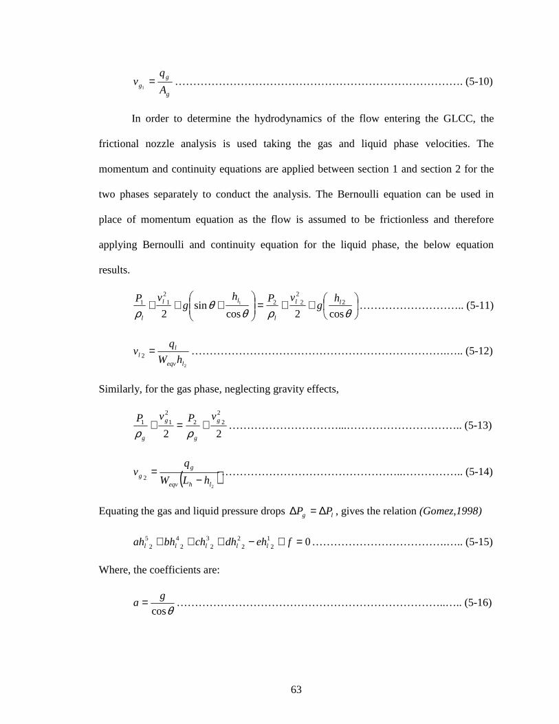
63
g
gg A
qv =
1……………………………………………………………………. (5-10)
In order to determine the hydrodynamics of the flow entering the GLCC, the
frictional nozzle analysis is used taking the gas and liquid phase velocities. The
momentum and continuity equations are applied between section 1 and section 2 for the
two phases separately to conduct the analysis. The Bernoulli equation can be used in
place of momentum equation as the flow is assumed to be frictionless and therefore
applying Bernoulli and continuity equation for the liquid phase, the below equation
results.
++=
+++
θρθθ
ρ cos2cossin
222
221
21 1 ll
l
ll
l
hg
vPhg
vP……………………….. (5-11)
2
2leqv
ll hW
qv = …………………………………………………………….….. (5-12)
Similarly, for the gas phase, neglecting gravity effects,
222
2
21
2
1 g
g
g
g
vPvP+=+
ρρ…………………………...………………………….. (5-13)
( )2
2lheqv
gg hLW
qv
−= …………………………………………..…………….. (5-14)
Equating the gas and liquid pressure drops lg PP ∆=∆ , gives the relation (Gomez,1998)
021
22
23
24
25 =+−+++ fehdhchbhah lllll ……………………………….….. (5-15)
Where, the coefficients are:
θcos
ga = ………………………………………………………………..….. (5-16)

64
θθθ
ρρ
cos
2
cossin
221
21
21 hllg
l
g gLhg
vvb −
+−−
= ……………………….…….. (5-17)
hgl
ghh
lhl Lv
gLL
hgLvc 2
1
212
1 coscossin2
−+
++=
ρρ
θθθ ………...………….... (5-18)
2
221
221
2
222
1 2cossin
22
1
eqv
lh
lhl
eqv
ghg
l
g
W
qL
hg
Lv
W
qLvd +
+−−
−
=
θθ
ρρ
………..... (5-19)
2
2
eqv
hl
W
Lqe = …………………………………………………………………..... (5-20)
2
22
2 eqv
hl
W
Lqf = …………………………………………………………………... (5-21)
The Newton-Raphson method is used to solve the 5th order polynomial obtained
in Equation (5-15). The numerical solutions of the third order polynomial representing an
equivalent open channel flow are used as initial value for the variables in order to ensure
numerical convergence of the final iterative solution. This approach is justified, as the
solution for stratified flow is physically similar to that of an open channel flow (hydraulic
jump case) incorporating the gas phase effects.
The solutions of the equations yield the liquid level at the nozzle 2lh which allows
the calculation of the corresponding gas and liquid velocities respectively. These
velocities at the nozzle are oriented along the axis of the inclined inlet. The tangential
velocities, components of the nozzle exit velocities perpendicular to the GLCC axis are
responsible for the swirling motion inside the GLCC. Therefore, the tangential liquid and
gas velocities at GLCC entrance can be calculated from the above equation, as follows.
θcos2 eqvl
ltl Wh
qv = ……...……………………………………………….…... (5-22)

65
( ) θcos2 eqvlslot
gtg WhA
qv
−= ………………………………………………….. (5-23)
Figure 5.3: Velocity Components at the Inlet of the GLCC
5.2 Zero-Net Liquid Holdup
A modified Taylor bubble rise velocity expression for Zero-Net liquid flow is
developed (Chirinos et al., 2000) to calculate the gas velocity in the upper leg of the
GLCC, assuming a churn flow in the upper leg.
sl
glsggo gDvCv
−+=
ρρρ
35.00 …………………………………….….. (5-24)
The constant for the flow coefficient 0C is assumed for slug/churn flow, as given by
0C = 1.15………………………………………………………………...….. (5-25)
The liquid hold up in the upper leg (Chirinos et al., 2000) is given by
−
−=
top
d
go
sglo L
L
v
vH 11 …………………………..……………………….. (5-26)
where 1gL is the total height of the upper leg of GLCC above the inlet. Churn flow occurs
only in the lower region, right above the inlet, while at the top region, liquid is present
primarily in the form of droplets. The length of the droplet region, dL , can be determined
from a simplified droplet ballistic analysis. It is equal to the trajectory length of a fine
droplet before it hits the wall, assuming that the gas void fraction in this region is
V tangential
V inlet
θ
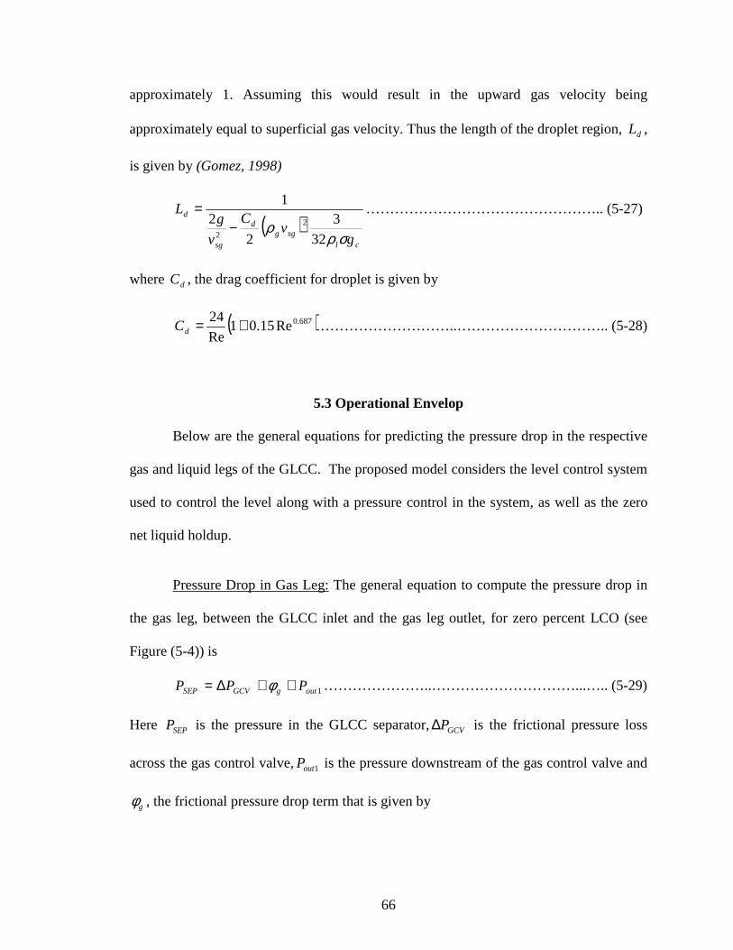
66
approximately 1. Assuming this would result in the upward gas velocity being
approximately equal to superficial gas velocity. Thus the length of the droplet region, dL ,
is given by (Gomez, 1998)
( )cl
sggd
sg
d
gv
C
v
gL
σρρ
32
3
2
21
2
2−
= ………………………………………….. (5-27)
where dC , the drag coefficient for droplet is given by
( )687.0Re15.01Re
24 +=dC ………………………..………………………….. (5-28)
5.3 Operational Envelop
Below are the general equations for predicting the pressure drop in the respective
gas and liquid legs of the GLCC. The proposed model considers the level control system
used to control the level along with a pressure control in the system, as well as the zero
net liquid holdup.
Pressure Drop in Gas Leg: The general equation to compute the pressure drop in
the gas leg, between the GLCC inlet and the gas leg outlet, for zero percent LCO (see
Figure (5-4)) is
1outgGCVSEP PPP ++∆= φ …………………..…………………………...….. (5-29)
Here SEPP is the pressure in the GLCC separator,GCVP∆ is the frictional pressure loss
across the gas control valve,1outP is the pressure downstream of the gas control valve and
gφ , the frictional pressure drop term that is given by
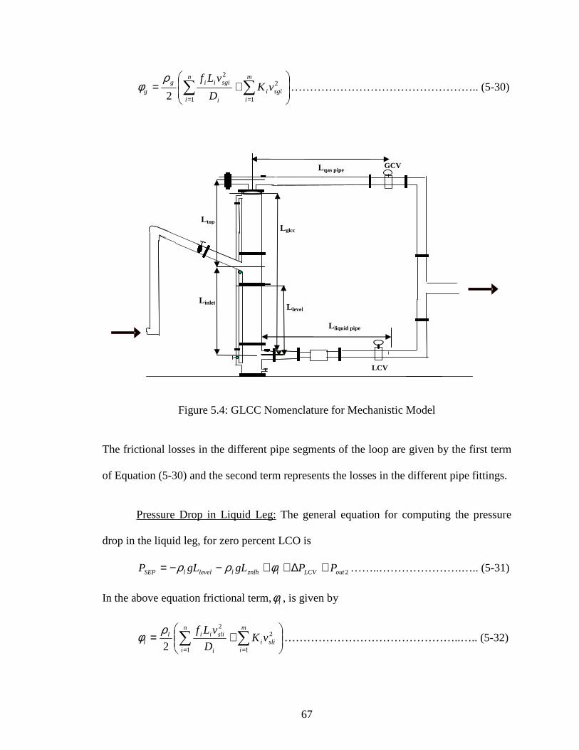
67
+= ∑∑
==
m
isgii
n
i i
sgiiigg vK
D
vLf
1
2
1
2
2
ρφ ………………………………………….. (5-30)
Figure 5.4: GLCC Nomenclature for Mechanistic Model
The frictional losses in the different pipe segments of the loop are given by the first term
of Equation (5-30) and the second term represents the losses in the different pipe fittings.
Pressure Drop in Liquid Leg: The general equation for computing the pressure
drop in the liquid leg, for zero percent LCO is
2outLCVlznlhllevellSEP PPgLgLP +∆++−−= φρρ ……..………………….….. (5-31)
In the above equation frictional term,lφ , is given by
+= ∑∑
==
m
islii
n
i i
sliiill vK
D
vLf
1
2
1
2
2
ρφ ………………………………………..….. (5-32)
GCV
LCV
L liquid pipe
L inlet
L top L glcc
L level
L qas pipe

68
The frictional losses in the different pipe segments of the loop are given by the first term
of Equation (5-32) and the second term represents the losses in the different pipe fittings.
Assumptions:
• Liquid level is fixed at 6” below the inlet in the GLCC (3.5’liquid column
height). The set point of the liquid level is modified based on the watercut
of the incoming liquid stream.
• Gas control valve (GCV) is maintaining the required pressure in the
GLCC.
• Liquid control valve (LCV) acts to maintain the liquid level in the GLCC.
Following is the model for the prediction of the different regions of the OPEN for LCO.
5.3.1 Flooding Point As the name signifies, this point is a limiting condition in the OPEN for LCO in GLCC,
which occurs when no gas flows into the GLCC, i.e. superficial gas velocity is zero
( 0=sgv ). For this condition the control system is out of bound; the gas control valve is
saturated, i.e. fully closed as there is no gas flowing in to the system; the liquid control
valve is saturated too, i.e. fully open in order to let the maximum flow of liquid through
the liquid leg.
Under the flooding conditon, as there is no gas flow in to the GLCC and the gas
control valve and the liquid control valve are saturated, LCVP∆ and GCVP∆ and gφ can be
neglected. If these are taken into consideration into Equation 5-31, the pressure drop
equation in the liquid leg becomes
LCVleqvloutSEP PgLPP ∆++−=− φρ2 ……………...…………………..…….. (5-33)

69
Similarly, for the gas leg
0==∆ gGCVP φ ……………………………………………………….…….. (5-34)
In reality, the gas valve is closed and the equation for the gas leg is not used at all.
Assuming 1outP = 2outP , for this case from Equation 5-33, it is evident that the gravitational
pressure head should be equal to the frictional losses in the GLCC and the liquid leg, i.e.,
topinleteqv LLL += …………………………………………………………….. (5-35)
( )WcWc owl −+= 1ρρρ …………………………………………………..….. (5-36)
5.3.2 Churn Region
In this region, there is a certain amount of gas flowing into the system and liquid
churns up and down in the top section of the GLCC. The gravity head as a result of the
churning is given by znlhl gLρ .
Equation (5-29) for the pressure drop in the gas leg can be written as
gGCVoutSEP PPP φ+∆=− 1 ………………………………………………….. (5-37)
where the pressure in the GLCC, SEPP is maintained constant throughout the study and
1outP remains the same downstream of the control valve.
In the case of liquid leg, as the superficial gas velocity increases, the gravity
pressure head due to the zero net liquid holdup reduces, and the LCV acts as to
accommodate for the pressure loss. For a steady-state flow condition, when the
superficial gas velocity flowing into the system is increased, the LCV starts to close as
the hydrostatic head reduces. Hence for this case, it can be assumed that the K value of
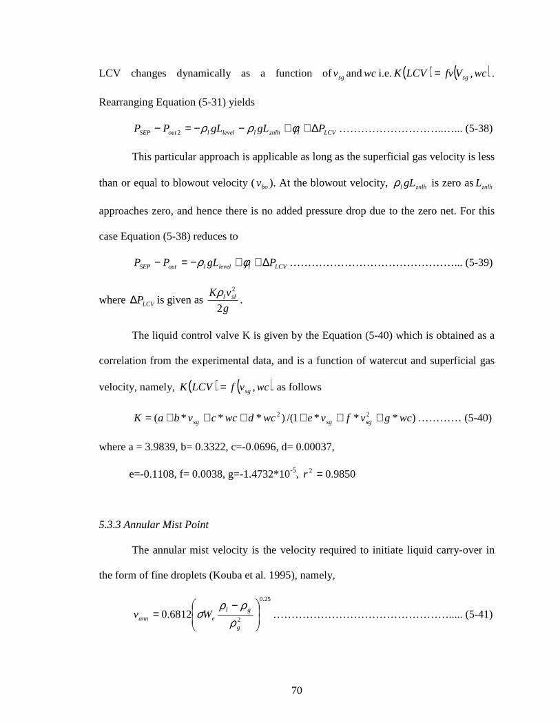
70
LCV changes dynamically as a function ofsgv andwc i.e. ( ) ( )wcVfvLCVK sg,= .
Rearranging Equation (5-31) yields
LCVlznlhllevelloutSEP PgLgLPP ∆++−−=− φρρ2 ………………………..…... (5-38)
This particular approach is applicable as long as the superficial gas velocity is less
than or equal to blowout velocity (bov ). At the blowout velocity, znlhl gLρ is zero as znlhL
approaches zero, and hence there is no added pressure drop due to the zero net. For this
case Equation (5-38) reduces to
LCVllevelloutSEP PgLPP ∆++−=− φρ ………………………………………... (5-39)
where LCVP∆ is given as g
vK sll
2
2ρ.
The liquid control valve K is given by the Equation (5-40) which is obtained as a
correlation from the experimental data, and is a function of watercut and superficial gas
velocity, namely, ( ) ( )wcvfLCVK sg,= as follows
)***1/()***( 22 wcgvfvewcdwccvbaK sgsgsg ++++++= ………… (5-40)
where a = 3.9839, b= 0.3322, c=-0.0696, d= 0.00037,
e=-0.1108, f= 0.0038, g=-1.4732*10-5, 9850.02 =r
5.3.3 Annular Mist Point
The annular mist velocity is the velocity required to initiate liquid carry-over in
the form of fine droplets (Kouba et al. 1995), namely,
25.0
26812.0
−=
g
gleann Wv
ρρρ
σ …………………………………………..... (5-41)

71
where eW is the Weber number (approximately equal to 8.0 for very fine droplets). The
two phase mixture density and equivalent surface tension are given, respectively, by
Equations (5-42) and (5-43).
( )WcWc owl −+= 1ρρρ …………………………………………………..... (5-42)
( )WcWc owl −+= 1σσσ ………………………………………………...….. (5-43)
Thus, the present model incorporates the effect of watercut and fluid properties
based on the zero net liquid flow analysis and annular mist velocities along with control
scenario.
Procedure for Operational Envelop Determination: The following input variables
are used to calculate the liquid carry-over operational envelop for 3-phase flow in GLCC.
• Specific gravity of oil ( - )
• Specific gravity of water( - )
• Density of water( lbm/ft3)
• Watercut ( - )
• Viscosity of oil (cp)
• Viscosity of water (cp)
• Diameter of GLCC (inches)
• Diameter of the piping (inches)
• Bottom length of GLCC (ft)
• Surface tension of water (dyne/cm)
• Surface tension of oil (dyne/cm)

72
Step 1: Assume a superficial gas velocity.
Calculate the blow out velocity using Equation (5-27) and assuming dL = topL (Obtained
from Equation (5-26) when 0=loH )
If the assumed superficial gas velocity is less than blow out velocity, calculate the
maximum liquid hold up in the upper section of the GLCC using zero net liquid holdup.
If the assumed superficial gas velocity is greater than blowout velocity, calculate annular
mist velocity and the operational envelop is a linear line between blow out and annular
mist velocity.
Inputs: Drag coefficient, dC , Flow coefficient, oC , Density of gas, gρ , Density of liquid,
lρ , Surface tension,lσ
Figure 5.5: Procedure to Determine the LCO Operational Envelop (Part 1) Outputs: Zero Net Liquid Hold up & Height
Assume Vsg
If Vsg<Vbo
Blowout (Vbo) Equation (5-27) = Lg
(Where Ld =Lg(topsection))
Calculate the Zero Net Liquid Holdup & Height Equation (5-26)
Join with Linear Line
between Vbo and
Vann
Calculate Annular Mist Velocity (Vann) using
Equation (5-41)
NO
YES

73
Step2:
Substitute the zero net liquid holdup height and K of the liquid control valve in the
pressure drop equation of the liquid leg. In order to satisfy this Equation (5-38), a value
of slv is guessed in order to solve. The value of superficial liquid velocity, slv , is
incremented in steps and the pressure drop equation is satisfied.
Inputs: Zero net liquid hold up & Height, Control valve K, Psep, Pout, Liquid level Set
point, Frictional losses, Density of the liquid
Figure 5.6: Procedure to Determine the LCO Operational Envelop (Part 2)
Output: Final slv on OPEN for LCO for a particular sgv
Repeat the procedure above described incrementing the sgv until it reachesbov .
Input Variables Psep, Pout, Liquid
Level(set point)
Substitute the Zero Net liquid height
(Lznlh) in to pressure drop
Equation (5-38)
Zero Net Liquid
Holdup & Height
Calculate K from Equation
5-40
Final Vsl for 0% LCO
operational envelop for
that Vsg
Satisfy
Equation 5-38
Initial Vsl
YES Increment Vsl
NO

74
CHAPTER 6
COMPARISON OF MODEL PREDICTION WITH EXPERIMENTAL DA TA This chapter includes comparison between the experimental data for the
operational envelop for liquid carryover and the model predictions.
6.1 Prediction of Annular Mist Velocity
The watercut has a significant effect on the annular mist velocity, as can be seen
from the experimental results given earlier. Figure 6.1 shows the comparison of modeling
predictions (Equations (5-40) to (5-42)) and experimental data results of annular mist
velocities for both light oil and heavy oil. The model predictions are plotted with solid
symbols highlighting the watercut. The experimental data are shown with unfilled
symbols. The maximum error seen in the prediction of annular mist velocity is less than
4% which occurs for 100% watercut.
6.2 Prediction of Operational Envelop (OPEN) Comparison between the experimental results for the OPEN for LCO and the
model predictions are given in Figure 6.2 for light oil. These results are for varying
watercuts from 0% to 100% i.e. operational envelops from pure oil to pure water. The
mechanistic model predictions are shown with different line types. The experimental
results are shown as markers. The results are for 25 psig and 77oF with surface tension of

75
25.5 and 70 dyne/cm and viscosity of 31.7 and 1.3 cp for light oil and water, respectively.
Fair agreement is observed in the comparison.
Effect of watercut on v ann
15
17
19
21
23
25
27
0 20 40 60 80 100
Watercut (%)
v ann
(ft/
sec)
LIGHT OIL EXPLIGHT OIL modelHEAVY OIL MODELHEAVY OIL EXP
Figure 6.1: Comparison of Annular Mist Velocities for Light Oil and Heavy Oil
COMPARISON OF OPEN FOR LIGHT OIL DIFFERENT WATERCUT S
0
0.5
1
1.5
2
2.5
3
0 5 10 15 20 25 30
vsg (ft/sec)
v sl (
ft/se
c)
100 exp75 exp50 exp25 exp0 exp0 model25 model50 model75 model100 model
Figure 6.2: Comparison of Experimental Data with Modeling Predictions for Light Oil

76
Figure 6.3 gives a similar comparison between experimental results of OPEN for
LCO and the model predictions for heavy oil. The model predictions are shown with
different line types. The experimental results are plotted as unfilled markers for different
watercuts. The experimental data were acquired at 30 psig and 100oF and the viscosity of
the pure oil is 200 cp and surface tension of 33 dyne/cm. Again, fair agreement is
observed in the comparison and on the overall model predictions are conservative.
COMPARISON OF OPEN FOR HEAVYOIL DIFFERENT WATERCUTS
0
0.5
1
1.5
2
2.5
0 5 10 15 20 25 30
vsg (ft/sec)
v sl (f
t/sec
)
75 exp
50 exp
25 exp
0 exp
0 model
25 model
50 model
75 model
Figure 6.3: Comparison of Experimental Data and Modeling Predictions for Heavy Oil

77
CHAPTER 7
CONCLUSIONS AND RECOMMENDATIONS
This chapter presents the conclusions of this study and also gives
recommendations for future work.
7.1 Conclusions
• Experimental data were acquired in a 3” diameter GLCC for the operational
envelop for liquid carry-over (OPEN for LCO) under three-phase flow. Both light
oil and heavy oil and different watercuts (0-100%) were utilized and the liquid
level was controlled at 6” below the GLCC inlet.
• Experimental data were also acquired for annular mist velocities for different
watercuts (0-100%) for both light oil and heavy oil.
• A significant effect of watercut on the OPEN for LCO for three phase flow has
been observed. As the watercut reduces, the OPEN for LCO reduces. Similarly,
reduction in water cut also reduces annular mist velocity.
• The operational envelop for heavy oil reduces as compared to light oil which
could be due the effect of viscosity and density.
• The annular mist velocity increases with surface tension. For light oil (σ =25.5
dyne/cm), annv = 19.2 ft/sec and for heavy oil (σ =33 dyne/cm), annv = 20.8 ft/sec.

78
• A modified mechanistic model for the prediction of OPEN for LCO for three
phase flow is presented. The proposed model incorporates the liquid level and
pressure control configuration, as well as the effect of watercut and fluid
properties. Good agreement is observed between the predicted results and the
experimental data.
7.2 Recommendations
• Carryout experiments for the OPEN of heavy oil for Vsg < 10 ft/sec in the churn
region.
• Obtain actual LCO data for three-phase flow, beyond the OPEN.
• Obtain three phase flow experimental data under high pressure conditions.
• Obtain zero-net liquid hold up data for different watercuts and refine the model as
needed.
• Obtain zero-net liquid hold up data for different watercuts under flowing
conditions and incorporate in the developed model.
• Develop a mechanistic model for the pressure drop equation for generalized
control valves employed in the field.
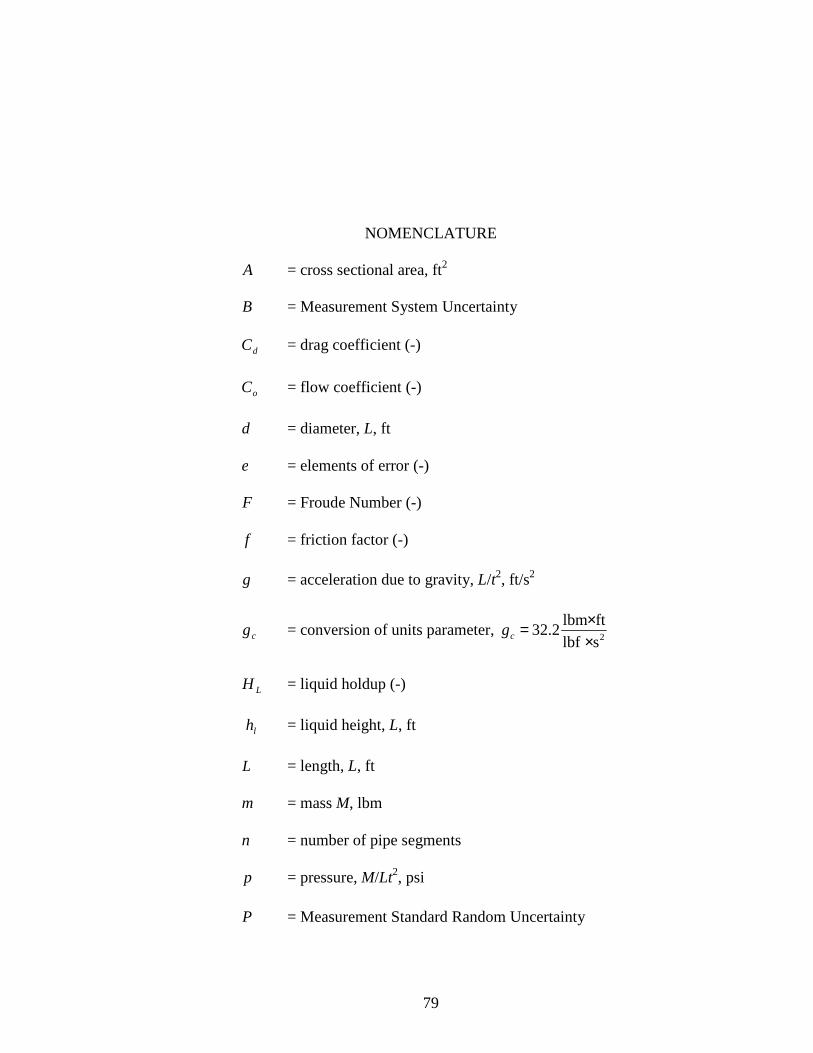
79
NOMENCLATURE
A = cross sectional area, ft2
B = Measurement System Uncertainty
dC = drag coefficient (-)
oC = flow coefficient (-)
d = diameter, L, ft
e = elements of error (-)
F = Froude Number (-)
f = friction factor (-)
g = acceleration due to gravity, L/t2, ft/s2
cg = conversion of units parameter, 2slbfftlbm
32.2××=cg
LH = liquid holdup (-)
lh = liquid height, L, ft
L = length, L, ft
m = mass M, lbm
n = number of pipe segments
p = pressure, M/Lt2, psi
P = Measurement Standard Random Uncertainty
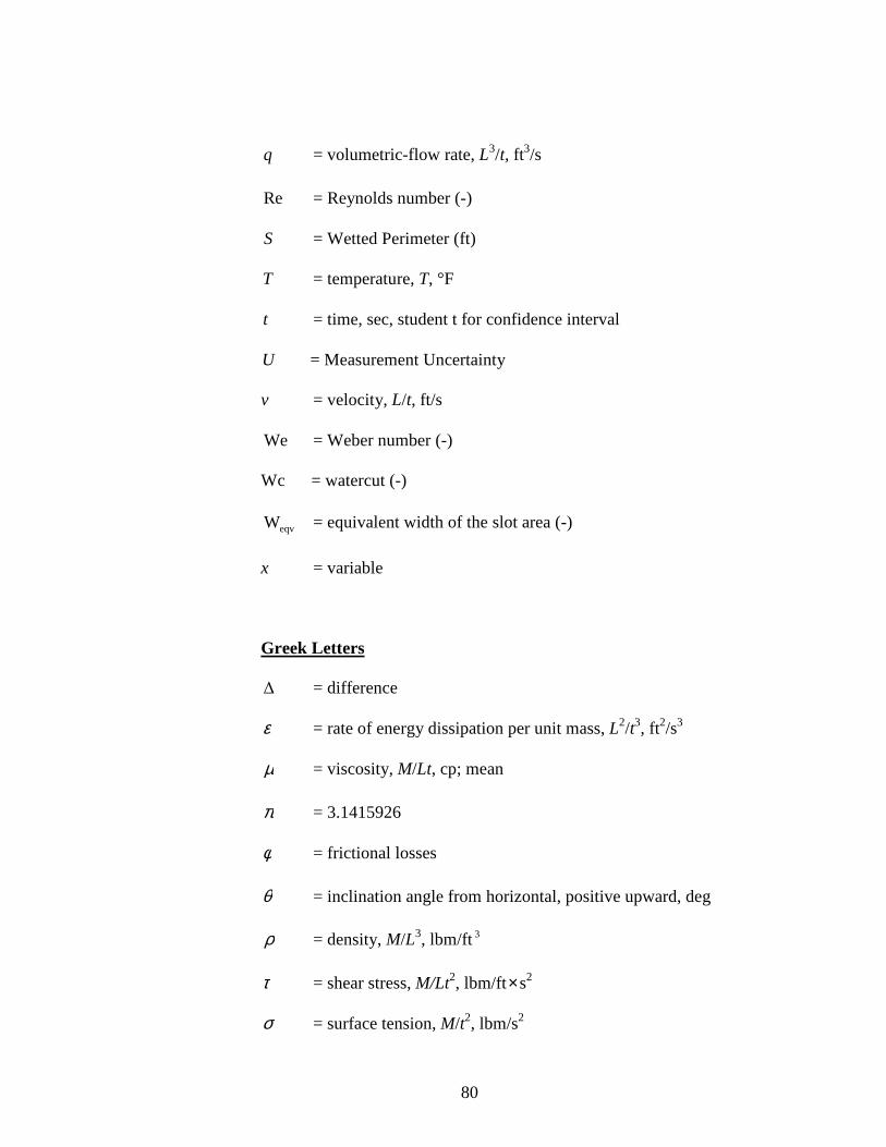
80
q = volumetric-flow rate, L3/t, ft3/s
Re = Reynolds number (-)
S = Wetted Perimeter (ft)
T = temperature, T, °F
t = time, sec, student t for confidence interval
U = Measurement Uncertainty
v = velocity, L/t, ft/s
We = Weber number (-)
Wc = watercut (-)
eqvW = equivalent width of the slot area (-)
x = variable
Greek Letters
∆ = difference
ε = rate of energy dissipation per unit mass, L2/t3, ft2/s3
µ = viscosity, M/Lt, cp; mean
π = 3.1415926
φ = frictional losses
θ = inclination angle from horizontal, positive upward, deg
ρ = density, M/L3, lbm/ft3
τ = shear stress, M/Lt2, lbm/ft×s2
σ = surface tension, M/t2, lbm/s2

81
..DS = Standard Deviation
Subscripts
ann = annular mist
co = carry-over
eqv = equivalent
g = gas
GCV = gas control valve
h = height of the sector slot
in = inlet
k = number of elements of error
l = liquid
liq = liquid
level = GLCC liquid level
LCV = liquid control valve
n = number of instruments; Number of pipe sections
m = number of fittings
out1 = reference (outside GCV)
out2 = reference (outside LCV)
pipe = annular mist
sep = separator
sg = superficial gas
sl = superficial liquid
top = top section

82
znlh = Zero Net Liquid Hold Up
Superscripts
~ = dimensionless quantity
n = Blasius equation exponents
Abbreviations
GCU = gas carry-under
GLCC = gas-liquid cylindrical cyclone
GLLCC= gas-liquid-liquid cylindrical cyclone
LCO = liquid carry-over
NOC = normal operating condition
NIST = National Institute of Standards & Technology
OPEN = operating envelop
TUSTP= Tulsa University Separation Technology Projects

83
REFERENCES
1. Arato, E.G. and Barnes, N.D: “In-Line Free Vortex Separator Used for Gas/Liquid
Separation within a Novel Two-Phase Pumping System,” Hydrocyclones-Analysis
and Application. Editors: L. Svarovsky, Thew, M.T. and Brookfield, V.T, kluwer-
Academic, 1992, pp. 377-396.
2. Arpandi, I.A., Joshi A.R., Shoham, O., Shirazi, S., Kouba, G.E.: “Hydrodynamics
of Two-Phase Flow in Gas-Liquid Cylindrical Cyclone Separators,” SPE 30683,
presented at SPE 70th Annual Meeting, Dallas, October 22-26, 1995, SPEJ,
December 1996, pp. 427-436.
3. Avila, C.M.: “Mathematical Modeling for Integrated Three-Phase Compact
Separators,” M.S. Thesis, The University of Tulsa, 2003.
4. Baker, A., Nielsen, K. and Gabb, A.: “Pressure Loss, Liquid Holdup Calculations
Developed,” Oil & Gas J., March 1988, pp.55-59.
5. Baker, A.C. and Entress, J.H.: “VASPS (Vertical Annular Separation Pumping
System) Subsea Separation and Pumping System,” Trans. IChemE., vol 70, Part A,
January 1992, pp.9-16, Paper presented at the Institution of Chemical Engineers
Conference, “Subsea Separation and Transport III,” London, May 23-24, 1991.
84
6. Bandyopadhyay, P.R., Pacifico, G.C. and Gad-el-Hak, M.: “Sensitivity of a Gas-
Core Vortex in a Cyclone-Type Gas-Liquid Separator,” Advanced Technology and
Prototyping Division, Naval Undersea Warfare Center Division, Newport, Rhode
Island, 1994.
7. Barnea, D.: “A Unified Model for Predicting Flow Pattern Transitions for Whole
Range of Pipe Inclinations,” Int. J. Multiphase Flow, 1987, vol 13, No.1, pp.1-12.
8. Bodunrin, A.A., Igbokwe, C.H., Cunningham, L.D., and Kouba, G.E.: “A New
Approach to Supplying Gas for Gas Lift Operations Using Gas Liquid Cylindrical
Cyclone (GLCC),” Proc of Nigerian Association of Petroleum Explorationists
(NAPE), Lagos, Nigeria, 1997; SPE 48991, Proc of ATCE, New Orleans, 1998.
9. Campen, C.H., Caetano, E.F., Capela, C.A, da Fonsea Jr, R.: “Gas-Liquid
Cylindrical Cyclones (GLCC) Asssuring Liquid Presence on a Sub-Sea Multiphase
Pumping System,” Paper 43, BHRG meeting, Banff, Canada (2006).
10. Chirinos, W., Gomez, L., Wang, S., Mohan, R., Shoham, O. and Kouba, G.: “Liquid
Carry-over in Gas-Liquid Cylindrical Cyclone (GLCC) Compact Separators,” SPE
56582, proceedings of the 1999 SPE Annual Technical Conference and Exhibition,
Houston, TX, Oct.3-6, 1999, SPE Journal, 5(3), (Sep.2000),259-267.
11. Davies, E.E.: “Compact Separators for Offshore Production,” Proceedings of the 2nd
New Technology for the Exploration & Exploitation of Oil and Gas Reserves
Symposium, Luxembourg, December 5, 1984, vol.1, pp. 621-629.
85
12. Davies, E.E. and Watson, P.: “Miniaturized Separators for Offshore Platforms,”
Proceedings of the 1st New Technology for Exploration & Exploitation of Oil and
Gas Reserves Symposium, Luxembourg, April 1979, pp. 75-85.
13. Dieck, R.H.: “Measurement Uncertainty-Methods and Applications,” Second
Edition, 1997.
14. Earni, S., Wang, S., Mohan, R. and Shoham, O.: “Slug Detection as a Tool for
Predictive Control of GLCC Compact Separators,” ETCE-17136, Proceedings of
Engineering Technology Conference on Energy, Houston, TX, Feb 5-7, 2001.
15. Erdal, F.M.: “CFD Simulation of Single-Phase and Two-Phase Flow in Gas-Liquid
Cylindrical Cyclone Separator,” M.S. Thesis, The University of Tulsa, 1996.
16. Erdal, Ferhat M., “Local Measurements and Computational Fluid Dynamics
Simulations in a Gas-Liquid Cylindrical Cyclone Separator,” Ph.D. Dissertation. The
University of Tulsa, 2001.
17. Erdal, F.M.and Shirazi, S.A.: “Local Velocity Measurements and Computational
Fluid Dynamics (CFD) Simulations of Swirling Flow in a Cylindrical Cyclone
Separator,” ETCE2001-17101, proceedings of ASME Engineering Technology
Conference on Energy, Houston, TX, Feb. 5-7, 2001.
18. Farchi, D. “A study of Mixers and Separators for Two-phase flow in M.H.D. Energy
Conversion Systems”, M.Sc. Thesis (in Hebrew), Ben-Gurion University, Israel,
1990.

86
19. Fekete, L.A.: “Vortex Tube Separator May Solve Weight/Space Limitations,” World
Oil, July 1986, pp. 40-44.
20. Figlolia, R.S. and Beasley,D.E.: “Theory and Design for Mechanical
Measurements,” Fourth Edition, 2006, John Wiley & Sons Inc.
21. Fisher Controls Product Catalog, USA, 1998.
22. Forsyth, R.A.: “Cyclone Separtion in Natural Gas Transmission Systems-The Design
and Performance of Cyclones to Take Debris out of Natural Gas,” Chemical
Engineer, London, June 1984, pp.37-41.
23. Galichet, S., Foulloy, L., Chebre, M., and Beauchene, J.P.: “Fuzzy Logic Control of
a Floating Level in a Refinery Tank,” Proceedings of 1994 IEEE International
Conference on Fuzzy Systems, 1994, pp. 1538-1542.
24. Genceli, H., Kuenhold, K., Shoham, O. and Brill, J.P.: “Dynamic Simulation of Slug
Catcher Behavior,” presented at the SPE 63rd Annual Meeting, Houston, TX.
October. 2-5, 1988.
25. Gomez, L.E.: “A State-Of-The-Art Simulator and Field Application Design of Gas-
Liquid Cylindrical Cyclone Separators,” M.S. Thesis. The University of Tulsa, 1998.
26. Gomez, L.E, Mohan, R.S., Shoham, O., and Marrelli, J. and Kouba, G.E.: “Aspect
Ratio Modeling and Design Procedure for GLCC Compact Separators,” presented at
the ASME Energy Resources Technology Conference and Exhibition, ETCE,
Houston, TX, Feb. 1-2, 1999, ASME Transactions, Journal of Energy Resources
Technology, vol. 121(1), March 1999, 15-23.

87
27. Gomez, L., Mohan, R., Shoham, O. and Kouba, G.: “Enhanced Mechanistic Model
and Field Application Design of Gas-Liquid Cylindrical Cyclone Separator,” SPE
49174, proceedings of the 73rd SPE Annual Meeting, New Orleans, LA, Sep. 27 -30,
1998, SPE Journal, vol. 5 (2), 190-198, June 2000.
28. Gomez, L.E.: “Dispersed Two-Phase Swirling Flow Characterization for Predicting
Gas Carry-Under in Gas-liquid Cylindrical Cyclone Compact Separators,” Ph.D.
Dissertation. The University of Tulsa, 2001.
29. Gorez, R.: “A survey of PID Auto-Tuning Methods,” Journal A, 38(1), 1997, pp.3-
10.
30. Kanyua, J.F. and Freeston, D.H.: “Vertical Flow Centrifugal Separator – Effects of
Geometry,” Trans. Of the Geothermal Resources Council, New Zealand, August
1985, vol. 9, part 11, pp.251-256.
31. Kolpak, M.M.: “Passive Level Control in Two-Phase Separator,” Internal
Communication, Arco Exploration and Production Technology, 1994.
32. Kouba, G.E.: “Private Communications on GLCC Multiphase Pump System,”(1995).
33. Kouba, G.E.: “A Slug Damper for Compact Separators,” Paper ETCE2002/PROD-
29116, Proceedings of ASME-Engineering Technology Conference on Energy,
Houston ’02, February 4-5, (2002).
34. Kouba, G.E.: “Performance Testing of Gas-Liquid Cylindrical Cyclones (GLCC),”
Internal Technical Memorandum TM02000125, ChevronTexaco Exploration &
Production Technology Co., (December 2002).

88
35. Kouba, G.E, Wang, S., Gomez, L.E., Mohan, R.S. and Shoham, O.: “ Review of the
State-of-the-Art Gas-Liquid Cylindrical Cyclone (GLCC) Technology – Field
Applications,” SPE-104256; presented at the 2006 SPE International Oil & Gas
Conference and Exhibition in China held in Beijing, China, 5-7 December 2006.
36. Kraus, T. and Myron, T.: “Self-Tuning PID controller Uses Pattern Recognition
Approach,” Control Engineering, June 1984.
37. Kurokawa, J. and Ohtaik: “Gas-Liquid Flow Characteristics and Gas-Separation
Efficiency in a Cyclone Separator,” ASME FED-Vol. 225, Gas Liquid Flows, 1995,
pp. 51-57.
38. Liang-Biao, O. and Aziz, K.: “Development of New Wall Friction Factor and
Interficial Friction Factor Correlation for Gas-Liquid Stratified Flow in Wells and
Pipelines,” SPE 35679, paper presented at SPE Conference, Alaska, 1996.
39. Liu, K.T. and Kouba, G.E.: “Coriolis-Based Net Oil Computers Gain Acceptance at
the Wellhead,” Oil & Gas Journal, June 27, 1994, pp.42-47.
40. Luo, R., Qin, S.J. and Chen, D.: “A New Approach to Closed Loop Autotuning for
PID Controllers,” I & EC Research, 37, 1998, 2462-2468.
41. Mantilla, I., Shirazi, S., and Shoham, O.: “Flow Field Prediction and Bubble
Trajectory Model in GLCC Separators,” proceedings of the ASME Energy
Resources Technology Conference and Exhibition, ETCE, Houston, TX, Feb. 1-2,
1999, ASME J. Energy Resources Technology, v. 121, March 1999, pp. 9-14.

89
42. Marrelli, J.D., Rubel, M.T., Yocum, B.T., Dunbar, D.N., Tallett, M.R., Mohan, R.S.,
Shoham, O., Brahmantyo, A.K., Montolalu, D., Wahyudi, D., Solomon, K.:
“Methods for Optimal Matching Separation and Metering Facilities for Performance,
Cost and Size: Practical Examples from Duri Area 10 Expansion,” proc of
ETCE/OMAE 2000 Conference of ASME Petroleum Division, New Orleans, LA,
February 14-17, 2000.
43. Marti, S., Erdal, F., Shoham, O., Shirazi, S. and Kouba, G.: “Analysis of Gas Carry-
Under in Gas-Liquid Cylindrical Cyclones,” presented at the “Hydrocyclones 1996”
International Meeting, St. John College, Cambridge, England, April 2-4, 1996.
44. Millington, B.C. and Thew, M.T.: “LDA Study of Component Velocities in Air-
Water Models of Steam-Water Cyclone Separators,” Proceeding of the 3rd
International Conference on Multiphase Flow, The Hague, The Netherlands, May 18,
1987, pp. 115-125.
45. Mohan, R., Wang, S., Shoham, O. and Kouba, G.: “Design and Performance of
Passive Control System for Gas-Liquid Cylindrical Cyclone Separators,” ASME J.
Energy Resources Technology, v. 120(1), March 1998, pp. 49-55.
46. Mohan, R., Shoham, O.: “Technologies Under Development: Design and
Development of Gas-Liquid Cylindrical Cyclone Compact Separators for Three-
Phase Flow,” paper presented at the 1999 Oil and Gas Conference-Technology
Options for Producers’ Survival, Co-Sponsored by DOE and PTTC, Dallas, TX, June
28-30,1999.

90
47. Movafaghian, S. Jaua-Marturet, J., Mohan, R., Shoham, O. and Kouba, K.: “The
Effects of Geometry, Fluid Properties and Pressure on the Hydrodynamics of Gas-
Liquid Cylindrical Cyclone Separators,” in press, Int. J. Multiphase Flow, v. 26, no.
6, (June 2000) pp. 999-1018.
48. Norman S. Nise: “Control System Engineering,” Benjamin/Cummings Publishing
Company, Inc. 1992.
49. Nebrensky, N.T., Morgan, G.E. and Oswald, B.J.: “Cyclone for Gas/Oil Separation,”
Proceedings of the International Conference on Hydrocyclones, Churchill College,
Cambridge, UK, 1980, paper No.12, pp. 167-177.
50. Oranje, I.L.: “How Good are Gas-Liquid Separators?” 8th International Conference
on Offshore Mechanics & Arctic Engineering, The Hague, The Netherlands, March
1989, pp. 297-403
51. Oranje, I.L.: “Cyclone-Type Separators Score High in Comparative Tests,” Oil &
Gas Journal, vol.88, No.4, January 22, 1990, pp. 54-57.
52. Oropeza-Vazquez, C.: “Multiphase Flow Separation in Liquid-Liquid Cylindrical
Cyclone and Gas-Liquid Cylindrical Cyclone Compact Separators,” Ph.D.
Dessertation. The University of Tulsa, 2001.
53. Oropeza-Vazquez, C., Afanador, E., Wang, S., Gomez, L., Mohan, R., Shoham, O.,
Kouba, G.: “Oil-Water Separation in Novel Liquid-Liquid Cylindrical Cyclone
(LLCC) Compact Separator – Experiment and Modeling,” presented at the

91
ASME/JSME FED summer meetings, Honolulu, Hawaii, July 6-10, 2003, ASME
J.Fluids Eng., vol. 124, no. 4, July 2004, 553-564.
54. Pereyra, E.: “Transient Mechanistic Model for Slug Damper/Gas Liquid Cylindrical
Cyclone Separator (GLCC) Compact Separation System,” M.S. Thesis. The
University of Tulsa, 2005.
55. Pereyra, E. and Torres, C.: “FLOPATN-Flow Pattern Prediction and Plotting
Computer Code,” Computer Code vx.1.0, The University of Tulsa, 2005.
56. Reinoso, A.: “Design and Performance of Slug Damper,” M.S. Thesis. The
University of Tulsa, 2002.
57. Reydon, R.F. and Gauvin, W.H.: “Theoretical and Experimental Studies of Confined
Vortex Flow,” Department of Chemical Engineering, McGill University, Montreal,
Quebec, February 1981, The Canadian Journal of Chemical Engineering, vol. 59, pp.
14-23.
58. Roy, S. and Smith, C.: “Better Than Averaging Level Control,” University of South
Florida, In Tech, 1995.
59. Sampath, V., Wang, S., Mohan, R.S. and Shoham, O.: “Adaptive Control Technique
A Solution for GLCC Separators,” Proceedings of ISA EXPO 2003, Oct. 21-23,
Houston, TX, INTECH J., June2004.
60. Sampath, V.: “Intelligent Control of Compact Multiphase Separation Systems
(CMSS©),” Ph.D. Dessertation, The University of Tulsa, 2006.
92
61. Shoham, O. and Kouba, G.: “State-of-the-Art of Gas/Liquid Cylindrical-Cyclone
Compact-Separator Technology,” SPE 39600, JPT, Distinguished Author Series,
(July 1998), 54-62.
62. Shoham, O.: “Mechanistic Modeling of Gas-Liquid Two-Phase Flow in Pipes,” The
University of Tulsa, 2005.
63. Taitel, Y. and Duckler, A.E.: “A Model for Predicting Flow Regime Transition in
Horizontal and Near Horizontal Gas-Liquid Flow,” AICHE Journal., 1975, vol 22,
No. 1, pp.47-55.
64. Vrancic, D, Peng, Y., Strmcnik, S. and Hanus, R.: “A New Tuning Method for PI
Controllers based on Process Step Response,” Pre-prints of the CESA’96 IMACS
Multiconference, Symposium on Control, Optimization and Supervision, Lille, 2,
1996, pp. 760-794.
65. Wallis, G.B.: “One-Dimensional Two-Phase Flow, McGraw-Hill Book Co. Inc.,
New York City, 1969.
66. Wang, S.: “Control System Analysis of Gas-Liquid Cylindrical Cyclone Separators,”
M.S. Thesis, The University of Tulsa, 1997.
67. Wang, S., Mohan, R.S., Shoham, O.: “Performance Improvement of Gas Liquid
Cylindrical Cyclone Separators Using Passive Control System,” presented at 1998
ASME Energy Sources Technology Conference ETCE '98, Houston, TX, Feb. 2-4.
1998.

93
68. Wang, S.: “Dynamic Simulation, Experimental Investigation and Control System
Design of Gas-Liquid Cylindrical Cyclone Separators,” Ph.D. Dissertation, The
University of Tulsa, 2000.
69. Wang, S., Mohan, R.S., Shoham, O., Marrelli, J. D. and Kouba, G.E.: “Performance
Improvement of Gas Liquid Cylindrical Cyclone Separators Using Integrated Liquid
Level and Pressure Control Systems,” ETCE00-ER-035, Proceedings of the ASME
Energy Sources Technology Conference and Exhibition, ETCE '00, New Orleans,
Louisiana, Feb. 14-17, 2000.
70. Wang, S., Mohan, R., Shoham, O., Marrelli, J. and Kouba, G.: “Control System
Simulators for Gas-Liquid Cylindrical Cyclone Separators,” ETCE00-ER-036,
proceedings of the ASME Energy Sources Technology Conference and Exhibition,
ETCE '00, New Orleans, February 14-17, 2000a.
71. Wang, S., Gomez, L.E., Mohan, R.S., Shoham, O., Kouba, G.E.: “High Pressure
Testing of Wet Gas GLCC Separators,” ETCE 2002/MANU-29107, presented at the
ASME Engineering Technology Conference on Energy, Houston, TX, Feb. 4-5,
2002.
72. Wang, S., Gomez, L., Mohan, R., Shoham, O., Kouba, G., and Marrelli, J.: “The
State of the Art of Gas-Liquid Compact Separator Control Technology- From Lab to
Field,” Proceedings of 8th International Symposium on Gas-Liquid Flows:
ASME/JSME, 2003 Joint Fluids Engineering Division Summer Meeting, July 6-10,
2003, Honolulu, Hawaii.

94
73. Wang, S., Gomez, L.E., Mohan, R.S., Shoham, O., Fang, Z., Xiao, J.J., Al-Muraikhi,
A. and Al-Dawas, S.: “Compact Multiphase Inline Water Separation (IWS) System –
A New Approach for Produced Water Management and Production Enhancement,”
SPE- 104252-PP; presented at the 2006 SPE International Oil & Gas Conference and
Exhibition in Chian held in Beijing, China, 5-7 December 2006.
74. Wang, J and Zhang, C.: “Private Communications on Offshore GLCC Wet Gas
Metering System,” Veritas-MSI (China, 2005).
75. Wang, J and Zhang, C.: “Private Communications on Offshore Gas Knockout
GLCC,” Veritas-MSI (China, 2006).
76. Weingarten, J.S., Kolpak, M.M., Mattison, S.A. and Williamson, M.J.: “New
Design for Compact Liquid-Gas Partial Separation: Downhole and Surface
Installations for Artificial Lift Applications,” SPE 30637, presented at the SPE 70th
Annual Meeting, Dallas, Oct. 22-25, 1995.
77. Wolbert, D., Ma, B.F. Aurelle, Y. and Seureau, J.: “Efficiency Estimation of Liquid-
Liquid Hydrocyclones Using Trajectory Analysis,” AIChE Journal, June 1995, vol.
41, No. 6, pp. 1395-1402.
78. Zhikarev, A.S., Kutepov, A.M. and Solov’ev, V.: “Design of a Cyclone Separator
for the Separation of Gas-Liquid Mixtures,” Chemical and Petroleum Engineering,
March 1985, vol. 21, No. 4, pp. 196-198, Translated from Russian.
79. Ziegler, J. and Nichols, N.: “Optimum Settings for Automatic Controllers,” ASME
Transactions, November, 1942, pp. 759-767.

95
APPENDIX A
UNCERTAINTY ANALYSIS FOR LIGHT OIL DIFFERENT WATERC UTS (LL=6” BELOW INLET)

96
Table A.1: Data Obtained From Light Oil Experiments (Part 1)
watercut Oil Mass Flow
Rate Oil Specific
Gravity Water Mass Flow Rate
Water Specific Gravity
Total Mass Flow Rate
% lbm/min ( - ) lbm/min ( - ) lbm/min 0.971 0.862 459.939 0.998 459.939 1.141 0.864 366.891 0.997 366.891
100 1.186 0.890 276.019 0.996 276.019 1.129 0.892 184.165 0.997 184.165 1.139 0.995 91.122 0.997 91.122 1.150 0.870 44.899 0.997 44.899 95.852 0.859 345.524 0.995 441.376 78.007 0.851 276.228 0.996 354.235
75 58.987 0.852 207.998 0.996 266.985 40.036 0.852 138.028 0.997 178.064 20.221 0.852 69.319 0.996 89.539 10.816 0.881 36.748 0.997 47.564 195.951 0.860 229.987 0.997 425.937 156.508 0.852 182.755 0.996 339.263
50 117.024 0.853 138.067 0.995 255.091 79.004 0.853 92.218 0.996 171.222 39.870 0.853 46.428 0.996 86.297 19.630 0.867 22.113 0.997 41.743 293.421 0.853 114.864 0.997 408.285 234.573 0.860 91.946 0.996 326.519
25 175.979 0.854 69.064 0.996 245.043 118.031 0.861 46.182 0.996 164.212 58.813 0.857 22.679 0.996 81.493 30.602 0.856 12.030 0.997 42.632 395.249 0.855 -0.619 0.998 395.249 313.329 0.860 -0.663 0.997 313.329 0 234.977 0.857 -0.723 0.996 234.977 158.005 0.860 -0.763 0.996 158.005 79.065 0.861 -0.784 0.996 79.065 39.580 0.857 -0.845 0.997 39.580

97
Table A.2: Data Obtained From Light Oil Experiments
(Part 2)
Total Mass Flow Rate
Total Specific Gravity
Mixture Density
Air Mass Flow Rate
Air Mass Flow Rate Air Density
lbm/sec ( - ) lbm/ft3 lbm/min lbm/sec lbm/ft3 7.666 0.998 62.116 2.097 0.035 0.011 6.115 0.997 62.053 2.872 0.048 0.012 4.600 0.996 62.013 4.140 0.069 0.014 3.069 0.997 62.053 6.331 0.106 0.012 1.519 0.997 62.052 12.708 0.212 0.011 0.748 0.997 62.053 14.735 0.246 0.012
7.356 0.961 59.819 2.086 0.035 0.011 5.904 0.960 59.758 2.877 0.048 0.012 4.450 0.960 59.750 4.078 0.068 0.014 2.968 0.961 59.797 6.378 0.106 0.012 1.492 0.960 59.762 9.768 0.163 0.012 0.793 0.968 60.251 11.048 0.184 0.010
7.099 0.928 57.790 1.538 0.026 0.012 5.654 0.924 57.510 2.648 0.044 0.012 4.252 0.924 57.500 3.729 0.062 0.014 2.854 0.924 57.541 5.233 0.087 0.012 1.438 0.924 57.540 8.721 0.145 0.012 0.696 0.932 58.011 8.118 0.135 0.011
6.805 0.889 55.317 1.101 0.018 0.012 5.442 0.894 55.625 2.133 0.036 0.013 4.084 0.890 55.369 3.100 0.052 0.014 2.737 0.895 55.683 5.060 0.084 0.012 1.358 0.892 55.503 7.545 0.126 0.012 0.711 0.891 55.485 8.034 0.134 0.011
6.587 0.855 53.215 0.730 0.012 0.011 5.222 0.860 53.526 1.630 0.027 0.013 3.916 0.857 53.340 2.781 0.046 0.014 2.633 0.860 53.526 3.851 0.064 0.012 1.318 0.861 53.608 5.421 0.090 0.012 0.660 0.857 53.344 6.559 0.109 0.011

98
Table A.3: Data Obtained From Light Oil Experiments (Part 3)
Inlet
Pressure Top
Pressure Avg
Pressure Temp
1 Temp
2 Avg
Temp
psia psia psia o F o F o R 26.140 25.001 25.571 71.766 71.409 531.587 25.353 24.560 24.957 78.607 78.281 538.444 25.538 24.849 25.194 80.190 79.858 540.024 26.731 26.115 26.423 77.158 76.972 537.065 26.134 25.482 25.808 78.136 78.412 538.274 25.511 24.957 25.234 77.324 78.125 537.724
26.165 25.051 25.608 73.542 73.216 533.379 25.249 24.500 24.875 78.794 78.487 538.641 25.420 24.765 25.092 80.483 80.218 540.350 26.615 26.064 26.339 77.280 77.162 537.221 25.419 25.064 25.242 76.780 75.782 536.281 25.571 25.268 25.419 77.539 76.357 536.948
26.054 25.027 25.540 73.284 72.954 533.119 25.068 24.392 24.730 79.051 78.749 538.900 25.134 24.592 24.863 80.888 80.690 540.789 25.729 25.329 25.529 77.755 77.565 537.660 25.352 25.016 25.184 76.765 75.026 535.896 25.387 25.084 25.236 77.276 75.063 536.170
25.101 24.492 24.797 76.167 75.851 536.009 24.744 24.147 24.446 79.604 79.365 539.485 24.762 24.346 24.554 81.261 81.050 541.156 25.616 25.199 25.408 78.179 76.986 537.583 25.355 25.017 25.186 76.829 73.801 535.315 25.423 25.168 25.296 77.093 73.918 535.505
25.767 24.994 25.381 72.912 72.509 532.710 24.530 23.882 24.206 80.052 79.808 539.930 24.582 24.174 24.378 81.813 81.413 541.613 24.965 24.638 24.801 78.505 76.421 537.463 25.206 24.981 25.093 76.876 71.859 534.368 25.407 25.166 25.287 76.992 74.063 535.528

99
Table A.4: Standard Deviation of Data Obtained From Light Oil Experiments (Part 1)
water cut
Oil Mass Flow Rate
Oil Specific Gravity
Water Mass Flow Rate
Water Specific Gravity
% lbm/sec ( - ) lbm/sec ( - ) 100 6.219E-02 1.111E-14 1.132E+00 2.288E-14
5.293E-02 0.000E+00 1.361E+00 1.491E-07 5.261E-02 3.842E-04 2.837E+00 4.781E-04 5.303E-02 1.922E-14 1.970E+00 1.411E-14 4.732E-02 1.244E-14 3.338E+00 1.246E-04 6.851E-02 3.557E-15 5.222E-01 1.023E-14
75 1.709E+00 3.189E-04 1.204E+00 3.087E-04 9.598E-01 6.667E-16 1.686E+00 5.004E-04 5.995E-01 1.523E-04 2.188E+00 4.192E-05 4.941E-01 6.505E-05 1.530E+00 4.000E-15 1.629E+00 2.066E-04 1.597E+00 4.435E-04 5.063E-01 8.958E-04 7.329E-01 8.895E-15
50 1.911E+00 1.155E-14 1.548E+00 1.532E-14 1.358E+00 1.400E-14 5.270E-01 1.144E-14 1.243E+00 4.602E-04 1.964E+00 3.889E-15 7.085E-01 1.211E-14 1.280E+00 1.255E-14 9.858E-01 1.369E-04 8.093E-01 5.216E-05 2.921E-01 3.163E-04 6.849E-01 9.671E-15
25 1.982E+00 1.011E-14 8.290E-01 1.188E-14 2.748E+00 4.827E-04 2.859E+00 4.307E-05 1.715E+00 3.357E-04 5.768E-01 1.277E-14 7.636E-01 9.900E-04 6.117E-01 4.964E-04 7.778E-01 5.110E-15 3.895E-01 7.313E-05 6.842E-01 4.527E-04 6.377E-01 1.333E-14 0 2.054E+00 8.666E-15 1.103E-01 8.444E-15 1.367E+00 1.055E-14 9.496E-02 3.669E-04 2.363E+00 1.889E-15 1.389E-01 1.189E-14 1.826E+00 1.089E-14 1.687E-01 4.584E-04 7.789E-01 4.728E-04 2.283E-01 8.223E-15 1.210E+00 2.813E-04 1.858E-01 7.332E-15

100
Table A.5: Standard Deviation of Data Obtained From Light Oil Experiments (Part 2)
Total Mass Flow Rate
Mixture Density
Air Mass Flow Rate
Air Density
Inlet Pressure
lbm/sec lbm/ft3 lbm/sec lbm/ft3 psia 1.887E-02 2.288E-14 3.531E-04 4.595E-04 1.190E-01 2.269E-02 1.491E-07 4.188E-04 6.124E-04 1.041E-01 4.728E-02 4.781E-04 1.585E-03 4.997E-04 1.248E-01 3.283E-02 1.411E-14 1.268E-03 6.064E-04 1.384E-01 5.563E-02 1.246E-04 2.530E-03 6.435E-04 2.446E-01 8.703E-03 1.023E-14 1.839E-03 4.988E-04 2.103E-01
3.484E-02 4.438E-04 1.798E-04 4.041E-04 1.894E-01 3.233E-02 5.004E-04 4.473E-04 5.424E-04 1.185E-01 3.781E-02 1.580E-04 1.392E-03 4.999E-04 1.318E-01 2.680E-02 6.505E-05 1.118E-03 4.851E-04 1.106E-01 3.802E-02 4.893E-04 2.436E-03 4.996E-04 2.204E-01 1.485E-02 8.958E-04 2.356E-03 4.189E-04 1.245E-01
4.099E-02 1.918E-14 2.707E-04 5.694E-04 4.288E-01 2.428E-02 1.808E-14 4.920E-04 4.955E-04 1.116E-01 3.873E-02 4.602E-04 1.629E-03 4.885E-04 1.158E-01 2.438E-02 1.744E-14 1.051E-03 6.137E-04 7.953E-02 2.126E-02 1.465E-04 1.986E-03 4.895E-04 1.444E-01 1.241E-02 3.163E-04 1.589E-03 5.665E-04 2.276E-01
3.581E-02 1.560E-14 2.213E-04 4.391E-04 2.724E-01 6.609E-02 4.846E-04 3.657E-04 4.989E-04 9.751E-02 3.016E-02 3.357E-04 1.746E-03 3.890E-04 9.827E-02 1.631E-02 1.107E-03 1.246E-03 5.782E-04 9.301E-02 1.450E-02 7.313E-05 1.309E-03 5.252E-04 9.824E-02 1.559E-02 4.527E-04 3.363E-03 5.844E-04 2.900E-01
3.423E-02 8.666E-15 1.719E-04 3.088E-04 1.159E-01 2.279E-02 1.055E-14 1.994E-04 3.957E-04 6.381E-02 3.939E-02 1.889E-15 1.772E-03 3.958E-04 9.008E-02 3.043E-02 1.089E-14 1.823E-03 5.869E-04 9.360E-02 1.298E-02 4.728E-04 1.090E-03 5.500E-04 1.151E-01 2.017E-02 2.813E-04 1.008E-03 5.906E-04 2.616E-01
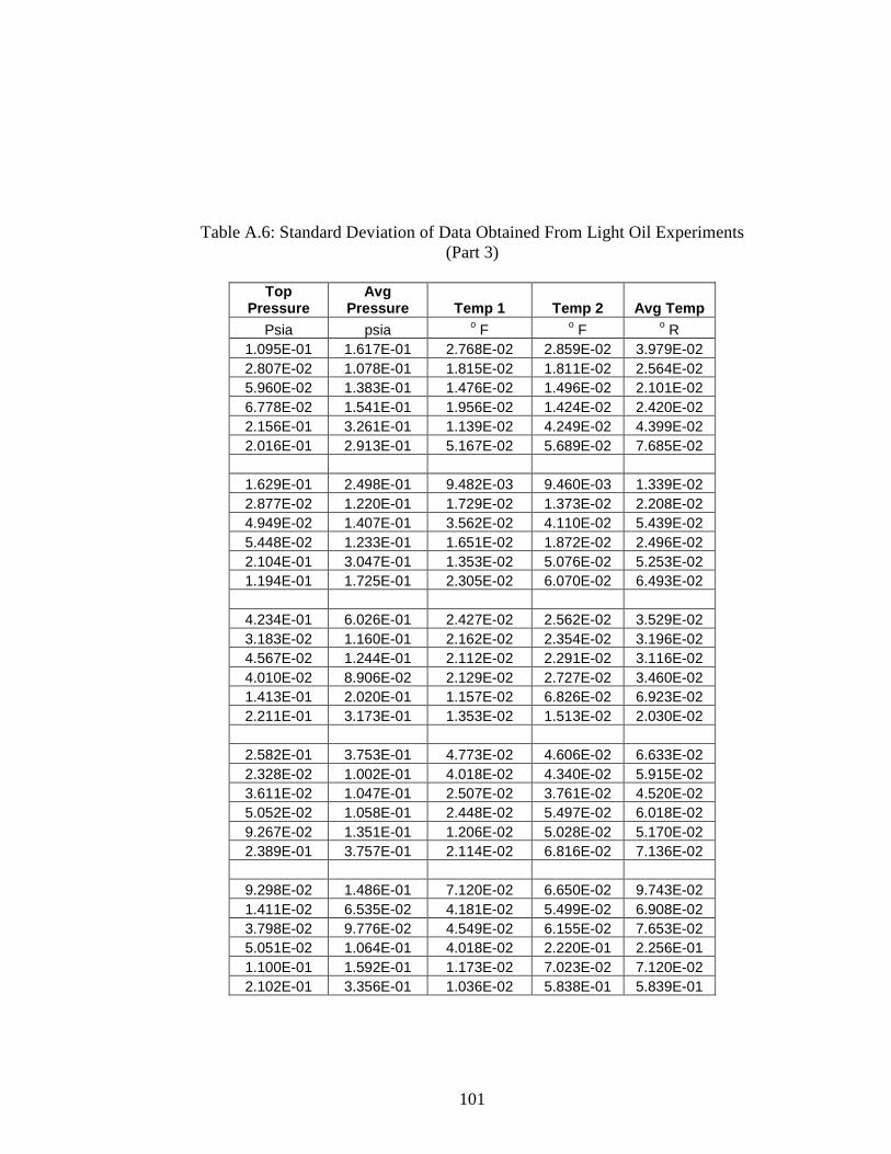
101
Table A.6: Standard Deviation of Data Obtained From Light Oil Experiments (Part 3)
Top
Pressure Avg
Pressure Temp 1 Temp 2 Avg Temp
Psia psia o F o F o R 1.095E-01 1.617E-01 2.768E-02 2.859E-02 3.979E-02 2.807E-02 1.078E-01 1.815E-02 1.811E-02 2.564E-02 5.960E-02 1.383E-01 1.476E-02 1.496E-02 2.101E-02 6.778E-02 1.541E-01 1.956E-02 1.424E-02 2.420E-02 2.156E-01 3.261E-01 1.139E-02 4.249E-02 4.399E-02 2.016E-01 2.913E-01 5.167E-02 5.689E-02 7.685E-02
1.629E-01 2.498E-01 9.482E-03 9.460E-03 1.339E-02 2.877E-02 1.220E-01 1.729E-02 1.373E-02 2.208E-02 4.949E-02 1.407E-01 3.562E-02 4.110E-02 5.439E-02 5.448E-02 1.233E-01 1.651E-02 1.872E-02 2.496E-02 2.104E-01 3.047E-01 1.353E-02 5.076E-02 5.253E-02 1.194E-01 1.725E-01 2.305E-02 6.070E-02 6.493E-02
4.234E-01 6.026E-01 2.427E-02 2.562E-02 3.529E-02 3.183E-02 1.160E-01 2.162E-02 2.354E-02 3.196E-02 4.567E-02 1.244E-01 2.112E-02 2.291E-02 3.116E-02 4.010E-02 8.906E-02 2.129E-02 2.727E-02 3.460E-02 1.413E-01 2.020E-01 1.157E-02 6.826E-02 6.923E-02 2.211E-01 3.173E-01 1.353E-02 1.513E-02 2.030E-02
2.582E-01 3.753E-01 4.773E-02 4.606E-02 6.633E-02 2.328E-02 1.002E-01 4.018E-02 4.340E-02 5.915E-02 3.611E-02 1.047E-01 2.507E-02 3.761E-02 4.520E-02 5.052E-02 1.058E-01 2.448E-02 5.497E-02 6.018E-02 9.267E-02 1.351E-01 1.206E-02 5.028E-02 5.170E-02 2.389E-01 3.757E-01 2.114E-02 6.816E-02 7.136E-02
9.298E-02 1.486E-01 7.120E-02 6.650E-02 9.743E-02 1.411E-02 6.535E-02 4.181E-02 5.499E-02 6.908E-02 3.798E-02 9.776E-02 4.549E-02 6.155E-02 7.653E-02 5.051E-02 1.064E-01 4.018E-02 2.220E-01 2.256E-01 1.100E-01 1.592E-01 1.173E-02 7.023E-02 7.120E-02 2.102E-01 3.356E-01 1.036E-02 5.838E-01 5.839E-01
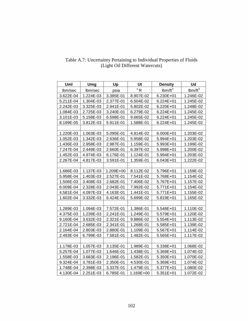
102
Table A.7: Uncertainty Pertaining to Individual Properties of Fluids (Light Oil Different Watercuts)
Uml Umg Up Ut Density Ud
lbm/sec lbm/sec psia o R lbm/ft3 lbm/ft3 3.622E-04 1.224E-03 3.385E-01 8.907E-02 6.230E+01 1.246E-02 5.211E-04 1.304E-03 2.377E-01 6.504E-02 6.224E+01 1.245E-02 2.242E-03 3.325E-03 2.941E-01 5.802E-02 6.220E+01 1.248E-02 1.084E-03 2.725E-03 3.240E-01 6.279E-02 6.224E+01 1.245E-02 3.101E-03 5.158E-03 6.598E-01 9.665E-02 6.224E+01 1.245E-02 8.199E-05 3.812E-03 5.911E-01 1.588E-01 6.224E+01 1.245E-02
1.220E-03 1.063E-03 5.095E-01 4.814E-02 6.000E+01 1.203E-02 1.052E-03 1.342E-03 2.636E-01 5.958E-02 5.994E+01 1.203E-02 1.436E-03 2.958E-03 2.987E-01 1.159E-01 5.993E+01 1.199E-02 7.247E-04 2.449E-03 2.660E-01 6.397E-02 5.998E+01 1.200E-02 1.452E-03 4.974E-03 6.176E-01 1.124E-01 5.994E+01 1.203E-02 2.267E-04 4.817E-03 3.591E-01 1.359E-01 6.043E+01 1.222E-02
1.686E-03 1.137E-03 1.209E+00 8.112E-02 5.796E+01 1.159E-02 5.958E-04 1.403E-03 2.527E-01 7.541E-02 5.768E+01 1.154E-02 1.506E-03 3.408E-03 2.682E-01 7.406E-02 5.767E+01 1.157E-02 6.009E-04 2.328E-03 2.043E-01 7.992E-02 5.771E+01 1.154E-02 4.581E-04 4.097E-03 4.163E-01 1.441E-01 5.771E+01 1.155E-02 1.602E-04 3.332E-03 6.424E-01 5.699E-02 5.819E+01 1.165E-02
1.289E-03 1.094E-03 7.572E-01 1.386E-01 5.548E+01 1.110E-02 4.375E-03 1.239E-03 2.241E-01 1.249E-01 5.579E+01 1.120E-02 9.160E-04 3.632E-03 2.321E-01 9.886E-02 5.554E+01 1.113E-02 2.721E-04 2.685E-03 2.341E-01 1.268E-01 5.585E+01 1.139E-02 2.164E-04 2.803E-03 2.880E-01 1.109E-01 5.567E+01 1.114E-02 2.493E-04 6.799E-03 7.581E-01 1.482E-01 5.565E+01 1.117E-02
1.178E-03 1.057E-03 3.135E-01 1.989E-01 5.338E+01 1.068E-02 5.257E-04 1.077E-03 1.646E-01 1.438E-01 5.369E+01 1.074E-02 1.558E-03 3.683E-03 2.196E-01 1.582E-01 5.350E+01 1.070E-02 9.324E-04 3.781E-03 2.350E-01 4.530E-01 5.369E+01 1.074E-02 1.748E-04 2.398E-03 3.337E-01 1.479E-01 5.377E+01 1.080E-02 4.130E-04 2.251E-03 6.785E-01 1.169E+00 5.351E+01 1.072E-02

103
Table A.8: Uncertainty of Superficial Liquid Velocity ( slv )
(Light Oil Different Watercuts)
Term 1 Term 2 1/area Total
Terms Uncertainty( vsl)
ft/sec 3.400E-11 6.129E-10 2.037E+01 2.543E-05 5.181E-04 7.052E-11 3.908E-10 2.037E+01 2.148E-05 4.375E-04 1.307E-09 2.228E-10 2.037E+01 3.911E-05 7.967E-04 3.051E-10 9.846E-11 2.037E+01 2.009E-05 4.093E-04 2.498E-09 2.411E-11 2.037E+01 5.022E-05 1.023E-03 1.746E-12 5.852E-12 2.037E+01 2.757E-06 5.616E-05
4.160E-10 6.119E-10 2.037E+01 3.206E-05 6.531E-04 3.097E-10 3.955E-10 2.037E+01 2.656E-05 5.410E-04 5.774E-10 2.233E-10 2.037E+01 2.830E-05 5.765E-04 1.469E-10 9.913E-11 2.037E+01 1.569E-05 3.195E-04 5.900E-10 2.526E-11 2.037E+01 2.481E-05 5.053E-04 1.416E-11 7.119E-12 2.037E+01 4.612E-06 9.396E-05
8.514E-10 6.072E-10 2.037E+01 3.819E-05 7.781E-04 1.073E-10 3.890E-10 2.037E+01 2.228E-05 4.539E-04 6.862E-10 2.214E-10 2.037E+01 3.013E-05 6.137E-04 1.090E-10 9.898E-11 2.037E+01 1.442E-05 2.938E-04 6.339E-11 2.516E-11 2.037E+01 9.410E-06 1.917E-04 7.630E-12 5.805E-12 2.037E+01 3.665E-06 7.467E-05
5.428E-10 6.090E-10 2.037E+01 3.394E-05 6.914E-04 6.185E-09 3.881E-10 2.037E+01 8.107E-05 1.652E-03 2.737E-10 2.197E-10 2.037E+01 2.221E-05 4.525E-04 2.388E-11 1.010E-10 2.037E+01 1.118E-05 2.277E-04 1.521E-11 2.410E-11 2.037E+01 6.270E-06 1.277E-04 2.018E-11 6.643E-12 2.037E+01 5.179E-06 1.055E-04
4.899E-10 6.167E-10 2.037E+01 3.326E-05 6.777E-04 9.645E-11 3.830E-10 2.037E+01 2.190E-05 4.461E-04 8.531E-10 2.169E-10 2.037E+01 3.271E-05 6.664E-04 3.035E-10 9.741E-11 2.037E+01 2.002E-05 4.079E-04 1.063E-11 2.450E-11 2.037E+01 5.927E-06 1.208E-04 5.994E-11 6.171E-12 2.037E+01 8.131E-06 1.656E-04

104
Table A.9: Uncertainty of Superficial Gas Velocity ( sgv )
(Light Oil Different Watercuts)
Term 1 Term 2 Term 3 1/area Total terms Uncertainty( vsg)
ft/sec 1.098E-04 1.568E-05 2.511E-09 2.037E+01 1.255E-04 2.282E-01 1.342E-04 1.639E-05 2.637E-09 2.037E+01 1.506E-04 2.500E-01 8.607E-04 5.051E-05 4.278E-09 2.037E+01 9.113E-04 6.150E-01 5.200E-04 1.172E-04 1.066E-08 2.037E+01 6.372E-04 5.143E-01 1.961E-03 2.161E-03 1.066E-07 2.037E+01 4.123E-03 1.308E+00 1.118E-03 2.547E-03 4.048E-07 2.037E+01 3.665E-03 1.233E+00
8.303E-05 3.517E-05 7.238E-10 2.037E+01 1.182E-04 2.215E-01 1.431E-04 2.052E-05 2.235E-09 2.037E+01 1.636E-04 2.606E-01 6.875E-04 5.145E-05 1.670E-08 2.037E+01 7.390E-04 5.538E-01 4.229E-04 8.128E-05 1.130E-08 2.037E+01 5.042E-04 4.574E-01 1.893E-03 1.214E-03 8.909E-08 2.037E+01 3.107E-03 1.135E+00 1.755E-03 5.118E-04 1.642E-07 2.037E+01 2.267E-03 9.699E-01
9.548E-05 1.088E-04 1.123E-09 2.037E+01 2.043E-04 2.912E-01 1.584E-04 1.636E-05 3.068E-09 2.037E+01 1.748E-04 2.693E-01 9.309E-04 3.605E-05 5.809E-09 2.037E+01 9.670E-04 6.335E-01 4.072E-04 3.661E-05 1.263E-08 2.037E+01 4.438E-04 4.292E-01 1.288E-03 4.429E-04 1.173E-07 2.037E+01 1.731E-03 8.475E-01 8.493E-04 9.077E-04 1.582E-08 2.037E+01 1.757E-03 8.539E-01
9.470E-05 2.488E-05 1.783E-09 2.037E+01 1.196E-04 2.228E-01 1.267E-04 8.765E-06 5.590E-09 2.037E+01 1.355E-04 2.371E-01 1.086E-03 1.962E-05 7.331E-09 2.037E+01 1.105E-03 6.773E-01 5.470E-04 4.581E-05 3.003E-08 2.037E+01 5.929E-04 4.960E-01 6.016E-04 1.583E-04 5.193E-08 2.037E+01 7.599E-04 5.616E-01 3.511E-03 1.223E-03 1.043E-07 2.037E+01 4.734E-03 1.402E+00
8.348E-05 1.688E-06 1.542E-09 2.037E+01 8.517E-05 1.880E-01 9.773E-05 2.878E-06 4.418E-09 2.037E+01 1.006E-04 2.043E-01 1.135E-03 1.458E-05 1.533E-08 2.037E+01 1.149E-03 6.906E-01 1.138E-03 2.945E-05 2.329E-07 2.037E+01 1.167E-03 6.961E-01 4.419E-04 1.109E-04 4.807E-08 2.037E+01 5.529E-04 4.790E-01 3.850E-04 6.540E-04 4.325E-06 2.037E+01 1.043E-03 6.580E-01
105
APPENDIX B
UNCERTAINTY ANALYSIS FOR HEAVY OIL DIFFERENT WATERC UTS (LL=6” BELOW INLET)

106
Table B.1: Data Obtained From Heavy Oil Experiments (Part 1)
watercut Oil Mass
Flow Rate
Oil Specific Gravity
Water Mass Flow Rate
Water Specific Gravity
Total Mass Flow Rate
% lbm/min ( - ) lbm/min ( - ) lbm/min 11.047 0.926 34.944 0.994 34.944
75.000 21.906 0.934 70.197 0.994 70.197 43.220 0.931 137.305 0.994 137.305 63.033 0.932 205.945 0.994 205.945 21.801 0.930 22.885 0.994 44.685
50.000 41.882 0.930 45.160 0.994 87.042 84.935 0.932 92.170 0.994 177.105 127.133 0.932 138.005 0.994 265.138 31.956 0.929 11.492 0.996 43.448
25.000 63.423 0.930 23.038 0.996 86.461 120.850 0.929 46.426 0.994 167.275 187.623 0.932 69.109 0.994 256.732 43.050 0.925 -0.657 0.994 43.050
0.000 83.110 0.908 -0.778 0.924 83.110 160.349 0.897 -0.773 0.924 160.349

107
Table B.2: Data Obtained From Heavy Oil Experiments (Part 2)
Total Mass Flow Rate
Total Specific Gravity
Mixture Density
Air Mass Flow Rate
Air Mass Flow Rate
Air Density
lbm/sec ( - ) lbm/ft3 lbm/min lbm/sec lbm/ft3 0.582 0.977 60.803 10.694 0.178 0.011 1.170 0.979 60.933 9.272 0.155 0.011 2.288 0.978 60.886 7.682 0.128 0.011 3.432 0.979 60.903 4.508 0.075 0.011
0.745 0.962 59.868 9.594 0.160 0.011 1.451 0.962 59.878 8.714 0.145 0.011 2.952 0.963 59.935 6.812 0.114 0.011 4.419 0.963 59.923 4.124 0.069 0.011
0.724 0.946 58.850 8.925 0.149 0.011 1.441 0.947 58.911 8.036 0.134 0.011 2.788 0.945 58.815 5.784 0.096 0.011 4.279 0.947 58.967 3.794 0.063 0.011
0.717 0.925 57.570 8.117 0.135 0.011 1.385 0.908 56.514 6.241 0.104 0.011 2.672 0.897 55.829 4.014 0.067 0.011

108
Table B.3: Data Obtained From Heavy Oil Experiments (Part 3)
Inlet Pressure
Top Pressure
Avg Pressure
Temp 1
Temp 2
Avg Temp
psia psia psia o F o F o R 32.560 32.123 32.341 84.243 86.155 545.199 30.915 30.502 30.709 85.404 89.280 547.342 30.065 29.365 29.715 87.732 92.264 549.998 30.000 29.388 29.694 91.633 91.775 551.704
30.075 29.713 29.894 84.134 87.074 545.604 30.045 29.709 29.877 85.286 89.312 547.299 30.019 29.483 29.751 87.474 92.564 550.019 30.005 29.466 29.736 92.177 92.510 552.343
29.455 29.097 29.276 81.635 90.621 546.128 30.015 29.623 29.819 78.771 86.638 542.704 29.786 29.233 29.510 87.267 92.002 549.634 30.004 29.550 29.777 92.206 93.243 552.724
29.911 29.566 29.739 84.597 91.793 548.195 27.552 27.254 27.403 95.818 99.811 557.814 30.334 29.987 30.160 92.441 97.372 554.907

109
Table B.4: Standard Deviation of Data Obtained From Heavy Oil Experiments (Part 1)
water cut
Oil Mass Flow Rate
Oil Specific Gravity
Water Mass Flow Rate
Water Specific Gravity
% lbm/sec ( - ) lbm/sec ( - ) 75 1.709E+00 3.189E-04 1.204E+00 3.087E-04
9.598E-01 6.667E-16 1.686E+00 5.004E-04 5.995E-01 1.523E-04 2.188E+00 4.192E-05 4.941E-01 6.505E-05 1.530E+00 4.000E-15
50 3.438E-01 4.493E-04 1.742E+00 1.822E-14 7.121E-01 3.030E-04 3.690E-01 1.211E-14 2.034E+00 6.263E-04 5.956E-01 3.264E-04 2.441E+00 4.994E-04 1.082E+00 1.023E-14
25 8.337E-01 5.931E-04 3.535E-01 1.444E-15 1.683E+00 1.311E-04 4.200E-01 1.111E-14 5.290E+00 6.725E-04 5.748E-01 6.338E-15 3.575E+00 3.234E-04 5.424E-01 1.334E-14
0 6.147E-01 1.920E-04 1.032E-01 4.449E-16 1.656E+00 7.221E-15 1.842E-01 1.178E-14 7.962E+00 9.722E-04 1.713E-01 1.544E-14

110
Table B.5: Standard Deviation of Data Obtained From Heavy Oil Experiments (Part 2)
Total Mass Flow Rate
Mixture Density
Air Mass Flow Rate
Air Density
Inlet Pressure
lbm/sec lbm/ft3 Lbm/sec lbm/ft3 psia 2.427E-02 4.438E-04 2.99E-03 6.835E-04 4.147E-01 2.205E-02 5.004E-04 2.29E-03 4.979E-04 3.390E-01 2.323E-02 1.580E-04 1.38E-03 6.315E-04 1.826E-01 1.687E-02 6.505E-05 7.09E-04 6.343E-04 1.873E-01
1.738E-02 4.493E-04 2.30E-03 6.350E-04 1.855E-01 9.009E-03 3.030E-04 2.04E-03 5.637E-04 2.191E-01 2.192E-02 7.063E-04 1.26E-03 5.972E-04 1.841E-01 2.936E-02 4.994E-04 6.97E-04 6.202E-04 2.056E-01
9.893E-03 5.931E-04 1.98E-03 4.965E-04 2.689E-01 1.752E-02 1.311E-04 1.73E-03 5.758E-04 1.491E-01 4.888E-02 6.725E-04 6.46E-03 4.568E-04 3.946E-01 3.431E-02 3.234E-04 5.89E-04 5.914E-04 1.663E-01
5.982E-03 8.666E-15 1.79E-03 4.606E-04 2.643E-01 1.534E-02 1.055E-14 1.06E-03 5.551E-04 8.934E-02 6.778E-02 1.889E-15 5.62E-04 5.397E-04 4.703E-01
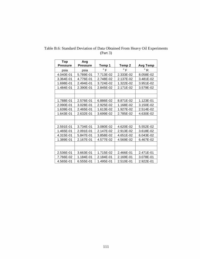
111
Table B.6: Standard Deviation of Data Obtained From Heavy Oil Experiments (Part 3)
Top
Pressure Avg
Pressure Temp 1 Temp 2 Avg Temp
psia psia o F o F o R 4.040E-01 5.789E-01 7.713E-02 2.333E-02 8.058E-02 3.364E-01 4.776E-01 2.748E-02 2.137E-02 3.481E-02 1.698E-01 2.494E-01 3.724E-02 1.322E-02 3.951E-02 1.484E-01 2.390E-01 2.845E-02 2.171E-02 3.579E-02
1.788E-01 2.576E-01 6.886E-02 8.871E-02 1.123E-01 2.090E-01 3.028E-01 2.925E-02 1.168E-02 3.150E-02 1.639E-01 2.465E-01 1.613E-02 1.927E-02 2.514E-02 1.643E-01 2.632E-01 3.699E-02 2.785E-02 4.630E-02
2.591E-01 3.734E-01 3.080E-02 4.620E-02 5.552E-02 1.465E-01 2.091E-01 2.147E-02 2.913E-02 3.618E-02 4.315E-01 5.847E-01 3.858E-02 4.651E-02 6.043E-02 1.389E-01 2.167E-01 4.577E-02 4.569E-02 6.467E-02
2.536E-01 3.663E-01 1.715E-02 2.466E-01 2.471E-01 7.766E-02 1.184E-01 2.184E-01 2.169E-01 3.078E-01 4.565E-01 6.555E-01 1.495E-01 2.510E-01 2.922E-01
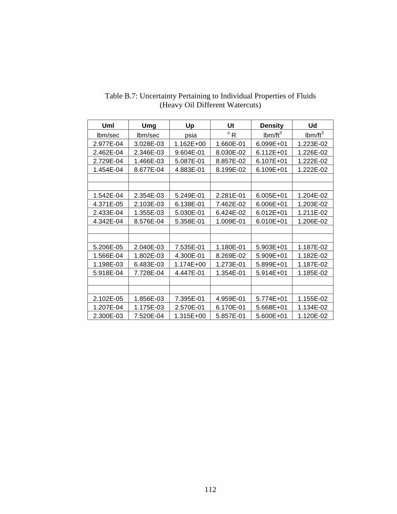
112
Table B.7: Uncertainty Pertaining to Individual Properties of Fluids (Heavy Oil Different Watercuts)
Uml Umg Up Ut Density Ud
lbm/sec lbm/sec psia o R lbm/ft3 lbm/ft3 2.977E-04 3.028E-03 1.162E+00 1.660E-01 6.099E+01 1.223E-02 2.462E-04 2.346E-03 9.604E-01 8.030E-02 6.112E+01 1.226E-02 2.729E-04 1.466E-03 5.087E-01 8.857E-02 6.107E+01 1.222E-02 1.454E-04 8.677E-04 4.883E-01 8.199E-02 6.109E+01 1.222E-02
1.542E-04 2.354E-03 5.249E-01 2.281E-01 6.005E+01 1.204E-02 4.371E-05 2.103E-03 6.138E-01 7.462E-02 6.006E+01 1.203E-02 2.433E-04 1.355E-03 5.030E-01 6.424E-02 6.012E+01 1.211E-02 4.342E-04 8.576E-04 5.358E-01 1.009E-01 6.010E+01 1.206E-02
5.206E-05 2.040E-03 7.535E-01 1.180E-01 5.903E+01 1.187E-02 1.566E-04 1.802E-03 4.300E-01 8.269E-02 5.909E+01 1.182E-02 1.198E-03 6.483E-03 1.174E+00 1.273E-01 5.899E+01 1.187E-02 5.918E-04 7.728E-04 4.447E-01 1.354E-01 5.914E+01 1.185E-02
2.102E-05 1.856E-03 7.395E-01 4.959E-01 5.774E+01 1.155E-02 1.207E-04 1.175E-03 2.570E-01 6.170E-01 5.668E+01 1.134E-02 2.300E-03 7.520E-04 1.315E+00 5.857E-01 5.600E+01 1.120E-02

113
Table B.8: Uncertainty Analysis of Superficial Liquid Velocity ( slv )
(Heavy Oil Different Watercuts)
Term 1 Term 2 1/area Total terms Uncertainty( vsl)
ft/sec 2.398E-11 3.712E-12 2.037E+01 5.262E-06 1.072E-04 1.632E-11 1.494E-11 2.037E+01 5.591E-06 1.139E-04 2.009E-11 5.689E-11 2.037E+01 8.774E-06 1.787E-04 5.704E-12 1.278E-10 2.037E+01 1.156E-05 2.354E-04
6.632E-12 6.262E-12 2.037E+01 3.591E-06 7.315E-05 5.328E-13 2.368E-11 2.037E+01 4.921E-06 1.002E-04 1.648E-11 9.895E-11 2.037E+01 1.074E-05 2.189E-04 5.251E-11 2.204E-10 2.037E+01 1.652E-05 3.365E-04
7.826E-13 6.154E-12 2.037E+01 2.634E-06 5.366E-05 7.068E-12 2.409E-11 2.037E+01 5.582E-06 1.137E-04 4.146E-10 9.160E-11 2.037E+01 2.250E-05 4.583E-04 1.007E-10 2.125E-10 2.037E+01 1.770E-05 3.606E-04
1.333E-13 6.251E-12 2.037E+01 2.527E-06 5.147E-05 4.564E-12 2.418E-11 2.037E+01 5.361E-06 1.092E-04 1.697E-09 9.221E-11 2.037E+01 4.230E-05 8.618E-04
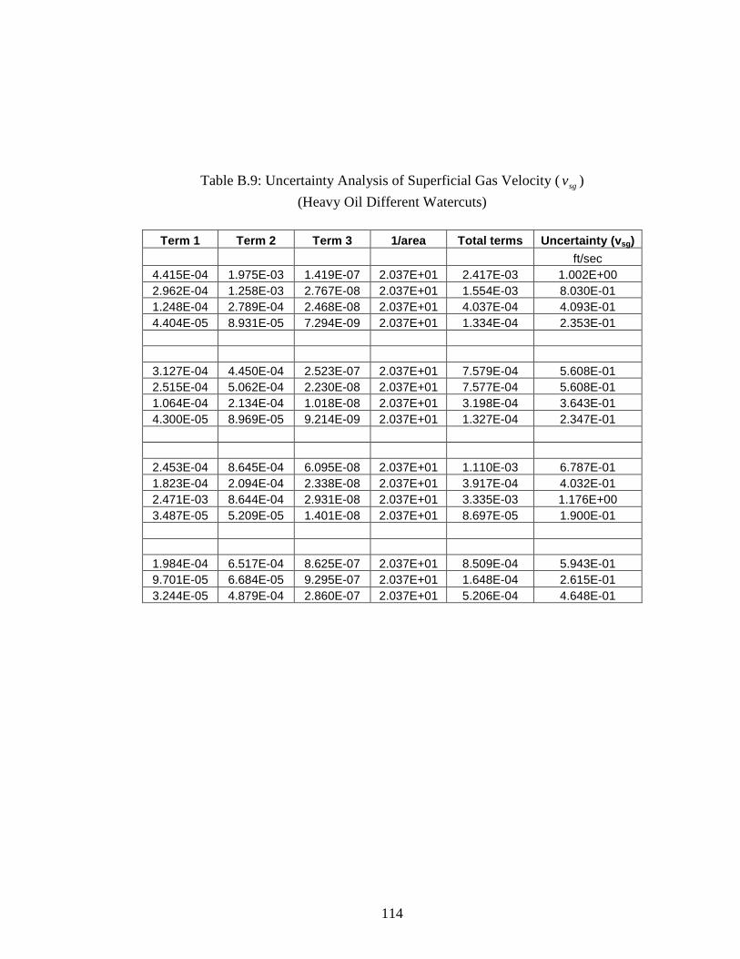
114
Table B.9: Uncertainty Analysis of Superficial Gas Velocity ( sgv )
(Heavy Oil Different Watercuts)
Term 1 Term 2 Term 3 1/area Total terms Uncertainty (vsg)
ft/sec 4.415E-04 1.975E-03 1.419E-07 2.037E+01 2.417E-03 1.002E+00 2.962E-04 1.258E-03 2.767E-08 2.037E+01 1.554E-03 8.030E-01 1.248E-04 2.789E-04 2.468E-08 2.037E+01 4.037E-04 4.093E-01 4.404E-05 8.931E-05 7.294E-09 2.037E+01 1.334E-04 2.353E-01
3.127E-04 4.450E-04 2.523E-07 2.037E+01 7.579E-04 5.608E-01 2.515E-04 5.062E-04 2.230E-08 2.037E+01 7.577E-04 5.608E-01 1.064E-04 2.134E-04 1.018E-08 2.037E+01 3.198E-04 3.643E-01 4.300E-05 8.969E-05 9.214E-09 2.037E+01 1.327E-04 2.347E-01
2.453E-04 8.645E-04 6.095E-08 2.037E+01 1.110E-03 6.787E-01 1.823E-04 2.094E-04 2.338E-08 2.037E+01 3.917E-04 4.032E-01 2.471E-03 8.644E-04 2.931E-08 2.037E+01 3.335E-03 1.176E+00 3.487E-05 5.209E-05 1.401E-08 2.037E+01 8.697E-05 1.900E-01
1.984E-04 6.517E-04 8.625E-07 2.037E+01 8.509E-04 5.943E-01 9.701E-05 6.684E-05 9.295E-07 2.037E+01 1.648E-04 2.615E-01 3.244E-05 4.879E-04 2.860E-07 2.037E+01 5.206E-04 4.648E-01