Liquidity Constraint Tightness and ConsumerResponses to Fiscal Stimulus Policy∗

Claus Thustrup KreinerUniversity of Copenhagen and CEPR

David Dreyer LassenUniversity of Copenhagen

Søren Leth-PetersenUniversity of Copenhagen

August 2014

Abstract

Consumption theory posits that variation in marginal interest rates across con-sumers predicts spending responses to stimulus policies. We test this directly us-ing administrative records with account level information about loans and depositsto measure the response to a Danish stimulus policy transforming illiquid pensionwealth into liquid wealth. The data reveal substantial variation in marginal interestrates across consumers, and this predicts spending responses. Differences in interestrates across consumers cannot be explained by short-lived shocks appearing withinthe duration of a typical business cycle but is consistent with persistent heterogene-ity, for example in the degree of impatience.

∗We thank Sumit Agarwal, Martin Browning, Chris Carroll, Wojciech Kopczuk, Jonathan Parker,Emmanuel Saez, Matthew Shapiro, Joel Slemrod, conference participants at the AEA 2014 meetings, theCEPR Public Policy symposium, and the NBER Summer Institute, and numerous seminar participantsat Columbia, Copenhagen, LSE/UCL, Lund, Michigan, Uppsala and Aarhus for constructive commentsand discussions. Amalie Sofie Jensen, Katarina Helena Jensen, Anders Priergaard Nielsen, Rasmus AarupPoulsen and Gregers Nytoft Rasmussen provided excellent research assistance. We are grateful to theDanish tax administration (SKAT) for providing data on loans and deposits and to ATP for providingdata on pension accounts. Financial support from The Danish Council for Independent Research (SocialScience) and from the Economic Policy Research Network (EPRN) is gratefully acknowledged. Contactinfo: ctk@econ.ku.dk, ddl@econ.ku.dk, soren.leth-petersen@econ.ku.dk.

1 Introduction

Across the world, governments reacted to the large negative shock that hit the global

economy in 2008 by adopting unprecedented fiscal stimulus policies, in many cases with

the explicit aim of increasing household consumption to boost aggregate spending. Many

empirical studies have documented that consumers do raise spending in response to stim-

ulus policy, including recent studies by Shapiro and Slemrod (2009), Sahm, Shapiro, and

Slemrod (2010), Parker et al. (2013), Broda and Parker (2014), and Agarwal and Qian

(2014), and find spending propensities in the range 0.3-0.9.

These results are in contrast to the prediction of the Permanent Income Hypothe-

sis/canonical Life-Cycle model with perfect capital markets where tax rebates just raise

household savings, without having any stimulus effect on the economy. A standard ex-

planation for this prediction failure of the basic Permanent Income Hypothesis is the

prevalence of liquidity constraints (Zeldes, 1989). If some households are constrained by

lack of access to liquidity then stimulus policy reduces the tightness of the constraints and

boosts the spending of these households. In this paper we employ a unique data set with

information about all household borrowing and saving at the account level to provide a

direct test of the importance of liquidity constraint tightness, and proceed to investigate

why liquidity constraint tightness varies across consumers.

Liquidity constraints are difficult to identify empirically and previous studies of con-

sumer responses to stimulus policy have used different types of proxies such as low house-

hold income, young persons and low liquid asset holdings to classify households as liquidity

constrained (Shapiro and Slemrod, 2003, 2009; Sahm, Shapiro, and Slemrod, 2010; Soule-

les, 1999; Johnson et al., 2006; Parker et al., 2013; Broda and Parker, 2014). However,

a challenge for these studies is that differences in access to liquidity is one of degree and

not of kind in that the tightness of liquidity constraints is a continuous variable reflecting

how costly additional liquidity is to the consumer and it is this shadow value of liquidity

that theoretically determines the propensity to consume (Browning and Lusardi, 1996).

For example, one consumer may have collateral and borrow at a low interest rate, while

1

another may have used up his collateral-backed line of credit and therefore pays a higher

interest on the last dollar borrowed. We demonstrate in a basic consumption model how

variation across consumers in the marginal interest rate observed prior to the stimulus

policy, measuring liquidity constraint tightness, predicts variation in spending responses

to stimulus policy.

We test this liquidity constraint hypothesis directly using a novel Danish data set con-

taining third-party reported administrative records of all individual-level loan and deposit

accounts that enables us to compute pre-reform consumer level marginal interest rates.

The data reveal substantial variation in the marginal interest rates paid by consumers,

varying from close to 0 to more than 20 percent across people in our sample in 2008. We

employ this data in an analysis of a Danish fiscal stimulus policy that allowed consumers

to take out wealth from otherwise inaccessible pension accounts within a seven month

window during 2009, thereby transforming illiquid pension wealth into liquid wealth avail-

able for spending. The policy changed the timing of access to wealth without affecting

the level of wealth, making it ideal for testing the importance of liquidity constraints for

spending responses to stimuli.

We measure the spending effect of the reform through a survey conducted in January

2010, immediately after the pay-out window had closed, resulting in about 5,000 completed

interviews with information about spending behavior related to the pension payout. Our

survey method follows previous studies (e.g., Shapiro and Slemrod, 2003, and Parker et al.,

2013) and asks respondents directly about the change in their total spending, net saving

and pension saving in 2009 due to the stimulus payment.

We match the survey data at the person level to the loan and deposit accounts data

as well as to income tax records and other administrative registers containing information

about demographics, incomes and wealth, and broad categories of financial asset holdings

for the period 1998-2009. By comparing answers from the survey about the allocation

of the payout on spending, net savings, and pension savings to corresponding measures

constructed from the register data over several years surrounding the time of the stimulus

2

reform, we show that respondents understand the counterfactual nature of the survey

question.

We find that the variation in marginal interest rates across consumers, observed prior

to the stimulus reform, is strongly significant in predicting the variation in spending re-

sponses, with a 1 percentage point difference in the interest rate between consumers being

associated with a 0.5 percentage point difference in the propensity to spend. These find-

ings are in line with the theory and suggest that liquidity constraints are important for

explaining spending responses to stimulus policies, even if other factors, e.g. size effects,

also turn out to be important for explaining the total response to the stimulus policy.

The substantial variation across consumers in pre-reform marginal interest rates, and

therefore also in spending responses to the stimulus reform, may be due to idiosyncratic,

temporary income shocks occurring in the downturn before the reform, or it may be

due to persistent heterogeneity in the demand for liquidity, for example because of fixed

differences in how consumers discount future consumption. We show that the marginal

interest rate is strongly correlated with the ratio of liquid assets to income more than a

decade earlier. This result indicates that differences in liquidity constraint tightness across

consumers, observed just before the stimulus policy implementation, reflect heterogeneity

across consumers that is permanent or persistent to a degree that cannot be accounted for

by shocks appearing within the horizon of a typical business cycle.

Our results contribute in different ways to the literature measuring the effects of stimu-

lus policies and the role of liquidity constraints. It is the first study that directly examines

the role of variation in the cost of liquidity across consumers for the propensity to spend

out of a stimulus. Johnson et al. (2006) estimate the change in consumption expenditures

caused by the 2001 federal income tax rebates. They show that people with little liquid

wealth are likely to spend more and point to liquidity constraints as a likely driver of

spending responses. Souleles (1999) examines the effects of tax refunds and reach similar

findings. We show that proxying liquidity constraints by the ratio of liquid assets to in-

come does not capture the full underlying heterogeneity in liquidity constraint tightness,

3

thereby underestimating its role in explaining consumption responses to stimulus policy.

Agarwal et al. (2007) show, using credit card data, that consumers initially increased

credit card payments but soon after increased spending following the 2001 US income tax

rebate. Similarly, Agarwal and Qian (2014) use credit and debit card data and find that

those with low bank balances and credit card limits respond more strongly to a Singa-

porean stimulus policy. The focus on credit card use is interesting because credit cards

are likely to be the source of credit that carries the highest marginal cost of liquidity. The

high frequency of the credit card data makes it possible to follow the short term dynamics

of spending, but the Agarwal et al. and Agarwal and Qian studies do not have data on

other household assets and spending and does not measure the cost of liquidity directly.

Parker et al. (2013) investigate the effect of the 2008 tax rebate using the US consumer

expenditure survey (CEX) and find that low income households tend to have a higher

propensity to spend, but do not provide clear evidence for the importance of liquidity

constraints. Broda and Parker (2014), also measuring the effect of the 2008 tax rebate

but using a larger data set based on scanner data, find that low liquid wealth households

account for the majority of the spending response, but find no clear difference between low

and high income households. There is, in fact, little consensus about the role of liquidity

constraints for the propensity to spend out of stimuli. Shapiro and Slemrod (2003, 2009)

and Sahm, Shapiro, and Slemrod (2010) examine the effects of the 2001 and 2008 tax

rebates using survey information and find that respondents with low income do not have

a higher propensity to spend the stimulus. To the extent that income is an indicator of

being affected by constraints, these results could be interpreted to mean that constraints

are not important.

Our results potentially reconcile the disparate findings about the importance of liquid-

ity constraints. Common to all these studies is that they do not have a precise measure

of how binding liquidity constraints are. We find that the pre-reform marginal interest

rates of consumers predict the spending responses to stimulus policy, also after controlling

for various income measures, financial assets, expectations, size of the payout, age and

4

other demographic characteristics. The marginal interest rate is correlated with the level

of liquid assets but only weakly correlated with income. This may explain why studies

using low income as an indicator for being liquidity constrained find that it is unimportant

for consumption responses, while studies using low levels of liquid assets as an indicator

find that liquidity constraints play an important role in explaining consumer behavior.

The finding of substantial heterogeneity in pre-reform marginal interest rates is also

consistent with results from a broader literature about the role of liquidity constraints and

consumption behavior, including Gross and Souleles (2002) and Leth-Petersen (2010),

showing that changes in the supply of credit have an effect on consumption for some, but

not all, groups of consumers.

None of the aforementioned studies analyze why some individuals are liquidity con-

strained while others are not. Our results point to permanent, or very persistent, het-

erogeneity across consumers that generate variation in liquidity constraint tightness and,

therefore, also in spending responses to stimulus policy. While not identifying any partic-

ular model, such a pattern is consistent with theory of savings behavior where consumers

are heterogeneous with respect to how they discount the future, including Mankiw’s (2000)

spenders-savers model of fiscal policy as well as recent empirical work by Alan and Brown-

ing (2010) that rejects homogeneity of discount factors, Hurst (2006) that presents empir-

ical evidence consistent with the view that some agents discount the future heavily while

others do not, and Carroll et al. (2013) that introduces a fixed idiosyncratic time pref-

erence factor into a buffer-stock model and is able to explain the US wealth distribution

and the magnitude of responses to stimulus policies.

The next section presents details of the Danish fiscal stimulus reform. Section 3 shows

why liquidity constraint tightness may vary across households and how this leads to hetero-

geneity in consumption responses. The following sections introduce the data and present

the results. The final section concludes.

5

2 The Danish fiscal stimulus policy

On March 1, 2009, the centre-right Danish government announced a major fiscal stimulus

policy initiative, aimed at stabilizing the Danish economy in the midst of the financial

and economic crisis: The Special Pension (SP) payout. The SP scheme was introduced

in 1998 as a compulsory individual pension account, into which everyone earning income

in Denmark deposited one percent of their gross earnings. The scheme was administered

by the largest Danish public pension fund ATP, everyone earned the same rate of interest

on funds in the scheme, and individuals would receive their pension at age 65. Payments

into the scheme were suspended in 2004 and from here no more money were paid in to

the accounts. The stimulus policy gave individuals the possibility of having the balance

on their SP-account paid out in the period from June 1 to December 31 in 2009, and

the payout was to be taxed at 35 percent for the first 15,000 DKK (approx. 3,000 USD)

and at 50 percent beyond 15,000 DKK, reflecting that all pension benefits are taxable in

Denmark.

The stimulus policy was noteworthy for several reasons: First, by allowing individuals

to withdraw a part of their own pension funds that would otherwise be unattainable

until age 65, the stimulus payment received by an individual would be financed by a

corresponding reduction in the person’s pension wealth rather than government borrowing

and future tax increases. The stimulus policy therefore preserved Ricardian equivalence

at the individual level: Having the money paid out and used for present spending would

restrict future spending possibilities with certainty.1

Second, the stimulus policy initiative was unanticipated. This can be seen from Figure

1, which shows the number of mentions of the words “SP” and “pension” in all Danish

media, electronic and print, from October 2008 to June 2009. The early spikes are due

to reports that the government first proposed and then abandoned plans to reinstate

payments into the SP as part of the 2009 government budget proposal, and the small

1The tax scheme involved a small wealth effect for high wage earners who could obtain a higher netwealth from taking the SP funds out and placing the funds in a private pension scheme if the rate ofreturns are expected to be the same on the two schemes.

6

blip in early February was media reports on capital losses on accumulated SP-savings

following the financial crisis, after which there was no mention of the SP until March

1, 2009. Because the policy was unanticipated, variation in pre-reform marginal interest

rates across consumers is unrelated to the reform.

Third, the policy was transparent. All account holders received a personal letter, shown

in Figure A1 in the appendix, from ATP with a pre-filled form including the account

balance on May 1, 2009. To have the balance paid out, account holders should sign a slip

and return it in an enclosed, stamped envelope. The money would then be transferred

directly to the holder’s main bank account, already on file.

Fourth, the stimulus was large. On June 1, 2009, there were 2,603,565 individuals with

an SP account, corresponding to 70 percent of the adult population (≥ 25 years), and

the average account balance was 14,924 DKK (approximately 3,000 USD). Of the account

holders, 94 percent chose to have their funds paid out. The average gross payout was 15,447

DKK and the corresponding average payout net of taxes was 9,536 DKK (approximately

1,900 USD). In comparison, the 2008 US tax rebates were between $300 and $600 per

adult and $300 per dependent child (Parker et al., 2013). The total sum paid out was 23.3

billion DKK net of taxes, equal to 1.4 percent of GDP.

< Figure 1 >

3 A simple theory of liquidity constraint tightness

and consumer responses to stimulus policy

This section illustrates within a basic two-period model why consumers may face different

marginal interest rates prior to a stimulus reform and how this variation in liquidity

constraint tightness generates differences in spending responses to a stimulus policy.

Let c1 and c2 denote the consumption levels of a household in period 1 and period 2,

respectively, and assume that consumer behavior is governed by a standard homothetic

utility function u (c1, c2).2 The consumer has both illiquid wealth and liquid wealth (which

2Within the class of homothetic utility functions is the specification u (c1, c2) = c1−θ1 / (1− θ) +

7

may be negative) at the beginning of period 1. Let y1 denote the cash-on-hand in period 1

such as earnings and liquid wealth carried over from the previous period, and let a1 denote

illiquid consumer wealth which is not accessible before period 2, e.g. a positive balance on

pension accounts that cannot be withdrawn or used as collateral for loans. The consumer

budget constraint in period 1 then becomes

c1 ≤ y1 + d, (1)

where d is consumer debt at the end of period 1 (or savings if d < 0). The consumption

level in the second period has to fulfill

c2 ≤ y2 + (1 + r̃) a1 − (1 + r̄) d, (2)

where y2 is earnings and other non-capital income in period two, r̃ is a fixed rate of return

on illiquid wealth, and r̄ is the average interest rate on consumer debt/savings. We assume

that the interest rate on a new loan of the consumer r (d) is (weakly) increasing in the

existing level of consumer debt d, reflecting a higher risk of default and a lower level of

collateral at higher debt levels. This is illustrated by the black piecewise linear budget

line in Panel A of Figure 2, showing that the intertemporal consumption trade-off faced

by the consumer increases as he raises his consumption level in period 1. We assume for

simplicity that the rate of return on savings is constant and equal to r̃ such that r (d) = r̃

for d < 0. The average interest rate on consumer debt/savings in eq. (2) is then equal to

r̄ =

{ (´ d0r (h) dh

)/d d ≥ 0

r̃ d < 0. (3)

The consumer’s optimum, illustrated in Panel B of Figure 2 for different types of prefer-

ences by the points X, Y and Z, is characterized by a standard tangency condition derived

from eqs (1)-(3):

MRS (c1/c2) ≡u1 (c1, c2)

u2 (c1, c2)= 1 + r (d) , (4)

βc1−θ2 / (1− θ) commonly used in consumption theory and macro economics and where β is the sub-

jective discount factor while θ > 0 is the coefficient of relative risk aversion. Note that since our focus ison predicting consumer behavior, this utility function may be different from the utility metric determiningthe well-being of the consumer due to present bias or other types of behavioral effects, without affectingthe results.

8

where the interest rate on marginal lending r (d) depends on the consumption choice

(through d), and where the marginal rate of substitution is a function only of relative

consumption levels c2/c1 because of the assumption of homothetic preferences. Note that

the optimum condition (4) may be rewritten as

MRS (c1/c2) = (1 + r̃) (1 + ψ) , ψ (d) ≡ r (d)− r̃1 + r̃

,

where ψ is the shadow price of liquidity (Browning and Lusardi, 1996). This shows that

a high marginal interest rate of the consumer, r (d), is equivalent to a high shadow price

of liquidity, i.e. a tight liquidity constraint.

Now consider a fiscal stimulus policy that allows the consumer to transfer a certain

amount of illiquid wealth a1 to cash-on-hand wealth y1. We assume that the permitted

transfer amount is small compared to total wealth allowing us to approximate the effect

of the reform as a marginal change dx giving the consumer the opportunity to change the

allocation of wealth between liquid and illiquid wealth according to

dy1 = −da1 = dx. (5)

By differentiating equations (1)–(4) wrt. x and using the relationship (5), we obtain:

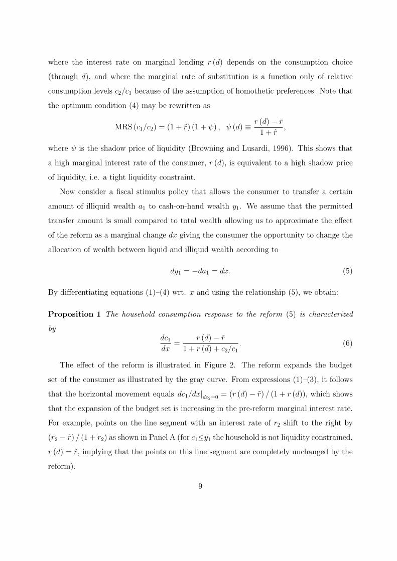
Proposition 1 The household consumption response to the reform (5) is characterized

bydc1dx

=r (d)− r̃

1 + r (d) + c2/c1. (6)

The effect of the reform is illustrated in Figure 2. The reform expands the budget

set of the consumer as illustrated by the gray curve. From expressions (1)–(3), it follows

that the horizontal movement equals dc1/dx|dc2=0 = (r (d)− r̃) / (1 + r (d)), which shows

that the expansion of the budget set is increasing in the pre-reform marginal interest rate.

For example, points on the line segment with an interest rate of r2 shift to the right by

(r2 − r̃) / (1 + r2) as shown in Panel A (for c1≤y1 the household is not liquidity constrained,

r (d) = r̃, implying that the points on this line segment are completely unchanged by the

reform).

9

Panel B shows the consumption response to a stimulus policy for different types of

consumer preferences. Consider first a person with indifference curves represented by I1

and I2, where the optimum before the reform is point Y. With homothetic preferences,

MRS is constant along a ray from the origin, implying that the new optimum is at Y’.

A more impatient person will be at Z, with a higher marginal interest rate before the

reform, and move to Z’, which gives a larger immediate consumption response to the

stimulus policy. On the other hand, a person at point X where r (d) = r̃ will not respond

to the reform at all. This shows that variation in preferences across consumers create

variation in consumer marginal interest rates before the stimulus reform and that this

variation in liquidity constraint tightness is related to consumption responses, with larger

responses for consumers with high pre-reform marginal interest rates.3

< Figure 2 >

Differences across consumers in pre-reform marginal interest rates may also arise be-

cause of heterogeneity in the budget set. For example, one consumer may receive the main

part of life time income in period 1 and save funds for period 2 consumption, while another

consumer may receive the main part of life time income in period 2 and borrow money

in period 1. This is illustrated in Figure 3 where household A has all life time income in

period 1 while household B has a large part of life time income in period 2 implying that

household A faces the intertemporal trade-off 1+ r̃ everywhere, while the trade-off is larger

for household B when borrowing money. With identical preferences and no credit market

imperfections both households would attain the consumption levels at X but because B

faces a higher marginal interest, she obtains only the consumption level at Y in Figure

3. The stimulus policy does not have any impact on the budget set of household A but

expands the budget set of household B and moves the optimum from Y to Y’, thereby

increasing current consumption. In this case, we therefore also get a positive relationship

3We have assumed that the initial consumer optimum is not at a kink. At a kink, we have dc1/dx = 1.If all individuals with positive consumption responses to the stimulus policy were initially at kinks thenthere would not be any relationship between consumption responses and pre-reform interest rates incontrast to the empirical evidence.

10

across households between liquidity constraint tightness and consumption responses to the

stimulus policy.

< Figure 3 >

Our data reveals substantial variation in observed marginal interest rates across con-

sumers. Two leading explanations for this variation are differences in preferences (patience

and risk aversion) and differences in timing of income (Deaton, 1999). In both cases, the

basic theory predicts that the observed pre-reform variation in marginal interest rates,

and therefore in liquidity constraint tightness, across consumers is positively related to

the differences in consumption responses to fiscal stimulus policy.

4 Data

The measurement of consumer spending responses to the stimulus policy is based on survey

data collected in January 2010 for a random sample of persons with SP-savings. For that

purpose, we commissioned a survey company that asked individuals about their response to

the SP-release. The survey data are joined at the individual level with third-party reported

administrative register data from the Danish Tax Authorities containing information about

loans, deposits and interest payments, used to compute marginal interest rates, as well as

a host of background information from other administrative registers.

4.1 Survey data and the spending response to the stimulus pol-icy

The window of the SP-release ended 31 December 2009. Shortly thereafter, in weeks 4-7

2010, we issued a telephone administered survey where we asked about the use of the

SP-funds. Each interview lasted 10-12 minutes and covered 40 questions about the SP-

policy and a range of other topics. The questions about the SP-policy were placed in the

beginning of the interview and were followed by questions about the respondents’ financial

situation and expectations regarding the future. In the survey we asked respondents about

11

their SP-account balance, whether the money was withdrawn and finally the following

question:4

The sum of money that you have at your disposal is the sum of money that

you have available for spending, saving, and reducing your debt. The SP pay-

out increased the amount that you have at your disposal in 2009. Considering

this increase, how did you allocate it:

- to increase spending (for example on food, traveling, clothes, televisions,

cars, home appliances, computers, restaurants, maintaining the house, or other

types of spending);

- to increase your free savings (i.e. putting money in the bank, buying

shares, bonds, or other securities);

- to reduce your debt;

- to increase your pension savings?

Respondents were sampled randomly from the entire set of SP-account holders. The

response rate in the survey is 50 percent when including item-nonresponses among non-

respondents, resulting in 5,055 completed interviews.5 We know the identity of non-

respondents and we are therefore able to characterize differences between respondents and

nonrespondents in terms of the variables available in the population-wide administrative

registers. In Appendix Table A1 we show that nonrespondents are on average slightly

younger, slightly more likely to be single, renters, have lower income, and smaller SP-

accounts. These differences are statistically significant but quantitatively small.6 Based

on the 2008 characteristics observed in the administrative registers, we have estimated the

4The question is inspired by Shapiro and Slemrod (1995, 2003). In section 5.1 we validate the surveyanswers against register data.

5Two data sources that have been used extensively for measuring the effect of stimulus policies inthe US are the CEX and the Michigan Survey of Consumers. The response rate in the CEX is 70-75% (http://www.bls.gov/cex/2012/csxintvw.pdf) and it is 40% in the Michigan Survey of Consumers(personal communication with the staff).

6The fact that we have more owners among respondents could suggest that we have more wealthyhand-to-mouth consumers, cf. Kaplan and Violante (2014), with high spendings rates. However, we notethat the differences are small, and that participants do not have less fiancial assets suggesting that theyare not likely to be more prone to behave as if liquidity constrained.

12

propensity to participate in the survey and recalculated our estimates weighting with the

inverse of the probability that the observation is included. If the particpation decision is

adequately captured by these charcteristics used for estimating the propensity score then

this would give a consistent estimate of the effect in the population. The results from this

exercise (not reported) did not deviate in any important way from the results presented

in the paper.

The survey question allows respondents to distribute the stimulus across all alterna-

tives. We use this information to calculate a marginal propensity to spend by putting the

amount spent in proportion to the total pay-out. Figure 4 shows a scatter plot of the

propensity to spend against the size of the SP payout together with a local polynomial

regression through the data. Most of the responses are corner solutions, either spend

(63%) or not spend (33%). The smoothed regression shows that the propensity to spend

is higher among respondents with small SP-accounts balances.

< Figure 4 >

4.2 Third party reported register data and computation of house-hold interest rates

The register data are of three types, covering different periods and providing different

amounts of detail. First, we have the register with information about SP-accounts from

the government pension fund, ATP. The data includes information about all SP-accounts

and the value of these on 1 May 2009. These data were used to draw the random sample

of persons that were interviewed.

The second type of register data includes standard demographic information from sev-

eral public administrative registers as well as information from the income-tax register for

the period 1998-2009. The income tax register holds detailed information about incomes

and values of assets and liabilities measured at the last day of the year. The asset and

liability information that we have access to from these registers is aggregated into broad

classes such as bonds, stocks, cash in banks, mortgage loans and the sum of other loans.

13

An important feature of these data is that they are organized longitudinally, enabling us

to track incomes and assets/liabilities back in time for the persons in our survey. Another

attractive feature is that the data are third party reported: Information about earnings is

collected directly from employers and information about transfer income from government

institutions, while information about the value of assets and liabilities by the end of the

year is reported directly from banks and other financial institutions. The tax authorities

use the income information to calculate tax liabilities and the wealth data to cross check

if reported income is consistent with the level of asset accumulation from one year to the

next. A recent study by Kleven et al. (2011) conducted a large scale randomized tax

auditing experiment in collaboration with the Danish tax authorities and documents that

tax evasion in Denmark is very limited, in particular among wage earners. This indicates

that the third party reported information about income collected by the tax authorities is

of very high quality; see also Chetty et al. (2011) for more detailed information on Danish

income-tax data, and Leth-Petersen (2010) for a detailed description of the wealth data.

The third type of register data is obtained from the raw data files of the tax authorities

and provide information about every individual deposit and loan account held by the

persons included in our sample in 2007 and 2008. These data provide information about

the value of deposits and loans at individual account levels at the last day of the year

as well as interest payments over the past year.7 We use the information from these files

to calculate the realized marginal interest rate before the reform for each person in our

survey.

To do this we link the interview persons to any partners or spouses and calculate an

interest rate for each and every account held by the household. One may argue that

mortgage loan interest rates reflect little about the marginal cost of obtaining further

credits since it depends mainly on the collateral and income at the time when the loan was

established. However, it turns out that the results are nearly identical whether we include

7We have received separate files for mortgage loans and other loans, but have otherwise no informationabout the types of loans that people hold, i.e. we cannot distinguish between for example credit cards,consumer loans, car loans and regular bank loans.

14

mortgage loans or not in the calculation of the marginal interest rate. The reported results

are without mortgage loans. We perform the calculation at the household level to allow

for the possibility that members of the household can shift funds within the household

to obtain the lowest possible marginal interest rate.8 Account specific interest rates are

calculated as interest payments on loan l relative to average debt on loan l over the year:

rh,l =R08

h,l12 [D07

h,l+D08h,l]

where R08h,l are interest payments from account l for household h during

2008, D07h,l is the value of the account by the end of 2007 and D08

h,l is the value of the

account by the end of 2008. For people with loan accounts we pick the highest calculated

account-specific interest rate from a loan account if the household has at least one loan

account. If the household only has deposit accounts, we pick the smallest account-specific

interest rate among the calculated account-specific interest rates for that household. The

idea is that if a household has loan accounts then the cost of liquidity is determined by

the highest interest rate, whereas the cost of liquidity is given by the account where the

lowest return is earned when the household has only deposit accounts.9

The high level of detail in these data generates significant dispersion in marginal interest

rates across persons. Figure 5 plots the distribution for our sample.

< Figure 5 >

The distribution is bimodal with the area around the lower modal point dominated by

households that have only deposit accounts and the area around the upper modal point

dominated by households that have loan accounts. The distribution shows that there

is a significant heterogeneity in marginal interest rates in our sample. By calculating

the interest rates, we potentially introduce a measurement error. However, our detailed

account data includes a subset of accounts with information about the actual interest rates

and this enables us to directly compare the calculated interest rates with actual interest

8We also performed all calculations at the person level. This did not affect the results.9People may have been discouraged from borrowing and therefore effectively have faced a higher interest

rate than what we calculate. To check for the importance of this we have included a question in the survey,where we ask if consumers have been rejected for a loan. Including this in the analysis did not change theresults and it was itself insignificant.

15

rates to get an impression of the accuracy of our imputation. Figure 6 plots calculated

interest rates against actual interest rates for the 1,435 observations where we have an

actual interest rate that matches the computed marginal interest rate. The figure shows

that the estimated interest rates match the actual interest rates quite well.10

< Figure 6 >

A number of previous studies have used proxies for credit market constraints when

investigating responses to stimulus policies. Shapiro and Slemrod (1995, 2003, 2009)

use (low) income as a proxy for constraints. In the left panel of Figure 7 we show a

local polynomial smooth of the pre-reform realized marginal interest rate measure against

the log of income. The correlation between these two measures is weak and suggests

that income is not a good proxy for being liquidity constrained, consistent with recent

theoretical work by Kaplan and Violante (2013). Another line of studies, Zeldes (1989),

Johnson et al. (2006) and Leth-Petersen (2010), have used the level of liquid assets relative

to income as an indicator for liquidity constraints. In the right panel of Figure 7, we plot

a local polynomial smooth of the pre-reform marginal interest rate and the level of liquid

assets by the end of 2008 relative to disposable income during 2008. The picture shows

a clear negative relationship between the realized marginal interest rate and liquid asset

holdings.

< Figure 7 >

5 Empirical results

5.1 Comparing survey answers to third-party reports from ad-ministrative registers

Our analysis combines survey responses with third-party information on actual behav-

ior obtained from administrative registers. A standard concern with survey questions is

10We have reproduced the entire analysis on this subsample using the actual interest rates. Estimateswere practically similar, but standard errors were obviously much larger.

16

whether they are able to capture the variation intended. In our case it is particularly

important that the respondents understand the counterfactual nature of the questions, so

that the answers reflect causal effects of the policy. We therefore start by comparing survey

responses with net savings (comprising both savings and debt reduction), contributions

to private pension savings accounts and imputed spending constructed from the records

contained in administrative registers. The idea is that register and survey data provides

two potentially noisy measures of the same object. If the noise in the two data sources is

orthogonal then comparing the two measures should reveal if there is a signal.11

The administrative data contain information about bank deposits and bank debt (in-

cluding credit card debt) recorded at the last day of the year. Net savings is hence mea-

sured as the difference in net bank assets, i.e. bank deposits minus bank debt, between

time t and t− 1, and denoted ∆Wit for individual i. Pension contributions are measured

directly and we denote pension contributions by pit. Spending is not recorded in adminis-

trative data, but we construct a measure of spending, cit, by subtracting from disposable

income, yit, the value of net savings and pension contributions, i.e. cit = yit −∆Wit − pit.

This imputation was proposed by Browning and Leth-Petersen (2003) who showed that

it, while noisy, performs well in terms of matching total expenditure in the Danish Expen-

diture Survey. To compare survey answers with the register based measures, we estimate

equations of the following form:

zRit = β0t + β1tzSi2009 (7)

where i is a person-identifier and t indicates the year running from 2005 to 2011. zRit

is the measure constructed from information in administrative registers and zSi2009 is the

corresponding measure collected from the survey about the response to the SP-payout in

2009. A characteristic of the register based measures of net savings and imputed spending

is that they are quite noisy. The noise appears, for example, because the timing of spending

in general is to some extent random, and this creates random variation in bank assets and

11Kreiner et al. (2014) show the precise conditions under which register data can be combined withsurvey data at the person level and used to validate information collected in the survey.

17

debt. The survey data also contains noise, but of a different type that relates to recollection

and rounding error. In practice the noise is substantial and a challenge to the exercise.

We do two things to reduce the impact of these noise components. One, we nomalize zRit

and zSit on the level of the SP-payout to make the scale more compact. Two, we apply a

threshold approach as in Chetty et al. (2014) where the dependent variable is transformed

into a dummy variable 1[zRit > m(zRit )] where m(zRit ) is the median or mean of zRit . The

pattern of estimates of β1t will reveal if the survey answers contain signals about actual

spending/savings responses. If the answers to the survey merely reflect selection, i.e.

that individuals who always have high spending/saving are the respondents who indicate

spending/saving in the survey without having spent/saved any more than they always do,

then estimates of β1t should be at a constant level across all the years for which equation

(7) is estimated, i.e.. β1t = β1t−1 > 0 for all t. If, on the other hand, there is no selection

and all respondents are of the same type then estimates of β1t should be close to zero in all

years except 2009 where it should be positive, i.e. β1,2009 > β1t = 0 for t 6= 2009. Figure 2,

panel B, in the theory section illustrated the case where those spending/saving the most

out of the stimulus are also types who generally have a higher level of spending/saving. In

this case the pattern of estimated parameters will be such that estimated β1t are positive

in all years, but bigger in 2009, i.e. β1,2009 > β1t > 0 for t 6= 2009. Estimates of β1t are

presented in Figure 8.

< Figure 8 >

Panel A shows that survey responses regarding how much of the SP-payout that has

been allocated to net savings are strongly correlated with actual net saving in the register

data in 2009 but not in the other years. Panel B shows the corresponding picture for

pension saving. Also here survey answers about the allocation of the SP-payout to pension

saving are clearly correlated with actual pension saving in 2009, but less so in the other

years. The fact that there is still a moderate correlation between pension savings as

measured in the survey in 2009 and pension saving in other years reflects that individuals

18

who decide to allocate their payout to pension saving are types who are more likely to

save in such schemes in the first place.

Panel C shows the corresponding picture for spending. Imputed spending inherits

noise from all the components entering the imputation and the estimates are therefore

less precise than for net saving and pension saving. Nevertheless, survey answers about

the allocation of the SP-payout to spending exhibits a stronger correlation with imputed

spending in 2009 than in the other years. As in the case of pension savings, the fact that

survey answers about spending are moderately correlated with imputed spending in other

years likely reflect that individuals who decide to allocate their SP-payout to spending

are types who generally spend more than the average person in the population. This is

consistent with the illustration of the theory in Figure 2, Panel B, where those spending

the most out of the stimulus are also types who generally have a higher level of spending;

we return to this in section 5.3.

Overall, the conclusion is that increases in spending/saving measured in the survey

coincide with increases in spending/saving in the third party reported register data, sug-

gesting that respondents understand the counterfactual nature of the question.

5.2 Cost of liquidity and the propensity to spend

The theory presented in section 3 showed that the propensity to spend the stimulus should

be correlated with the observed pre-reform marginal interest rate. Figure 9 plots a local

polynomial smooth of the propensity to spend against the marginal interest rate. Consis-

tent with the predictions of the theory, the figure shows a significant positive and almost

linear relationship between the propensity to spend and the marginal interest rate, with

a 1% point difference in the marginal interest rates between individuals being associated

with a 0.5% point increase in the propensity to spend.

< Figure 9 >

In Table 1 we run corresponding OLS regressions and include more covariates.

< Table 1 >

19

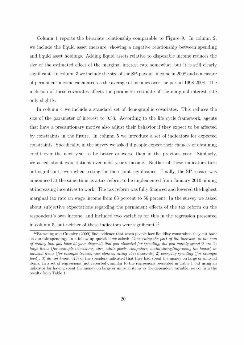
Column 1 reports the bivariate relationship comparable to Figure 9. In column 2,

we include the liquid asset measure, showing a negative relationship between spending

and liquid asset holdings. Adding liquid assets relative to disposable income reduces the

size of the estimated effect of the marginal interest rate somewhat, but it is still clearly

significant. In column 3 we include the size of the SP-payout, income in 2008 and a measure

of permanent income calculated as the average of incomes over the period 1998-2008. The

inclusion of these covariates affects the parameter estimate of the marginal interest rate

only slightly.

In column 4 we include a standard set of demographic covariates. This reduces the

size of the parameter of interest to 0.33. According to the life cycle framework, agents

that have a precautionary motive also adjust their behavior if they expect to be affected

by constraints in the future. In column 5 we introduce a set of indicators for expected

constraints. Specifically, in the survey we asked if people expect their chances of obtaining

credit over the next year to be better or worse than in the previous year. Similarly,

we asked about expectations over next year’s income. Neither of these indicators turn

out significant, even when testing for their joint significance. Finally, the SP-release was

announced at the same time as a tax reform to be implemented from January 2010 aiming

at increasing incentives to work. The tax reform was fully financed and lowered the highest

marginal tax rate on wage income from 63 percent to 56 percent. In the survey we asked

about subjective expectations regarding the permanent effects of the tax reform on the

respondent’s own income, and included two variables for this in the regression presented

in column 5, but neither of these indicators were significant.12

12Browning and Crossley (2009) find evidence that when people face liquidity constraints they cut backon durable spending. In a follow-up question we asked: Concerning the part of the increase [in the sumof money that you have at your disposal ] that you allocated for spending, did you mainly spend it on: 1)large items (for example televisions, cars, white goods, computers, maintaining/improving the house) orunusual items (for example travels, nice clothes, eating at restaurants) 2) everyday spending (for examplefood). 3) do not know. 67% of the spenders indicated that they had spent the money on large or unusualitems. In a set of regressions (not reported), similar to the regressions presented in Table 1 but using anindicator for having spent the money on large or unusual items as the dependent variable, we confirm theresults from Table 1.

20

Across the regressions in Table 1, we find that the marginal interest rate calculated from

pre-reform information is significant, both statistically and economically, in explaining the

propensity to spend the stimulus.

According to the theory the marginal interest rate should be better at predicting the

stimulus response than the average interest rate. In Table 2 we therefore compare the

ability of the average and the marginal interest rate to predict the spending response.13

Column 1 reproduces column 1 of Table 1, and column 2 shows results for the average

interest rate instead. The calculated average and marginal interest rates are, of course,

correlated and the average interest rate is therefore able to pick up the effect from column

1. In column 3 both measures are included; here, the marginal interest rate is significant,

while the average interest rate is insignificant. In columns 4-6 we repeat the estimations

including the full set of covariates from column 5 of Table 1 and confirm these results.

< Table 2 >

Estimations are based on OLS, and this can potentially lead to biased estimates as

most responses are either 0 or 1. To make sure that potential misspecification is not

driving the results, we have also reproduced the results using probit and tobit estimators,

which did not affect results (see Table A2 in the appendix). Furthermore, the specification

presented in Table 1 includes linear terms only. Figure 4 suggested that the propensity to

spend could be nonlinearly related to the size of the SP-payout. Another concern might

be that the realized marginal interest rate is in fact just picking up variations in income

across the persons/households in our sample. To address these concerns we repeated the

estimations including up to 4th order polynomials in the size of the SP-payout, in all

the income variables, and age. The inclusion of the polynomials affected the results only

marginally. Results are reported in Table A3 in the appendix. We also did an analysis

where the sample was split into four groups according to the income quartiles in 2008

13We have calculated the average interest rate by pooling across all deposit and loan accounts, respec-tively, and then picking the interest rate calculated from loan accounts, if the household has at leastone loan account, or the interest rate calculated from deposit accounts if the household has only depositaccounts.

21

and carried out regressions corresponding to column 5 in Table 1 separately for each of

these four sub-groups. The estimated effect of the interest gradient was almost identical

across the four subsamples confirming the observation that income is not a strong proxy

for liquidity constraints; these results are not reported but available upon request. As

an additional robustness check we also included respondents who did not take out the

SP-funds as non-spenders, but this did not affect results either; this is reported in Table

A4 in the appendix.

The average propensity to spend out of the stimulus was 65 percent according to our

survey, consistent with recent stimulus studies by Parker et al. (2013), Broda and Parker

(2014), and Agarwal and Qian (2014). Figure 9 suggests that the propensity to spend is

relatively high among individuals observed to have a low realized marginal interest rate in

2008, even though the theory predicts low responses in this case.14 This suggests that while

liquidity constraints may be important in explaining the response, there are arguably other

factors that are also important for explaining the response. One potential explanation for

this pattern is related to the size of the SP-payout. Previous studies have found that the

propensity to spend is high for small payout amounts but considerably smaller for large

payout amounts.15 The results reported in Table 1 suggest that size is important.

To get further insight into the importance of a size effect, we repeated the survey in

January 2012 and asked hypothetical questions about what the spending response would

have been had the SP-payout been 1,000 DKK, 10,000 DKK or 100,000 DKK (in random

order). The follow-up survey includes 3,135 persons from the original survey and was sup-

plemented with randomly selected new respondents to reach a total of 5,920 respondents.

We then matched these responses with the marginal interest rates from 2008 that we used

in Figure 9. The results are presented in Figure 10 and they show that the intercept,

i.e. the spending response at a zero interest rate, varies considerably with the size of the

14As noted earlier, 67% of the spenders indicated that their spending was mainly on large or unusualitems. To the extent that such items are durable goods, actual consumption in 2009 will be lower.

15For example, Hsieh (2003) finds that the propensity to consume out of (large and anticipated) pay-ments from Alaska’s Permanent Fund is smaller than the same individuals’ propensity to consumer outof (small and irregular) income tax refunds.

22

hypothetical pay-out. Changing the size of the hypothetical pay-out from 1,000 to 10,000

to 100,000 changes the intercept from 60% to 40% to 25%. While we do not claim that

this exhausts the list of explanations, these findings suggest that the level of the response

is clearly affected by the size of the pay-out. Interestingly, the 2008 marginal interest

rate gradient that we observed for the actual outcome in Figure 9 appears in all panels

in Figure 10 as well.16 It is also interesting to note, that the rate of extreme responses

(i.e. a spending share equal to either 0 or 1) decline with the size of the amount: the

fraction of extreme responses is 0.95, 0.83 and 0.49 for the 1.000, 10.000, and 100.000

hypothetical pay-out questions. This suggest that at least part of the reason for the high

rate of extreme responses in the survey, cf. figure 4, is related to the size of the pay-out.

< Figure 10 >

5.3 Why does liquidity constraint tightness vary across con-sumers?

The simple theory presented above suggests that preference heterogeneity or other person

fixed factors potentially play an important role in explaining the heterogeneity in the size

of the realized marginal interest rate across consumers. One advantage of the Danish

administrative register data is that it is possible to track people’s financial asset holdings

back to 1998. This enables us to check if the interest rate that we observe in 2008 is

correlated with the amount of liquid assets held by the same people in 1998. The idea that

we pursue in this section is that if the marginal interest rate observed in 2008 is correlated

with financial information recorded in 1998 then that suggests that the marginal interest

rate observed in 2008 is the result of factors that are fixed or at least persistent to a degree

that cannot be explained by what is usually thought of as transitory shocks.

Figure 11 depicts the bivariate relationship between the size of the marginal interest

rate in 2008 and the level of liquid assets in 1998. It shows a clear and significant negative

correlation between the marginal interest rate and the level of liquid assets to disposable

16We also performed the exercise for the subsample of 3,135 persons who participated in the originalsurvey and the results were unchanged.

23

income in 1998. To make sure that this relationship is not the result of events that are

particular to 1998 we also tried to correlate the marginal interest rate in 2008 with the

median of liquid assets to disposable income over the period 1998-2008 and we found that

the graph looked similar (not reported).

< Figure 11 >

The bivariate relationship is, of course, potentially misleading because the 1998 level

of assets may proxy for other variables measured in 2008. For example, Figure 7 showed

an equally strong relationship between the marginal interest rate in 2008 and the level of

liquid assets in 2008. Table 3 presents the results from a multivariate analysis of the ability

of historical asset levels to predict the current marginal interest rate. The first column in

Table 3 repeats the estimation from column 5, Table 1. In column 2 the interest rate is

regressed on all the covariates used in column 1 and on the level of liquid assets in 1998

and the interaction between the level of liquid assets in 1998 and the level of liquid assets

in 2008. The level of liquid assets in 1998 significantly predicts the marginal interest rate

in 2008 given the other covariates. In the next step we predict the marginal interest rate

using the estimates in column 2 and use the predicted marginal interest rate as a regressor

in the spending regression presented in column 3 where we also include as a separate

variable the residual variation in the interest rate. The marginal interest rate predicted

from the 1998 level of financial asset holdings is significant at the 1% level and much larger

in magnitude than in the basic estimation presented in column 1. These results suggest

that fixed or very persistent factors play an important role in predicting the marginal

interest rate and thereby the spending response to the stimulus policy.

< Table 3 >

One objection to this analysis could be that people observed with low levels of assets

in 1998 have been exposed to continuing bad luck in the labor market over the period.

In columns 4 and 5 we therefore repeat the exercise on a subsample of people that have

not been affected by unemployment at any point in the period 1998-2008. Results from

24

this subsample, consisting of more than half of the sample used in the other estimations,

confirm the previous findings. While these results do not rule out a role for historical

shocks so persistent that they impact behavior more than ten years after they appeared,

they suggest a role for heterogeneity that is persistent to a degree that cannot be accounted

for by shocks appearing within the typical duration of a business cycle.

We have also conducted other robustness checks of the results presented in table 3 (not

reported). In order to make sure that the results are not driven by just a single year with a

low level of liquid assets, we have tried to use the median of the entire time series of liquid

assets to disposable income over the period 1998-2008 in the prediction of the marginal

interest rate in the first stage regression. Results from this exercise were similar. In the

theory section, we noted that heterogeneity in marginal interest rates across consumers

could also be generated by differences in expected future income profiles. Therefore,

binding credit constraints could be a life cycle issue that is primarily relevant for the

young. However, when we narrow the sample to include only people who are 45 years or

older in 2008, we find that the results are almost unchanged.

6 Conclusion

Liquidity constraints have been the leading explanation for the observation of positive

spending responses in the literature studying effects of fiscal stimulus policies. This pa-

per has studied the effects of a Danish stimulus policy that transformed illiquid pension

wealth into liquid wealth, available for spending. The overall spending effect of this policy

of “giving people their own money” was significant. The survey responses indicate an

aggregate spending effect of about 1.8% of total private spending and 0.9% of GDP.

We examine the payout in the context of basic consumption theory extended with

heterogeneous interest rates. The theory predicts that the consumption response to a

stimulus is a function of the ex ante realized marginal interest rate. We test this proposi-

tion directly by merging, at the person level, survey responses with third-party reported

information from income-tax registers about all individual deposit and loan accounts held

25

by our survey respondents before the reform. Consistent with the theory we find that the

marginal interest rate is a robust predictor of the propensity to spend out of the stim-

ulus: a 1% point difference in the interest rate between consumers is associated with a

0.3-0.5% point difference in the propensity to spend. However, we also find large spending

responses for people who are unlikely to be affected by liquidity constraints which suggests

that other factors, including size effects, are arguably also important drivers of spending

responses.

Finally, we find that realized marginal interest rates in 2008 are strongly correlated

with consumers’ ratio of liquid assets to income more than a decade earlier. This suggests

that differences in the size of the realized marginal interest rate across people observed

in our data is the result of heterogeneity that is persistent to a degree that cannot be

explained by typical short lived shocks appearing within the duration of a typical business

cycle. This finding is consistent with a recent development of incorporating heterogeneity

into models of consumption behavior, for example as in Mankiw’s (2000) savers-spenders

model of fiscal policy and in the buffer-stock model of Carroll et al. (2013) introducing

heterogeneous time preference factors to explain responses to stimulus policies.

References

[1] Agarwal, Sumit and Qian, Wenlan. 2014, “Consumption and Debt Response to

Unanticipated Income Shocks: Evidence from a Natural Experiment in Singa-

pore (July 4, 2014)”. Available at SSRN: http://ssrn.com/abstract=2245351 or

http://dx.doi.org/10.2139/ssrn.2245351 .

[2] Agarwal, Sumit, Chunlin Liu and Nicholas S. Souleles. 2007. “The Reaction of Con-

sumer Spending and Debt to Tax Rebates—Evidence from Consumer Credit Data.”

Journal of Political Economy, 115(6): 986–1019.

[3] Alan, Sule and Martin Browning. 2010. ”Estimating Intertemporal Allocation Param-

eters using Synthetic Residual Estimation”. Review of Economic Studies, 77: 1231-

26

1261.

[4] Broda, Christian and Jonathan Parker. 2014. “The Economic Stimulus Payments of

2008 and the Aggregate Demand for Consumption”. Manuscript, MIT.

[5] Browning, Martin and Thomas Crossley. 2009. ”Shocks, Stocks and Socks: Smoothing

Consumption over a Temporary Income Loss”. Journal of the European Economic

Association, 7(6):1169-1192.

[6] Browning, Martin and Søren Leth-Petersen. 2003. ”Imputing Consumption from in-

come and wealth information” Economic Journal. 113(488), F282-301.

[7] Browning, Martin and Anna-Maria Lusardi. 1996. “Household Saving: Micro Theories

and Micro Facts.” Journal of Economic Literature, 34(4):1797-1855.

[8] Carroll, Christopher D., Jiri Slacalek, Kiichi Tokuoka. 2013. The Distribution of

Wealth and the Marginal Propensity to Consume. Manuscript, Johns Hopkins Uni-

versity.

[9] Chetty, Raj, John N. Friedman, Søren Leth-Petersen, Torben Heien Nielsen and Tore

Olsen. 2014. “Active vs. Passive Decisions and Crowd-out in Retirement Savings:

Evidence from Denmark”. Quarterly Journal of Economics, 129(3).

[10] Chetty, Raj, John N. Friedman, Tore Olsen and Luigi Pistaferri. 2011. “Adjustment

Costs, Firm Responses, and Micro vs. Macro Labor Supply Elasticities: Evidence

from Danish Tax Records.” Quarterly Journal of Economics, 126(2), pp. 749-804.

[11] Deaton, Angus. 1999. “Saving and Growth.” In Klaus Schmidt-Hebbel and Luis Ser-

ven (eds.), The Economics of Saving and Growth: Theory, evidence and implications

for policy, pp. 33-70, Cambridge: Cambridge University Press.

[12] Gross, David B., and Nicholas S. Souleles. 2002. “Do Liquidity Constraints and In-

terest Rates Matter for Consumer Behavior? Evidence from Credit Card Data.”

Quarterly Journal of Economics, 117(1): 149–85.

27

[13] Hsieh, Chang-Tai. 2003. “Do Consumers React to Anticipated Income Changes? Evi-

dence from the Alaska Permanent Fund.” American Economic Review, 93(1):397-405.

[14] Hurst, Erik. 2006. “Grasshoppers, Ants and Pre-Retirement Wealth: A Test of Per-

manent Income Consumers.” Manuscript, University of Chicago.

[15] Johnson, David S., Jonathan A. Parker, and Nicholas S. Souleles. 2006. “Household

Expenditure and the Income Tax Rebates of 2001.” American Economic Review,

96(5): 1589–1610.

[16] Kaplan, Greg and Violante, Gianluca. 2013. “A Model of the Consumption Response

to Fiscal Stimulus Payments.” Manuscript, August.

[17] Kleven, Henrik Jacobsen, Martin Knudsen, Claus Thustrup Kreiner, Søren Pedersen,

Emmanuel Saez. 2011. “Unwilling or Unable to Cheat? Evidence from a Tax Audit

Experiment in Denmark.” Econometrica, 79, pp. 651–692

[18] Kreiner, Claus Thustrup, David Dreyer Lassen, Søren Leth-Petersen. 2014. “Measur-

ing the Accuracy of Survey Responses using Administrative Register Data: Evidence

from Denmark”. Forthcoming in Improving the Measurement of Household Consump-

tion Expenditures, eds. Christopher Carroll, Thomas Crossley, John Sabelhaus, NBER

Book Series, Studies in Income and Wealth.

[19] Leth-Petersen, Søren. 2010. “Intertemporal Consumption and Credit Constraints:

Does Consumption Respond to An Exogenous Shock to Credit?”. American Economic

Review, 100(3), pp. 1080-1103.

[20] Mankiw, N. Gregory. 2000. “The Savers-Spenders Theory of Fiscal Policy.” American

Economic Review, 90(2), pp. 120–25.

[21] Parker, Jonathan A., Nicholas S. Souleles, David S. Johnson and Robert McClelland.

2013. “Consumer Spending and the Economic Stimulus Payments of 2008”. American

Economic Review, 103(6), pp. 2530–2553.

28

[22] Sahm, Claudia, Matthew Shapiro, Joel Slemrod. 2010. ”Household Response to the

2008 Tax Rebates: Survey Evidence and Aggregate Implications” Tax Policy and the

Economy, 24, pp. 69-110.

[23] Shapiro, Matthew D., and Joel Slemrod. 2009. “Did the 2008 Tax Rebates Stimulate

Spending?” American Economic Review, 99(2): 374–379.

[24] Shapiro, Matthew D., and Joel Slemrod. 2003. “Consumer Response to Tax Rebates.”

American Economic Review, 93(1): 381–96.

[25] Shapiro, Matthew D., and Joel Slemrod. 1995. “Consumer Response to the Timing of

Income: Evidence from a Change in Tax Withholding.” American Economic Review,

85(1): 274–83.

[26] Souleles, Nicholas S. 1999. “The Response of Household Consumption to Income Tax

Refunds.” American Economic Review, 89(4), pp. 947–58.

[27] Zeldes, Stephen P. 1989. “Consumption and Liquidity Constraints: An Empirical

Investigation.” Journal of Political Economy, 97(2), pp. 305–46.

29

 Figure  1:  Newspaper  coverage  of  SP  scheme

NOTE:  Number  of  articles  about  SP-­‐savings  scheme  in  national  newspapers.

SOURCE:  Infomedia.

Panel  A Panel  B

Figure  2:  Stimulus  policy  and  preference  heterogeneity

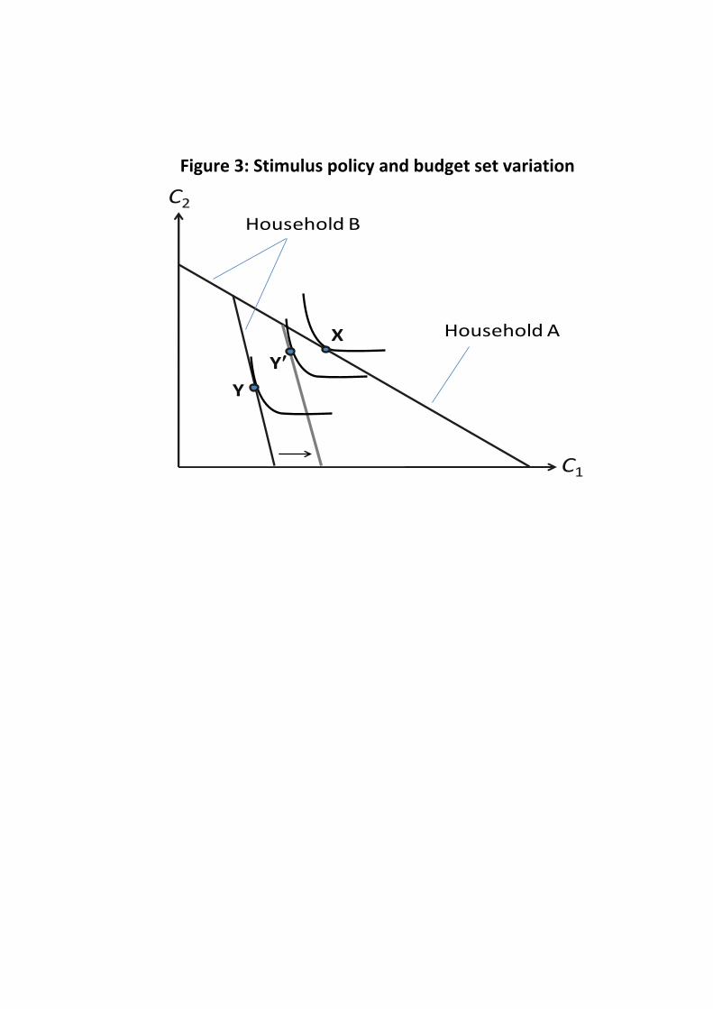
Figure  3:  Stimulus  policy  and  budget  set  variation

C2

C1

X

YYʹ′

Household  A

Household  B

Figure  4:  Spending  responses  and  the  size  of  the  SP  payout

Figure  5:  Distribution  of  marginal  interest  rates  across  households

Figure  6:  Calculated  interest  rate  and  the  corresponding  reported  interest  rate

Figure  7:  Marginal  interest  rate  and  ln(income)  (A)  and  liquid  assets  (B)

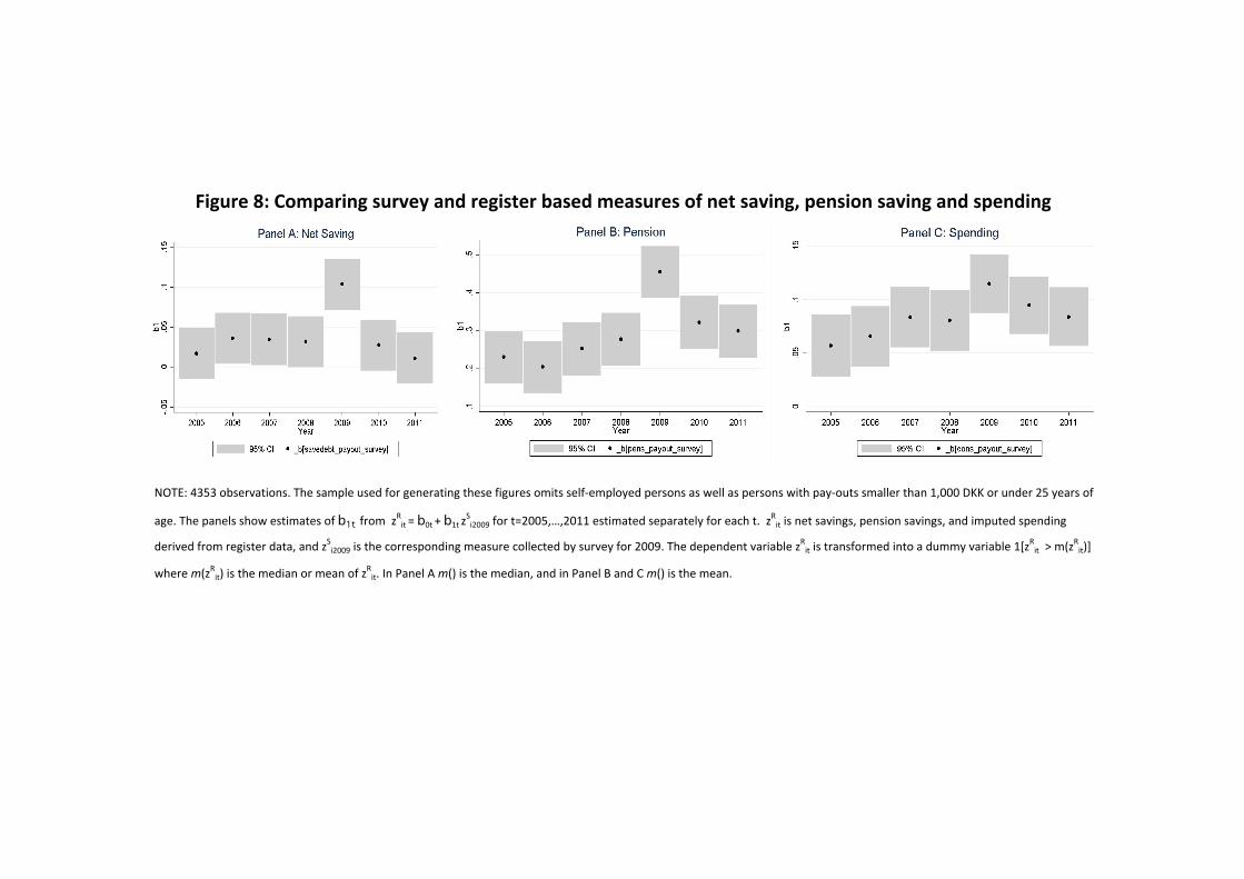
 Figure  8:  Comparing  survey  and  register  based  measures  of  net  saving,  pension  saving  and  spending

     NOTE:  4353  observations.  The  sample  used  for  generating  these  figures  omits  self-­‐employed  persons  as  well  as  persons  with  pay-­‐outs  smaller  than  1,000  DKK  or  under  25  years  of

     age.  The  panels  show  estimates  of  b1t from    zRit  =  b0t  +  b1t  zSi2009  for  t=2005,…,2011  estimated  separately  for  each  t.    zRit  is  net  savings,  pension  savings,  and  imputed  spending  

     derived  from  register  data,  and  zSi2009  is  the  corresponding  measure  collected  by  survey  for  2009.  The  dependent  variable  zRit  is  transformed  into  a  dummy  variable  1[zRit    >  m(zRit)]  

     where  m(zRit)  is  the  median  or  mean  of  zRit.  In  Panel  A  m()  is  the  median,  and  in  Panel  B  and  C  m()  is  the  mean.

Figure  9:  Household  propensity  to  spend  and  marginal  interest  rate

Figure  10:  Household  propensity  to  spend  and  marginal  interest  rate  for  hypothetical  SP  payouts  equal  to  1,000  DKK  (A),  10,000  DKK  (B),  and  100,000  DKK  (C)

Figure  11:  Marginal  interest  rate  2008  and  liquid  assets  in  1998

Figure  A1:  The  SP-­‐letter

Table  1.  Spending  share  regressed  on  covariates  (OLS)(1) (2) (3) (4) (5)

LiquidityMarginal  interest  rate,  2008 0.518 *** 0.368 *** 0.361 *** 0.332 *** 0.332 ***Liquid  assets  /  disp  income,  2008 -­‐0.064 *** -­‐0.054 *** -­‐0.039 ** -­‐0.039 **Size  EffectLn(net  SP) -­‐0.075 *** -­‐0.074 *** -­‐0.074 ***Income  controlsLn(income),  register -­‐0.009 -­‐0.021 -­‐0.020Ln(permanent  income) -­‐0.042 -­‐0.018 -­‐0.019sd[ln(income)] -­‐0.017 -­‐0.023 -­‐0.023Income  developed  better,  2009  (d) 0.025 0.017 0.024Income  developed  worse,  2009  (d) -­‐0.005 -­‐0.008 -­‐0.007Demographic  controlsAge -­‐0.002 ** -­‐0.002 **Woman    (d) 0.026 0.026Single  (d) 0.007 0.007Number  of  children 0.022 ** 0.021 **Education,  short  (d) -­‐0.006 -­‐0.006Education,  medium  (d) -­‐0.020 -­‐0.020Education,  long  (d) -­‐0.046 -­‐0.046Owner  (d) 0.023 0.022Expected  ConstraintsChange  E[credit  possibility  2010]<0,  2009  (d) 0.013Change  E[credit  possibility  2010]>0,  2009  (d) -­‐0.004Change  E[income  2010]>0,  2009  (d) -­‐0.020Change  E[income  2010]<0,  2009  (d) -­‐0.001Taxreform  =>  permanent  income  increase  (d) -­‐0.011Taxreform  =>  permanent  income  decrease  (d) -­‐0.037

N 5055 5055 5055 5055 5055(d)  for  discrete  change  of  dummy  variable  from  0  to  1.    *  p<0.05,  **  p<0.01,  ***  p<0.001

Table  2.  Spending  share  regressed  on  covariates  (OLS)  (1) (2) (3) (4) (5) (6)

LiquidityMarginal  interest  rate,  2008 0.518 *** 0.544 *** 0.332 *** 0.371 ***Average  interest  rate,  2008 0.584 ** -­‐0.115 0.264 -­‐0.178Liquid  assets  /  disp  income,  2008   -­‐0.039 ** -­‐0.050 *** -­‐0.040 **Size  EffectLn(net  SP) -­‐0.074 *** -­‐0.073 *** -­‐0.074 ***Income  controlsLn(income),  register       -­‐0.020   -­‐0.023   -­‐0.021  Ln(permanent  income)     -­‐0.019   -­‐0.017 -­‐0.018  sd[ln(income)]     -­‐0.023   -­‐0.022   -­‐0.023  Income  developed  better,  2009  (d)       0.024   0.025   0.024  Income  developed  worse,  2009  (d)       -­‐0.007   -­‐0.005   -­‐0.007  Demographic  controlsAge     -­‐0.002 ** -­‐0.002 ** -­‐0.002 *Woman    (d)       0.026   0.026   0.026  Single  (d)       0.007   0.004   0.007  Number  of  children       0.021 ** 0.022 *** 0.021 **Education,  short  (d)       -­‐0.006   -­‐0.008   -­‐0.006  Education,  medium  (d)       -­‐0.020   -­‐0.023   -­‐0.020  Education,  long  (d)       -­‐0.046   -­‐0.051 * -­‐0.046  Owner  (d)       0.022   0.023   0.020  Expected  ConstraintsChange  E[credit  possibility  2010]<0,  2009  (d)       0.013   0.017   0.013  Change  E[credit  possibility  2010]>0,  2009  (d)       -­‐0.004   -­‐0.002   -­‐0.005  Change  E[income  2010]>0,  2009  (d)       -­‐0.020   -­‐0.018   -­‐0.019  Change  E[income  2010]<0,  2009  (d)       -­‐0.001   0.001   -­‐0.001  Taxreform  =>  permanent  income  increase  (d)       -­‐0.011   -­‐0.012   -­‐0.011  Taxreform  =>  permanent  income  decrease  (d)       -­‐0.037   -­‐0.039   -­‐0.037  

N 5055   5055   5055   5055   5055   5055  (d)  for  discrete  change  of  dummy  variable  from  0  to  1.    *  p<0.05,  **  p<0.01,  ***  p<0.001

Table  3.  Spending,  the  interest  rate  and  historical  asset  levels

(1) (2) (3) (4) (5)LiquidityMarginal  interest  rate,  2008 0.332 ***Marginal  interest  rate,  2008,  predicted 2.048 ** 3.162 **Marginal  interest  rate,  2008,  residual 0.311 *** 0.262 *Liquid  assets  /  disp  income,  2008 -­‐0.039 ** -­‐0.046 *** 0.035 -­‐0.044 *** 0.080Liquid  assets  1998Liquid  assets  /  disp  income,  1998 -­‐0.024 *** -­‐0.020 ***(LiqAss/disp,1998)*(LiqAss/disp,2008) 0.014 *** 0.012 ***Size  effect Yes Yes Yes Yes YesExpected  constraints Yes Yes Yes Yes YesIncome  controls Yes Yes Yes Yes YesDemographic  controls Yes Yes Yes Yes Yes

N 5055 5055 5055 2698 2698*  p<0.05,  **  p<0.01,  ***  p<0.001

Share Interest  Rate Share Interest  Rate Share

All  individuals Never  unemployedSpending Spending Spending

Table  A1.    Means  of  characteristics(1) (2) (3) (4) (5)

RespondentsRespondents,  

no  pay-­‐outt-­‐value,                (1)-­‐(2)

Non-­‐respondents

t-­‐value,      (1)-­‐(4)

LiquidityMarginal  interest  rate,  2008 0.100 0.103 -­‐0.50 0.103 -­‐1.90Liquid  assets  /  disp  income,  2008 0.420 0.409 0.25 0.421 -­‐0.01Size  EffectNet  Payout 9967.000 8625.700 3.37 8633.200 12.38Gross  Payout 16236.000 13968.000 3.22 13988.000 11.85Income  controlsLn(income),  register 12.712 12.618 1.87 12.554 11.26Ln(permanent  income) 12.583 12.478 2.54 12.442 12.38sd[ln(income)] 0.249 0.4263 -­‐2.26 0.423 -­‐7.48Demographic  controlsAge 45.070 45.699 -­‐0.72 44.655 1.80Woman    (d) 0.518 0.503 0.39 0.479 3.94Single  (d) 0.219 0.277 -­‐1.81 0.318 -­‐11.26Number  of  children 0.899 0.636 3.16 0.731 7.98Education,  short  (d) 0.447 0.422 0.65 0.449 -­‐0.26Education,  medium  (d) 0.219 0.156 1.96 0.151 8.87Education,  long  (d) 0.100 0.116 -­‐0.68 0.066 6.13Owner  (d) 0.751 0.694 1.72 0.545 22.34

N 5055 173 5171(d)  for  discrete  change  of  dummy  variable  from  0  to  1.    *  p<0.05,  **  p<0.01,  ***  p<0.001

Table  A2.  Spending  share  regressed  on  covariatesOLS Tobit Probit OLS Tobit Probit

LiquidityMarginal  interest  rate,  2008 0.518 *** 0.519 *** 0.573 *** 0.332 *** 0.342 *** 0.395 ***Liquid  assets  /  disp  income,  2008 -­‐0.039 ** -­‐0.038 ** -­‐0.039 **Size  EffectLn(net  SP) -­‐0.074 *** -­‐0.095 *** -­‐0.081 ***Income  controlsLn(income),  register -­‐0.020 -­‐0.019 -­‐0.026Ln(permanent  income) -­‐0.019 -­‐0.017 -­‐0.012sd[ln(income)] -­‐0.023 -­‐0.017 -­‐0.028Income  developed  better,  2009  (d) 0.024 0.026 0.027Income  developed  worse,  2009  (d) -­‐0.007 -­‐0.008 -­‐0.010Demographic  controlsAge -­‐0.002 ** -­‐0.002 * -­‐0.002 *Woman    (d) 0.026 0.023 0.026Single  (d) 0.007 0.007 0.015Number  of  children 0.021 ** 0.023 ** 0.020 **Education,  short  (d) -­‐0.006 -­‐0.005 -­‐0.003Education,  medium  (d) -­‐0.020 -­‐0.021 -­‐0.020Education,  long  (d) -­‐0.046 -­‐0.051 -­‐0.049Owner  (d) 0.022 0.025 0.018Expected  ConstraintsChange  E[credit  possibility  2010]<0,  2009  (d) 0.013 0.015 0.012Change  E[credit  possibility  2010]>0,  2009  (d) -­‐0.004 -­‐0.008 0.002Change  E[income  2010]>0,  2009  (d) -­‐0.020 -­‐0.021 -­‐0.024Change  E[income  2010]<0,  2009  (d) -­‐0.001 -­‐0.001 -­‐0.001Taxreform  =>  permanent  income  increase  (d) -­‐0.011 -­‐0.011 -­‐0.006Taxreform  =>  permanent  income  decrease  (d) -­‐0.037 -­‐0.037 -­‐0.035

N 5055 5055 5055 5055 5055 5055(d)  for  discrete  change  of  dummy  variable  from  0  to  1.    *  p<0.05,  **  p<0.01,  ***  p<0.001

Table  A3.  Spending  share  regressed  on  covariates  (OLS)(1) (2)

LiquidityMarginal  interest  rate,  2008 0.332 *** 0.336 ***Liquid  assets  /  disp  income,  2008 -­‐0.039 ** -­‐0.043 **Size  effectLn(net  SP) -­‐0.074 *** -­‐0.021[Ln(net  SP)]^2 -­‐0.003[Ln(net  SP)]^3 0.000[Ln(net  SP)]^4 -­‐0.000Income  controlsLn(income),  register -­‐0.020 -­‐0.037Ln(income)^2,  register 0.053Ln(income)^3,  register -­‐0.008Ln(income)^4,  register 0.000Ln(permanent  income) -­‐0.019 33.867Ln(permanent  income)^2 -­‐4.171Ln(permanent  income)^3 0.228Ln(permanent  income)^4 -­‐0.005Other  income  controls Yes YesDemographic  controlsAge -­‐0.002 ** -­‐0.078Age^2 0.003Age^3 -­‐0.000Age^4 0.000Other  demographic  controls Yes YesExpected  constraints Yes Yes

N 5055 5055  *  p<0.05,  **  p<0.01,  ***  p<0.001

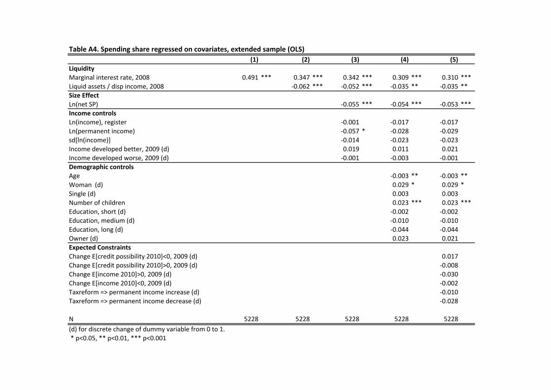
Table  A4.  Spending  share  regressed  on  covariates,  extended  sample  (OLS)(1) (2) (3) (4) (5)

LiquidityMarginal  interest  rate,  2008 0.491 *** 0.347 *** 0.342 *** 0.309 *** 0.310 ***Liquid  assets  /  disp  income,  2008 -­‐0.062 *** -­‐0.052 *** -­‐0.035 ** -­‐0.035 **Size  EffectLn(net  SP) -­‐0.055 *** -­‐0.054 *** -­‐0.053 ***Income  controlsLn(income),  register -­‐0.001 -­‐0.017 -­‐0.017Ln(permanent  income) -­‐0.057 * -­‐0.028 -­‐0.029sd[ln(income)] -­‐0.014 -­‐0.023 -­‐0.023Income  developed  better,  2009  (d) 0.019 0.011 0.021Income  developed  worse,  2009  (d) -­‐0.001 -­‐0.003 -­‐0.001Demographic  controlsAge -­‐0.003 ** -­‐0.003 **Woman    (d) 0.029 * 0.029 *Single  (d) 0.003 0.003Number  of  children 0.023 *** 0.023 ***Education,  short  (d) -­‐0.002 -­‐0.002Education,  medium  (d) -­‐0.010 -­‐0.010Education,  long  (d) -­‐0.044 -­‐0.044Owner  (d) 0.023 0.021Expected  ConstraintsChange  E[credit  possibility  2010]<0,  2009  (d) 0.017Change  E[credit  possibility  2010]>0,  2009  (d) -­‐0.008Change  E[income  2010]>0,  2009  (d) -­‐0.030Change  E[income  2010]<0,  2009  (d) -­‐0.002Taxreform  =>  permanent  income  increase  (d) -­‐0.010Taxreform  =>  permanent  income  decrease  (d) -­‐0.028

N 5228 5228 5228 5228 5228(d)  for  discrete  change  of  dummy  variable  from  0  to  1.    *  p<0.05,  **  p<0.01,  ***  p<0.001