literature review, database and...
TRANSCRIPT
LITERATURE REVIEW,DATABASE AND METHODOLOGY
C. N. Krishnankutty “Demand, supply and price of teakwood in Kerala” Thesis. Department of Economics, Dr. John Matthai Centre, University of Calicut, 1997
CHAPTER 2
LITERATURE REVIEW,
DATABASE AND METHODOLOGY
A review on the related studies on demand, supply and price of
timber is done in this chapter. The methodology adopted in the
present study and the sources of data are also described here.
2.1 Review of Literature
This section consists of a review on the studies in India and
other countries.
2.1.1 Studies in India
Studies on demand, supply and price aspects of timber are very
few in India. An assessment of the growing stock of wood in the
forests of Kerala and annual availability was made for the year 1970 by
chandrasekharanl. A rough estimate of the demand for pulpwood in
Kerala and supply from forests for the year 1982 was made by
~ a r u n a k a r a n ~ . The pioneering work on the wood economy of Kerala
covering sector-wise demand for timber and fuelwood and supply
from forests as well as non-forest sources has been carried out for the
reference year 1987-88 by the author3 and published as 'demand
and supply of wood in Kerala and their future trends'. In the above
l Chandrasekharan, C. (1973). op.cit.
Karunakaran, C. K. (1982). Demand versus supply of important raw
materials from forests in Kerala State (Draft). Kerala Forest Department, Thiruvananthapuram.
Krishnankutty, C. N. (1990). Demand and supply of wood in Kerala and their future trends. KFRI Research Report 67, Kerala Forest Research
Instutute, Peechi.
study, the demand for construction timber, industrial wood and
fuel by different sectors in Kerala was estimated and the various
sources of supply were identified. There are also some studies which
had been done during the last few years in Kerala. Examples are,
availability of plywood logs from forests4, household fuelwood
consumption and its variation among villages located in different
geographical regions5, rural energy and use-pattern in Southern
~ e r a l a ~ and demand and supply of rubberwood in 1ndia7. Studies on
demand and supply of wood in other states in India reported in the
literature are very few. The wood-balance study conducted by the
conducted by the West Bengal Forest ~ e ~ a r t m e n t ~ is one among
them. Most of these studies dealt with demand and supply of wood,
which include industrial wood and fuel, in a particular year.
i) Kerala Forest Research Institute (1977). Availability of wood raw material for plywood industry (Kerala - Karnataka Region). KFRI Research Report
2(1), Peechi.
ii) Kerala Forest Research Institute (1978). Availability of wood raw mate- rial for plywood industry (North-Eastern Region). KFRI Research Report 2(2), Peechi.
Thampi, K. B. (1983). Pattern of domestic energy consumption in rural
Kerala : A study of selected villages. M.Phi1. Dissertation. Centre for
Development Studies, Thiruvananthapuram.
State Planning Board (1986). Rural energy generation and use-pattern:
Southern Kerala. Government of Kerala, Thiruvananthapuram.
Haridasan, V. and Sreenivasan, K. G. (1985). Rubberwood: A study of supply and demand in India. Rubber Board Bulletin, 20(4), 19-21.
West Bengal Forest Department (1987). Wood balance study : West Bengal.
Office of the Chief Conservator of Forests, Calcutta.
There are some studies on timber prices. In a study by
ICrishnankuttyg et al., timber prices up to the year 1981-82 were
analysed for certain timbers in Kerala. Timber price movements
in different periods in Kerala were examined in another study by
~ r i s h n a n k u t t ~ l ~ after updating the data till 1984-85. There are
some studies on timber prices in other states in India. They prima-
rily dealt with price variation between different size classesll or
short-term fluctuation of firewood prices12. Another study by
Sagar and ~ a h e n d r a ' ~ examined the inter-market price variation of
sal timber in Orissa and projected the prices using regression
model based on 10 years annual data.
2.1.2 Studies in other countries
Most of the studies in this area have been done abroad. The
relevant studies are grouped into studies on (i) timber demand,
supply and market and (ii) timber price and forecasting, and
reviewed in the following two sub-sections.
Krishnankutty, C. N., Rugmini, P. and Rajan, A. R. (1985). Analysis of factors
influencing timber prices in Kerala. KFRI Research Report No. 34. Kerala Forest Research Institute, Peechi.
I0 Krishnankutty, C. N. (1989). Long-term price trends of timber in Kerala.
Indian J. of For., 12(1), 7-12.
l 1 i) Suri, S. K. (1973). Comprehensive price trend studies of five commercially
important timber species logs - Narainpur Depot (Madhya Predesh) Indian
For., 99(8) : 510-515.
ii) Suri, S. K. (1974). Price trend studies on teak logs - Taku Depot (Madhya
Predesh). Indian For., 100(4) : 235-245.
l 2 Mathur, R. S., Sagar, S. R. and Mahendra, A. K. (1984). Price trends of firewood in Haryana. Indian For., 1 lO(10) : 973-981.
l 3 Sagar, S. R. and Mahendra, A. K. (1986). Price trends of sal timber in
Orissa. Indian For., 112(12), 1080-1087.
Studies on timber demand, supply and market
A large number of studies have been done abroad on this topic.
McKillop et aZ.,l4 estimated demand function for plywood, taking
quantity of plywood demanded as regressand and number of housing
started, industrial production index, hourly wage rate of carpenters,
plywood and building board prices lagged by one year as regressors
in United States. In an econometric study for US hardwood timber,
Luppoldls estimated the model taking the quantity demanded as a
function of the lagged rates of interest, a time trend, lagged prices
of hardwood timber, wooden furniture and hardboard and lagged wage
rates in the furniture industry, using data for the period from 1960
to 1979. Adams and lack well'^ estimated US timber and plywood
demand taking the quantity demanded in construction as a function
of total US housing started and the ratio of past plywood prices to
past timber prices, using data for the period from 1949 to 1969.
A long-term domestic demand function for Bangladesh was
estimated by McKillop and sarkar17 with quantity of timber
demanded as a function of real price of timber, population and a
time trend, using annual data from 1960 to 1982 and predicted the
demand for timber to the year 2025.
l4 Mckillop, W. L. M., Stuart, T. W. and Geissles, P. J. (1980). Competition
between wood products and substitute structural products: An econometric analysis. For. Sci., 26(1): 134-148.
lS Luppold, W. (1984). An econometric study of the U.S. hardwood timber market. For. Sci., 30(4): 1027-1038.
l 6 Adams, F. G. and Blackwell, J. (1973). An econometric model of the US forest products industry. For. Sci., 19(1): 82-96.
l7 McKillop, W. and Sarkar, A. (1992). Normative supply modelling and forest policy analysis in a developing economy. J. of world forest resource
management, 6(1): 85-98.
In a global study, Buongiorno et al.,lg estimated income and
price elasticities of demand for sawnwood and wood-based panels,
using data from 1963 to 1973 from 43 countries in a combined cross-
sectionltime series analysis. ~ c ~ i l l o ~ l ~ estimated Japanese demand
for US and Canadian timber using quarterly data for the period from
1950 to 1970.
~ r e b e r ~ O estimated an econometric model to analyse timber
supply in Virginia using inventory data from the U.S. Forest
Service. The long-term supply response of the regulated forest
developed by Clawson was applied by ~ ~ d e ~ ' to the Pacific North-
West region of the United States. Hyde estimated long-run
supply curves based upon the selection of a management regime
that maximised the present net worth of stumpage returns. Greber
and developed a timber market model. They estimated
product demand functions for pulpwood, hardwood saw - logs and
softwood saw - logs, using market data for the period from 1960
l8 Buongiomo, J., Chou, J. H, and Stone, R. S. (1979). A monthly model of the United States demand for softwood timber imports. Fox Sci., 25(4): 641-655.
l9 McKillop, W. (1973). Structural analysis of Japanese-North American trade in forest products. For. Sci., 19(1): 63-74.
Greber, B. J. (1983). Development of a joint product timber supply model.
Ph.D. Thesis, Va Polytech Inst. and State Univ., Blacksburg.
21 Hyde, W. F. (1980). Timber supply, land allocation a n d economic
eficiency. John Hopkins Univ. Press, Baltimore.
22 Greber, B. J and Wisdom, H. W. (1985). A timber market model for analysing
roundwood product interdependencies. FOE Sci., 3 l(1): 164-1 79.
to 1979. Hultkrantz and ~ r o n s s o n ~ ~ made an econometric study on
the supply of roundwood from private forest lands in Sweden, using
data from 1961 to 1984.
~ 0 1 - i ~ ~ investigated the supply and demand relationship, using
time series data relating to the Japanese timber market for the
period from 1960 to 1979. Chou and ~ u o n g i o r n o ~ ~ estimated own-
price and cross-price elasticities of US demand for imported
plywood, using monthly imports for the period from 1974 to
1979. ~ r a n n l u n d ~ ~ et d. presented an econometric analysis of the
sawn timber and pulpwood market in Sweden based on time-series
data, covering the period from 1953 to 198 1.
~ o b i n s o n ~ ~ estimated an econometric model for stumpage
market, using data for the period from 1947 to 1967. The demand
was expressed as a function of the real price of timber, freight
rates, the real value of residential construction per dwelling unit
and the number of dwelling units. In Adams and Haynes' US
23 Hultkrantz, L. and Aronsson, T. (1989). Factors affecting the supply and
demand of timber from private non-industrial lands in Sweden: An econometric
study. For. Sci., 35(4): 946-961.
24 Mori, Y. (1981). An econometric model of the Japanese timber market. XVII IUFRO World Congress, Kyoto, Japan.
25 Chou, J. and Buongiorno, J. (1983). United States demand for hardwood plywood imports by country of origin. For. Sci., 29(2): 225-237.
26 Brannlund, R., Johnson, P. 0. and Lofgren, K. G. (1985). An econometric analysis of aggregate sawn timber and pulpwood supply in Sweden. For. Sci., 31(3): 595-606.
27 Robinson, V. L. (1974). An econometric model of softwood timber and
stumpage markets: 1946-1967. Fox Sci., 20(1): 171-179.
timber assessment market model2*, the volume of available timber
was explicitly taken into account in the equations for regional
stumpage supply from private lands. This model was used to make
projections for the U.S. stumpage demand and supply.
Studies on timber price and forecasting
Huang and ~ u o n g i o r n o ~ ~ developed a model of market value
for tracts of timber sold at auction for a minimum appraised value
when a substantial number of the tracts offered did not receive a
bid. In a study by ~ r a z i e r ~ ~ for the Californian pine region, the bid
price was estimated as a function of the number of bidders
competing for each sale and the appraised price. Adams and
~ a ~ n e s ~ l presented an aggregate regional model of the national
forest timber supply in the determination of regional stumpage
price and harvest volume in the Western United States.
Components of the model described the distribution of volume sold
and bid price.
28 Adams, D. M. and Haynes, R. W. (1980). The 1980 softwood timber
assessment market model: Structure, projections and policy simulations. For. Sci. Monograph, 22:64p.
29 Huang, F. M. and Buongiorno, J. (1986). Market value of timber when some
offerings are not sold: Implications for appraisal and demand analysis. For.
Sci., 32(4):845-854.
30 Frazier, G. D. (1967). The relationship between Forest Service timber sales behavior and the structure of the Californian pine timber industry. Ph.D. Thesis, Yale Univ., New Haven, Conn.
31 Adams, D. M. and Haynes, R. W. (1989). A model of national forest timber supply and stumpage markets in the Western United States. For. Sci., 35(2):
40 1-424.
Studies in U S A ' ~ and ~ a ~ a n ' ' analysed the timber price
movement and their causative factors. Brazee and ~ e n d e l s o h n ~ ~
developed optimal reservation prices by age treating prices as
exogenous. In order to calculate the size of historic price
fluctuations, they used stumpage prices of douglas-fir for the
period from 1975 to 1984 and loblolly pine for the period from
1970 to 1979. These nominal prices were deflated using the GNP
deflator to 1986 constant dollars. In the model of Hardie et
prices were made as a function of calendar time and optimum
rotation lengths. ~ h a n ~ ~ ~ treated timber prices and production
costs as fixed parameters which did not vary with either harvest age
or calendar time. Clements et described a roundwood supply
and price assessment model for regional forest products markets.
~ o l l a n d ' ~ tried to show how timber price had risen while total
timber consumption expanded only moderately during the period
from 1920 to 1955. He further predicted the price index for
timber for the year 20 10.
32 Barnett, H. J. and Morse, C. (1963). op. cit.
33 Nomura, I. and Yikutake, K. (1981). op. cit.
34 Brazee, R. and Mendelsohn, R. (1988). Timber harvesting with fluctuating prices. For. Sci., 34(2): 359-372.
35 Hardie, L. W., Daberkow, J. N. and McConnell, K. E. (1984). A timber
harvesting model with variable rotation lengths. For. Sci., 30(2): 5 11-523.
36 Chang, S. J. (1981). Determination of the optimal growing stock and cutting
cycle for an uneven-aged stand. For. Sci., 27(4): 739-744.
37 Clements, S. E., Leuschner, W. A., Hoganson, H. and Wisdom, H. W. (1988). A local roundwood supply and price assessment model. Can.J.For.Res.,
18:1563-1569.
38 Holland, I. I. (1960). An explanation of changing timber consumption and
prices. For. Sci., 6(1): 171-192.
The Box-Jenkins time series approach3' has been used quite
extensively to predict the price in many other cases, but rarely in
timber price. Cheng and ~ e n ~ O tested the Box-Jenkins models to
predict timber prices of selected species of Taiwan. Oliveira et
al . ," invest igated the potentiality of the Box-Jenkins
autoregressive integrated moving average (ARIMA) model for
forecasting various timber prices (timber cash prices and their
basis series). The sample period for the weekly price series was
f rom January 1973 to December 1974, result ing in 103
observations. By using weekly observations, relatively accurate
forecasts could be obtained for timber prices with ARIMA models.
The results indicated that forecasting cash price had more merit
than forecasting the basis price.
The studies, which have been reviewed, focused on estimation
of demand or supply or market models. Some studies dealt with
prices alone. All these studies done abroad had access to time
series data. A few studies done in India have projected the demand
and supply of certain industrial wood using data for a single year and
based on certain assumptions. Hitherto, no comprehensive study on
demand, supply and price behaviour of timber has been done in India.
The present study on 'demand, supply and price of teakwood in Kerala'
is an attempt on a regional basis in this direction.
39 Box, G. E. P. and Jenkins, G. M. (1976). Time Series Analysis, Forecasting
and Control. (2nd ed.) San Francisco: Holden-Day.
40 Cheng, C. C. and Jen, J. A. (1980). Studies on the fluctuation and
prediction of timber prices in Taiwan. Taiwan Forestry Research Institute
Bulletin 338. Taipei, Taiwan.
41 Oliveira, R. A., Buongiorno, J. and Kmiotek, A. M. (1977). Time series forecasting models of timber cash, futures and basis prices. For. Sci., 23(2):
268-280.
2.2 Database
This study focuses on sector-wise demand for teakwood and
source-wise supply, prices of teakwood in the government timber
depots, regional variations in prices, long-term trends in prices and
forecasting. For estimating the share of teakwood in the total
timber supply, an assessment of the demand and supply of all
timbers in Kerala was necessary. For comparing the price trends of
teakwood with those of other timbers, it was necessary to consider
the prices of certain important timbers also.
The database of demand and supply of teakwood is the data
collected in an earlier study, by the author42, funded by the World
Bank aided Kerala Social Forestry Project. In the above study, both
timber and fuelwood were considered. But the emphasis in the
study was to obtain aggregate estimates for all timbers together and
fuelwood. The study did not aim at estimating the sector-wise
demand for teakwood or any other individual timber. The raw data
on teakwood collected in the course of the above study have been
used in the present study. The sector-wise demand and source-wise
supply of teakwood were estimated from these data. The concepts
and method of estimation of demand and supply in this study are
described in the next section.
The database of prices is mainly the monthly auction files and
registers maintained in the government timber depots. The Kerala
Government set up timber depots for sale of timber obtained from
42 Krishnankutty, C. N. (1990). op. c i f .
teak plantations and forests43. The depots are managed by the
Kerala Forest Department. Teakwood and other timbers obtained
from forests and plantations are transported to the timber depots.
At the depots, the logs are classified according to species, quality
and dimension". The classified logs are then grouped into lots
which are then put up for auction, usually every month. Auctions
are conducted for each lot and price is realised for each lot in the
monthly auction.
Price data available in the monthly auction files for the period
from 1975-76 to 1993-94 were collected from 23 depots out of 26
depots currently functioning45. Appendix 2 gives the list of the
government depots from which data were collected. Since the data
prior to 1975-76 were not available in most of the depots, the
average annual prices given in various Divisional Forest Working
were compiled for the period from 1956-57 to 1974-75.
Data on total quantity of teakwood sold through all the
government depots together and production from Kerala forests
during the period from 1956-57 to 1992-93 were compiled from
the Administration Reports of various years of the Kerala Forest
43 There are different sources of timber supply in Kerala. However, an organised market exists only for timber supplied from government forests.
Therefore, the study on prices has been confined to the timber supplied from Kerala forests.
44 For criteria for classification of logs, see Appendix 1.
45 Clearfelling was discontinued in Kerala since 1984, and consequently the
supply of timber declined drastically. This has led to the closure of some of the depots recently.
46 Twenty two Divisional Forest Working Plans for different periods have been referred. For a complete list, see References.
~ e ~ a r t m e n t ~ ~ . Quantity of timber imported to Kerala from other
states as well as from other countries and the quantity of timber
moved out of Kerala to other states and other countries in different
years were worked out from data available in registers maintained
at ports, border forest check-posts, etc.
Other secondary sources including publications, files and
registers of the Kerala Forest Department, Department of
Economics and Statistics, Department of Factories and Boilers,
Small Industries Service Institute, Panchayat Offices, etc. were also
relied upon for data required for the present study.
2.3 Demand and Supply : Concepts and Method of Estimation
In this study, 'timber' refers to teakwood and all other
timbers. It includes wood used in solid form for purposes as
in construction, furniture, fixtures, veneers, tools, boats, transport
bodies, etc. as well as industrial wood and poles. Timbers of
teak, anjily, jack, maruthu, irul, chadachy, thembavu, venga,
venteak, mango, coconut, rubber, eucalypt, etc. come under the
definition of 'timber' in this study. Among teak poles, some
quantity was utilised in construction and furniture making. This was
included under teakwood in this study, while teak poles used for
other purposes have been clubbed under 'other timbers' which
consist of all timbers except teakwood.
The relationship between consumption, production and trade during
a period can be shown as Consumption = Production + Import - Export.
In this study, Consumption + Export is taken as the effective
47 Kerala Forest Department (1956-57 to 1992-93). Administration Reports of
various years. Government of Kerala, Thiruvananthapuram.
demand and Production + Import as the supply. Demand for timber
in a year is defined, in this study, as the effective demand which is
taken as identical with the supply in the same year, ignoring the
inventory of timber which is considered to be in dynamic
equilibrium over time48. As this study is confined to Kerala State,
import and export refer to trade with other countries as well as with
other states in India.
In the earlier study on demand and supply of timber in Kerala
by the author49, the estimates were prepared for the reference year
1987-88. It showed the sector-wise demand and source-wise
supply of all timbers together. For the above study, different
sample surveys such as timber-use in the rural household and other
construction sectors of Kerala, timber-use by industries in the
unorganised sector in Kerala, growing stock of trees in and timber
production from home-gardens, timber availability from the estate
sector were carried out. Apart from these surveys, import-export
data were collected from fifteen inter-state border forest check-
posts, two ports and railways. Timber used in industries in the
organised sector was compiled from the survey schedules of the
Annual Survey of Industries of the National Sample Survey
Organisation. Along with data collection for all timbers during the
course of the above study, an effort was made to collect data on
48 In any particular year, a portion of the accumulated inventory of timber enters the market as supply while at the same time part of the current production will be added to the inventory. Inventory behaviour is assumed constant and therefore not included in the analysis.
49 Krishnankutty, C. N. (1990). op. cit.
teakwood production from different sources, teakwood used in
different sectors and import-export statistics of teakwood separately.
But the data on teakwood were not used in the earlier study by the
author. The estimates of sector-wise demand and source-wise
supply of teakwood have been worked out from the data available in
the survey schedules, data sheets and other materials of the earlier
study by the author50 to get estimates of teakwood separately for
the present study. The estimates of the demand and supply of
teakwood and other timbers dealt in this study, therefore, pertain to
the reference year 1987-88.
The demand for teakwood and other timbers was estimated
under four components: (i) households, (ii) industries (iii) other
constructions sectors and (iv) export. Similarly the supply of
teakwood and other timbers was estimated under three components:
( i ) fores ts ( i i ) non-forest sources and ( i i i ) import . The
methodology adopted for each of the above components is
described in the appropriate places in the third and fourth chapters
on 'demand for teakwood in Kerala' and 'supply of teakwood in
Kerala' respectively.
2.4 Methodology of Price Analysis
The methodology of price analysis is explained under four
main heads: (i) analysis of price at the depots, (ii) trend analysis,
(iii) price relationships and (iv) price forecasting. In the analysis of
price at the depots, the methodology adopted for examining price-
size relationship and spatial variation in prices is explained. In the
trend analysis, different trend models fitted and selection criteria
are described. Methodology used for analysing price relationships
50 Ibid.
such as autoregressive relationship of real prices, inter-class and
inter-species price relationships and price-production relationship
are explained. For price forecasting, the Box-Jenkins procedure
used for analysing time series is described.
2.4.1 Analysis of price at the depots
For the analysis of prices at the government depots, the
procedure followed for timber auction in the depots has been
studied. Discussions were held with several government depot
officers regarding the factors that affect the prices at the depots.
The timber users do not usually participate in the auctions as the
quantity of teakwood put up in each lot is around 2 to 4 m3. The
bidders are timber traders and saw-mill owners who retail timber.
From the lists of bidders collected from different depots, selected
timber traders and saw-mill owners at Perumbavoor, Chalakkudy,
Thrissur, Palakkad and Kozhikode were visited and interviewed to
obtain information on the factors that influence the prices at
auction. On the basis of the observations during several auctions
, and interviews with depot officers and bidders, the factors affecting
monthly price are discussed.
Price-size relationship
Relationship of price with size of logs in teakwood-lots has been
examined using the data collected from auction registers
maintained at two selected government depots at Veettoor and
Mudical. To identify the determinants of price in relation to
number of logs, mean girth, mean length and mean volume of logs
in lots, multiple linear regression model given by Model 2.1 has
been estimated.
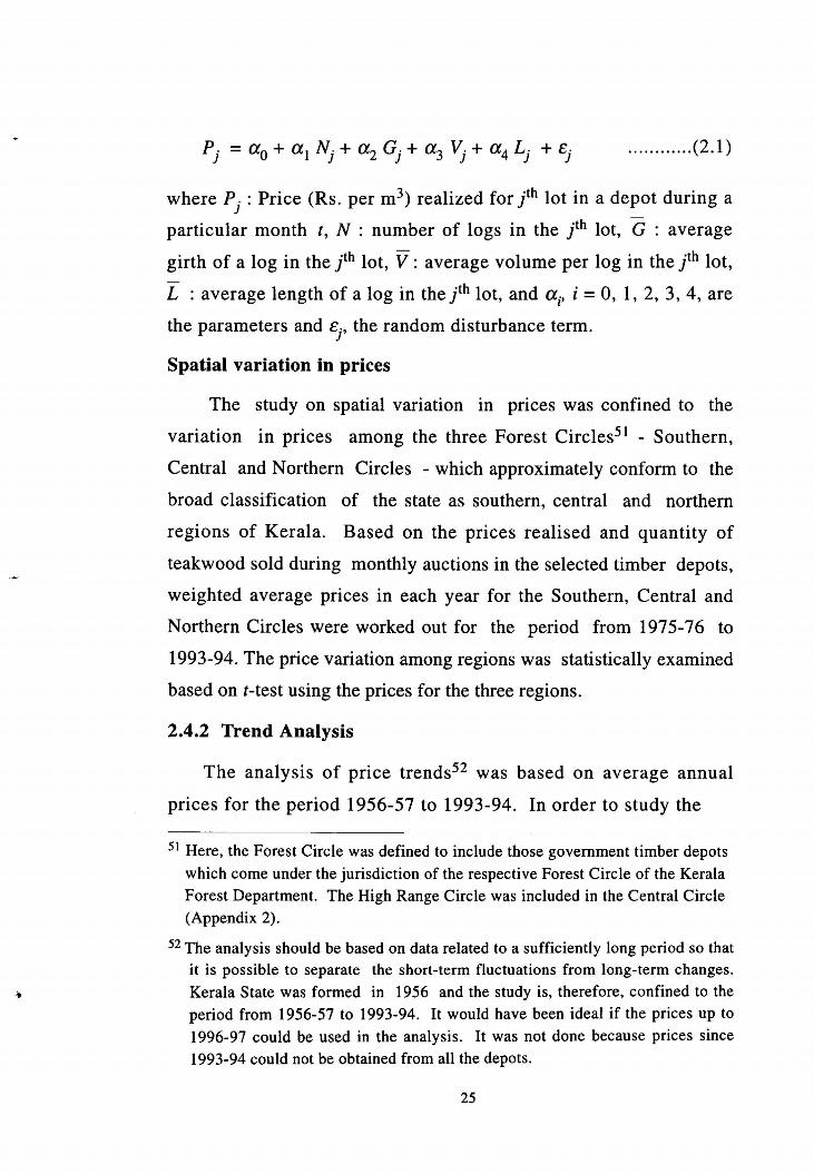
where P, : Price (Rs. per m3) realized for jth lot in a depot during a
particular month t, N : number of logs in the jth lot, 5 : average
girth of a log in the jth lot, V : average volume per log in the jth lot,
: average length of a log in the jth lot, and a , i = 0, 1, 2, 3, 4, are
the parameters and E ~ , the random disturbance term.
Spatial variation in prices
The study on spatial variation in prices was confined to the
variation in prices among the three Forest Circles5' - Southern,
Central and Northern Circles - which approximately conform to the
broad classification of the state as southern, central and northern
regions of Kerala. Based on the prices realised and quantity of
teakwood sold during monthly auctions in the selected timber depots,
weighted average prices in each year for the Southern, Central and
Northern Circles were worked out for the period from 1975-76 to
1993-94. The price variation among regions was statistically examined
based on t-test using the prices for the three regions.
2.4.2 Trend Analysis
The analysis of price trends52 was based on average annual
prices for the period 1956-57 to 1993-94. In order to study the
5 1 Here, the Forest Circle was defined to include those government timber depots which come under the jurisdiction of the respective Forest Circle of the Kerala Forest Department. The High Range Circle was included in the Central Circle (Appendix 2).
52 The analysis should be based on data related to a sufficiently long period so that it is possible to separate the short-term fluctuations from long-term changes. Kerala State was formed in 1956 and the study is, therefore, confined to the period from 1956-57 to 1993-94. It would have been ideal if the prices up to 1996-97 could be used in the analysis. It was not done because prices since 1993-94 could not be obtained from all the depots.
price behaviour of teakwood, it was necessary to examine the price
behaviour of certain important timbers also. Owing to this reason,
seven other important timbers, (i) anjily (Artocarpus hirsutus), (ii)
irul (Xylia xylocarpa), (iii) maruthu (Terminalia paniculata),
( iv) jackwood (Artocarpus heterophyllus), (v) thembavu
(Terminalia crenulata), (vi) venga (Pterocarpus marsupium), and
(vii) venteak (Lagerstroemia microcarpa) were also selected for
the study. The selected timbers including teak accounted for about
48 per cent of the total quantity of timber sold during the period
1956-57 to 1992-93 from all the government depots. The quantum
of disposal of each timber as well as the importance of the timbers
for construction and other common purposes were takwn into
account in the choice of the above seven timbers.
Based on the sale value realised and quantity sold during
monthly auctions, weighted average prices of teak logs in different
girth-classes53 in each year for the state were worked out for the
period from 1975-76 to 1993-94. Girth-classes are based on the
mid-girth of the logs. The different girth-classes are E (logs with
mid-girth 185 cm and above), 1 (150 to 184 cm), 2 (100 to 149
cm), 3 (75 to 99 cm) and 4 (60 to 74 cm). Since the data prior to
1975-76 were not available in most of the depots, the average
prices of teak logs in different girth-classes given in various
Divisional Forest Working Plans were used to fill up the gap in
data. Using the prices and quantity of teak logs sold in different
53 Despite the guidelines for classification of logs (see Appendix l ) , often inter-depot variation is noticed. Further within a class, variation in quality
such as soundness, straightness, etc., are also observed. Since the objective
of the study is to examine the trend in price, quality differences were ignored.
girth-classes, weighted average prices of teakwood (girth-classes
combined) in each year for the period from 1956-57 to 1993-94
were worked out. In a similar manner, average annual prices of
other selected timbers for the period from 1956-57 to 1993-94
were also worked out.
Conversion of current prices to real prices
Changes in the current prices are due to (i) changes in real
prices and (ii) inflation. For eliminating the effect of price change
due to inflation, the current prices are to be deflated with some
price indices54. In this study, the current prices in respect of
various years were deflated with the All India Wholesale Price
Indices of all c o r n m ~ d i t i e s ~ ~ with base year, 1981-82 = 100. This
gave the real prices and this alone reflected the actual change in
prices. The average annual real prices (ie. timber prices at 1981-82
constant prices) of teakwood in different girth-classes for the
period from 1956-57 to 1993-94 were used for analysing the price
trends. The average annual real prices computed for teakwood
(girth-classes combined) and those of selected timbers for the
period from 1956-57 to 1993-94 were used to examine the price
trends of teakwood in comparison with those of selected timbers in
Kerala.
54 Croxton, F. E., Cowden, D. J. and Klein, S. (1973). Applied General Statistics. Parentice-Hall, Inc., Englewood Cliffs, N. J., U.S.A.
55 Government of India (1994). Index number of wholesale prices in India
- Monthly Bulletin for August 1994. Office of the Economic Advisor,
Ministry of Industry, New Delhi.
Trend models and selection criteria
To identify the general trends in prices, moving averages of
average annual real prices were found so as to smoothen out the
effect of year to year fluctuations in prices. Here, 3, 5, and 7 year
moving averages were adopted to explain the general trends.
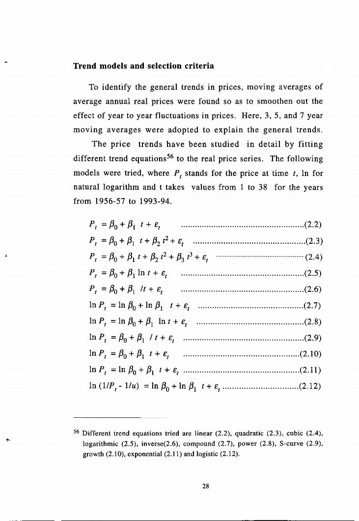
The price trends have been studied in detail by fitting
different trend equations56 to the real price series. The following
models were tried, where P, stands for the price at time t, In for
natural logarithm and t takes values from 1 to 38 for the years
from 1956-57 to 1993-94.
Different trend equations tried are linear (2.2), quadratic (2.3), cubic (2.4),
logarithmic (2.5), inverse(2.6), compound (2.7), power (2.8), S-curve (2.9), growth (2.1 O), exponential (2.1 1) and logistic (2.12).
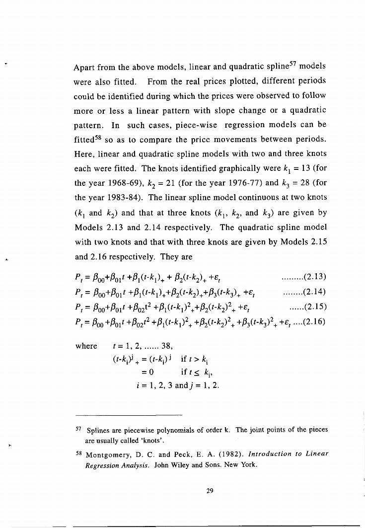
Apart from the above models, linear and quadratic s ~ l i n e ~ ~ models
were also fitted. From the real prices plotted, different periods
could be identified during which the prices were observed to follow
more or less a linear pattern with slope change or a quadratic
pattern. In such cases, piece-wise regression models can be
fitted5* so as to compare the price movements between periods.
Here, linear and quadratic spline models with two and three knots
each were fitted. The knots identified graphically were k l = 13 (for
the year 1968-69), k2 = 21 (for the year 1976-77) and k3 = 28 (for
the year 1983-84). The linear spline model continuous at two knots
(kl and k2) and that at three knots (kl, k2, and k3) are given by
Models 2.13 and 2.14 respectively. The quadratic spline model
with two knots and that with three knots are given by Models 2.15
and 2.16 respectively. They are
where t = 1 , 2 ,...... 38,
( t - k + = ( t ) J if t > k,
= 0 if t 5 k,,
i = l , 2, 3 a n d j = l , 2.
57 Splines are piecewise polynomials of order k. The joint points of the pieces
are usually called 'knots'.
58 Montgomery, D. C . and Peck, E. A . (1982). Introduction to Linear
Regression Analysis. John Wiley and Sons. New York.
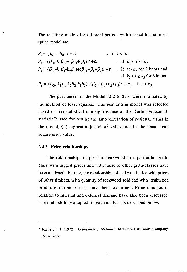
The resulting models for different periods with respect to the linear
spline model are
p, = P00 + 001 t + Et , if t l k,
Pt = (fioo-klPl)+(Pol+ 01) t +Et , if k, c t < k,
P, = (~oo-kl~l-k2~2)+(~ol+~l+~2)t +E, , if t > k2 for 2 knots and
if k, < t 5 k3 for 3 knots
P, = (Poo-klPl-k2P2-k3P3)+(&l+PI+P2+Bs)' +Er. if ' > k3-
The parameters in the Models 2.2 to 2.16 were estimated by
the method of least squares. The best fitting model was selected
based on (i) statistical non-significance of the Durbin-Watson d-
statistic59 used for testing the autocorrelation of residual terms in
the model, (ii) highest adjusted value and iii) the least mean
square error value.
2.4.3 Price relationships
The relationships of price of teakwood in a particular girth-
class with lagged prices and with those of other girth-classes have
been analysed. Further, the relationships of teakwood price with prices
of other timbers, with quantity of teakwood sold and with teakwood
production from forests have been examined. Price changes in
relation to internal and external demand have also been discussed.
The methodology adopted for each analysis is described below.
59Johnston, J . (1972). Econometric Methods. McGraw-Hill Book Company,
New York.
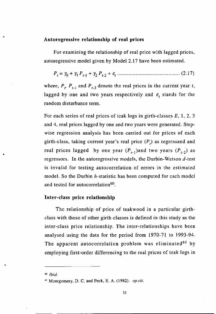
Autoregressive relationship of real prices
For examining the relationship of real price with lagged prices,
autoregressive model given by Model 2.17 have been estimated.
where, P,, P,-1 and denote the real prices in the current year t ,
lagged by one and two years respectively and E, stands for the
random disturbance term.
For each series of real prices of teak logs in girth-classes E, 1, 2, 3
and 4, real prices lagged by one and two years were generated. Step-
wise regression analysis has been carried out for prices of each
girth-class, taking current year's real price (P,) as regressand and
real prices lagged by one year (P,-l)and two years as
regressors. In the autoregressive models, the Durbin-Watson d-test
is invalid for testing autocorrelation of errors in the estimated
model. So the Durbin h-statistic has been computed for each model
and tested for au toc~r re la t ion~~.
Inter-class price relationship
The relationship of price of teakwood in a particular girth-
class with those of other girth-classes is defined in this study as the
inter-class price relationship. The inter-relationships have been
analysed using the data for the period from 1970-71 to 1993-94.
The apparent autocorrelation problem was eliminated61 by
employing first-order differencing to the real prices of teak logs in
Ibid.
Montgomery, D. C. and Peck, E. A. (1982). op.cit.
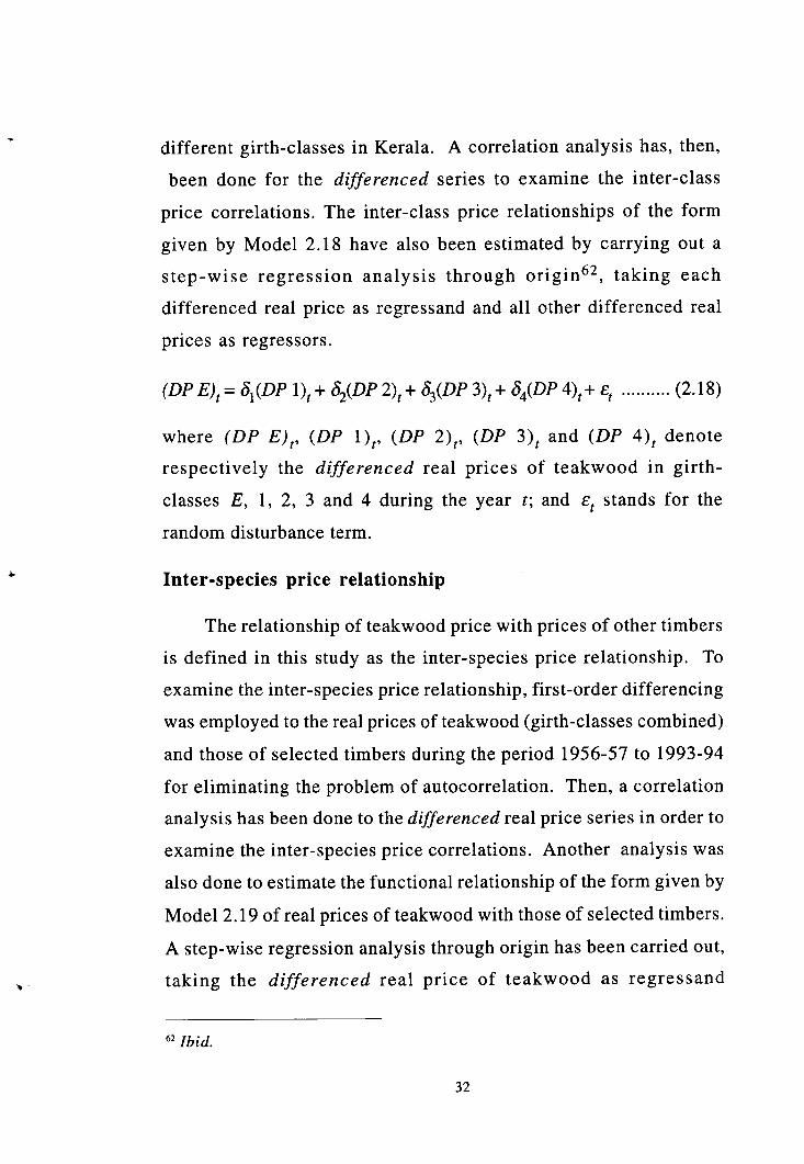
different girth-classes in Kerala. A correlation analysis has, then,
been done for the differenced series to examine the inter-class
price correlations. The inter-class price relationships of the form
given by Model 2.18 have also been estimated by carrying out a
step-wise regression analysis through origin62, taking each
differenced real price as regressand and all other differenced real
prices as regressors.
(DP E), = 4(DP l), + a2(DP 2), + a3(DP 3), + a4(DP 4),+ E, .......... (2.1 8)
where (DP E),, (DP l),, (DP 2),, (DP 3), and (DP 4), denote
respectively the differenced real prices of teakwood in girth-
classes E, 1, 2, 3 and 4 during the year t ; and E, stands for the
random disturbance term.
Inter-species price relationship
The relationship of teakwood price with prices of other timbers
is defined in this study as the inter-species price relationship. To
examine the inter-species price relationship, first-order differencing
was employed to the real prices of teakwood (girth-classes combined)
and those of selected timbers during the period 1956-57 to 1993-94
for eliminating the problem of autocorrelation. Then, a correlation
analysis has been done to the differenced real price series in order to
examine the inter-species price correlations. Another analysis was
also done to estimate the functional relationship of the form given by
Model 2.19 of real prices of teakwood with those of selected timbers.
A step-wise regression analysis through origin has been carried out,
taking the differenced real price of teakwood as regressand
62 Ibid.
and the differenced real prices of selected timbers as regressors.
(DP TE), = ql(DP AN), + q, (DP IR), + q3(DP JA), + q4(DP MAA+
q5 (DP TH), + q6(DP VG), + q,(DP VT), + E, ............................ (2.19)
where (DP TE), (DP AN),, (DP IR),, (DP JA),, (DP MA),, (DP TH),,
(DP VG), and (DP VT), denote the differenced real prices of teak,
anjily, ' i ru l , jack, maruthu, thembavu, venga and venteak
respectively; and E, stands for the random disturbance term.
Price-quantity relationship
For examining the relationship between the real price and total
quantity of teakwood sold, data on total quantity of teakwood sold in
all the government depots together were compiled from the
Administration Reports63 of the Kerala Forest Department for the
period64 from 1956-57 to 1992-93. Autoregressive model of the form
given by Model 2.20 has been estimated, taking real price of teakwood
in the current year (P) as regressand and real price lagged by one
year (P,-,) and quantity of teakwood sold in the current year (Q,) as
regressors.
Price-production relationship
Data on total volume of teakwood produced from forests were
compiled from the Administration Reports of the Kerala Forest
Department for the period from 1956-57 to 1992-93. For examining
63 Kerala Forest Department (1956-57 to 1992-93). Administration Reports. Government of Kerala, Thiruvananthapuram.
64 Data for the year 1993-94 was not available.
the influence of total teakwood p r o d u c t i ~ n ~ ~ from forests on prices,
autoregressive relationship given by Model 2.21 has been estimated,
taking real price of teakwood in the current year (P,) as regressand
and real price lagged by one year (Pt-,), production of teakwood from
forests in the current year (F,) and lagged by one year (F,-,) and two
years (Ft-,) as regressors.
Changes in internal demand
Apart from the fluctuations in timber supply, change in demand
is an important factor that influences the prices. Demand for timber
can be categorised into internal and external demand. Most of the
internal demand for timber is in the construction sector, particularly
in residential buildings and hence the trend in housing and the pattern
of use in the household sector are important factors influencing
demand and consequently the prices. Of the total demand for timber
in Kerala during the year 1987-88, rural household sector accounted
for the major share66. Therefore, it was required to examine the pattern
of timber-use in the rural household sector. The pattern of timber-
use in rural households of Kerala has been examined based on the
65The different sources of teakwood supply in Kerala are home gardens, Kerala
forests and import from other states in India and other countries. The timber
obtained from home-gardens seldom reaches the organised markets and a
major part of it is utilised within the area. Through interview with timber
traders, it has been found that a major part of the imported timber directly goes to industries and the supply through import is dependent on prices prevailing in the retail market rather than prices being determined by the supply. Therefore, in the present study, only the changes in supply (production) of
teakwood from forests including teak plantations alone have been examined. 66 Krishnankutty, C. N. (1990). op.cit.
data available in the survey schedules of the earlier study by the author.
Different species of timbers including teakwood used in house
construction, modification of house by way of addition or repair and
for making furniture, fixtures and implements were included in the
total quantity of timber used in the rural household sector. The
volume of teakwood and other timbers utilised for various uses in the
rural households have been estimated. To get a general picture of the
trend in constructions, over time data on number of residential and
non-residential buildings for the years 1973,1978, 1983, 1988 and
1993 were collected67 from sample panchayats and analysed.
Changes in external demand
Substantial quantities of teakwood and other timbers, both in
round and sawn, are exported to other states, particularly to the wood-
deficit state of Tamil N a d ~ ~ ~ . A large number of traders from Tamil
Nadu also participate in timber auction in the Kerala government
depots. Obviously, auction prices in Kerala are a reflection of the
situation that exists in Tamil Nadu. The quantity of teakwood exported
to other states through the major inter-state forest check-posts at
Kotekar, Vazhikadavu, Walayar, Vaniyampara and Arienkavu were
collected from the registers maintained at the check-posts during the
period from 1980-8 1 to 1993-94. First-order differencing was
employed to the series of real prices of teakwood and quantites of
teakwood exported for eliminating the problem of autocorrelation.
An attempt has been made to estimate the relationship of the
67 The sample Panchayats were Koorkanchery, Vadanappally, Adat and Orumanayur in Thrissur District.
For quite some time, Kerala was net exporter of other timbers. With the decline in the
supply of ordinary construction timbers from Kerala forests, the trend has reversed.
Presently, a large quantity of other timbers such as salwood is imported to Kerala.
form given by Model 2.22 for examining the influence of teakwood-
export on price of teakwood in Kerala.
................................................................ (DP), = K,(DEX)~ + st (2.22)
where (DP), denotes the differenced real price of teakwood (girth-
classes combined) and (DEX), the diferenced quantity of teakwood
exported.
2.4.4 Price Forecasting
For forecasting future prices of teakwood, autoregressive
integrated moving average (ARIMA) model, has been used.69 The
general form of the ARIMA model of order (p,d,q) for a time
series Zt is written as
where $(B) = ( I-$, B-q$ B~-.. .-$~ BP),
0(B) = (1-0, B-O2 ~ ~ - . . . - 0 ~ B4 ),
Zt = Ztj, where B is the backward shift operator,
a, : the random shock which is distributed N(0 , oa2),
d : the degree of differencing.
$(B) and @(B) are called autoregressive operator of order p and
moving average operator of order q respectively. $,, $2,..., $p,
known as autoregressive parameters, and 0,, 02, .... eq known as
moving average parameters, and oa are to be estimated from the
data. When the degree of differencing, d, is zero, Z, is replaced by
5, = 2,- p, where p is the mean of the series 2,. Model 2.23 can
be used for describing stationary and non-stationary time series.
69 BOX, G. E. P. and Jenkins, G. M. (1976). op.cit.
3 6
The method developed by Box and ~ e n k i n s ~ ~ for analysing time
series has four stages -i) identification ii) estimation iii) diagnostic
check and iv) forecasting which are described below.
Identification of the time series model is the determination of
the model. Before establishing a model for a given time series,
whether the given series is stationary or non-stationary has to be
understood. If the frequency of occurrence of autocorrelation of
various lags is very high, it indicates the existence of clear
autocorrelation and the given series is non-stationary. Then, the
non-stationary series should be undergone differencing till the
stationarity state appears and the number of times differencing
sought is the value of d.
The value of p and q are determined as follows. When the
autocorrelation function of the time series is cut off at lag k (where
k>q) and the partial autocorrelation function shows a gradually
declining trend, then the suggested model is MA (q). When the
autocorrelation function shows a gradually declining trend and the
partial autocorrelation function is cut off at p (where k>p), then
the suggested model is AR(p). When both the autocorrelation and
partial autocorrelation functions show a gradual decline, then
ARMA (p, q) model is suggested. If both of them is cut off at q and
p , then it is difficult to determine the model. In this case, three
kinds of models - MA(q), AR(p) and ARMA(p, q) - can be fitted and
later by diagnostic check, the actual model can be determined.
After identifying the model, the parameters in the model are to
be estimated using the maximum likelihood method. After having
estimated the model, the diagnostic check is to be performed. If
70 Ibid.
there exists autocorrelation between the residual terms, the model
is not suitable, otherwise, the model can be accepted. The
autocorrelation of residuals can be tested with Box-Ljung statistic.
If it is non-significant, there is no autocorrelation. After checking
the model for Box-Ljung statistic, the best model among the
different models identified can be selected based on (i) the least
values of Akaike Information Criterion (AIC) and Schwartz
Bayesian Criterion (SBC), (ii) relatively small residual standard
error, ( i i i ) low mean absolute prediction error and (iv)
comparatively small number of parameters.
The method developed by Box and Jenkins described above has
been adopted for analysing the time series of teakwood prices. The
average annual current prices of teakwood in girth-classes 1, 2 and
3 for the 53 year period from 1941-42 to 1993-94 in ICerala71 were
used for ARIMA modelling and thereby forecasting future prices.
The data for the period from 1941 -42 to 1955-56 was compiled from various Divisional Forest Working Plans in Travancore and Cochin States and Malabar District (Madras Presidency) which constitute the present Kerala State.