lith-isy-ex--10/4270--se linköping 2010 · loads. in order to prevent the draining of blood from...

Institutionen för systemteknik

Department of Electrical Engineering

Examensarbete

Pressure Monitoring and Fault Detection of an Anti-g Protection System

Examensarbete utfört i Fordonssystem vid Tekniska högskolan i Linköping

av

Kim Andersson

LITH-ISY-EX--10/4270--SE Linköping 2010

Department of Electrical Engineering Linköpings Tekniska Högskola Linköping University Institutionen för systemteknik S-581 83 Linköping, Sweden 581 83 Linköping

3

Pressure Monitoring and Fault Detection of an Anti-g Protection System

Examensarbete utfört i Fordonssystem vid Tekniska högskolan i Linköping

av

Kim Andersson

LITH-ISY-EX--10/4270--SE Linköping 2010

Handledare: Emil Larsson ISY, Linköpings universitet Fredrik Fisk Saab AB Markus Klein Saab AB Examinator: Erik Frisk ISY, Linköpings universitet

Linköping, 5 maj, 2010

Presentationsdatum 2010-05-05 Publiceringsdatum (elektronisk version) 2010-05-12

Institution och avdelning Institutionen för systemteknik Department of Electrical Engineering

URL för elektronisk version http://urn.kb.se/resolve?urn=urn:nbn:se:liu:diva-56286

Titel Title Pressure Monitoring and Fault Detection of an Anti-g Protection System Författare Author Kim Andersson

Sammanfattning Abstract

When flying a fighter aircraft such as the JAS 39 Gripen, the pilot is exposed to high g-loads. In order to prevent the draining of blood from the brain during this stress an anti-g protection system is used. The system consists of a pair of trousers, called the anti-g trousers, with inflatable bladders. The bladders are filled with air, pressing tightly on to the legs in order to prevent the blood from leaving the upper part of the body.

The purpose of this thesis is to detect if the pressure of the anti-g trousers is deviating from the desired value. This is done by developing a detection algorithm which gives two kinds of alarm. One is given during minor deviations using a CUSUM test, and one is given at grave deviations, based on different conditions including residual, derivative and time. The thresholds, in which between the pressure should lie in a faultless system, are calculated from the gload value. The thresholds are based upon given static guidelines for the pressure tolerance area and are modified in order to adapt to the estimated dynamics of the system.

The values of the input signals, pressure and g-load, were taken from real flight sessions. The validation has been performed using both faultless and faulty flight sequences, with low false alarm rate and no missed detections. All together the detection system is considered to work well.

Nyckelord EWMA, JAS 39 Gripen, Anti-g system, Fault detection, CUSUM

Språk Svenska X Annat (ange nedan) Engelska Antal sidor 88

Typ av publikation Licentiatavhandling X Examensarbete C-uppsats D-uppsats Rapport Annat (ange nedan)

ISBN (licentiatavhandling) ISRN LITH-ISY-EX--10/4270--SE

Serietitel (licentiatavhandling) Serienummer/ISSN (licentiatavhandling)

7

Abstract When flying a fighter aircraft such as the JAS 39 Gripen, the pilot is exposed to high g-loads. In order to prevent the draining of blood from the brain during this stress an anti-g protection system is used. The system consists of a pair of trousers, called the anti-g trousers, with inflatable bladders. The bladders are filled with air, pressing tightly on to the legs in order to prevent the blood from leaving the upper part of the body. The purpose of this thesis is to detect if the pressure of the anti-g trousers is deviating from the desired value. This is done by developing a detection algorithm which gives two kinds of alarm. One is given during minor deviations using a CUSUM test, and one is given at grave deviations, based on different conditions including residual, derivative and time. The thresholds, in which between the pressure should lie in a faultless system, are calculated from the g-load value. The thresholds are based upon given static guidelines for the pressure tolerance area and are modified in order to adapt to the estimated dynamics of the system. The values of the input signals, pressure and g-load, were taken from real flight sessions. The validation has been performed using both faultless and faulty flight sequences, with low false alarm rate and no missed detections. All together the detection system is considered to work well. Sammanfattning När en pilot flyger ett stridsflygplan så som JAS 39 Gripen, så utsätts denne för höga g-laster. För att förhindra ett blodtryckfall i hjärnan under denna påfrestning används ett anti-g-skyddssystem, bestående av ett par byxor med luftblåsor, ett par s.k. anti-g-byxor. Blåsorna fylls med luft och spänns åt runt benen för att förhindra att blodet lämnar överkroppen. Syftet med detta examensarbete är att detektera om trycket i anti-g-byxorna avviker från börvärdet. Detta görs genom att utveckla en detektionsalgoritm som ger två larmtyper. Ett ges vid mindre avvikelser, baserat på ett CUSUM-test, och ett ges vid allvarligare avvikelser, baserat på olika kriterier, däribland residual, derivata och tid. Trösklarna som trycket bör ligga innanför vid ett felfritt system beräknas utifrån g-lasten. Trösklarna är baserade på givna statiska riktlinjer för tryckets toleransområde och modifieras för att anpassa dem till den skattade dynamiken i systemet. Insignalerna, d.v.s. tryck och g-last, är tagna från verkliga flygpass. Valideringen av algoritmen är gjord på data från både felfria pass och pass med fel, med låg andel falsklarm och inga missade detektioner. Överlag anses detektionssystemet fungera bra.

9

Acknowledgements I would like to thank my examiner, Erik Frisk, who introduced me to and guided me through this master thesis, my supervisor at Linköping University, Emil Larsson, for all good feedback and suggestions, my supervisors at Saab AB, Fredrik Fisk, for many good discussions and helpful information about the anti-g-system, Gripen and the life at Saab, and Markus Klein, who gave me valuable feedback and support and who constantly pushed me in the right direction, Ylva Nilsson, for lending me several of her books and for helpful suggestions, and finally my colleagues at TDGA, for their support, all tasty cakes and enjoyable coffee and lunch breaks.

Kim Andersson

Linköping, April 2010

11

Contents 1 Introduction ............................................................................................ 13

1.1 Background..................................................................................... 13 1.2 Problem and conditions................................................................... 13 1.3 Purpose and Goals........................................................................... 14 1.4 Thesis outline.................................................................................. 14

2 System description and flight data........................................................... 17 2.1 The OBOG & Anti-g system........................................................... 17 2.2 The anti-g trousers .......................................................................... 17 2.3 The PSU ......................................................................................... 18 2.4 Flight data....................................................................................... 19

2.4.1 Flight modes............................................................................ 20 2.5 Signal processing of measurement data ........................................... 22

2.5.1 RMSE, NRMSE...................................................................... 23 2.5.2 Choice of -parameter........................................................... 23

2.6 The static thresholds........................................................................ 23 2.7 The earlier attempt .......................................................................... 24

2.7.1 The model ............................................................................... 25 2.7.2 The thresholds ......................................................................... 25 2.7.3 Simulation and verification...................................................... 25

3 Adapting the thresholds .......................................................................... 27 3.1 Introduction .................................................................................... 27 3.2 System approximation – first order.................................................. 28

3.2.1 Higher system order ................................................................ 29 3.3 Estimation of a -parameter ............................................................. 29

3.3.1 Estimation result...................................................................... 31 3.4 Adaptive filtering of the thresholds ................................................. 31

3.4.1 Estimating derivative............................................................... 33 3.4.2 Special solution: slow deflation ............................................... 34 3.4.3 The Adapted Thresholds Algorithm......................................... 34 3.4.4 The filter modes ...................................................................... 36

3.5 The result from adapting the thresholds........................................... 38 4 Detection system .................................................................................... 41

4.1 Introduction .................................................................................... 41 4.1.1 The purpose of the maintenance alarm..................................... 41 4.1.2 The purpose of the acute alarm................................................ 42

4.2 Maintenance alarm.......................................................................... 42 4.2.1 CUSUM test............................................................................ 42

4.3 Acute alarm .................................................................................... 44 4.3.1 Residual alarm......................................................................... 45 4.3.2 Derivative alarm...................................................................... 48 4.3.3 Time alarm.............................................................................. 49 4.3.4 All alarms flags set before acute alarm .................................... 51 4.3.5 Acute alarm at low g-load........................................................ 54 4.3.6 Maintenance alarms becomes acute ......................................... 55

12

4.3.7 Acute alarm using CUSUM-test (alternative solution) ............. 55 4.4 The detection system at safety pressure (level flight)....................... 56

4.4.1 Acute alarm when safety pressure is too low ........................... 57 4.5 Main differences from the earlier attempt........................................ 57

5 Experiments and results .......................................................................... 60 5.1 Data and conditions for the results................................................... 60 5.2 Test using training data ................................................................... 60

5.2.1 Test result................................................................................ 61 5.3 Test using unknown data................................................................. 62

5.3.1 Test result................................................................................ 63 5.4 Evaluation of different alarm situations ........................................... 64

5.4.1 Maintenance alarm: depression................................................ 64 5.4.2 Maintenance alarm: overpressure ............................................ 65 5.4.3 Acute alarm: maintenance alarms become acute ...................... 66 5.4.4 Acute alarm: no/slow pressure build-up................................... 67 5.4.5 Acute alarm: pressure drop...................................................... 68 5.4.6 Acute alarm: fluctuating depression......................................... 69 5.4.7 Acute alarm: Safety pressure lost (simulation) ......................... 70

5.5 Noise sensitivity.............................................................................. 71 5.6 Maintenance false alarms risk due to the adapted thresholds............ 74

6 Summary and future work....................................................................... 76 6.1 Summary ........................................................................................ 76 6.2 Future work/Alternative solutions ................................................... 76

Nomenclature ................................................................................................. 80 References...................................................................................................... 82 Appendix A: Adaptive filtering of the thresholds using Test mode ................. 84

13

1 Introduction In this first chapter an introduction to this thesis will be given. The background, purpose and goal of the thesis are explained, and a brief outline of the chapters to follow is given.

1.1 Background Saab AB is a global company, with 13300 employees all over the world [9]. The company was founded 1937, with operations in several countries worldwide. Saab AB is active in many different areas, including both civil and military. The most famous product at Saab AB is the fighter aircraft JAS 39 Gripen. This master thesis was performed at Saab Aerosystems, at the Department of Escape & Oxygen System. When flying a fighter aircraft such as the JAS 39 Gripen, the pilot is exposed to high g-loads. In order to prevent the draining of blood from the brain during this stress an anti-g protection system is used. The system consists of a pair of trousers, called the anti-g trousers, with inflatable bladders. The bladders are filled with air, pressing tightly on to the legs in order to prevent the blood from leaving the upper part of the body. The feed air and hence the pressure of the anti-g trousers is in JAS 39 Gripen controlled by a unit called the PSU (Pilot Service Unit), described in chapter 2. The pressure of the anti-g trousers is referred to as the anti-g pressure. In the nineteen-nineties an attempt was made to create a detection system for faulty anti-g pressure. The developed system was tested in simulations and was considered to work well, although real flight tests resulted in false alarms. A few suggestions of improve were made, but the project were canceled until further advice. The false alarm risk made it difficult to trust the system. The earlier attempt is described in chapter 2.7.

1.2 Problem and conditions The anti-g protection system is a single point system, i.e., there is no back-up system. Therefore there is a need of anti-g pressure monitoring and fault detection in order to improve flight safety. Presently no such detection system exists in JAS 39 Gripen. The pressure is subjectively judged by the pilot, which have resulted in returned PSU:s where no faults have been found. Hence, fault detection of the pressure will be a safety to the pilot as well as an indication whether the system functions properly or not. It can however be difficult to send an alarm to the pilot fast enough, since the draining of blood from the brain can be very quick when loosing the anti-g pressure during high g-loads.

14

Several measurements of the anti-g pressure have been made during real flight test, and this thesis is based upon these measurements. The sensors are in this thesis considered to be faultless, even though faults normally can occur. There are also given guidelines for the tolerance area of the anti-g pressure which will be used in the thesis.

1.3 Purpose and Goals The purpose and goal of this thesis is to detect a defect anti-g protection system, i.e., detect if the pressure of the anti-g trousers is deviating from the desired value. The source to the fault will not be identified. The developed algorithm shall consist of:

A detection system, detecting faulty anti-g pressure Two kinds of alarm; maintenance alarm and acute alarm

The maintenance alarm will be given in situations when the anti-g pressure is deviating from the desired in an alarming way, but is of no immediate danger. The alarm shall not restrain the pilot or the mission, but generate a failure report after flight. The acute alarm will be given directly to the pilot in situations when a faulty anti-g pressure indicates an immediate danger. The detection system must also, as far as possible, avoid false alarms; hence the pilot might loose confidence in the system.

1.4 Thesis outline The chapters of this thesis will have the following outline: Chapter 2 This chapter includes a brief description of the anti-g

protection system. The measurement data and the guidelines of the anti-g pressure tolerance area are presented. The former attempt to develop a detection system is described. The chapter also includes signal processing of the measurement data.

Chapter 3 This chapter describes the adaption and modification of the

anti-g pressure tolerance area, which will be used as thresholds in the detection system algorithm.

Chapter 4 This chapter describes the detection system algorithm. Chapter 5 This chapter discusses and presents the obtained results of

the detection system experiments and verification.

15

Chapter 6 This chapter presents a summary of the thesis and includes a suggestion of future works.

17

2 System description and flight data In this chapter a background of the system is given, including a brief description of the units involved. Also the measurement data provided for this thesis is described and how the data sequences are interpreted. The threshold guidelines used in the detection system are presented. The chapter ends with a comprehensive description of the earlier attempt to develop a detection system.

2.1 The OBOG & Anti-g system In Figure 1 a comprehensive view of the OBOG (Onboard Oxygen Generator) & Anti-g system can be seen. The ECS (Environmental Control System) provides the system with temperature and pressure controlled bleed air. Two pressure transducers, named 15HC and 17HC in the figure, are used to monitor the supply pressure to the OBOG & Anti-g system. From the OBOG unit, oxygen enriched breathing gas is created and sent on to a breathing regulator which is a part of a unit called the PSU (Pilot Service Unit). The anti-g bleed supply is fed through a PRV (Pressure Regulating Valve), a RV (Relief Valve) and a WDV (Water Drain Valve) before reaching the PSU. The AIU (Aircraft Interface Unit) monitors some functions of the system, such as BEOS (Back-up & Emergency Oxygen Supply) gas pressure, continuous high breathing gas flow, and on/off signals from BEOS and the PSU. It also receives warnings from the OBOG unit and monitors the pressure sensors 15HC and 17HC. The AIU also have the function to automatically select BEOS instead of OBOG breathing gas.

2.2 The anti-g trousers The anti-g trousers consists of a pair of tightly-fitted trousers with inflatable bladders. When filled with air the trousers will rapidly press on the legs to restrict the draining of blood from the brain during high g-loads. This pressure will be referred to as the anti-g pressure and is the pressure which will be supervised in this thesis. The trousers are connected by a hose to the PSU (Pilot Service Unit), attached to the ejection seat.

18

Figure 1. A comprehensive view of the OBOG & Anti-g system.

2.3 The PSU The PSU is an entirely pneumatic and mechanical unit. It controls the anti-g pressure, as well as the pilot’s breathing gas which is provided by the OBOG unit. The air is fed through the PSU and sent to the trousers. The trousers will always be filled with a basic amount of air, called the safety pressure. The safety pressure is needed to make sure full protection is available at a sudden increase of g-load. The PSU contains an anti-g valve that pneumatically and mechanically controls the air supply of air pressure to the anti-g trousers. The pressure given from the PSU is directly related to the level of g-load [10]. A schematic view of the PSU can be seen in Figure 2.

19

Figure 2. A schematic view of the PSU unit.

2.4 Flight data The data in this thesis is provided from Saab AB. The data comes from several different flight occasions and different PSU:s, about thirty individuals. The measured signals are the anti-g pressure mp and the g-load mg . The anti-g pressure has been measured with a sensor placed inside the anti-g trousers, and the g-load was measured at the pilot’s seat. A typical flight sequence from a faultless flight can be seen in Figure 3. It contains several turns of different kinds. A turn is a greater change in g-load, which in the figures is shown as changes in pressure. The units and scale of the figures in this thesis is not presented due to avoiding giving the air craft performance away.

20

2.4.1 Flight modes In order to explain what happens during a flight sequence, it can be divided into smaller sequences, in this thesis called flight modes. Examples of the flight modes are shown in Figure 3.

Figure 3. Example of a whole flight sequence, showing the sequences level flight, curve and swaying.

Level flight When flying straight forward the anti-g trousers contains a safety pressure, close to constant, see Figure 4. The changes in g-load at that time are very small. The jagged appearance is a result of the A/D-converter resolution. Curve and swaying A flight sequence contains many turns. The appearance of a single turn with high g-load can be seen in Figure 5 and will in this thesis be referred to as a curve. A sequence with several smaller turns, i.e., turns with lower g-loads, close after each other during a longer time period will be referred to as swaying, see Figure 6.

21

Figure 4. Sequence from flying straight forward, i.e., level flight.

Figure 5. A single turn during high g-load, referred to as a curve sequence.

22

Figure 6. Several smaller turns during lower g-load close after each other, referred to as sway sequence.

2.5 Signal processing of measurement data In order to reduce noise in the signals from the provided measurement data, i.e., g-load and anti-g pressure, the signals are filtered through a low-pass filter. In this thesis the filter is an exponentially weighted moving average (EWMA) filter [1]:

10,)()1()()( 1 kkk tutyty (2.1)

where )( kty is the filter output signal and )( ktu is the filter input signal at a certain time kt . The parameter is also called the forgetting factor [2]. The quotient )1(1 represents the number of old samples that are remembered during the filter process, although since the filter is exponentially weighted, the latest samples are higher weighted [3]. The filter parameter can also be calculated as

sT (2.2)

where sT is the sample period and is the time constant of the filter.

23

2.5.1 RMSE, NRMSE To evaluate how well the filter works, a comparison of the low-pass filtered signal )( kty and the un-filtered signal )( ktu is done in order to see how large the deviation is. This is done using Root Mean Square Error (RMSE) [2]:

1

0

2))()((1 N

iikik tytu

NRMSE (2.3)

Normalized RMSE (NRMSE) shows the deviation in percentages:

%100minmax uu

RMSENRMSE (2.4)

where the RMSE is divided by the range of observed values.

2.5.2 Choice of -parameter If the -value is close to 1, the time constant of the filter will be large and more samples will be remembered. Hence the filtered signal will be smoother, but also react slower to quick changes in the input signal. A smaller -value gives a smaller time constant, and an output signal that follows the input signal quicker. A noisy input signal would thereby give a noisy output signal. In this thesis the ad hoc chosen -parameter is a compromise from what is described above. It is important that the filtered signal does not respond too slowly to quick changes in the input signal, since it will cause a delay in all decisions based on this signal. It is also desired to remove noisy parts in the input signal, and hence the -parameter should not be too small. The chosen

-value is also considered to be an -value which corresponds to an accepted delay in the filtered signal, i.e., the number of samples being remembered. The chosen -parameter corresponds to approximately 7 samples.

2.6 The static thresholds There are certain guidelines to what anti-g pressure value a specific g-load value should give. These guidelines are based on medical research and recommendations [11]. At low g-loads the anti-g trousers should have a constant safety pressure, and above a certain g-load the pressure should increase linear to the g-load. However, the pressure should never exceed a certain level, and should therefore be constant at very high g-loads.

24

Figure 7 shows the tolerance zone for the anti-g pressure as a function of g-load. The upper and lower lines will in this thesis be referred to as the upper and lower static threshold, max,sl and min,sl . The thresholds can be described as:

max

maxmin

min

max

min

,gg

ggggg

Kmgk

Kls (2.5)

where the constants minK , maxK , ming , maxg , k and m have different values for the upper and lower thresholds.

Figure 7. The static thresholds as a linear function of the g-load.

The areas at low respectively high g-load in Figure 7 where the static thresholds are constant will in this thesis be referred to as the lower and higher saturated zone respectively.

2.7 The earlier attempt In the former attempt to create a detection system for faulty anti-g pressure two input data were used; the anti-g pressure measured inside the anti-g trousers, and the g-load zN , measured at the center of gravity of the plane. That is, the g-load was not measured at the pilot’s seat. Hence a model describing the g-load perceived by the PSU, and the anti-g pressure this g-load should give rise to, was needed. The exact procedure of how this model was estimated was not described or found.

25

2.7.1 The model The model developed to describe the anti-g pressure included a fixed time delay, to compensate for the difference in g-load at the pilot’s seat and the center of gravity of the plane. In other words, the measured value zN was delayed a certain time and was referred to as dN . The model also included a low-pass filter describing the dynamics of the PSU. The fixed time delay and the parameter value of the low-pass filter were then combined into a new low-pass filter, with the measured g-load zN as input signal and a filtered g-load value, filtN , as output signal.

2.7.2 The thresholds Three g-load values were used to calculate the upper and lower thresholds for the measured anti-g pressure; the filtered g-load filtN , the delayed g-load dN , and the measured g-load zN . If af is the upper threshold function and bf is the lower threshold function, then they were determined as:

)),,(max( valuesholdLower thre

)),,(min( valuesholdUpper thre

filtdzb

filtdza

NNNfNNNf

(2.6)

Just as in this thesis the static thresholds described in chapter 2.6 and (2.5) were used as a guideline to estimate these thresholds. An alarm was given whenever the measured anti-g pressure exceeded the thresholds [12].

2.7.3 Simulation and verification A simulation of the model was done in SYSIM, which is a simulation tool developed by Saab AB. The input data to the simulation was taken from centrifugal tests and measurements from the PSU system contractor, i.e., the data did not come from actual flight tests. Several fault modes were simulated, as well as faultless ones, and the result was approved. The sample frequency of the data was about a third of the sample frequency of the data provided for this thesis. Verification was also done by testing the model in real flight tests. However, during flight several alarms were given from the detection system for no apparent reason. Troubleshooting afterwards gave no obvious reasons to why the thresholds were exceeded at the alarm time points. It did however occur more often in the borderline between the saturated zones and the variable zone of the static

26

thresholds, see chapter 2.6. Also, manual test of the PSU function resulted in false alarm. Manual tests can be done by the pilot by pressing a button that feed air into the trousers up to a certain pressure level, followed by a quick deflation. The manual test during the flight tests was interpreted by the detection system test as a great overpressure, resulting in a false alarm [13]. Suggestions were made to improve the detection system, but the project was canceled until further advice [14]. The false alarm risk made it difficult to trust the system.

27

3 Adapting the thresholds This chapter describes the thresholds which will be used by the detection system and how they are determined. This includes a system approximation in order to estimate the dynamics of the PSU unit, from which the thresholds will be emanated.

3.1 Introduction The PSU combined with the anti-g trousers has a certain dynamic behavior, i.e., it takes time to inflate and deflate the anti-g trousers when there is a change in g-load. This dynamic will be referred to as the PSU dynamic, but describes the combined dynamics of the PSU and anti-g trousers. The static thresholds are calculated as a direct function of g-load and hence the PSU dynamics are not taken into consideration. When there are rapid changes in g-load, the pressure might end up outside one of the thresholds for a while which results in false alarms, see Figure 8. Hence, before a diagnosis statement is made, the thresholds should be adapted to follow the dynamics of the PSU. This only needs to be done for the static thresholds between the saturated zones described in chapter 2.6. The adapted and static thresholds will be the same in the saturated zones. All data used in the figures in this chapter are from faultless PSU:s.

Figure 8. The anti-g pressure (solid line) ends up outside the allowed area between the static thresholds (dashed lines).

28

3.2 System approximation – first order To get a hint of the system behavior, a comparison is made between the filtered pressure fp and the desired pressure, i.e., the pressure that is expected at a certain g-load-value. The desired pressure, in this thesis called the reference pressure, refp , is calculated as the mean value of the upper and lower static thresholds, see (2.5):

highprefkf

highprefkflowpref

lowprefkf

highref

kf

lowref

kref

gtggtgg

gtg

pdtgc

ptp

,

,,

,

,

,

)()(

)(,)()( (3.1)

The reference pressure as the mean value of the static thresholds in chapter 2.6, Figure 7, is illustrated in Figure 9.

Figure 9. The reference pressure (middle dashed line) as the mean value of the static thresholds, all three are linear functions of the g-load.

Figure 10 shows the relation between refp and fp .

29

Figure 10. The relation between the desired (reference) pressure and the anti-g pressure.

The delay of the output signal reminds of a first order system, i.e., the filtered pressure can be approximated as the first order low-pass filtered reference pressure. As a first approach, the system can therefore be described with the EWMA-filter, see chapter 2.5:

)()1()()( 1 krefkfkf tpatpatp (3.2) Estimation of the a -parameter is described in chapter 3.3.

3.2.1 Higher system order In this thesis the first order approximation of the system is considered to be enough, and no further estimation of system order will be done. However, it is probable that the PSU is a system of higher order, and future investigation can therefore be of interest, see chapter 6.2.

3.3 Estimation of a -parameter Filtering of the static thresholds through a first order low-pass filter will give them a similar dynamic behavior as the measured pressure. The filter used in this thesis is the EWMA-filter:

)()1()()( 1 kkk tuatayty (3.3)

30

where y is the output signal and u is the input signal to the filter. Note that this a -parameter is not the same parameter as the -parameter used in the low-pass filter process of the measurement data in chapter 2.5. The -parameter is chosen ad hoc in order to reduce noise while the a -parameter in this chapter is estimated in order to describe the dynamics. The a -parameter is estimated using linear regression [6]. The filter can be written as:

)()( kk tatY (3.4) where

)()()()(

)()()()(

)(,

)()()()(

)()()()(

)(

1

12

21

10

11

22

11

NN

NN

k

NN

NN

k

tutytuty

tutytuty

t

tutytuty

tutytuty

tY (3.5)

and 00 )( yty . The estimation is done for several different flying events and flight modes, i.e., whole sequence, curve and swaying, see chapter 2.4. The flight mode level flight will not be used in the estimation since the sequences almost solely occur in the lower saturated zone, see chapter 2.6. The time of climb varies between different pressure areas. For example, inflating the trousers works somewhat slower when they only contain safety pressure. Deflating the trousers also works a bit slower at low pressures. Therefore two estimations are made; high a and low a , i.e., above respectively below a certain pressure level. Differences in time of climb between the PSU individuals requires the estimation to be made for the PSU with the largest accepted time constant, in order to find a filter which can operate on every individual. Therefore the a -parameter is chosen to be slightly larger than these estimation results. From (2.2) the relation between the a -parameter and the time constant is given as:

aaTs

1 (3.6)

31

3.3.1 Estimation result The reference pressure filtered through (3.3) with the two different estimations of the a -parameter can be seen in Figure 11. The result is compared to the measured anti- pressure. The dotted line shows the result when using the high a at all g-loads and the dash-dotted line is the result from using the low a at all g-loads. The dashed line shows the result when using low a at low g-loads and high a at high g-loads.

Figure 11. Filtered reference pressure using the two estimated a-parameters, low a (dash-dotted line) and high a (dotted line), and the combination of the two (dashed line).

When only using the high a the output signal follows the anti-g pressure well, except for at the beginning of the curve, where the signal increases too early. Here the output signal from using the low a follows better, but it is too slow at higher g-loads. At the deflation at end of the curve the output signal from using the high a still follows the anti-g pressure well. However, the output signal from using the combined a -parameters is preferred in situations when the deflation of the trousers is slower than in this example. Hence using different a -parameters at low respectively high g-loads gives a better estimation of the PSU dynamics.

3.4 Adaptive filtering of the thresholds Low-pass filtering of the static thresholds creates a certain delay in the threshold output signal, and hence a change of threshold value. This change is only desired when it is not inflicting on the allowed pressure area between the static thresholds. For example, filtering the upper threshold while the g-load increases,

32

will result in a threshold value that is lower than the static threshold value, and can also risk false alarms. Therefore low-pass filtering of the upper threshold should only occur when the g-load decreases where it will follow the behavior of the anti-g pressure signal. The risk when low-pass filtering the upper threshold without taking this into consideration is shown in Figure 12, where the filtered threshold is referred to as none-adapted. Likewise the lower threshold should only be filtered when the g-load increases where it will follow the anti-g pressure signal behavior. Otherwise the low-pass filtered threshold, i.e., the lower none-adapted filtered threshold, can result in a higher value than the static threshold value and even risk false alarms, see Figure 13. Derivative estimation of the reference pressure, i.e., indirectly the derivative of the g-load, can be used to decide when to filter the static thresholds. New dynamic thresholds will then be made from a combination of the original and filtered static thresholds.

Figure 12. The upper none-adapted low-pass filtered threshold and the upper static threshold with the anti-g pressure. The none-adapted upper threshold is lower than the static one when the g-load increases, and therefore restrains the allowed pressure area and even risks false alarms. Still, it has the desired behavior when the g-load decreases, where the deflation delay otherwise will risk false alarms.

33

Figure 13. The lower none-adapted low-pass filtered threshold and the lower static threshold with the anti-g pressure. The none-adapted lower threshold is higher than the static one when the g-load decreases, and therefore restrains the allowed pressure area and even risks false alarms. Still, it has the desired behavior when the g-load increases, where the inflation delay otherwise will risk false alarm.

3.4.1 Estimating derivative The derivative approximation method used in this thesis is the finite difference approximation method [5], which here can be described as

1

1)()()()(

kk

krefkrefkrefkref tt

tptpdt

tdptp (3.7)

where 1kk tt is the time between two samples, i.e., the sample period sT . refp is the reference pressure, see chapter 3.2. In order to avoid noise in the derivative signal, a simple moving average filter is used:

Nktp

NkT

tptpN

Ttptp

Ntp

kref

s

Nkrefkref

k

Nkn s

nrefnrefkref

,0)(

,)()(1

)()(1)(1

1

(3.8)

where N is the number of samples used in the average filter.

34

The derivative is always zero in the saturated zones described in chapter 2.6, since the reference pressure is constant, see (3.1). In this thesis the derivative will also considered to be zero outside the saturated zones if the derivative value is very small, i.e., refp , where is a small number close to zero.

3.4.2 Special solution: slow deflation The static thresholds should not be filtered when the derivative of the reference pressure is considered to be zero, since the reference pressure then is constant. Low-pass filtering the lower static threshold only when the g-load increases, and the upper one only when the g-load decreases, and not otherwise, is enough in most cases. However, there is one situation that needs further handling. Slow deflation refers to the deflation of the trousers at the end of a turn, just before the anti-g pressure returns to safety pressure. The g-load is low and the deflation takes longer time because of the already low pressure. This situation requires the upper threshold to be filtered some time after the reference pressure has entered the saturated zone, where 0refp , otherwise there is a risk of false alarm, see Figure 14.

Figure 14. The upper adapted threshold shifts to the static threshold when entering the saturated zone. The slow deflation causes an unnecessary alarm.

3.4.3 The Adapted Thresholds Algorithm A basic principle of how the adapted threshold algorithm works is shown in Figure 15. Input values to the algorithm are the derivative of the reference

35

pressure, refp , and the upper and lower static threshold values, max,sl and min,sl , described in chapter 2.6. The output values are the values of the new adapted upper and lower thresholds, max,al and min,al . In this filter algorithm only the sign of the derivative is of interest and the filtering decisions are based on the two latest derivative signs. Increasing g-load gives a derivative which is positive, while decreasing g-load gives a negative derivative. The algorithm contains several filter modes based on the derivative signs. These are positive mode, negative mode, slow deflation mode and zero mode. There is also a solution of how to handle two derivatives of different signs. Chapter 3.4.4 gives a further description of these modes. Using two samples of derivative signs instead of just one gives more certain estimation of which filter mode the algorithm should enter. It is also easier to detect changes in the derivative sign. Since the derivative value is the average value from a few of the latest samples, the contribution of using more than two derivative samples to the algorithm is negligible. The filter process is done for every sample, and is constructed so that the area between the adapted thresholds never inflicts the area between the static thresholds. In other words, if the adapted thresholds created in these filter modes restrains the allowed pressure area between the static thresholds, then the inflicting threshold will be set to the static threshold instead.

36

Figure 15. Schematic view of the Adapted Thresholds Algorithm.

3.4.4 The filter modes Positive and Negative mode If the two latest derivative samples are positive, the algorithm enters Positive mode. The lower adapted threshold is set to the filtered lower static threshold, while the upper adapted one is set to the original static threshold. If the

37

derivatives are negative the algorithm enters Negative mode. Then the upper adapted threshold is set to the filtered upper static threshold, while the lower one is set to the original static threshold. The filter initial value, )( 1kty in (3.3), is either the previous adapted threshold value )( 1maxmin/, ka tl . The two modes can be seen in Figure 16. In Negative mode a flag called the deflation flag is set. This is done in order to prepare for the Slow Deflation mode, see description below.

Figure 16. Schematic view of Positive (to the left) and Negative (to the right) mode. In Negative mode the deflation flag is set in order to prepare for Slow Deflation Mode.

Slow Deflation mode The need of Slow Deflation mode is described in chapter 3.4.2. The algorithm enters this mode when the derivative goes from being negative, i.e., goes from Negative mode, to being zero. If the following derivatives remains zero there is a risk of slow deflation, and therefore the upper threshold must continue to be filtered for a certain time period, called the deflation period, chosen in advance. The algorithm will enter the Slow Deflation mode as long as the derivative stays zero and the deflation flag is set. If the algorithm enters a different filter mode before the deflation period has ended, the deflation flag will be unset. At the end of the time period the deflation flag is also unset. If the derivative still is zero at this point, the algorithm will enter Zero mode, see description below. The Slow Deflation mode is shown in Figure 17. Zero mode If the present or previous derivative is considered to be zero none of the static thresholds will be filtered. The adapted thresholds will in this mode only be set to the static ones. Derivatives of different signs If the two derivatives are of different signs, i.e., one positive and one negative, the filter algorithm will check the previous filter mode. In this case the previous mode can either be Positive mode or Negative mode. The filter process will then follow the same procedure as the previous filter mode.

38

Figure 17. Schematic view of Slow Deflation (SD) Mode. The deflation flag is set in Negative Mode, and is unset when the deflation period has reached its end, or if another filter mode is entered.

3.5 The result from adapting the thresholds Figure 18 and Figure 19 shows the new upper respectively lower adapted thresholds along with their original static counterpart and the anti-g pressure. Both figures show that the false alarm situations in Figure 12 and Figure 13 are eliminated. In Figure 18 the upper adapted threshold is a result from low-pass filtering the upper static threshold when the g-load decreases, and keeping the static threshold otherwise. In Figure 19 the lower adapted threshold is a combination of low-pass filtering the lower static threshold when the g-load increases and keeping it otherwise. Still, in Figure 19 the margin to the adapted threshold is small when the g-load increases. This is a result due to the estimation of the a -parameter in chapter 3.3.

39

Figure 18. The anti-g pressure and the upper adapted and static thresholds. The pressure stays below the adapted threshold all the time and the false alarm situation in Figure 12 is eliminated.

Figure 19. The anti-g pressure and the lower adapted and static thresholds. The pressure stays above the adapted threshold all the time and the false alarm situation described in Figure 13 is eliminated.

In both Figure 18 and Figure 19 the adapted threshold gets a somewhat jagged appearance at the first two curve dips and peaks. This happens when the low-pass filtered threshold change into the static threshold, due to the shift of filter

40

mode, i.e., a change of sign in the derivative refp . These shifts might increase the risk of false alarms in the detection system described in chapter 4. The risk is discussed in chapter 5.6. A solution in order to avoid these quick shifts was developed, but it will not be used in this thesis since further evaluation is needed. The solution is described in Appendix A. The result from using the special filtering solution to the slow deflation situation described in chapter 3.4.2 can be seen in Figure 20. Here the upper static threshold is continued to be filtered for some time after the reference pressure has entered the saturated zone and thereby avoiding the false alarm shown in Figure 14.

Figure 20. The adapted thresholds with and without consideration to the slow deflation. The upper thresholds continues to be filtered some time longer in order to keep the anti-g pressure signal below the threshold. The slow deflation would otherwise cause a false alarm.

41

4 Detection system In this chapter the purpose and development of the detection system is presented, including the alarm system and how the alarms are triggered. The chapter ends with a comparison between the former attempt to develop a detection system and the detection system used in this thesis.

4.1 Introduction The detection system consists of two alarm functions; maintenance alarm and acute alarm. The maintenance alarm is given when anti-g pressure deviates too much from the allowed pressure area between the thresholds, but remains close enough to not be of any immediate danger for the pilot. The acute alarm is given when the pressure deviates enough to risk an immediate danger. The maintenance and acute alarm algorithms are operating at g-load levels above a preselected g-load value. Fault detection inside and just above the lower saturated zone must be handled differently and in this thesis alarm functions in this area will not be investigated any further. The exception is a basic alarm function where a warning is sent if the safety pressure is lost, see Chapter 4.4. In this thesis the detection system only handles an anti-g pressure signal outside the allowed pressure area, i.e., signals above and below the upper and lower adapted threshold respectively. A signal behavior that implies that the PSU might be faulty, but the signal stays between the thresholds, will not be handled by the detection system. An example of this behavior is a fluctuating pressure between smoother thresholds at high g-load. Further analysis of this kind of situations and how they can be handled by the detection system might be of interest, see 6.2. The algorithms for the alarm functions are constructed so that the alarm time point easily can be tuned by changing some parameter values. Every alarm algorithm sets an alarm flag 0/1f when the corresponding alarm is given. The flag will not be reset until the alarm situation is over.

4.1.1 The purpose of the maintenance alarm The purpose of the maintenance alarm is to warn if the PSU during flight indicates a tendency of malfunction, but is no acute situation. A maintenance alarm will generate a failure report after flight and will not restrain the pilot or the mission.

42

4.1.2 The purpose of the acute alarm The purpose of the acute alarm is to warn when a faulty anti-g pressure risk being an immediate danger for the pilot. There can however be situations where the pilot might not get the alarm fast enough, e.g., very quick and large pressure drop during high g-load. In this thesis, although it is still desired, it is more important to avoid false alarms than trying to always warn the pilot as quickly as possible in a specific situation. However, it is important that the detection system at some point send a warning when the PSU is unreliable, even if it does not send the acute alarm immediately during the situation. This special solution is presented in chapter 4.3.6.

4.2 Maintenance alarm The maintenance alarm algorithm activates every time the anti-g pressure signal is outside of the allowed pressure area, but the alarm is not triggered immediately. Small and temporary deviations from the area are allowed since they are considered negligible, but if the pressure stays outside or the deviation is too large, the alarm will be sent and a maintenance alarm flag Mf is set in the algorithm. The flag will not be reset until the anti-g pressure reenters the allowed pressure area between the thresholds. In this thesis the maintenance alarm algorithm consists of a CUSUM test [4].

4.2.1 CUSUM test The CUSUM (Cumulative SUM) test is a simple detection algorithm. It is used to detect changes in a signal that is generated for detection, e.g., residuals. The CUSUM algorithm:

Jtqttstqtq

kta

kkk

)( min ))()( ,0max()( 1

(4.1)

The parameter q is called the test statistic, which is the cumulative sum of the input signal s , called the distance measure. When the test statistic exceeds a threshold J the alarm, and alarm time point at , is given. The -parameter is called the drift term and is used to prevent the test statistic from drifting away due to noise in the input signal s . A negative drift of the test statistic q will delay the time to detection, since it will take a longer time for q to add up to the threshold. It is prevented by reset the test statistic every time it is less than zero. A positive drift of the test statistic might cause false alarms and is prevented by subtracting the drift term at every time instant. The -parameter should be chosen as half the expected change magnitude when a fault occurs as long as it stays larger than the noise level.

43

The CUSUM algorithm used in this thesis:

else ,0)( if ,1

0)( if 0)())()( ,0max()( 1

M

kM

kk

kkk

fJtqf

tstqtstqtq

(4.2)

where q is either minq or maxq . There is one flag for depression min,Mf and one for overpressure max,Mf . The basic idea is to sum the distance measure s , here the residual between the pressure signal and the threshold, when the pressure is outside of the allowed pressure area. In this case the difference max,max af lps when the pressure is above the upper threshold, and fa pls min,min when the pressure is below the lower threshold. The residual s adds to the corresponding test statistic maxq or

minq . If either residual is negative it means the pressure signal is on the “right side” of that threshold and the test statistic is reset. The two test statistics has two different CUSUM thresholds maxJ and minJ . If any of the test statistics exceeds their threshold the alarm is given and the maintenance alarm flag is set. The alarm flag will be reset when the test statistics are reset. Note that the two test statistics will not add up simultaneously, since the pressure signal can not be on both sides of the allowed pressure area at the same time. The overpressure threshold maxJ is higher than the depression threshold minJ , since a high pressure is not as serious as a low one. In this thesis the -parameter is set to zero due to the small noise in the anti-g pressure signal. Also, since the residual is measured between the pressure fp signal and the threshold al , the distance between the threshold and the reference pressure refp can be considered a subtracted drift . Figure 21 shows an example of a maintenance alarm situation and the corresponding test statistic and CUSUM threshold. The maintenance alarm flag is set the moment the test statistic minq exceeds the CUSUM threshold minJ . At this point the maintenance alarm is given, resulting in a failure report after flight. The flag is not reset until the test statistic is reset, which occurs at the same time as the pressure signal reenters the area between the thresholds.

44

Figure 21. Above: an example of a situation resulting in a maintenance alarm with the alarm start time point (solid vertical line) and end time point (dashed vertical line) . Below: The corresponding test statistic exceeding the CUSUM threshold.

4.3 Acute alarm The acute alarm algorithm is only activated during depression and consists of three sub-alarms; residual-, derivative- and time alarm. The acute alarm can not be sent to the pilot unless all these sub-alarm flags have been set. Although the CUSUM test also can be considered a residual test, the residual alarm checks the actual residual at the specific time point kt . Therefore the residual alarm gives a faster response to a large residual than a CUSUM test. The derivative alarm measures how much the derivative of the anti-g pressure differs from the derivative of the lower threshold at time point kt . Hence it can give a quick response if the anti-g pressure is diverting rapidly and might cause a dangerous situation. The time alarm is triggered by these two alarms and starts adding up a time parameter. It is used as an extra assurance against false alarms in order to give the possible dangerous situation a chance to recover. The sub-alarms are further described in chapter 4.3.1, 4.3.2 and 4.3.3 respectively. Altogether the three sub-alarms are used to determine the gravity of the situation and can all be tuned easily in order to improve the alarm time points. By using several conditions in the acute alarm algorithm, the false alarm risk is reduced. The acute alarm is only sent to the pilot above a certain g-load, since depression below that level is of no immediate danger. The alarm can however be activated anytime during depression. Besides the three sub alarm flags, the maintenance

45

alarm flag must also be set before setting the acute alarm flag Af . This is because if the situation is not resulting in a maintenance alarm, nor should it result in an acute alarm. Before the maintenance alarm has been given the situation is considered to be safe. An outline of the detection system can be seen in Figure 22. The arrows show in which order the alarms are activated and which alarm flags need to be set in order to activate the alarm.

Figure 22. A basic outline of the detection system. The arrow from the alarm boxes means that the alarm flag is set and shows which alarm will be activated next. The dotted arrow line from the derivative alarm box shows that the derivative alarm flag is only needed to activate the time alarm, i.e., to begin its counting. It keeps counting up for as long as the residual alarm flag is set, even if the derivative alarm flag is reset during that time, see chapter 4.3.3.

4.3.1 Residual alarm The residual alarm algorithm is activated during depression, i.e., when the residual between the lower adapted threshold and the anti-g pressure,

46

)()()( min,min kfkak tptlts , is positive. The purpose of the residual alarm is to determine whether the residual at the specific time point kt is too large. If that is the case, the residual alarm flag Rf is set. The flag remain set as long as the residual stays above a certain value. The maximum allowed residual is in this thesis calculated as a linear function of the reference pressure. The function gives a value in percentages which, after multiplied with the lower threshold value, represents the residual threshold

)( kR tJ . The percentage value of the threshold is smaller at high g-load than at lower, since the risk of danger is greater at higher g-load. The linear function is described in (4.3). The maximum allowed residual is calculated as:

)load-gmin ()load-gmax ()load-gmin ()load-gmax ()load-gmax ()load-gmin (

)load-gmin ()load-gmax ()load-gmin ()load-gmax (

where

)()()(

%%

%%

%

min,%

refref

refref

refref

kref

kakR

ppprpr

m

pprrk

mtpkrtlrtJ

(4.3)

)load-gmax/min (%r is the maximum allowed residual in percentage at

maximum g-load and minimum g-load, i.e., the limit values of the g-load area in which the detection system is used. )load-gmax/min (refp is the reference pressure at this g-load area limit values. The linear function of %r is illustrated in Figure 23. The less g-load, e.g., reference pressure, the larger the allowed residual will be, and vice versa. The residual alarm flag:

else ,0)()( if ,1 min

R

kRkR

ftJtsf

(4.4)

An example of a situation causing a residual alarm can be seen in Figure 24. The solid vertical line shows the time point when the residual alarm flag is set, i.e., when the residual )()()()( min,min kRkfkak tJtptlts . The vertical dashed line shows when the residual gets below the residual threshold )( kR tJ again. The threshold values at the alarm start time point and end time point are

47

not the same, since the residual threshold is calculated in percentage of the lower adapted threshold, which differs somewhat at these two time points.

Figure 23. The maximum allowed residual in percentages as a linear function of reference pressure. The function is described in (4.3)

Figure 24. Example of a situation resulting in a residual alarm with the alarm start time point (solid vertical line) and end time point (dashed vertical line).

48

4.3.2 Derivative alarm The derivative alarm is activated during depression, just like the residual alarm. Its purpose is to determine when the derivative of the anti-g pressure deviates too much from the derivative of the lower adapted threshold. The dynamics of the lower adapted threshold resembles the dynamics of the pressure signal more than the reference pressure does, and hence gives a better comparison of derivatives. The derivatives of the lower threshold min,al and the anti-g pressure

fp are estimated the same way as the derivative of the reference pressure, described in Chapter 3.4.1. The derivative difference is calculated as )()()( min. kfkak tptltD . Only positive difference is of interest in this algorithm, since it represents either a slow pressure build-up or a pressure drop. A negative difference means the anti-g pressure is either increasing faster than the threshold, or the deflation is slow. Neither situation is considered an immediate danger. If the derivative difference exceeds the derivative threshold value DJ , the derivative alarm flag Df is set, and remain set for as long as the value stays exceeded. The derivative alarm flag:

else ,0)( if ,1

D

DkD

fJtDf

(4.5)

An example of a situation causing a derivative alarm can be seen in Figure 25.

49

Figure 25. Example of a situation resulting in a derivative alarm with the alarm start time point (solid vertical line) and end time point (dashed vertical line).

In Figure 25 the derivative alarm flag is set and reset twice. The first solid vertical line shows that the alarm flag is set immediately when the anti-g pressure drops below the threshold, i.e., as soon as the detection system is activated. The pressure drop gives at this time point the derivative difference

Dk JtD )( , but at the first dashed vertical line the difference gets below the derivative threshold and the flag is reset. The difference gets above and below

DJ once more, resulting in another set and reset of the derivative alarm flag.

4.3.3 Time alarm The time alarm is used to further reduce the risk of false alarms sent to the pilot, since it gives a possibly dangerous situation a chance to recover. It is activated when both the residual alarm flag and the derivative alarm flag is set. At that point a time parameter alarmt starts to count up, and continues doing that for as long as the residual alarm flag is set, otherwise the time parameter is reset. The time parameter function can be described as:

else ,0 1 if ,1 : 0

else ,0 1 and 1 if ,1 :0

alarm

Ralarmalarmalarm

alarm

DRalarmalarmalarm

tfttt

tffttt

(4.6)

50

If the time parameter exceeds the time threshold TJ , the time alarm flag Tf is set. If the anti-g pressure recovers to a none-dangerous state within this time, the time parameter will be reset and can be restarted if the residual and derivative alarm flags are set once more. Note that the derivative alarm flag is only used, along with the residual alarm flag, to start the time parameter. It does not need to stay set while the time parameter adds up, like the residual alarm flag has to be. The derivative is more sensitive to quick temporary changes in the signal and can be reset and set several times while the residual alarm flag is set. The time alarm flag:

else ,0 if ,1

T

TalarmT

fJtf

(4.7)

An example of a situation causing a time alarm can be seen in Figure 26.

Figure 26. Example of a situation resulting in a time alarm with the alarm start time point (solid vertical line) and end time point (dashed vertical line).

The solid vertical line shows the time point when the time alarm flag is set, i.e., when the time parameter Talarm Jt . Since Figure 24 - Figure 26 all gives the same alarm situation, one can see that the time alarm flag is reset when the residual alarm flag is reset in Figure 24.

51

4.3.4 All alarms flags set before acute alarm As shown in the detection system outline in Figure 22, all the alarm flags must be set in order to set the acute alarm flag Af . When the acute alarm flag is set the alarm can be sent to the pilot if the g-load exceeds a certain value, see chapter 4.3.5 below. The acute alarm flag is reset when either the time alarm flag, and thus the residual alarm flag, or the maintenance alarm flag is reset. However, once the alarm has been sent to the pilot it stays on, even if the alarm flag is reset in the algorithm. The acute alarm flag is also set if the maintenance-to-acute alarm flag has been set, as described in chapter 4.3.6 below, or if the safety pressure is too low. The acute alarm flag:

else ,01 if ,1

or ,1 if ,1

2

minM,TDR

A

AMA

A

fff

fffff

(4.8)

The acute alarm flag is also set when the safety pressure is too low, see chapter 4.4.1. The situation in Figure 24 - Figure 26 will set the acute alarm flag, since all the other alarms flags are set at this time point. Figure 27 shows when the maintenance alarm and the acute alarm flags are set and reset, and in Figure 28 all alarm flags set time points can be seen in a closer view of the pressure drop situation. In both figures text arrows are used to mark the different alarms. In Figure 28 the alarm flag reset time point is the same for the residual, time and acute alarm, since the time alarm flag is reset when the residual alarm flag and the acute alarm flag is reset when the time alarm flag is reset. The maintenance alarm flag is not reset until the anti-g pressure reenters the area between the thresholds. In this figure one can also see that the time alarm flag is set even though the derivative alarm flag is not. However, the derivative alarm flag was set at the time point when the residual alarm flag was set, which triggered the time parameter alarmt to start counting up. Note that the acute alarm flag was not set immediately when the time alarm flag was, since the derivative alarm flag had been reset. However, the moment the derivative alarm flag was set again, the acute alarm flag was too. In this particular situation the acute alarm would also be sent to the pilot, since the g-load is high.

52

Figure 27. The situation shown in Figure 24 - Figure 26 with both the maintenance alarm and acute alarm flags set and reset time points.

Figure 28. The situation in Figure 24 - Figure 27 shown in a closer view. All of the alarm flags set and reset time points can be seen.

The condition that the derivative flag also needs to be set in order to set the acute alarm flag reduces the risk of false alarms. In a situation where the derivative flag is not set, even though all of the other flags are, it means that the derivative difference is small and the anti-g pressure still follows the dynamics of the lower threshold. In other words, it might recover to a none-dangerous

53

state. In this case an acute alarm will not be needed, see example in Figure 29. Text arrows shows when the different alarm flags are set and reset.

Figure 29. Example of a situation when the acute alarm flag is not set because of the small derivative difference. The anti-g pressure signal follows the dynamics of the lower threshold and an acute alarm is in this situation not needed.

Here the residual is large enough to set the residual alarm flag, although it may seem small in the figure. The residual threshold )( kr tJ is smaller here since the threshold value )(min, ka tl is small. The derivative alarm flag was set in the beginning of the situation due to the slow pressure build-up and hence the time alarm parameter started counting. However before the maintenance alarm flag is set, the anti-g pressure begins to follow the dynamics of the threshold and the situation is not considered to be immediately dangerous. The derivative alarm flag is reset and no acute alarm can be sent. In this case a false alarm was prevented. The second set of the derivative alarm flag, at the top of the curve, is caused by a quick change in the lower adapted threshold. Before the change the adapted threshold was the low-pass filtered static threshold. At the change time point the adapted threshold shifted into being the original static threshold, due to the change of sign in the reference pressure derivative refp , see chapter 3.4.3 and discussion in chapter 3.5. Besides trigging the derivative alarm, these quick shifts in the adapted thresholds might in some cases risk false maintenance alarms, see discussion in chapter 5.6. In Figure 29 no harm was done by this shift. There are other situations where the need for the derivate alarm flag to be set also can prevent a necessary acute alarm from being sent, see example in Figure

54

30. In this case the residual can be so large it perhaps should give an acute alarm regardless of the small derivative difference.

Figure 30. Example of a situation where the derivative alarm flag is reset due to the anti-g pressure flattening out after the pressure drop. This prevents the acute alarm flag from being set, even if the residual is large at this time point.

In Figure 30 the time alarm flag is set after the anti-g pressure has flattened out, i.e., the derivative difference is small again, and the derivative alarm flag has been reset. No acute alarm will therefore be sent, even if the residual is large. Still, this situation will be included in the maintenance-to-acute alarm CUSUM test and an acute alarm might eventually come anyway. Also, if the pressure suddenly would fall again after it has flattened out, the derivative alarm flag would be set and the acute alarm will be sent. More pros and cons of the detection system are further discussed in chapter 5.

4.3.5 Acute alarm at low g-load The detection system is constructed so that no acute alarm is sent to the pilot below a preselected g-load level. Below this level a faulty anti-g pressure is no immediate danger for the pilot, except for a loss of safety pressure, see chapter 4.4.1. However, during depression the acute alarm will be activated as well as the three alarm tests described earlier in this chapter. If the acute alarm flag is set the acute alarm is ready to be sent to the pilot as soon as the g-load exceeds the preselected level. As said earlier; the maintenance alarm flag must also be set.

55

If the acute alarm is ready to be sent and derivative difference is very large, larger than a specific value, the alarm will bet sent earlier. A very large derivative difference is most likely a sign of great pressure drop or lack of pressure build-up at the beginning of a turn. Hence the pilot risks being nearly without any anti-g pressure when the g-load level is exceeded. Thus the acute alarm will be sent when exceeding a lower preselected g-load than otherwise.

4.3.6 Maintenance alarms becomes acute A PSU with large amount of maintenance alarms is not reliable, and hence the maintenance alarms should eventually lead to an acute alarm. In this case another test statistic amq 2 will be calculated in which all values exceeding the CUSUM threshold, i.e., the test statistic values resulting in maintenance alarm, is accumulated. The index am2 stands for “maintenance to acute”. This alarm can only be triggered through the test statistic minq , since a PSU that gives overpressure is not considered posing the same hazard as a PSU giving depression. Also, the test statistic amq 2 will not be added up if the g-load is below a preselected level. If the test statistic exceeds the CUSUM threshold

amJ 2 the maintenance-to-acute alarm flag AMf 2 is set. The “maintenance to acute alarm” CUSUM test:

else ,0)( if ,1

enoughhigh load-g and )( if ),()()(

2

min222

minmin

min122

AM

amkamAM

k

kkamkam

fJJtqf

Jtqtqtqtq

(4.9)

Note that the acute alarm situations also will be included this test, since the test statistic minq will increase faster during large residuals. Even if, for example, a big pressure drop would not result in an immediate acute alarm, the situation is included in the test and might eventually lead to an acute alarm anyway. Therefore the maintenance-to-acute alarm CUSUM test is an extra assurance in order to warn the pilot when a PSU is unreliable. The alarm is further discussed in chapter 5.4.3.

4.3.7 Acute alarm using CUSUM-test (alternative solution) An alternative solution to the acute alarm algorithm is to use a CUSUM-test, just like in the maintenance alarm algorithm. The only difference from the CUSUM-test (4.2) used in chapter 4.2.1 would be a higher CUSUM threshold value acuteJ which allows larger pressure deviations before giving a warning.

56

min

min

min1

)( set while flag Alarm0)( if 0)(

))()( ,0max()(

JJtqtstq

tstqtq

acutekacute

kkacute

acutekkacutekacute

(4.10)

The test statistic acuteq is only added up during depression, since the acute alarm is only needed then. The drift term acute can here, instead of zero, be set to a value representing the allowed drift outside the lower threshold, i.e., a constant allowed residual. Hence the test statistic will not be added up if the residual is below the drift term value. The CUSUM-based acute alarm algorithm will not be used in this thesis, but further investigation might be of interest, see chapter 6.2.

4.4 The detection system at safety pressure (level flight) The detection system is not operating inside and just above the lower saturated zone. The reason for this is that it might cause false maintenance alarms. However, there is one test in the detection systems to see if the safety pressure is below a certain value for a certain length of time. In that case an acute alarm will be sent to the pilot, see chapter 4.4.1 below. A guideline for the safety pressure is to lie inside the lower saturated zone, but small deviations from this is also considered to be alright. Thus there can, for example, be sequences where the anti-g pressure lies just below the saturated zone for some time during level flight, and the PSU is still considered to be faultless. Figure 31 shows an example of this situation. Here there would be a great risk of false maintenance alarm due to the relatively long time the pressure is below the threshold.

57

Figure 31. Safety pressure from a faultless PSU which lies just below the lower saturated zone during level flight. If the detection system was operating at this level it might cause false maintenance alarms.

Because of the false alarm risk the detection system will need some modifications when operating at this level, but it will not be investigated any further in this thesis.

4.4.1 Acute alarm when safety pressure is too low A safety pressure that is very low can indicate some kind of feed pressure loss to the anti-g trousers, e.g.,. a disconnected hose. The detection system will therefore send an acute alarm to the pilot if the anti-g pressure, for some time

safetyt , lies below a preselected level below the lower saturated zone, safetyl . The time condition is a prevention of false alarms, since a temporary low pressure is not considered dangerous. The alarm function can be described as:

safetysafetyfA tlpf n longer tha if , 1 (4.11) In this thesis none of the provided flight sequences includes this situation, and hence the behavior of the anti-g pressure when the feed pressure is lost is unknown. Therefore, in order to test the detection system, the loss of safety pressure needs to be simulated. This test is described in chapter 5.4.7.

4.5 Main differences from the earlier attempt The earlier attempt is described in chapter 2.7. There are a few similarities between the two approaches to develop a detection system. Both were using the

58

static thresholds, see chapter 2.6, as guidelines to determine the allowed pressure area. Both were also taking a certain dynamic of the PSU into consideration while calculating the thresholds of the system. The input signals were the same, i.e., the anti-g pressure and the g-load. However, the measured g-load used in this thesis was measured at the pilot’s seat, compared to at the center of gravity of the plane. Having access to the actual g-load at the PSU is an advantage since no adjustments is needed to recalculate the g-load of the planes gravity centre to the g-load of the pilot. Since the exact development procedure of the earlier detection system could not be found, the estimation method of the parameter values of the model can not be evaluated. However, when calculating the thresholds the minimum (upper threshold) and maximum (lower threshold) of three g-load values was used in the earlier attempt, i.e., measured, delayed or low-pass filtered g-load value. In this thesis the derivative of the g-load was used to decide the best threshold, i.e., the original static threshold or the low-pass filtered static threshold. In the earlier attempt the anti-g pressure was not allowed outside the tolerance zone even temporarily; an “acute” alarm was sent immediately when either threshold was exceeded. Hence there was a large risk of false alarms compared to using the detection system in this thesis, where the two alarms, maintenance and acute, are both tolerant towards temporary threshold trespassing. Another significant difference from the earlier attempt is that the data provided in this thesis were from real flights, not simulations. It gives a better estimation of the PSU dynamics and a more reliable verification of the detection system. The sample frequency was also higher, about three times the sample frequency used in the earlier attempt. Hence changes in the measure signals can be noticed earlier.

60

5 Experiments and results The chapter describes and presents the testing of running several flight data trough the detection system. The system is verified and the results are evaluated, including examples from different alarm situations. The chapter also includes tests using input data where extra large noise has been added, in order to see how sensitive the detection system is to noise.

5.1 Data and conditions for the results During the development of the detection system several flight sequences have been used. These sequences are faultless and with faults of different kinds. The kinds of alarm that should be given due to the faults within these sequences were determined visually by the author in collaboration with Saab employees. This data will be referred to as training data and the alarm results from using the detection system on this data can be seen in chapter 5.2. Verification of the detection system was done using data selected by Saab employees and unknown to the author and will be referred to as verification data. In chapter 5.3 the alarm results and discussion of the verification data can be seen. All flight sequences, both training and verification data, are several minutes long. Each contains many curve-, swaying- and level flight sequences. Thus the detection system is not only tested on many flight sequences, but also on a large number of situations within one flight sequence. Note that the detection system and the adapted thresholds are based upon the provided data. If the actual signals are measured with different measurement equipment, the detection system might not give the same results. In that case, a new estimation of filter parameters in chapter 2.5 and chapter 3 should be made, as well as a new evaluation and analysis of the detection system.

5.2 Test using training data The developed detection system was tuned using the flight sequences which are viewed in Table 1 below. The alarm results from running the detection system on these sequences are presented there. The first ten flight sequences in the table are considered faultless, and in the rest sequences one or several faults are included. These faults should all result in maintenance alarms, and some of these sequences should also give acute alarm. The table shows the number of curve peaks in the actual flight sequence, the visually expected alarm results and the detection system alarm results. A curve peak begins when the minimum g-load level on which the detection system operates is exceeded, and ends when

61

the g-load fall below that level again. Each curve peak can be considered as an individual test case. In chapter 5.5 a test batch with the training data is done using additive white noise. This is done in order to see how robust and sensitive the detection system is if the system input signals are exposed to larger noise than the given signals. Noise in the signals will affect thresholds and anti-g pressure, as well as derivative estimation. The test shows how this can affect the alarms, by comparing to the alarm results without the added noise.

5.2.1 Test result In Table 1 are all test results from the training data presented. Column 3 shows the visually expected alarms, i.e., the alarms that should be given during the flight sequence according to the author after consultation with Saab employees. However, the different alarm situations can be ambiguous, and hence the visual evaluation of the flight sequences is subjective. Thus, differences between the expected alarm result and the detection system result does not necessarily mean that the detection system is wrong. Rather, the fact that the Saab employees and the detection system agrees, gives credibility that the fault detection result is reasonable. The notations MA and AA are shortenings for maintenance alarm and acute alarm. The acute alarm is always preceded by a maintenance alarm, and hence an AA is also involving an MA. The notation FL stands for faultless. M2A stands for maintenance to acute, and means that this alarm has been set during the flight. This alarm is given when the CUSUM test statistic amq 2 in (4.9) is large enough. Since the sum adds up faster during acute situations, this alarm occurs more often during a flight sequence with acute alarms. All test cases in Table 1 that are considered to be faultless are also faultless according to the detection system, i.e., gives no alarm. All sequences with faults are considered to be faulty by the detection system, even if the visually examined expectations do not always correspond exactly with the detection system results. In these cases the dividing line between two types of alarms, and between alarm and faultless, is vague. In all sequences except for sequence no. 20 the resulting alarms does not include more serious alarms than expected, e.g., no AA is given when only MA:s are expected. Sequence no. 20 however gives an unexpected MA. Further analysis of this particular situation shows that giving a maintenance alarm was the right decision, and indicates that it is hard to visually evaluate the alarm situations. Altogether the detection system is considered to work well with the batch of training data.

62

Flight seq. no.

No. of peaks

Visually expected alarms

Detection system result

Comments

Faultless flight sequences 1 31 FL FL 2 28 FL FL 3 3 FL FL 4 17 FL FL 5 26 FL FL 6 30 FL FL 7 20 FL FL 8 36 FL FL 9 28 FL FL

10 30 FL FL

Flight sequences with faults 11 25 2 AA 2 AA, (1 M2A) 12 48 1 MA, 2 AA 1 MA, 2 AA 13 29 2 MA 2 MA 14 33 1 MA, 2 AA 2 MA, 1 AA One visually

uncertain AA-situation

15 28 1 AA 1 AA 16 20 2 AA 2 MA Hard to

visually judge size of dips

17 20 1 MA 1 MA 18 28 1 MA 1 MA 19 21 7-10 MA,

2-4 AA 11 MA, 1 AA,

(1 M2A)

Exact number of alarms are visually hard to evaluate

20 18 1 MA 2 MA Table 1. The results from testing the detection system on the training data.

5.3 Test using unknown data To evaluate the detection system, verification data is introduced by Saab employees. The flight sequences and the alarm results of the test are presented in Table 2 below.

63

5.3.1 Test result In Table 2 all test results from verification data is presented. The notations and layout is the same as in Table 1. However, when visually evaluating the sequences, the number of alarms was not determined, only the gravest alarm type that the detection system should give. Hence the alarm types in column 3 in Table 2 are not as specific as in Table 1. Flight seq. no.

No. of peaks



Comments

21 24 FL 5 MA Small depression during long time. Hard to visually evaluate.

22 34 MA 2 MA 23 16 FL 2 MA 24 28 FL FL 25 20 FL FL 26 20 MA 4 MA All overpressure

alarms 27 26 AA 5 MA, 1 AA,

(1 M2A)

28 41 FL 1 MA Just above the detection system’s low operating limit. Hard to see at visually evaluation.

29 32 FL FL 30 28 FL FL 31 30 FL 1 MA Similar situation

like in seq. 21 32 52 FL FL 33 40 AA 1 MA, 2 AA,

(1 M2A)

34 29 FL FL Table 2. The results from testing the detection system on the verification data.

Six of the ten faultless sequences in the verification data were faultless according to the detection system. In one of the faultless sequences, sequence no. 28, which resulted in a maintenance alarm, the alarm situation was missed during the visual evaluation since it seemed to be below the detection systems operating level. In two of the other false alarm situations, sequence no. 21 and 31, the anti-g pressure was just below the lower threshold during a long time. In these situations the CUSUM test statistic q will eventually add up to the CUSUM threshold J and give a maintenance alarm, even if the situations was

64

visually determined to be faultless. The risk of false maintenance alarms is further discussed in chapter 5.4.1 and chapter 5.6 below. Since the visual evaluation of the data did exclude the number of alarms during the sequence, the comparison of the expected and actual results can not be as specific as for the training data. However, in all of the faulty sequences the detection system has given the same result as the visually expected ones.

5.4 Evaluation of different alarm situations The data used in the figure examples presented in this chapter are both from the training data and the verification data.

5.4.1 Maintenance alarm: depression An example of a situation causing a maintenance alarm can be seen in Figure 32, where the anti-g pressure suddenly saturates even though the g-load continues to increase. It eventually recovers, but a maintenance alarm is given.

Figure 32. An example of a maintenance alarm caused by depression, example from sequence no. 17.

Some situations that give a maintenance alarm can at a visual evaluation be considered faultless. This occurs particularly when the pressure lies just outside the allowed pressure area and does so for a longer time period. Whether or not an alarm is needed in these cases is often a matter of subjective judgment. The solution to this problem would be a higher CUSUM threshold value minJ in (4.2) in chapter 4.2.1. However, a higher CUSUM threshold would result in

65

higher tolerance towards larger deviations from the thresholds, e.g., a pressure drop. This can affect a potential time point of giving an acute alarm, since the maintenance alarm flag must be set before the acute alarm can be sent. The setting of the maintenance alarm flag before the acute alarm flag has to be done, since a situation which does not give a maintenance alarm, is not considered to be serious enough to give an acute alarm. In other words, the tuning of minJ will have to be a compromise since a fast maintenance alarm is desired at quick pressure drops and a late one is desired at very small residuals over a long time period.

5.4.2 Maintenance alarm: overpressure An example of a maintenance alarm caused by overpressure can be seen in Figure 33. Overpressure is not considered to be the same potential danger as depression and the detection system will therefore allow a larger test statistic value maxq before giving an alarm.

Figure 33. An example of maintenance alarm caused by overpressure. The tolerated deviation from the allowed pressure area between the thresholds is much larger than during depression. Example from sequence no. 26.

Just as described for depression in chapter 5.4.1 above, visually determined faultless overpressure situations can sometimes give a maintenance alarm, if the pressure lies just above the upper threshold over a long time period. However, overpressure can never result in an acute alarm and hence it is easier to tune the CUSUM threshold value maxJ .

66

5.4.3 Acute alarm: maintenance alarms become acute As an extra safety to ensure that a non-reliable PSU eventually will result in an acute alarm, this alarm functions well. Even if the acute alarm algorithm does not send an alarm during for example a large and temporary pressure drop, the test statistic amq 2 in (4.9) is still added up and the situation is therefore noticed. A flight sequence with only maintenance alarms that eventually result in an acute alarm was not found among the flight data used in this thesis. Hence the proper use for this alarm function could not be demonstrated in the tests. However, as shown in Table 1 and Table 2, the maintenance-to-acute alarm was given in some sequences, although after an ordinary acute alarm. If the alarm wishes to be sent earlier, or later, the alarm time point can easily be tuned by changing the CUSUM threshold amJ 2 . Still, in order to illustrate the maintenance-to-acute alarm, sequence no 19 in Table 1 will be modified into just giving maintenance alarms, and no acute alarm except for the maintenance-to-acute alarm. An example of the situation can be seen in Figure 34 below. Here all ordinary acute alarms are ignored, i.e., acute alarms caused by an immediate danger. Only the maintenance-to-acute alarm and the maintenance alarms are presented. All the maintenance alarms result in an increased amq 2 -value and once the amJ 2 -threshold is exceeded, the maintenance-to-acute alarm flag is set.

Figure 34. An example of a flight sequence giving several maintenance alarms, eventually resulting in an acute alarm at the third curve. Example from sequence no. 19.

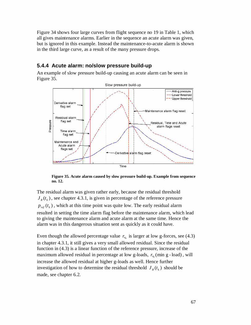
67

Figure 34 shows four large curves from flight sequence no 19 in Table 1, which all gives maintenance alarms. Earlier in the sequence an acute alarm was given, but is ignored in this example. Instead the maintenance-to-acute alarm is shown in the third large curve, as a result of the many pressure drops.

5.4.4 Acute alarm: no/slow pressure build-up An example of slow pressure build-up causing an acute alarm can be seen in Figure 35.

Figure 35. Acute alarm caused by slow pressure build-up. Example from sequence no. 12.

The residual alarm was given rather early, because the residual threshold

)( kR tJ , see chapter 4.3.1, is given in percentage of the reference pressure )( kref tp , which at this time point was quite low. The early residual alarm

resulted in setting the time alarm flag before the maintenance alarm, which lead to giving the maintenance alarm and acute alarm at the same time. Hence the alarm was in this dangerous situation sent as quickly as it could have. Even though the allowed percentage value %r is larger at low g-forces, see (4.3) in chapter 4.3.1, it still gives a very small allowed residual. Since the residual function in (4.3) is a linear function of the reference pressure, increase of the maximum allowed residual in percentage at low g-loads, load)-gmin (%r , will increase the allowed residual at higher g-loads as well. Hence further investigation of how to determine the residual threshold )( kR tJ should be made, see chapter 6.2.

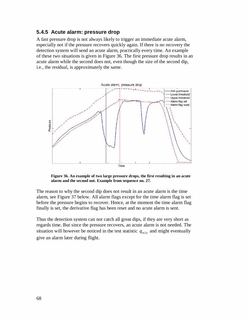
68

5.4.5 Acute alarm: pressure drop A fast pressure drop is not always likely to trigger an immediate acute alarm, especially not if the pressure recovers quickly again. If there is no recovery the detection system will send an acute alarm, practically every time. An example of these two situations is given in Figure 36. The first pressure drop results in an acute alarm while the second does not, even though the size of the second dip, i.e., the residual, is approximately the same.

Figure 36. An example of two large pressure drops, the first resulting in an acute alarm and the second not. Example from sequence no. 27.

The reason to why the second dip does not result in an acute alarm is the time alarm, see Figure 37 below. All alarm flags except for the time alarm flag is set before the pressure begins to recover. Hence, at the moment the time alarm flag finally is set, the derivative flag has been reset and no acute alarm is sent. Thus the detection system can not catch all great dips, if they are very short as regards time. But since the pressure recovers, an acute alarm is not needed. The situation will however be noticed in the test statistic amq 2 and might eventually give an alarm later during flight.

69

Figure 37. A great pressure drop not resulting in an acute alarm due to the quick recovery. Example from sequence no. 27.

5.4.6 Acute alarm: fluctuating depression A pressure signal that is fluctuating, almost noisy-looking, such as the example in Figure 38, often result in several settings and resetting of the derivative alarm flag. Only maintenance and acute alarm flags are presented in the figure, but the right curve also gives six derivative alarms and one extra maintenance alarm besides the four needed alarm flags to set the acute alarm. The left curve, which did not give an acute alarm, gives totally three maintenance alarms, ten derivative alarms, three residual alarms and two time alarms. In this specific case the large pressure drop in the right curve is somewhat larger than the largest pressure drop in the left curve, resulting in the acute alarm. These kinds of fluctuating anti-g pressure sequences can also give rather many maintenance alarms. Every time the pressure signal reenters between the thresholds, which might occur many times due to the quick changes in the signal, the CUSUM test statistic q is reset. The next larger pressure drop will then give a new maintenance alarm. However, many maintenance alarms are a clear indication of a non-reliable PSU, even if an acute alarm is not sent.

70

Figure 38. Fluctuating anti-g depression, resulting in several maintenance alarms and one acute alarm. The two curves look similar, although only the right one causes an acute alarm, due to a somewhat faster and larger pressure drop. Example from sequence no. 19.

5.4.7 Acute alarm: Safety pressure lost (simulation) In order to verify the alarm function described in chapter 4.4.1, a flight sequence was modified to simulate this loss. A small signal sequence at level flight was replaced with a simulated one. The simulated sequence consisted of a small constant value 0 and additive white normal distributed noise, with expected value zero and standard deviation . The detection system was run on the modified sequence, resulting in an acute alarm, see Figure 39. Note that this acute alarm only operates with the parameters safetyt and safetyl , and does not include any sub-alarms.

71

Figure 39. A simulated test to validate the detection system when the safety pressure is lost or too low at level flight.

5.5 Noise sensitivity In order to test how the detection system responds to input signals which are noisier than the provided data, two different simulated noises were added to the original input signals mg and mp . The same filter parameters as for the original system was used, i.e., the system was not adapted to handle this extra noise. The purpose of the test was simply too see what would happened if the input signals where exposed to large noise, i.e., to test the sensitivity of the detection system. The two noise levels used in the test are referred to as medium noise mn and high noise hn . Both are white normal distributed noise with average zero. The medium noise has the standard deviation and the high noise has standard deviation 2 , i.e., ),0(~ Nnm and )2,0(~ Nnh . The -parameter was chosen ad hoc. The result is shown in Table 3 below. The table also includes the noise test result from when using the drift term in the CUSUM-test described in (4.2) in chapter 4.2.1. By using the drift term in the CUSUM-test, the part of the signal that due to noise ends up outside of the allowed pressure area can be subtracted and hence reduce the risk of false alarm. The drift term used in this test was chosen to the half of the medium noise standard deviation, i.e., 2 . However, the choice of drift term value should be investigated further. The test was done with added noise to all of the training data sequences. Four of the sequences are presented in Table 3, two faultless and two with faults, all

72

giving false alarms due to noise. These are chosen as examples of when the detection system does not respond well to noise. However, note that several of the flight sequences with added noise did not give any false alarms at all, or only when using the high noise level, or when not using the drift term.

Flight seq. no.

Noise added / drift term



Comments

None FL FL mn 1 MA

mn , 1 MA

hn 3 MA

2

hn , 3 MA None FL FL

mn 12 MA

mn , 2 MA

hn 16 MA

8

hn , 7 MA

Many false alarms due to several curves with slow inflation

None 1 MA, 2 AA 1 MA, 2 AA mn 1 MA, 2 AA

mn , 1 MA, 2 AA

hn 3 MA, 3 AA Gives 2 extra MA

12

hn , 3 AA None 1 MA, 2 AA 2 MA, 1 AA

mn 2 MA, 1 AA

mn , 1 MA, 1 AA

hn 1 MA, 1 AA

14

hn , 1 MA 1 AA

Missed detection of one MA

Table 3. The results from testing the detection system using added noise to the training data. Here four sequences which gives false alarms are presented, two faultless and two with faults.

In five of the ten faultless sequences the added noise mn and hn , one or both, did not give any false alarms, no matter the noise level. The other five faultless sequences did however result in one or several false alarms due to noise. Two of them, sequence no 2 and 8, are shown in Table 3. In these situations only false maintenance alarms were given, not acute ones. Sequence no 8 resulted in many maintenance alarms when the drift term was not used, mainly due to slow inflation at increasing g-load.

73

The added noise to the faulty sequences often, but not always, resulted in extra alarms. In sequence no 12 in Table 3 the added high noise resulted in interpreting a maintenance alarm as an acute alarm. However, in sequence no 14 the line between the different alarm situations is vague, and there the added noise resulted in a missed detection of a maintenance alarm. Otherwise there was no missed detection. The use of drift term in the CUSUM-test often improved the result, especially for the high noise, or gave the same results. Hence the drift term should be used if the signals are exposed to larger noise than the original signals of this thesis. However the use of drift term on the original signals will only delay the alarm time point, which is not needed. The false maintenance alarm situations mostly occurs when the original pressure signal is close to, or temporary outside, one of the thresholds. It specially occurs when the g-force increases and the inflation is slow. This happens during sequence no 8 in Table 3, and two of the false maintenance alarms can be seen below in Figure 40. The upper figure shows the faultless pressure signal without added noise, giving no alarms. Below the pressure with added medium noise mn is shown, giving false maintenance alarms. No drift term was used. The noise inflicts the residual mins and larger residual values add up the test statistic q faster.

Figure 40. Above: A piece of the faultless sequence no 8 in Table 3. The pressure signal is occasionally quite close to the lower threshold due to slow inflation, but no alarms are given. Below: The same signal with added noise, resulting in false maintenance alarms.

The noise also affects the sub-alarms. The residual at time kt can be, due to the added noise, both larger and smaller than otherwise, which affects the residual alarm flag and the CUSUM test statistic. In sequence no. 14 in Table 3 this

74

situation results in a missed detection of a maintenance alarm. The derivative alarm flag is also set and reset several more times due to the quick changes in the noisy signal. Hence a false acute alarm might be sent in a situation such as described in chapter 4.3.4, Figure 29, where the derivative difference for the none-noisy signal is small and no acute alarm is needed. Then a maintenance alarm can be misinterpreted as an acute alarm.

5.6 Maintenance false alarms risk due to the adapted thresholds

The adapted thresholds shifts from being the filtered static threshold to being the original static threshold, see chapter 3.4.3. These shifts often result in a sudden, sometimes relatively large change of threshold value between two samples. An example of this can be seen in the lower adapted threshold in Figure 41. The shifts occur due to a change of derivative sign of the reference pressure, which decides whether the filtered static threshold or the original static threshold should be used. However, in Figure 41 the adapted threshold soon shifted back again, making the shift appear to be rather unnecessary. The momentarily increase of threshold value suddenly left the anti-g pressure outside the allowed pressure area. This resulted in a positive residual mins , adding up the CUSUM test statistic minq , which eventually leads to a maintenance alarm, , see (4.2) in chapter 4.2.1. If the sudden shift in the lower adapted threshold had not occurred, the alarm would not have come at all, or would have come later, during this temporary threshold trespassing of the anti-g pressure. A way to avoid unnecessary temporary shifts in the adapted threshold is to test whether a potential shift is needed or not. This can be done by “pausing” the filter process for a few samples to see what happens to the derivative sign. How the test algorithm can work is described in Appendix A, where the solution was developed but not used in this thesis. However, pausing of the filter process also means pausing of the detection system, i.e., potential alarms given by the detection system during the test period will be delayed. This is further discussed in Appendix A. During the tests and evaluations in chapter 5, most of the given maintenance alarms have been justified according to the author and Saab employees, others have been somewhat doubtful. In these cases it is a matter of subjective judgment. How often the maintenance alarms are given due to the situation described in Figure 41, either falsely or too early, needs to be investigated further, see chapter 6.2.

75

Figure 41. A maintenance alarm most likely caused by the shift in the adapted threshold. The lower adapted threshold went from being the filtered static threshold to being the original one, causing a momentarily increase of threshold value. The sudden increase in residual affects the CUSUM test, where the CUSUM threshold will be exceeded earlier than expected. Example from sequence no. 23.

76

6 Summary and future work 6.1 Summary In this thesis a system for monitoring and fault detection of an anti-g protection system has been developed, in order to increase flight safety. The values of the input signals, anti-g pressure and g-load, were taken from real flight sessions and the sensor values were assumed to be correct. The thresholds, in which between the anti-g pressure should lie in a faultless system, are calculated from the g-load value. The thresholds are based upon given static guidelines for the anti-g pressure tolerance area. However, the anti-g protection system has certain dynamics and has been estimated as a first order system. Hence the static thresholds have been modified in order to adapt to this dynamics, and defines the pressure thresholds used in the detection system. The detection system gives two kinds of alarm; maintenance and acute. The system distinguishes the alarms through different tests and conditions. The maintenance alarm is given at minor, but still serious pressure deviations. The alarms are accumulated and can result in an acute alarm if they occur too often. The acute alarm is also given at grave pressure deviations as well as at loss of safety pressure. The alarm conditions are parameter controlled and can easily be tuned. The validation has been performed using both faultless and faulty flight sequences, visually determined by Saab employees. The validation of faultless data showed that a few false maintenance alarms occurred. However the line between faultless and maintenance alarms was in those cases considered to be vague. Most of the faultless flight sequences gave no alarms at all. The detection system has also been tested using input signals with simulated extra noise, showing some sensitivity, especially towards large noise. False alarms, maintenance alarm in particular, occurred, but rarely any missed detections. In all faulty flight sequences at validation the detection system has given the right kind of alarm according to Saab employees, and hence no false alarms. Nor were there any missed detections. All together the detection system is considered to work well.

6.2 Future work/Alternative solutions Here a few suggestions of further work in order to improve the detection system are presented, as well as some alternative solutions:

77

System order estimation In this thesis the dynamics of the PSU and anti-g trousers were approximated as a first order system. Further investigation might be of interest to get a more precise approximation of the dynamics. Model based diagnosis With a physical model of the PSU and anti-g trousers the detection system could also include diagnosis statements and fault isolation of, for example, system components. This could make the maintenance work easier. Sensor diagnosis In this thesis the pressure sensor is assumed to give a correct value. However, a sensor can not always be expected to function properly and therefore the system should include sensor diagnosis as well. Derivative estimation The basic derivative estimation used in this thesis might not be good enough if the signal includes larger noise. In that case other derivative estimation methods should be investigated. One method is the smoothing spline approximation, described in [7]. Monitoring pilot’s condition Instead of just fault detection of the anti-g protection system, the pilot’s condition during high g-load exposure can be diagnosed and corrected, as described in [8]. Separate maintenance alarm condition from acute alarm The tuning process of the CUSUM threshold for the maintenance alarm might be somewhat difficult when it is also used as a condition to the acute alarm. Instead two CUSUM threshold can be used; one only for maintenance alarm and one used for acute alarm. The CUSUM-test condition for acute alarm might also be removed completely if necessary. Shifts in adapted thresholds The quick shifts from filtered to static threshold that occurs during the threshold adaption, which causes sudden “jumps” in the threshold, should be smoothened in some way. One solution is presented in Appendix A, but further investigation might be of interest. Detecting fluctuating pressure between thresholds A fluctuating pressure signal at a constant g-load might indicate a PSU malfunction. The detection system in this thesis will not detect this behavior if the pressure still remains between the thresholds. Therefore a method of detecting the fluctuation could be added to the detection system, in order to get an earlier indication of an unreliable PSU.

78

Defining allowed pressure deviation Further investigation in order to define how large a pressure deviation can be before it is considered an immediate danger should be made, e.g., by consulting a medical officer. Vary CUSUM threshold for maintenance-to-acute alarm The CUSUM threshold used in the maintenance-to-acute alarm can be difficult to tune when the length of flight varies. The test statistic could for example be reset if no maintenance alarm has been given during a certain length of time, or could be normalized by time. Noisier input signals If the input signals to the system are measured differently from the data provided for this thesis, the need of further noise reduction and signal processing should be investigated.

80

Nomenclature Abbreviations

Description

AIU Aircraft Interface Unit BEOS Back-up & Emergency Oxygen Supply CUSUM Cumulative Sum ECS Environmental Control System EWMA Exponentially Weighted Moving Average NRMSE Normalized Root Mean Square Error OBOG Onboard Oxygen Generator PRV Pressure Regulating Valve PSU Pilot Service Unit RMSE Root Mean Square Error WDV Water Drain Valve Parameters

Description Unit

a , Filter parameters - D Derivative difference fa pl min, kPa/s

Af Alarm flag, acute alarm -

Df Alarm flag, derivative alarm -

amf 2 Alarm flag, maintenance-to-acute alarm -

max,Mf Alarm flag, maintenance alarm, overpressure -

min,Mf Alarm flag, maintenance alarm, depression -

Rf Alarm flag, residual alarm -

Tf Alarm flag, time alarm -

fg Measured g-force, filtered G

mg Measured g-force, unfiltered G

DJ Derivative alarm threshold -

amJ 2 CUSUM threshold, maintenance-to-acute alarm -

maxJ CUSUM threshold, maintenance alarm, overpressure -

minJ CUSUM threshold, maintenance alarm, depression -

RJ Residual alarm threshold -

TJ Time alarm threshold -

max,al Upper adapted threshold kPa

min,al Lower adapted threshold kPa

min,al Derivative of lower adapted threshold kPa/s

min,sl Lower static threshold kPa

81

max,sl Upper static threshold kPa

safetyl Pressure limit, loss of safety pressure kPa

min,testl Lower test-threshold kPa

max,testl Lower test-threshold kPa

fp Measured anti-g pressure, filtered kPa

fp Derivative of measured filtered anti-g pressure kPa

mp Measured anti-g pressure, unfiltered kPa

refp Anti-g reference pressure kPa

refp Derivative of anti-g reference pressure kPa/s

amq 2 CUSUM test statistic, maintenance-to-acute alarm -

maxq CUSUM test statistic, overpressure -

minq CUSUM test statistic, depression -

maxs Residual overpressure max,af lp kPa

mins Residual depression fa pl min, kPa

alarmt Time parameter in time alarm -

kt Time at sample k s

safetyt Time limit, loss of safety pressure s

sT Sample period s Time constant s

82

References [1] Basseville, M. and Nikiforov, I.V., Detection of Abrupt Changes - Theory and Application, Prentice-Hall, Inc., Englewood Cliffs, N.J., (1993). ISBN 0-13-126780-9. [2] Gustafsson, F., Adaptive filtering and Change Detection, John Wiley & Sons, Ltd, (2000). ISBN 0-471-49287-6. [3] Gustafsson, F., Ljung, L. and Millnert, M., Signalbehandling, Studentlitteratur (2001). ISBN 91-44-01709. [4] Page, E.S., Continuous inspection schemes, Biometrika, 41:100-115, 1954. [5] Söderkvist S., Tidsdiskreta signaler och system, 3:e upplagan, (2005). [6] Ljung, L. and Glad, T., Modellbygge och Simulering, Studentlitteratur (2004), ISBN 91-44-02443-6 [7] Kingstedt, J. and Johansson, M., Methods for Residual Generation Using Mixed Causality in Model Based Diagnosis, Master’s thesis, Dept. of Electrical Engineering, Linköping 2008. Reg.no: LITH-ISY-EX--08/4882--SE [8] Vasiletz, V.V. and Yakimenko, O.A., The concept of on-board diagnostics, prognosis and correction of pilot condition under the action of high level G-load complex, Aerospace and Electronics Conference, NAECON, 1995. [9] Saab AB homepage, http://www.saabgroup.com, 2010-02-19 Saab documents [10] On Board Oxygen Generation System (OBOGS) and Anti-g system, JB035-05-SP:30221 F/ISC Issue 1c [11] Flp 39C och 39D. Dimensionerade krav på anti-g-funktionen, JSA-32-BJ:410FH [12] Reglering av g-dräktstryck. SYSIM-modell, TUSL-39-94:267 [13] Flp JAS39. Funktionsövervakning av g-dräktstryck. Specificering och verifering, JSK8-32-RA:1001 [14] Protokoll, JSK8-32-RA:1144

84

Appendix A: Adaptive filtering of the thresholds using Test mode The filter process algorithm of the adapted thresholds is described in 3.4.3. To this algorithm an extra filter mode can be added, called the Test mode. The Test mode will handle the change of derivative signs differently; instead of just immediately shifting between filtered static threshold and original static threshold this mode will test whether a shift really is necessary. A.1 Special solution: change of derivative sign If the g-load changes from an increase to decrease and vice versa, there will be a shift of the static threshold that should be filtered. However, a change of derivative sign between two samples could be a result of noise, or just be a very short temporary change. A shift of filtered threshold is not necessarily needed during these few samples, instead there is a risk of false alarm, see Figure 42. The risk of these shifts is also mentioned in chapter 5.6.

Figure 42. A temporary change of derivative sign causes an unnecessary shift of filtered threshold, in this case a shift from the upper static threshold to the lower one. The upper adapted threshold is set to the static threshold, risking a false alarm in the process.

A solution to this situation is to “pause” the filtering decisions for a short time and evaluate if the change in derivative sign is temporary or not, based on which derivative sign is most frequent during this time. In case a shift really is needed, the transition can be smoother by letting the present filtered threshold continue to be filtered a few samples even after the shift occurred. Naturally this “pause”,

85

or test period, will cause a delay in detection of faults, further described A.4 below, and should be kept as small as possible. A.2 The filter algorithm including Test Mode The algorithm will besides the filter modes described in chapter 3.4.4 also include change of sign-mode and test mode.

Figure 43. Schematic view of the Adapted Thresholds Algorithm including special change of sign solution.

86

Change of Sign mode If the derivative signs do not fit with any of the other modes, they must be of different signs, i.e., one is positive and the other is negative. This change of sign could just be a result of a disturbance or an otherwise insignificant change in the

refp -signal and therefore a shift of filter mode, always between Positive and Negative mode, might not be needed. In this situation the algorithm will prepare for Test mode by setting a test flag, which will “pause” the filtering decisions to evaluate if a shift of filter modes is necessary, see description below. Test mode As long as the test flag is set, the algorithm will keep entering Test mode for an in advanced chosen number of samples, i.e., the filter decisions will be “paused” for the time corresponding to these samples. The test amounts to evaluate whether the derivative signs during these samples are mostly positive or negative, and the most frequent sign represent the filter mode that should be used, Positive or Negative. The test ignores the derivative signs that are considered to be zero since, during the relatively short test period, a shift to Zero mode is irrelevant. When the test period has come to its end, the test flag will be unset and a filter mode for the test period samples will be chosen. However, in order to make the transition from the earlier filter mode into the test period smoother, the adapted thresholds will both be the filtered static thresholds at the beginning of the test period sequence. The latter parts will be set as in Positive or Negative mode, depending on which filter mode was chosen. Since the Test mode result can be either Positive mode or Negative mode, two pairs of adapted thresholds need to be available at the end of the test; one pair with a filtered lower static threshold and an un-filtered upper one for Positive mode, and one pair with a filtered upper static threshold and an un-filtered lower one for Negative mode. The filtered upper and lower thresholds created during the test period are called the test thresholds, min,testl and max,testl . The Test mode will cause a certain delay before any fault detection can be made, hence the test period should not be longer than an accepted delay. The Test mode filter process can be seen in Figure 44.

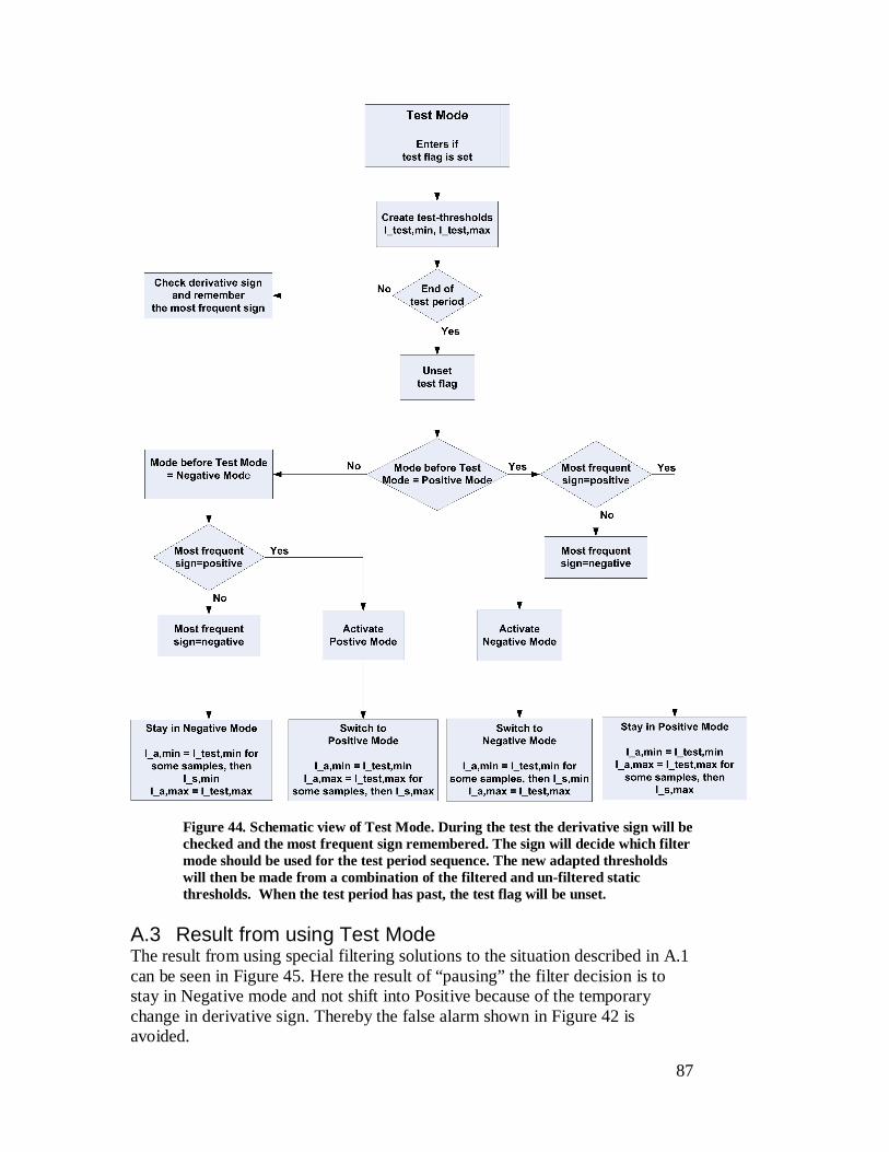
87

Figure 44. Schematic view of Test Mode. During the test the derivative sign will be checked and the most frequent sign remembered. The sign will decide which filter mode should be used for the test period sequence. The new adapted thresholds will then be made from a combination of the filtered and un-filtered static thresholds. When the test period has past, the test flag will be unset.

A.3 Result from using Test Mode The result from using special filtering solutions to the situation described in A.1 can be seen in Figure 45. Here the result of “pausing” the filter decision is to stay in Negative mode and not shift into Positive because of the temporary change in derivative sign. Thereby the false alarm shown in Figure 42 is avoided.

88

Figure 45. The temporary change of derivative sign of the reference pressure “pauses” the filter decisions for a short period and evaluates if a shift from Negative mode to Positive mode is necessary. In this case the decision is to stay in Negative mode and by doing so avoid false alarm.

A.4 Consequences of using Test mode By using Test mode the filter process of the adapted thresholds will be paused several times during a flight sequence. Hence the threshold values during the test period will not be set until the period is over. This also affects the detection system, which uses the adapted threshold values to make its alarm decisions. If an alarm should be given based upon the filter result from Test mode, it will not be sent until the test period is over. In worst case the alarm can be delayed for as long as the test period. The test period can of course be shortened, but if it is too short the purpose of using Test mode is lost. A compromise between a long test period and a short alarm delay is needed. Further analysis of an accepted alarm delay should be done before using Test mode in the filter algorithm of the adapted thresholds.

lith-isy-ex--10/4270--se linköping 2010 · loads. in order to prevent the draining of blood from...

Documents