SWARTHMORE COLLEGE

DEPARTMENT OF ENGINEERING

SENIOR DESIGN PROJECT

Live RSSI Mapping System

AuthorsTimothy NGUYEN

Neeraj SHAH

SupervisorMatt ZUCKER

IN PARTIAL FULFILLMENT OF THE REQUIREMENTS

FOR THE

DEGREE OF BACHELORS OF SCIENCE

May 10, 2019

i

Abstract

For our final engineering project, we wanted to explore a quality assuranceproblem related to networking. We successfully built a heat-map that intuitivelydisplays the strength of wireless signals. The project has two major components:a Raspberry Pi and an AWS-based server. The Pi acts as a measurement devicefor signal strength and the server receives and processes the Pi’s data to generatea map. The project is optimized for real-time updates and has features that canisolate the strength of individual routers.

ii

Acknowledgements

We would like to thank Professor Matt Zucker for mentoring our project. His input andfeedback helped us constantly move forward. We also would like to thank the engineeringdepartment for helping us obtain materials and for facilitating the entire project.

iii

Contents

1 Introduction 1

2 Raspberry Pi 12.1 GPS . . . . . . . . . . . . . . . . . . . . . . . . . . . . . . . . . . . . . . . . . . . . . 12.2 Wireless Monitoring . . . . . . . . . . . . . . . . . . . . . . . . . . . . . . . . . . . 22.3 Handling the Data . . . . . . . . . . . . . . . . . . . . . . . . . . . . . . . . . . . . 32.4 JSON Format . . . . . . . . . . . . . . . . . . . . . . . . . . . . . . . . . . . . . . . . 32.5 Additional Hardware . . . . . . . . . . . . . . . . . . . . . . . . . . . . . . . . . . . 3

3 Lightsail Server 43.1 Cloud . . . . . . . . . . . . . . . . . . . . . . . . . . . . . . . . . . . . . . . . . . . . 43.2 Map Generation Theory . . . . . . . . . . . . . . . . . . . . . . . . . . . . . . . . . 43.3 Data Processing . . . . . . . . . . . . . . . . . . . . . . . . . . . . . . . . . . . . . . 53.4 Image Generation . . . . . . . . . . . . . . . . . . . . . . . . . . . . . . . . . . . . . 53.5 Python Script Optimization . . . . . . . . . . . . . . . . . . . . . . . . . . . . . . . 63.6 MAC Address-Based Heatmap . . . . . . . . . . . . . . . . . . . . . . . . . . . . . 73.7 Web Development . . . . . . . . . . . . . . . . . . . . . . . . . . . . . . . . . . . . . 83.8 Google Maps API . . . . . . . . . . . . . . . . . . . . . . . . . . . . . . . . . . . . . 83.9 Hosting Files with Node JS . . . . . . . . . . . . . . . . . . . . . . . . . . . . . . . 9

4 Results 9

5 Future Work 11

6 Appendix 116.1 Python Code on Raspberry Pi . . . . . . . . . . . . . . . . . . . . . . . . . . . . . . 116.2 Python Code on Server . . . . . . . . . . . . . . . . . . . . . . . . . . . . . . . . . . 13

iv

List of Abbreviations

RSSI Received Signal Strength Indication

MAC Media Access Control

BSS Basic Service Set

SSID Service Set Identifier

DBM Received Signal Strength Indication

AWS Amazon Web Services

JSON Javascript Object Notation

API Application Programming Interface

1

1 Introduction

As our connection to the internet becomes increasingly important and as new forms of dispens-ing internet services emerge, it is important to identify weak-spots in any internet network. Wepropose developing Raspberry Pi devices which will continuously monitor the strength of aWiFi signal (Eduroam in our case) and output the values to a web application to continuouslyupdate a heatmap. As the devices move around campus, the heatmap will then show areas ofweak and strong coverage.

We can imagine a system where multiple people, at different points around Swarthmore,roam the campus and provide valuable data to students, professors, and network engineers onthe current state of Eduroam. This will allow everyone to identify the exact location of deadspots or areas of weak coverage. We hope that the final system can be used for identifyingweak spots on larger scale networks like LTE or satellite based internet services.

We will rely on common signal strength measurements like Received Signal Strength Indi-cator (RSSI) to quantitatively represent different areas on campus. These can be outputted withthe linux module iw. We will also obtain locations for these readings with the GPS module at-tached to our Pi. All readings will have associated degrees of confidence that can be improvedover time.

This is an interesting problem to solve because of how it applies many engineering disci-plines to tackle a common issue. We would be using knowledge of networks, hardware-design,probabilistic models, and software engineering principles to approach this task.

The project can be broken down into two major components. The first revolves around theRaspberry Pi and its associated hardware extensions. The Pi handles all of the data collection.The second component relates to our server, which processes all of the data and ultimatelyserves a web page to the user, displaying all of the information about the current state of thewireless network in question.

2 Raspberry Pi

Our choice for processing inputs was a Raspberry Pi 3B+, running the latest version of Rasp-bian OS. This is a Unix-like OS, giving us the full functionality of a UNIX command line.

2.1 GPS

In order to keep track of our location, we purchased an Adafruit Ultimate GPS Breakout mod-ule which outputs latitude, longitude, and altitude with a 10Hz update frequency. This GPSmodule was connected to the Pi via a USB Serial connection. The GPS module can be seen infigure 1. Four pins on the GPS were wired to the Pi: TX, RX, GND, and VIN.

2

Figure 1: Ultimate GPS Breakout Module

Originally, this GPS module was not en-tirely accurate, giving an error of over 30 me-ters. In order to remedy this, an additionalantenna was purchased for the GPS unit, in-creasing the rate at which it fixed to satel-lites and improving indoor and outdoor pre-cision.

2.2 Wireless Monitoring

Across most UNIX distros, the iw commandcomes pre-installed. This is a new command line utility for wireless devices. This commandoften gets confused with iwconfig, a now deprecated tool. The new iw utility handles newergenerations networking protocols. The commmand that we run on our Pi is

iw dev wlan0 scan

The command invokes the iw utility with the first word. The second word, dev, stands fordevice. The third word, wlan0, specifies which device we want to look at. In most modernmachines, wlan0 refers to the integrated networking card. The last word, scan, looks at all theavailable networks and outputs their details.

The output of this command is all the wireless networks the Pi can pick up and all of itsassociated metadata. The only information we are interested in are the SSIDs, MAC addresses,and signal strengths. So we filter the results by those fields with the following extension to ouroriginal command:

iw dev wlan0 scan | egrep “∧BSS|Signal|SSID”

Figure 2: Output of iw Command

sudo iw dev wlan0 scan I egrep ""BSSlsignallSSID" c8:b5:ad:34:38:60(on wlan0)

: -68. 00 dBm : eduroam

c8:b5:ad:34:38:62(on wlan0) : -69 . 00 dBm

: SwatGuest cH:b5:ad:34:d1:10(on wlan0)

: - 57 . 00 dBm : eduroam

c8:b5:ad:34:d1:12(on wlan0) : -57 . 00 dBm

: SwatGuest c8:b5:ad:34:e7:80(on wlan0)

-72 . 00 dBm : eduroam

c8:b5:ad:34:e7:82(on wlan0) : - 71.00 dBm

: SwatGuest c8:b5:ad:34:3a:62(on wlan0)

: -81 . 00 dBm

3

2.3 Handling the Data

The entirety of the data collection is done in one Python script, which handles the GPS andWiFi data. The GPS data is obtained with a library known as AGPS3. Originally, we used thelibrary associated with Adafruit; however, we quickly ran into an issue where a backlog ofolder GPS readings were being saved. This was solved in the newer library with threading.Threading is a tactic employed by programmers to speed up computation for a single process.This new library had threads that handled clearing the old buffer that accumulated overtime.

Once the GPS data was streaming in real time, we incorporated the WiFi data previouslymentioned. In order to run the shell command in Python, we utilized a builtin library calledsubprocess. This enables us to run these shell commands as processes from Python and col-lect their output. Thus, for every iteration that we grab a GPS reading, we also run the shellcommand and obtain the associated WiFi data.

2.4 JSON Format

After obtaining the GPS and WiFi data every iteration, we must parse through the data, ensureit’s properly formatted and free of errors, and package it into a readable format. The format wechose was a JSON file. JSON format is the industry standard for transferring data between webapplications and servers, storing the data as readable tree of nested dictionaries and lists. Aswe traverse around campus and gather data, our JSON file will continue to grow, eventuallyreaching over 100,000 lines. This occurs because in addition to saving data for Eduroam, wealso hold the data for SwatGuest and SwatDevice. This was a design choice, should we chooseto extend our project to other SSIDs as well.

In order to handle random bugs and program interruptions, we have a fail-safe protocol:every 100 iterations, we will save the current copy of our JSON data. Once we have finishedall of the data collection, the Python script will push the final JSON file to our AWS server.

2.5 Additional Hardware

While traversing campus, we required a constant source of power to keep the Raspberry Pirunning. We purchased an additional battery pack from the official Adafruit site. The choiceof battery pack is important because the Raspberry Pi may run into undervoltage issues if notprovided a consistent 5V source. Additionally, the cable to power our Pi must be as short aspossible, since longer cables tend to have a higher resistance.

Furthermore, an additional touchscreen monitor was purchased to monitor the output ofthe program on the go.

4

3 Lightsail Server

3.1 Cloud

In order to serve our desired product to the end-user, we must have a place where we canperform the computationally intensive task of producing the heatmap and hosting our web-site files. Cloud based storage is becoming an increasingly popular choice for consumers andcompanies to store data. As opposed to traditional storage methods which involve owninglarge racks of hard-disks on site, cloud storage takes away local storage and hosts your data ina remote location with an easy, intuitive way to interact with it.

The cloud provider we chose for our project is Amazon and their AWS services. AWS offersnumerous amounts of services for different needs. However, we opted for a service calledLightsail, which can simply be thought of as a remote computer. Lightsail gives us access toan always-on computer in one of Amazon’s facilities in Virginia, providing us with 16 GBs ofRAM, 4 vCPUs, and 320 GBs of flash storage. The computer is running Ubuntu 18.04 as itsoperating system. Our cloud instance has the static IP address:

18.206.136.194

3.2 Map Generation Theory

Before we get into the Python scripts running on the server, let’s talk about the theory behindour heatmap generation. Recall that after our Pi compiles all of the data into a JSON format,it’s pushed onto our server for further processing. The JSON file contains hundreds of points,each characterized by a latitude, longitude, and a list of all the wireless networks seen by thePi at that point.

Since we are gathering data across campus, it is impossible to get the signal strength at ev-ery possible latitude and longitude. As such, we are confronted with the problem of estimatingthe strength at points we don’t have data for. This motivates a need for an interpolation-basedapproach.

For interpolation, we use a locally weighted regression. We center a 3-dimensional Gaus-sian distribution on each measured point. The distribution values represent how much weighteach measurement contributes to the prediction of another point. For every point we are tryingto predict, we will use these weights to take a weighted average of measured values. As ex-pected, points near a measured point will be more likely to reflect that point’s measured valuethan points further away. We can think of the Gaussian distributions as confidence intervalsover each point.

To formalize, the distribution that belongs to a particular measurement at point µ will bedefined by f:

f ∼ N(µ,σ2) (1)

5

where σ2 is some constant we define and represents the size of the confidence interval for eachmeasurement.

At some other point j, we can then interpolate a value by utilizing all our measured points.

valuej =∑n

i=1 weights ∗ fi

∑ni=1 weights

(2)

where i ∈ S, the set of all measured points.We can populate an entire map of the region of interest with values using this interpolation

map. We decide which values to populate by using a grid-based approach. We color-code ourmap to visually reflect the signal strengths we see.

3.3 Data Processing

Our JSON file is composed of longitude/latitude values. These are not intuitive or relatableunits. Ultimately, our map generation algorithm relies on parameters like σ, which representsdistance. To better understand and vary such parameters, it is helpful to have all our coordi-nates in meters. Additionally, since the differences between GPS values depend on where youare on earth, parameters like σ would need to vary based on your location too. Because of this,we chose to convert all latitude and longitude values to the Universal Transverse Mercator Co-ordinate System, which is measured in meters and is spatially-consistent regardless of whereyou are on earth. Python has a utm library which facilitates this unit conversion.

3.4 Image Generation

The image generation is governed by one main Python script. This script reads in the JSONfile pushed from the Pi, isolates the SSIDs we want to focus on (Eduroam in our case), convertsGPS coordinates to UTM coordinates, and generates a heatmap based on the theory presentedearlier. To build our main map, we select Eduroam signals that are the strongest at each point.We then populate the map by following the map generation algorithm at each square in a pre-defined grid. The squares of the grid represent the individual pixels that our algorithm willeventually output.

6

Figure 3: Example grid to Populate

Once we have populated our grid with values, we have to map the values to intuitivecolors. To do this, we normalize our values so that they are all between 0 and 1. Then, weobtain pixel values for our red, green, and blue values by applying a sinusoid function withchanging parameters for each color as shown in equation 3. We made the sinusoid for thered-values peak at 1, the sinusoid for the blue-values peak at 0, and the the sinusoid for thegreen-values peak at 1/2.

a + b ∗ cos(2 ∗ π ∗ (c ∗ val + d))) (3)

3.5 Python Script Optimization

The calculations for the locally weighted regression are time and memory intensive. Since wedetermine every single measurement’s contribution to each point in our grid, our run-time isO(lwn). l is the number of rows in our grid, w is the number of columns in our grid, and n isthe number of entries from our JSON file.

Normally, we would execute this in python via three nested "for" loops. To speed up ourcode, we relied on the numpy library in python which allowed us to use C-based code andmatrix operations. We used the meshgrid command to build a matrix for our grid and builtanother matrix for our measurements. By multiplying the matrices together with broadcasting,we were able to create a three-dimensional "weights" matrix which had dimensions l ∗ w ∗ n.We could then produce the desired results by using a sum function along the second axis.

This vectorization sped up our code significantly, but we soon realized that we wouldrun into memory errors if the size of the "weights" matrix grew too large. Because of this,we performed our calculations on small portions of the grid and created smaller "weights"matrices. We would delete each "weights" matrix once it produced the desired results. Thisprocess is called "chunking".

I>.

I •

~ ,

-'

J_ . -9

7

Figure 4: Image Generated by Script

3.6 MAC Address-Based Heatmap

One topic we wanted to explore is localization based on signal strength. To begin to solvethis problem we isolated the strength of specific routers. We saw that signal strength tends totaper off as we move away from a router. This understanding could help us build probabilisticmodels to discover where routers are and, following that, where we are. In future work, wewould like to analyze these visualizations more closely.

8

Figure 5: Single MAC Address Image Generated by Script

3.7 Web Development

Upon the completion of the image generation, we obtain a PNG image to be overlaid overa map of Swarthmore. In order to present this data to the public, we opted to create a webapplication on our AWS server. The website consists of three basic files: HTML, CSS, JS. TheHTML file is what is rendered on the user’s browser. The CSS file helps with aligning the objectson the site. And finally, the JS file handles the communication with Google to obtain a map ofSwarthmore and ultimately overlays the PNG image over it.

3.8 Google Maps API

To display Google’s map on our site, we must communicate with the API that Google Mapsprovides. The term API defines a set of functions that are provided to us in order to accessGoogle’s features. So in our case, we reference Google Map’s library in our HTML code byproviding a private key, allowing us to render their map. The reference to Google Maps in ourHTML code can be seen below:

<script src="https://maps.googleapis.com/maps/api/js?key=<KEY-HERE>

&libraries=visualization"></script>

Upon rendering the map, we must overlay the image generated with the Python code. Thisis done through a series of custom overlay functions provided by Google’s OverlayView class.These functions allow us to manually customize <div> elements in our HTML code, which wedefine to render the map and custom overlay. Additionally, our map shows some additionalinformation for some buildings, which we outlined with red polygons. These polygons are

9

defined with Google’s Polygon class. Upon a mouse hover event, an InfoWindow appears,informing the user how many routers are in that building.

3.9 Hosting Files with Node JS

In order to serve all the website to the end user, we must have a continuously running webserver on our Lightsail instance. Our web server of choice was NodeJS, a popular standardacross many industries. At the core of it, NodeJS, when given a directory, automatically pushesthe webpage to the user, handling all of the HTML headers and data payload processing for us.By default, it looks for a file named index.html to display on the browser. We additionallyspecify a port to forward the site to in our configuration file. In our case, Lightsail has ports22, 80, 8000 open, so we choose 80.

4 Results

We were able to successfully produce a heat-map and overlay it on Google Maps. We also wereable to implement several additional features such as filtering by a single MAC address, click-ing on a point in the map to view its associated signal strength, and hovering over buildingsto display the number of routers. . Our site is currently running at:

18.206.136.194

Figure 6: Example view on the Website

Swarthmore 1,;onege Science Center

9

mg Music Build ing t

Crum Woods

-!all c;>

Lang Perfo rmmg Arts Center

9 Wharton Hall

>(

- (

19 Hall

AT~ .

Pearson Hall c;> Black Cultural Ce1

Winter Garden

Rose Garden

Scott Arboretum of Swarthmore

College

' c;> McCabe Library

Magill Walk Swarthmore Adniiss ions

Visitor Parking

Swarthm ore Colleg e

V,:ii1tor'1 ~ter Rd c;> @

Sharples Dr .. ial,

9 oan~ all ! I

; \~<.: l.. ·, /! "'•1111r1 ' I

Shai-9\e5 \..~ I

10

Figure 7: Access Point Outlines for Buildings

Figure 8: Signal Output via Click (Black Dot)

Water Tower Parking

Cornell Scien :ngineering Lib

•

Lang Music Building

X

Sci Center Sci Center contains 72 access points

Lang Perform ing Arts Center

-53 .920897454612785

1t Parking j l \

\ 'I.

\~ $~\ Pearson H

/ '

Ro

Close

11

5 Future Work

In the future, we would like to extend this project to use multiple Pi’s that potentially com-municate with each other. We would also like to add some optimizations that make it usablefor large scale networks like LTE. Additionally, we would like to continue exploring the local-ization problem and see if we can obtain a solution that increases the spatial accuracy of ourmap.

6 Appendix

Note: JavaScript and HTML code not included in Appendices.

6.1 Python Code on Raspberry Pi

1 from gps3.agps3threaded import AGPS3mechanism2 import os3 import time4 import sys5 import json6 import subprocess7

8

9 def getWifi():10

11 command = ’sudo iw dev wlan0 scan | egrep "^BSS|signal|SSID"’12 while(True):13 try:14 result = subprocess.check_output(command, shell=True)15 break16 except:17 continue18

19 result = str(result)[2::].replace(’(on wlan0)’,"")20 result = result.replace(’\\n’,’ ’)21 result = result.replace(’\\t’,’’).replace(’dBm’, ’’).replace(’SSID:’,’’).replace(’BSS’,’’).

replace(’signal:’,’’)22

23 result = result.split()[:-1]24 tempDict = {}25 wifiList = []26 prevKey = ’’27 i = 028

29 # MAC Address is key. Value is [dBm,SSId]30 while i < len(result)-2:

12

31

32 if (result[i].count(’:’) == 5):33 if tempDict:34 wifiList.append(tempDict)35 tempDict = {}36 tempDict[’MAC’] = result[i]37 tempDict[’DBM’] = result[i+1]38 tempDict[’SSID’] = result[i+2]39 i += 340

41 # Handle cases where SSID has spaces42 else:43 tempDict[’SSID’] += ’ ’ + result[i]44 i += 145

46 return wifiList47

48

49 if __name__ == ’__main__’:50

51 agps_thread = AGPS3mechanism() # Instantiate AGPS3 Mechanisms52 agps_thread.stream_data() # From localhost (), or other hosts, by example, (host=’gps.ddns

.net’)53 agps_thread.run_thread() # Throttle time to sleep after an empty lookup, default ’()’ 0.2

two tenths of a second54 outerDict = {"JsonData":[]}55 i = 056 while 1:57 temp = agps_thread.data_stream58

59 data = {}60 data["wifi"] = getWifi()61 data[’Latitude’] = temp.lat62 data[’Longitude’] = temp.lon63 data[’Altitude’] = temp.alt64 print("Iteration : %d %s %s" %(i, data[’Latitude’], data[’Longitude’]))65

66 i += 167 outerDict["JsonData"].append(data)68 if (i%100 == 0):69 print("Dumping %s" %(str(i)))70 name = str(i) + ’_wifi_gps_data.json’71 with open(name,’w’) as outfile:72 json.dump(outerDict, outfile, indent=4)73 print("Written!")74

75 # i = howevery many iterations we want to walk for

13

76 if (i == 500):77 print("Writing to AWS..")78 # command = ’scp -i LightsailDefaultKey-us-east-1.pem wifi_gps_data.json ubuntu@54

.89.88.216:~/e90/public’79 # os.system(command)80 with open(’test_sleep.json’,’w’) as outfile:81 json.dump(outerDict, outfile, indent=4)82 print("Written!")83 exit(1)84 i = 085 outerDict["JsonData"] = []

6.2 Python Code on Server

1 from PIL import Image2 from optparse import OptionParser3

4 import sys5 import math6 import json7 import time8 import utm9 import numpy as np

10

11 # Dataset bounds12

13 MIN_LAT = 39.90254114 MAX_LAT = 39.90950815 MAX_LON = -75.35127816 MIN_LON = -75.35760117

18 MIN_EAST, MAX_NORTH, _, _ = utm.from_latlon(MIN_LAT, MIN_LON)19 MAX_EAST, MIN_NORTH, _, _ = utm.from_latlon(MAX_LAT, MAX_LON)20

21 EAST_LEN = MAX_EAST - MIN_EAST22 NORTH_LEN = MAX_NORTH - MIN_NORTH23

24 DRAW_DOTS=False25

26 MAX_X = 100027 MAX_Y = 100028

29 def main():30

31 parser = OptionParser()32 parser.add_option(’-f’, ’--fnames’, help=’JSON Files’)33 parser.add_option(’-o’, ’--outfile’, type=’string’, help=’Name of output image’)34 parser.add_option(’-m’, ’--mac’, type=’string’, help=’Single MAC Address’)

14

35

36 (options, args) = parser.parse_args()37

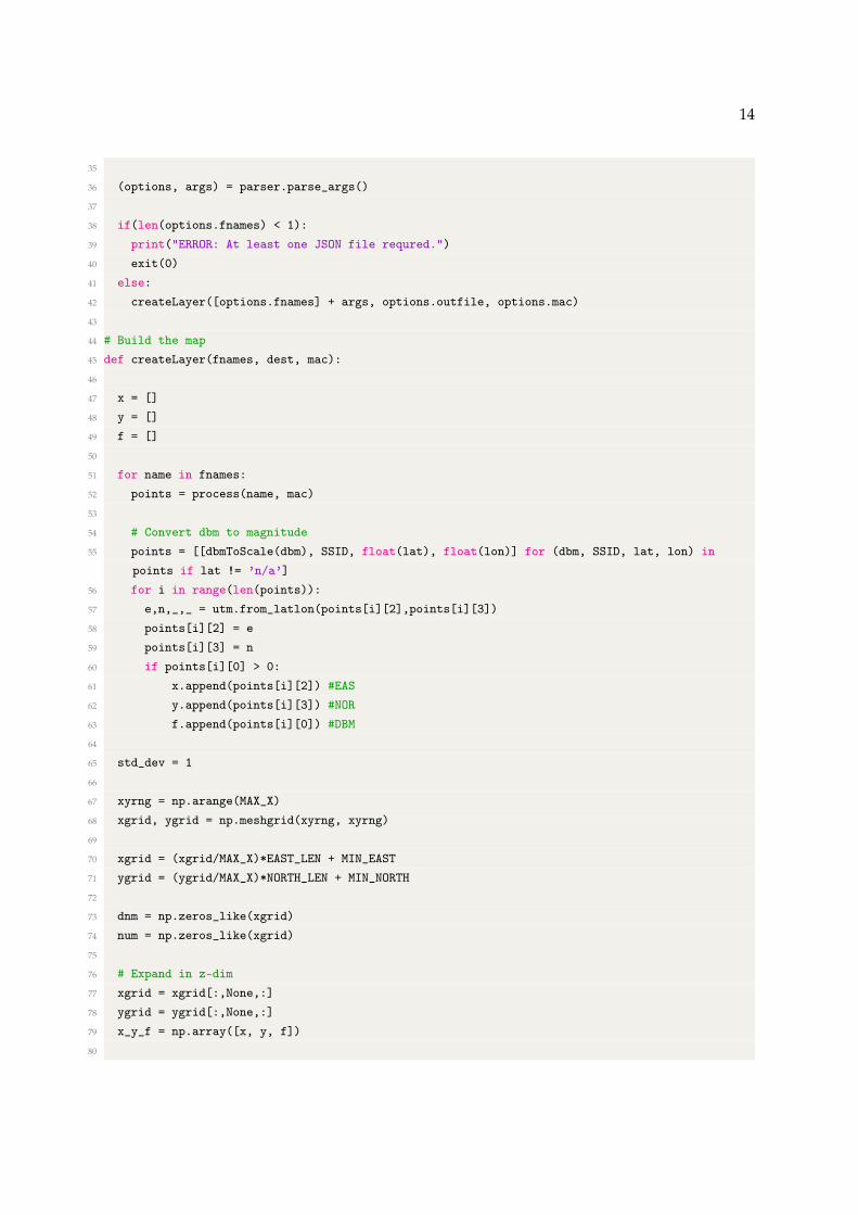
38 if(len(options.fnames) < 1):39 print("ERROR: At least one JSON file requred.")40 exit(0)41 else:42 createLayer([options.fnames] + args, options.outfile, options.mac)43

44 # Build the map45 def createLayer(fnames, dest, mac):46

47 x = []48 y = []49 f = []50

51 for name in fnames:52 points = process(name, mac)53

54 # Convert dbm to magnitude55 points = [[dbmToScale(dbm), SSID, float(lat), float(lon)] for (dbm, SSID, lat, lon) in

points if lat != ’n/a’]56 for i in range(len(points)):57 e,n,_,_ = utm.from_latlon(points[i][2],points[i][3])58 points[i][2] = e59 points[i][3] = n60 if points[i][0] > 0:61 x.append(points[i][2]) #EAS62 y.append(points[i][3]) #NOR63 f.append(points[i][0]) #DBM64

65 std_dev = 166

67 xyrng = np.arange(MAX_X)68 xgrid, ygrid = np.meshgrid(xyrng, xyrng)69

70 xgrid = (xgrid/MAX_X)*EAST_LEN + MIN_EAST71 ygrid = (ygrid/MAX_X)*NORTH_LEN + MIN_NORTH72

73 dnm = np.zeros_like(xgrid)74 num = np.zeros_like(xgrid)75

76 # Expand in z-dim77 xgrid = xgrid[:,None,:]78 ygrid = ygrid[:,None,:]79 x_y_f = np.array([x, y, f])80

15

81 # Create weight with Gaussian PDF82 x = np.array(x_y_f[0])[None,:,None]83 y = np.array(x_y_f[1])[None,:,None]84 f = np.array(x_y_f[2])[None,:,None]85 x_y_f = None86

87 # Write image in chunks in conserve memory88 chunk = len(xgrid)//889 pixels = None90 for i in range(8):91 weight = np.exp(-(np.square((xgrid[chunk*i:chunk*(i+1),] - x)) + \92 np.square((ygrid[chunk*i:chunk*(i+1),] - y))) / (2.0*std_dev**2))93

94 # Build num from weight and sample f95 dnm = np.sum(weight,axis=1)96 num = np.sum(weight * f, axis=1)97 pixels1 = np.where(dnm < 1e-20, None, num/dnm)98 if i != 0:99 pixels = np.concatenate((pixels, pixels1))

100 else:101 pixels = pixels1102

103 # Create Image104 I = Image.new(’RGBA’, (MAX_X, MAX_Y), (255,0,0,0))105 # I.putalpha(32)106 IM = I.load()107 for x in range(MAX_X):108 for y in range(MAX_Y):109 IM[y,x] = color(pixels[x,y])110 if DRAW_DOTS:111 for _, _, e, n in points:112 x, y = en_to_pixel(e, n)113 if 0 <= x < MAX_X and 0 <= y < MAX_Y:114 IM[x,y] = (0,0,0)115

116 if dest:117 I.save("new-public/images/" + dest + ".png", "PNG")118 print("Image written to : new-public/images/" + dest + ".png !")119 else:120 I.save("new-public/images/output.png", "PNG")121 print("Image written to : new-public/images/output.png !")122

123

124 ### Read points and build a ’points’ array of quadruples125 def process(fname, mac):126 points = []127 with open(fname) as f:

16

128 data = json.load(f)129 for item in data[’JsonData’]:130 min_dbm = float(’-inf’)131 for wifi in item[’wifi’]:132 # f0:5c:19:ad:5a:60133 if mac:134 if wifi[’MAC’] == mac:135 min_dbm = float(wifi[’DBM’])136 else:137 if (wifi[’SSID’] == ’eduroam’ and float(wifi[’DBM’]) > min_dbm):138 min_dbm = float(wifi[’DBM’])139

140 points.append((min_dbm, ’eduroam’, item[’Latitude’], item[’Longitude’]))141

142 return points143

144 def color(val):145 stride = 2.5146

147 if val is None:148 return (255,0,0,0)149

150 blue = int(math.cos(val*math.pi/2) * 255)151 green = int(math.sin(val*math.pi) * 255)152 red = int(math.cos((val-1)*(math.pi/2)) * 255)153

154 return (red, green, blue)155

156

157 def sinusoid(a,b,c,d,val):158

159 return (a + b*math.cos(2*math.pi*(c*val + d)))160

161 def pixel_to_en(x,y):162

163 east = (float(x)/MAX_X)*EAST_LEN + MIN_EAST164 north = (float(y)/MAX_Y)*NORTH_LEN + MIN_NORTH165 return east, north166

167 def en_to_pixel(east,north):168

169 x = int(((east-MIN_EAST)/EAST_LEN)*MAX_X)170 y = int(((north-MIN_NORTH)/NORTH_LEN)*MAX_Y)171 return x,y172

173 def distance_squared(x1,y1,x2,y2):174 return (x1-x2)**2 + (y1-y2)**2

17

175

176 def distance(x1,y1,x2,y2):177 return math.sqrt(distance_squared(x1,y1,x2,y2))178

179 def dbmToScale(dbm):180 # Scales dbm so that it is real/positive181 if dbm < -90:182 return 0.0183 elif dbm > -50:184 return 1.0185 else:186 return (dbm + 90)/(40.0)187

188

189 main()