lncs 7335 - a new self-learning algorithm for dynamic

B. Murgante et al. (Eds.): ICCSA 2012, Part III, LNCS 7335, pp. 457–470, 2012. © Springer-Verlag Berlin Heidelberg 2012

A New Self-Learning Algorithm for Dynamic Classification of Water Bodies

Bernd Fichtelmann and Erik Borg

German Aerospace Center, German Remote Sensing Data Center, Kalkhorstweg 53, 17235 Neustrelitz, Germany

{Bernd.Fichtelmann,Erik.Borg}@dlr.de

Abstract. In many applications of remote sensing data land-water masks play an important role. In this context they can be a helpful orientation to distinguish dark areas (e.g. cloud shadows, topographic shadows, burned areas, coniferous forests) and water areas. However, water bodies cannot always be classified exactly on basis of available remote sensing data. This fact can be caused by a variety of different physical and biological factors (e.g. chlorophyll, suspended particles, surface roughness, turbid and shallow water and dynamic of water bodies) as well as atmospheric factors (e.g. haze and clouds). On the other hand the best available static water masks also show deficiencies. These are essentially caused by the fact that land-water masks represent only a temporal snapshot of the water bodies distributed worldwide and therefore these masks cannot reflect their dynamic behavior. This paper presents a dynamic self-learning water masking approach for AATSR remote sensing data in the context of integrating high-quality water masks in processing chains for deriving value-added remote sensing data products. As an advantage to conventional water masking algorithms, the proposed approach operates on basis of a static water mask as data base for deriving an optimized dynamic water mask. Significant research effort was spent to develop and validate a dynamic self-learning algorithm and a processing scheme for operational derivation of actual land-water masks as basis for operational interpretation of remote sensing data. Based on this concept actual activities and perspectives for contributions to operational monitoring systems will be presented.

Keywords: self-learning algorithm, land-water mask, interpretation, remote sensing, cloud cover.

1 Introduction

Satellite Earth observation is a major data source for analyzing environmental subjects. The full-coverage description of status and dynamics of ecological systems is in many cases subject of environmental investigations which deal with sustainable use of natural resources. But in many cases, the actual data base is fragmentary in the required scale [9], [15], [11].

It is not disputed that land-water masks can be helpful additional information for the automated and operational interpretation of remote sensing data. Carroll et al. [3] gives a summary of developments of land-water masks since 1996 and they show

458 B. Fichtelmann and E. Borg

possibilities of additional improvements in global land-water masks. The data can be available in the raster or vector format. The spatial resolution of the data is between 90 m to 25 km. Due to the different requirements of thematic applications and the resulting data management, there are different data sets in different spatial resolution. For example the latest version of the GSHHS data (Global Self-consistent Hierarchical High-resolution Shorelines) of the National Geophysical Data Center [16], released in 2011, is available in a spatial resolution <100 m. At the moment the best available land-water mask is the SRTM Water Body Detection (SWBD) with an accuracy better than 30 m for included water bodies in the geographical region between 54° South and 60° North. Caused by the limited temporal duration (only 11 Days in February 2000) of the SRTM mission, the delivered mission coverage includes data gaps in the data set. Carroll et al. [3] describes according to personal information from the SWDB team in 2006, that the team has tried to infill “these gaps with help of Landsat Geocover data”. However, if the Geocover data were too cloudy, then the appropriate gaps could not be filled.

The preparation of an exact as possible land-water mask aims for example at minimization of inclusion of water pixels in thematic interpretation algorithms for land applications or vice versa. Numerous endeavors exist to improve the quality of global land-water masks, since there is an increasing interest to use such a database in evaluation of remote sensing data.

For this reason the corresponding land-water distribution is an additional information layer of e.g. AATSR and MERIS data delivered to the users. Borg and Fichtelmann [2] suggested a procedure for automatic derivation of data usability of remote sensing data which also includes a water mask in the production process of LANDSAT/ETM+ data.

Available land-water masks are temporal snapshots. Therefore, the most important deficit of these masks is the fact that they cannot reflect the dynamic behavior of water bodies. That means land-water masks are a static information layer.

To counteract possible misinterpretations and to support the land-water classification of remote sensing data, a self-learning procedure was developed that uses available static land-water mask. In a first processing step, the water pixels of the mask will be regarded only as candidates for water. In a second processing step several classification algorithms are used as decision support to classify water. Like before, the water pixels resulting from this second processing step are regarded as possible candidates only. The partial results of the static mask and the different classification mechanisms are fused to an overall result in a third processing step.

Generally, the method is adaptable to other optical sensors. First results of the method applied to AATSR data are shown and discussed.

2 Material and Methods

2.1 Remote Sensing Data

The demonstration of the algorithm is based on multispectral data sets of the Advanced Along-Track Scanning Radiometer (AATSR). This is one of the

A New Self-Learning Algorithm for Dynamic Classification of Water Bodies 459

instruments on board the ENVISAT satellite. The ground resolution of AATSR data at nadir is 1 km. The AATSR-sensor measures reflected and emitted radiation at the centre wavelengths of 0.55 µm, 0.66 µm, 0.87 µm, 1.6 µm, 3.7 µm, 11 µm, and 12 µm. For the investigations the reflectance ρ of bands at 0.55 µm, 0.66 µm, 0.87 µm, 1.6 µm, and for the land surface temperature BT11 the band at 11 μm were used. Additionally two layers with information on latitude and longitude are necessary. The used image sections of complete data sets include all available 512 columns. The number of lines varies between 1000 and 7500. The algorithm was tested on regions of different degrees of difficulties: the Alps with terrain shadow, Scandinavia with inaccuracies of geometry in static mask and the region around Caspian Sea with partly strong changes (desiccation) of water bodies.

2.2 Available Static Land-Water Masks

The generation of a consistent static land-water mask is based on use of different global land-water masks of different spatial resolution and feature accuracy as CIA World-Map or SRTM Water Body Data (SWBD). A short description of global data sets used in these studies is given in the following.

CIA World-Map: As add on of the development software IDL (Interactive Data Language) the 1993 CIA World map database [12], or World DataBank II, is available for operational processing based on USGS map accuracy standards [14].

Fig. 1. CIA world map data include only raw land-water distribution (a) and the result after correction (b) for a part of the Baltic Sea around 60o North

But this add-on includes the disadvantage that the land-water distribution as a whole is not provided with the quality of the coastline information. In some cases continental lakes are not represented as water, in other cases islands are represented as water (Fig. 1a). Based on an object analysis it is possible to combine the information "water" or “land” with the corresponding objects which are embedded by coastlines (Fig. 1b).

SRTM Water Body Data (SWBD): Beside the documentation [13] this data set consists about 12,229 files, covering the Earth between 60° (54°) South and 60°

a) b)


North. For land cells, which are not available in the data set, a data dummy had to be produced. Fig. 2 shows South-America with missing cells in the SWBD data base on the left side and with cells (dummies) infilling these gaps with the information land.

Fig. 2. Available SRTM cells for South America are presented in the left image. In the right image the missing cells were substituted by cells with land information.

3 Dynamically Self-Learning Evaluation Method (DySLEM)

The Dynamically Self-Learning Evaluation Method is based on the use of regional parameters. Therefore, the pre-processing module selects image frames of the complete input-data set. With respect to AATSR these frames have a defined size of 512 x 512 pixels. The data and auxiliary data are used to initiate the DySLEM processor. After finishing of DySLEM a post-processor produces the output product.

3.1 Structure of the Processor

The operational determination of dynamic land-water mask includes three processing steps. The processor structure is shown in Figure 3. In the following a short description of the processor, the used methods, and procedures is given.

Step 1: The work step WS1 generates a regional static land-water mask for selected remote sensing data. For this, the processor uses data of available global static land-water masks. The result is a mask of the percentage water content within image pixel. With regard to the dynamic of water bodies the identified water pixels are regarded only as candidates for water pixels.

Step 2: The work step WS2 includes two different sub-processors for identifying all “candidates” for water. The classification of water is based on spectral properties, relations between different spectral bands or the vegetation index of water bodies. Beside of water the results can include other dark regions.

Step 3: The aim of the work step WS3 is the data fusion of land-water masks processed in WS1 and WS2. On regional level, the data fusion is based at first on the

a) b)


Fig. 3. Processing chain of the processor

water objects reliably identified by part 1 of WS3 (PWS3-1), which were regarded as candidate water pixels in static (WS1) as well as in dynamic masks (WS2). Corresponding water pixels are signed by the fusion processor in a new intermediate mask. Using the spectra of these identified water pixels a mean spectrum is determined. For all other water pixels in the static land-water mask the Fusion Processor initiates sub-processor PWS3-2. This processor tests the derived mean spectrum versus all remaining pixel spectra. Fulfilling this relation, candidate pixels of static mask will be accepted and labelled in the resulting mask and all non-accepted pixels are excluded from further processing. Next the Fusion Processor initiates a third sub-processor PWS3-3. Pixel candidates which are accepted as water in WS2 and are not accepted by sub-processor PSW3-1 will be tested a second time by the sub-processor PSW3-3. Pixels which are defined as water pixels by processor PSW3-3 according to spectral behaviour will be masked as accepted dynamic water and labelled by the Fusion Processor in the final regional dynamic land-water mask.

3.2 Generation of Regional Static Land Water Mask (WS1)

The objective of the first work step (WS1) is the generation of a regional static land water mask lwmss (land water mask, static, section). Therefore, the pre-processing separates AATSR frames of 512 x 512 pixels from the data stream. On basis of corresponding corner coordinates a first map template can be constructed for an area equivalent projection of the AATSR frame into this map [5].The ground resolution of the static land-water mask (lwms) (<100 m) is higher than the ground resolution of


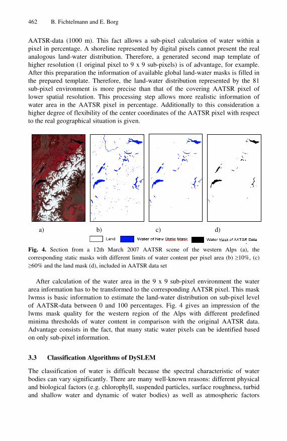
AATSR-data (1000 m). This fact allows a sub-pixel calculation of water within a pixel in percentage. A shoreline represented by digital pixels cannot present the real analogous land-water distribution. Therefore, a generated second map template of higher resolution (1 original pixel to 9 x 9 sub-pixels) is of advantage, for example. After this preparation the information of available global land-water masks is filled in the prepared template. Therefore, the land-water distribution represented by the 81 sub-pixel environment is more precise than that of the covering AATSR pixel of lower spatial resolution. This processing step allows more realistic information of water area in the AATSR pixel in percentage. Additionally to this consideration a higher degree of flexibility of the center coordinates of the AATSR pixel with respect to the real geographical situation is given.

Fig. 4. Section from a 12th March 2007 AATSR scene of the western Alps (a), the corresponding static masks with different limits of water content per pixel area (b) ≥10%, (c) ≥60% and the land mask (d), included in AATSR data set

After calculation of the water area in the 9 x 9 sub-pixel environment the water area information has to be transformed to the corresponding AATSR pixel. This mask lwmss is basic information to estimate the land-water distribution on sub-pixel level of AATSR-data between 0 and 100 percentages. Fig. 4 gives an impression of the lwms mask quality for the western region of the Alps with different predefined minima thresholds of water content in comparison with the original AATSR data. Advantage consists in the fact, that many static water pixels can be identified based on only sub-pixel information.

3.3 Classification Algorithms of DySLEM

The classification of water is difficult because the spectral characteristic of water bodies can vary significantly. There are many well-known reasons: different physical and biological factors (e.g. chlorophyll, suspended particles, surface roughness, turbid and shallow water and dynamic of water bodies) as well as atmospheric factors

a) b) c) d)


(e.g. haze and clouds). Additionally, the observed area of a pixel can consist of an unknown ratio between water and land as discussed before.

Generally the best classification includes always a probability of incompleteness and/or inaccurateness. The pixels classified as dynamic water are considered as candidates. For final decision the self-learning algorithm of the method in WS3 will be used. For these studies two different algorithms for dynamic land-water mask were used to identify all possible different types of water within the section (lwmds).

PWS2-1-Generation of lwmd1s: The bands ρ870, ρ670, ρ550, and ρ1600 are the calibrated reflectance of input-data. The decrease of reflectance ρ with increase of wavelength, the reflectance ρ550 versus the threshold 0.22, and the surface temperature BT11 versus threshold 273 K are to be checked according [6]. The result is mapped into the first land-water mask (lwmd1-AATSR).

Rule (equation 1) for lwmd1s-AATSR:

0 : 1? 273) > (BT110.22) < 550(1600) > 870(

870) > 670(670) > 550(

⋅∧∧∧∧

ρρρρρρρ

. (1)

PWS2-2-Generation of lwmd2s: The second algorithm is based on an unpublished work at the Rutherford Appleton Laboratory by Stevens, A.D. (in [1]). He developed a pixel-based classification scheme using NDVI (Equation 2) and additionally a NDVI-like index NDI2 (Equation 3) for pixel-by-pixel classification based on pre-defined classification criteria. The algorithm was developed to classify clouds. It is also applicable to classify land use and additional classes as water.

)670870/()670870( ρρρρ +−=NDVI . (2)

)550670/()550670(2 ρρρρ +−=NDI . (3)

Stevens uses both indices to define a two-dimensional classification space. Plotting NDVI versus NDI2 for each pixel, different land use types forming different clusters can be identified. When adapting the different surface types including water by the following algorithm, a result lwmd2s comparable with the algorithm before can be derived.

Rule (equation 4) for lwmd2s-AATSR:

0:1?)))25.1/)025.0((2(

)0.0()0.02(())15.0()1.02((

⋅+<∧<∧<∨−<∧<

NDVINDI

NDVINDINDVINDI. (4)

The results of the two masks lwmd1 and lwmd2 are presented in Fig. 5b and c for the same region as in Fig. 4a.

3.4 A Self-Learning Algorithm to Identify Temporal Dynamic of Water Bodies

The different independently operating sub-algorithms of the self-learning algorithm allow the generation of different land-water masks. In consequence, these results can be rule-based selected or merged.


The third work step (WS3) includes three sub-classification processors and a fusion processor. The three masks lwmss, lwmd1s and lwmd2s of the same frame are available.

The aim of the first processing step (PWS3-1) is the determination of stable water pixels. As such all pixels are defined which are included in the static mask as well as identified as water in at least one of the two dynamic land-water masks. Based on static land-water mask lwmss containing the land-water ratio between 0 und 100 percentage, all stable water pixels with more than 60 percentage water content can be determined following the assumption according equation 5.

0:1?60)1211( ⋅>∧=∨= lwmssslwmdslwmd . (5)

All accepted static water pixels are stored by the Fusion Processor in the final matrix lwmd3s. Corresponding water bodies are shown in Figures 5d, 6f, and 7g. The probability of the existence of water is very high in this case.

But it may be that clouds, haze, or ice mask further water pixels in the image data. In case of haze and thin clouds an inclusion of water objects in the resulting mask is useful. In other cases water pixels of the static land-water mask detected by AATSR as dry have to be excluded from further processing. Such a decision is task of PWS3-2.

Based on all n pixels with lwmd3s = 1 the fusion processor calculates generally a regional mean spectrum (all spectral bands i) in preparation of PWS3-2:

nslwmdn

ii /)13(1

== ρρ . (6)

For AATSR sensor only a regional mean temperature was calculated for BT11 on basis of this equation.

Further preparation includes the identification of all pixels of the static mask with a water content ≥ 10% which are not included in lwmd3s. Thus all pixels already marked as stable water will be excluded. After that the Fusion Processor initiates the second step (PWS3-2) of the self-learning algorithm. In case of AATSR data the sub-processor uses the mean surface temperature for testing against the temperature of all water pixels identified by the Fusion Processor.

For improving the results an offset of 5 K is used for (Equation 7). The additionally identified water pixels are encoded with 2 in the resulting mask lwmd3s.

0:2?)5)13(11(11

273111013

⋅+=≤∧>∧≥∧≠

slwmdsBTMEANsBT

sBTlwmssslwmd . (7)

In regions with local shift between static mask and image data results of Equation 7 have shown that vegetation pixels are partly identified as water. Therefore, the inclusion of an additional relation with NDVI is necessary.

As first definite criterion NDVI < -0.04 is used for identifying water pixels which are before identified as candidates of static water. That means Equation 8 allows an


additional adjustment of the results before. The concerning pixels are marked in the resulting mask lwmd3s.

0:2?04.0)5)13(11(11

273111013

⋅−<∧+=≤∧>∧≥∧≠

NDVIslwmdsBTMEANsBT

sBTlwmssslwmd . (8)

In contrast, the second less definite criterion NDVI< +0.15 allows to accept static water pixels of lower probability.

0:3?15.0)5)13(11(11

273111003

⋅+<∧+=≤∧>∧≥∧=

NDVIslwmdsBTMEANsBT

sBTlwmssslwmd . (9)

The results of Equation 8 and Equation 9 shown in Fig. 5d as part of final mask show that pixels of shorelines of different lakes can be identified. Parts of Lake Constance which are masked by haze can be identified as water, too. The principle of the algorithm adapted from Stevens (equation 4) has shown that the restrictions of NDVI are too strong for quality control of static water mask. The use of the relation with NDVI (equation 9) has demanded the additional use of corresponding relations with NDI2, given in equation 10 and equation 11.

0:4?17.087003.0)5501600(

15.02)7)13(11(11

273111003

⋅<∧<−∧−<∧+=≤

∧>∧≥∧=

ρρρNDIslwmdsBTMEANsBT

sBTlwmssslwmd

. (10)

0:5?17.087003.0)5501600(

00.02)7)13(11(11

273111003

⋅<∧<−∧<∧+=≤

∧>∧≥∧=

ρρρNDIslwmdsBTMEANsBT

sBTlwmssslwmd

. (11)

Based on these relations, rivers or shallow water can be effectively identified as accepted static water. After this processing step all pixels of the static water mask with a water area ≥ 10% pixel coverage have been examined. Pixels which satisfy the criteria in any form are included by the Fusion Processor in mask lwmd3s.

Subsequently all pixels of dynamic land-water masks lwmd1s and lwmd2s and which are not marked in the static land-water mask (lwms≥10) will be determined by the Fusion Processor on basis of equation 12. The resulting pixels are marked as “candidate” in the intermediate result mask lwmdis, initiating the next sub-processor.

0:1?121110 ⋅=∧=∧< slwmdslwmdlwmss . (12)

The sub-processor PWS3-3 calculates the second dynamical effect of the mask for dynamic water bodies which are not available in the static water mask. By reason that shadow pixels can likewise fulfil these conditions, an exclusion of these pixels from the final mask is necessary. For shadow pixels the difference of reflectance from band to band is smaller than for water pixels. Therefore for exclusion shadow pixels the


following parameters have to be modified in processing. The following procedure (Equation 13) can be applied [7]:

0:6? 0 1. > 1)=s1600(lwmdi - 1)=870(lwmdis 0.8 > 1)=(lwmdis 870 - 1)=670(lwmdis 0 1. > 1)=(lwmdis 670 - 1)=550(lwmdis

.

(13)

Only pixels which fulfil this relation are encoded in mask lwmd3s with 6 as accepted dynamic water pixel. The work step WS3 will be finished with the DySLEM-output lwmd3s.

After n-runs of DySLEM the n subsets will be integrated into a complete final mask lwmd3 by equation 14.

=n

slwmdlwmd1

33 . (14)

The other masks (lwmss, lwmd1s, lwmd2s) can be combined in the same way.

4 Results

Decisive advantages of the proposed procedure are the identification of difficult classifiable water pixels (see chapter 3.3) and the identification of both "wrong" water pixels caused by data quality problems (e.g. insufficiently accurate geo-correction of the mask) and of water pixels of the static land-water mask which changed their spectral properties after the preparation of the static mask data base (e.g. dried areas).

Based on the following exemplarily discussed results the efficiency and the stability of the proposed procedure will be demonstrated. The selected images include terrain shadows (Alps region), dry or shallow water bodies (region around the Caspian Sea) and qualitative limited static water mask (Scandinavia).

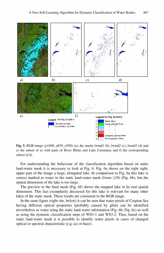
The RGB-image (Fig. 5a) uses the bands ρ1600, ρ870, and ρ550 for a better visibility of dark regions than in Fig. 4a. The visual comparison of RGB-image (Fig. 5a) and final mask (Fig. 5d) shows a good agreement of identified pixels. Fig. 5d demonstrates also that the largest proportion of the water area in the image is identified on basis of both the stable land-water information (compare Fig. 4c) and the dynamic water information. Fig. 5e and 5f show in more detail sections of river Rhine and Lake Constance. The identified pixels of River Rhine (brown colored) are based only on the results of Equation 13. It can also be seen that terrain shadows (Fig. 5c) in the centre of the image can be suppressed (see Fig. 5d).

The comparison of the classification results including terrain shadows (Fig. 5c) with the resulting mask in Fig. 5d shows that the shadow information is eliminated by processing step PWS3-3. In contrast to this, in most cases the cloud shadows in images are no problem for the correct classification because they are already eliminated in processing step WS2.


Fig. 5. RGB-image (ρ1600, ρ870, ρ550) (a), the masks lwmd1 (b), lwmd2 (c), lwmd3 (d) and e) the subset of a) with parts of River Rhine and Lake Constance and f) the corresponding subset of d)

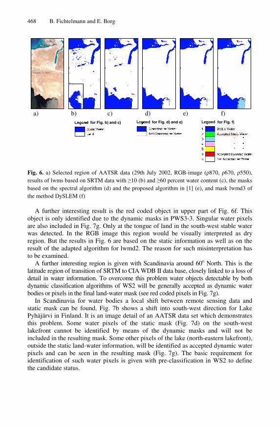
For understanding the behaviour of the classification algorithm based on static land-water mask it is necessary to look at Fig. 6. Fig. 6a shows on the right sight, upper part of the image a large, elongated lake. In comparison to Fig. 6a this lake is correct marked as water in the static land-water mask (lwms ≥10) (Fig. 6b), but the spatial dimension of the lake is too large.

The preview to the final mask (Fig. 6f) shows the mapped lake in its real spatial dimension. This fact exemplarily discussed for this lake is relevant for many other lakes of the static mask. These results are consistent to the RGB image.

In the same figure (right site, below) it can be seen that water pixels of Caspian Sea having different optical properties (probably caused by glint) can be identified nevertheless as water using the static land-water information (Fig. 6b, Fig. 6c) as well as using the dynamic classification steps of WS3-1 and WS3-2. Thus, based on the static land-water mask it is possible to identify water pixels in cases of changed optical or spectral characteristic (e.g. ice or haze).

a) b) c) d)

e) f) for Fig. d) and f)for Fig. b) and c)


Fig. 6. a) Selected region of AATSR data (29th July 2002, RGB-image (ρ870, ρ670, ρ550), results of lwms based on SRTM data with ≥10 (b) and ≥60 percent water content (c), the masks based on the spectral algorithm (d) and the proposed algorithm in [1] (e), and mask lwmd3 of the method DySLEM (f)

A further interesting result is the red coded object in upper part of Fig. 6f. This object is only identified due to the dynamic masks in PWS3-3. Singular water pixels are also included in Fig. 7g. Only at the tongue of land in the south-west stable water was detected. In the RGB image this region would be visually interpreted as dry region. But the results in Fig. 6 are based on the static information as well as on the result of the adapted algorithm for lwmd2. The reason for such misinterpretation has to be examined.

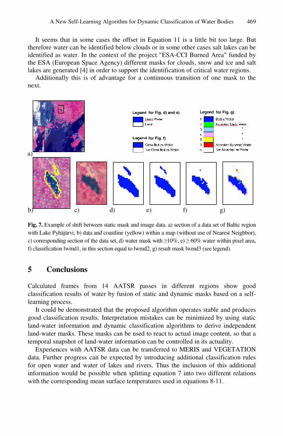
A further interesting region is given with Scandinavia around 60o North. This is the latitude region of transition of SRTM to CIA WDB II data base, closely linked to a loss of detail in water information. To overcome this problem water objects detectable by both dynamic classification algorithms of WS2 will be generally accepted as dynamic water bodies or pixels in the final land-water mask (see red coded pixels in Fig. 7g).

In Scandinavia for water bodies a local shift between remote sensing data and static mask can be found. Fig. 7b shows a shift into south-west direction for Lake Pyhäjärvi in Finland. It is an image detail of an AATSR data set which demonstrates this problem. Some water pixels of the static mask (Fig. 7d) on the south-west lakefront cannot be identified by means of the dynamic masks and will not be included in the resulting mask. Some other pixels of the lake (north-eastern lakefront), outside the static land-water information, will be identified as accepted dynamic water pixels and can be seen in the resulting mask (Fig. 7g). The basic requirement for identification of such water pixels is given with pre-classification in WS2 to define the candidate status.

a) b) c) d) e) f) for Fig. f) for Fig. d) and e)for Fig. b) and c)


It seems that in some cases the offset in Equation 11 is a little bit too large. But therefore water can be identified below clouds or in some other cases salt lakes can be identified as water. In the context of the project "ESA-CCI Burned Area" funded by the ESA (European Space Agency) different masks for clouds, snow and ice and salt lakes are generated [4] in order to support the identification of critical water regions.

Additionally this is of advantage for a continuous transition of one mask to the next.

Fig. 7. Example of shift between static mask and image data. a) section of a data set of Baltic region with Lake Pyhäjärvi, b) data and coastline (yellow) within a map (without use of Nearest Neighbor), c) corresponding section of the data set, d) water mask with ≥10%, e) ≥ 60% water within pixel area, f) classification lwmd1, in this section equal to lwmd2, g) result mask lwmd3 (see legend).

5 Conclusions

Calculated frames from 14 AATSR passes in different regions show good classification results of water by fusion of static and dynamic masks based on a self-learning process.

It could be demonstrated that the proposed algorithm operates stable and produces good classification results. Interpretation mistakes can be minimized by using static land-water information and dynamic classification algorithms to derive independent land-water masks. These masks can be used to react to actual image content, so that a temporal snapshot of land-water information can be controlled in its actuality.

Experiences with AATSR data can be transferred to MERIS and VEGETATION data. Further progress can be expected by introducing additional classification rules for open water and water of lakes and rivers. Thus the inclusion of this additional information would be possible when splitting equation 7 into two different relations with the corresponding mean surface temperatures used in equations 8-11.

a)

b) c) d) e) f) g)

for Fig. g)

for Fig. f)

for Fig. d) and e)


Acknowledgements. This study was made possible by ESA CCI ECV Fire Disturbance project (fire_cci), Nº4000101779/10/I-LG. Furthermore we thank K. Guenther for the constructive discussions and his hints.

References

1. Birks, A.R.: Improvements to the AATSR IPF relating to Land Surface Temperature Retrieval and Cloud Clearing over Land, AATSR Technical Note, Rutherford Appleton Laboratory, Chilton, Didcot, Oxfordshire OX11 0QX, U.K (2007)

2. Borg, E., Fichtelmann, B.: Determination of the usability of remote sensing data- EP 1591961 B1 (2005)

3. Carroll, M.L., Townshend, J.R., DiMiceli, C.M., Noojipady, P., Sohlberg, R.A.: A new global raster water mask at 250 m resolution. Int. J. of Digital Earth 2, 291–308 (2009)

4. ESA CCI ECV Fire Disturbance (fire_cci), N°4000101779/10/I-LG 5. Fichtelmann, B., Borg, E., Kriegel, M.: Verfahren zur operationellen Bereitstellung von

Zusatzdaten für die automatische Fernerkundungsdatenverarbeitung. In: 23rd AGIT Symposium Angewandte Geoinformatik 2011, Strobl, Blaschke, Griesebner, Salzburg, pp. 12–20 (2011)

6. Günther, K.P.: ESA-CCI-Burnt Area Pre-Processing, Kick-off Meeting. ESA-CCI Burnt Area Pre–Processing (2010a)

7. Günther, K.P.: Private communication (2010b) 8. Haas, E.M., Bartholomé, E., Combal, B.: Time series analysis of optical remote sensing

data for the mapping of temporary surface water bodies in sub-Saharan western Africa. J. Hydrology 370, 52–63 (2009)

9. Justice, C., Giglio, L., Korontzi, S., Owens, J., Morisette, J., Roy, D., Descloitres, J., Alleaume, S., Petitcolin, F., Kaufman, Y.: The MODIS fire products. Remote Sensing of Environment 83(1&2), 244–262 (2002)

10. Landsat 7 User Handbook, http://landsathandbook.gsfc.nasa.gov/data_ properties/

11. Lehner, B., Doll, P.: Development and validation of a global database of lakes, reservoirs, and wetlands. Journal of Hydrology 296, 1–22 (2004)

12. Pape, D.: CIA World DataBank II, http://www.evl.uic.edu/pape/data/WDB/ (last modified, 2004)

13. USGS: Documentation for the Shuttle Radar Topography Mission (SRTM) Water Body Data Files, http://dds.cr.usgs.gov/srtm/version2_1/SWBD/SWBD_ Documentation/Readme_SRTM_Water_Body_Data.pdf

14. USGS (U.S. Geological Survey): Map Accuracy Standards, USGS Fact Sheet, pp. 171–199 (1999), http://erg.usgs.gov/isb/pubs/factsheets/fs17199.pdf

15. Wan, Z., Zhang, Y., Zhang, Q., Li, Z.: Validation of the land-surface temperature products retrieved from Terra Moderate Resolution Imaging Spectroradiometer data. Remote Sensing of Environment 83(1&2), 163–180 (2002)

16. Wessel, P., Smith, W.H.F.: A global, self-consistent, hierarchical, high-resolution shoreline database. J. Geophys. Res. 101(B4), 8741–8743 (1996)

lncs 7335 - a new self-learning algorithm for dynamic

Documents