lncs 7577 - towards optimal design of time and color ...mx.nthu.edu.tw/~tsunghan/papers/conference...

Towards Optimal Design

of Time and Color Multiplexing Codes

Tsung-Han Chan1,2, Kui Jia1, Eliot Wycoff1, Chong-Yung Chi2, and Yi Ma3,4

1 Advanced Digital Sciences Center, Singapore2 Inst. Communications Eng., National Tsing Hua University, Taiwan

3 Microsoft Research Asia, Beijing, China4 Dept. Elect. and Computer Eng., University of Illinois at Urbana-Champaign

{Th.chan,Chris.jia,Eliot.wycoff}@adsc.com.sg, [email protected]

Abstract. Multiplexed illumination has been proved to be valuable andbeneficial, in terms of noise reduction, in wide applications of computervision and graphics, provided that the limitations of photon noise andsaturation are properly tackled. Existing optimal multiplexing codes, inthe sense of maximum signal-to-noise ratio (SNR), are primarily designedfor time multiplexing, but they only apply to a multiplexing system re-quiring the number of measurements (M) equal to the number of illu-mination sources (N). In this paper, we formulate a general code designproblem, where M ≥ N , for time and color multiplexing, and develop asequential semi-definite programming to deal with the formulated opti-mization problem. The proposed formulation and method can be readilyspecialized to time multiplexing, thereby making such optimized codeshave a much broader application. Computer simulations will discover themain merit of the method— a significant boost of SNR as M increases.Experiments will also be presented to demonstrate the effectiveness andsuperiority of the method in object illumination.

Keywords: Multiplexing codes, maximum SNR, convex optimization.

1 Introduction

Optical multiplexing can be tracked back to the late 70s in the field of spec-trometry [1], where a single detector simultaneously receives signals from differ-ent spectral bands which are specifically encoded. The goal of multiplexing is toimprove signal-to-noise ratio (SNR) of the demultiplexed, single spectral bandsignals. An analogous multiplexing concept has been brought into the domain ofcomputer vision and graphics by Schechner et al. in 2003 [2], where they illumi-nated objects by multiple sources from different directions and computationallydemultiplexed the received images, attempting to acquire high-SNR, single-lightsource images. Such a multiplexing scheme was afterwards employed in applica-tions, such as scene recovery [3], object relighting [4], fluorescence unmixing [5]and photometric stereo [6–8], and has been proved to improve SNR.

The SNR boost of single-light source images is anticipated to have a pro-found and immediate impact on the successes in computer vision applications.

A. Fitzgibbon et al. (Eds.): ECCV 2012, Part VI, LNCS 7577, pp. 485–498, 2012.c© Springer-Verlag Berlin Heidelberg 2012

486 T.-H. Chan et al.

For instance, in face recognition system [9], gathering face training images underarbitrary illuminations via multiplexing scheme would result in noise reductionand subsequently improve the recognition rate. In photometric stereo [6–8], esti-mating the surface normals of objects from the multiplexing-applied, single-lightsource images can substantially aid in object recognition and 3-D modeling. Theabove advantages are expected when there is only sensor noise involved. Whenthe photon noise comes into play, multiplexing multiple light sources may be-come counterproductive [10]. Present efforts for designing multiplexing codes inthe presence of both sensor noise and photon noise include the works in [10–12],but they are limited to time multiplexing system where the number of mea-surements (M) equals the number of illumination sources (N). Some questionsmay arise: How to design the multiplexing codes for the system not only ap-plying time multiplexing but also color multiplexing? What we can gain fromthe multiplexing if the number of measurements M is more than the number ofillumination sources N?

Indeed, some existing works have utilized time and color multiplexing forvarious purposes [4, 7, 13, 14], but there is not much information on how thetime and color multiplexing codes were designed. In this paper, we investigatethe possibility of designing optimal time and color multiplexing codes, withM ≥ N , for achieving maximum SNR in the demultiplexed images. We firstformulate the code design problem as a constrained optimization problem, andit takes into account the presence of sensor noise and photon noise, as well as thesaturation issue [11]. Since the formulated problem is non-convex, we propose touse a sequential convex programming to approximate the problem, where eachsubproblem is formulated as a semi-definite program and thus can be solved byany convex optimization solver. The proposed formulation and algorithm can bereadily specialized to time multiplexing, thereby making such optimized codeshave a much broader application. Simulations will discover the merits of ourapproach— a significant SNR boost when M increases, and requirement of 1/Kmeasurements in time and color multiplexing for achieving equal performancewhen using time multiplexing, where K denotes the number of color channels;e.g., K = 3 for RGB color camera. Experiments are presented to demonstratethe effectiveness and superiority of the proposed approach in object illumination.

2 Background of Time Multiplexing

We briefly review the background of time multiplexing and some related worksin this section. To start with, let us consider a scenario that a static object withLambertian surfaces is illuminated by multiple, sayN , diverse single light sourcesusing time-multiplexed scheme, and each light source has its own direction fromwhich the light source illuminates a surface patch of the object. Assuming thereare N distinct multiplexed illuminations in total, the captured intensity valueat pixel n can be represented by a linear superposition model:

x[n] = As[n] + v[n], n = 1, ..., L, (1)

Towards Optimal Design of Time and Color Multiplexing Codes 487

where x[n] ∈ RN is a vector containing the captured light intensity for N dif-

ferent multiplexed illuminations at pixel n, A ∈ RN×N is a time multiplexing

matrix, s[n] = [s1[n], ..., sN [n]]T denotes a vector comprising intensities of thereflected light at the nth pixel, under different N single lighting conditions,v[n] ∈ R

N is the measurement noise, and L is the total number of image pix-els. The 1-dimensional pixel index n results from a vector transformation of2-dimensional image coordinate.

Time multiplexing in (1) uses non-switching strategy, where the elements ofthe matrix A are from 0 to 1, not restricted to 0 or 1; i.e., 0 � vec(A) � 1NN ,where� denotes componentwise inequality for vectors or linear matrix inequalityfor matrices, vec(·) denotes vectorization operator, 1N is N -dimensional all-one vector, and 0 is all-zero vector of proper dimension. The extreme values0 and 1 stand for the corresponding light source being completely turned offand turned on, respectively. The values of {s[n]}Ln=1 depend on object and lightsource relative position, orientation and visibility. In addition, the noise v[n] isassumed to be independent and identically distributed (i.i.d.), zero mean, withcovariance matrix satisfying the affine noise model [4, 15]:

ΣP = (σ2 + Pρ2)IN , (2)

where σ2 denotes the variance of the signal-independent sensor noise, ρ2 denotesthe variance of signal-dependent photon noise, IN is N ×N identity matrix, andP is total energy of the activated light sources at each measurement. The valueof P has a direct connection to the time multiplexing matrix A, indicating themultiplexing power used in each measurement is equal to P ; i.e., A1N = P1N .

A solution to recover the pixel values under various single-light source il-luminations s[n], n = 1, ..., L is to multiply A−1 to the multiplexed imagesx[n], n = 1, ..., L:

s[n] = A−1x[n] = s[n] +A−1v[n], n = 1, ..., L. (3)

From (3), it is obvious that the single-light source illumination s[n] can be esti-mated subject to some noise contamination A−1v[n]. A question arises: Couldsomeone make use of A so as to demultiplex high quality s[n], or to minimizethe effect of noise A−1v[n] in s[n]. This is exactly the primary goal of the mul-tiplexing, which attempts to devise the time multiplexing matrix A such thatthe estimated single-light source illumination s[n] has maximum signal-to-noiseratio (SNR) [11], or equivalently,

{A�, P �} = arg minA∈RN×N ,P∈R

Tr((ATΣ−1P A)−1)

s.t. 0 � vec(A) � 1NN , A1N = P1N ,(4)

where Tr(·) is the trace operator. As compared to the scenario of single-sourceacquisition; i.e., A = IN , the SNR gain of time multiplexing can be easily com-puted as

Gt =

√

Tr(Σ1)

Tr(((A�)TΣ−1P�A�)−1)

, (5)


where Σ1 is given by (2) with setting P = 1. The SNR gain Gt can also be calledas time multiplexing gain.

2.1 Related Works

In the following, we categorize previously related works based on conditionsunder which the methods for handling problem (4) were developed.

Absence of Photon Noise: Optical multiplexing technique was first investi-gated in the field of spectrometry [1]. The optimal multiplexing codes for problem(4) has been shown to be S-matrix [1,2,4] when the photon noise is absent; i.e.,ρ2 = 0. The S-matrix can be readily constructed based on Hadamard codes oflengthN+1 for someN such that (N+1)/4 is an integer. Hadamard multiplexingis switch multiplexed method, which completely turns on P � = (N + 1)/2 lightsources at each measurement. Using Hadamard multiplexing, the time multiplex-ing gain is Gt = (N+1)/(2

√N) [1]. Clearly, the more the number of illumination

sources N , the more image quality we can gain using multiplexing.

Presence of Photon Noise: When photon noise comes into play, Hadamardmultiplexing is not optimal anymore [6]. Mutting [10] looked into the effect ofphoton noise to Hadamard multiplexing, and derived new multiplexing codes,based on two-level autocorrelation sequences. These multiplexing codes haveshown their advantages when there are photon noise, but they are only availablefor a very limit set of N and for limit range of noise variances {σ2, ρ2}. Thus,Ratner et al. [11] constructed new time multiplexing codes for any N and noisevariances {σ2, ρ2}. They dealt with problem (4) for a given P using the pro-jected gradient method, which may easily get stuck in the local optima duringthe solution search. Hence, they also devise a higher level optimization procedurefor the method to escape from local optima [11]. After collecting all the optimalobjective values of problem (4) for all the P ’s, the optimal P � was then selectedas the one with minimum objective value.

Saturation: Another issue encountered in illumination multiplexing is satura-tion, and it may occur when the object is illuminated by numerous light sources.When the captured image intensity is saturated, meaning that the linear super-position model (1) is violated, one should either reduce the exposure time ordecrease the total energy P for each measurement. [2, 4] has proved that thelatter is better than the former. Thus, to counter saturation issue, Ratner et al.have added a constraint:

P ≤ Psat, (6)

where Psat is the threshold beyond which the captured image gets saturated.Despite the success of the above methods, the present time multiplexing codes

are limited to time multiplexing and the determined, multiplexing system (orA ∈ R

N×N is square). Some interesting questions may arise: Can the codedesign problem for time multiplexing be extended to that for time and colormultiplexing? What if the multiplexing system can allow to capture more numberof measurements? In the next section, we will formulate a maximum-SNR code


design problem for time and color multiplexing, where the multiplexing matrix isnot limited to be square. Some advantages of employing, over-determined, timeand color multiplexing system will be discovered and discussed therein.

3 Time and Color Multiplexing

Time and color multiplexing has been utilized for relighting [4], multi-spectralimaging [13], and capturing varying illumination conditions [7, 14], but none ofthem specifically elaborate how to optimally devise the codes for time and colormultiplexing. In this section, we introduce the model of time and color multiplex-ing, and present how the codes for time and color multiplexing can be designedin a near-optimal way. As reported in [14], the captured time-multiplexing im-ages of a static Lambertian object at RGB channels should fulfill the followinglinear superposition model:

xc[n] = αc[n]Acs[n] + vc[n], n = 1, . . . , L, c ∈ {r, g, b} (7)

where xr[n],xg[n],xb[n] ∈ RM denote M -time multiplexed image intensity at

pixel n, recorded via red, green, and blue channels, respectively, αr[n], αg[n], αb[n]∈ R represent the illumination-independent, normalized RGB intensities of thematerial at image pixel n, satisfying αr[n] + αg[n] + αb[n] = 1, n = 1, ..., L,Ar,Ag,Ab ∈ R

M×N are the time-multiplexing matrices for red, green, andblue channels, respectively, s[n] ∈ R

N corresponds to various single-light sourceilluminations at pixel n, and vr [n],vg[n],vb[n] ∈ R

M denote the i.i.d. noisemeasured in RGB channels, respectively. The noise covariance matrices for RGBchannels are usually diverse, depending on specification of the color camera used;i.e., Σc

P = (σ2c +Pρ2c)IM , c ∈ {r, g, b}. Here, the number of time multiplexing M

can be different from the number of illumination sources N . Also, the materialcolors and the noise covariance matrices can be practically acquired in cameracalibration phase, and they are assumed to be known herein. The details of howto estimate those parameters can be referred to Section 5.1.

We first reformulate the model (7). Moving the effects of material colorsαr[n], αg[n], αb[n], n = 1, ..., L into noise, and staking RGB counterparts asa column vector, we obtain

y[n] �

⎡

⎣

xr [n]/αr[n]xg[n]/αg[n]xb[n]/αb[n]

⎤

⎦ =

⎡

⎣

Ar

Ag

Ab

⎤

⎦ s[n] +

⎡

⎣

vr[n]/αr[n]vg[n]/αg[n]vb[n]/αb[n]

⎤

⎦ ∈ R3M (8)

= Fs[n] +w[n], n = 1, ..., L, (9)

where F = [ ATr ,A

Tg ,A

Tb ]T ∈ R

3M×N is the time and color multiplexing matrix,

and w[n] = [ v[n]Tr /αr[n],v[n]Tg /αg[n],v[n]

Tb /αb[n] ]

T ∈ R3M is the noise having

block diagonal covariance matrix

ΛP = Bdiag

(

L∑

n=1

ΣrP

α2r[n]L

,L∑

n=1

ΣgP

α2g[n]L

,L∑

n=1

ΣbP

α2b [n]L

)

∈ R3M×3M , (10)


thanks to i.i.d. property of the noise. Here, Bdiag(C1, ...,CN ) denotes a blockdiagonal matrix with the diagonal blocks equal to C1, ...,CN . The structure in(10) is for ease of presentation, and any correlation across RGB channels causedby Bayer filter and color interpolation will not change the optimization procedure(to be presented in Section 3.1) and the optimality of the yielded solution.

Assuming that 3M ≥ N , the unique recovery of single-source illuminations[n] from y[n] can be written as

s[n] = GTy[n] = s[n] +GTw[n], n = 1, ..., L, (11)

where G ∈ R3M×N is a demultiplexing matrix such that GTF = IN . Unlike the

case of 3M = N , whereG can be trivially determined as F−1, we herein considerG is unknown and to be designed. Hence, the time and color multiplexing is tojointly devise F and G such that the SNR of s[n] is maximum, which turns outto be equivalent to minimizing the noise power subject to all the constraintsconsidered in (4):

minF,G∈R3M×N ,P∈R

Tr(GTΛPG)

s.t. GTF = IN , 0 � vec(F) � 13MN , F1N = P13M .(12)

By the Lagrangian multiplier method [16], we can obtain the a closed-formsolution G for the above problem, in terms of F and P , as follows:

G� = Λ−1P F(FTΛ−1

P F)−1. (13)

The details of how we derive (13) can be found in the Supplementary Material(SM)1. Substituting (13) into (12) yields

{F�, P �} = arg minF∈R3M×N ,P∈R

Tr((FTΛ−1P F)−1)

s.t. 0 � vec(F) � 13MN , F1N = P13M .(14)

In comparison to straightforward time and color multiplexing; i.e., 3M = N andF = IN , the gain of optimal time and color multiplexing can be defined as

Gtc =

√

Tr(Λ1)

Tr(((F�)TΛ−1P�F�)−1)

, (15)

where Λ1 is the noise covariance given by (10) with P = 1.The objective function of problem (14) is highly non-convex. Directly handling

this problem with any non-linear programming method could suffer from risk oflocal optimality. Though one may use Ratner’s method [11,12] to tackle problem(14), it is limited to the case of square multiplexing matrix 3M = N and ΛP =βI3M for any β > 0. In what follows, we propose to handle problem (14) ofany 3M ≥ N and ΛP by sequential convex programming (SCP), where eachsubproblem involved in SCP is in form of semi-definite programming (SDP) andhence can be readily solved by convex optimization solvers [17].

1 The SM can be downloaded athttp://web.adsc.com.sg/perception/publications.html.

http://web.adsc.com.sg/perception/publications.html


3.1 Design of Time and Color Multiplexing Codes

To alleviate difficulties in solving problem (14), we adopt a divide-and-conquerstrategy. We first deal with problem (14) by SCP with P fixed, and then findthe optimal P by exhaustive search. Now, suppose that the variable P is fixedto a constant P . Then, problem (14) can be reformulated into its equivalent,alternative form:

minF∈R

3M×N ,H∈RN×N

Tr(H)

s.t. 0 � vec(F) � 13MN , F1N = P13M , H � (FTΛ−1PF)−1,

(16)

where the last constraint, linear matrix inequality, can be further rewritten, viaSchur’s complement [18, Th. 7.7.6, p. 472], as

[

H ININ FTΛ−1

PF

]

� 0. (17)

By letting U = FTΛ−1PF, we can write problem (16) as

minF∈R

3M×N ,H,U∈RN×N

Tr(H)

s.t. 0 � vec(F) � 13MN , F1N = P13M , (18a)

U = FTΛ−1PF, (18b)

[

H ININ U

]

� 0. (18c)

Solving problem (18) is difficult, due to non-convexity of (18b). Next, we seekfor local optimization methods that approximate (18b) using first-order Taylorseries, so as to make problem (18) able to be solved by a sequence of convexproblems. Applying Newton’s method [19] to the quadratic matrix equationQ(F) = U − FTΛ−1

PF = 0, where Q : R

N×N �→ RN×N is a continuously

differentiable function, will have the following recurrence

given F0 (initial guess of F), (19a)

U− FTkΛ

−1PFk = FT

kΛ−1PΔF+ΔFTΛ−1

PFk, (19b)

Fk+1 = Fk +ΔF, k = 0, 1, 2, ... (19c)

where ΔF denotes a small change in F, and Fk denotes the estimate of F atiteration k. The details of how we derive (19) is provided in the SM1. Since thenewly updated Fk+1 should be feasible to (18), Fk+ΔF should also fulfill (18a).By replacing the equality constraint (18b) with (19b), at each iteration k, wecan obtain the following SDP formulation:

minΔF∈R

3M×N ,H,U∈RN×N

Tr(H)

s.t. 0 � vec(Fk +ΔF) � 13MN , (Fk +ΔF)1N = P13M ,

U− FTkΛ

−1PFk = FT

kΛ−1PΔF+ΔFTΛ−1

PFk,

H,U satisfy (18c).

(20)


The above SDP problem can be efficiently solved by any convex optimizationsolvers [17]. Note that problem (18) is now handled by a sequence of SDPsgiven by (20). In each iteration k, problem (20) is thought of as a local, linearapproximation to problem (18). Once ΔF is obtained at the iteration k, we willupdate Fk+1 by (19c), and continue to solve problem (20) for k := k + 1.

Since SCP is a local approximation, using the iterative SCP (20) for solvingproblem (18) may converge to local minima. To reduce the risk of local optima,we empirically impose a penalty term to the objective function, which amountsto the maximum of the off-diagonal elements of the matrix U; i.e.,

D(U) = maxi�=j

uij , (21)

where uij is the (i, j)th element of U. The idea is motivated by the fact thatminimizing the objective function Tr(U−1) in (14) suffices maximizing Tr(U), orminimizing D(U), due to the properties uij ≥ 0, ∀i, j,∑ uij = P 21T

3MΛ−1P13M ,

and U � 0, inferred from (18a)-(18b). The complete SCP for problem (18) issummarized in Algorithm 1. The initial F0 should be feasible— the elementsof F0 are randomly generated following uniform distribution over [0, 1], and arenormalized to satisfy (18a). The weight of the penalty function λ is empirically

set to 2N/(3 PM). The iteration procedure will stop when the relative change inobjective function is smaller than a preset threshold. A convenient implementa-tion of Algorithm 1 using CVX [17] is provided in the SM1.

Algorithm 1. Sequential convex programming for problem (18).

input : total energy of the multiplexing P , the noise covariance matrix ΛP

given by (10), initial multiplexing codes F0, λ = 2N/(3 PM) anditeration number k = 0.

while not converged dosolve the linearized convex problem

{ΔF�,H�,U�} = arg minΔF,H,U

Tr(H) + λD(U) s.t. all constraints in (20);

update Fk+1 = Fk +ΔF� and k := k + 1;

end

output: solution F( P ) = Fk and optimal value J( P ) = Tr(H�) to problem (16).

The remaining problem is to determine the optimal total energy of the ac-tivated light sources P . Once the optimal value J( P ) for P = 2, 3, ..., Psat areobtained by Algorithm 1, where setting Psat given by (6) as an upper bound is toaccount for saturation problem in multiplexing, the time and color multiplexingmatrix F to problem (14) can be found by F� = F(P �) for

P � = minP=2,3,..,Psat

J( P ). (22)


3.2 Application of Algorithm 1 to Time Multiplexing

The methodology shown in the above subsection can also be applied to timemultiplexing. Recall the time multiplexing model (1), where A becomes M ×Ninstead of N ×N conventionally addressed in the previous works [1,2,4,10,11].Following the similar derivations in (11), (12), (13) and (14), the design of suchA ∈ R

M×N is to solve the optimization problem

{A�, P �} = arg minA∈RM×N ,P∈R

Tr((ATΣ−1P A)−1)

s.t. 0 � vec(A) � 1MN , A1N = P1M .(23)

Since problem (23) has a similar structure as (14), following Section 3.1, one canapply Algorithm 1 to solve problem (23); see the SM1 for details.

4 Computer Simulations

The performance of the proposed code design algorithm, in terms of multiplexinggain, will be demonstrated, for time multiplexing, as well as time and color mul-tiplexing in this section. The purpose of showing results with time multiplexingis to make a baseline comparison with the existing algorithms [11, 12].

4.1 Time Multiplexing

There are N = 24 distinct illuminations, and M = 24, 48, 72 measurementsallowed to be captured by using time multiplexing. Two noise parameters givenby (2) are set to σ2 = 1.5 and ρ2 = 0. Figure 1(a) shows the comparableperformance of the proposed method (i.e., Alg1) to Ratner’s method [11] forM = 24. Next, we further examine the performance of the proposed methodto various number of measurements. Since Ratner’s method was developed fordetermined multiplexing system M = N = 24, we repeat Ratner’s optimal24× 24 multiplexing matrix twice and three times for M = 48, 72, respectively.As shown in Figure 1(b), the performance improvement of the proposed methodover Ratner’s method can be obviously seen as M > N , regardless of the valueof P . This immediately suggests that if someone demands a high-quality imageunder single lighting condition, the solution for that is to acquire more numberof measurements using the proposed multiplexing codes.

4.2 Time and Color Multiplexing

We consider the time and color multiplexing where there are N = 24 disparateilluminations and M = 8, 16, 24 number of RGB multiplexed images. Some noiseparameters in ΛP in (10) are set to σ2

r = 1.5, σ2g = 0.9σ2

r , σ2b = 2σ2

r , andρ2c = σ2

cχ2, c ∈ {r, g, b}, where χ2 denotes the common ratio of the sensor

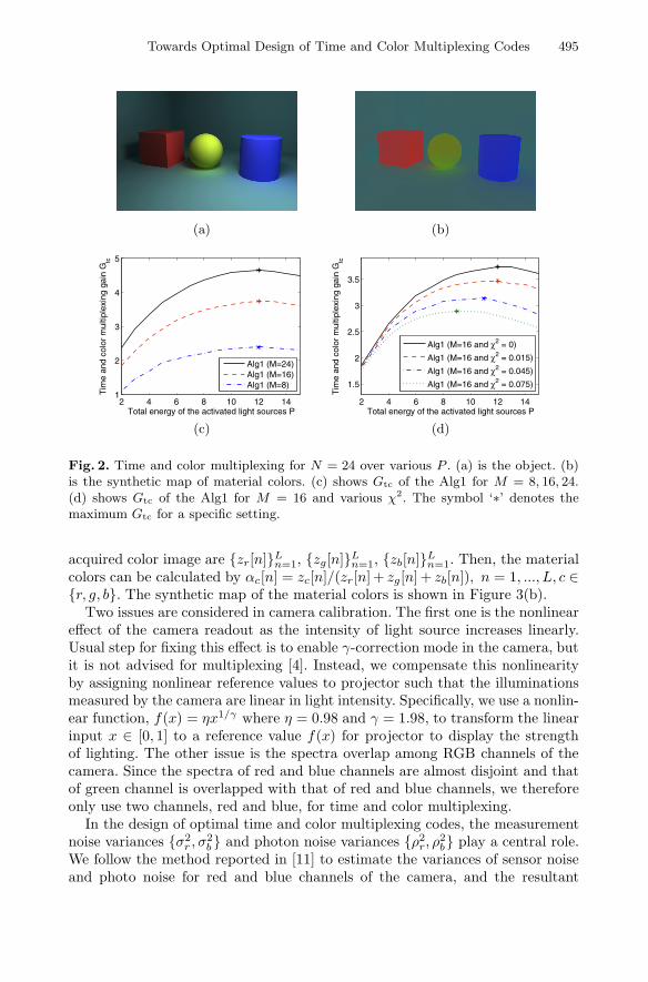
noise power and photon noise power for RGB channels. Figure 2(a) shows theobject to be illuminated. Figure 2(b) is the synthetic map of material colors


2 4 6 8 10 12 141

1.5

2

2.5

Total energy of the activated light sources P

Tim

e m

ultip

lexi

ng g

ain

Gt

Alg1Ratner’s method [11]

(a)

2 4 6 8 10 12 14

0.5

1

1.5

2

2.5

3

3.5

4

4.5


Tim

e m

ultip

lexi

ng g

ain

Gt

Alg1 (M=72)Ratner’s method (M=72)Alg1 (M=48)Ratner’s method (M=48)Alg1 (M=24)Ratner’s method (M=24)

(b)

Fig. 1. Time multiplexing for N = 24 over various P . (a) shows Gt of the proposedmethod (Alg1) and Ratner’s method for M = 24. (b) shows Gt of the Alg1 and Ratner’smethod for M = 24, 48, 72, where ‘∗’ denotes the maximum Gt for a specific M .

of the object. Figure 2(c) shows the time and color multiplexing gain of theproposed Alg1 for M = 8, 16, 24 in the absence of photon noise; i.e., χ2 = 0. Themultiplexing gain improves as the number of measurements M increases. Whilethis observation is similar to time multiplexing shown in Figure 1(b), to maintainthe equal multiplexing gain, the number of measurements required by time andcolor multiplexing is less than time multiplexing by a factor of 3, thanks to threeRGB channels utilized for multiplexing. Moreover, the impact of photon noiseon the time and color multiplexing is also evaluated in Figure 2(d). It can beseen that the optimal total energy of the activated light sources P � may decreasewhen the photon noise goes up, or χ2 increases. This directly reflects the factthat multiplexing more light sources P results in superposition of more photonnoise, and the optimal P should be pulled back in the presence of photon noise.

5 Experiments

We demonstrate the effectiveness of the proposed time and color multiplexingmethod by object illumination. A PC-controlled BENQMX761 projector createdpatterns of N = 24 light patches on a white diffuse wall corner. Lights reflectedby these patches acted as separate light sources illuminating the placed object—pink piglet, shown in Figure 3(a). A camera FUJINON FL2G13S2C-C was usedto capture the multiplexed images, and its exposure time and amplifier gainwere set to 150 msec and 0 dB, respectively. The experiment setup, illuminationpatterns, and some more results are provided in the SM1.

5.1 Material Colors, Calibration and Noise Estimation

A pre-scan of the object under white light condition is required for estimationof the RGB material colors of the object. Suppose that the RGB values of the


(a) (b)

2 4 6 8 10 12 141

2

3

4

5


Tim

e an

d co

lor

mul

tiple

xing

gai

n G

tc

Alg1 (M=24)Alg1 (M=16)Alg1 (M=8)

(c)

2 4 6 8 10 12 14

1.5

2

2.5

3

3.5


Tim

e an

d co

lor

mul

tiple

xing

gai

n G

tc

Alg1 (M=16 and χ2 = 0)

Alg1 (M=16 and χ2 = 0.015)

Alg1 (M=16 and χ2 = 0.045)

Alg1 (M=16 and χ2 = 0.075)

(d)

Fig. 2. Time and color multiplexing for N = 24 over various P . (a) is the object. (b)is the synthetic map of material colors. (c) shows Gtc of the Alg1 for M = 8, 16, 24.(d) shows Gtc of the Alg1 for M = 16 and various χ2. The symbol ‘∗’ denotes themaximum Gtc for a specific setting.

acquired color image are {zr[n]}Ln=1, {zg[n]}Ln=1, {zb[n]}Ln=1. Then, the materialcolors can be calculated by αc[n] = zc[n]/(zr[n] + zg[n] + zb[n]), n = 1, ..., L, c ∈{r, g, b}. The synthetic map of the material colors is shown in Figure 3(b).

Two issues are considered in camera calibration. The first one is the nonlineareffect of the camera readout as the intensity of light source increases linearly.Usual step for fixing this effect is to enable γ-correction mode in the camera, butit is not advised for multiplexing [4]. Instead, we compensate this nonlinearityby assigning nonlinear reference values to projector such that the illuminationsmeasured by the camera are linear in light intensity. Specifically, we use a nonlin-ear function, f(x) = ηx1/γ where η = 0.98 and γ = 1.98, to transform the linearinput x ∈ [0, 1] to a reference value f(x) for projector to display the strengthof lighting. The other issue is the spectra overlap among RGB channels of thecamera. Since the spectra of red and blue channels are almost disjoint and thatof green channel is overlapped with that of red and blue channels, we thereforeonly use two channels, red and blue, for time and color multiplexing.

In the design of optimal time and color multiplexing codes, the measurementnoise variances {σ2

r , σ2b} and photon noise variances {ρ2r, ρ2b} play a central role.

We follow the method reported in [11] to estimate the variances of sensor noiseand photo noise for red and blue channels of the camera, and the resultant


(a) (b)

2 4 6 8 10 12 14

0.5

1

1.5

2

2.5

3

3.5


Tim

e an

d co

lor

mul

tiple

xing

gai

n G

tc

Alg 1 (M=48, Dual Channels)Alg 1 (M=24, Dual Channels)Alg 1 (M=12, Dual Channels)

(c) (d)

(e) (f)

(g) (h)

Fig. 3. Experimental results of time and color multiplexing for object illumination.(a) is the object to be illuminated. (b) is the synthetic map of material colors{αr[n], αg [n], αb[n]}Ln=1. (c) presents the time and color multiplexing gain Gtc forM = 12, 24, 48, and ‘∗’ denotes the maximum Gtc for a specific M . (d) representsone of the multiplexed images. (e) is the 12th demultiplexed image via trivial illu-mination M = 12,F = I24. (f)-(h) correspond to the 12th single-light source imagesdemultiplexed from 12, 24, 48 time and color multiplexed images, respectively.


variances of sensor noise are σ2r = 0.8033, σ2

b = 1.1238, and variances of photonnoise are ρ2r = 0.0787 and ρ2b = 0.0742.

5.2 Object Illumination

As the noise variances and the material colors were acquired in the above sub-sections, the time and color multiplexing codes can be easily computed by usingthe proposed method in Algorithm 1. Figure 3(c) shows the time and color mul-tiplexing gain Gtc for various number of multiplexed images M = 12, 24, 48. Inthis experimental setting, using M = 48 and M = 24 multiplexed images wouldhave triple and double multiplexing gain improvement in comparison to thatusing M = 12. Figure 3(d) displays one of the multiplexed images, which lookslike more dominant in red and blue since only red, blue and their combinationswere used for illuminating the object. By demultiplexing from the M multiplexedimages, we can obtain the N = 24 demultiplexed single-light source illumina-tions {s[n]}Ln=1, which do not contain any color information. We can incorporatethe material colors into {s[n]}Ln=1 to have the RGB single-light source illumina-tions, where the intensity of the jth illumination in RGB channels are written as{αc[n]sj [n]}Ln=1, c ∈ {r, g, b}. Figures 3(e)-3(h) show the 12th RGB single-lightsource illuminations obtained from trivial illumination M = 12,F = I24, andfrom M = 12, 24, 48 time and color multiplexed images, respectively. The blueand green marked rectangles are magnified to the right of each image. One canclearly see that the quality of the demultiplexed image, in terms of visual com-parison, improves as the time and color multiplexing was used and the number ofmeasurements M increased. For a quantitative analysis, we computed the vari-ances of the signals within a 320× 320 square in the black background of thesedemultiplexed images. These values, referred to as noise variance, are computedas 1.2522, 0.4056, 0.2209, and 0.1563 for trivial illumination, and 12, 24, 48 timeand color multiplexed images, respectively, which again confirmed the benefitsof using time and color multiplexing and more number of measurements.

6 Conclusions

We have formulated a maximum-SNR code design problem for time and colormultiplexing withM ≥ N , and proposed a sequential SDP approach for handlingthe formulated problem. The proposed method not only achieves equal perfor-mance to Ratner’s method [11] for time multiplexing and special case M = N ,but also opens a new door for a general setting in either time multiplexing, ortime and color multiplexing. As deduced from the simulation and experimentalresults, we summarized the primary merits of the proposed method as below:

– the SNR gain boost for time multiplexing if M > N , and for time and colormultiplexing if KM > N , where K is the number of color channels used;

– the requirement of 1/K number of measurements in time and color multi-plexing for achieving equal performance when using time multiplexing.


Acknowledgments. The authors wish to thank Mr. Netanel Ratner and Dr.Yoav Y. Schechner for providing the Matlab codes of the method [11]. Thisstudy is supported by the research grant for the Human Sixth Sense Programmeat the Advanced Digital Sciences Center from Singapore’s Agency for Science,Technology and Research (A*STAR). This work was partially supported by thefunding of ONR N00014-09-1-0230, NSF CCF 09-64215, NSF IIS 11-16012, andDARPA KECoM 10036- 100471.

References

1. Harwit, M., Sloane, N.J.A.: Hadamard Transform Optics. Academic Press (1979)2. Schechner, Y.Y., Nayar, S.K., Belhumeur, P.N.: A theory of multiplexed illumina-

tion. In: IEEE International Conf. Computer Vision (2003)3. Gu, J., Kobayashi, T., Gupta, M., Nayar, S.K.: Multiplexed illumination for scene

recovery in the presence of global illumination. In: IEEE International Conf. Com-puter Vision (2011)

4. Schechner, Y.Y., Nayar, S.K., Belhumeur, P.N.: Multiplexing for optimal lighting.IEEE Trans. Pattern Analysis and Machine Intelligence 29, 1339–1354 (2007)

5. Alterman, M., Schechner, Y.Y., Weiss, A.: Multiplexed fluorescence unmixing. In:IEEE International Conf. Computational Photography (2010)

6. Wenger, A., Gardner, A., Tchou, C., Unger, J., Hawkins, T., Debevec, P.: Perfor-mance relighting and reflectance transformation with time-multiplexed illumina-tion. ACM Trans. Graph. (Proc. SIGGRAPH) 24, 756–764 (2005)

7. Kim, H., Wilburn, B., Ben-Ezra, M.: Photometric Stereo for Dynamic SurfaceOrientations. In: Daniilidis, K., Maragos, P., Paragios, N. (eds.) ECCV 2010, PartI. LNCS, vol. 6311, pp. 59–72. Springer, Heidelberg (2010)

8. Fyffe, G., Yu, X., Debevec, P.: Single-shot photometric stereo by spectral multi-plexing. In: IEEE International Conf. Computational Photography (2011)

9. Wagner, A., Wright, J., Ganesh, A., Zhou, Z., Mobahi, H., Ma, Y.: Towards apractical face recognition system: Robust alignment and illumination by sparserepresentation. IEEE Trans. Pattern Analysis and Machine Intelligence (2012)

10. Wutting, A.: Optimal transformations for optical multiplex measurements in thepresence of photon noise. Applied Optics 44, 2710–2719 (2005)

11. Ratner, N., Schechner, Y.Y.: Illumination multiplexing within fundamental limits.In: IEEE Conf. Computer Vision and Pattern Recognition (2007)

12. Ratner, N., Schechner, Y.Y., Goldberg, F.: Optimal multiplexed sensing: bounds,conditions and a graph theory link. Optics Express 15, 17072–17079 (2007)

13. Park, J.I., Lee, M.H., Grossberg, M.D., Nayar, S.K.: Multispectral imaging usingmultiplexed illumination. In: IEEE International Conf. Computer Vision (2007)

14. Decker, B.D., Kautz, J., Mertens, T., Bekaert, P.: Capturing multiple illuminationconditions using time and color multiplexing. In: IEEE Conf. Computer Vision andPattern Recognition (2009)

15. Liu, C., Freemand, W.T., Szeliski, R., Kang, S.B.: Noise estimation from a singleimage. In: IEEE Conf. Computer Vision and Pattern Recognition (2006)

16. Fletcher, R.: Practical Methods of Optimization. Wiley, New York (1987)17. Grant, M., Boyd, S.: CVX: Matlab software for disciplined convex programming,

version 1.21 (2011)18. Horn, R.A., Johnson, C.R.: Matrix Analysis. Cambridge Univ. Press, New York

(1985)19. Higham, N.J.: Newton’s method for the matrix square root. Mathmatics of Com-

putation 46, 537–549 (1986)

lncs 7577 - towards optimal design of time and color ...mx.nthu.edu.tw/~tsunghan/papers/conference...

Documents