lng trade-flows in the atlantic basin - oxfordenergy.org · i lng trade-flows in the atlantic...
TRANSCRIPT
i
LNG Trade-flows in the Atlantic Basin: Trends and Discontinuities
Howard V Rogers
NG 41
March 2010
ii
The contents of this paper are the author‟s sole responsibility. They do not
necessarily represent the views of the Oxford Institute for Energy Studies
or any of its members.
Copyright © 2010
Oxford Institute for Energy Studies
(Registered Charity, No. 286084)
This publication may be reproduced in part for educational or non-profit purposes without
special permission from the copyright holder, provided acknowledgment of the source is
made. No use of this publication may be made for resale or for any other commercial
purpose whatsoever without prior permission in writing from the Oxford Institute for
Energy Studies.
ISBN
978-1-907555-08-4

iii
PREFACE
In the late 2000s, LNG became one of the hottest energy issues around with a surge of new
supplies coming on to global markets. Hailed as the catalyst for creating a “global gas
market” (despite confusion as to what that might mean), LNG turned from being a minority
to a mainstream gas interest, with countries in different parts of the world opening up
regasification terminals which will allow them imports from diversified sources. In the
midst of these projects coming on stream, the 2008 global recession saw markets swing
from severe shortage to surplus and prices falling accordingly.
While many studies have charted the progress of liquefaction and regasification projects at
various stages of development in different countries and geographical regions, this one
attempts something more complex: to explain the supply, demand and price dynamics of
the three major regional gas markets in North America, Europe and Asia in order to
demonstrate how these markets have become connected through LNG, and how those
connections may develop as business and energy/natural gas cycles unfold.
This is the first study of LNG supply and demand from the Natural Gas Programme since
our first major publication back in 2004. It is also the first time that one of our authors has
developed a model in order to illuminate the operation and interaction between different
gas markets. There is a tendency for academic energy models to be “black boxes” where
the data and results are very difficult to verify. The model developed in this study explains
the methodology behind the estimation of the interaction of LNG and natural gas flows
with prices. The model is updated monthly with public domain data allowing projections to
be validated on an ongoing basis.
The arrival of Howard Rogers has added enormously valuable industry-based knowledge
and perspective to the research of the Gas Programme. It would have been extremely
difficult for anybody without his long experience of gas analysis to devise such a powerful
modelling methodology within such a relatively short time. We are very fortunate that he
joined the Programme at a pivotal moment in the evolution of global LNG trade, and his
ongoing analysis of the different regional markets informs all of our work on gas supply,
demand and pricing.
Jonathan Stern

iv
Contents
Introduction ............................................................................................................................ 1 1. Atlantic Basin Gas Markets and the Growth of LNG Trade .......................................... 3 What is LNG? ........................................................................................................................ 3
North America Gas Market Structure and Developments ..................................................... 4 European Gas Market Structure and Developments ............................................................ 14 Asia LNG Market Structure and Developments .................................................................. 26 The Renaissance of LNG ..................................................................................................... 33 The Mechanics of LNG Arbitrage and Activity to Date...................................................... 37
Market Developments in 2008 and 2009 - The Perfect Storm ............................................ 41 2. The Framework for Future Market Interaction through LNG and Pipeline Arbitrage . 42
Introduction .......................................................................................................................... 42 The Global LNG Analysis Conceptual Framework ............................................................. 43 Step by Step Description of the Conceptual Framework ..................................................... 45 Simplifying Assumptions..................................................................................................... 52 3. Future Assumptions, Trends and Discontinuities Emerging ........................................ 60
Introduction .......................................................................................................................... 60 Future Assumptions: Natural Gas Supply and Demand Fundamentals and LNG Import
Requirements ....................................................................................................................... 60 Future Trends and Discontinuities Emerging from Modelling Framework ........................ 60
The „Current Momentum‟ Case ........................................................................................... 60 The Producer Response Case ............................................................................................... 65
The European Contract Flexibility Case .............................................................................. 69
The Longer Term ................................................................................................................. 73
4. Conclusions .................................................................................................................. 77 5. Appendix 1 : Models of LNG Arbitrage ..................................................................... 82
6. Appendix 2: Natural Gas Supply and Demand Fundamentals and LNG Import
Requirements - Key future assumptions ............................................................................. 88 Bibliography ...................................................................................................................... 125
Glossary ............................................................................................................................. 130
Figures
Figure 1. US In-Place Generation Capacity 1996 – 2007 ...................................................... 4 Figure 2. Comparison of US Installed New Generation Capacity ......................................... 5 Figure 3. US Lower 48 Dry Gas Productive Capacity and Production. ................................ 5 Figure 4. US Lower 48 Wet Gas Production by „Vintage Year‟ of Gas Well Production
Start ........................................................................................................................................ 6
Figure 5. US Dry Gas Production and Gas Rig Count 1997 - 2005 ...................................... 6 Figure 6. US Natural Gas Demand by Sector 1990 - 2008 .................................................... 7 Figure 7. US Lower 48 Regional Wet Gas Capacity 2000 – 2008 ........................................ 8 Figure 8. Cross Border Natural Gas flows (monthly) between US and Canada and Mexico 9 Figure 9. US Henry Hub Natural Gas Price vs. end month Storage Deficit/Surplus
compared with Rolling 5 year average for the month.......................................................... 10 Figure 10. US Gas and Oil Operating Rig Count 1987 - 2009 ............................................ 11
Figure 11. US Power Generation Produced from Natural Gas and Oil Products ................ 12

v
Figure 12. Henry Hub Natural Gas Price and Competing Oil Products Prices 2000 – 2009
.............................................................................................................................................. 12 Figure 13. Gas and Oil Products Consumption in US Power Sector vs. Relative Prices 2004
- 2008 ................................................................................................................................... 13 Figure 14. European Natural Gas Supply 1970 – 2008 ....................................................... 14
Figure 15. European Pipeline and LNG Import Flows 2008 (bcma) ................................... 15 Figure 16. IEA Europe demand by sector 1995 - 2007 ....................................................... 15 Figure 17. European Domestic Production 2000 - 2008...................................................... 16 Figure 18. AGIP and Brent 2000 – 2005 ............................................................................. 17 Figure 19. Oil Indexed Gas Prices in Europe 1997 - 2009 .................................................. 19
Figure 20. Bacton-Zeebrugge Interconnector Daily Pipeline Flows 1998 - 2009 ............... 21 Figure 21. UK NBP Spot Price and German Average Import Gas Price (AGIP) January
1997 – November 2009 ........................................................................................................ 22
Figure 22. North West Europe Trading Hub Dynamics ...................................................... 23 Figure 23. Dynamics of North West Europe Trading Hubs ................................................ 24 Figure 24. North West Europe Hub Prices January2008 – March 2009 ............................. 25 Figure 25. Global LNG Imports by Country 1964 - 2008 ................................................... 26 Figure 26. Asia Annual Natural Gas Consumption 1995 - 2008 ......................................... 27
Figure 27. Asia Compound Annual Average Demand Growth 1995 - 2008....................... 27 Figure 28. China Fossil Fuel Consumption 1995 - 2005 ..................................................... 28 Figure 29. India Primary Energy Consumption 2006 .......................................................... 28 Figure 30. Asia Market LNG Imports 1995 - 2008 ............................................................. 29
Figure 31. LNG Pricing in Japan and Asia .......................................................................... 30 Figure 32. Asian LNG Prices – March 2004 – February 2009 ............................................ 31
Figure 33. Indonesia LNG Exports ...................................................................................... 32
Figure 34. Range of Asia LNG Spot Prices 2004 – 2008 .................................................... 33
Figure 35. LNG Supply Capacity Achieving Final Investment Decision .......................... 34 Figure 36. LNG Liquefaction Capex (2008 Dollars) by Year of Start-Up .......................... 34
Figure 37. LNG Supply Growth Continues to Slide ............................................................ 35 Figure 38. LNG Fleet – Existing and On Order................................................................... 35 Figure 39. Global Regas Capacity 2000 – 2010 by Region ................................................. 36
Figure 40. Short Term Trading in LNG 1992 - 2008 .......................................................... 37 Figure 41. Regional LNG Contract Commitments – 2008 Showing Uncommitted or Self
Contracted Volumes............................................................................................................. 38 Figure 42. Supply Patterns of Six LNG Producers 2000 - 2008 ......................................... 40
Figure 43. Global LNG System – 1 .................................................................................... 45 Figure 44. Global LNG System – 2 .................................................................................... 46
Figure 45. Global LNG System – 3. ................................................................................... 47 Figure 46. Global LNG System – 4 ..................................................................................... 47 Figure 47. Global LNG System – 5 .................................................................................... 48 Figure 48. Global LNG System – 6 .................................................................................... 49 Figure 49. Global LNG System – 7 ..................................................................................... 49
Figure 50. Global LNG System – 8 ..................................................................................... 50 Figure 51. Global LNG System – 9 ..................................................................................... 51 Figure 52. US Residual Fuel Oil Prices, AGIP and Brent Prices ........................................ 53 Figure 53. Differential LNG Shipping Cost: Lake Charles vs. Isle of Grain ...................... 54 Figure 54. European Storage Inventory .............................................................................. 56
Figure 55. US Storage Surplus/Deficit and Atlantic Prices ................................................. 57
Figure 56. Current Momentum Case to 2015 – Global LNG Supply and Europe............... 61
Figure 57. Current Momentum Case to 2015 – North America and Atlantic LNG ............ 63

vi
Figure 58. Current Momentum Case to 2015 – North America Storage and Atlantic Price
Linkage ................................................................................................................................ 64 Figure 59. Assumptions for future US Canadian and Mexican Production ........................ 65 Figure 60. Producer Response Case to 2015 – Global LNG Supply and Europe ................ 66 Figure 61. Producer Response Case to 2015 – North America and Atlantic LNG ............. 67
Figure 62. Producer Response Case to 2015 – North America Storage and Atlantic Price
Linkage ................................................................................................................................ 68 Figure 63. European Contract Flexibility Case to 2015 – Global LNG Supply and Europe70 Figure 64. European Contract Flexibility Case to 2015 – North America and Atlantic LNG
flows. .................................................................................................................................... 71
Figure 65. European Contract Flexibility Case to 2015 – North America Storage and
Atlantic Price Linkage. ........................................................................................................ 72 Figure 66. European Contract Flexibility Case to 2020 – Global LNG Supply and Europe73
Figure 67. European Contract Flexibility Case to 2020 – North America and Atlantic LNG
Flows .................................................................................................................................... 74 Figure 68. European Contract Flexibility Case to 2020 – North American Storage and
Atlantic Price Linkage ......................................................................................................... 75 Figure A1.1 – Model 1 : Seller-Arbitrageur ........................................................................ 82
Figure A1.2 – Initial Buyer - Arbitrageur ............................................................................ 83 Figure A1.3 - Independent Trader-Arbitrageur ................................................................... 84 Figure A1.4 Physical LNG Cargo Swaps ............................................................................ 85 Figure A1.5 Portfolio Optimisation ..................................................................................... 86
Figure A1.6 Spot Trading in LNG ....................................................................................... 87 Figure A2.1. Japan Primary Energy Consumption by Fuel ................................................. 88
Figure A2.2. Japan 10 Company Power Generation........................................................... 89
Figure A2.3. Fossil Fuel Consumption in Japanese Power Sector – Top 10 Companies .... 89
Figure A2.4. Japan Natural Gas Supply and Demand 2000 – 2008 .................................... 90 Figure A2.5. Japanese LNG Imports 2004 - 2009 ............................................................... 90
Figure A2.6. Future Japanese Gas Demand ......................................................................... 91 Figure A2.7. South Korea Primary Energy Consumption 2000 – 2008 .............................. 92 Figure A2.8. South Korea Electricity Generation ................................................................ 92
Figure A2.9. South Korea Natural Gas Supply & Demand ................................................. 93 Figure A2.10. South Korea Monthly LNG Imports ............................................................. 93
Figure A2.11. South Korea Future Gas Demand ................................................................. 94 Figure A2.12. Taiwan Primary Energy Consumption ......................................................... 95
Figure A2.13. Taiwan Electricity Generation ...................................................................... 95 Figure A2.14. Taiwan Natural Gas Supply & Demand ....................................................... 96
Figure A2.15. Taiwan Monthly LNG Imports ..................................................................... 96 Figure A2.16. Taiwan Future Natural Gas Supply & Demand............................................ 97 Figure A2.17. China Primary Energy Consumption 2000 – 2008 ....................................... 98 Figure A2.18. China Natural Gas Demand 2006 - 2020..................................................... 98 Figure A2.19. China Domestic Natural Gas Production 2006 - 2020 ................................. 99
Figure A2.20. China Natural Gas Supply and Demand – Initial View................................ 99 Figure A2.21. China Re-gas Capacity and Views of Future LNG Imports ....................... 100 Figure A2.22. China Natural Gas Supply and Demand Balance with High Case LNG
Imports. .............................................................................................................................. 101 Figure A2.23. Chinese Monthly LNG Imports. ................................................................. 101
Figure A2.24. India Primary Energy Consumption 2000 - 2008 ...................................... 102
Figure A2.25. India Gas Supply & Demand 2000 - 2008 ................................................. 102
Figure A2.26. India Natural Gas Demand 2006 - 2020 ..................................................... 103 Figure A2.27. India Domestic Natural Gas Production 2006 - 2020................................. 103

vii
Figure A2.28. India Natural Gas Supply and Demand – Initial View .............................. 104
Figure A2.29. India Regas Capacity and LNG Imports ..................................................... 104 Figure A2.30. India Natural Gas Supply and Demand Balance with High Case LNG
Imports. .............................................................................................................................. 105 Figure A2.31. Asian LNG Import Forecast ...................................................................... 105
Figure A2.32. European Demand – Pre-Recession View ................................................. 106 Figure A2.33. European Demand January 2008 – October 2009 ..................................... 107 Figure A2.34. European Demand Assumptions ................................................................ 108 Figure A2.35. European Natural Gas Production .............................................................. 108 Figure A2.36. European Domestic Production – Monthly Basis....................................... 109
Figure A2.37. Annual Contract Quantities of Pipeline Imports to Europe ....................... 110 Figure A2.38. Sources of European Supply....................................................................... 111 Figure A2.39. European Maximum LNG Import Requirement and Regas Capacity ........ 111
Figure A2.40. USA and Canada Gas Demand 2008 and 2009. ......................................... 113 Figure A2.41. Range of Views of Future US Natural Gas Demand ................................. 113 Figure A2.42. Range of Views of Canadian Natural Gas Demand ................................... 114 Figure A2.43. Mexican Natural Gas Demand Scenarios ................................................... 115 Figure A2.44. US Gas Rig Count and Henry Hub Price ................................................... 115
Figure A2.45. US Gas Rig Count and US Dry Gas Production ........................................ 116 Figure A2.46. US Natural Gas Production ........................................................................ 117 Figure A2.47. US Natural Gas Production by Type .......................................................... 117 Figure A2.48. Canadian Natural Gas Production .............................................................. 118
Figure A2.49. Mexican Natural Gas Production ............................................................... 118 Figure A2.50. US and Canada End Month Storage Working Gas Capacity ..................... 119
Figure A2.51. New LNG Market Annual Demand............................................................ 120
Figure A2.52. Global Liquefaction Capacity ..................................................................... 121
Figure A2.53. Nigerian and Australian LNG Project Intensity and Re-phasing. .............. 122 Figure A2.54. Global Liquefaction Capacity with Re-Phasing ......................................... 122
Figure A2.55. Monthly Global LNG Supply ..................................................................... 124

1
Introduction
This paper is written at a time of significant change in the markets which import Liquefied
Natural Gas (LNG) for some or all of their natural gas requirements. In 2009, the weak
natural gas demand (a consequence of the global economic recession) observed in key
Asian LNG importing countries, Europe and North America provided an uncomfortable
backdrop for still burgeoning US domestic gas production and the imminent surge in global
LNG supply as liquefaction projects, which achieved financial sanction some 4 or 5 years
previously, commenced production.
In terms of natural gas „geography‟ the paper confines its focus to the natural gas
consuming areas impacted by LNG; being those mentioned above and the new emerging or
„niche‟ markets of South America and the Middle East, and of course the LNG suppliers.
The period spanning the end of the 1990s to 2010 has seen significant changes in the
sphere of natural gas in these geographies. These include:
a changing perception of the availability of supplies of natural gas,
a pro-liberalisation policy-driven gradual change in market structures in continental
Europe,
in Asia the growth in spot LNG purchases to offset the decline in Indonesian LNG
export towards the end of the period,
general LNG supply project slippage.
In the case of Asia this represented a small but ideologically significant departure from the
„A to B‟ long term contract paradigm. North America and the UK, as liberalised markets
with once plentiful domestic supply, during this period built significant re-gasification
infrastructure capacity in anticipation of becoming major LNG importers.
Despite these changes each of the regional markets has retained its own distinguishing
characteristics, both structural and „behavioural‟, (in terms of security of supply concerns
and supply contracting preferences), which will shape their interaction in a global gas
sense, facilitated by the growth in LNG supply.
LNG cargo arbitrage, initially between the USA and continental Europe can be traced back
to the early to middle 2000s, followed by the inclusion of Asian LNG markets from 2005
onwards. With the growth in regas capacity in Europe and North America and with LNG
supplies on the rise, Europe is placed in a position where, within infrastructure and
contractual constraints, it can to a degree substitute pipeline imports (priced off oil
products) and LNG (priced at the margin off North American gas-on-gas competition
„spot‟ prices). The paper develops a framework for quantifying the scope for such
arbitrage in order to identify the conditions in which prices across the Atlantic Basin can
converge or conversely de-link.
The paper does not foresee the development of a global, liquid traded commodity market as
has developed in oil; the lower energy density and hence the cost of transportation
infrastructure and storage (and the historic tendency for long term contracts to remunerate
the investment in such supply systems) would mitigate against a rapid transition to such a
2
state. What has happened however is the partial undermining of the „national incumbent‟
gas purchaser in Europe, the adoption of limited spot purchases of LNG in Asia and the
development of distant long-lead time supplies of LNG for the liberalised gas markets of
North America and the UK.
On the one hand such developments encourage the growth of global linkages between
regional markets, facilitated by LNG. On the other hand, given the limited demand and
price elasticity of natural gas, the likelihood that the new system will successfully
synchronise long lead time LNG and pipeline import supply and unpredictable demand
growth is questionable. North American onshore production flexibility, given its shorter
investment lead times, may emerge as a key stabilising supply-side factor.
For this reason, in addition to focusing on the scope for price convergence through
arbitrage in the Atlantic Basin, the paper also explores the consequences of the „system‟ in
which supply and demand becoming periodically unbalanced and the specific response
mechanisms (through price signals) which will, over time, bring it back into balance.
The paper derives a set of future assumptions (a „quantitative envelope‟) and develops a
modelling framework to explore the trends and discontinuities for the period to 2020. A
suite of modelled cases are discussed to illustrate the scale of the system de-stabilisation
likely in the period to 2012 and the scale of price-driven response necessary to re-balance
it.
The dynamics of the system described in this paper will be plain to observe, in the real
world, given the occurrence of the „perfect storm‟ which is, in early 2010, currently
impacting this system:
an unforeseen high level of US domestic production.
demand levels below those anticipated, due to the economic recession,
since October 2009, the huge growth in LNG supply, much of which is
inherently destination flexible or „self contracted‟,
In terms of structure:
Chapter One provides background and context to the development of the Atlantic Basin gas
markets and the LNG trade.
Chapter Two develops a framework for future market interaction through LNG and
pipeline gas arbitrage
Chapter Three derives an envelope of future assumptions and explores the trends and
discontinuities emerging from the modelling framework.
Chapter Four states the Author‟s conclusions.

3
1. Atlantic Basin Gas Markets and the Growth of LNG Trade
What is LNG?
Liquefied Natural Gas is gas which has been cooled to minus 161 degrees centigrade where
it condenses into a liquid phase at atmospheric pressure. Compared with its gaseous form,
LNG‟s energy density is 600 times greater and as such offers the potential for marine
transportation to distant markets in specially constructed ships. The LNG supply chain
comprises the upstream gas field development and pipeline transportation to the
liquefaction plant where processing and cryogenic cooling converts it to a liquid. The LNG
is stored in insulated tanks adjacent to a loading jetty where it is transferred to an LNG
tanker. On arrival at a receiving port on the destination market coast, the LNG is
transferred to storage tanks prior to re-gasification and entry into the market distribution
system.
Although the capital investment required to construct such a chain is considerable, upwards
of $5 billion for a 9 bcma LNG project1 , the industry „rule-of-thumb‟ assumption is that
LNG is the more economic alternative compared with a pipeline for distances in excess of
2,000 to 3,000 miles. This is a very rough guide as various factors will introduce a
significant degree of variability to this.
With its prolific growth post 2000, LNG has captured the imagination of industry traders
and analysts not only in terms of its ability to link distant suppliers and consuming
countries but more especially the ability, under certain circumstances, to change its
destination market in mid voyage. For those in the gas sphere who would like gas trade to
become more akin to oil‟s liquid global trade profile, LNG is a particularly interesting
prospect.
The first „experimental‟ LNG cargo was shipped from Lake Charles in the US to Canvey
Island in the UK in 1958, however the first commercial project commenced in 1964
between Algeria as a supplier to both France and the UK, and Libya to Italy and Spain.
The Alaska – Japan project also emerged in this period. In 1972 North African LNG began
to supply the US giving rise to the re-gas facilities at Lake Charles, Elba Island and Cove
Point. LNG trade to the US grew during the 1970s but contracted post 1979 due to the
deregulation of the US market which was followed by nearly two decades of low natural
gas prices. European trade continued to grow2.
While the Atlantic Basin can be viewed as the „birthplace‟ of the LNG industry it was
eclipsed relatively early on by the Pacific Basin as Alaska, Indonesia, Malaysia, Australia,
Brunei and Abu Dhabi launched projects to supply initially Japan and subsequently South
Korea and Taiwan.
By the year 2000 Europe‟s LNG imports at 32.1 bcma were a third of those of Asia (98.3
bcma) but significantly more than those of North America (6.8 bcma). In Europe France,
Spain and Italy had been joined by Belgium, Greece, Portugal and Turkey as LNG
importers, although the UK has stopped importing3. Nigeria and Trinidad and Tobago had
emerged as new regional suppliers to Europe and Qatar, Oman and UAE were also
targeting the European market in addition to Asian markets.
1 Jensen 2004, p. 6.
2 Jensen 2004, p. 8.
3 Cedigaz 2004, p. 17.

4
North America Gas Market Structure and Developments
The year 2000 probably marked the end of an era in the Atlantic region natural gas markets
which was characterised by:
High demand growth (1990 – 2000) in both Europe (3.0%/year) and North
America (2.2%/year) driven in the main by the adoption of the Combined
Cycle Gas Turbine in the power generation sector4.
A perception of abundant, low cost gas supplies, especially in North
America and the UK North Sea.
Within Europe a strong national gas market identity, often „owned‟ by a
midstream incumbent.
Apart from the transit of contracted gas, there was limited freely-traded
cross-border flow of gas. The exceptions to this were trade between
Canada-US and Mexico-US and between the UK and NW Europe after the
opening of the UK-Belgium Interconnector in October 1998.
The best illustration of the energy sector‟s belief in plentiful competitive natural gas
supplies is provided by the astonishing surge in new Combined Cycle Gas Turbine (CCGT)
capacity in the US between 1999 and 2003.
Figure 1. US In-Place Generation Capacity 1996 – 2007
0
200
400
600
800
1,000
1,200
1996 1997 1998 1999 2000 2001 2002 2003 2004 2005 2006 2007
GW
Other
Pumped Storage
Other Renewables
Hydro
Nuclear
Other gases
Natural Gas
Petroleum
Coal
Source: EIAa, Table 2.1
During the period shown in Figure 1, new CCGTs added 219 GW to US generation
capacity – a 28% increase on total 1997 generation capacity. The picture is even starker in
the context of annual capacity additions over a longer historical period. Figure 2 shows that
the overwhelming majority of additions to capacity after 1996 were from gas-fired plant.
4 BP 2009, Derived from Data in „Gas Consumption Bcm‟ Spreadsheet.

5
Figure 2. Comparison of US Installed New Generation Capacity
Source: NPC 2003, p. 90.
But just as the aforementioned surge of new CCGT capacity neared completion, North
America suddenly found itself in a „tight‟ natural gas supply situation.
Although not immediately apparent at the time, by the end of the 1990s the US had lost its
„cushion‟ of spare production capacity from existing wells (Figure 3) such that by year
2000 producing gas wells were running at full capacity on a year round basis. The role of
providing supply flexibility now fell solely to seasonal and short-term storage facilities.
Figure 3. US Lower 48 Dry Gas Productive Capacity and Production.
Source: NPC 2003, p. 20.

6
In addition to the loss of spare production capacity, the incremental production per new
well drilled was also falling, in spite of technological advances to accelerate early year
production for a specific new gas well. This had the effect of increasing the underlying
decline rate, necessitating an increase in annual drilling intensity of new wells merely to
keep production constant at an aggregated level (Figure 4)5.
Figure 4. US Lower 48 Wet Gas Production by ‘Vintage Year’ of Gas Well Production
Start
Source: NPC 2003, p. 160.
From Figure 5 it can be seen that from a peak in 2001, US gas production declined through
the remainder of the period to 2005 (at an annualised rate of 1.5%) despite the general
increasing rig count trend. (The temporary production drop towards the end of 2005 was
caused by hurricane Katrina).
Figure 5. US Dry Gas Production and Gas Rig Count 1997 - 2005
0
200
400
600
800
1000
1200
1400
1600
1800
Jan
-97
Jan
-98
Jan
-99
Jan
-00
Jan
-01
Jan
-02
Jan
-03
Jan
-04
Jan
-05
Ga
s P
rod
uc
tio
n -
mc
m/d
ay
US Gas Rig Count
US Dry Gas Production
Source: Baker Hughes 2009, EIAb, Dry Gas Production Data.
5 Note that the data in Figure 4 for 2002 production is incomplete.

7
The consequences of this new „supply constraint‟ for North America were two-fold. Firstly
it heralded a period where prices, driven primarily by supply-demand balances in this
liberalised market, exhibited seasonal volatility in response to market fundamentals, at
times reaching price levels unthinkable by historical standards. Secondly the impact of
high and volatile gas prices, (relative to countries where domestic market gas prices were
linked to oil or oil products or subsidised, and therefore less volatile), appears to have
contributed to a decade-long erosion of gas consumption in the industrial sector.
Figure 6. US Natural Gas Demand by Sector 1990 - 2008
0
100
200
300
400
500
600
700
1990 1995 2000 2005
bcm
a
Transport
Residential & Commercial
Pipeline Distribution
Lease & Plant Fuel
Balance
Power
Industrial
Source: EIAb, Gas Consumption by Sector Data
Figure 6 shows US natural gas demand by sector between 1990 and 2008. (Data for the
industrial and power sectors became separately available in 1997). The decline in
industrial demand and the increase in natural gas consumption in the power sector are
evident.
Exploring the degree to which industrial consumption has been directly affected by gas
prices as opposed to being a consequence of a gradual economic structural shift away from
energy intensive industry is beyond the scope of this paper.
The most startling development in the North American natural gas market post 2000, has
been the spectacular turnaround in domestic natural gas production since 2006. In the early
2000s the Oil and Gas Majors, in general, were reducing upstream investment in gas in
North America and focussing on international LNG projects. However the US and
Canadian „Independents‟ who lacked the capital and global footprint to embark on five-
year lead-time, capital intensive international projects, were perfecting innovative
development strategies for North American „unconventional gas‟ – shale gas, coal bed
methane and tight gas.

8
Figure 7. US Lower 48 Regional Wet Gas Capacity 2000 – 2008
0
100
200
300
400
500
600
700
2000 2001 2002 2003 2004 2005 2006 2007 2008
bcm
a
Rockies
Gulf Coast
Mature Basins
Gulf of Mexico
Unconventional Gas
Source: Vermier 2009, Slide No 7; Based on CERA Analysis
The result of their efforts was spectacular and largely unforeseen; no less than a reversal of
the decline in US gas production as shown in Figure 7, and a significant growth from 2006
onwards.
This upturn in North American natural gas production has implications of global
significance which will be discussed later in this Chapter.
North America represents some 28% of global natural gas consumption and is one of the
few regional natural gas markets which are „liberalised‟ in the sense that prices are
determined by the forces of supply and demand. A brief description of how this market
structure developed follows:
In the US long running concerns over the potential market power of interstate pipeline
companies led to numerous legislative and regulatory initiatives since the 1970s. Ceiling
prices at the producing well were increased or removed through legislation in 1978 and
became completely deregulated in the early 1990s. Interstate pipeline companies were
prohibited from reselling gas and so could no longer own the gas they transported.
Institutional structures such as market hubs, futures and options markets and secondary
markets for pipeline capacity rights developed6.
In Canada prior to 1985, natural gas prices were set by agreements between the Federal
Government and the Province of Alberta. Gas prices were based on crude oil prices with
Local Distribution Company rates and terms regulated by provincial regulatory boards.
The 1985 Agreement on National Gas Markets and Pricing eliminated the regulation of gas
6 EIA 2009c

9
commodity prices, instead allowing price to be determined by competitive forces7. This
was undoubtedly heavily influenced by the trend towards deregulation in the US which has
consistently imported Canadian gas throughout this period of market evolution.
In Mexico, although a high proportion of domestic supply is associated gas (co-produced
with oil) and the upstream monopolistic presence of Pemex might tend to counter
competitive price formation, prices are based on a netback of those prevailing in Texas.
This situation is a result of Mexico‟s membership of NAFTA and the emergence of two-
way gas flows between Mexico and California and Texas8.
Figure 8 shows the cross border natural gas trade between the US and Canada and Mexico
respectively.9 The increased two-way flow since 2000 has reinforced netback pricing from
US trading hubs.
Figure 8. Cross Border Natural Gas flows (monthly) between US and Canada and
Mexico
US Natural Gas Imports from/Exports to Canada
0
5
10
15
Jan-9
0
Jan-9
1
Jan-9
2
Jan-9
3
Jan-9
4
Jan-9
5
Jan-9
6
Jan-9
7
Jan-9
8
Jan-9
9
Jan-0
0
Jan-0
1
Jan-0
2
Jan-0
3
Jan-0
4
Jan-0
5
Jan-0
6
Jan-0
7
Jan-0
8
Jan-0
9
bcfd
US Imports From Canada
US Exports to Canada
Net Import to USA
US Natural Gas Exports to/Imports from Mexico
-5
0
5
10
15
Jan-9
0
Jan-9
1
Jan-9
2
Jan-9
3
Jan-9
4
Jan-9
5
Jan-9
6
Jan-9
7
Jan-9
8
Jan-9
9
Jan-0
0
Jan-0
1
Jan-0
2
Jan-0
3
Jan-0
4
Jan-0
5
Jan-0
6
Jan-0
7
Jan-0
8
Jan-0
9
bcfd
US Imports From Mexico
US Exports to Mexico
Net Export to Mexico
Source: EIAd
7 Reid 1999, pp. 2, 3
8 Rosellon & Halpen 2001, pp 1 – 14. 9 EIA 2009 d

10
Figure 9 shows the supply-demand fundamentals during the period 2000 – 2005 in the US
natural gas market. Allowing for the underlying run-up in gas price during the period,
shorter term price peaks and troughs correspond to times when storage inventory was
below (deficit) or above (surplus) the rolling 5 year average for the specific month in
question. Thus, in the absence of any price-responsive short term supply mechanism, the
market takes the current storage position as an indicator of the supply/demand balance.
Figure 9. US Henry Hub Natural Gas Price vs. end month Storage Deficit/Surplus
compared with Rolling 5 year average for the month.
0
2
4
6
8
10
12
14
16
18
20
Jan-
00
Jul-
00
Jan-
01
Jul-
01
Jan-
02
Jul-
02
Jan-
03
Jul-
03
Jan-
04
Jul-
04
Jan-
05
Jul-
05
Jan-
06
Jul-
06
Jan-
07
Jul-
07
Jan-
08
Jul-
08
Jan-
09
Hen
ry H
ub
Gas
Pri
ce $
/mm
btu
-40,000
-30,000
-20,000
-10,000
-
10,000
20,000
30,000
40,000
Henry Hub Price
Hurricane
Katrina
Month-end Deficit (+ve) /Surplus –(ve) compared with 5 year rolling average
Sto
rage
Def
icit
Sto
rage
Sur
plus
mmcm
Sources: EIAe, Argus
Despite the fact that the North American natural gas market has been effectively
„liberalised‟ (i.e. natural gas as a commodity has its price determined by supply and
demand), there is a tendency to assume that the US natural gas price is inevitably linked to
oil price. The hypothesis that gas prices will naturally follow oil prices was supported by
findings of an econometric study published by the EIA in 2006, which analysed crude
prices and Henry Hub natural gas prices10
. Its key findings were that:
„…natural gas and crude oil prices historically have had a stable relationship despite
periods where they may have appeared to decouple. The statistical evidence also supported
the a priori expectation that while oil prices may influence the natural gas price, the impact
of natural gas prices on the oil price is negligible…oil prices are found to influence the
long run development of gas prices but are not influenced by them.‟
Two frequently cited reasons for the oil – gas price linkage are the following:
The upstream industry in North America has the option to drill for either oil
or gas with essentially the same stock of rigs and human resources; if the
price of one is more advantageous, resources will be re-deployed
accordingly.
10
Stern 2007, p25

11
Oil and gas compete for the same end-user markets and so their prices are
linked.
Both these points may have been valid at some point in the past (probably in the period
1950-1995), but their relevance since that time is dubious.
Figure 10 shows the number of operating rigs drilling for oil and gas respectively in the US
from mid 1987 to mid 2009. The disparity in oil and gas rig counts since the end of the
1990s suggests it is unlikely that rig re-deployment between oil and gas is a significant
driver of gas price.
Figure 10. US Gas and Oil Operating Rig Count 1987 - 2009
0
200
400
600
800
1,000
1,200
1,400
1,600
1,800
17/0
7/1
987
17/0
7/1
988
17/0
7/1
989
17/0
7/1
990
17/0
7/1
991
17/0
7/1
992
17/0
7/1
993
17/0
7/1
994
17/0
7/1
995
17/0
7/1
996
17/0
7/1
997
17/0
7/1
998
17/0
7/1
999
17/0
7/2
000
17/0
7/2
001
17/0
7/2
002
17/0
7/2
003
17/0
7/2
004
17/0
7/2
005
17/0
7/2
006
17/0
7/2
007
17/0
7/2
008
No
of
Op
era
tin
g R
igs a
t en
d w
eek.
Oil
Gas
Source: Baker Hughes 2009
True competition between oil and gas has rapidly diminished in the domestic space heating
sector as gas transmission systems have been expanded, and in the power generation sector
since the introduction of the CCGT in the 1990s. This is shown in Figure 11.
Data for the period 2000 to 2009 would suggest a more accurate hypothesis: that „oil and
gas prices in the US only establish links infrequently because there is only limited burner
tip competition, and this only pertains within a certain range of supply-demand tension‟.
This is shown below in Figure 12. For the period January 2000 to January 2006 Henry Hub
price was for the great majority of the time between residual fuel oil and distillate prices.
The Henry Hub price spikes of 1Q 2001 and 1Q 2003 took Henry Hub up to or through the
distillate price. From 3Q 2002 to 4Q 2003 and for much of 2005 Henry Hub appeared
closely linked to the residual fuel oil price. Since January 2006, apart from a short period
of linkage in winter 2006-2007, Henry Hub has been below residual fuel oil price.

12
Figure 11. US Power Generation Produced from Natural Gas and Oil Products
0
100,000
200,000
300,000
400,000
500,000
600,000
700,000
800,000
900,000
1,000,000
1995 1996 1997 1998 1999 2000 2001 2002 2003 2004 2005 2006 2007 2008
Th
ou
sa
nd
Me
ga
wa
tt H
ou
rs
Oil Products
Natural Gas
Source: EIA 2009f
Figure 12. Henry Hub Natural Gas Price and Competing Oil Products Prices 2000 –
2009
0
5
10
15
20
25
30
Jan-
00
Jul-0
0
Jan-
01
Jul-0
1
Jan-
02
Jul-0
2
Jan-
03
Jul-0
3
Jan-
04
Jul-0
4
Jan-
05
Jul-0
5
Jan-
06
Jul-0
6
Jan-
07
Jul-0
7
Jan-
08
Jul-0
8
Jan-
09
$/m
mb
tu Distillate (no 2 Fuel Oil)
Residual Fuel Oil (1% Sulphur)
Henry Hub
Source: Argus
Figure 13 helps to rationalise this in physical fuel switching (i.e. genuine fuel competition)
terms in the power generation sector. The dashed red line represents monthly natural gas
consumption in the US power generation sector (in mcm/day) and the dashed blue line oil
products consumption in the power sector (in mcm/day gas equivalent). Also shown are
Henry Hub and residual fuel oil prices in $/mmbtu. In the period to the end of 2005, the
variation in oil product consumption in the power sector appears reasonably well linked to
the price differential between residual fuel oil and natural gas. Oil products consumption
varied between 55 mcm/day and 100 mcm/day (gas equivalent).

13
Post January 2006 when Henry Hub prices were predominantly lower than residual fuel oil
prices, oil products consumption was consistently lower – around 28 mcm/day (gas
equivalent). From this we can deduce that in the power generation sector there is a natural
gas – oil products switching band which in terms of historical performance is in the range
of 70 mcm/day in physical size. The switching band is activated when gas prices rise to
meet residual fuel oil prices. A relatively tight supply situation for natural gas allows its
price to break through the residual fuel oil price barrier once the physical switching band
has been fully utilised.
Figure 13. Gas and Oil Products Consumption in US Power Sector vs. Relative Prices
2004 - 2008
0
100
200
300
400
500
600
700
800
900
1000
Jan-04 Jul-04 Jan-05 Jul-05 Jan-06 Jul-06 Jan-07 Jul-07 Jan-08 Jul-08
mc
m/d
ay
eq
uiv
ale
nt
0
2
4
6
8
10
12
14
16
18
20
Ga
s/R
es
id. P
ric
e $
/mm
btu
Oil Products
Gas
HH Price
Resid Price
Source: EIAg
(For further analysis of gas and oil product competition in the US see Jensen).
Post 2006, the hypothesis that oil and gas prices in the US only establish links infrequently
because there is only limited burner tip competition, and that this only pertains within a
certain range of supply-demand tension, is a reasonable working assumption. Foss states:
„In sum, the price relationships between natural gas, crude oil and oil products present a
mixed bag of indicators. Natural gas can, at times, be influenced by and correlated with oil
prices. Natural gas can also decouple from oil and oil products.‟11
The IEA12
broadly supports this position although they do cite the competition for upstream
investment as a potential linkage.
11
Foss 2007, p 8 12
IEA WEO 2009, pp 513, 514

14
European Gas Market Structure and Developments
Figure 14 shows the sources of natural gas supply to Europe from 1970 to 2008.
Figure 14. European Natural Gas Supply 1970 – 2008
-
100
200
300
400
500
600
1970
1975
1980
1985
1990
1995
2000
2005
bcm
a
LNG
Azerbaijan
Iran
Libya
Algeria
Russia
Other
Poland
Denmark
Romania
Germany
Italy
Norway
UK
NetherlandsP
ipelin
e
Import
sD
om
estic P
roduction
Sources: Cedigaz 2004 pp 2-9, BP 2009 natural gas consumption tables
While pipeline imports began to make a significant contribution to Europe‟s gas supply
requirements by 1980, by 2008 they represented 39% (excluding Norway), and LNG
imports 10%.
Figure 15 shows the flows of pipeline gas and LNG imports into Europe for 2008, and
provides a picture of which regional blocs are served by the various import sources.
European gas demand (Figure 16), which had been growing at an annual average rate of
4.3% from 1995 to 2000, slowed to an annual average growth rate of 2.1% from 2000 to
2007. Although difficult to demonstrate in a quantitative sense, the demand slowdown was
likely due to a combination of market maturity (particularly so in Northern Europe), and
stagnation in demand in the industrial sector due to high gas prices and long-term but
progressive relocation of energy intensive industries away from Europe. The power
generation sector showed the strongest growth.
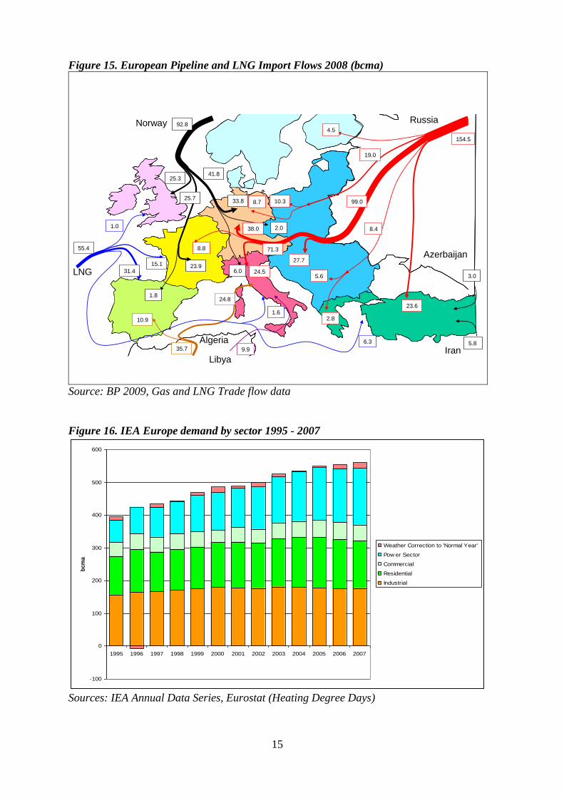
15
Figure 15. European Pipeline and LNG Import Flows 2008 (bcma)
154.5
99.0
19.0
4.5
5.6
8.4
2.8
23.6
27.7
10.38.7
38.0
71.38.8
24.5
92.8
1.8
41.825.3
2.0
6.023.9
33.8
35.7
10.9
24.8
5.8
3.0
Azerbaijan
9.9
55.4
1.0
31.4
15.1
1.6
6.3
Iran
Norway
Algeria
Libya
LNG
Russia
25.7
Source: BP 2009, Gas and LNG Trade flow data
Figure 16. IEA Europe demand by sector 1995 - 2007
-100
0
100
200
300
400
500
600
1995 1996 1997 1998 1999 2000 2001 2002 2003 2004 2005 2006 2007
bcm
a
Weather Correction to 'Normal Year'
Pow er Sector
Commercial
Residential
Industrial
Sources: IEA Annual Data Series, Eurostat (Heating Degree Days)

16
In the early 2000s a continuation of power sector gas demand growth led policy makers to
question where the additional supply might come from, given the likelihood that the
majority of incremental volumes would be imported gas. The ongoing disharmony
between Russia and Ukraine prompted concern as to the reliability of supply from this
quarter, despite Russia‟s excellent record as a reliable supplier since the 1970s. January
2006 saw Russia shutting off gas supplies to Ukraine with collateral damage of restricted
supply to some European countries, albeit brief. A more fundamental concern was the
growing realisation that in order to substantially increase exports to Europe, Russia would
need a substantial investment in key upstream projects such as the Yamal (Bovanenskoye)
and Shtokmanovskoye fields both to offset the ongoing decline from its giant Soviet-era
fields and to meet Russian domestic demand, which in the period 1999 to 2005 grew at an
annual average rate of 2%.13
The oft repeated mantra „Europe is surrounded by a sea of gas‟ seemed to offer scant
comfort in the context of little tangible progress being evident, (at the time), in securing
these supplies. The Nordstream project was the focus of attention through much of this
period (from West Siberia, via the Baltic Offshore to Germany and potentially the UK).
However, this project increasingly came to be recognised as a „Ukraine transit avoidance
route‟; rather than one offering significant net incremental gas supplies14
. Attention and
energy was focussed on the Nabucco or „4th
Corridor‟ project, spurred on by the success of
the Azerbaijan Shah Deniz project in successfully delivering gas to Turkey via a new
pipeline. The Nabucco project at the time of writing has political and downstream support
but still crucially lacks the committed upstream supply required to underpin such an
ambitious scheme. (For further discussion of these issues see Pirani 2009, pp. 404-406)
Figure 17. European Domestic Production 2000 - 2008
0
50
100
150
200
250
300
350
400
2000 2001 2002 2003 2004 2005 2006 2007 2008
bc
ma
Norway
Other
Romania
Denmark
Germany
Italy
Netherlands
UK
Source: IEA Monthly Data Series
13
BP 2009, Gas Consumption sheet. 14
It should be added however that the Shtokman field, whose likely start date is uncertain, may provide future
additional supplies via the Nordstream pipeline.

17
A key exacerbating factor was, with the exception of Norway, the ongoing decline in
European domestic production, especially in the UK, (Figure 17). Given the encyclopaedic
data and production forecasts available on North Sea UK Sector, coupled with a dearth of
new gas discoveries in the preceding years, it is astonishing, in retrospect, that the onset of
decline in the UK sector should have come as a surprise. The Department of Trade and
Industry and the UK Offshore Operators Association were, in the early 2000s, on a joint
aspirational mission to maintain UK oil and gas production „flat to 2010‟15
. This „Canute-
like‟ stance meant that when, in due course, it became evident that UK gas production had
commenced its decline, precious time had been lost. As a consequence, the delayed
implementation of new import projects was a key contributory cause of the tight supply
situation which faced the UK gas market during the period 2004 to 2006.
The period 2000 to 2005 also saw a sustained increase in the level of gas prices in Europe
(See Figure 18).
Figure 18. AGIP and Brent 2000 – 2005
0
1
2
3
4
5
6
7
8
9
10
Jan-00 Jan-01 Jan-02 Jan-03 Jan-04 Jan-05
$/m
mb
tu
0
10
20
30
40
50
60
70
Bre
nt
$/b
bl
AGIP Brent
Sources: Gas Matters, Platts
In the late 1990s the Average German Import Price (AGIP), (a blend of oil indexed long
term contract gas prices from Russia, Norway and the Netherlands), had remained in the $2
to $3/mmbtu range. A rise in the price of oil and oil products in 2000 took the AGIP price,
(linked to oil product prices with a 6 – 9 month lag), to $4/mmbtu briefly by the end of
15
UKOOA 2004

18
2000. After a lull in 2001 the oil price began its sustained rise, taking AGIP to $4/mmbtu
for 2003 and 2004 and then on up to around $7/mmbtu by the end of the following year.
The structure of the continental European natural gas market has been heavily influenced
by the discovery and commercialisation of the Groningen Field in Holland and pipeline
imports from Russia/Former Soviet Union. Gas from the Groningen field was priced, not
on its underlying cost of supply or on the basis of supply and demand but on the basis of
competitiveness with the final consumer‟s alternative non-gas fuels. This is often termed
the „market value principle‟ or alternatively the „netback market approach‟16
. The approach
was subsequently adopted for contracted pipeline and LNG imports to continental Europe.
In the UK cost-based pricing was the main principle used in the negotiation of contracts
between the state monopoly buyer British Gas and upstream producers in the pre-
liberalisation era (pre-1996)17
. This led to a wide range of contract prices depending on the
cost base and gas:liquids production ratio of fields specific to the contracts negotiated.
Contracts for European pipeline imports initiated from the 1970s to the present day are
typically 20 to 25 years in duration. The buyer has the right to nominate up to an annual
amount (the Annual Contract Quantity – or ACQ) but must take or in any case pay for an
annual quantity equal to the „Take or Pay‟ level (TOP), which is typically some 85% of the
ACQ on an annual basis. Additional flexibility is employed at the monthly or daily level
provided that in the course of a gas contract year an amount at least equal to the TOP is
paid for.
Pricing of long-term contracted gas imports is generally linked to the price of Gas Oil
and/or Fuel Oil, by a formula negotiated and defined in the contract:
Pn = Po +a*(av Fo(n-x ..n-1))+b*(av Go(n-x ... n-1))
The price in month n equals the initial contract price (Po) plus:
A constant a multiplied by the average of the last x-1 month‟s Fuel Oil
prices,
A constant b multiplied by the average of the last x-1 month‟s Gas Oil
prices
The values of the key variables are confidential to the parties to the contract, however they
have over time been inferred from border price data. These contracts also provide for
periodic price re-negotiation, or „price re-openers‟ if market conditions change
significantly. For this reason, in continental Europe there is a significant level of price
similarity in contract gas from different sources (Figure 19). This was not the case in the
UK, where contracts did not provide for price re-opener negotiations.
16
Stern 2007, pp 2-3 17
Stern 2007, p 4.

19
Figure 19. Oil Indexed Gas Prices in Europe 1997 - 2009
0
2
4
6
8
10
12
14
16
Jan-
97
Jan-
98
Jan-
99
Jan-
00
Jan-
01
Jan-
02
Jan-
03
Jan-
04
Jan-
05
Jan-
06
Jan-
07
Jan-
08
Jan-
09
$/m
mb
tu
AGIP
Troll
Russian Gas German Border
Dutch Gas German Border
Norway Gas German Border
Italian Average
Sources: Argus, Gas Matters
Prior to 1990 the UK market was dominated by British Gas – then the nationalised state
monopoly. Successive legislation served to progressively undermine this position,
critically that which allowed upstream producers to sell gas direct to the power sector and
large industrial users. This catalysed the monetisation of the „backlog‟ of undeveloped
offshore gas discoveries which then competed aggressively for customers in the power and
industrial sectors. BG‟s market share loss was such that it was unable to sell-on the take or
pay quantities under its field-specific long term contracts, and was increasingly priced out
of the market. BG also had to publish its industrial prices and hold them at those levels for
a defined period, allowing its competitors to undercut them with impunity.
Facing significant financial exposure BG was forced to re-negotiate many of its North Sea
purchase contracts and transform them to non-field specific long term supply contracts.
Although possibly some 25% of UK production is still sold under these surviving supply
contracts, their disparate pricing formulae have resulted in a significant degree of scatter
and as a result these do not influence the traded UK gas price.
The UK market became effectively liberalised in the mid 1990s with the NBP (National
Balancing Point) becoming a virtual hub18
.
18
For a full account of this see Wright 2006.
20
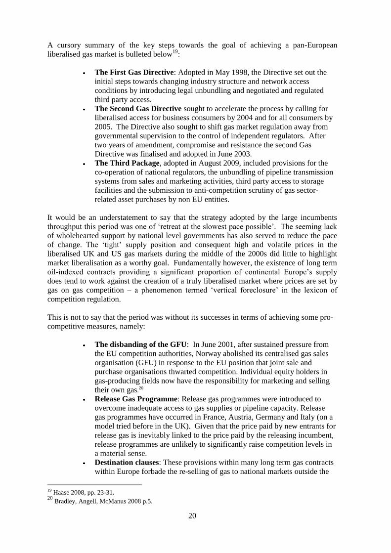
A cursory summary of the key steps towards the goal of achieving a pan-European
liberalised gas market is bulleted below19
:
The First Gas Directive: Adopted in May 1998, the Directive set out the
initial steps towards changing industry structure and network access
conditions by introducing legal unbundling and negotiated and regulated
third party access.
The Second Gas Directive sought to accelerate the process by calling for
liberalised access for business consumers by 2004 and for all consumers by
2005. The Directive also sought to shift gas market regulation away from
governmental supervision to the control of independent regulators. After
two years of amendment, compromise and resistance the second Gas
Directive was finalised and adopted in June 2003.
The Third Package, adopted in August 2009, included provisions for the
co-operation of national regulators, the unbundling of pipeline transmission
systems from sales and marketing activities, third party access to storage
facilities and the submission to anti-competition scrutiny of gas sector-
related asset purchases by non EU entities.
It would be an understatement to say that the strategy adopted by the large incumbents
throughput this period was one of „retreat at the slowest pace possible‟. The seeming lack
of wholehearted support by national level governments has also served to reduce the pace
of change. The „tight‟ supply position and consequent high and volatile prices in the
liberalised UK and US gas markets during the middle of the 2000s did little to highlight
market liberalisation as a worthy goal. Fundamentally however, the existence of long term
oil-indexed contracts providing a significant proportion of continental Europe‟s supply
does tend to work against the creation of a truly liberalised market where prices are set by
gas on gas competition – a phenomenon termed „vertical foreclosure‟ in the lexicon of
competition regulation.
This is not to say that the period was without its successes in terms of achieving some pro-
competitive measures, namely:
The disbanding of the GFU: In June 2001, after sustained pressure from
the EU competition authorities, Norway abolished its centralised gas sales
organisation (GFU) in response to the EU position that joint sale and
purchase organisations thwarted competition. Individual equity holders in
gas-producing fields now have the responsibility for marketing and selling
their own gas.20
Release Gas Programme: Release gas programmes were introduced to
overcome inadequate access to gas supplies or pipeline capacity. Release
gas programmes have occurred in France, Austria, Germany and Italy (on a
model tried before in the UK). Given that the price paid by new entrants for
release gas is inevitably linked to the price paid by the releasing incumbent,
release programmes are unlikely to significantly raise competition levels in
a material sense.
Destination clauses: These provisions within many long term gas contracts
within Europe forbade the re-selling of gas to national markets outside the
19
Haase 2008, pp. 23-31. 20
Bradley, Angell, McManus 2008 p.5.
21
original destination market. As a consequence of competition rules, such
provisions were removed from contracts, including those of Gazprom,
Sonatrach and LNG sellers.21
Despite the moves by the European Commission to liberalise the continental European gas
market it is still, in the author‟s opinion, in a state of „suspended animation‟: held back by
the interests of its gas market incumbents who have little incentive to change and whose
long term contractual arrangements with suppliers are difficult to reconcile with the
liberalised gas market model epitomised by the UK and North America. This „clash of
paradigms‟ is a key feature of a later section of this paper and is at the heart of the new
global dynamic in gas market arbitrage.
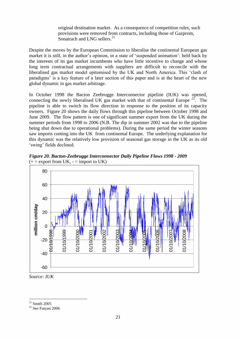
In October 1998 the Bacton Zeebrugge Interconnector pipeline (IUK) was opened,
connecting the newly liberalised UK gas market with that of continental Europe 22
. The
pipeline is able to switch its flow direction in response to the position of its capacity
owners. Figure 20 shows the daily flows through this pipeline between October 1998 and
June 2009. The flow pattern is one of significant summer export from the UK during the
summer periods from 1998 to 2006 (N.B. The dip in summer 2002 was due to the pipeline
being shut down due to operational problems). During the same period the winter seasons
saw imports coming into the UK from continental Europe. The underlying explanation for
this dynamic was the relatively low provision of seasonal gas storage in the UK as its old
„swing‟ fields declined.
Figure 20. Bacton-Zeebrugge Interconnector Daily Pipeline Flows 1998 - 2009
(+ = export from UK, - = import to UK)
-60
-40
-20
0
20
40
60
80
01/1
0/1
998
01/1
0/1
999
01/1
0/2
000
01/1
0/2
001
01/1
0/2
002
01/1
0/2
003
01/1
0/2
004
01/1
0/2
005
01/1
0/2
006
01/1
0/2
007
01/1
0/2
008
millio
n c
m/d
ay
Source: IUK
21
Smith 2005 22
See Futyan 2006

22
The summer export volumes peaked in 2003, with the decline in subsequent years driven
by the reduction in UK domestic production. Similarly the scale of winter imports can be
observed to increase through to the end of 2005. In October 2006 the Langeled pipeline
from Norway to the UK was completed, allowing additional imports to the UK. A year
later the Ormen Lange field commenced production adding further to UK gas imports.
The additional supplies from Norway appear to have stabilized the trend of reducing
summer exports and growing winter imports through the Bacton-Zeebrugge Interconnector
and in addition appear to have increased the short term volatility of daily flowrates.
Following the opening of the IUK, UK and continental oil indexed gas prices were
reasonably well correlated through to the spring of 2001 (Figure 21). The years 2001 to
2003 were characterised by reasonably close price correlation during the winter months but
with NBP de-linking and falling during the summer. 2001 to 2003 was a period of peak
summer export of gas from the UK. From 2004 onwards, evidence of increasing supply
tightness is apparent.
Figure 21. UK NBP Spot Price and German Average Import Gas Price (AGIP) January
1997 – November 2009
0
2
4
6
8
10
12
14
16
Jan-9
7
Jan-9
8
Jan-9
9
Jan-0
0
Jan-0
1
Jan-0
2
Jan-0
3
Jan-0
4
Jan-0
5
Jan-0
6
Jan-0
7
Jan-0
8
Jan-0
9
Gas P
ric
e $
/mm
btu
NBP
AGIPInterconnector Opens
Convergence periods
Sources: Argus, Gas Matters
In 2004 and early 2005 there is close correlation between the UK and continental prices but
in 4Q05 NBP de-links and soars to unprecedented price levels. An early spell of cold
weather increased UK demand in November 2005. It was soon apparent, however, that
owners of gas in storage in continental Europe were not prepared to send as much gas to
the UK as price signals called for due to their concerns over having sufficient storage
inventory to meet the demands of their own domestic customers through the rest of the
23
winter. These concerns were driven by public service obligations which are widespread in
continental Europe. Throughout that winter Asian LNG markets were bidding in excess of
$15/mmbtu for spot LNG cargoes as Indonesian underperformance reduced availability of
contracted LNG in those markets. The tight UK supply situation was further exacerbated
by operational problems at the UK‟s largest seasonal gas storage facility (the depleted
Rough gas field) which reduced supply in 1 and 2Q 2006.
In October 2006 famine turned to feast when the Langeled pipeline came onstream and low
UK prices continued until late 2007 when NBP once again converged with AGIP up until
3Q08. This later convergence was in all probability due to the tightening of supply due to
the ongoing decline of the UK‟s domestic gas production.
Let us now examine the mechanics of the North West Europe hubs which are the physical
interface between „spot gas‟ and oil indexed pipeline gas.
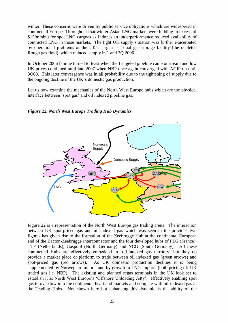
Figure 22. North West Europe Trading Hub Dynamics
NBP
PEGNCG
TTF
Zee
Norwegian
Supply
Domestic Supply
LNG
GASPOOL
Figure 22 is a representation of the North West Europe gas trading arena. The interaction
between UK spot-priced gas and oil-indexed gas which was seen in the previous two
figures has given rise to the formation of the Zeebrugge Hub at the continental European
end of the Bacton-Zeebrugge Interconnector and the four developed hubs of PEG (France),
TTF (Netherlands), Gaspool (North Germany) and NCG (South Germany). All these
continental Hubs are effectively embedded in „oil-indexed gas territory‟ but they do
provide a market place or platform to trade between oil indexed gas (green arrows) and
spot-priced gas (red arrows). As UK domestic production declines it is being
supplemented by Norwegian imports and by growth in LNG imports (both pricing off UK
traded gas i.e. NBP). The existing and planned regas terminals in the UK look set to
establish it as North West Europe‟s „Offshore Unloading Jetty‟; effectively enabling spot
gas to overflow into the continental heartland markets and compete with oil-indexed gas at
the Trading Hubs. Not shown here but enhancing this dynamic is the ability of the

24
Zeebrugge LNG regas terminal and by 2012, once commissioned, the GATE LNG terminal
in the Netherlands, to receive spot cargoes.
So how does the arbitrage dynamic operate at the trading hubs ?
Figure 23. Dynamics of North West Europe Trading Hubs
Trading HubTake-or-Pay Volume
Spot Gas FlowOil Indexed Contract
Gas Flow
Storage Facility
Volume up to Annual
Contract Quantity
A hub is schematically represented in Figure 23. Let us consider two cases:
The spot gas price is lower than the oil-indexed gas price: In this situation,
midstream gas players at the hubs will buy up more spot gas and buy less oil indexed
gas. This will have the effect of pulling more gas out of the UK and causing the NBP
price to rise. As the demand for oil-indexed gas falls, buyers with long term contracts
will reduce their nominations – effectively taking gas „out of the system‟ as it is left in
the gas field upstream. This process repeats itself until either:
NBP has risen to equal the continental oil-indexed price; or,
The supply of oil-indexed gas has been reduced to its take-or-pay level and
the process of arbitrage can proceed no further.
The spot gas price is higher than the oil-indexed gas price: In this situation,
midstream gas players at the hubs will buy less spot gas and buy more oil-indexed gas.
This will have the effect of pulling less gas out of the UK (and could send gas which
was oil-indexed into the UK), causing the price to fall. As the demand for oil-indexed
gas rises, buyers under these long term contracts will increase their nominations-
effectively bringing extra gas „into the system‟ through higher upstream production.
This process repeats itself until either:

25
NBP has fallen to equal the continental oil-indexed price; or,
The supply of oil-indexed gas has been increased to its annual contract
quantity (ACQ) level and the process of arbitrage can proceed no further.
Three overlays on this central concept need to be noted:
The arbitrage can be „time parked‟23
by the use of gas storage facilities.
Historically, storage usage in continental Europe has been driven by a
conservative „utility‟ mindset24
, however the author believes that much of
the current and future salt cavern storage development in North West
Europe is driven by the prospect of spot vs. oil-indexed price arbitrage.
It is likely that arbitrage is restricted by pipeline infrastructure bottlenecks,
(„connectivity‟), as well as by contractual flexibility limits.
The reference to take-or-pay and annual contract quantity levels as
limitations at the monthly level is simplistic. In practice there is greater
short term flexibility as long as these levels are adhered to on a cumulative
basis by the end of the „gas contract year‟ which runs from October 1st to
September 30th
.
This framework explains the recurrence of price convergence in Figure 21.
Evidence of the scale of linkage between North West Europe‟s gas trading hubs is difficult
to establish in terms of transportation capacities, however the evidence for price linkage is
compelling, as is shown in Figure 24, which is only possible with physical connectivity
between these hubs and gas flows through IUK and BBL.
Figure 24. North West Europe Hub Prices January2008 – March 2009
Source: ICE (Intercontinental Exchange)
23
„Time Parked‟ – shorthand for the action of trading entities injecting into storage gas purchased at low
prices with the intention of withdrawing and selling this during periods when the hub price is higher. 24
„Utility Mindset‟ – with reference to storage this means only using storage to meet demand peaks and to
provide supply security.

26
Asia LNG Market Structure and Developments
As depicted in Figure 25, Asia (and in particular Japan) began to dominate the global LNG
picture by the late 1970s and continues to be the largest single importing regional market.
Japan, South Korea and Taiwan, lacking significant domestic production, rely on LNG for
their natural gas requirements. The market context and supply security mindset so
engendered has been largely responsible for the somewhat „traditional‟ supply contracting
custom and practice which has characterised Asian LNG.
Figure 25. Global LNG Imports by Country 1964 - 2008
0
50
100
150
200
250
1964
1967
1970
1973
1976
1979
1982
1985
1988
1991
1994
1997
2000
2003
2006
bc
ma
Puerto Rico
Dominican Republic
Mexico
US
Tunisia
UK
Turkey
Spain
Portugal
Italy
Greece
France
Belgium
India
China
Taiw an
South Korea
Japan
N America
Europe
Asia
Sources: Cedigaz 2004, BP 2009 (Gas Trade Movements LNG)
Asia‟s gas consumption (Figure 26) grew at 6.5% per annum from 1995 to 2000 and
continued at 6.4% per annum from 2000 to 2008.
What is interesting is the variation in demand growth rates over the period 1995 – 2008
between countries with Australia and Japan in the 1 to 4 % p.a. range on the one hand and
South Korea and China at 11.0% and 12.6% respectively (Figure 27).

27
Figure 26. Asia Annual Natural Gas Consumption 1995 - 2008
0
50
100
150
200
250
300
350
400
450
500
1995 1996 1997 1998 1999 2000 2001 2002 2003 2004 2005 2006 2007 2008
bc
ma
Other Asia Pacific
Thailand
Taiwan
South Korea
Singapore
Philippines
Pakistan
New Zealand
Malaysia
Japan
Indonesia
India
China
Bangladesh
Australia
Source: BP 2009, (Natural Gas Consumption sheet)
Figure 27. Asia Compound Annual Average Demand Growth 1995 - 2008
Compound Annual
Average Growth in
Demand %
Australia 1.4%
Bangladesh 6.8%
China 12.6%
India 6.3%
Indonesia 2.3%
Japan 3.8%
Malaysia 6.4%
Pakistan 5.7%
South Korea 11.0%
Taiwan 8.6%
Thailand 9.6% Source: BP 2009 (Natural Gas Consumption sheet)
The Asian natural gas supply-demand dynamics are better grasped by grouping the
countries in terms of import dependence during this period:
Producers with a surplus for export: Australia, Indonesia, Malaysia. It should be noted
that in the case of Indonesia in particular, the high rate of growth of domestic consumption
has started to limit the scope for LNG exports, and this trend is increasing.

28
Producers meeting indigenous demand: Bangladesh, New Zealand, Pakistan,
Philippines, Thailand.
Net Importers: China, India, Japan, South Korea, Taiwan
However before we look at the natural gas trade flow dynamics it is important to appreciate
how small a share of primary energy natural gas currently represents in this region. For
instance, in China natural gas in 2005 constituted only 3% of fossil fuel consumption
(Figure 28), and in 2006 natural gas contributed only 9% of India‟s primary energy
consumption (Figure 29).
Figure 28. China Fossil Fuel Consumption 1995 - 2005
0
500
1000
1500
2000
2500
1990 1991 1992 1993 1994 1995 1996 1997 1998 1999 2000 2001 2002 2003 2004 2005
Mil
lio
ns
To
nn
es
Co
al
Eq
uiv
ale
nt
Pe
r Y
ea
r
Natural Gas
Oil
Coal
Source: OIES Asia 2008, Table 2.1, p. 9.
Figure 29. India Primary Energy Consumption 2006
Coal
56%
Gas
9%
Oil
28%
Hydro
6%
Nuclear
1%
Source: OIES Asia 2008, Table 2.1, p. 9.

29
Data for Asia is unfortunately not particularly comprehensive and therefore a region-wide
natural gas consumption sectoral analysis is not presented here.
Figure 30 shows the growth in LNG imports in Japan, Korea and Taiwan, (where LNG is
the only significant source of natural gas) and India and China, where LNG supplements
indigenous production in meeting natural gas demand.
Figure 30. Asia Market LNG Imports 1995 - 2008
0
20
40
60
80
100
120
140
160
180
1995 1996 1997 1998 1999 2000 2001 2002 2003 2004 2005 2006 2007 2008
bcm
a
China
India
Taiwan
South Korea
Japan
Source: BP 2009, (LNG Gas Trade Sheet)
The jump in Japanese LNG imports in 2007 was in part caused by the prolonged shutdown
of the 6.6MW Kashiwazaki Kariwa nuclear power plant in July 2007 following a severe
earthquake. Two units of the plant were re-started in late 2009 and early 2010.
The traditional Asian LNG project featured a carefully structured system of risk sharing
amongst the participants, central to which was the long term LNG (Purchase and Sales)
contract, typically of 20 years or longer duration. As with long term pipeline contracts the
risk sharing logic of the contract is often expressed by the phrase „the buyer takes the
volume risk and the seller takes the price risk‟. Most contracts featured „Take-or-Pay‟
provisions to assure buyer off-take at a minimum level, to guarantee cash flow to the seller,
and a price indexation clause to expose the seller to energy price fluctuations.
In the typical setting nearly all buyers were government monopoly or franchised utility
companies from OECD countries and sellers typically major or national oil and gas
companies. The level of credit-worthiness of participants facilitated favourable financing
terms25
. In its original form the LNG contract envisaged a system in which particular
trades are self-contained, involving a specified liquefaction facility as the source of LNG
and dedicated tankers to transport it to its specific destination.
25
„Jensen 2004, p 15.
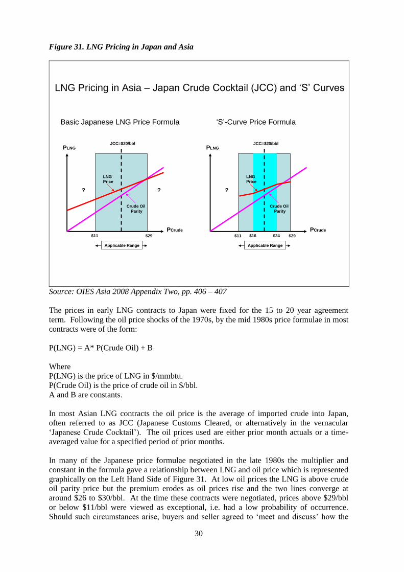
30
Figure 31. LNG Pricing in Japan and Asia
$11 $29
JCC=$20/bbl
PCrude
PLNG
Applicable Range
? ?
LNG
Price
Crude Oil
Parity
$11 $29
JCC=$20/bbl
PCrude
PLNG
Applicable Range
?
LNG
Price
Crude Oil
Parity
$16 $24
LNG Pricing in Asia – Japan Crude Cocktail (JCC) and ‘S’ Curves
Basic Japanese LNG Price Formula ‘S’-Curve Price Formula
Source: OIES Asia 2008 Appendix Two, pp. 406 – 407
The prices in early LNG contracts to Japan were fixed for the 15 to 20 year agreement
term. Following the oil price shocks of the 1970s, by the mid 1980s price formulae in most
contracts were of the form:
P(LNG) = A* P(Crude Oil) + B
Where
P(LNG) is the price of LNG in $/mmbtu.
P(Crude Oil) is the price of crude oil in $/bbl.
A and B are constants.
In most Asian LNG contracts the oil price is the average of imported crude into Japan,
often referred to as JCC (Japanese Customs Cleared, or alternatively in the vernacular
„Japanese Crude Cocktail‟). The oil prices used are either prior month actuals or a time-
averaged value for a specified period of prior months.
In many of the Japanese price formulae negotiated in the late 1980s the multiplier and
constant in the formula gave a relationship between LNG and oil price which is represented
graphically on the Left Hand Side of Figure 31. At low oil prices the LNG is above crude
oil parity price but the premium erodes as oil prices rise and the two lines converge at
around $26 to $30/bbl. At the time these contracts were negotiated, prices above $29/bbl
or below $11/bbl were viewed as exceptional, i.e. had a low probability of occurrence.
Should such circumstances arise, buyers and seller agreed to „meet and discuss‟ how the

31
price of LNG would be derived. South Korea and Taiwan adopted a similar approach in the
late 1980s and early 1990s, but the straight line relationship was not restricted to an
applicable range.
In the early 1990s when many Japanese contracts came up for renegotiation, the impact on
LNG prices of „extreme‟ oil prices was mitigated by the introduction of the „S‟- Curve
relationship, shown on the Right Hand Side of Figure 31. Further modifications were made
to this approach in the 2000s to further soften the impact of high oil prices.26
For a regional market which espouses the importance of „stability‟ and „long term
relationships‟, the data available on LNG import prices in these markets paints a
surprisingly diverse picture (Figure 32).
Figure 32. Asian LNG Prices – March 2004 – February 2009
0
5
10
15
20
25
Mar
-04
Jun-
04
Sep
-04
Dec
-04
Mar
-05
Jun-
05
Sep
-05
Dec
-05
Mar
-06
Jun-
06
Sep
-06
Dec
-06
Mar
-07
Jun-
07
Sep
-07
Dec
-07
Mar
-08
Jun-
08
Sep
-08
Dec
-08
$/m
mbtu
Abu Dhabi - Japan
Algeria - Japan
Australia - Japan
Brunei - Japan
Eq Guinea - Japan
Indonesia - Japan
Malaysia - Japan
Nigeria - Japan
Oman - Japan
Qatar - Japan
US - Japan
Indonesia - Taiwan
Malaysia - Taiwan
South Korea - Average
Source: Argus
Whilst in March 2004 the import prices of LNG in the Asian importing markets were
reasonably tightly bounded, by 2008 the combination of different oil price escalators and
the plethora of S curves and differing indices and parameters have resulted in a wide
divergence of price for what is essentially the same commodity. Note that each of these
data series represents a „bundle‟ of individual contracts; the range at the individual contract
level will be wider.
The early 2000s became a challenging time for the prevailing contracting philosophy of the
Asian LNG market due to:
The under-performance of Indonesia as an LNG exporter as shown in Figure
33.
The rapid growth in natural gas demand as shown in Figure 26.
26
OIES Asia 2008, Appendix Two, pp 405 – 408.

32
The slippage of LNG supply projects generally, as shown later in Figure 37.
Recurring Japanese nuclear generation problems requiring increasing usage
of LNG-fired units.
A decision by Korea to restrict LNG imports to those under contracts by
power generation companies and to preclude city gas companies from
signing new LNG import contracts.27
Figure 33. Indonesia LNG Exports
0
5
10
15
20
25
30
35
40
45
1995 1996 1997 1998 1999 2000 2001 2002 2003 2004 2005 2006 2007 2008
bcm
a
Source: BP 2009, Cedigaz 2004
Due to the lack of suitable geological structures and possibly also as a consequence of rapid
gas market growth, Asia is poorly provided with gas storage other than in the form of LNG
regas storage tanks. Due to the almost total reliance on LNG as their natural gas supply,
Japan, Korea and Taiwan have tended to keep LNG storage tanks relatively full and to
meet winter demand through additional winter LNG imports.
The factors listed above drove Asian LNG importers to enter the spot market for LNG in
the winters of 2005/2006, 2006/2007 and 2007/2008 to a significant extent, pulling spot
cargoes out of the Atlantic Basin. The prices paid varied widely with no obvious pattern.
It is known that Japan and Korea burn residual fuel oil, crude and distillate in their power
generation sectors and some, if limited, correlation to these substitute fuels can be seen in
Figure 34.
For the winter of 2005/2006 the high spot LNG prices exceeded gas oil prices. There is no
rational explanation for this other than that this was a period of general supply tightness
with Hurricane Katrina having hit much US gas production and the UK market also in a
tight position. In winter 2006/2007 there appeared to be a more rational correlation
between high LNG spot prices and gas oil price. In winter 2007/2008 high spot prices
appear to be correlated to residual fuel oil (LSFO). Suffice to say that the general market
awareness of the extent of Asia spot LNG purchase during this period impacted the markets
of Europe and to some degree indirectly North America in the first half of 2008. (For a
wider appreciation of the implications of LNG pricing relative to alternative fuels in Asian
markets please see Miyamoto & Ishiguro 2006).
27 OIES Asia 2008, pp 174 - 211

33
Figure 34. Range of Asia LNG Spot Prices 2004 – 2008
0
5
10
15
20
25
Ja
n-0
4
Ma
r-0
4
Ma
y-0
4
Ju
l-0
4
Se
p-0
4
No
v-0
4
Ja
n-0
5
Ma
r-0
5
Ma
y-0
5
Ju
l-0
5
Se
p-0
5
No
v-0
5
Ja
n-0
6
Ma
r-0
6
Ma
y-0
6
Ju
l-0
6
Se
p-0
6
No
v-0
6
Ja
n-0
7
Ma
r-0
7
Ma
y-0
7
Ju
l-0
7
Se
p-0
7
No
v-0
7
Ja
n-0
8
$/m
mb
tu
Low
Average
High
LSFO
Brent
Gas Oil
Source: FACTS 2008
The Renaissance of LNG
As we have discussed in previous sections the concern of importing markets from 2000 to
2005 was how anticipated future gas demand growth would be met by supply given:
The ongoing decline in indigenous production in Europe and North America.
The uncertainty on timing and incremental volumes available from pipeline import
projects for Europe particularly and
The unexpected decline in LNG supply from Indonesia.
The prevailing industry perception of a „tight‟ market for the foreseeable future provided
fertile ground for the progression of numerous LNG supply projects. The surge in LNG
FID‟s (Final Investment Decisions) is shown in Figure 35. There was an unprecedented
activity peak in the period 2002 - 2005 which subsequently strained the capacity of the few
specialist liquefaction engineering contractors able to construct this number of liquefaction
plant simultaneously. Coming on top of the rise in commodity prices, this resulted in a
reversal in the downward trend in unit liquefaction capital costs (Figure 36), thus
challenging project economics and available financing and constraining the pace of new
commitments later in the period. These factors conspired to cause an ongoing slippage in
the aggregate (industry) ten year forecast of future LNG supply capacity, as is shown in
Figure 37.
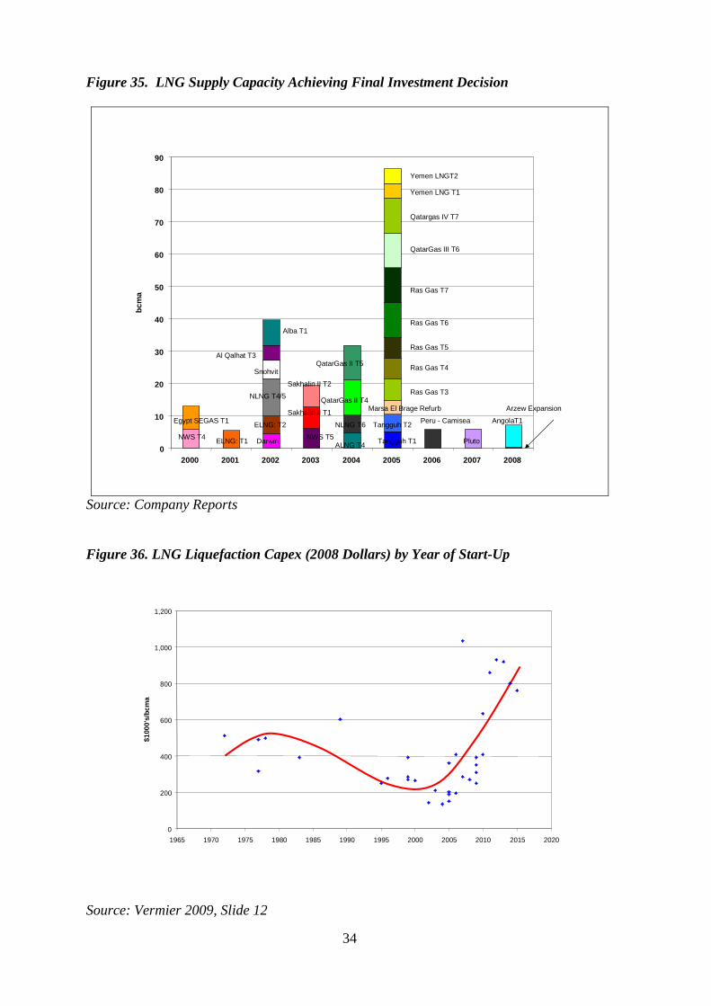
34
Figure 35. LNG Supply Capacity Achieving Final Investment Decision
0
10
20
30
40
50
60
70
80
90
2000 2001 2002 2003 2004 2005 2006 2007 2008
bc
ma
Yemen LNGT2
Yemen LNG T1
ALNG T4
Sakhalin II T2
Sakhalin II T1
Qatargas IV T7
QatarGas III T6
Ras Gas T7
Ras Gas T6
Ras Gas T5
QatarGas II T5
QatarGas II T4
Ras Gas T4
Ras Gas T3
Peru - Camisea
Al Qalhat T3
Snohvit
NLNG T6
NLNG T4/5
Marsa El Brage Refurb
Tangguh T2
Tangguh T1
Alba T1
Egypt SEGAS T1ELNG: T2
ELNG: T1 PlutoNWS T5
DarwinNWS T4
AngolaT1
Arzew Expansion
Source: Company Reports
Figure 36. LNG Liquefaction Capex (2008 Dollars) by Year of Start-Up
0
200
400
600
800
1,000
1,200
1965 1970 1975 1980 1985 1990 1995 2000 2005 2010 2015 2020
$1
00
0's
/bc
ma
Source: Vermier 2009, Slide 12
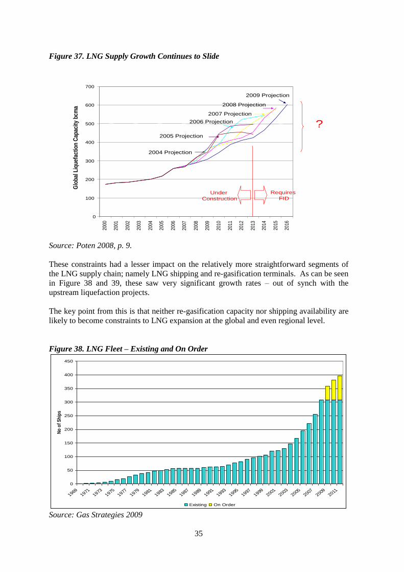
35
Figure 37. LNG Supply Growth Continues to Slide
2009 Projection
2008 Projection
2007 Projection
2006 Projection
2005 Projection
2004 Projection
Under
Construction
Requires
FID
?
0
100
200
300
400
500
600
700
2000
2001
2002
2003
2004
2005
2006
2007
2008
2009
2010
2011
2012
2013
2014
2015
2016
Glo
bal
Liq
uef
acti
on
Cap
acit
y b
cma
Source: Poten 2008, p. 9.
These constraints had a lesser impact on the relatively more straightforward segments of
the LNG supply chain; namely LNG shipping and re-gasification terminals. As can be seen
in Figure 38 and 39, these saw very significant growth rates – out of synch with the
upstream liquefaction projects.
The key point from this is that neither re-gasification capacity nor shipping availability are
likely to become constraints to LNG expansion at the global and even regional level.
Figure 38. LNG Fleet – Existing and On Order
0
50
100
150
200
250
300
350
400
450
19691971
19731975
19771979
19811983
19851987
19891991
19931995
19971999
20012003
20052007
20092011
No
of
Sh
ips
Existing On Order
Source: Gas Strategies 2009

36
Figure 39. Global Regas Capacity 2000 – 2010 by Region
Asia
0
50
100
150
200
250
300
350
400
2000 2001 2002 2003 2004 2005 2006 2007 2008 2009 2010
bcm
a
Existing In Development
Europe
0
50
100
150
200
250
2000 2001 2002 2003 2004 2005 2006 2007 2008 2009 2010
bcm
a
US, Canada & Mexico
0
50
100
150
200
2000 2001 2002 2003 2004 2005 2006 2007 2008 2009 2010
bcm
a
Central & South America
0
50
100
150
2000 2001 2002 2003 2004 2005 2006 2007 2008 2009 2010
bc
ma
Source: WoodMac 2008a

37
The Mechanics of LNG Arbitrage and Activity to Date
Clearly the evidence of spot LNG purchases by Asian buyers since 2005 is part of a wider
move to „loosen up‟ the rather rigid business model of the traditional LNG business in
response to the irresistible motivation of short term self interest. Indeed given LNG‟s
uniquely mobile format, in the context of inherently disparate regional market pricing
structures, it was almost inevitable that sooner or later the „trading mindset‟ would gain
ground over the „long term relationships‟ paradigm.
The framework in which this trend can be analysed and quantified is the core of this paper
and the substance of Chapter 2. The next part of this section describes the mechanics of
LNG arbitrage.
Figure 40. Short Term Trading in LNG 1992 - 2008
0
50
100
150
200
250
1992
1993
1994
1995
1996
1997
1998
1999
2000
2001
2002
2003
2004
2005
2006
2007
2008
bcm
a
Short Term –
Including
Contracts of
Three Years or
Less
Long Term
Contract
2.5%
7.5%
11.6%
19.8% 17.8%
Source: Jensen 2009, Slide 23
By way of an overview, Figure 40 shows the growth of LNG sales classed as „short term‟
i.e. either spot sales or contracts of less than three years in duration. The majority of these
trades offer the potential for additional profit for the seller realised by diverting an LNG
cargo from the original destination market to an alternative, higher priced opportunistic
sale. This can be effected only where the original buyer (under the prevailing contract)
consents to such a trade inevitably induced by a share of the resulting profit margin.

38
Polina Zhuravleva28
describes four models of LNG arbitrage and three examples of short
term sales which fall short of a strict definition of arbitrage. An overview of her taxonomy
is contained in Appendix 1.
Flexible mechanisms have evolved to exploit short term price differentials for a limited
number of contracted LNG volumes. By 2012, significant volumes of LNG from new
supply projects will become available for which market destination has been deliberately
kept flexible.
Figure 41. Regional LNG Contract Commitments – 2008 Showing Uncommitted or Self
Contracted Volumes
0 10 20 30 40 50 60 70 80
Pacific Basin
Middle East
Atlantic Basin
bcma
Committed North America
Committed Europe
Committed Asia
Self Contracted
Uncommitted
These Volumes are Destination Flexible
Source: Jensen 2009, Slide 26
The segmentation of global LNG supply shown in Figure 41 is explained as follows.
The „committed‟ tranches are those under traditional long term contracts,
however, as we have seen above, if buyer and seller are amenable, it is
possible for some of these volumes to be diverted to exploit price
opportunities in markets other than that which was the originally intended
destination.
The „Self Contracted‟ tranche represents a relatively new phenomenon,
primarily represented by BG with Equatorial Guinea and ExxonMobil/Qatar
Petroleum with their Qatar LNG Projects. Instead of the traditional oil-
indexed take-or-pay long term contracts with in-country incumbents, this
form of contract involves the International Oil & Gas Company effectively
28
Zhuravleva 2009.

39
using its balance sheet as security and contracting to take the LNG volume
and place it in the market offering the best netback at the time. These self-
contracted segments represent significant volumes and are inherently price-
seeking flexible volumes mainly, but not exclusively, intended for Atlantic
Basin markets.
„Uncommitted Volumes‟ to date have been largely those cargoes which
have been produced:
in excess of envisaged early liquefaction train performance, before
contracts have fully „kicked in‟ at ACQ,
where the buyer has chosen to exercise downward flexibility on
contract volumes towards minimum take or pay levels and where the
seller wishes to produce at full capacity and sell the balance to
uncontracted buyers in an opportunistic manner.
The reality of the significant increase in short term opportunistic LNG trading is shown in
Figure 42 which shows the actual supply patterns of Algeria, Egypt, Qatar, Nigeria, Oman
and Trinidad from 2000 to 2008. At the beginning of the period LNG deliveries were
broadly in line with contractual provisions but since the mid 2000s we can see the
fragmentation of LNG deliveries which has been facilitated by the mechanisms described
above and incentivised by the regional price differentials created by different regional
market pricing structures. The areas circled in Figure 42 highlight the opportunistic sales
in the second half of the period.

40
Figure 42. Supply Patterns of Six LNG Producers 2000 - 2008
Oman Supply to Markets
0
2
4
6
8
10
12
14
2000 2001 2002 2003 2004 2005 2006 2007 2008
bc
ma
Argentina
Taiwan
India
China
UK
Turkey
Portugal
Italy
Greece
France
Belgium
Canada
Dominican Republic
Puerto Rico
Mexico
US
Spain
Japan
South Korea
Trinidad Supply to Markets
0
5
10
15
20
25
2000 2001 2002 2003 2004 2005 2006 2007 2008
bc
ma
Argentina
Japan
Taiwan
India
China
UK
Turkey
Portugal
Italy
Greece
France
Belgium
Canada
Dominican Republic
South Korea
Mexico
Puerto Rico
Spain
US
Nigeria Supply to Markets
0
5
10
15
20
25
2000 2001 2002 2003 2004 2005 2006 2007 2008
bc
ma
Argentina
South Korea
India
China
UK
Greece
Belgium
Canada
Japan
Dominican Republic
Puerto Rico
Mexico
Taiwan
US
Turkey
Portugal
Italy
France
Spain
Qatar Supply to Markets
0
5
10
15
20
25
30
35
40
45
2000 2001 2002 2003 2004 2005 2006 2007 2008
bc
ma
Argentina
Taiwan
China
UK
Turkey
Portugal
Italy
Greece
France
Canada
Dominican Republic
Puerto Rico
Mexico
US
Belgium
India
Japan
South Korea
Spain
Algeria Supply to Markets
0
5
10
15
20
25
30
2000 2001 2002 2003 2004 2005 2006 2007 2008
bc
ma
Argentina
Japan
Taiwan
South Korea
India
China
UK
Portugal
Greece
Belgium
Canada
Dominican Republic
Puerto Rico
Mexico
US
Italy
Turkey
Spain
France
Egypt Supply to Markets
0
2
4
6
8
10
12
14
16
2000 2001 2002 2003 2004 2005 2006 2007 2008
bc
ma
Argentina
Taiwan
India
China
UK
Turkey
Portugal
Italy
Greece
Belgium
Canada
Dominican Republic
Puerto Rico
Japan
South Korea
Mexico
US
France
Spain
Sources: BP 2009, Waterborne LNG
41
Market Developments in 2008 and 2009 - The Perfect Storm
To conclude this descriptive, context-setting chapter we summarise the main market
dynamics we have observed since 2000:
As we left the 1990s with the expectation of abundant, low cost natural gas a number of
developing trends heightened concern over supply sufficiency:
In North America gas production began to decline despite the rising rig
count in the period 2001 – 2005. Prices became volatile with extreme high
price excursions in response to weather and hurricane events.
In Europe, concerns mounted over the ability of future imported gas
supplies to keep pace with anticipated demand growth, especially in the
power generation sector. Long term contract prices rose significantly as oil
products prices began their sustained climb. UK prices became volatile with
weather/event driven high price excursions as domestic supplies declined.
In Asia the unforeseen decline in Indonesian LNG output and slippage in
LNG projects led to Asian importers „outbidding‟ Atlantic Basin buyers for
spot cargoes; this was perhaps exacerbated by the prospect of India and
China on the horizon as new LNG importers.
The „supply response‟ to these developments was two-fold:
A wave of new LNG projects was sanctioned with FIDs peaking in 2005.
However this intensity of activity strained contracting sector capacity,
resulting in project slippage and liquefaction unit cost inflation.
In parallel the decline in North American domestic production was reversed
due to the successful development of technology and approaches to exploit
„unconventional gas‟ namely shale gas and coal bed methane.
In parallel, the LNG world became more flexible in response to the arbitrage opportunities
available during the 2005 – 2008 period and also by virtue of new projects with market
destinations kept deliberately flexible.
The unexpected increase in North American production has threatened to oversupply the
domestic market and as a consequence US prices have softened in response. However
some of the new LNG supply about to come onstream was at least notionally tagged to the
North American market. Traded markets were likely to soften as a consequence even
without the 2009 slump in gas demand caused by the economic recession.
Recession-driven demand reductions for natural gas have been apparent since 4Q 2008 and
are particularly evident in the Asian markets of Japan, Korea and Taiwan and generally in
Europe.
The high production levels in North America combined with reduced demand levels in
many LNG importing markets, coupled with the imminent significant growth in LNG
supply will result in LNG-facilitated market interaction on a scale hitherto unknown.
The likely trends and discontinuities thus generated are examined quantitatively in Chapter
Three. Chapter Two develops the analytical framework to facilitate this.

42
2. The Framework for Future Market Interaction through LNG and
Pipeline Arbitrage
Introduction
This section describes a modelling framework which is able, subject to certain constraints
and simplifications, to explore how the three main regional gas markets interact, especially
as they become increasingly linked by LNG trade-flows.
Most modelling frameworks in the sphere of natural gas tend to be „cost of supply- based‟
despatch models with, at some stage, linear programming having a key role in defining the
„optimal‟ solution. The attraction in the use of Linear Programming is that it produces a
unique solution for systems which have multiple possibilities but for which iterative
analysis arrives at the „objective function‟ of, typically, a „lowest cost of supply‟ solution.
Applying such an approach to the real world of natural gas certainly has its attractions,
however it does tend to presume that the system does or „should‟ conform to a „perfect
market‟ in its behaviour. Rightly or wrongly the real world of natural gas only approaches
this paradigm in the liberalised markets of North America and the UK. Constraints can be
added to models such as:
for oil-indexed contract supply, the „cost of supply‟ can be substituted by the
oil product indexed price, driven off a view of future oil prices.
„must flow‟ rules for contract take-or-pay volumes.
Such models rapidly become highly complex to set up and to diagnose the rationale behind
a supposed „solution‟. If a model scope is constrained to focus on a specific regional
market it becomes flawed by the inability to address the changes in LNG supply between
regions which might come about as a consequence of price differentials. On the other
hand, if such a model does attempt to cover all major LNG consuming regions, it quickly
becomes hostage to the need to forecast the overwhelmingly important (but highly elusive)
nature of the future North American supply cost curve.
Having had mixed experience with such approaches in the past, the author derived a more
direct and transparent framework with the following conceptual elements:
A monthly global balance encompassing all natural gas supply and demand
of which LNG is one component.
Regions included in this balance are:
Europe (including Norway and Turkey), Asian LNG importers, US,
Canada and Mexico and new LNG „niche markets‟ outside the above
regions.
All global LNG supply.
Supply and demand are projected at a national market level but dynamics
are analysed at a regional level due to „degrees of freedom‟ constraints.
Instead of a Linear Programming approach, the analysis is „behavioural
rules‟ based and the main focus is the arbitrage – driven dynamic between
oil-indexed European pipeline gas and LNG which can be diverted between
Europe and North America.

43
This chapter describes the analytical framework so created and the quantitative analysis it
produces.
The Global LNG Analysis Conceptual Framework
From our previously discussed observations of the interaction between the liberalised UK
market and oil-indexed Europe since the opening of the Bacton-Zeebrugge Interconnector,
and the observed behaviours of the Asian and North American markets with regard to
LNG, we derive the following behavioural „Rules‟ for the regions:
Asia: For Japan, Korea and Taiwan, LNG represents the only significant supply of natural
gas. Security of supply is a fundamental concern for these markets. These markets have
entered into binding long-term contracts for LNG supply, however since 2005, due to the
slippage of new LNG supply projects and the underperformance of Indonesia as an LNG
supplier, they have resorted to purchasing spot LNG at prices equating, at times, to crude
and even distillate equivalent levels. These markets, for reasons of geology, lack
underground gas storage. They tend to keep their re-gas storage tanks at high inventory
levels – again for supply security reasons, rather than profiling inventory through the year
so as to take advantage of lower summer spot LNG prices. In short we assume that these
markets take „first call‟ on global LNG supply according to their forecast demand, paying
whatever price is required to secure spot supply over and above contracted supply if
necessary. India and China differ in that they also have indigenous natural gas supply.
This said however, prior to 2011 demand is limited by re-gas terminal capacity and
forecasts of LNG supply are bounded by these infrastructure constraints.
North America: We have seen in Chapter 1, that such is the connectivity across borders,
the US, Canada and Mexico can be treated as one supply/demand „bloc‟. In this liberalised
market, the price of natural gas is determined by supply and demand. Where there is a
linkage with oil products it operates only when the supply-demand balance allows for
limited physical substitution in the power sector. In response to the observed decline in
domestic natural gas production in the early 2000s many LNG regas projects were initiated
such that by end 2009 some 100+ bcma of regas capacity will be available. Since 2006
however, the successful exploitation of „unconventional gas‟ has meant that North America
currently has little need for LNG.
Import infrastructure not being a constraint, LNG will flow to North America if:
There is a tightening of the supply-demand balance (reflected in storage
inventory trends compared with rolling average levels) which, reflected in
the price of gas, attracts „flexible‟ LNG away from other regional markets to
give producers a better net-back.
Other regional markets, (given the level of prevailing natural gas demand,
their own domestic gas production and commitments to take minimum
quantities of pipeline gas imports), do not, or cannot absorb the LNG supply
available. In these circumstance LNG will be directed towards the North
American market and in the first instance serve to increase storage
inventories there.
It should be noted that from historical data, there appears to be a „minimum level‟ of LNG
imports into the US of around 9 bcma. It is unclear whether this represents a suite of
supply contracts or is preferred source of local supply due to regional pipeline bottlenecks.

44
Europe: In terms of a spectrum of security of supply needs and market structure, Europe
lies somewhere in between the Asian LNG importers and North America. Europe has
domestic production but needs to import pipeline gas and LNG. Europe has a „hybrid
market of a mainly „oil-indexed‟ continental „mainland‟, and a liberalised UK; joined to the
Continent by the Bacton – Zeebrugge Interconnector and the BBL pipeline (currently
flowing Netherlands to UK but potentially bi-directional in future).
With domestic supply (including Norway) covering around half of its consumption, but
with the expectation that this will in aggregate decline post 2012, Europe region obviously
needs to import gas. It has options however:
It has to import the take-or pay volumes under its long-term oil indexed
pipeline contracts with Russia, Algeria, Libya, Iran and Azerbaijan.
It can choose to take additional long-term oil-indexed pipeline gas up to the
Annual Contract Quantity. (In practice there is monthly flexibility on
minimum and maximum takes as long as the take or pay quantity is met
within the „Gas Contract Year‟ which runs from October 1st to September
30th
of the following calendar year).
It has to take delivery of, or pay for, its take-or-pay volumes of LNG where
it has long-term contracts. It can however, with the seller‟s agreement or
otherwise (dependent on the nature of the contractual arrangement), divert
some of these contractual volumes elsewhere.
In the case of LNG imports for the UK, there is no requirement for physical
import and these volumes are entirely flexible.
LNG (and pipeline gas form Norway) imported into the UK which is, at the
margin, in excess of domestic demand and storage injection requirements
can „overflow‟ as „spot priced‟ gas to Belgium (and in time possibly
Holland) and onwards to the trading hubs of North West Europe where
buyers can decide whether or not to purchase it in preference to oil-indexed
gas.
In late 2009, the volume of global LNG supply was projected to increase by roughly 50%
in the course of the next three years. Much of this additional LNG is inherently
destination-flexible in nature (see Figure 41). The scene is now set for an unprecedented
interaction between formerly separate and distinct regional gas markets.
Europe, being the „hybrid‟ (i.e. oil indexed plus spot priced) regional market has a key role
to play. If we distil the commercial position of Europe into that of a „market importer and
wholesale supplier‟ two scenarios are illustrative:
North American Prices Higher than European Oil-Indexed Natural Gas
Prices: The incentive is for Europe to divert flexible LNG to North America
and „back-fill‟ with oil-indexed pipeline gas by increasing nominations
under its long-term pipeline contracts). This provides the European
importer/wholesaler with a net trading profit in its upstream supply
portfolio. The additional LNG arriving in North America increases storage
inventory and depresses price. Logically Europe will continue to divert
LNG to North America and increase its take of oil-indexed pipeline gas
until either:

45
North American prices reduce to converge on European Oil
Indexed Prices (at which point there is no incentive for further
arbitrage).
The nominations under long-term pipeline contracts reach
Annual Contract Quantities or maximum short-term limits at
which point the arbitrage dynamic ceases, despite a residual
arbitrage price incentive.
North American Prices Lower than European Oil-Indexed Natural Gas
Prices: The incentive is for Europe to buy flexible LNG to import to
European markets and reduce nominations of oil-indexed pipeline imports
under long term contracts. This provides the European importer/wholesaler
with a net trading profit. The reduction in LNG arriving in North America
reduces storage inventory and increases price. Logically Europe will
continue to buy flexible LNG for import into Europe and reduce its take of
oil-indexed pipeline gas until either:
North American prices increase to converge on European Oil
Indexed Prices (at which point there is no incentive for further
arbitrage).
The nominations under long-term pipeline contracts reach Take
or Pay or minimum short-term limits at which point the
arbitrage dynamic ceases, despite a residual arbitrage price
incentive.
Step by Step Description of the Conceptual Framework
The above description of the arbitrage dynamic is illustrated schematically below in a
„step-wise‟ manner. Note that „Henry Hub‟ is used as a shorthand for North American
natural gas prices.
Figure 43. Global LNG System – 1
Global LNG System - 1
Asian Markets
(Japan, Korea,
Taiwan, China,
India)
Global
LNG
Supply
In Figure 43 we start with a conceptual representation of the Global LNG Supply as a tap
(in North American a „faucet‟). First call on this supply is assumed to be the markets of

46
Asia i.e. Japan, Korea, Taiwan, China and India, represented by the filling of this „tank‟. In
terms of timescale we are considering demand and supply at a monthly level.
Figure 44. Global LNG System – 2
Global LNG System - 2
‘Normal’ Storage
Inventory Level
Niche Markets
(Dominican Rep.,
Costa Rica, S
America etc.)
Asian Markets
(Japan, Korea,
Taiwan, China,
India)
North America
Domestic
Production
Europe
Domestic
Production
Global
LNG
Supply
In Figure 44 we have added more components to the system. Firstly we have
acknowledged the new and „niche markets‟ which call on a relatively small portion of the
global supply and our forecast of their demand for LNG removes this from the pool
available. Secondly we have added in the demand „buckets‟ for North America and Europe
but have stopped short, at this stage, of addressing their LNG import requirements (this
comes later). We recognise in this schematic however that North America and Europe
have domestic production (grey) which makes a significant contribution to meeting
domestic demand. For Europe, the full extent of demand (immediate and storage injection
requirement), is represented by the top of the bucket. For North America (a liberalised
market) we recognise that the dotted horizontal line represents the point at which
immediate consumption has been satisfied and storage injection effected to bring storage
levels to their „five year rolling average levels‟; this being the level, for the month in
question, the traded market regards as average, or „par for the course‟. Storage inventory
levels above this point would tend to drive the market to be concerned about oversupply
and to drive natural gas prices downward; and storage inventory levels below this level
would do the opposite – as we observed from historical data (Figure 9).

47
Figure 45. Global LNG System – 3.
Global LNG System - 3
‘Normal’ Storage
Inventory Level
Niche Markets
(Dominican Rep.,
Costa Rica, S
America etc.)
Asian Markets
(Japan, Korea,
Taiwan, China,
India)
North America
Domestic
Production
Europe
Domestic
Production
Global
LNG
Supply
Take or Pay Quantity
Annual Contract Quantity
Contract Flexibility
Pipeline
Imports
Pipeline
Imports
In this step we have acknowledged the import of oil – indexed pipeline gas into Europe
from Russia, Algeria, Libya, Iran and Azerbaijan. The two components of this supply are
(i) the compulsory „take or pay‟ quantity – in red in Figure 45. which is assumed to flow to
Europe regardless of any other conditions, and (ii) the „Contract Flexibility‟ amount in
pink, which is the optional additional gas buyers can nominate between take-or-pay levels
and ACQ levels. In Figure 45 Europe has elected to take a small portion of this Contract
Flexibility gas.
Figure 46. Global LNG System – 4
Global LNG System - 4
‘Normal’ Storage
Inventory Level
Niche Markets
(Dominican Rep.,
Costa Rica, S
America etc.)
Asian Markets
(Japan, Korea,
Taiwan, China,
India)
North America
Domestic
Production
Europe
Domestic
Production
Global
LNG
Supply
Take or Pay Quantity
Annual Contract Quantity
Contract Flexibility
Pipeline
Imports
Pipeline
Imports
In Figure 46 we see the allocation of remaining LNG between Europe and North America
such that Europe‟s full import requirements are met and in North America gas storage

48
inventory has reached „normal‟ levels. This is a situation where North American prices
converge with oil-indexed European prices; since if North America required one extra
LNG cargo it would have to pay the equivalent of oil-indexed European prices in order for
Europe to release the cargo and back-fill it by raising nominations on pipeline imports from
Russia or North Africa. See Figure 47.
Figure 47. Global LNG System – 5
Global LNG System - 5
‘Normal’ Storage
Inventory Level
Relative Flow between Europe
and North America determined by
arbitrage with (oil indexed)
pipeline gas imports to Europe
(within flexibility limits).
Niche Markets
(Dominican Rep.,
Costa Rica, S
America etc.)
Asian Markets
(Japan, Korea,
Taiwan, China,
India)
Take or Pay Quantity
Annual Contract Quantity
Contract Flexibility
EuropeNorth America
Domestic
ProductionDomestic
Production
Pipeline
Imports
Global
LNG
Supply
Arbitrage has lead to convergence between
US Price and European Oil Indexed Price –
Optimal for European Gas Importers.
Pipeline
Imports
Figure 47 represents the „end-point‟ of an arbitrage „episode‟ in which the European gas
importers/buyers have optimised their position in terms of the cost of their gas supply.
To confirm this we will examine two examples.
In Figure 48 we see a situation where (compared with Figure 47) Europe is importing a
higher quantity of optional oil-indexed pipeline gas above Take or Pay levels. When the
available LNG is allocated between Europe and North America the result is that North
American Storage Inventory levels are higher than „normal‟ in terms of the rolling average
for the specific month in question. In this situation we would expect Henry Hub prices to
be de-linked from European oil-indexed prices and lower. This represents an opportunity
for Europe‟s gas importers/buyers. They can attract LNG to Europe (and away from North
America) at the lower Henry-Hub prices and reduce their nominations of higher priced oil-
indexed pipeline gas by the same volume. The reduced flow of LNG to North America
will however reduce storage inventory levels and cause Henry Hub prices to increase.
Europe will logically keep buying „flexible‟ LNG volumes and reducing its nominations on
oil-indexed pipeline gas until the reduced LNG volume into North America is sufficient to
take storage inventory to levels at which Henry Hub prices have converged on European
oil-indexed price levels.

49
Figure 48. Global LNG System – 6
Global LNG System - 6
‘Normal’ Storage
Inventory Level
Relative Flow between Europe
and North America determined by
arbitrage with (oil indexed)
pipeline gas imports to Europe
(within flexibility limits).
Niche Markets
(Dominican Rep.,
Costa Rica, S
America etc.)
Asian Markets
(Japan, Korea,
Taiwan, China,
India)
Take or Pay Quantity
Annual Contract Quantity
Contract Flexibility Pipeline
Imports
EuropeNorth America
Domestic
ProductionDomestic
Production
Pipeline
Imports
Global
LNG
Supply
More Pipeline Import to Europe = Storage
Overfill in US – Henry Hub de-links and is
lower than European Prices – Sub-Optimal
for European Gas Importers.
In Figure 49 we see the converse situation. Here optional volumes of oil-indexed European
pipeline imports are minimal. Once LNG has been used to fulfil Europe‟s total import
requirement, the remaining LNG volume has been directed to North America. This
however has left North America with a storage inventory below the „normal‟ level for the
month in question. In this situation we would expect Henry Hub prices to be de-linked and
above European Oil-Indexed prices.
Figure 49. Global LNG System – 7
Global LNG System - 7
‘Normal’ Storage
Inventory Level
Relative Flow between Europe
and North America determined by
arbitrage with (oil indexed)
pipeline gas imports to Europe
(within flexibility limits).
Niche Markets
(Dominican Rep.,
Costa Rica, S
America etc.)
Asian Markets
(Japan, Korea,
Taiwan, China,
India)
Take or Pay Quantity
Annual Contract Quantity
Contract Flexibility
EuropeNorth America
Domestic
ProductionDomestic
Production
Pipeline
Imports
Global
LNG
Supply
Lower Pipeline Imports to Europe = Storage
Underfill in US – Henry Hub de-links and is
Higher than European Prices. – Sub-Optimal
for European Gas Importers.
Pipeline
Imports

50
This again represents an arbitrage opportunity for European buyers/importers. They can re-
direct some of their LNG imports to North America to secure the higher prices and back-
fill with cheaper oil-indexed pipeline gas. As they do so they are increasing the supply of
LNG to North America and increasing storage inventory and in so doing reducing Henry
Hub prices. They will logically continue to arbitrage until Henry Hub is reduced to
convergence with European oil-indexed pipeline gas.
Thus the situations represented in Figures 48 and 49 are unsustainable from the point of
view of arbitrage dynamics. The incentives for European buyers/importers to secure
additional value through arbitrage will result in them re-balancing the disposition of LNG
and pipeline gas imports to achieve the situation in Figure 47; where Henry Hub and
European oil indexed prices are converged.
However, other factors may prevent the perfection of this arbitrage dynamic.
Figure 50. Global LNG System – 8
Global LNG System - 8
‘Normal’ Storage
Inventory Level
Relative Flow between Europe
and North America determined by
arbitrage with (oil indexed)
pipeline gas imports to Europe
(within flexibility limits).
Niche Markets
(Dominican Rep.,
Costa Rica, S
America etc.)
Asian Markets
(Japan, Korea,
Taiwan, China,
India)
Take or Pay Quantity
Annual Contract Quantity
Contract Flexibility
EuropeNorth America
Domestic
ProductionDomestic
Production
Pipeline
Imports
Global
LNG
Supply
US Storage Overfill; HH de-linked and below
Europe oil-indexed prices. Europe Pipeline
imports at minimum. – Best Outcome within
Constraints
Pipeline
Imports
Global LNG System Long
Figure 50 shows a situation where there is an abundance of LNG supply. Europe has
reduced its take of pipeline imports down to take or pay levels and has filled its remaining
import requirement with LNG. The remaining LNG has gone to North America, however
it has taken storage inventory to above „normal‟ levels for the month in question and we
would expect Henry Hub to be de-linked and lower than European oil-indexed prices.
Given the obligation on the part of Europe to take delivery of the „Take or Pay‟ pipeline
contract volumes, Europe cannot take full benefit of this remaining arbitrage opportunity.
In Figure 51 we see the situation when there is a relative scarcity of global LNG supply.
Europe has nominated up to the maximum quantity of oil-indexed pipeline imports,
however the balance of LNG supply after meeting Europe‟s import requirements is
insufficient to bring North America storage inventory to the „normal‟ level for the month in
question.

51
Figure 51. Global LNG System – 9
Global LNG System - 9
‘Normal’ Storage
Inventory Level
Relative Flow between Europe
and North AMerica determined by
arbitrage with (oil indexed)
pipeline gas imports to Europe
(within flexibility limits).
Niche Markets
(Dominican Rep.,
Costa Rica, S
America etc.)
Asian Markets
(Japan, Korea,
Taiwan, China,
India)
Take or Pay Quantity
Annual Contract Quantity
Contract Flexibility Pipeline
Imports
EuropeNorth America
Domestic
ProductionDomestic
Production
Pipeline
Imports
Global
LNG
Supply
US Storage Underfill; HH de-linked and
Above Europe oil-indexed prices. Europe
Pipeline imports at Maximum. – Best
Outcome within Constraints
Global LNG System Short
In this situation, Henry Hub will be de-linked and higher than European oil indexed price
and Europe, at maximum pipeline import level, cannot benefit from the remaining arbitrage
opportunity.
Applying this framework to the world‟s natural gas markets which are „connected‟ by LNG
we can summarise a high level arbitrage-driven dynamic as follows:
The markets of North America, Europe and Asia which are impacted directly or
indirectly by LNG imports, despite their different market-price structures and
security of supply concerns, can be described as having a ‘system dynamic’ which is
heavily influenced by arbitrage, especially between oil-indexed European pipeline gas
and LNG which has flexibility as to its ultimate destination.
Where possible within physical constraints, this arbitrage dynamic will tend to bring
about a convergence of North American natural gas prices and European Oil Indexed
prices.
To bring this into perspective however, convergence can only take place where Europe is
able to utilise its pipeline import flexibility. To put this in context: the markets (excluding
small niche LNG markets) impacted by LNG amount to 1,600 bcma of natural gas
consumption and the band of flexibility of Europe‟s oil indexed pipeline imports is some
40 bcma (this being the difference between pipeline import take or pay and annual contract
quantity levels).
When supply and demand trends diverge outside this „convergence envelope‟ (i.e.
European Pipeline Imports have hit either ACQ upper limits or take or pay lower limits),

52
this is reflected as high or low de-linked prices at Henry Hub through the following
cascade:
Supply is Short, European Pipeline Import Levels at Annual Contract Quantity:
North American Storage Inventory falls below normal levels, prices rise and
are de-linked and above European Oil Indexed Prices.
Once prices rise to residual fuel oil equivalent, fuel switching commences in
the US power generation sector – which progressively destroys some 70
mcm/day (see page 13) of natural gas demand and keeps natural gas prices
on par with residual fuel oil for the duration of this switching band.
Once the switching band is completed prices will continue to rise until:
a switching band with distillate is reached (size unknown) and/or
demand destruction takes place with gas-intensive industries such as
fertilizer plants closing down for the duration of the price spike.
A high price excursion for more than 4 to 6 months is likely to result in an
increase in drilling activity which will bring on new supply after a time lag
of circa 12 months
If this situation continues (or is expected to continue) for the „foreseeable
future‟ one would expect an acceleration of LNG projects with the North
American/UK market in mind (time lag 4 to 5 years from sanction to new
supply).
Supply is Long, European Pipeline Import Levels at Take or Pay quantity:
North American storage inventory rises above normal levels, prices fall and
are de-linked and below European Oil Indexed Levels.
If prices fall to a level where coal is displaced in the power generation
sector, this is likely to provide a „soft floor‟ to gas prices by increasing gas
demand at the expense of coal consumption. This is a progressive process
and is moderated by the range of coal prices across North America and the
reduced fuel flexibility as a consequence of regulatory structure in some
generating regions.
If prices remain low for a period of 4 - 6 months one would expect a
reduction in the number of active drilling rigs and in extreme cases the
temporary shut-in of producing gas wells.
If this situation continues (or is expected to continue) one would expect
potential, more marginal LNG projects to be deferred, bearing in mind that
once the market outlook appears more favourable they will have a 4 to 5
year lag from sanction to production.
Simplifying Assumptions
The conceptual framework described above has been developed into a model by the author
on a monthly basis. In essence the model is a balance for natural gas supply, demand and
storage with the results of arbitrage between Europe and North America determined by
logic tests and the consequences reflected in regional pipeline import levels and storage
inventories.
The disadvantages of this approach are:
Most of the forward assumptions (forecasts) of supply and demand are, by
definition, external to the model.

53
Absolute price levels of European pipeline gas can be driven from a forecast
of oil (and hence oil products) prices and while the model will identify time
periods of convergence and de-linkages, it cannot predict the scale of price
divergence between Henry Hub and European Oil Indexed pipeline gas.
The scale of deviation of North American Storage Inventories from historic
monthly „norms‟ should however give an indication of the severity of price
de-linkage.
The model does not address the fuel switching band which operates in North
America. When oil (and products) prices are on a rising trend, AGIP (a
proxy for European Oil-Indexed Prices), having a 6 to 9 month rolling
average lag against oil price, will tend to be below residual fuel oil prices for
a time. When oil prices are relatively steady for 12 months they (i.e. AGIP
and residual fuel oil) can converge. In Figure 52 the period January 2001 to
January 2002 saw reasonable convergence between AGIP and Residual Fuel
Oil.
Figure 52. US Residual Fuel Oil Prices, AGIP and Brent Prices
0
5
10
15
20
25
Jan-0
0
May-
00
Sep-00
Jan-0
1
May-
01
Sep-01
Jan-0
2
May-
02
Sep-02
Jan-0
3
May-
03
Sep-03
Jan-0
4
May-
04
Sep-04
Jan-0
5
May-
05
Sep-05
Jan-0
6
May-
06
Sep-06
Jan-0
7
May-
07
Sep-07
Jan-0
8
May-
08
Sep-08
$/m
mb
tu
Residual Fuels Oil (1% Sulphur) AGIP Brent
Sources: EIAh, Gas Matters, Platts
Due to the limit on the ‟degrees of freedom‟ in this modelling approach, the
UK (NBP price) and NW Europe Hub prices cannot be separately identified
in the price convergence logic test. However, apart from periods where
North America is only taking its observed minimum LNG supplies, the UK
NBP price and the traded prices at the NW European Hubs will essentially
track Henry Hub. There may be a difference due to the differential LNG
shipping cost (see Figure 53) of around 40 cents per mmbtu. The exception
noted here was the case for most of the time prior to 2009 however this is
unlikely to prevail in the future once the new LNG supply comes on-stream
post 2009 and North America takes in excess of its supply contract
quantities of LNG.

54
Figure 53. Differential LNG Shipping Cost: Lake Charles vs. Isle of Grain
-0.30
-0.20
-0.10
0.00
0.10
0.20
0.30
0.40
0.50
Trinidad Nigeria Algeria Egypt Qatar
$/m
mb
tu
Differential Cost $/mmbtu
Source: Waterborne2009a pp 9 – 15.
On the other hand, the advantages of this approach are:
The limited amount of „within model‟ complexity allows for a transparent
understanding of the dynamics of the system. There is no „over
sophistication‟ in the balance solution which is „out of character‟ with
market behaviour (often to be found in LP models and software platforms).
Although many of the assumptions and forecasts are derived exogenously
this has the advantage of making the researcher explore more fundamentally
what is happening/likely to happen in the system (Chapter 3 will illustrate
this point).
Unlike many models the approach allows recent historic actual data to be
transitioned into the near, medium and longer term. The discipline involved
in this again allows insights into current market developments which are
difficult to achieve with more sophisticated but purely future-focussed
modelling approaches.
Other key simplifying assumptions in the model are:
Natural Gas Demand: for the gas consuming countries modelled demand is
derived by compiling, where possible, historic monthly demand data and
combining this „monthly shape‟ of demand with future annual forecasts.
The framework allows for discrete monthly increments to be added to
simulate, for example, the potential for periods of fuel switching. For
Europe the author has also researched the correlation between temperature

55
and natural gas demand in order to derive a best estimate of recent months
in advance of IEA actual data being released29
.
Asian LNG Demand: For Japan, Korea and Taiwan LNG demand equates
to total natural gas demand (with a small allowance for indigenous or coal-
derived supply). With Waterborne LNG data back to 2004 at a monthly
level the „monthly shape‟ can thus be derived and combined with future
annual demand forecasts to produce a future monthly forecast. One
significant area of uncertainty is the impact of nuclear downtime in the
Japanese power generation sector, and to a lesser extent fuel switching in
that sector between LNG, coal, crude and residual fuel oil. For India and
China it is possible to base future annual natural gas demand forecasts on
sources such as the IEA and EIA as well as future domestic production and
pipeline import projections. Given the degree of uncertainty surrounding
these projections however, deriving the LNG import requirement „by
difference‟ is not without its perils. Prior to 2011 LNG imports in China
and India will be limited by re-gas capacity which at least puts a boundary
around the uncertainty.
Domestic Supply: For Europe (at a country level) and North America there
is sufficient public domain and IEA data available to base a future annual
forecast on and also a good historic monthly series to derive a monthly
shape for domestic supply. For the US there are two special issues. The
first relates to a sometimes very large „balancing item‟30
in the otherwise
apparently comprehensive data series from the EIA 31
. This needs to be
taken into account in any global balance model. The second is that future
US and Canadian production may have to be „tuned‟ in order for the global
system to come within a tolerable LNG-connected balance in future periods.
This issue will be specifically addressed in Chapter 3.
European Pipeline Imports: Data from Cedigaz on pipeline contracts from
Russia, Algeria, Libya, Iran and Azerbaijan can be summed to arrive at the
total ACQ of oil-indexed long term pipeline imports. The annual take or
pay volume is assumed to be around 85% of this figure. In addition to this
however there will be a monthly tolerance above ACQ and below TOP to
reflect the seasonality on demand. Derived historical data provides clues to
the additional flexibility. Any downward flexibility is likely to be reduced
however in periods of low gas demand in order that Europe meets its take or
pay obligation within a gas contract year (1st October to 30
th September).
Treatment of Norway: Since the opening of the Langeled pipeline which,
in addition to Vesterled, now provides significant additional UK import
capacity for Norwegian gas, the treatment of Norway is something of a
dilemma. As we are not specifically modelling the UK as a distinct supply-
demand entity separate from continental Europe we can use an historic
29
See IEA Monthly Data Series 30
The Balancing Item is the adjustment required to be made to the EIA production estimate in order that
supply, demand and storage inventory change is balanced. While this may be large at times there is no
satisfactory analysis forthcoming as to why this has not been progressively eliminated through time. 31
See EIAb
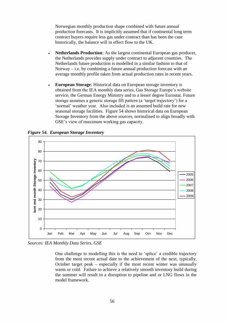
56
Norwegian monthly production shape combined with future annual
production forecasts. It is implicitly assumed that if continental long term
contract buyers require less gas under contract than has been the case
historically, the balance will in effect flow to the UK.
Netherlands Production: As the largest continental European gas producer,
the Netherlands provides supply under contract to adjacent countries. The
Netherlands future production is modelled in a similar fashion to that of
Norway – i.e. by combining a future annual production forecast with an
average monthly profile taken from actual production rates in recent years.
European Storage: Historical data on European storage inventory is
obtained from the IEA monthly data series, Gas Storage Europe‟s website
service, the German Energy Ministry and to a lesser degree Eurostat. Future
storage assumes a generic storage fill pattern (a „target trajectory‟) for a
„normal‟ weather year. Also included is an assumed build rate for new
seasonal storage facilities. Figure 54 shows historical data on European
Storage Inventory from the above sources, normalised to align broadly with
GSE‟s view of maximum working gas capacity.
Figure 54. European Storage Inventory
0
10
20
30
40
50
60
70
80
90
Jan Feb Mar Apr May Jun Jul Aug Sep Oct Nov Dec
bcm
en
d m
on
th S
tora
ge I
nven
tory
2005
2006
2007
2008
2009
Sources: IEA Monthly Data Series, GSE
One challenge to modelling this is the need to „splice‟ a credible trajectory
from the most recent actual date to the achievement of the next, typically,
October target peak – especially if the most recent winter was unusually
warm or cold. Failure to achieve a relatively smooth inventory build during
the summer will result in a disruption to pipeline and or LNG flows in the
model framework.

57
North American Storage Levels: In this conceptual framework we have
made the assertion that, as long as European Pipeline Import levels lie
somewhere between monthly minimum and maximum levels, a North
American storage level which is in line with a rolling average or a „market
expectation‟ for the month in question will equate to a Henry Hub price
which is converged with European Oil Indexed pipeline import prices. In a
future world where North America is reliant on LNG supplies above its
contractual minimum LNG volumes to meet demand and storage inventory
build this should be valid. For example, if storage inventory was marginally
lower than market expectations, bringing it back into line would require the
attraction of flexible LNG currently headed for Europe. Europe would be
happy to allow the redirection and back-fill with pipeline imports as long as
the price received for the LNG was just slightly higher than oil indexed
pipeline import prices. Conversely, if North American storage volumes
were slightly higher than market expectations, Europe would become
interested in attracting LNG away from North America and back out a
similar volume of more expensive oil-indexed pipeline gas. Qualifications
on this are firstly that incremental shipping costs could create a „dead band‟
of price – depending on the source of incremental LNG and, secondly, that
response times in „real life‟ are slower than „Excel‟(!) – such that a lag of
one or two months could be expected before this comes into play, with
onshore gas storage, regas tank inventory and floating LNG storage
providing the inventory buffer.
Figure 55. US Storage Surplus/Deficit and Atlantic Prices
0
2
4
6
8
10
12
14
16
Jan-
08
Feb-
08
Mar-
08
Apr-
08
May-
08
Jun-
08
Jul-
08
Aug-
08
Sep-
08
Oct-
08
Nov-
08
Dec-
08
Jan-
09
Feb-
09
$/m
mb
tu
-8,000
-6,000
-4,000
-2,000
-
2,000
4,000
6,000
8,000
Henry Hub
NBP
AGIP
US Storage Deficit/Surplus
Surp
lus
De
ficit
US
Sto
rag
e In
ve
nto
ry
Su
rplu
s/D
efi
cit
mm
cm
Sources: EIAi, Gas Matters, ICIS Heren
An illustration of the emergence of this effect is shown in Figure 55. In
early 2008 US storage inventory became depleted due to relatively cold
weather in 1Q – taking the dashed blue line above the blue axis. As the

58
storage deficit persisted, Henry Hub rose until by May and June it was on a
par with UK NBP and continental Europe Oil Indexed (AGIP) pipeline
prices. At the time there was some confusion in market sentiment regarding
the credibility of the most recent data on North American domestic
production which appeared to be growing more strongly than most observers
had predicted. Prior to the verification of this domestic production data
around mid year, it is suggested that the North American market in May and
June was anticipating the need to attract LNG from Europe in order to
reduce the storage deficit. Once the data on domestic production growth
was verified it became clear to the market that North America could easily
achieve its end injection season normal storage inventory levels without the
need to compete with Europe for additional LNG imports. In fact this was
comfortably achieved as Figure 55 shows, and Henry Hub prices de-linked
from European prices from July 2008 onwards.
Re-gas Capacity US and Europe: In Chapter 1 we examined the
considerable build in re-gas capacity earlier in this decade and asserted that
it was highly unlikely that this would constitute a barrier to LNG import
levels in the future.
LNG Supply Forecasts and Characteristics: Using monthly historical
data of LNG production by supplier and knowing their individual
liquefaction „nameplate‟ capacities it is possible to develop a monthly ratio
of LNG production to capacity at a supplier country level. Typically LNG
output is lower during the summer season (ambient temperature impacts the
operation of the liquefaction process) and maintenance periods will
obviously reduce output. For new trains coming on-stream a
„commissioning curve‟ can be assumed during initial ramp-up. Assuming
start-up dates for new liquefaction projects, a global LNG supply forecast
can be derived at a monthly level. This is examined quantitatively in
Appendix 2. Comparing the forecast with actuals reveals good agreement
apart from 2009. This is primarily due to underperformance by Nigeria and
Algeria who both claimed Force Majeure32
. This situation requires close
monitoring as the volumes (of around 20 bcma) would, if they had been
produced, have flowed to North America, broadly doubling LNG imports
there through most of 2009.
Apart from these apparent anomalies an LNG project, once it is operating
has a relatively low Short Run Marginal Cost of Supply. In large part this is
due to the tendency of LNG project developers to „segment‟ the supply
chain, creating different ownership entities for the upstream field
development, liquefaction train, shipping and regas terminals. Each segment
typically contracts for capacity with the next, on a „send or pay‟ contractual
basis. Once in operation there is a greatly reduced economic rationale for
shutting in production in response to low prices – as the only cost savings to
be made are probably the variable operating costs of the upstream fields
which are very low on a unit basis. The rational assumption therefore is that
once an LNG project is on-stream it will tend to continue to produce at
maximum rates. The situation in Nigeria and Algeria deserves monitoring
32
See Glossary for definition of Force Majeure

59
however to determine whether production is deliberately being withheld for
reasons other than short term economic rationale i.e. an anticipation of
greater revenues in the future if prices increase.
European minimum LNG imports: LNG and pipeline gas imports can be
interchanged across the European continent, as a direct exchange in Spain,
France and probably to a more limited extent in Italy, Greece and Turkey.
For NW Europe the UK acts as an intermediary importing more or less LNG
and connecting its spot gas supplies to the satellite trading hubs of North
West Europe via the Interconnector. At present we cannot quantify the
potential scale of the NW Europe connectivity available for this mechanism,
although the incentives would certainly emerge to expand transportation
capacity should such a bottleneck emerge. Accepting that connectivity may
be an issue we can apply a constraint to the model to force it to accept a
minimum quantity of LNG, based on historically observed minimum
monthly levels.
European LNG contract price: We have not directly addressed either the
contractual nature or oil-price indexation basis of much of the LNG
imported by Continental Europe. What we have done instead is to assume
that:
there is a minimum „must take‟ volume for Continental European
LNG Imports – reflecting a possible lack of connectivity and degree
of rigidity in some contracts which precludes cargo diversions.
generally there is sufficient flexibility in Atlantic Basin LNG
volumes to take advantage of arbitrage opportunities – as illustrated
in Figure 41.
pipeline take or pay obligations take precedence in terms of imports
into Europe. In a low demand period, if there is insufficient physical
storage to take contracted LNG take or pay volumes – they will be
diverted to North America albeit for a sales price lower than the
contracted price. Although this represents a marginal financial loss
it is better than paying for gas not taken at all.
This concludes the description of the conceptual model framework. Chapter 3 will use this
framework to understand the dynamics currently at play in the market and also to explore
the likely emerging trends and discontinuities.

60
3. Future Assumptions, Trends and Discontinuities Emerging
Introduction
This chapter takes the conceptual framework outlined in the previous chapter and, having
derived a credible assumption envelope for key variables, applies the framework to explore
key trends and discontinuities, primarily focussing on the Atlantic Basin arena.
Future Assumptions: Natural Gas Supply and Demand Fundamentals and LNG
Import Requirements
The future assumptions of national and regional demand, domestic production, pipeline
imports and LNG supply are discussed and set out in Appendix 2. This is not intended to
be an exhaustive derivation of future supply and demand forecasts. The main focus is on
the key uncertainties which will influence market dynamics in the medium to longer term.
Future Trends and Discontinuities Emerging from Modelling Framework
At this point, having developed our modelling framework and derived our initial set of
future assumptions in Appendix 2, we can look at the prognosis for future trends and
discontinuities.33
We will use a standardised set of graphics to examine the future in two time periods:
The period up to 2015;
The period to 2020.
The ‘Current Momentum’ Case
The first of three „futures‟ we will examine with the aid of the model framework is what we
call the „Current Momentum‟ Case. Essentially this is characterised by taking at face value
the future assumptions described in Appendix 2 and quantifying the outcome at a „whole
system‟ level.
The critical assumptions for this case are:
No significant near term reduction in North America domestic production.
Expansion of LNG supply on current start-up timings with no major outage
problems assumed post 2009. Apart from an assumed continuing 10 bcma
of „general underperformance‟ to mid 2011, it is assumed that LNG
producers do not deliberately hold back supply from the market.
Apart from an assumed 10% Take-or Pay rollover from contract year
October 08 – September 09, all European pipeline gas importers must
honour their take-or pay obligations (assumed at 85% of ACQ).
This set of assumptions, although quite widely held either individually or collectively,
results in an unsustainably oversupplied global system which does not have the
necessary storage capacity to cope.
Having demonstrated this, subsequent cases are developed to show how the system
could respond to accommodate the situation to 2015 and to 2020.
33
Although historical demand data was not available at the time of writing to cover the extremely cold month
of January 2010 in Europe and North America, the author has reflected this through an estimate.
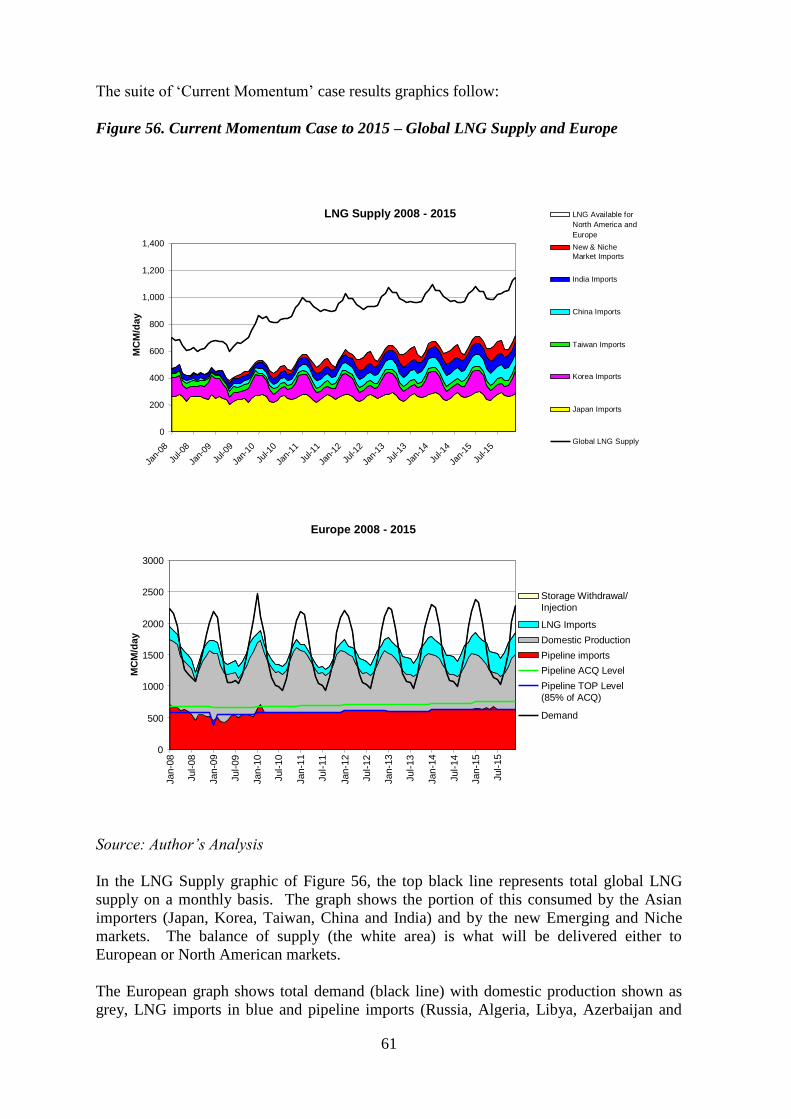
61
The suite of „Current Momentum‟ case results graphics follow:
Figure 56. Current Momentum Case to 2015 – Global LNG Supply and Europe
LNG Supply 2008 - 2015
0
200
400
600
800
1,000
1,200
1,400
Jan-
08
Jul-0
8
Jan-
09
Jul-0
9
Jan-
10
Jul-1
0
Jan-
11
Jul-1
1
Jan-
12
Jul-1
2
Jan-
13
Jul-1
3
Jan-
14
Jul-1
4
Jan-
15
Jul-1
5
MC
M/d
ay
LNG Available for
North America and
Europe
New & Niche
Market Imports
India Imports
China Imports
Taiwan Imports
Korea Imports
Japan Imports
Global LNG Supply
Europe 2008 - 2015
0
500
1000
1500
2000
2500
3000
Jan-0
8
Jul-
08
Jan-0
9
Jul-
09
Jan-1
0
Jul-
10
Jan-1
1
Jul-
11
Jan-1
2
Jul-
12
Jan-1
3
Jul-
13
Jan-1
4
Jul-
14
Jan-1
5
Jul-
15
MC
M/d
ay
Storage Withdrawal/
Injection
LNG Imports
Domestic Production
Pipeline imports
Pipeline ACQ Level
Pipeline TOP Level
(85% of ACQ)
Demand
Source: Author’s Analysis
In the LNG Supply graphic of Figure 56, the top black line represents total global LNG
supply on a monthly basis. The graph shows the portion of this consumed by the Asian
importers (Japan, Korea, Taiwan, China and India) and by the new Emerging and Niche
markets. The balance of supply (the white area) is what will be delivered either to
European or North American markets.
The European graph shows total demand (black line) with domestic production shown as
grey, LNG imports in blue and pipeline imports (Russia, Algeria, Libya, Azerbaijan and
62
Iran) in red. Storage injection and withdrawal volumes are shown as the semi-transparent
cream coloured layer. This graph of Europe shows a number of important features:
The January 2009 dip in pipeline imports are a consequence of the Russia-
Ukraine crisis.
The continuing low take of pipeline gas imports in 2009, (derived actuals to
end October 2009), leading to a 10% under-delivery on 1st October 2008 –
31st September 2009 contract year take or pay levels. Post 2009 it is
assumed that pipeline import take or pay levels are honoured at an assumed
85% of annual contract quantity. The model envisages Europe taking no
more than these levels until 2015 when there are occasional monthly imports
above these levels.
The lowered demand levels relative to 2008 and the adherence to pipeline
contract take or pay levels squeeze the import volumes of LNG to Europe
until 2012, when demand begins to noticeably recover.
We will revisit some of these assumptions to derive further cases.
Figure 57 shows the situation in North America where near term demand is depressed but
domestic production continues at around 2009 levels. The key dynamic here is the major
surge in LNG imports from January 2010 onwards, peaking in 2011 and then following a
diminishing trend to 2015.
The second graphic in Figure 57 shows the relative size of LNG imports into North
America and Europe. From early 2010 to the beginning of 2012, LNG supply surges into
North America as Europe has no physical room to absorb it, while honouring pipeline take
or pay commitments.
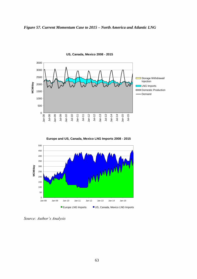
63
Figure 57. Current Momentum Case to 2015 – North America and Atlantic LNG
US, Canada, Mexico 2008 - 2015
0
500
1000
1500
2000
2500
3000
3500
Jan-0
8
Jul-
08
Jan-0
9
Jul-
09
Jan-1
0
Jul-
10
Jan-1
1
Jul-
11
Jan-1
2
Jul-
12
Jan-1
3
Jul-
13
Jan-1
4
Jul-
14
Jan-1
5
Jul-
15
MC
M/d
ay
Storage Withdrawal/
Injection
LNG Imports
Domestic Production
Demand
Europe and US, Canada, Mexico LNG Imports 2008 - 2015
0
50
100
150
200
250
300
350
400
450
500
Jan-08 Jan-09 Jan-10 Jan-11 Jan-12 Jan-13 Jan-14 Jan-15
MC
M/d
ay
Europe LNG Imports US, Canada, Mexico LNG Imports
Source: Author’s Analysis

64
Figure 58. Current Momentum Case to 2015 – North America Storage and Atlantic
Price Linkage
Atlantic Price Convergence/De-linkage - 2008 - 2015
-60
-40
-20
0
20
40
60
Jan-
08
Jul-
08
Jan-
09
Jul-
09
Jan-
10
Jul-
10
Jan-
11
Jul-
11
Jan-
12
Jul-
12
Jan-
13
Jul-
13
Jan-
14
Jul-
14
Jan-
15
Jul-
15
Pri
ce L
inkag
e/D
e-L
inkag
e
-80000
-60000
-40000
-20000
0
20000
40000
60000
80000
US
& C
an
ad
a S
tora
ge D
efi
cit
/Su
rplu
s
HH - AGIP De-Linkage HH & NBP - AGIP De-Linkage North America Surplus/Deficit mmcm
North America Storage Inventory - 2008 - 2015
-
50,000
100,000
150,000
200,000
250,000
300,000
350,000
Jan-0
8
May-0
8
Sep-0
8
Jan-0
9
May-0
9
Sep-0
9
Jan-1
0
May-1
0
Sep-1
0
Jan-1
1
May-1
1
Sep-1
1
Jan-1
2
May-1
2
Sep-1
2
Jan-1
3
May-1
3
Sep-1
3
Jan-1
4
May-1
4
Sep-1
4
Jan-1
5
May-1
5
Sep-1
5
MM
CM
en
d M
on
th
Storage Historic Range
Estimated Maximum
Storage Inventory
Henry Hub de-linked and
below Oil-Indexed Price
throughout period
Source: Author’s Analysis
The top graphic in Figure 58 shows North American storage inventory with the dotted red
line representing the maximum physical storage capacity. This confirms the unreality of
the „Current Momentum‟ case. Clearly, beyond mid 2010 it is not physically possible (from
a storage viewpoint) for North America to import the volumes of LNG represented here
and continue with domestic production at 2009 levels. The Atlantic price graph in Figure
58 represents (above the horizontal axis) the US & Canada storage surplus (blue line). The
yellow areas of the graph indicate that both Henry Hub and NBP are de-linked and lower
than the oil-indexed AGIP price. The red area indicates a period where NBP may be
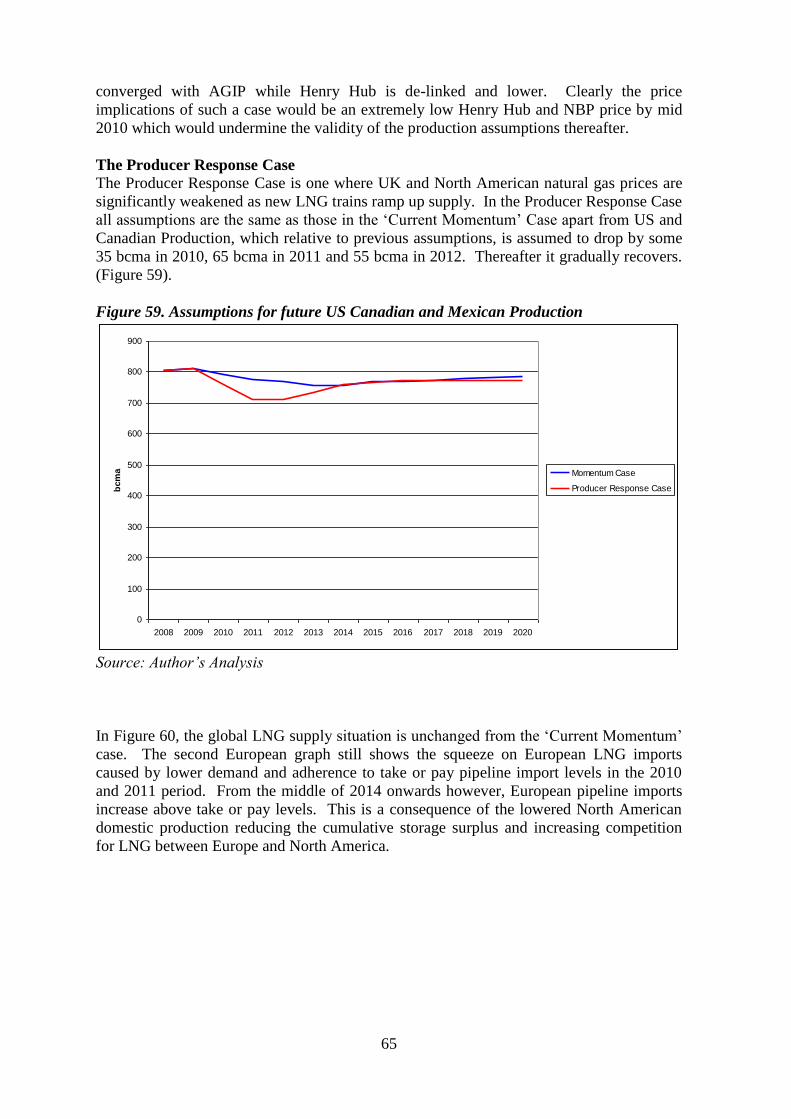
65
converged with AGIP while Henry Hub is de-linked and lower. Clearly the price
implications of such a case would be an extremely low Henry Hub and NBP price by mid
2010 which would undermine the validity of the production assumptions thereafter.
The Producer Response Case
The Producer Response Case is one where UK and North American natural gas prices are
significantly weakened as new LNG trains ramp up supply. In the Producer Response Case
all assumptions are the same as those in the „Current Momentum‟ Case apart from US and
Canadian Production, which relative to previous assumptions, is assumed to drop by some
35 bcma in 2010, 65 bcma in 2011 and 55 bcma in 2012. Thereafter it gradually recovers.
(Figure 59).
Figure 59. Assumptions for future US Canadian and Mexican Production
0
100
200
300
400
500
600
700
800
900
2008 2009 2010 2011 2012 2013 2014 2015 2016 2017 2018 2019 2020
bcm
a Momentum Case
Producer Response Case
Source: Author’s Analysis
In Figure 60, the global LNG supply situation is unchanged from the „Current Momentum‟
case. The second European graph still shows the squeeze on European LNG imports
caused by lower demand and adherence to take or pay pipeline import levels in the 2010
and 2011 period. From the middle of 2014 onwards however, European pipeline imports
increase above take or pay levels. This is a consequence of the lowered North American
domestic production reducing the cumulative storage surplus and increasing competition
for LNG between Europe and North America.

66
Figure 60. Producer Response Case to 2015 – Global LNG Supply and Europe
LNG Supply 2008 - 2015
0
200
400
600
800
1,000
1,200
1,400
Jan-
08
Jul-0
8
Jan-
09
Jul-0
9
Jan-
10
Jul-1
0
Jan-
11
Jul-1
1
Jan-
12
Jul-1
2
Jan-
13
Jul-1
3
Jan-
14
Jul-1
4
Jan-
15
Jul-1
5
MC
M/d
ay
LNG Available for
North America and
Europe
New & Niche
Market Imports
India Imports
China Imports
Taiwan Imports
Korea Imports
Japan Imports
Global LNG Supply
Europe 2008 - 2015
0
500
1000
1500
2000
2500
3000
Jan-0
8
Jul-
08
Jan-0
9
Jul-
09
Jan-1
0
Jul-
10
Jan-1
1
Jul-
11
Jan-1
2
Jul-
12
Jan-1
3
Jul-
13
Jan-1
4
Jul-
14
Jan-1
5
Jul-
15
MC
M/d
ay
Storage Withdrawal/
Injection
LNG Imports
Domestic Production
Pipeline imports
Pipeline ACQ Level
Pipeline TOP Level
(85% of ACQ)l
Demand
Source: Author’s Analysis

67
Figure 61. Producer Response Case to 2015 – North America and Atlantic LNG
US, Canada, Mexico 2008 - 2015
0
500
1000
1500
2000
2500
3000
3500
Jan-0
8
Jul-
08
Jan-0
9
Jul-
09
Jan-1
0
Jul-
10
Jan-1
1
Jul-
11
Jan-1
2
Jul-
12
Jan-1
3
Jul-
13
Jan-1
4
Jul-
14
Jan-1
5
Jul-
15
MC
M/d
ay
Storage Withdrawal/
Injection
LNG Imports
Domestic Production
Demand
Europe and US, Canada, Mexico LNG Imports 2008 - 2015
0
50
100
150
200
250
300
350
400
450
500
Jan-08 Jan-09 Jan-10 Jan-11 Jan-12 Jan-13 Jan-14 Jan-15
MC
M/d
ay
Europe LNG Imports US, Canada, Mexico LNG Imports
Source: Author’s Analysis
The North America graphic in Figure 61 shows the lowered domestic production „making
room‟ for substantially higher LNG volumes throughout the period with some reduction by
2015 as domestic production recovers.

68
The LNG graphic in Figure 61 again shows the near term surge of LNG into North
America as Europe is unable to take high levels of LNG and at the same time honour its
pipeline import take or pay quantities.
Figure 62. Producer Response Case to 2015 – North America Storage and Atlantic Price
Linkage
Atlantic Price Convergence/De-linkage - 2008 - 2015
-60
-40
-20
0
20
40
60
Jan-
08
Jul-
08
Jan-
09
Jul-
09
Jan-
10
Jul-
10
Jan-
11
Jul-
11
Jan-
12
Jul-
12
Jan-
13
Jul-
13
Jan-
14
Jul-
14
Jan-
15
Jul-
15
Pri
ce L
inkag
e/D
e-L
inkag
e
-80000
-60000
-40000
-20000
0
20000
40000
60000
80000
US
& C
an
ad
a S
tora
ge D
efi
cit
/Su
rplu
s
HH - AGIP De-Linkage HH & NBP - AGIP De-Linkage North America Surplus/Deficit mmcm
North America Storage Inventory - 2008 - 2015
-
20,000
40,000
60,000
80,000
100,000
120,000
140,000
160,000
180,000
Jan-0
8
May-0
8
Sep-0
8
Jan-0
9
May-0
9
Sep-0
9
Jan-1
0
May-1
0
Sep-1
0
Jan-1
1
May-1
1
Sep-1
1
Jan-1
2
May-1
2
Sep-1
2
Jan-1
3
May-1
3
Sep-1
3
Jan-1
4
May-1
4
Sep-1
4
Jan-1
5
May-1
5
Sep-1
5
MM
CM
en
d M
on
th
Storage Historic Range
Estimated Maximum
Storage Inventory
Henry Hub de-linked and
below Oil-Indexed Price
through to 2015
Source: Author’s Analysis
The North American storage graphic in Figure 62 still shows modelled storage inventory
levels in excess of physical available capacity during 2010 and 2011. From 2012 onwards

69
however, we see signs that the system is tightening and by 2014 the modelled storage
inventory level is within the historical minimum – maximum range.
The blue trend on the price indicator graph in Figure 62 tracks this surplus/deficit position.
The prognosis is that both NBP and Henry Hub prices would be de-linked and below AGIP
to the beginning of 2015. During 2015 there is a storage deficit although probably not
sufficient to cause a major escalation of Henry Hub and NBP above oil-indexed price level.
Although the „Producer Response‟ case has reduced the imbalances seen in the „Current
Momentum‟ case it still strays beyond the boundaries of what is manageable with current
North American storage capacity.
The European Contract Flexibility Case
The Producer Response case represents a continuation, to mid 2014, of the difficult
circumstances that importers of oil-indexed pipeline gas have found themselves in since
early 2009. Prices for spot gas on trading hubs, for much of 2009 were about half the price
of oil-indexed pipeline imports. Oil-indexed gas importers have had difficulty meeting
take-or-pay obligations due to loss of end-user demand to competing spot gas, and may
well be facing three painful choices:
Pay for take or pay gas quantities but not physically take all of it, thus
incurring significant financial loss. (Note: We have assumed in this
framework that 10% of the 2009 contract year gas is „rolled over‟ for
physical delivery in the next or future contract year(s).
Pay for take or pay gas quantities, take the full physical quantity and
mitigate the financial loss by re-selling it on a traded hub at spot prices. At
2009 gas prices this would halve the loss but would still be substantial. If
the „home market demand‟ for these mid stream buyers has been reduced
both by the recession and by competing spot gas volumes the issue may then
become whether infrastructure connectivity is sufficient to allow the balance
of the TOP volume to be sold out on national hubs without further
drastically reducing those prices.
Re-negotiate downward flexibility in TOP levels to reduce the financial
exposure. This of course directly impacts the revenue of upstream sellers
and only the prospect of the financial collapse of a buyer as a „long term
strategic partner‟ is likely to result in such an outcome.
In the European Contract Flexibility case, we allow TOP volumes to be reduced from the
base assumption of 85% of annual contract quantity down to 70% from October 2009 to the
end of September 2012.
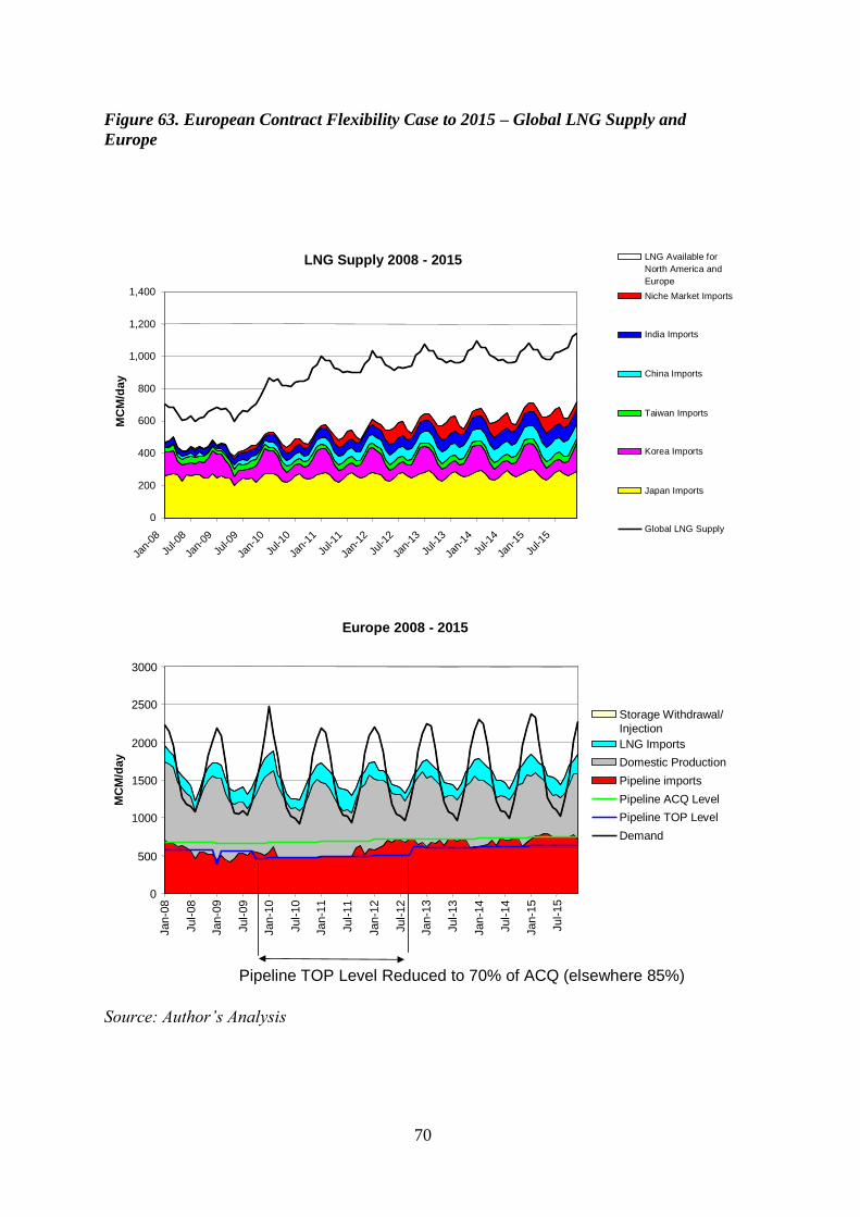
70
Figure 63. European Contract Flexibility Case to 2015 – Global LNG Supply and
Europe
LNG Supply 2008 - 2015
0
200
400
600
800
1,000
1,200
1,400
Jan-
08
Jul-0
8
Jan-
09
Jul-0
9
Jan-
10
Jul-1
0
Jan-
11
Jul-1
1
Jan-
12
Jul-1
2
Jan-
13
Jul-1
3
Jan-
14
Jul-1
4
Jan-
15
Jul-1
5
MC
M/d
ay
LNG Available for
North America and
Europe
Niche Market Imports
India Imports
China Imports
Taiwan Imports
Korea Imports
Japan Imports
Global LNG Supply
Europe 2008 - 2015
0
500
1000
1500
2000
2500
3000
Jan-0
8
Jul-
08
Jan-0
9
Jul-
09
Jan-1
0
Jul-
10
Jan-1
1
Jul-
11
Jan-1
2
Jul-
12
Jan-1
3
Jul-
13
Jan-1
4
Jul-
14
Jan-1
5
Jul-
15
MC
M/d
ay
Storage Withdrawal/
Injection
LNG Imports
Domestic Production
Pipeline imports
Pipeline ACQ Level
Pipeline TOP Level
Demand
Pipeline TOP Level Reduced to 70% of ACQ (elsewhere 85%)
Source: Author’s Analysis
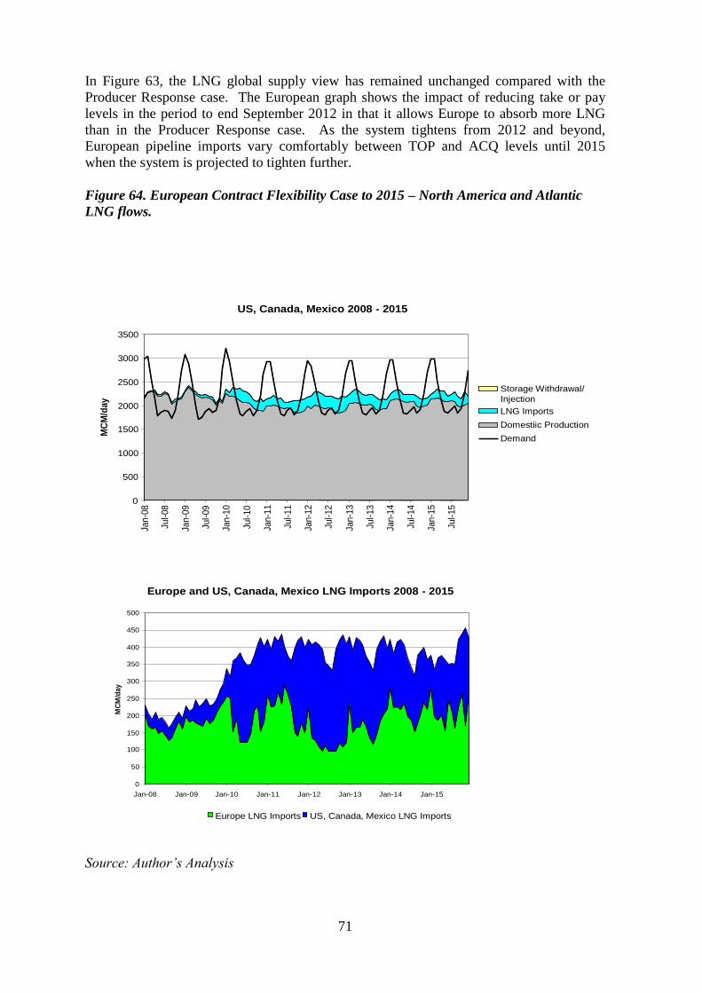
71
In Figure 63, the LNG global supply view has remained unchanged compared with the
Producer Response case. The European graph shows the impact of reducing take or pay
levels in the period to end September 2012 in that it allows Europe to absorb more LNG
than in the Producer Response case. As the system tightens from 2012 and beyond,
European pipeline imports vary comfortably between TOP and ACQ levels until 2015
when the system is projected to tighten further.
Figure 64. European Contract Flexibility Case to 2015 – North America and Atlantic
LNG flows.
US, Canada, Mexico 2008 - 2015
0
500
1000
1500
2000
2500
3000
3500
Jan-0
8
Jul-
08
Jan-0
9
Jul-
09
Jan-1
0
Jul-
10
Jan-1
1
Jul-
11
Jan-1
2
Jul-
12
Jan-1
3
Jul-
13
Jan-1
4
Jul-
14
Jan-1
5
Jul-
15
MC
M/d
ay
Storage Withdrawal/
Injection
LNG Imports
Domestiic Production
Demand
Europe and US, Canada, Mexico LNG Imports 2008 - 2015
0
50
100
150
200
250
300
350
400
450
500
Jan-08 Jan-09 Jan-10 Jan-11 Jan-12 Jan-13 Jan-14 Jan-15
MC
M/d
ay
Europe LNG Imports US, Canada, Mexico LNG Imports
Source: Author’s Analysis

72
In North America although there is still a surge in LNG imports in Figure 64, it is not as
severe as in the Producer Response Case. The North America and Europe LNG import
chart shows Europe maintaining much higher LNG import levels in 2011.
Figure 65. European Contract Flexibility Case to 2015 – North America Storage and
Atlantic Price Linkage.
Atlantic Price Convergence/De-linkage - 2008 - 2015
-60
-40
-20
0
20
40
60
Jan-
08
Jul-
08
Jan-
09
Jul-
09
Jan-
10
Jul-
10
Jan-
11
Jul-
11
Jan-
12
Jul-
12
Jan-
13
Jul-
13
Jan-
14
Jul-
14
Jan-
15
Jul-
15
Pri
ce L
inkag
e/D
e-L
inkag
e
-80000
-60000
-40000
-20000
0
20000
40000
60000
80000
US
& C
an
ad
a S
tora
ge D
efi
cit
/Su
rplu
s
HH - AGIP De-Linkage HH & NBP - AGIP De-Linkage North America Surplus/Deficit mmcm
North America Storage Inventory - 2008 - 2015
-
20,000
40,000
60,000
80,000
100,000
120,000
140,000
160,000
Jan-0
8
May-0
8
Sep-0
8
Jan-0
9
May-0
9
Sep-0
9
Jan-1
0
May-1
0
Sep-1
0
Jan-1
1
May-1
1
Sep-1
1
Jan-1
2
May-1
2
Sep-1
2
Jan-1
3
May-1
3
Sep-1
3
Jan-1
4
May-1
4
Sep-1
4
Jan-1
5
May-1
5
Sep-1
5
MM
CM
en
d M
on
th
Storage Historic Range
Estimated Maximum
Storage Inventory
Henry Hub de-linked and
below Oil-Indexed Price
through to 2012Henry Hub mainly converged
with Oil-Indexed Price
Henry Hub de-linked and
slightly above oil-indexed
prices
Source: Author’s Analysis

73
In the European Contract Flexibility case the North American storage position is
manageable although in 2012 and 2015 there are modest deficits (Figure 65). The price
graphic shows that in the period 2012 to 2015, there is likely to be general convergence
between Henry Hub, NBP and AGIP with the prospect of the spot prices de-linking and
rising above AGIP/residual fuel oil by the end of 2015, although probably not significantly.
The Longer Term
This section looks at the period to 2020 on this European Contract Flexibility Case.
Figure 66. European Contract Flexibility Case to 2020 – Global LNG Supply and
Europe
LNG Supply 2008 - 2020
0
200
400
600
800
1,000
1,200
1,400
1,600
1,800
Jan-0
8
Jan-0
9
Jan-1
0
Jan-1
1
Jan-1
2
Jan-1
3
Jan-1
4
Jan-1
5
Jan-1
6
Jan-1
7
Jan-1
8
Jan-1
9
Jan-2
0
MC
M/d
ay
LNG Available for
North America and
Europe
Niche Market Imports
India Imports
China Imports
Taiwan Imports
Korea Imports
Japan Imports
Global LNG Supply
Europe 2008 - 2020
0
500
1000
1500
2000
2500
3000
Jan-0
8
Jan-0
9
Jan-1
0
Jan-1
1
Jan-1
2
Jan-1
3
Jan-1
4
Jan-1
5
Jan-1
6
Jan-1
7
Jan-1
8
Jan-1
9
Jan-2
0
MC
M/d
ay
Storage Withdrawal/
Injection
LNG Imports
Domestic Production
Pipeline imports
Pipeline ACQ Level
Pipeline TOP Level
Demand
Pipeline TOP Level Reduced to 70% of ACQ (elsewhere 85%)
Source: Author’s Analysis

74
The LNG supply graphic in Figure 66 shows the growth of the next „wave‟ of new projects,
significantly those in Nigeria and Australia in the 2015 - 2020 timeframe.
The European graphic in Figure 67 shows domestic production noticeably in decline post
2015 while LNG imports are steadily increasing. Pipeline import levels vary between take
or pay and annual contract quantity levels generally throughout the period post 2012.
Figure 67. European Contract Flexibility Case to 2020 – North America and Atlantic
LNG Flows
US, Canada, Mexico 2008 - 2020
0
500
1000
1500
2000
2500
3000
3500
Jan-0
8
Jan-0
9
Jan-1
0
Jan-1
1
Jan-1
2
Jan-1
3
Jan-1
4
Jan-1
5
Jan-1
6
Jan-1
7
Jan-1
8
Jan-1
9
Jan-2
0
MC
M/d
ay
Storage Withdrawal/
Injection
LNG Imports
Domestic Production
Demand
Europe and US, Canada, Mexico LNG Imports 2008 - 2020
0
100
200
300
400
500
600
700
800
Jan-
08
Jan-
09
Jan-
10
Jan-
11
Jan-
12
Jan-
13
Jan-
14
Jan-
15
Jan-
16
Jan-
17
Jan-
18
Jan-
19
Jan-
20
MC
M/d
ay
Europe LNG Imports US, Canada, Mexico LNG Imports
Source: Author’s Analysis

75
In North America, LNG imports in Figure 67 remain high in historical terms even as
Europe significantly increases LNG imports beyond 2015 to offset its declining domestic
production and to meet demand growth.
Figure 68. European Contract Flexibility Case to 2020 – North American Storage and
Atlantic Price Linkage
Atlantic Price Convergence/De-linkage - 2008 - 2020
-60
-40
-20
0
20
40
60
Jan-
08
Jan-
09
Jan-
10
Jan-
11
Jan-
12
Jan-
13
Jan-
14
Jan-
15
Jan-
16
Jan-
17
Jan-
18
Jan-
19
Jan-
20
Pri
ce L
inkag
e/D
e-L
inkag
e
-80000
-60000
-40000
-20000
0
20000
40000
60000
80000
US
& C
an
ad
a S
tora
ge D
efi
cit
/Su
rplu
s
HH - AGIP De-Linkage HH & NBP - AGIP De-Linkage North America Surplus/Deficit mmcm
North America Storage Inventory - 2008 - 2020
-
20,000
40,000
60,000
80,000
100,000
120,000
140,000
160,000
Jan-0
8
Jan-0
9
Jan-1
0
Jan-1
1
Jan-1
2
Jan-1
3
Jan-1
4
Jan-1
5
Jan-1
6
Jan-1
7
Jan-1
8
Jan-1
9
Jan-2
0
MM
CM
en
d M
on
th
Storage Historic Range
Estimated Maximum
Storage Inventory
Henry Hub de-linked and
below Oil-Indexed Price
through to 2012Henry Hub mainly converged
with Oil-Indexed Price
Henry Hub de-linked and
slightly above oil-indexed
prices
Source: Author’s Analysis

76
And finally, after a mildly „tight‟ market around the middle of the next decade, North
American storage inventory in Figure 68 remains broadly in line with historic average
levels. This is reflected in the price graph in Figure 68 which shows Henry Hub and NBP
converged post 2015.
It must be stressed that the results of the European Contract Flexibility case are a direct
consequence of the underlying global supply and demand assumptions. If these change
significantly, this could very easily result in a less balanced system. The purpose of
presenting these graphs however is to illustrate the way in which the new „LNG-connected‟
system dynamics transmit prices and physical flows between regions.
The key dynamic illustrated here has been the system response to an „oversupply‟ situation
caused by a „perfect storm‟ combination of:
high US and Canadian production due to the growth of unconventional gas,
reduced demand for natural gas caused by the economic recession,
the surge in LNG supply from new projects sanctioned in the early to mid
2000s.
The instability thus created has been absorbed by a combination of a price-driven reduction
in North American production and a temporary, although significant, additional flexibility
in European pipeline minimum contract volume take or pay requirements.
Whether North American production dynamics and response times will behave in the way
assumed in this analysis is a key uncertainty. For example, if North American production
remains resilient despite low prices this would place greater strain on the ability of
Europe‟s oil indexed pipeline importers to sell-on their contractual minimum volumes. An
effective take or pay level lower than the 70% level used here would be necessary.
When demand recovers, a slower build-up of North American production than that
assumed here would lead to an „overshoot‟ taking Henry Hub and NBP prices above those
of oil-indexed prices. This leads to a more general question of the ability of „shorter lead-
time‟ supplies (e.g. North American gas) to respond and adjust to sudden increases in
supply from „longer lead time‟ sources such as LNG.

77
4. Conclusions
In the period spanning 2000 to 2009 the global gas system has changed from being
comprised of individual national or regional markets to one where inter-regional tradeflows
have a noticeable impact on both the physical supply-demand dynamics, and in some
circumstances prices.
It is overly simplistic and at best premature to claim that the growth in LNG supply since
2005 has created a „global market for natural gas‟. The low energy density of natural gas
(in gaseous form) compared with oil and oil products leads to a requirement for far greater
investment in gas transportation and storage infrastructure per unit of energy. This
characteristic of the natural gas supply chain, as much as contractual constraints, will exert
a dampening effect on the logical momentum towards a truly liquid global market (in the
same sense as the global oil market) for this commodity.
This said, the changes which have taken place since 2000 have set the scene for new
dynamics which will re-characterise the supply and pricing patterns in many countries and
regions which import, or are about to import, significant quantities of natural gas. In this
respect the key „enabling‟ structural changes since 2000 are:
The need (or perceived need) and capability for the liberalised markets of North
America and the UK to import significant quantities of future LNG – pricing off
domestic market trading hubs.
The undermining of „destination‟ clauses in the European market by EU competition
rules.
The underperformance of Indonesia as an exporter of LNG to Asian markets and the
delay of contracted supply from new LNG projects.
The increased willingness of LNG buyers and sellers, driven by short term „enlightened
self interest‟ to introduce flexibility into their contractual arrangements and share the
additional profit margin afforded by LNG arbitrage.
These structural changes have driven the following „behavioural‟ changes or challenges to
the various regional markets:
In response to the Indonesian underperformance and project delays, Asian markets
resorted to the purchase of spot or short term supply. In the 2009 demand downturn
some (Japan, Korea, Taiwan) were allegedly seeking to reduce imports below
contractual minima.
In Europe the phase out of destination clauses has weakened the linkage which enabled
a national market incumbent to match forecast national demand with contracted supply.
While behavioural inertia and cross-border infrastructure capacity constraints will
constrain the pace of change, the future is likely to be characterised by the need to
contract new supplies for the European market in aggregate. This carries inherently
more forecasting risk, especially when contracted supply may be in competition with
spot supply at traded hubs.
In North America and the UK, actual or perceived tightening of supply relative to
demand has led to the development of new import projects, especially those involving
LNG. Uncertainty in predicting both domestic demand and supply beyond the current
year sits uneasily with the need to gauge the timing and scale of investment in new
LNG projects which have a lead time of 4 - 5 years.

78
Thus we now have a „system‟ of natural gas markets which to varying degrees are linked
by LNG supply, comprising the Asian markets of Japan, Korea, Taiwan, China and India,
the European Region and North America. Their aggregate annual natural gas consumption
amounts to some 1,600 bcm.
The framework developed in this paper, based on observed dynamics to date and the
combination of contractual mechanics and LNG arbitrage response:
assumes that the Asian Markets will continue to import the volumes of LNG they
require to meet domestic consumption even where this requires paying premium spot
market prices. There is an inherent uncertainty in forecasting the LNG import needs of
China and India given their demand growth upside and the scale and timing of future
domestic production and pipeline imports, but for the next year or so, LNG imports are
bounded on the upside by known re-gas capacity limits.
accounts for the anticipated volumes of LNG destined for new „niche‟ markets leaving
the LNG supply available for Europe and North America. Given the very low short run
marginal costs of supply for LNG projects it is assumed that LNG production will not
be curtailed in response to price, at least for economic reasons.
models the Atlantic Basin LNG dynamic as a function of the interaction of oil-indexed
pipeline gas imports into European markets (from Russia, Algeria, Libya, Azerbaijan
and Iran) and LNG – pricing at the margin off North American traded prices:
From a starting point of North American prices being lower than European
pipeline import oil-indexed prices, one would expect European importers to
lower their nomination of pipeline gas and attract more, cheaper, LNG. The net
effect is to reduce supply to North America where prices respond to the
changing levels of storage inventory. This process would continue until either:
North American prices had risen to converge with European oil indexed
prices at which point the arbitrage would cease; or,
European pipeline imports would reach the seasonally adjusted „take or
pay‟ levels and could fall no further. Thus North American prices would
remain below European oil indexed prices.
From a starting point of North American prices being higher than European oil-
indexed import prices, one would expect European importers to increase their
nomination of cheaper pipeline gas and divert more LNG to North America to
take advantage of the higher price. The net effect is to increase supply to North
America where prices would respond to the changed level of storage inventory.
This process would continue until either:
North American prices had fallen to converge with European oil indexed
prices at which point the arbitrage would cease; or,
European pipeline imports would reach the seasonally adjusted „contract
quantity‟ levels and could rise no further. Thus North American prices
would remain above European Oil Indexed prices.
recognises the additional „real world‟ constraints of LNG contractual flexibility and
infrastructure. The above dynamic is bounded by a minimum level of European and
North American LNG imports. Another qualification is that while using the term „price
convergence‟ across the Atlantic Basin, there would in fact be a price differential,
equivalent to the incremental LNG shipping cost between Europe and North America
which is of the order of $0.40/mmbtu in 2009. Provided that North America was
importing more than its observed minimum LNG quantity we would expect the UK
price to follow that of North America, subject to the differential LNG shipping cost.

79
From a „systems‟ perspective, the above dynamic represents a means by which the new
„global system‟, albeit comprising regional markets of differing structures and behavioural
drivers, seeks to balance supply and demand through price signals and arbitrage. The use
of the flexibility band in Europe‟s long term pipeline gas import contracts is a means of
physically adding or removing gas from the system i.e. literally by altering upstream
production levels. However the scope of this physical adjustment is relatively minor in
scale. In annualised terms the flexibility in contractual take amounts to only some 40 bcma
in an aggregated LNG-connected natural gas market of 1,600 bcma. Accepting the
hypothesis that in the future „getting supply levels right‟ will be more difficult than in the
past, it is likely that there will be periods where the system will veer out of balance by more
than the 40 bcma pipeline contract „cushion‟.
Following the logic developed above and noting other observed dynamics in the paper we
can describe the characteristics and response mechanisms of a „very tight‟ and a „very
loose‟ supply-demand world as follows:
The ‘very tight’ world would be one where despite European pipeline levels being at their
contractual maxima throughout the year, North American (and UK) prices were higher than
oil indexed European prices. The following response sequence would seek to redress the
situation:
North American gas storage inventory would be reduced to below average
levels for the specific month in question.
In North America as natural gas price rises above that of residual fuel oil one
would expect to see fuel switching come into effect. Depending on the level of
switching capacity maintained in the future, one would expect this switching
band to progressively reduce gas demand by some 15 to 20 bcma. This
response would be relatively rapid.
If North American prices remained at or above residual fuel parity for several
months one would expect to see an increase in gas drilling intensity – with a
domestic supply response within say 12 months.
If the upstream industry expected North American and UK prices to remain
high for the foreseeable future then one would expect to see increased focus on
developing new longer lead time supply (4 to 5 years), such as:
New LNG projects in Nigeria, Australia and potentially Qatar (assuming
the lifting of the moratorium on the North Field).
Unconventional gas production in Europe.
On the demand side, sustained high prices in North America and the UK would
exacerbate the trend of „demand relocation‟ of gas intensive industries to
countries where prices are lower, often due to state subsidy or regulation.
In time the response mechanisms above would bring the system back to a point where
the European – North American pipeline – LNG arbitrage dynamic would again
provide the price-driven balancing mechanism.
The ‘very loose’ world would be one where despite European pipeline levels being at their
contractual minima throughout the year, North American (and UK) prices were lower than
oil indexed European prices. The following response sequence would seek to redress the
situation:
North American gas storage inventory would increase to above average levels
for the specific month in question, within end - October physical limits.

80
In North America (and the UK) as natural gas price competes with coal in
power generation, one would expect to see switching from coal to gas come into
effect. This response would be relatively rapid.
If North American prices remained at or below the economic cost of supply of
domestic production for several months one would expect to see a decrease in
gas drilling intensity – with a domestic supply response within say 12 months.
If the upstream industry expected North American and UK prices to remain low
for the foreseeable future then one would expect to see a deferral of new longer
lead time supply (4 to 5 years), such as new LNG projects.
On the demand side, sustained low prices in North America and the UK might
alleviate the trend of „demand relocation‟ of gas intensive industries to countries
where prices are low, often due to state subsidy or regulation.
In time the response mechanisms above would bring the system back to a point where
the European – North American pipeline – LNG arbitrage dynamic would again
provide the price-driven balancing mechanism.
Clearly at the end of 2009 the system is in the „very loose‟ state and most of the corrective
mechanisms listed above are in play to bring it back into a position of balance where the
European – North American pipeline – LNG arbitrage dynamic will resume as the
balancing mechanism. The timing of the rebalancing dynamic will also be impacted by the
following specific factors:
The rate at which natural gas demand growth resumes during the post – recession
economic recovery period.
The trajectory of domestic North American production as a key balancing force.
Production shut-in could be forced by low prices and constrained storage capacity
during 2010.
The emerging period of net decline in European domestic production from 2012
onwards as Norwegian production reaches a plateau.
The limited scope for growth in additional pipeline imports to Europe post 2012.
The impact of deferral of future LNG projects – resulting in lower growth in global
LNG supply from around 2012.
The expectation is for a tightening of the system by 2012 - 2013.
In the immediate future the following responses have been postulated and modelled to
illustrate what is required to keep this „system‟ within the bounds of physical reality, given
the surplus of imminent supply relative to demand. These responses include:
A reduction in North American domestic production of the order of 7 to 8 %
in 2011-2012 compared with 2009 levels.
A relaxation of European pipeline import contract take or pay levels from
85% of Annual Contract Quantity down to 70% from October 2009 to end
September 2012.
The dynamics of the system described in this paper will be plain to observe given the
occurrence of the „perfect storm‟ which is currently impacting this system:
an unforeseen high level of US domestic production.
demand levels below those anticipated due to the economic recession,

81
since October 2009, the huge growth in LNG supply, much of which is
inherently destination flexible or „self contracted‟,
The combination of assumptions used in the analysis in this paper have resulted in a
modelled outcome where the system recovers its balance by 2012 and remains stable to
2020, with traded prices generally converging on oil-indexed price levels post 2012. Given
the uncertainties in many of the assumptions, it is equally possible that the dynamics of this
new global system, given the relatively long lead times of significant tranches of new
supply remote from importing markets would imply a succession of cycles rather than the
achievement of a stable converged global system. This would also have significant
implications for price volatility in the liberalised markets of North America and the UK
with periodic enhanced trading opportunities at hubs on the interface of oil-indexed and
liberalised market „blocs‟.

82
5. Appendix 1 : Models of LNG Arbitrage
Polina Zhuravleva34
describes four models of LNG arbitrage and three examples of short
term sales which fall short of a strict definition of arbitrage. The following description is an
extract from her paper. All the true arbitrage models assume that the Seller1 of the LNG
has a contract (whether it is a long-term, short-term or even a spot contract) with the Initial
Buyer and is obliged to supply a cargo on these terms at a fixed date.
Model 1 – Seller Arbitrageur
The first model (Figure A1.1), implies that the Seller initiates the arbitrage and takes the
role of arbitrageur. The Seller, who has a contract with the Initial Buyer to deliver the LNG
cargo on day N, sees the opportunity to sell this cargo in another market and acquire the
margin. The Seller may offer the Initial Buyer the chance to forfeit the deal and share the
margin. The diverted LNG cargo may have to be replaced by an equivalent quantity of gas
from the LNG Spot Market, from domestic production or from pipeline imports. If the
price differentials are high enough to cover transaction costs, the arbitrage deal is viable.
The split of the profits is agreed between the contracting parties. In this example, the Initial
Buyer has a veto over the destination of the cargo and can refuse to agree to the diversion.
Figure A1.1 – Model 1 : Seller-Arbitrageur
Initial B uyer of
L NG
Initial B uyer of
L NG
E nd B uyer of L NG
E nd B uyer of L NG
S eller of L NG
S eller of L NG
•L NG S pot Market•L ocal G as Market•Other S ources
•L NG S pot Market•L ocal G as Market•Other S ources
L NG *
Trans fer of the volume ris k* This graphic doesn’t s how phys ical movement of the cargo
S plit of P rofit
F orfeits the Deal
L NG R eplacement
Model I: L NG S eller Ac ts As Arbitrag eur
34
The Nature of LNG Arbitrage, and an Analysis of the Main Barriers for the Growth of the Global LNG
Arbitrage Market, OIES, July 2009.

83
Figure A1.2 – Initial Buyer - Arbitrageur
Initial B uyer of
L NG
Initial B uyer of
L NG
E nd B uyer of L NG
E nd B uyer of L NG
S eller of L NG
S eller of L NG
•L NG S pot Market•L ocal G as Market•Other S ources
•L NG S pot Market•L ocal G as Market•Other S ources
L NG R eplacement
L NG *
Trans fer of the volume ris k* This graphic doesn’t s how phys ical movement of the cargo
S plit of P rofit
Model II: Initial B uyer Ac ts As Arbitrag eur
In this model (Figure A1.2), the Initial Buyer decides to divert the cargo to a market that
offers a higher price. There can be two reasons why the Initial Buyer decides to divert
the LNG vessel: first, the cargo can be replaced by cheaper gas from domestic production,
from cheaper pipeline gas imports or by LNG from the spot market; or, simply, the buyer
might not physically need the cargo. If contractual clauses allow cargo diversion (or if it
was agreed with the seller), the Initial Buyer sends the cargo to the End Buyer and, in most
cases, has to split the margin with the Seller. If replacement of the diverted cargo is
required, it is the Initial Buyer‟s responsibility. If a destination clause is incorporated into
the LNG contract, arbitrage by the Initial Buyer will be restricted.

84
Figure A1.3 - Independent Trader-Arbitrageur
Initial B uyer of
L NG
Initial B uyer of
L NG
Indepen-dent
Trader
Indepen-dent
Trader
E nd B uyer of L NG
E nd B uyer of L NG
S eller of L NG
S eller of L NG
•L NG S pot Market•L ocal G as Market•Other S ources
•L NG S pot Market•L ocal G as Market•Other S ources
L NG R eplacement
L NG *
Trans fer of the volume ris k* This graphic doesn’t s how phys ical movement of the cargo
Model III: Independent T rader Ac ts As Arbitrag eur
In this model (Figure A1.3), another player appears in the transaction – the Independent
Trader. An Independent Trader buys the cargo from the Initial Buyer (seldom from LNG
Seller) or gets the right to divert the cargo to another customer offering a higher price.
Whether the participants split the profit depends on the individual agreements and varies
from case to case. If replacement of the diverted cargo is required, it also depends on the
agreement whether the Initial Buyer or an Independent Trader will replace it.
Model 4 - LNG Reloading
LNG Reloading has been used at Huelva terminal in Spain and at the Zeebrugge LNG
terminal. This is a relatively new category of cargo diversion and implies a purchase of the
LNG cargo, discharge from the vessel into the storage tank and a subsequent reloading into
another ship. This enables terminal users at to ship the cargoes to other markets and take
advantage of price differentials. In the case of Zeebrugge the contractual destination
clauses preclude diversions of the LNG; but the cargoes are delivered under DES
(Delivered Ex-Ship) arrangement. Once the cargo is discharged into the Zeebrugge storage
tanks, its title passes to the terminal capacity user (GdF Suez, Electricite de France or
Distrigas). This allows re-export of the LNG without violating the contract and avoids
profit sharing with the initial LNG seller. The reloaded LNG is diverted to higher priced
markets, thus acting as a „market balancing force‟; and so it can be regarded as arbitrage.
Non-Arbitrage Short Term LNG Transactions
The following are examples of short term LNG transactions which would not normally fit a
definition of arbitrage, i.e. that the transaction was motivated by price differentials between
the markets and thus contributes to arbitrage equilibrium.

85
Physical LNG Cargo Swaps
Figure A1.4 Physical LNG Cargo Swaps
S eller:Trinidad & Tobago
S eller:Trinidad & Tobago
B uyer: S pain
B uyer: S pain
B uyer:US A
B uyer:US A
S eller: Algeria
S eller: Algeria
Delivery according the initial contract
C argo s wap
C ontrovers ial L NG R edirec tions
1. P hys ic al C arg o S wap
2. L NG R eloading (e.g . Z eebrug g e) Terminal’s c apac ity is des ig ned to dis c harg e L NG from the s hip, s tore it and reload on another ves s el G as pric e c onvers ion
Figure A1.4 shows an example of two cargoes that are located in different countries (e.g.
Trinidad and Tobago and Algeria). In accordance with the contract the Algerian cargo is
allotted to the USA, while the cargo from Trinidad and Tobago is committed to Spain. In
order to reduce transportation costs and possible taxes (or, in some cases, the costs for LNG
quality management) the parties decide to swap the cargos and share the resulting profit.
However, this profit arises from cost minimization, not from exploiting price differentials.
Therefore this type of LNG redirection does not lead to price convergence and does not
comply with the definition of arbitrage.

86
Portfolio Optimisation
Figure A1.5 Portfolio Optimisation
C ompany X
C ompany X
Market AMarket A
Market BMarket B
Market CMarket C
L NG C argo
L NG P lant
L NG C argo
L NG C argo
L NG P lant
L NG P lant
L NG P ortfolio Optimization
•B uyer-S eller model•No price convers ion (if the L NG volume is about the s ame)•C os t minimization is a goal
Portfolio optimization (Figure A1.5) is often mistaken for LNG arbitrage. Portfolio
optimization means profit maximization by means of cost reduction. In the example above
company X possesses three cargoes allotted by the LNG producers and the company has
three buyers awaiting the cargoes. Theoretically, all these three LNG cargoes are
committed, but the company X can decide which cargo goes to which market, thus
optimizing its portfolio and increasing its profit. This scheme looks more like a series of
cargo swaps within a company. As the amount of LNG going to each of the markets is pre-
determined then market prices are not affected, thus it should not be regarded as arbitrage.

87
Spot Trading in LNG
Figure A1.6 Spot Trading in LNG
Company X
Company X
LNG Plant
Market A:8 $/MMBtu
Market A:8 $/MMBtu
Market B:14 $/MMBtu
Market B:14 $/MMBtu
Market C:17 $/MMBtu
Market C:17 $/MMBtu
LNG Cargo
LNG Spot Trade Is Not An Arbitrage
•Buyer-Seller model•Uncommitted cargo •Profit max. is a goal
Figure A1.6 illustrates a spot transaction. A spot trade implies that a single or several LNG
cargoes were produced by the LNG plant for company X and are not committed to any
specific market. There are several markets willing to pay different prices for these cargoes.
Company X is a seller and decides to which market the cargoes will be delivered.
Logically, the company is likely to choose the market that allows for the highest profit,
however, transportation costs, fees and other factors must be taken into account. This is a
seller-buyer model, usually called a spot trade transaction. From a purist standpoint,
arbitrage implies that more than 2 parties are involved into the trade and more than one
market is affected by the transaction, spot trade should not be seen as arbitrage. However
from a „global system perspective‟ if one accepts that the LNG will be produced and
delivered to a point of consumption, then spot trading will tend to target higher priced
markets with spot cargoes, thus reducing the prices offered for subsequent LNG cargoes.

88
6. Appendix 2: Natural Gas Supply and Demand Fundamentals and
LNG Import Requirements - Key future assumptions
Asian Markets
Japan
In 2008 Japan consumed some 40% of global LNG supply and although this percentage is
likely to reduce in future, clearly Japanese demand is a key element in the overall analysis.
Even before the present economic recession, Japan‟s primary energy consumption appeared
to have reached a plateau in the 2004-06 period and subsequently declined in 2007 and
2008.
Figure A2.1. Japan Primary Energy Consumption by Fuel
0
100
200
300
400
500
600
2000 2001 2002 2003 2004 2005 2006 2007 2008
Mil
lio
n T
On
nes O
il E
qu
ivale
nt
0%
2%
4%
6%
8%
10%
12%
14%
16%
18%
20%
Hydro
Nuclear
Natural Gas
Coal
Oil & Oil Products
Natural Gas %
Source: BP 2009
Post 2005, Figure A2.1 implies that natural gas and coal have gained at the expense of oil
& oil products and nuclear. Gas increases its share from 13% to 16%. The reduction in
nuclear energy consumption is explained by the shutdown of a key plant following an
earthquake in 2007 (see page 29).
Figure A2.2 shows the monthly sources of power generation for the ten largest Japanese
power companies. The „purchased‟ category refers to power bought from companies not
included in this group. Since July 2007 it is clear that nuclear generation is lower than in
the preceding period, and that overall generation was relatively stable in the 2006 to early
2008 period, after which the impact of the recession can be seen. From this data it would
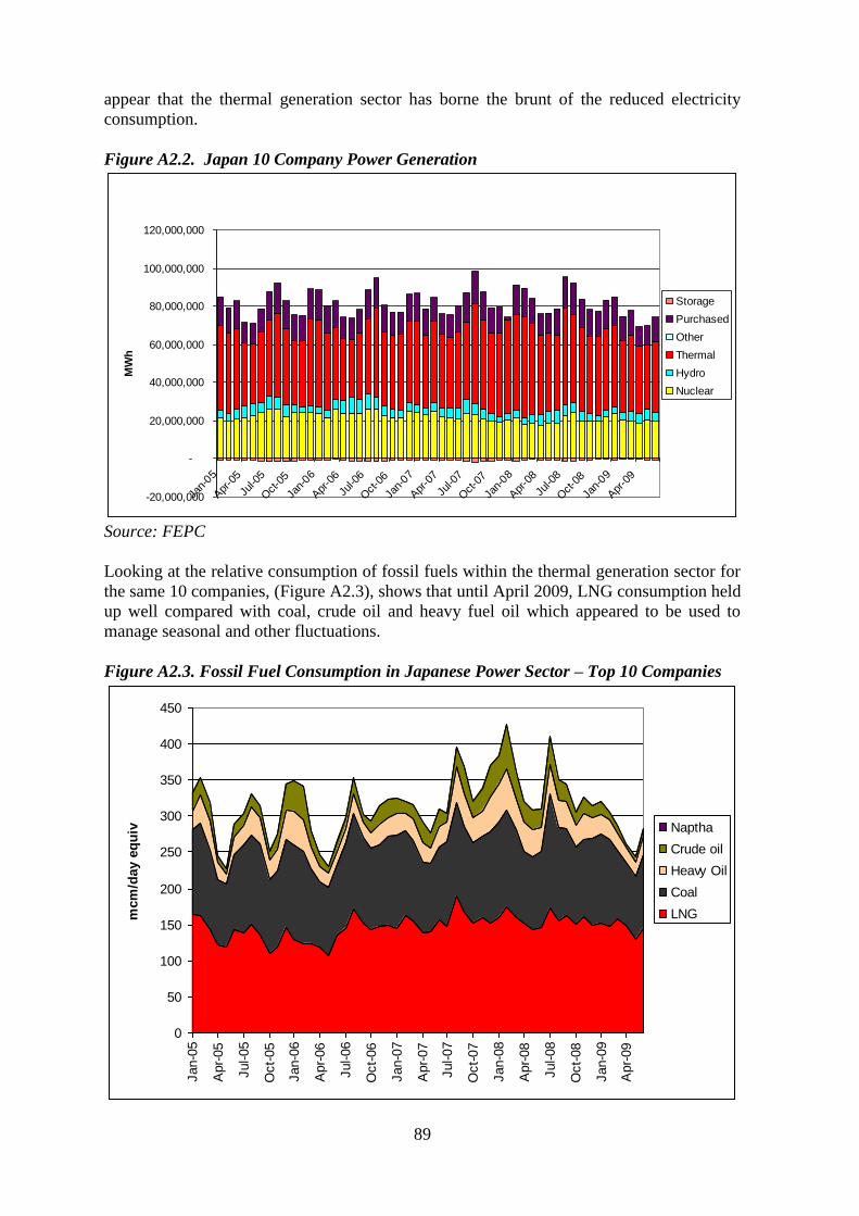
89
appear that the thermal generation sector has borne the brunt of the reduced electricity
consumption.
Figure A2.2. Japan 10 Company Power Generation
-20,000,000
-
20,000,000
40,000,000
60,000,000
80,000,000
100,000,000
120,000,000
Jan-
05
Apr
-05
Jul-0
5
Oct-0
5
Jan-
06
Apr
-06
Jul-0
6
Oct-0
6
Jan-
07
Apr
-07
Jul-0
7
Oct-0
7
Jan-
08
Apr
-08
Jul-0
8
Oct-0
8
Jan-
09
Apr
-09
MW
h
Storage
Purchased
Other
Thermal
Hydro
Nuclear
Source: FEPC
Looking at the relative consumption of fossil fuels within the thermal generation sector for
the same 10 companies, (Figure A2.3), shows that until April 2009, LNG consumption held
up well compared with coal, crude oil and heavy fuel oil which appeared to be used to
manage seasonal and other fluctuations.
Figure A2.3. Fossil Fuel Consumption in Japanese Power Sector – Top 10 Companies
0
50
100
150
200
250
300
350
400
450
Jan-0
5
Apr-
05
Jul-05
Oct-
05
Jan-0
6
Apr-
06
Jul-06
Oct-
06
Jan-0
7
Apr-
07
Jul-07
Oct-
07
Jan-0
8
Apr-
08
Jul-08
Oct-
08
Jan-0
9
Apr-
09
mcm
/day e
qu
iv Naptha
Crude oil
Heavy Oil
Coal
LNG

90
Source: FEPC
Figure A2.4. Japan Natural Gas Supply and Demand 2000 – 2008
0
20
40
60
80
100
120
2000 2001 2002 2003 2004 2005 2006 2007 2008
bc
ma
LNG Imports
Production
Demand
Source: BP 2009, IEA Monthly Data Series
Figure A2.4 shows the total Japanese natural gas annual supply and demand position and
clearly shows the increase in demand in 2007-08. Whether such increased consumption
will continue once Japan‟s nuclear sector recovers to more typical historic output levels is
now a moot point as the economic recession has overtaken these considerations and has
depressed demand overall.
Figure A2.5. Japanese LNG Imports 2004 - 2009
0
50
100
150
200
250
300
jan feb mar apr may jun jul aug sep oct nov dec
mcm
/day 2006
2007
2008
2009
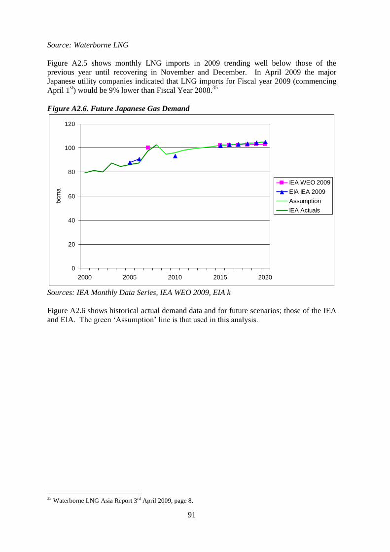
91
Source: Waterborne LNG
Figure A2.5 shows monthly LNG imports in 2009 trending well below those of the
previous year until recovering in November and December. In April 2009 the major
Japanese utility companies indicated that LNG imports for Fiscal year 2009 (commencing
April 1st) would be 9% lower than Fiscal Year 2008.
35
Figure A2.6. Future Japanese Gas Demand
0
20
40
60
80
100
120
2000 2005 2010 2015 2020
bcm
a
IEA WEO 2009
EIA IEA 2009
Assumption
IEA Actuals
Sources: IEA Monthly Data Series, IEA WEO 2009, EIA k
Figure A2.6 shows historical actual demand data and for future scenarios; those of the IEA
and EIA. The green „Assumption‟ line is that used in this analysis.
35
Waterborne LNG Asia Report 3rd
April 2009, page 8.

92
South Korea
Figure A2.7. South Korea Primary Energy Consumption 2000 – 2008
0
50
100
150
200
250
300
2000 2001 2002 2003 2004 2005 2006 2007 2008
Mil
lio
n T
on
nes O
il E
qu
ivale
nt
0%
5%
10%
15%
20%
25%
30%
Hydro
Nuclear
Natural Gas
Coal
Oil & Oil Products
Natural Gas %
Source: BP 2009
Figure A2.7 shows South Korean primary energy consumption on a steady growth trend to
2008 with Natural Gas and Coal accounting for most of the increase. Over the period gas‟
share of primary energy grew from 10% to 15%.
Figure A2.8. South Korea Electricity Generation
0
50
100
150
200
250
300
350
400
450
500
2000 2001 2002 2003 2004 2005 2006 2007 2008
TW
h
Source: BP 2009

93
While comprehensive data on Korean power sector fuel usage is not readily available,
Figure A2.8 shows a strong consistent growth trend of 4 – 5% pa.
Figure A2.9. South Korea Natural Gas Supply & Demand
0
5
10
15
20
25
30
35
40
45
2000 2001 2002 2003 2004 2005 2006 2007 2008
bc
ma
LNG
Prodn
Demand
Sources: BP 2009, Waterborne LNG, IEA Monthly Data Series
Figure A2.9 shows South Korea‟s natural gas supply and demand position from 2000 to
2008. Apart from very minor domestic production beginning in 2007, South Korea relies
on LNG for all its natural gas supply. The picture here is one of steady growth however, as
with Japan, the impact of the 2009 economic recession has changed this post 2008.
Figure A2.10. South Korea Monthly LNG Imports
0
20
40
60
80
100
120
140
160
180
jan feb mar apr may jun jul aug sep oct nov dec
mm
cm
/day 2006
2007
2008
2009
Source: Waterborne LNG

94
In the first half of 2009 LNG imports were down 12% compared with the previous year
(Figure A2.10). In the final quarter of 2009 however, demand had recovered to the levels
observed in 2008.
Figure A2.11. South Korea Future Gas Demand
0
5
10
15
20
25
30
35
40
45
50
2000 2005 2010 2015 2020
bcm
a
IEA Actuals
A Flow er Base Case
EIA IEA 2009
Sources: IEA Monthly Data Series, EIAk, Flower 2009c
Figure A2.11 shows historical actual demand data and future scenarios from the EIA and
Andy Flower. Andy Flower‟s „Base Case‟ scenario for future demand is used in this
analysis.

95
Taiwan
Figure A2.12. Taiwan Primary Energy Consumption
-10
10
30
50
70
90
110
130
150
2000 2001 2002 2003 2004 2005 2006 2007 2008
Mil
lio
n T
on
nes O
il E
qu
ivale
nt
0%
5%
10%
15%
20%
25%
30%
Hydro
Nuclear
Natural Gas
Coal
Oil & Oil Products
Natural Gas %
Source: BP 2009
While its primary energy consumption is about half of that of South Korea, Taiwan has a
broadly similar pattern of fuel usage. From 2003 to 2007 gas and coal were the fuels
showing the greatest consumption growth (Figure A2.12). By 2008 natural gas still
accounted for only 10% of primary energy consumption.
Figure A2.13. Taiwan Electricity Generation
0
50
100
150
200
250
300
2000 2001 2002 2003 2004 2005 2006 2007 2008
TW
h
Source: BP 2009

96
The steady growth in power generation seen in the early part of the decade faded somewhat
in 2008 in line with a similar pattern in primary energy consumption (Figure A2.13).
Figure A2.14. Taiwan Natural Gas Supply & Demand
0
2
4
6
8
10
12
14
2000 2001 2002 2003 2004 2005 2006 2007 2008
bcm
a LNG
Prodn
Demand
Sources: BP 2009, EIAj
Figure A2.14 shows the Taiwanese natural gas supply and demand position from 2000 to
2008. With domestic supply waning, Taiwan‟s demand growth is overwhelmingly met by
LNG imports.
Figure A2.15. Taiwan Monthly LNG Imports
0
5
10
15
20
25
30
35
40
45
50
jan feb mar apr may jun jul aug sep oct nov dec
mcm
/day 2006
2007
2008
2009
Source: Waterborne LNG
Taiwan has a summer peak demand load which is reflected in the pattern of LNG imports
shown in Figure A2.15. Of note is the 13% reduction in imports in the first half of 2009
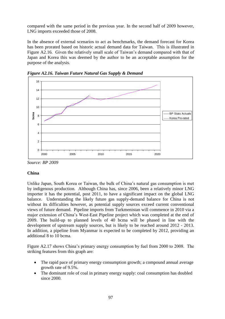
97
compared with the same period in the previous year. In the second half of 2009 however,
LNG imports exceeded those of 2008.
In the absence of external scenarios to act as benchmarks, the demand forecast for Korea
has been prorated based on historic actual demand data for Taiwan. This is illustrated in
Figure A2.16. Given the relatively small scale of Taiwan‟s demand compared with that of
Japan and Korea this was deemed by the author to be an acceptable assumption for the
purpose of the analysis.
Figure A2.16. Taiwan Future Natural Gas Supply & Demand
0
2
4
6
8
10
12
14
16
2000 2005 2010 2015 2020
bcm
a BP Stats Actuals
Korea Pro-rated
Source: BP 2009
China
Unlike Japan, South Korea or Taiwan, the bulk of China‟s natural gas consumption is met
by indigenous production. Although China has, since 2006, been a relatively minor LNG
importer it has the potential, post 2011, to have a significant impact on the global LNG
balance. Understanding the likely future gas supply-demand balance for China is not
without its difficulties however, as potential supply sources exceed current conventional
views of future demand. Pipeline imports from Turkmenistan will commence in 2010 via a
major extension of China‟s West-East Pipeline project which was completed at the end of
2009. The build-up to planned levels of 40 bcma will be phased in line with the
development of upstream supply sources, but is likely to be reached around 2012 - 2013.
In addition, a pipeline from Myanmar is expected to be completed by 2012, providing an
additional 8 to 10 bcma.
Figure A2.17 shows China‟s primary energy consumption by fuel from 2000 to 2008. The
striking features from this graph are:
The rapid pace of primary energy consumption growth; a compound annual average
growth rate of 9.5%.
The dominant role of coal in primary energy supply: coal consumption has doubled
since 2000.

98
The very small (but growing) share of gas in primary energy consumption; growing
from 2.5% to 3.7% in the period shown.
Figure A2.17. China Primary Energy Consumption 2000 – 2008
0
500
1000
1500
2000
2500
2000 2001 2002 2003 2004 2005 2006 2007 2008
Mil
lio
n T
on
ne
s O
il E
qu
iva
len
t
0.0%
0.5%
1.0%
1.5%
2.0%
2.5%
3.0%
3.5%
4.0%
4.5%
5.0%
Hydro
Nuclear
Natural Gas
Coal
Oil & Oil Products
Natural Gas %
Source: BP 2009
Figure A2.18. China Natural Gas Demand 2006 - 2020
0
20
40
60
80
100
120
140
160
180
200
2006 2007 2008 2009 2010 2011 2012 2013 2014 2015 2016 2017 2018 2019 2020
bcm
a
EIA
IEA
IHS (2005)
BP Stats
Sources: IEA WEO2009, EIAk, IHS 2005, slide 19, BP 2009

99
The challenges posed in deriving credible future assumptions for Chinese LNG import
requirement are therefore:
The difficulties of predicting gas consumption growth given its small but growing
share of a rapidly growing primary energy base in China.
Predicting the supply mix (domestic production, pipeline imports and LNG) given
uncertainties in all these components.
Figure A2.18 shows three scenarios for natural gas demand in China and actual data for
2006 – 2008. The IEA scenario is most in line with recent data and this has been used as a
starting point.
Figure A2.19 shows views of domestic natural gas production from the same sources.
Figure A2.19. China Domestic Natural Gas Production 2006 - 2020
0
20
40
60
80
100
120
140
2006 2007 2008 2009 2010 2011 2012 2013 2014 2015 2016 2017 2018 2019 2020
bcm
a
EIA
IHS (2005)
Base Case
BP Stats
IEA
Sources: WEO2009, EIAj, IHS 2005, slide 19, BP 2009
Clearly there is a wide range of uncertainty. The dashed purple line is the assumption used
in this analysis.
Figure A2.20. China Natural Gas Supply and Demand – Initial View
0
20
40
60
80
100
120
140
160
180
200
2006 2007 2008 2009 2010 2011 2012 2013 2014 2015 2016 2017 2018 2019 2020
bcm
a
LNG
Pipeline - Myanmar
Pipeline - China
Production
Demand
Sources: Author’s analysis.
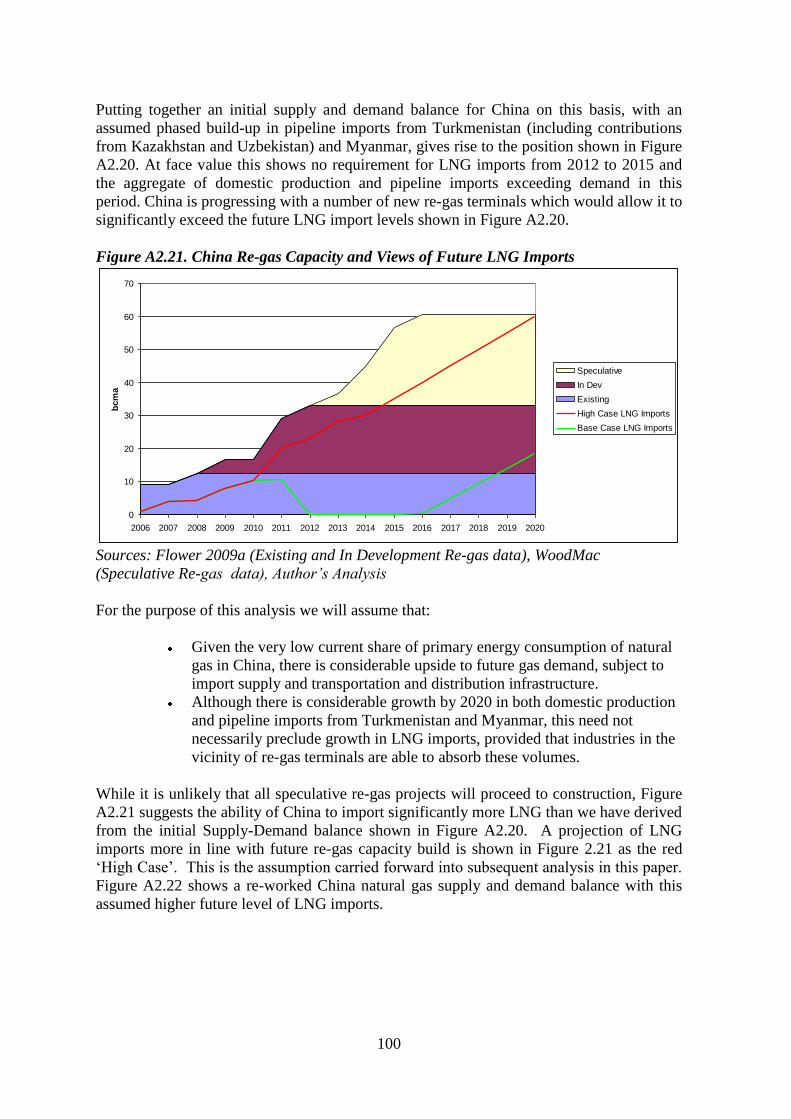
100
Putting together an initial supply and demand balance for China on this basis, with an
assumed phased build-up in pipeline imports from Turkmenistan (including contributions
from Kazakhstan and Uzbekistan) and Myanmar, gives rise to the position shown in Figure
A2.20. At face value this shows no requirement for LNG imports from 2012 to 2015 and
the aggregate of domestic production and pipeline imports exceeding demand in this
period. China is progressing with a number of new re-gas terminals which would allow it to
significantly exceed the future LNG import levels shown in Figure A2.20.
Figure A2.21. China Re-gas Capacity and Views of Future LNG Imports
0
10
20
30
40
50
60
70
2006 2007 2008 2009 2010 2011 2012 2013 2014 2015 2016 2017 2018 2019 2020
bcm
a
Speculative
In Dev
Existing
High Case LNG Imports
Base Case LNG Imports
Sources: Flower 2009a (Existing and In Development Re-gas data), WoodMac
(Speculative Re-gas data), Author’s Analysis
For the purpose of this analysis we will assume that:
Given the very low current share of primary energy consumption of natural
gas in China, there is considerable upside to future gas demand, subject to
import supply and transportation and distribution infrastructure.
Although there is considerable growth by 2020 in both domestic production
and pipeline imports from Turkmenistan and Myanmar, this need not
necessarily preclude growth in LNG imports, provided that industries in the
vicinity of re-gas terminals are able to absorb these volumes.
While it is unlikely that all speculative re-gas projects will proceed to construction, Figure
A2.21 suggests the ability of China to import significantly more LNG than we have derived
from the initial Supply-Demand balance shown in Figure A2.20. A projection of LNG
imports more in line with future re-gas capacity build is shown in Figure 2.21 as the red
„High Case‟. This is the assumption carried forward into subsequent analysis in this paper.
Figure A2.22 shows a re-worked China natural gas supply and demand balance with this
assumed higher future level of LNG imports.
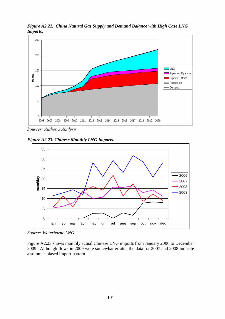
101
Figure A2.22. China Natural Gas Supply and Demand Balance with High Case LNG
Imports.
0
50
100
150
200
250
2006 2007 2008 2009 2010 2011 2012 2013 2014 2015 2016 2017 2018 2019 2020
bcm
a
LNG
Pipeline - Myanmar
Pipeline - China
Production
Demand
Sources: Author’s Analysis
Figure A2.23. Chinese Monthly LNG Imports.
0
5
10
15
20
25
30
35
jan feb mar apr may jun jul aug sep oct nov dec
mc
m/d
ay 2006
2007
2008
2009
Source: Waterborne LNG
Figure A2.23 shows monthly actual Chinese LNG imports from January 2006 to December
2009. Although flows in 2009 were somewhat erratic, the data for 2007 and 2008 indicate
a summer-biased import pattern.

102
India
Figure A2.24 shows very clearly the dominance of coal in India‟s primary energy make-up
from 2000 to 2008. In this period primary energy consumption grew at an annual average
rate of 5.9%. Natural gas‟ share held at around 11 to 12 % through the period.
Figure A2.24. India Primary Energy Consumption 2000 - 2008
0
50
100
150
200
250
300
350
400
2000 2001 2002 2003 2004 2005 2006 2007 2008
Mil
lio
n T
on
ne
s O
il q
uiv
ale
nt
0.0%
2.0%
4.0%
6.0%
8.0%
10.0%
12.0%
14.0%
16.0%
18.0%
20.0%
Hydro
Nuclear
Natural Gas
Coal
Oil & Oil Products
Natural Gas %
Source: BP 2009
Figure A2.25. India Gas Supply & Demand 2000 - 2008
0
5
10
15
20
25
30
35
40
45
2000 2001 2002 2003 2004 2005 2006 2007 2008
bc
ma LNG Imports
Production
Demand
Source: BP 2009

103
India‟s natural gas position is shown in Figure A2.25. Demand grew by 5.8% per annum
through the period. 2004 saw the start of LNG imports as demand outstripped domestic
supply.
As with China, gas‟ relatively low share of primary energy, combined with a high growth
economy in the context of the 2009 economic recession, make forecasting future demand
challenging.
Figure A2.26 shows three demand scenarios for India‟s natural gas demand to 2020.
Figure A2.26. India Natural Gas Demand 2006 - 2020
0
20
40
60
80
100
120
140
2006 2007 2008 2009 2010 2011 2012 2013 2014 2015 2016 2017 2018 2019 2020
bcm
a
EIA
IEA
IHS (2005)
BP Stats
Sources: IEA WEO2009, EIAk, IHS 2005, slide 19, BP 2009
The IHS view (made in 2005) is much higher than those of the IEA and EIA, between
which there is convergence by 2020. For this analysis the IEA WEO2009 scenario was
used as an initial basis.
Figure A2.27. India Domestic Natural Gas Production 2006 - 2020
0
10
20
30
40
50
60
70
2006 2007 2008 2009 2010 2011 2012 2013 2014 2015 2016 2017 2018 2019 2020
bcm
a
EIA
IHS (2005)
BP Stats
Base Case
IEA
Sources: WEO2009, EIAj, IHS 2005, slide 19, BP 2009
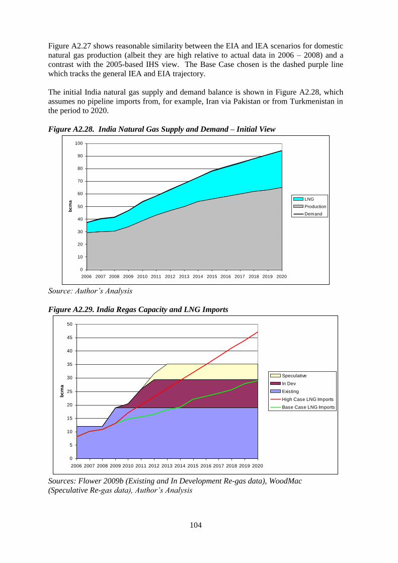
104
Figure A2.27 shows reasonable similarity between the EIA and IEA scenarios for domestic
natural gas production (albeit they are high relative to actual data in 2006 – 2008) and a
contrast with the 2005-based IHS view. The Base Case chosen is the dashed purple line
which tracks the general IEA and EIA trajectory.
The initial India natural gas supply and demand balance is shown in Figure A2.28, which
assumes no pipeline imports from, for example, Iran via Pakistan or from Turkmenistan in
the period to 2020.
Figure A2.28. India Natural Gas Supply and Demand – Initial View
0
10
20
30
40
50
60
70
80
90
100
2006 2007 2008 2009 2010 2011 2012 2013 2014 2015 2016 2017 2018 2019 2020
bc
ma
LNG
Production
Demand
Source: Author’s Analysis
Figure A2.29. India Regas Capacity and LNG Imports
0
5
10
15
20
25
30
35
40
45
50
2006 2007 2008 2009 2010 2011 2012 2013 2014 2015 2016 2017 2018 2019 2020
bc
ma
Speculative
In Dev
Existing
High Case LNG Imports
Base Case LNG Imports
Sources: Flower 2009b (Existing and In Development Re-gas data), WoodMac
(Speculative Re-gas data), Author’s Analysis

105
As with China, India is progressing new re-gas projects which will increase its import
capacity for LNG from 2011. The growth in re-gas capacity is shown in Figure A2.29
together with an initial „base case‟ view of LNG imports and a potentially higher LNG
import case.
We will use the High Case LNG Import assumptions in subsequent analysis. For
completeness the Indian future natural gas supply & demand position is re-constructed in
Figure A2.30 with the higher LNG import assumption and consequently higher demand.
Figure A2.30. India Natural Gas Supply and Demand Balance with High Case LNG
Imports.
0
20
40
60
80
100
120
2006 2007 2008 2009 2010 2011 2012 2013 2014 2015 2016 2017 2018 2019 2020
bc
ma
LNG
Production
Demand
Source: Author’s Analysis
Figure A2.31 shows the aggregate LNG import requirement for the existing Asian LNG
markets to 2020, and the impact of India and China‟s growing LNG requirement.
Figure A2.31. Asian LNG Import Forecast
0
50
100
150
200
250
300
2005 2010 2015 2020
bcm
a
China
India
Taiwan
South Korea
Japan
Source: Author’s Analysis

106
Europe
Europe, for the purposes of this model framework, includes:
Austria, Belgium, Bulgaria, Croatia, Czech Republic, Denmark, Estonia, Finland, France,
Germany, Greece, Hungary, Ireland, Italy, Latvia, Lithuania Luxembourg, Netherlands,
Norway, Poland, Portugal, Romania, Serbia, Slovakia, Slovenia, Spain, Sweden,
Switzerland, Turkey, UK.
Demand
Figure A2.32 represents a „consensus‟ view of European natural gas demand prior to the
onset of the 2008 / 2009 economic recession. It is broadly consistent with the IEA WEO
2008 for comparable geographies. Overall growth from 2008 to 2020 is 1.4% CAGR36
,
with growth of 0.4% pa in the Industrial sector, 1.0% in the Residential and Commercial
sector and 2.4% in the power generation sector.
Figure A2.32. European Demand – Pre-Recession View
0
100
200
300
400
500
600
700
800
2000 2005 2010 2015 2020
bcm
a Power
Res& Com
Industry
Source: IEA Annual Data Series, IEA WEO 2008, Author’s Analysis
From 4Q 2008 onwards it became apparent that natural gas consumption was falling short
of levels expected for the prevailing temperatures37
. This is illustrated in Figure A2.33.
36
CAGR = Compound Average Annual Growth Rate. 37
Weather Underground

107
Figure A2.33. European Demand January 2008 – October 2009
0
500
1000
1500
2000
2500
3000
Ja
n-0
8
Fe
b-0
8
Ma
r-0
8
Ap
r-0
8
Ma
y-0
8
Ju
n-0
8
Ju
l-0
8
Au
g-0
8
Se
p-0
8
Oct-
08
No
v-0
8
De
c-0
8
Ja
n-0
9
Fe
b-0
9
Ma
r-0
9
Ap
r-0
9
Ma
y-0
9
Ju
n-0
9
Ju
l-0
9
Au
g-0
9
Se
p-0
9
Oct-
09
mc
m/d
ay
Normal Year
Actual
Predicted given Temps
Source: IEA Monthly Data Series, Author’s Analysis
Based on a correlation between average monthly temperature and demand for the major gas
consuming countries of Europe, Figure A2.33 shows:
Demand already beginning to undershoot expected levels for the prevailing
temperatures in Spring 2008 – potentially caused by space heating efficiency
measures in response to price.
A growing and sustained divergence between actual demand and demand expected
at the prevailing temperatures from 4Q08 onwards.
Some apparent narrowing of the „actual vs. predicted‟ gap in 3Q 2009, possibly due
to increased industrial sector demand as the recession-related inventory run-down
cycle ended.
Actual gas demand in the period Jan 2009 to October 2009 was 8.5% lower than the same
period in 2008 and 14% lower than what would be expected at the prevailing temperatures.
In constructing our future demand assumption envelope for Europe the major uncertainty is
the demand recovery trajectory post – recession. Figure A2.34 shows actual European
demand to 2008 and future scenarios from the IEA, EIA and ExxonMobil. The EIA
scenario does not appear to have incorporated recessionary demand destruction and the
IEA does not provide annual data points for the period between 2009 and 2015. A working
assumption was derived by taking a trajectory in between the IEA WEO2009 scenario and
the ExxonMobil scenario, which is shown as the light green line in Figure A2.34.
Given the prevailing uncertainty on the timing and pace of gas demand growth as Europe
emerges from recession, the author has not re-appraised the future sectoral demand
analysis. (see Honore, Forthcoming 2010)

108
Figure A2.34. European Demand Assumptions
0
100
200
300
400
500
600
700
800
2000 2005 2010 2015 2020
bcm
a
IEA Actuals
ExxonMobil 2010
IEA WEO2009
EIA IEA 2009
Assumption
Source: ExxonMobil 2009 p.29, IEA WEO2009, IEA Monthly Data Series, EIAk
The other aspect of demand to consider is the seasonal monthly demand variation. In the
modelling framework, historical monthly demand profiles are combined with future annual
demand to produce a monthly forecast at a country level which is then aggregated to a
European region total.
Domestic Production
Figure A2.35. European Natural Gas Production
0
50
100
150
200
250
300
350
400
2000 2005 2010 2015 2020
bcm
a
Norway
Others
Italy
Romania
Denmark
Netherlands
Germany
UK
Sources: IEA Monthly Data Series, National Grid, NPD, OGP, Author’s Analysis

109
Historical actual production is taken from the IEA Monthly Data Series and key estimates
of future production levels from:
The Norwegian Petroleum Directorate to benchmark future Norwegian
Production.
The International Association of Oil and Gas Producers, for Netherlands
Production
National Grid to benchmark UK production future decline.
Future production levels for other European producing countries were calculated by
extrapolation of existing trends.
Figure A2.35 shows actual European domestic production from 2000 and the assumed
trend to 2020. The figure shows decline at varying rates in all countries except Norway.
Norway is able to offset decline elsewhere in Europe until 2010. Beyond 2010 the
aggregate European production trend is one of decline.
During 2009 and in 2010, given the success of unconventional gas production in the US
and Canada, there has been considerable interest in Europe‟s unconventional gas
production potential. At this stage however, there is uncertainty as to the scale and timing
of future European unconventional gas production. The IEA WEO 2009 envisaged only
some 15 bcma of unconventional gas production in Europe, post 202038
.
Figure A2.36. European Domestic Production – Monthly Basis
0
200
400
600
800
1000
1200
Jan-0
5
Jan-0
6
Jan-0
7
Jan-0
8
Jan-0
9
Jan-1
0
Jan-1
1
Jan-1
2
Jan-1
3
Jan-1
4
Jan-1
5
Jan-1
6
Jan-1
7
Jan-1
8
Jan-1
9
Jan-2
0
mcm
/day
Source: IEA Monthly Data Series, Author’s Analysis
Figure A2.36 shows historic actual data to early 2009 and the future projection obtained by
applying an average monthly profile to future annual production forecasts at a country
level. In addition to the decline in absolute production the summer – winter flexibility is
also reduced.
38
IEA WEO 2009, p. 478
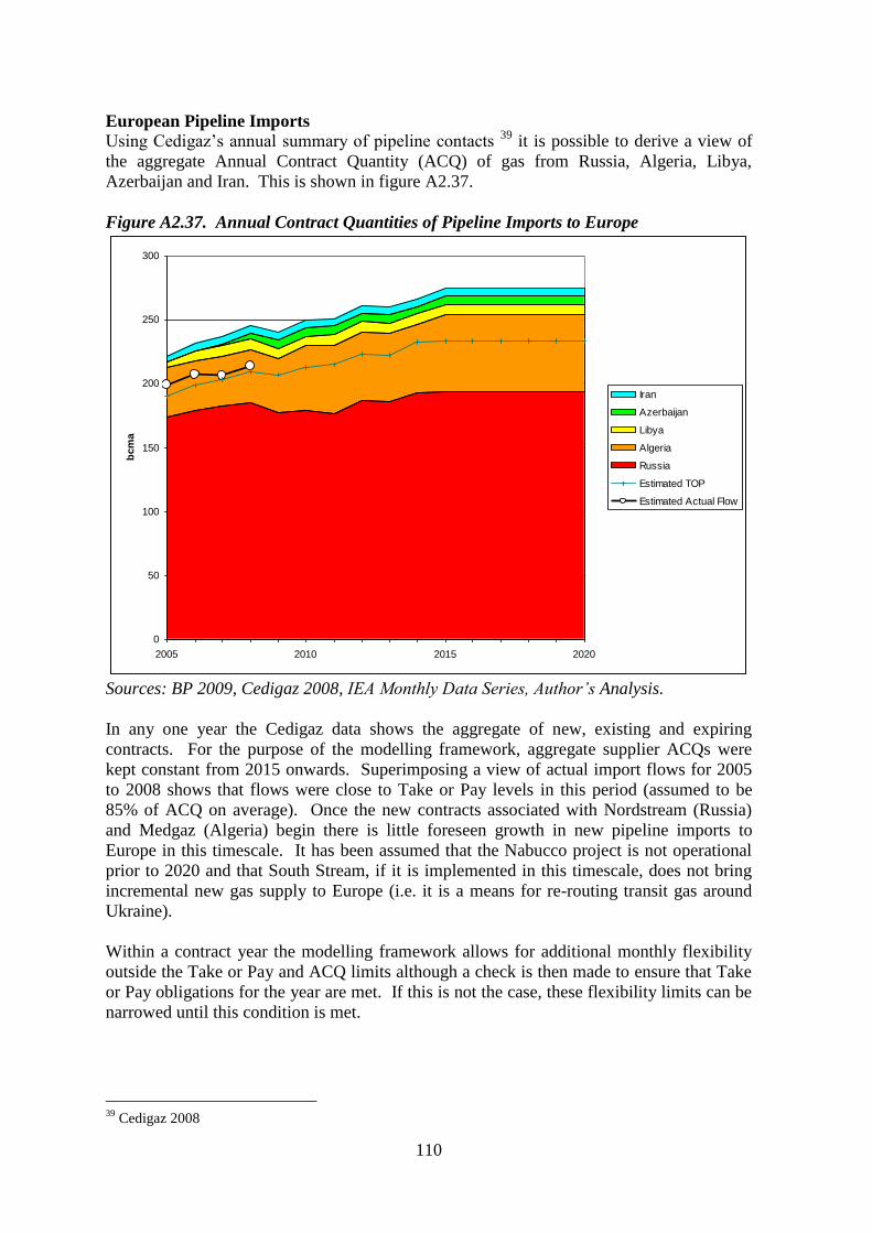
110
European Pipeline Imports
Using Cedigaz‟s annual summary of pipeline contacts 39
it is possible to derive a view of
the aggregate Annual Contract Quantity (ACQ) of gas from Russia, Algeria, Libya,
Azerbaijan and Iran. This is shown in figure A2.37.
Figure A2.37. Annual Contract Quantities of Pipeline Imports to Europe
0
50
100
150
200
250
300
2005 2010 2015 2020
bcm
a
Iran
Azerbaijan
Libya
Algeria
Russia
Estimated TOP
Estimated Actual Flow
Sources: BP 2009, Cedigaz 2008, IEA Monthly Data Series, Author’s Analysis.
In any one year the Cedigaz data shows the aggregate of new, existing and expiring
contracts. For the purpose of the modelling framework, aggregate supplier ACQs were
kept constant from 2015 onwards. Superimposing a view of actual import flows for 2005
to 2008 shows that flows were close to Take or Pay levels in this period (assumed to be
85% of ACQ on average). Once the new contracts associated with Nordstream (Russia)
and Medgaz (Algeria) begin there is little foreseen growth in new pipeline imports to
Europe in this timescale. It has been assumed that the Nabucco project is not operational
prior to 2020 and that South Stream, if it is implemented in this timescale, does not bring
incremental new gas supply to Europe (i.e. it is a means for re-routing transit gas around
Ukraine).
Within a contract year the modelling framework allows for additional monthly flexibility
outside the Take or Pay and ACQ limits although a check is then made to ensure that Take
or Pay obligations for the year are met. If this is not the case, these flexibility limits can be
narrowed until this condition is met.
39
Cedigaz 2008

111
LNG
Combining the assumptions for future European demand, pipeline imports at take or pay
contract levels and domestic gas production allows us to take a view of maximum LNG
requirements. These are shown in Figure A2.38, growing to reach some 190 bcma by
2020.
Figure A2.38. Sources of European Supply.
0
100
200
300
400
500
600
700
2005 2010 2015 2020
bcm
a
Domestic Production Actual Pipeline Imports Future Pipeline TOP
Maximum LNG Requirement Demand
Source: BP2009, Author’s Analysis
As a sense check, Figure A2.39 compares these annual LNG import volumes (blue line)
with a view of European re-gas capacity in „existing‟, „in development‟ and „speculative‟
categories. In aggregate, Europe has sufficient re-gas capacity either existing or in
development to meet the 2020 import requirement. Where additional capacity is required
there is more than sufficient lead time to construct this.
Figure A2.39. European Maximum LNG Import Requirement and Regas Capacity
0
50
100
150
200
250
300
350
400
450
2005 2010 2015 2020
bc
ma
Regas Existing Regas In Development Regas Speculative LNG Imports
Sources: WoodMac 2008a, Author’s Analysis

112
Gas Storage
The model framework uses European storage to provide part of the supply flexibility to
meet seasonal demand variation. Due to the nature of the modelling approach seasonal
storage is handled as follows:
Historic actuals are derived from a combination of IEA Monthly Data and Gas
Storage Europe (GSE) data.40
A future storage new-build rate of around 2.5 bcm per year of working gas capacity
is assumed.
A typical annual injection-withdrawal profile has been derived from historic data.
Combining this with the projected working gas capacity allows the future path of
total European storage inventory to be projected assuming an „average‟ year in
terms of weather – related demand.
Great care must be taken in transitioning from the most recent actual data into the
„generated‟ future inventory forecast in order to avoid large anomalous inventory
movements in the transition zone.
North America
The future assumptions used in the modelling framework are described below for the US,
Canada and Mexico demand and domestic production.
US Demand
Despite its size and relative maturity there has for some while been a lack of consensus
between market observers as to the future growth in US natural gas demand. Industrial
demand has been on a 10 year downward trend and the residential and commercial sector is
arguably saturated. Power generation has been the most dynamic sector in terms of
consumption growth, however around 50% of power generation continues to be coal-fired.
The most optimistic forecasters generally assumed further growth in gas fired generation
given the relatively low number of new coal fired plant under construction or planned. The
more pessimistic observers may well have shied away from high gas demand growth
forecasts, because of the implication that additional LNG imports would be needed (before
the potential for unconventional gas exploitation at scale became apparent).
The economic recession has had only a muted impact on gas demand in Canada and the
USA. This is shown in Figure A2.40. For the period January 2009 to October 2009, gas
demand was 2.1% lower than the same months of 2008. The EIA in its monthly Short
Term Energy Outlooks has commented that the fall in industrial sector gas demand in the
USA has been offset by increased consumption in the power generation sector.
40
Note that the IEA data includes all national inventory including line pack. The author believes that this
figure is calculated by deriving stock changes month-on-month and therefore cumulative errors may well
have crept in over time. The GSE data although recently much improved in terms of coverage, lacks
historical continuity. Judgement must be applied in arriving at a view of end month „actual‟ storage inventory.

113
Figure A2.40. USA and Canada Gas Demand 2008 and 2009.
-
500
1,000
1,500
2,000
2,500
3,000
3,500
Jan Feb Mar Apr May Jun Jul Aug Sep Oct Nov Dec
mc
m/d
ay
2008
2009
Source: EIAb
Figure A2.41. Range of Views of Future US Natural Gas Demand
0
100
200
300
400
500
600
700
800
2000 2005 2010 2015 2020
bcm
a
ExxonMobil 2009
IEA WEO 2009
EIA AEO 2010
Assumption
EIA Historic Actuals
Sources: EIAl , ExxonMobil 2009 p 29, IEA WEO2009
Figure A2.41 shows historical annual US gas demand data from 2000 to 2008 and future
demand scenarios from ExxonMobil, the EIA and the IEA. These views vary significantly
with ExxonMobil anticipating growth post 2015 and the EIA anticipating a decline in gas
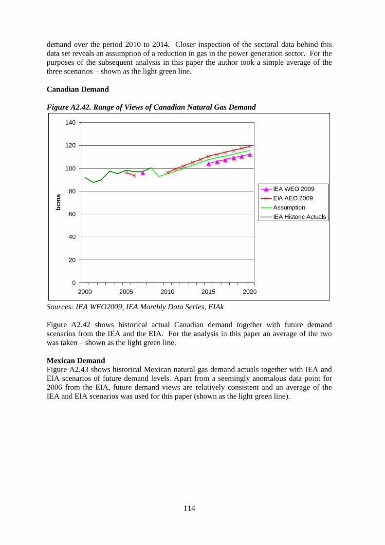
114
demand over the period 2010 to 2014. Closer inspection of the sectoral data behind this
data set reveals an assumption of a reduction in gas in the power generation sector. For the
purposes of the subsequent analysis in this paper the author took a simple average of the
three scenarios – shown as the light green line.
Canadian Demand
Figure A2.42. Range of Views of Canadian Natural Gas Demand
0
20
40
60
80
100
120
140
2000 2005 2010 2015 2020
bc
ma
IEA WEO 2009
EIA AEO 2009
Assumption
IEA Historic Actuals
Sources: IEA WEO2009, IEA Monthly Data Series, EIAk
Figure A2.42 shows historical actual Canadian demand together with future demand
scenarios from the IEA and the EIA. For the analysis in this paper an average of the two
was taken – shown as the light green line.
Mexican Demand
Figure A2.43 shows historical Mexican natural gas demand actuals together with IEA and
EIA scenarios of future demand levels. Apart from a seemingly anomalous data point for
2006 from the EIA, future demand views are relatively consistent and an average of the
IEA and EIA scenarios was used for this paper (shown as the light green line).

115
Figure A2.43. Mexican Natural Gas Demand Scenarios
0
10
20
30
40
50
60
70
80
90
100
2000 2005 2010 2015 2020
bcm
a
IEA Historic Actuals
IEA Weo 2009
EIA AEO 2009
Assumption
Sources: IEA Monthly Data Series, IEA WEO2009, EIAk.
North American Production
In Chapter 1 we noted the post 2005 turn-around in the prospects for US production due to
the successful exploitation of „unconventional‟ gas - coal bed methane and especially shale
gas. Industry commentary in 2008 alluded to shale gas „plays‟ needing of the order of $6
to $8/mmbtu gas price to support economic development. More recently in 2009, the
figures quoted vary and some estimates are lower. Figure 2.44 shows the drastic reduction
in gas-focussed drilling activity in the US since spot gas prices declined.
Figure A2.44. US Gas Rig Count and Henry Hub Price
0
200
400
600
800
1000
1200
1400
1600
1800
Jan-
08
Feb-0
8
Mar
-08
Apr
-08
May
-08
Jun-
08
Jul-0
8
Aug
-08
Sep
-08
Oct-0
8
Nov-
08
Dec-
08
Jan-
09
Feb-0
9
Mar
-09
Apr
-09
May
-09
Jun-
09
Jul-0
9
Aug
-09
Sep
-09
Oct-0
9
Nov-
09
Dec-
09
Gas R
ig C
ou
nt
0
2
4
6
8
10
12
14
16
18
Hen
ry H
ub
Pri
ce $
/mm
btu
US Gas Rig Count Henry Hub
Sources: Argus, Baker Hughes 2009

116
Despite the reduction in gas rig count (by July 2009 it was 43% of the September 2008
level), up to October 2009, the impact on US dry gas production levels appears to be muted
(Figure A2.45).
Figure A2.45. US Gas Rig Count and US Dry Gas Production
0
200
400
600
800
1000
1200
1400
1600
1800
2000
Ja
n-0
8
Feb
-08
Ma
r-0
8
Ap
r-08
Ma
y-0
8
Ju
n-0
8
Ju
l-08
Au
g-0
8
Se
p-0
8
Oct-
08
No
v-0
8
De
c-0
8
Ja
n-0
9
Feb
-09
Ma
r-0
9
Ap
r-09
Ma
y-0
9
Ju
n-0
9
Ju
l-09
Au
g-0
9
Se
p-0
9
Oct-
09
No
v-0
9
De
c-0
9
Rig
Co
un
t o
r G
as
Pro
du
cti
on
mc
m/d
ay
US Gas Rig Count US Dry Gas Production
Sources: EIAb, Baker Hughes 2009
Note that the dip in production in September and October 2008 was a consequence of
Hurricane Gustav. Although gas production shows a minor reduction from around March
2009, this is not proportional to the rig count reduction, implying a significant lagged
response or alternatively that US drilling activity is concentrating on higher productivity
gas prospects.
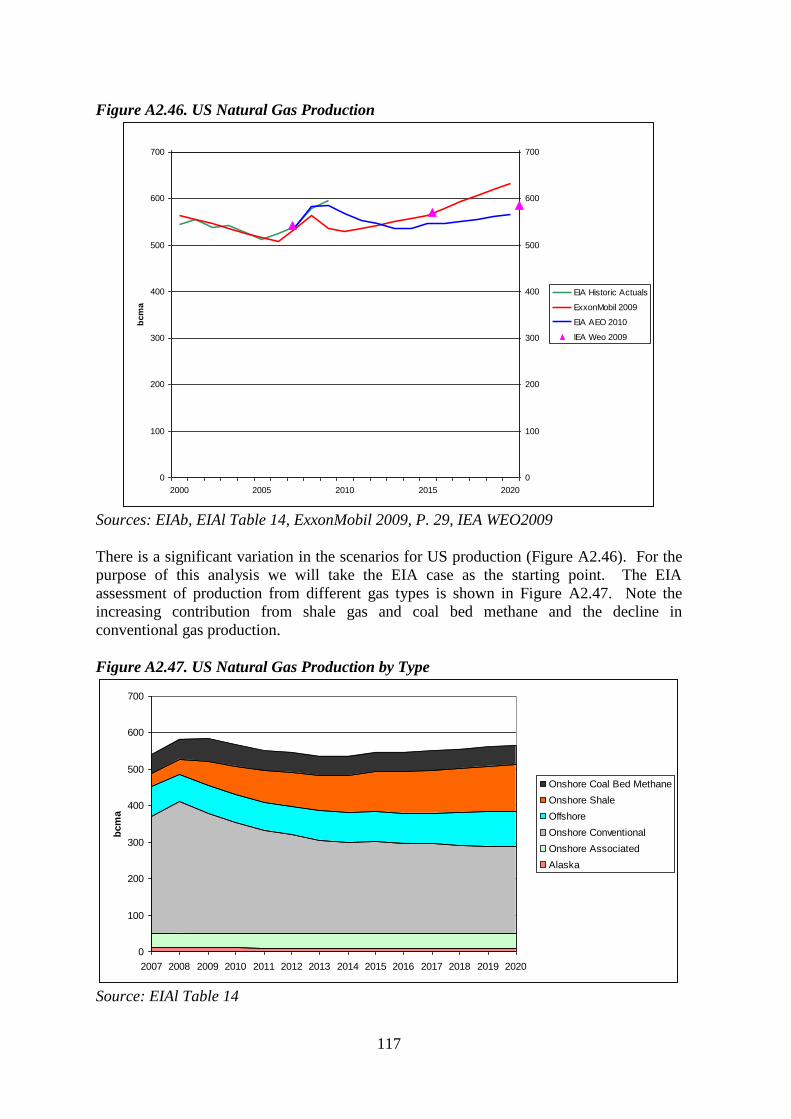
117
Figure A2.46. US Natural Gas Production
0
100
200
300
400
500
600
700
2000 2005 2010 2015 2020
bcm
a
0
100
200
300
400
500
600
700
2000 2020
EIA Historic Actuals
ExxonMobil 2009
EIA AEO 2010
IEA Weo 2009
Sources: EIAb, EIAl Table 14, ExxonMobil 2009, P. 29, IEA WEO2009
There is a significant variation in the scenarios for US production (Figure A2.46). For the
purpose of this analysis we will take the EIA case as the starting point. The EIA
assessment of production from different gas types is shown in Figure A2.47. Note the
increasing contribution from shale gas and coal bed methane and the decline in
conventional gas production.
Figure A2.47. US Natural Gas Production by Type
0
100
200
300
400
500
600
700
2007 2008 2009 2010 2011 2012 2013 2014 2015 2016 2017 2018 2019 2020
bcm
a
Onshore Coal Bed Methane
Onshore Shale
Offshore
Onshore Conventional
Onshore Associated
Alaska
Source: EIAl Table 14

118
Figure A2.48. Canadian Natural Gas Production
0
20
40
60
80
100
120
140
160
180
200
2000 2005 2010 2015 2020
bcm
a
IEA WEO2009
CGA
Assumption
IEA Actual
EIA IEO 2009
Sources: IEA Monthly Data Series, IEA WEO 2009, CGA 2009 P 2, Figure 1, EIAj
Canadian production is shown in Figure A2.48. All sources envisage the decline in
Canadian production, which began in 2007, continuing until around 2015. An average of
future views was taken for this analysis. This is shown as the light green line.
Figure A2.49. Mexican Natural Gas Production
0
10
20
30
40
50
60
70
2000
2001
2002
2003
2004
2005
2006
2007
2008
2009
2010
2011
2012
2013
2014
2015
2016
2017
2018
2019
2020
bcm
a
Assumption
IEA WEO2009
IEA Actual
EIA IEO 2009
Sources: EIAj, IEA Monthly Data Series, IEA WEO 2009

119
Figure A2.49 shows scenarios for Mexican gas production from the EIA and IEA. An
average of the two was taken for this analysis (shown as light green).
The annual production forecasts derived in this section for the US and Canada should be
considered merely as a „starting point‟. These will be revised as a consequence of the
model framework later in this Chapter, in response to price dynamics induced by LNG
arbitrage.
Storage capacity
As we noted in Chapter 1, storage inventory is a key indicator of impending shortage or
surplus of natural gas supply in the North American market. In Chapter 2 the framework
description clearly identifies US and Canadian storage as the de-facto short term balancing
mechanism for global LNG shortage or surplus. Figure A2.50 shows the pattern of end-
month storage inventory for the US and Canada in the period 2000 to the present (Canadian
data available from January 2003).
A recent assessment of US working gas storage capacity41
undertaken under the auspices of
the EIA placed this in the range 110 to 122 bcm (3,889 to 4,313 bcf). It was noted that
these figures had risen by 2.6% and 4.3% respectively since a similar assessment had been
undertaken in 2008. No comparable assessment for Canadian storage was found however
adding the maximum observed storage value (17.4 bcm for November 2009) gives a range
for US and Canada combined of 127.5 bcm to 139.5 bcm. The mid point of this range
(133.5 bcm) is shown on Figure A2.50 as an indicative maximum capacity.
Figure A2.50. US and Canada End Month Storage Working Gas Capacity
-
20,000
40,000
60,000
80,000
100,000
120,000
140,000
160,000
Jan-
00
Jul-0
0
Jan-
01
Jul-0
1
Jan-
02
Jul-0
2
Jan-
03
Jul-0
3
Jan-
04
Jul-0
4
Jan-
05
Jul-0
5
Jan-
06
Jul-0
6
Jan-
07
Jul-0
7
Jan-
08
Jul-0
8
Jan-
09
Jul-0
9
mc
m
US Canada Total Estimated Maximum Capacity
Sources: EIAe, CGA, La Rose 2009
Re-Gas Capacity
The US, Canada and Mexico have since year 2000 built significant LNG regas capacity
which at end 2009 is estimated to total some 150 bcma. Regas capacity is highly unlikely
to present a bottleneck to LNG imports in the decade to come.
41
La Rose 2009

120
LNG Niche Markets
In addition to the established LNG markets described previously, there are several „niche‟
or new LNG markets which whilst unlikely to directly influence LNG arbitrage dynamics
do need to be accounted for, in terms of their consumption of part of the global LNG
supply „pool‟. The Dominican Republic and Puerto Rica have been small but consistent
LNG consumers since the early 2000s. In South America Argentina, Brazil and Chile have
commenced imports. In the Middle East Kuwait has commenced imports and is likely to
be followed by Dubai from 2010 onwards. In addition schemes are likely for South Africa,
Cyprus, Thailand and Singapore. An annual estimate of demand from these markets is
shown in Figure A2.51.
Figure A2.51. New LNG Market Annual Demand
0
5
10
15
20
25
30
35
2005 2006 2007 2008 2009 2010 2011 2012 2013 2014 2015 2016 2017 2018 2019 2020
bc
ma
Dubai
Kuwait
South Africa
Chile
Brazil
Argentina
Cyprus
Thailand
Singapore
Puerto Rico
Dominican Republic
Sources: Waterborne LNG, Company Reports, Author’s Analysis
Demand for LNG for these markets is difficult to predict as in most cases it is acting as a
supplementary supply to indigenous production and/or pipeline imports. An additional
complexity lies in the fact that many of these markets are likely to be seasonal LNG
importers.
Global LNG Supply
The past and future LNG liquefaction picture has been assembled from a variety of natural
gas media sources and is shown in Figure A2.52.
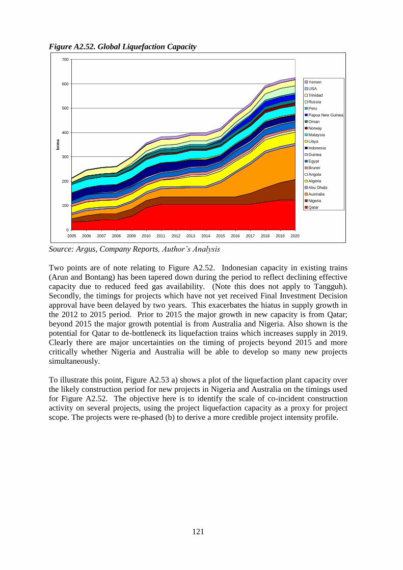
121
Figure A2.52. Global Liquefaction Capacity
0
100
200
300
400
500
600
700
2005 2006 2007 2008 2009 2010 2011 2012 2013 2014 2015 2016 2017 2018 2019 2020
bcm
a
Yemen
USA
Trinidad
Russia
Peru
Papua New Guinea
Oman
Norway
Malaysia
Libya
Indonesia
Guinea
Egypt
Brunei
Angola
Algeria
Abu Dhabi
Australia
Nigeria
Qatar
Source: Argus, Company Reports, Author’s Analysis
Two points are of note relating to Figure A2.52. Indonesian capacity in existing trains
(Arun and Bontang) has been tapered down during the period to reflect declining effective
capacity due to reduced feed gas availability. (Note this does not apply to Tangguh).
Secondly, the timings for projects which have not yet received Final Investment Decision
approval have been delayed by two years. This exacerbates the hiatus in supply growth in
the 2012 to 2015 period. Prior to 2015 the major growth in new capacity is from Qatar;
beyond 2015 the major growth potential is from Australia and Nigeria. Also shown is the
potential for Qatar to de-bottleneck its liquefaction trains which increases supply in 2019.
Clearly there are major uncertainties on the timing of projects beyond 2015 and more
critically whether Nigeria and Australia will be able to develop so many new projects
simultaneously.
To illustrate this point, Figure A2.53 a) shows a plot of the liquefaction plant capacity over
the likely construction period for new projects in Nigeria and Australia on the timings used
for Figure A2.52. The objective here is to identify the scale of co-incident construction
activity on several projects, using the project liquefaction capacity as a proxy for project
scope. The projects were re-phased (b) to derive a more credible project intensity profile.

122
Figure A2.53. Nigerian and Australian LNG Project Intensity and Re-phasing.
a) Project Timings as in Figure 107
Nigeria
0
10
20
30
40
50
60
2005 2010 2015 2020
bcm
a OKLNG Expansion
OloKolaLNGBrass River
NLNG T7
Australia
0
20
40
60
80
100
120
140
2005 2010 2015 2020
bcm
a
Scarborough/Pilbara
Gladstone 1
Wheatstone
Gladstone Santos
Australia Pacific LNG
BG Curtis Island
Browse
Greater Sunrise
Pluto
Icthys
Gorgon T2
Gorgon T1
b) Revised Project Timings
Nigeria Revised
0
10
20
30
40
50
60
2005 2010 2015 2020
bcm
a OKLNG Expansion
OloKolaLNG
Brass River
NLNG T7
Australia Revised
0
20
40
60
80
100
120
140
2005 2010 2015 2020
bcm
a
Scarborough/Pilbara
Gladstone 1
Wheatstone
Gladstone Santos
Australia Pacific LNG
BG Curtis Island
Browse
Greater Sunrise
Pluto
Icthys
Gorgon T2
Gorgon T1
a) Project Timings as in Figure 126
Nigeria
0
10
20
30
40
50
60
2005 2010 2015 2020
bcm
a OKLNG Expansion
OloKolaLNGBrass River
NLNG T7
Nigeria
0
10
20
30
40
50
60
2005 2010 2015 2020
bcm
a OKLNG Expansion
OloKolaLNGBrass River
NLNG T7
Australia
0
20
40
60
80
100
120
140
2005 2010 2015 2020
bcm
a
Scarborough/Pilbara
Gladstone 1
Wheatstone
Gladstone Santos
Australia Pacific LNG
BG Curtis Island
Browse
Greater Sunrise
Pluto
Icthys
Gorgon T2
Gorgon T1
Australia
0
20
40
60
80
100
120
140
2005 2010 2015 2020
bcm
a
Scarborough/Pilbara
Gladstone 1
Wheatstone
Gladstone Santos
Australia Pacific LNG
BG Curtis Island
Browse
Greater Sunrise
Pluto
Icthys
Gorgon T2
Gorgon T1
b) Revised Project Timings
Nigeria Revised
0
10
20
30
40
50
60
2005 2010 2015 2020
bcm
a OKLNG Expansion
OloKolaLNG
Brass River
NLNG T7
Nigeria Revised
0
10
20
30
40
50
60
2005 2010 2015 2020
bcm
a OKLNG Expansion
OloKolaLNG
Brass River
NLNG T7
Australia Revised
0
20
40
60
80
100
120
140
2005 2010 2015 2020
bcm
a
Scarborough/Pilbara
Gladstone 1
Wheatstone
Gladstone Santos
Australia Pacific LNG
BG Curtis Island
Browse
Greater Sunrise
Pluto
Icthys
Gorgon T2
Gorgon T10
20
40
60
80
100
120
140
2005 2010 2015 2020
bcm
a
Scarborough/Pilbara
Gladstone 1
Wheatstone
Gladstone Santos
Australia Pacific LNG
BG Curtis Island
Browse
Greater Sunrise
Pluto
Icthys
Gorgon T2
Gorgon T1
a) Project Timings as in Figure 107
Nigeria
0
10
20
30
40
50
60
2005 2010 2015 2020
bcm
a OKLNG Expansion
OloKolaLNGBrass River
NLNG T7
Nigeria
0
10
20
30
40
50
60
2005 2010 2015 2020
bcm
a OKLNG Expansion
OloKolaLNGBrass River
NLNG T7
Australia
0
20
40
60
80
100
120
140
2005 2010 2015 2020
bcm
a
Scarborough/Pilbara
Gladstone 1
Wheatstone
Gladstone Santos
Australia Pacific LNG
BG Curtis Island
Browse
Greater Sunrise
Pluto
Icthys
Gorgon T2
Gorgon T1
Australia
0
20
40
60
80
100
120
140
2005 2010 2015 2020
bcm
a
Scarborough/Pilbara
Gladstone 1
Wheatstone
Gladstone Santos
Australia Pacific LNG
BG Curtis Island
Browse
Greater Sunrise
Pluto
Icthys
Gorgon T2
Gorgon T1
b) Revised Project Timings
Nigeria Revised
0
10
20
30
40
50
60
2005 2010 2015 2020
bcm
a OKLNG Expansion
OloKolaLNG
Brass River
NLNG T7
Nigeria Revised
0
10
20
30
40
50
60
2005 2010 2015 2020
bcm
a OKLNG Expansion
OloKolaLNG
Brass River
NLNG T7
Australia Revised
0
20
40
60
80
100
120
140
2005 2010 2015 2020
bcm
a
Scarborough/Pilbara
Gladstone 1
Wheatstone
Gladstone Santos
Australia Pacific LNG
BG Curtis Island
Browse
Greater Sunrise
Pluto
Icthys
Gorgon T2
Gorgon T10
20
40
60
80
100
120
140
2005 2010 2015 2020
bcm
a
Scarborough/Pilbara
Gladstone 1
Wheatstone
Gladstone Santos
Australia Pacific LNG
BG Curtis Island
Browse
Greater Sunrise
Pluto
Icthys
Gorgon T2
Gorgon T1
a) Project Timings as in Figure A2.52
Nigeria
0
10
20
30
40
50
60
2005 2010 2015 2020
bcm
a OKLNG Expansion
OloKolaLNGBrass River
NLNG T7
Nigeria
0
10
20
30
40
50
60
2005 2010 2015 2020
bcm
a OKLNG Expansion
OloKolaLNGBrass River
NLNG T7
Australia
0
20
40
60
80
100
120
140
2005 2010 2015 2020
bcm
a
Scarborough/Pilbara
Gladstone 1
Wheatstone
Gladstone Santos
Australia Pacific LNG
BG Curtis Island
Browse
Greater Sunrise
Pluto
Icthys
Gorgon T2
Gorgon T1
Australia
0
20
40
60
80
100
120
140
2005 2010 2015 2020
bcm
a
Scarborough/Pilbara
Gladstone 1
Wheatstone
Gladstone Santos
Australia Pacific LNG
BG Curtis Island
Browse
Greater Sunrise
Pluto
Icthys
Gorgon T2
Gorgon T1
b) Revised Project Timings
Nigeria Revised
0
10
20
30
40
50
60
2005 2010 2015 2020
bcm
a OKLNG Expansion
OloKolaLNG
Brass River
NLNG T7
Nigeria Revised
0
10
20
30
40
50
60
2005 2010 2015 2020
bcm
a OKLNG Expansion
OloKolaLNG
Brass River
NLNG T7
Australia Revised
0
20
40
60
80
100
120
140
2005 2010 2015 2020
bcm
a
Scarborough/Pilbara
Gladstone 1
Wheatstone
Gladstone Santos
Australia Pacific LNG
BG Curtis Island
Browse
Greater Sunrise
Pluto
Icthys
Gorgon T2
Gorgon T10
20
40
60
80
100
120
140
2005 2010 2015 2020
bcm
a
Scarborough/Pilbara
Gladstone 1
Wheatstone
Gladstone Santos
Australia Pacific LNG
BG Curtis Island
Browse
Greater Sunrise
Pluto
Icthys
Gorgon T2
Gorgon T1
Gorgon T2
Gorgon T1Gorgon T1
a) Project Timings as in Figure 107
Nigeria
0
10
20
30
40
50
60
2005 2010 2015 2020
bcm
a OKLNG Expansion
OloKolaLNGBrass River
NLNG T7
Nigeria
0
10
20
30
40
50
60
2005 2010 2015 2020
bcm
a OKLNG Expansion
OloKolaLNGBrass River
NLNG T7
Australia
0
20
40
60
80
100
120
140
2005 2010 2015 2020
bcm
a
Scarborough/Pilbara
Gladstone 1
Wheatstone
Gladstone Santos
Australia Pacific LNG
BG Curtis Island
Browse
Greater Sunrise
Pluto
Icthys
Gorgon T2
Gorgon T1
Australia
0
20
40
60
80
100
120
140
2005 2010 2015 2020
bcm
a
Scarborough/Pilbara
Gladstone 1
Wheatstone
Gladstone Santos
Australia Pacific LNG
BG Curtis Island
Browse
Greater Sunrise
Pluto
Icthys
Gorgon T2
Gorgon T1
b) Revised Project Timings
Nigeria Revised
0
10
20
30
40
50
60
2005 2010 2015 2020
bcm
a OKLNG Expansion
OloKolaLNG
Brass River
NLNG T7
Nigeria Revised
0
10
20
30
40
50
60
2005 2010 2015 2020
bcm
a OKLNG Expansion
OloKolaLNG
Brass River
NLNG T7
Australia Revised
0
20
40
60
80
100
120
140
2005 2010 2015 2020
bcm
a
Scarborough/Pilbara
Gladstone 1
Wheatstone
Gladstone Santos
Australia Pacific LNG
BG Curtis Island
Browse
Greater Sunrise
Pluto
Icthys
Gorgon T2
Gorgon T10
20
40
60
80
100
120
140
2005 2010 2015 2020
bcm
a
Scarborough/Pilbara
Gladstone 1
Wheatstone
Gladstone Santos
Australia Pacific LNG
BG Curtis Island
Browse
Greater Sunrise
Pluto
Icthys
Gorgon T2
Gorgon T1
a) Project Timings as in Figure 126
Nigeria
0
10
20
30
40
50
60
2005 2010 2015 2020
bcm
a OKLNG Expansion
OloKolaLNGBrass River
NLNG T7
Nigeria
0
10
20
30
40
50
60
2005 2010 2015 2020
bcm
a OKLNG Expansion
OloKolaLNGBrass River
NLNG T7
Australia
0
20
40
60
80
100
120
140
2005 2010 2015 2020
bcm
a
Scarborough/Pilbara
Gladstone 1
Wheatstone
Gladstone Santos
Australia Pacific LNG
BG Curtis Island
Browse
Greater Sunrise
Pluto
Icthys
Gorgon T2
Gorgon T1
Australia
0
20
40
60
80
100
120
140
2005 2010 2015 2020
bcm
a
Scarborough/Pilbara
Gladstone 1
Wheatstone
Gladstone Santos
Australia Pacific LNG
BG Curtis Island
Browse
Greater Sunrise
Pluto
Icthys
Gorgon T2
Gorgon T1
b) Revised Project Timings
Nigeria Revised
0
10
20
30
40
50
60
2005 2010 2015 2020
bcm
a OKLNG Expansion
OloKolaLNG
Brass River
NLNG T7
Nigeria Revised
0
10
20
30
40
50
60
2005 2010 2015 2020
bcm
a OKLNG Expansion
OloKolaLNG
Brass River
NLNG T7
Australia Revised
0
20
40
60
80
100
120
140
2005 2010 2015 2020
bcm
a
Scarborough/Pilbara
Gladstone 1
Wheatstone
Gladstone Santos
Australia Pacific LNG
BG Curtis Island
Browse
Greater Sunrise
Pluto
Icthys
Gorgon T2
Gorgon T10
20
40
60
80
100
120
140
2005 2010 2015 2020
bcm
a
Scarborough/Pilbara
Gladstone 1
Wheatstone
Gladstone Santos
Australia Pacific LNG
BG Curtis Island
Browse
Greater Sunrise
Pluto
Icthys
Gorgon T2
Gorgon T1
Gorgon T2
Gorgon T1Gorgon T1
a) Project Timings as in Figure 107
Nigeria
0
10
20
30
40
50
60
2005 2010 2015 2020
bcm
a OKLNG Expansion
OloKolaLNGBrass River
NLNG T7
Nigeria
0
10
20
30
40
50
60
2005 2010 2015 2020
bcm
a OKLNG Expansion
OloKolaLNGBrass River
NLNG T7
Australia
0
20
40
60
80
100
120
140
2005 2010 2015 2020
bcm
a
Scarborough/Pilbara
Gladstone 1
Wheatstone
Gladstone Santos
Australia Pacific LNG
BG Curtis Island
Browse
Greater Sunrise
Pluto
Icthys
Gorgon T2
Gorgon T1
Australia
0
20
40
60
80
100
120
140
2005 2010 2015 2020
bcm
a
Scarborough/Pilbara
Gladstone 1
Wheatstone
Gladstone Santos
Australia Pacific LNG
BG Curtis Island
Browse
Greater Sunrise
Pluto
Icthys
Gorgon T2
Gorgon T1
b) Revised Project Timings
Nigeria Revised
0
10
20
30
40
50
60
2005 2010 2015 2020
bcm
a OKLNG Expansion
OloKolaLNG
Brass River
NLNG T7
Nigeria Revised
0
10
20
30
40
50
60
2005 2010 2015 2020
bcm
a OKLNG Expansion
OloKolaLNG
Brass River
NLNG T7
Australia Revised
0
20
40
60
80
100
120
140
2005 2010 2015 2020
bcm
a
Scarborough/Pilbara
Gladstone 1
Wheatstone
Gladstone Santos
Australia Pacific LNG
BG Curtis Island
Browse
Greater Sunrise
Pluto
Icthys
Gorgon T2
Gorgon T10
20
40
60
80
100
120
140
2005 2010 2015 2020
bcm
a
Scarborough/Pilbara
Gladstone 1
Wheatstone
Gladstone Santos
Australia Pacific LNG
BG Curtis Island
Browse
Greater Sunrise
Pluto
Icthys
Gorgon T2
Gorgon T1
a) Project Timings as in Figure A2.52
Nigeria
0
10
20
30
40
50
60
2005 2010 2015 2020
bcm
a OKLNG Expansion
OloKolaLNGBrass River
NLNG T7
Nigeria
0
10
20
30
40
50
60
2005 2010 2015 2020
bcm
a OKLNG Expansion
OloKolaLNGBrass River
NLNG T7
Australia
0
20
40
60
80
100
120
140
2005 2010 2015 2020
bcm
a
Scarborough/Pilbara
Gladstone 1
Wheatstone
Gladstone Santos
Australia Pacific LNG
BG Curtis Island
Browse
Greater Sunrise
Pluto
Icthys
Gorgon T2
Gorgon T1
Australia
0
20
40
60
80
100
120
140
2005 2010 2015 2020
bcm
a
Scarborough/Pilbara
Gladstone 1
Wheatstone
Gladstone Santos
Australia Pacific LNG
BG Curtis Island
Browse
Greater Sunrise
Pluto
Icthys
Gorgon T2
Gorgon T1
b) Revised Project Timings
Nigeria Revised
0
10
20
30
40
50
60
2005 2010 2015 2020
bcm
a OKLNG Expansion
OloKolaLNG
Brass River
NLNG T7
Nigeria Revised
0
10
20
30
40
50
60
2005 2010 2015 2020
bcm
a OKLNG Expansion
OloKolaLNG
Brass River
NLNG T7
Australia Revised
0
20
40
60
80
100
120
140
2005 2010 2015 2020
bcm
a
Scarborough/Pilbara
Gladstone 1
Wheatstone
Gladstone Santos
Australia Pacific LNG
BG Curtis Island
Browse
Greater Sunrise
Pluto
Icthys
Gorgon T2
Gorgon T10
20
40
60
80
100
120
140
2005 2010 2015 2020
bcm
a
Scarborough/Pilbara
Gladstone 1
Wheatstone
Gladstone Santos
Australia Pacific LNG
BG Curtis Island
Browse
Greater Sunrise
Pluto
Icthys
Gorgon T2
Gorgon T1Gorgon T1
Gorgon T2
Gorgon T1Gorgon T1
Source: Argus, Company Reports, Author’s Analysis
The revised project timings were used to construct the annual liquefaction capacity shown
in Figure A2.54 and used as the basis of evaluating supply.
Figure A2.54. Global Liquefaction Capacity with Re-Phasing
0
100
200
300
400
500
600
700
2005 2006 2007 2008 2009 2010 2011 2012 2013 2014 2015 2016 2017 2018 2019 2020
bcm
a
Yemen
USA
Trinidad
Russia
Peru
Papua New Guinea
Oman
Norway
Malaysia
Libya
Indonesia
Guinea
Egypt
Brunei
Angola
Algeria
Abu Dhabi
Australia
Nigeria
Qatar
Source: Argus, Company Reports, Author’s Analysis

123
The challenge is now to translate a view of annual liquefaction capacity into a forecast of
monthly LNG supply. The three elements in this process are described in outline below:
Monthly throughput variances
Although the general financial imperative is for liquefaction plants to operate at maximum
throughput all year round, two factors prevent this from actually occurring in reality:
Higher ambient temperatures reduce the output of the liquefaction plant making actual
output seasonal in shape.
Maintenance shutdowns periodically take plant out of service.
Looking at historic actual data at a supply country level enables an „average monthly
profile‟ to be derived – as a ratio of nameplate liquefaction plant capacity.
Commissioning Curves
When a new liquefaction plant is brought into service it may take several months before it
reaches design capacity. While specific data is not generally available in the public
domain, the assumption used in this analysis is that the plant begins operation at 25% of
capacity, reaches 90% after 6 months and 100% after 12 months.
Ad-hoc Underperformance/Overview
Prior to 2006 liquefaction plant reliability was regarded as high. With the trend to larger
trains since this time, we have seen several examples where plants have suffered downtime
either due to technical problems or gas availability problems. These need to be factored in
as specific assumptions.
Combining these steps allows us to assemble a forecast for global LNG supply at a monthly
level of detail. This is shown in Figure A2.55 together with the nameplate capacity and a
comparison of forecast and actual output for the historic period.
Note that there is a good match between forecast and historical values up until January
2009. Nigeria and Algeria suffered liquefaction and/or feed gas problems and declared
contractual Force Majeure during 2009 which in large part explains the difference between
forecast and historical values. The last three months of 2009 however show encouraging
agreement between forecast and actual. A key feature of this chart is the significant ramp-
up in LNG volumes from October 2009 when the commissioning of new LNG trains
reinforces the normal seasonal increase in LNG output.

124
Figure A2.55. Monthly Global LNG Supply
-
200
400
600
800
1,000
1,200
1,400
1,600
1,800
Ja
n-0
5
Ja
n-0
6
Ja
n-0
7
Ja
n-0
8
Ja
n-0
9
Ja
n-1
0
Ja
n-1
1
Ja
n-1
2
Ja
n-1
3
Ja
n-1
4
Ja
n-1
5
Ja
n-1
6
Ja
n-1
7
Ja
n-1
8
Ja
n-1
9
Ja
n-2
0
mc
m/d
ay
Predicted Actual Nameplate Capacity
Sources: Waterborne LNG, Author’s Analysis
125
Bibliography
Argus: Argus Global LNG price series, monthly subscription service containing price data
on contracted and spot LNG and pipeline gas.
Baker Hughes 2009: Baker Hughes Website: North American Rotary Rig Count download
at http://investor.shareholder.com/bhi/rig_counts/rc_index.cfm;
BP 2009: BP Statistical Review of World Energy 2009. This is an annual review from
which data can be downloaded at:
http://www.bp.com/productlanding.do?categoryId=6929&contentId=7044622
Data for LNG and Pipeline trade for years prior to 2008 are contained in previous annual
editions of the BP Statistical Review.
Bradley, Angell, McManus 2008: REPORT: DomGas Alliance Group, WA Midstream
Gathering and Processing Review with Global Analogues, March, 2008, David Bradley /
Ian Angell / Andrew McManus Wood Mackenzie,
http://www.pc.gov.au/data/assets/pdf_file/0004/82498/sub001-attachment1.pdf
Cedigaz 2004: LNG Trade and Infrastructures, Cedigaz, February 2004.
Cedigas 2008: Pipeline Long Term Gas Contracts by Exporter, Cedigaz, Armelle
Lecarpentier, August 2008.
Cedigaz & BP : Cedigaz Historic Pipeline Trade Data as published in the annual BP
Statistical Review of World Energy.
CGA: Canadian Gas Association website:
http://www.cga.ca/publications/documents/Chart11-NaturalGasStorage.pdf
CGA 2009: „North American Gas Supply: Increasingly Unconventional‟, Association
Canadienne de Gaz, September 2009. http://www.cga.ca/publications/documents/UpdatedsupplybulletinAugust2009.pdf
EIAa: EIA Electric Power Annual 2007, January 21st 2009. Table 2.1.
http://www.eia.doe.gov/cneaf/electricity/epa/epa_sum.html#two
EIAb: EIA Website: US gas production, storage and demand data downloads at
http://tonto.eia.doe.gov/dnav/ng/ng_prod_sum_dcu_NUS_m.htm
EIAc: Major Legislative and Regulatory Actions (1935 – 2008), Released January 30th
2009,
http://www.eia.doe.gov/oil_gas/natural_gas/analysis_publications/ngmajorleg/ngmajorleg.
html
EIAd: EIA Natural Gas Statistics; import and export tables.
http://www.eia.doe.gov/oil_gas/natural_gas/info_glance/natural_gas.html
126
EAIe: EIA Storage working gas inventory data .
http://tonto.eia.doe.gov/dnav/ng/hist/n5020us2m.htm
EIAf: EIAdata on power generation fuels
http://www.eia.doe.gov/cneaf/electricity/epm/epm_sum.html
EIAg: Table of Net Generation by Energy Source: http://www.eia.doe.gov/cneaf/electricity/epm/table1_1.html,
EIAh: Fuel prices from download at: http://tonto.eia.doe.gov/dnav/pet/hist/a313600002m.htm
EIAi: Storage working gas inventory data at:
http://tonto.eia.doe.gov/dnav/ng/ng_stor_sum_dcu_nus_m.htm
EIAj: The EIA‟s 2009 assessment of international gas production is available at:
http://www.eia.doe.gov/emeu/international/gasproduction.html
EIAk: The EIA‟s 2009 assessment of international gas demand is available at:
http://www.eia.doe.gov/oiaf/ieo/ieorefcase.html
EIAl: The EIA‟s Annual Energy Outlook 2010 Early Release Overview
Report #:DOE/EIA-0383(2009), December 14, 2009
http://www.eia.doe.gov/oiaf/aeo/aeoref_tab.html
Eurostat Heating Degree Days: European heating degree day data at a national level.
http://epp.eurostat.ec.europa.eu/portal/page/portal/energy/data/database
ExxonMobil 2009: Outlook For Energy, a View to 2030, 2009
http://thomson.mobular.net/thomson/7/2946/4101/
FACTS 2008: FACTS Asian LNG Service which reports the prices paid for spot LNG
cargoes.
FEPC: Federation of Electric Power Companies of Japan website containing monthly
generation fuel consumption data at:
http://www.fepc.or.jp/english/news/generated_purchased/index.html
Flower 2009a: Article ‟More LNG for China, But will the Terminals be There to receive it
All?‟, Andy Flower, Waterborne LNG Asia Report 22nd
May 2009.
Flower 2009b: Article ‟What Next for LNG in India‟, Andy Flower, Waterborne LNG Asia
Report 19th
June 2009.
Flower 2009c: How Much More LNG Does Korea Need by 2020?, Article in Waterborne
LNG Asia Report, 9th October 2009.
Foss 2007: United States Natural Gas Prices to 2015, Michelle Michot Foss, Ph.D. OIES
NG18, February 2007.
http://www.oxfordenergy.org/pdfs/NG18.pdf

127
Futyan 2006: The Interconnector Pipeline A Key to Europe‟s Gas Network, Mark Futyan,
OIES, Marc 2006.
http://www.oxfordenergy.org/pdfs/NG11.pdf
Gas Matters: A daily subscription gas journal „Gas Matters Today‟, used as a source of
Average German Import Price in $/mmbtu. This data can also be accessed as a
downloadable spreadsheet (in €/Tj) from the German Federal Ministry of Economics and
Technology at:
http://www.bmwi.de/BMWi/Navigation/Service/publikationen,did=53736.html
Gas Strategies 2009: LNG Ship data from Gas Strategies LNG Database, March 2009
GSE: Website containing storage inventory data grouped by trading hub area at:
https://transparency.gie.eu.com/
Haase 2008: European Gas Market Liberalisation: Are regulatory regimes moving towards
convergence ?, Nadine Haase, OIES, May 2008.
http://www.oxfordenergy.org/books.php?&myflag=f&submit=Filter&searchfor=Gas
Honore (Forthcoming) 2010: European Gas Demand, Supply & Pricing: cycles, seasons
and the impact of LNG price arbitrage, Anouk Honore
ICE: ICE Futures Exchange
ICIS Heren: ICIS Heren Global LNG Markets: a subscription service which publishes a
monthly index of UK gas price.
IEA WEO 2009: The IEA World Energy Outlook, November 2009.
IEA Annual Data Series: This is a subscription service for annual data on European natural
gas demand by sector. http://data.iea.org/ieastore/statslisting.asp
IEA Monthly Data Series: This is a subscription service for monthly data on European
natural gas demand, production, imports, exports and national stock levels. When released,
data is usually three months old. http://data.iea.org/ieastore/statslisting.asp
IHS 2005: ‘Global Gas –Land of Opportunity?’,APPEX –March 02, 2005, Mark Stearnes
Director, Gas Consulting, IHS Energy
http://energy.ihs.com/NR/rdonlyres/8FB59668-D603-4A7F-8596-
36CE2C68820C/0/stearnes.pdf
IUK: Website of the UK – Belgium Interconnector pipeline operator from which historical
flowrate data may be downloaded
http://www.interconnector.com/onlineservices/historicflows.htm
Jensen: Oil-to-Gas Competition – Can it place a Cap on Gas Prices?
By James T. Jensen, undated
http://www.usaee.org/pdf/iaeemail.pdf
Jensen 2004: The Development of a Global LNG Market, James T Jensen, OIES, 2004.

128
Jensen 2009: LNG - Expanding the Horizons of International Gas Trade -- A Presentation
to the Spring Conference of the Association of International Petroleum Negotiators - New
Orleans May 1, 2009 .
http://www.jai-energy.com/index.php?page=pubs
La Rose 2009: „Estimates of Peak Underground Working Gas Storage Capacity in the
United States, 2009 Upate‟, Angelina La Rose, 2009.
http://www.eia.doe.gov/pub/oil_gas/natural_gas/feature_articles/2009/ngpeakstorage/ngpea
kstorage.pdf
Miyamoto & Ishiguro 2006: „Pricing and Demand for LNG in China: Consistency between
LNG and Pipeline Gas in a Fast Growing market‟, Akira Miyamoto and Chikako Ishiguro,
OIES January 2006. http://www.oxfordenergy.org/pdfs/NG9.pdf
National Grid: The operator of the UK‟s onshore gas and electricity distribution networks.
A UK future production forecast is included in the annual „Ten Year Statement‟ at:
http://www.nationalgrid.com/uk/Gas/
NPC 2003: „Balancing Natural Gas Policy‟, National Petroleum Council, September 2003.
http://www.npc.org/
NPD: The Norwegian Petroleum Directorate. The Resource Report 2009, 10th September
2009, Page 42.
http://www.npd.no/Global/Engelsk/3%20-
%20Publications/Resource%20report/Resource%20report%202009/Chapter%204.pdf
OGP: Future Netherlands gas production is shown in a graph on page 44 of a report
„Current and potential contribution of European oil and gas production to security of supply
in the EU‟, 2008, by the International Association of Oil and Gas Producers. http://www.nogepa.nl/images/08-07-16%20att.8a%20ogp%20paper%20on%20european%20production%20-
%20june%202008.pdf
OIES Asia 2008: Natural Gas In Asia, Edited by J Stern, Second Edition, OIES 2008,
Pirani 2009: „Russian and CIS gas markets and their impact on Europe‟, Edited by Simon
Pirani, OIES 2009.
Platts: a subscription energy markets service; used as a source of histroric Brent Crude
prices.
Poten 2008 : Potens & Partners Presentation: „The Outlook for Atlantic Basin LNG Supply
and Transportation‟, 14th Annual NECA Conference on Fuels Issues , Boston, MA,
September 24, 2008 http://www.necanews.org/dev/documents/080924mikhaiel_nelly.pdf
Reid 1999: „Deregulation of the Canadian Natural Gas Market‟, January 1999, Holly Reid,
Pages 2, 3, http://www.piac.ca/energy/deregulation_of_the_canadian_natural_gas_market/
Rosellon & Halpen 2001: „Regulatory Reform in Mexico s Natural Gas lndustry,
Liberalisation in the Context of a Dominant Upstream Incumbent‟, WP S A5 31 POLICY
RESEARCH WORKING PAPER 2537, World Bank January 2001, Juan Rosellon and

129
Jonathan Halpern,
http://econ.worldbank.org/external/default/main?print=Y&pagePK=64165259&theSitePK=
469382&piPK=64165421&menuPK=64166093&entityID=000094946_01021007442963
Smith 2005: Herbert Smith: Article: EU to punish restrictive business practices - An EU
competition law perspective on destination clauses in LNG contracts, 28th June 2005,
http://www.herbertsmith.com/NR/rdonlyres/57514EFE-4A32-42F6-AF96-
54F24845BF16/1149/euc_280605.html
Stern 2007: „Is there a rationale for the Continuing Link to Oil Product Prices in
Continental Europe Long Term Contracts?‟ Jonathan Stern, OIES, April 2007,
http://www.oxfordenergy.org/pdfs/NG19.pdf
UKOOA 2004: „Maximising Britain‟s Oil and Gas Resources‟ UK Offshore Operators
Economic Report 2004. http://www.ukooa.co.uk/issues/economic/econ04/pdf/summary.pdf
Vermier 2009: From a Presentation „Developments in the Global LNG Market. Would
Venezuela Find a Ready Market?‟ Jean Vermier, GIIGNL, 16th
April 2009.
http://www.venezuelagas.net/foro4/2.pdf
Waterborne LNG: Waterborne LNG is a subscription service providing US, European and
Asian reports data and commentary on LNG cargo movements. Data is reported at an
individual tanker level and summarised by month. In this way the complete global
supplier- importer matrix can be assembled at a monthly level. Data is available back to
January 2004.
Waterborne2009a: US Report 26th
June 2009.
Weather Underground: An open website providing historical temperature data at:
http://www.wunderground.com/history/airport/EGLL/2010/1/15/MonthlyHistory.html
WoodMac 2008a: WoodMackezie Global LNG Service 2008, data on existing, „in
development‟ and possible future LNG regasification terminals.
Wright 2006: Phillip Wright, Gas Prices in the UK: Markets and Insecurity of Supply,
Oxford University Press, 2006.
Zhuravleva 2009: The Nature of LNG Arbitrage, and an Analysis of the Main Barriers for the Growth of
the Global LNG Arbitrage Market, OIES, July 2009. http://www.oxfordenergy.org/pdfs/NG31.pdf

130
Glossary
AGIP: Average German Import Price of natural gas at the German border.
Annual Contract Quantity (ACQ): The quantity that, under a gas contract, a buyer has the
right to nominate and the seller the obligation to deliver.
Asia: In this paper Asia includes Pacific gas producers and consumers.
Associated Gas: Gas which is from a field which also produces oil.
BBL : shorthand for the Balgzand (Holland) to Bacton (UK) pipeline.
Bcf/d, bcf/d, bcfd: billion cubic feet per day. (equivalent to 10.34 bcma).
Bcma, bcma: billion cubic metres per annum.
Coal Bed Methane: methane which is held within the structure of the coal matrix by
adsorption. This may be produced in commercial quantities when the coal is de-
pressurised and de-watered in situ through drilling and the application of suitable well
technology.
Combined Cycle Gas Turbine (CCGT): a gas-fired power generation plant which has a
high pressure gas turbine cycle and a steam cycle.
Dry Gas: Natural gas which has had some of its naturally occurring components of ethane,
propane, butane and heavier hydrocarbon components removed through processing in order
to achieve sales specification.
Europe: As defined for the purpose of modelling in this paper Europe includes: Austria, ,
Belgium, Bulgaria, Croatia, Czech Republic, Denmark, Estonia, Finland, France, Germany,
Greece, Hungary, Ireland, Italy, Latvia, Lithuania Luxembourg, Netherlands, Norway,
Poland, Portugal, Romania, Serbia, Slovakia, Slovenia, Spain, Sweden, Switzerland,
Turkey, UK
FID: Final Investment Decision: usually in the context of an LNG project, this is the joint
decision on the part of the investment companies and any state entities to proceed with the full
development of a project through to commercial operation.
Force Majeure : is a common clause in contracts which essentially frees both parties
from liability or obligation when an extraordinary event or circumstance beyond the control of
the parties, such as a war, strike, riot, crime, or an event described by the legal term "act of
God" (e.g., flooding, earthquake, volcanic eruption), prevents one or both parties from fulfilling
their obligations under the contract. However, force majeure is not intended to
excuse negligence or other malfeasance of a party, as where non-performance is caused by the
usual and natural consequences of external forces, or where the intervening circumstances are
specifically contemplated.
Gas oil: refined petroleum fraction corresponding to diesel.
GW: Gigawatt, i.e. 1 billion watts

131
Hub : the location, physical or virtual, where a traded market for gas is established.
Henry Hub: Henry Hub is the pricing point for natural gas futures contracts traded on
the New York Mercantile Exchange (NYMEX). It is a point on the natural gas pipeline system
in Erath, Louisiana where it interconnects with nine interstate and four intrastate pipelines.
Spot and future prices set at Henry Hub are denominated in $/mmbtu (millions of British
thermal units) and are generally seen to be the primary price set for the North American natural
gas market.
IEA Europe : In terms of data on natural gas IEA Europe includes: Austria, , Belgium,
Czech Republic, Denmark, Finland, France, Germany, Greece, Hungary, Ireland, Italy,
Luxembourg, Netherlands, Norway, Poland, Portugal, Slovakia, Spain, Sweden,
Switzerland, Turkey, UK. The IEA is the International Energy Agency.
Independents: a term used to describe oil and gas companies which do not have the size
and scale of operations of the „majors‟. Historically they have tended to focus activities at
a national or continental level, but this is no longer necessarily the case.
Interstate Pipeline: a trunk pipeline carrying natural gas across US state boundaries.
IUK: the shorthand name for the Bacton (UK) to Zeebrugge (Belgium) bi-directional gas
pipeline, which is owned by Interconnector (UK) Ltd.
Linear Programming : Linear programming (LP) is a mathematical method for
determining a way to achieve the best outcome (such as maximum profit or lowest cost) in
a mathematical model for a list of requirements represented as linear equations
Liquefaction Plant: A large scale processing plant in which natural gas is cryogenically
cooled to minus 161° centigrade where it becomes a liquid at atmospheric pressure.
LNG: Liquefied Natural Gas
Local Distribution Company: a generic term for an organisation which purchases wholesale
natural gas at the „city gate‟ and sells it on a retail basis to end-users.
LSFO: Low Sulphur Fuel Oil
Mcm/day, mcm/day, mcm/d, mcmd: Million cubic metres per day.
MCM, mcm, mmcm; million cubic metres
Mmbtu: Million British thermal units
Mtce, mtce: million tonnes coal equivalent
Mtoe, mtoe: million tonnes oil equivalent (equivalent to 1.21 bcma of natural gas)
National Incumbent: a term to describe, usually in a European context, a natural gas
midstream company which currently or formerly enjoyed a monopoly position in the

132
supply chain either as an arm of the state or through the existence of a regulatory system in
which competition levels are/were low.
NBP: the UK‟s National Balancing Point: a virtual point (hub) in the National
Transmission System where gas trades are deemed to occur. It is also used as shorthand for
the UK spot gas price.
Normal year: A year in which ambient temperatures correspond to long range historical
averages.
North America: The USA, Canada and Mexico
Oil and Gas Majors: A term generally used to describe the group of the largest publicly
owned international oil and gas companies.
Oil Indexed Gas Prices: gas prices which are subject to contractual negotiation which are
determined by a formula (or formulae), containing rolling averages of crude oil or defined
oil products prices.
Productive Capacity: of gas wells, this relates to the maximum sustainable production
available from wells which are in existence. Production may be lower than this value if
some wells are being partially choked in.
Regas Terminal: (Regasification terminal) a terminal which receives LNG via an
unloading jetty and temporarily stores it in an insulated storage tank in liquid form. When
gas is required the LNG is gasified by providing a heat input prior to entering the
distribution grid.
Residual Fuel Oil: (Resid.) Heavy oils that are “leftovers” from various refining processes.
Most often used in marine boilers and in heating plants.
Rig Count: the number of rotary rigs which are actively drilling on a given date. These are
essentially working on exploration or development wells and represent the activity level of
new production capacity development.
Self Contracted: this refers to the situation where a participant commits to purchase
(usually) an annual quantity of LNG over a term of several years, backing it with a parent
company guarantee rather than a sales agreement with a specific customer. This allows the
participant to sell the gas flexibly in a range of geographical markets.
Shale Gas: natural gas formed in fine-grained shale rock (called gas shales) with low permeability
in which gas has been adsorbed by clay particles or is held within minute pores and microfractures.
Short Run Marginal Cost of Supply: the short run variable cost of gas production from
well-head to market. This would exclude any prior capital expenditure and any costs which
had been committed to under long term lease or contractual obligation.
Spot price: the price of gas determined through trading – i.e. determined by supply and
demand and/or gas on gas competition. Usually refers to as „prompt‟ rather than futures
prices.

133
Storage Inventory: the quantity of working gas volume in storage. Working gas is distinct
from „cushion gas‟ which is only withdrawn from storage when a storage site is
decommissioned.
Swing Field: a term used to describe a UK gas field where by virtue of a field-specific gas
sales contract signed with a buyer, the field is required to deliver significantly higher daily
volumes in winter than in summer.
Take or Pay (TOP): sometimes called the „minimum bill‟, this is the quantity of gas
which, during a gas contract year, a customer is obliged to pay for regardless of whether it
physically takes it for resale or not.
Tight Gas: natural gas found in sandstone or carbonate reservoirs (called tight gas sands) with low
permeability which prevents the gas from flowing naturally.
Wet Gas: gas which has not had its naturally occurring components of ethane, propane,
butane and heavier hydrocarbon components removed through processing.
Working Gas: see Storage Inventory.