load-based energy savings in three-phase squirrel cage
TRANSCRIPT

Graduate Theses, Dissertations, and Problem Reports
2004
Load-based energy savings in three-phase squirrel cage induction Load-based energy savings in three-phase squirrel cage induction
motors motors
Subodh Chaudhari West Virginia University
Follow this and additional works at: https://researchrepository.wvu.edu/etd
Recommended Citation Recommended Citation Chaudhari, Subodh, "Load-based energy savings in three-phase squirrel cage induction motors" (2004). Graduate Theses, Dissertations, and Problem Reports. 1530. https://researchrepository.wvu.edu/etd/1530
This Thesis is protected by copyright and/or related rights. It has been brought to you by the The Research Repository @ WVU with permission from the rights-holder(s). You are free to use this Thesis in any way that is permitted by the copyright and related rights legislation that applies to your use. For other uses you must obtain permission from the rights-holder(s) directly, unless additional rights are indicated by a Creative Commons license in the record and/ or on the work itself. This Thesis has been accepted for inclusion in WVU Graduate Theses, Dissertations, and Problem Reports collection by an authorized administrator of The Research Repository @ WVU. For more information, please contact [email protected].

Load Based Energy Savings in Three Phase Squirrel Cage Induction Motors
Subodh Chaudhari
Thesis submitted to the College of Engineering and Mineral Resources
At West Virginia University In partial fulfillment of the requirements
For the degree of
Master of Science In
Industrial Engineering
B. Gopalakrishnan, Ph.D., P.E., CEM Chair Ralph Plummer, Ph.D., P.E.
Parviz Famouri, Ph.D.
Department of Industrial and Management Systems Engineering
Morgantown, West Virginia 2004
Keywords: Induction Motors, Load Estimation, Slip Method, Input
Power Measurement, Motor Efficiency, Equivalent Circuit Parameters, Energy Savings

ABSTRACT
Load Based Energy Savings in Three Phase Squirrel Cage Induction Motors
Subodh Chaudhari
Chair Dr. B. Gopalakrishnan
Energy is an extremely valuable resource which should be used carefully. After
realizing this in the 1990’s DOE started various energy efficiency measures in order to
reduce the energy consumed by US industry. Motors use almost 50 percent of the
electricity in the United States. If motor efficiency could be increased then energy
consumption could be reduced. There have been efforts to increase motor efficiency over
past decade which lead to development of premium efficiency motors. Designed motor
efficiency is normally above 90 percent so motors do not waste energy. However, motor
efficiency decreases when load factor is less than 50 percent. Therefore measures need to
be taken to make the motor sizes properly fit the application load profile so as to improve
operational efficiency. Based on plant assessment experience plant personnel have very
limited data on motor loading. The decisions concerning motor sizing are usually based
on judgment or the slip method. Accurate load determination methods such as input
power measurement involve working around high voltages hence have safety issues.
These methods are time consuming and expensive. The purpose of this research was to
develop a method of sizing electric motors which is simple to use, economical, safe and
accurate. This research collected data during fifteen energy assessments conducted at
variety of facilities using the motor load monitoring method as well as by using a
stroboscope method. A statistical analysis of the data was conducted to determine if a
relationship exists between slip method and input power measurement load factors, so
that prediction of accurate load factor can be made based on the load factor obtained by
slip method. The model was built and validated based on mathematical and electrical
engineering principles.

AKNOWLEDGEMENT
I would like to wholeheartedly thank my advisor Dr. B. Gopalakrishnan and Dr.
P. Famouri for their continued support, guidance and encouragement during the course of
this research work. I also wish to thank Dr. Ralph Plummer for his advice and support.
Above all, I wish to thank god, my parents, my brother and all my friends for their
constant support and blessings and enabling my success and happiness in all my pursuits
and endeavors in life.
Lastly, I would like to again thank Dr. B. Gopalakrishnan, who encouraged me to
present a paper on part of this work in SPIE (International Society for Optical
Engineering) conference.
iii

Table of Contents
ABSTRACT....................................................................................................................... ii AKNOWLEDGEMENT.................................................................................................. iii 1 Introduction............................................................................................................... 1
1.1 Energy ................................................................................................................. 1 1.2 Electrical Motors, Their Importance & Electrical Energy.................................. 2
1.2.1 Applications of Induction Motors in Industry ............................................ 2 1.2.2 Usage of Induction Motors and Energy Consumed in Industry ................. 3 1.2.3 Energy and Dollars Wasted ........................................................................ 4
1.3 Need for Energy management ............................................................................ 6 1.4 Federal Energy Efficiency Initiative................................................................... 7 1.5 Basics of Induction Motors................................................................................. 9
1.5.1 Construction.............................................................................................. 10 1.5.2 Types of Induction Motors........................................................................ 10 1.5.3 NEMA Design Motors.............................................................................. 11
1.6 DC Motors ........................................................................................................ 12 1.6.1 Power Losses in DC Motors ..................................................................... 14 1.6.2 Energy Efficient DC Motor Drive ............................................................ 15
1.7 Mathematical Relations in Induction Motors ................................................... 15 1.8 Slip in Induction Motors ................................................................................... 18 1.9 Load Factor Evaluation..................................................................................... 19
1.9.1 Reasons to Determine Motor Loading...................................................... 19 1.9.2 Methods to Determine Load ..................................................................... 21
1.10 Potential for Energy Savings ............................................................................ 24 1.11 Need for research .............................................................................................. 24
1.11.1 Present Motor Loading in Industry ........................................................... 24 1.12 Objectives of Research ..................................................................................... 26 1.13 Conclusion ........................................................................................................ 26
2 Literature Review ................................................................................................... 27 2.1 Energy Conservation Measures for Induction Motors...................................... 27 2.2 Losses in Motor................................................................................................. 28 2.3 Efficiency Estimation........................................................................................ 29
2.3.1 Efficiency Testing Standards .................................................................... 29 2.3.2 Efficiency Determination.......................................................................... 30
2.4 Motor Nameplate Efficiency Labeling ............................................................. 33 2.5 Power Factor Improvement............................................................................... 34
2.5.1 Causes of Low Power Factor .................................................................... 35 2.5.2 Techniques to Improve Power Factor ....................................................... 36
2.6 Motor Repair and Motor Rewind...................................................................... 37 2.6.1 Impact of Rewinding on Motor Efficiency............................................... 37
2.7 Supermizer – Energy Saving System................................................................ 39 2.8 Conclusion ........................................................................................................ 40
3 Research Approach................................................................................................. 41 3.1 Collection of Field Data.................................................................................... 41
3.1.1 Required Data ........................................................................................... 41 3.1.2 Restriction on Data Collection.................................................................. 45
iv

3.1.3 Procedure for Data Collection .................................................................. 46 3.1.4 Collected Motor Data................................................................................ 49
3.2 Data Analysis .................................................................................................... 50 3.2.1 Load Factor Evaluation by Slip Method................................................... 50 3.2.2 Load Factor Evaluation by Voltage Corrected Slip Method .................... 50 3.2.3 Load Factor Evaluation by Line Current Measurement Method .............. 51 3.2.4 Load Factor Evaluation by Input Power Measurement ............................ 51
3.3 Results............................................................................................................... 54 3.3.1 Motor Loading In the Study Carried Out In the Field .............................. 54 3.3.2 Load Factors Relationships....................................................................... 56 3.3.3 Motor Energy & Demand Savings............................................................ 60
3.4 Conclusion ........................................................................................................ 64 4 Statistical Analysis and Model Development ....................................................... 65
4.1 Outline of Statistical Data Analysis.................................................................. 65 4.2 Data Collection & Preparation.......................................................................... 66
4.2.1 Elimination of Unnecessary Variables...................................................... 66 4.2.2 Removal of Outliers.................................................................................. 68 4.2.3 Data Splitting ............................................................................................ 68
4.3 Initial data trend spotting .................................................................................. 69 4.4 Model Building ................................................................................................. 71
4.4.1 Straight Line Model .................................................................................. 72 4.4.2 Polynomial Model..................................................................................... 75 4.4.3 Multiple Regression Model....................................................................... 78
4.5 Model Validation .............................................................................................. 91 4.6 Summary & Conclusion.................................................................................... 93
5 Load Factor Discrepancies and Other Considerations ....................................... 94 5.1 Reasons for under-loaded motors ..................................................................... 94
5.1.1 Application Need ...................................................................................... 94 5.1.2 Purchasing practices.................................................................................. 94 5.1.3 Aversion to Downtime.............................................................................. 95 5.1.4 Maintenance Practices .............................................................................. 95 5.1.5 Downsized Production.............................................................................. 96 5.1.6 Allowance for load growth ....................................................................... 96 5.1.7 Rounding up to the next size..................................................................... 96
5.2 Adjustable Speed Drives (ASD) ....................................................................... 97 5.2.1 Types of Adjustable Speed Drives............................................................ 98 5.2.2 Benefits of Using ASDs............................................................................ 99 5.2.3 Drawbacks of ASDs.................................................................................. 99 5.2.4 Applications of ASDs ............................................................................. 100
5.3 Discrepancies in Load Factors ........................................................................ 101 5.3.1 Slip Method............................................................................................. 101 5.3.2 Voltage Corrected Slip Method .............................................................. 102 5.3.3 Current Voltage Method ......................................................................... 103
5.4 Reasons for Load Factor Discrepancies.......................................................... 105 5.5 MATLAB GUI for torque-speed curve generation ........................................ 106 5.6 Validation of Statistical Model Built Considering Losses in Motor............... 109
v

5.7 Summary & Conclusion.................................................................................. 113 6 Conclusion and Future Work .............................................................................. 114
6.1 Conclusion ...................................................................................................... 114 6.2 Future Work .................................................................................................... 115
References...................................................................................................................... 117 APPENDIX I ................................................................................................................. 123 APPENDIX II................................................................................................................ 124 APPENDIX III .............................................................................................................. 127 APPENDIX IV .............................................................................................................. 132 APPENDIX V................................................................................................................ 137
vi

List of Figures
Figure 1.1 Energy Consumed by Oversized Motor vs. Properly Loaded Motor ................ 5 Figure 1.2 Cost Lost Due to Oversized Motor Over 10 Year Period.................................. 6 Figure 1.3 Relative shares of electrical input used by different motor types...................... 9 Figure 1.4 Torque of NEMA Design Motors .................................................................... 12 Figure 1.5 Optimal Efficiency Obtained by Controlling Field Current for Different
Operating Points .............................................................................................. 14 Figure 1.6 Efficiency and Power Factor Variation with Part Load on Motor................... 20 Figure 1.7 Percentage of Under-Loaded Motors in US industry ...................................... 25 Figure 2.1 Distribution of Induction Motor Losses........................................................... 28 Figure 2.2 Six Impedance per Phase Equivalent Circuit of an Induction Motor .............. 32 Figure 2.3 Power Factor Triangle...................................................................................... 34 Figure 2.4 Power Factor Variation with Load................................................................... 35 Figure 2.5 Capacitor Principle for Increasing Power Factor............................................. 36 Figure 2.6 Conceptual Configuration Diagram of Supermizer ......................................... 39 Figure 3.1 Principle of Stroboscope Speed Measurement ................................................ 47 Figure 3.2 3 Phase 3 wire Delta Connection Arrangement for Amprobe ......................... 48 Figure 3.3 DM II Pro 3 Phase 3 wire (Phase to Phase Measurement) Connections
Diagram ........................................................................................................... 48 Figure 3.4 Percentage of Motors According to Load Factor............................................. 54 Figure 3.5 Overall distribution of load factors in the tested motors.................................. 55 Figure 3.6 Slip Load Factor Vs Power Measurement Load Factor................................... 57 Figure 3.7 Relationship between voltage corrected slip method LF and I/P power
measurement LF .............................................................................................. 58 Figure 3.8 Relationship between LF by line current method and LF power measurement
method ............................................................................................................. 59 Figure 4.1 Statistical Thinking Process............................................................................. 65 Figure 4.3 Scatter matrix of considered variables for initial trend spotting...................... 69 Figure 4.4 Scatter Matrix of Significant Variables and Interactions................................ 70 Figure 4.5 SAS Output for Straight Line Model ............................................................... 72 Figure 4.6 Straight Line Fit Model for I/P Power Measurement Load ............................. 73 Figure 4.7 Residual vs Predicted for Straight-Line Fit Model .......................................... 73 Figure 4.8 Residual vs LF_S for Straight Line Fit Model................................................. 74 Figure 4.9 Normal Probability Plot for Straight-line Fit Model........................................ 74 Figure 4.10 Normal Probability Plot of LF_S................................................................... 75 Figure 4.11 Plot of LF_P vs LF_S6 .................................................................................. 76 Figure 4.12 Residual vs Predicted Value of LF_P ............................................................ 77 Figure 4.13 Residual vs LF_S6 (reducing variability) ...................................................... 77 Figure 4.14 Residuals Normal Probability Plot................................................................. 78 Figure 4.15 Plot of Residuals vs Predicted Values of LF_P ............................................. 87 Figure 4.16 Plot of Residuals vs. X24............................................................................... 87 Figure 4.17 Plot of Residuals vs. LF_S............................................................................. 88 Figure 4.18 Normal Probability Plot for Residuals........................................................... 88 Figure 4.19 Response Surface for Model Fitted to Data................................................... 91 Figure 5.1 Schematic of Adjustable Speed Drive with Feedback Loop ........................... 97 Figure 5.2 ASD, Motor and System Efficiency vs. Partial Load .................................... 100
vii

Figure 5.3 Discrepancy in Load Factors Obtained by Slip Method and I/P Power measurement Method .................................................................................... 101
Figure 5.4 Load factor discrepancy for slip method vs. Motor HP................................. 102 Figure 5.5 Discrepancies in Load Factors obtained by Power Measurement and Voltage
Corrected Slip................................................................................................ 102 Figure 5.6 Load factor discrepancy for voltage corrected slip method vs. Motor HP .... 103 Figure 5.7 Discrepancies in Load Factors obtained by Power Measurement and Current
Voltage Method ............................................................................................. 103 Figure 5.8 Load factor Discrepancy for Current Voltage Method vs. Motor HP ........... 104 Figure 5.9 Load Factor Discrepancies vs. HP of Motors ................................................ 105 Figure 5.10 Input Screen for MATLAB GUI to Calculate Performance of Induction
Motor ............................................................................................................. 107 Figure 5.11 Equivalent Circuit Produced by MATLAB GUI ......................................... 107 Figure 5.12 Information Screen – Formulae Used for Calculation of Performance for
Motor ............................................................................................................. 108 Figure 5.13 Output Generated by Designed GUI and Operating Characteristics of Motor
....................................................................................................................... 109 Figure 5.15 Determination of Stray Losses, IEC 61972 ................................................. 111 Figure 5.16 Operating Characteristics and Torque-Speed Curve for 5 hp motor ........... 112 Figure 6.1 Derating Factor Due to Unbalance in Voltage............................................... 116
viii

List of Tables
Table 1.1 Drivepower’s share of US electricity use, by end-use........................................ 3 Table 1.2 Sample loading data of a motor tested in field and projected savings................ 4 Table 1.3 Energy consumed by Oversized vs. Properly Loaded Motors and Costs........... 5 Table 1.4 Characteristics of NEMA Design motors ......................................................... 12 Table 1.5 Synchronous Speeds According to Number of Poles ...................................... 23 Table 1.6 Motor Loading by Horsepower in US (Source X-energy 1998) ...................... 25 Table 2.1 Different Standards for Efficiency Measurement of Induction Motor ............. 30 Table 2.2 NEMA Allowable Tolerances on Some of Motor Nameplate Parameters....... 34 Table 2.3 Empirical Studies of Efficiency Loss During Motor Repair ............................ 38 Table 2.4 Efficiency Improvement Techniques While Rewinding Motor [13]................ 39 Table 3.1 Parameters Selected for Field Data Collection ................................................. 44 Table 3.2 Fields of the DM II Pro Recorded Data............................................................ 49 Table 3.3 Example Data Analysis..................................................................................... 50 Table 3.4 Load Factors by Different Methods for recorded motors ................................. 52 Table 3.5 Data Found on Motor Loading In Field Energy Assessments.......................... 54 Table 3.6 Load Factors of the Motors Examined ............................................................. 55 Table 3.7 Relationships between load factors and their coefficients of regression .......... 59 Table 3.8 Motor Considered for Energy and Demand Savings Analysis ......................... 61 Table 3.9 Cost Data Used to Calculate Energy Savings................................................... 61 Table 3.10 Proposed Configuration vs. Original Configuration of Motor and Savings
Obtained ........................................................................................................... 62 Table 4.1 Outliers removed in data preparation step from collected data ........................ 68 Table 4.2 ANOVA for Polynomial Model Fitted to LF_S vs LF_P Data ........................ 75 Table 4.3 Fit Statistics for Polynomial Model .................................................................. 76 Table 4.4 Parameter Estimated of Polynomial Model fitted............................................. 76 Table 4.5 ANOVA for Full Model ................................................................................... 80 Table 4.6 Fit Statistics for Full Model .............................................................................. 80 Table 4.7Model Selection based on RSQUARE .............................................................. 80 Table 4.8 Model Selection Based on ADJ-R2 Criterion ................................................... 81 Table 4.9 C(P) Selection method ...................................................................................... 81 Table 4.10 ANOVA of Final Step of Forward Selection Method .................................... 82 Table 4.11 Parameter Estimates Obtained with Forward Selection ................................. 82 Table 4.12 Summary of Forward Selection ...................................................................... 82 Table 4.13 ANOVA of Final Step of Backward Elimination........................................... 83 Table 4.14 Parameter Estimates for Backward Elimination Method ............................... 83 Table 4.15 Summary of Backward Elimination ............................................................... 83 Table 4.16 Stepwise ANOVA and Parameter Estimates .................................................. 84 Table 4.17 Summary of Stepwise Selection Method........................................................ 85 Table 4.18 Fit Statistics for Stepwise Model .................................................................... 85 Table 4.19 Covariance and Correlation of Estimates ....................................................... 85 Table 4.20 Consistent Covariance of Estimates ............................................................... 86 Table 4.21 Moment Specification..................................................................................... 86 Table 4.22 Test for Heteroscedasticity ............................................................................. 89 Table 4.23 VIFs of Predictor Variables ............................................................................ 90
ix

Table 4.24 Summary of Models fitted for input power measurement load and slip method load factor......................................................................................................... 91
Table 4.25 Validation of Selected Model ......................................................................... 92
x

Chapter 1
1 Introduction
1.1 Energy
Energy plays a vital role in 21st century day-to-day life. It was in mid 1800s when
Benjamin Franklin demonstrated that lightning was a form of electricity. Since the
inception of the first commercial power station in 1879 in San Francisco the use of
electricity has continually increased. World energy consumption is expected to increase
40% to 50% by the year 2010, and the global mix of fuels is projected to remain
substantially the same as today. Some of the interesting facts about energy are
summarized below [31].
• Worldwide, some 2 billion people are currently without electricity.
• In 1997, U.S. residents consumed an average of 12,133 kilowatt-hours of
electricity each, almost nine times greater than the average for the rest of the
world.
• Though accounting for only 4-5 percent of the world's population, Americans
consume almost 30 percent of the world's energy.
• The United States spends about $440 billion annually for energy. Energy costs
U.S. consumers $200 billion and U.S. manufacturers $100 billion annually.
Energy has very significant impact on the operation of the industrialized US
economy. In recent years, the American consumers have spent almost a half trillion
dollars a year on energy which is consumed in four broad sectors, namely residential,
commercial, industrial and transportation. Industry is historically the largest consuming
sector of the economy with fluctuating trends as compared with the smooth trends in
other sectors [24]. Industry ranks highest among the electrical energy consumers as well.
Of the electrical energy that is consumed by industry more than 50 % is used to drive
electrical motors. Almost 65 % of this energy is used to drive AC induction motors.
Accounting for such a high share of energy consumption, motors draw special attention
from an energy savings stand point, whether it is on plant level or national level. The
1

following sections discuss importance, usage, applications and other aspects of induction
motors.
1.2 Electrical Motors, Their Importance & Electrical Energy
1.2.1 Applications of Induction Motors in Industry
The typical uses of the squirrel cage induction motors are listed here according to
the design type.
Single Phase Motors
Capacitor Start/Induction Run
The design is a heavy-duty unit, which has approximately 300% (of full load)
starting torque. Common applications include compressors, pumps, conveyors and other
"hard-to-start" applications [1].
Capacitor Start/Capacitor Run
This type of design has lower full-load amps as a result of the run capacitor and is
consequently used on mostly higher horsepower single-phase motors [1].
Permanent Split Capacitor (PSC)
A permanent Split Capacitor motor has low starting torque and low starting
current. PSC motors are generally used on direct-drive fans and blowers. They can also
be designed for higher starting torque and intermittent applications, where rapid reversing
is desired.
Single phase motors are generally understood to have base performance worse
than three phase motors. Another problem with efficiency in traditionally single-phase
applications is that the speed of the machine is fixed, or perhaps very coarsely controlled
through techniques like pole changing. The resulting efficiency is not optimal.
Three Phase Motors
NEMA (National Electrical Manufacturers Association) Design A
These motors are used in injection molding machines, where typically very high
starting currents are required.
NEMA Design B
Fans, blowers, centrifugal pumps & compressors, etc., where starting torque
requirements are relatively low.
2

NEMA Design C
Conveyors, stirring machines, crushers, agitators, reciprocating pumps etc., where
starting under load is required.
NEMA Design D
These motors are used for high peak loads, loads with flywheels such as shears,
elevators, extractors, winches, hoists, cranes oil well pumping & wire drawing machines.
NEMA Design E
These motors are used in low starting torque fans, where low starting torques
usually are not a problem.
1.2.2 Usage of Induction Motors and Energy Consumed in Industry
Three phase induction motors are the motors most frequently encountered in
industry. Their simple, rugged and easy to maintain construction has enabled them to be
widely used in industry in almost all applications. These motors are also called
workhorses of the industry. The induction motors are used widely in the industry as well
as the home appliances.
Table 1.1 Drivepower’s share of US electricity use, by end-use
Energy Application
% of total US
electricity consumed
by the application
% consumed by
the motors in the
application
Stand alone motors 22.6 22.6
Space cooling and air handling 12 11.4
Appliances 12 7.5
Misc. plug loads 11.5 2.3
Utilities' own use, railways, power authorities 8 6.9
Space heating 7 1.8
Lights 15.5 -
Electrolysis and process heat 6 -
Water heating 5 -
Total ~100% 52.5%
3

It is estimated that more than 2 billion electric motors were operating in the
United States in 1997 [26]. Out of these 2 billion motors approximately 1.9 billions are
fractional horsepower motors, 35 million are DC motors and 65 million are AC induction
motors. The motors consume 1,851 TWh of electricity annually out of which 78% goes
for the AC induction motors [26]. The figures give us the idea about vast usage of AC
induction motors in the industry. Table 1.1 presents data of electricity consumption of
motors for year 1999. In US industrial process operations, over 13.5 million electric
motors of 1 HP or greater convert electricity into useful work. Industry spends over $33
billion (US) annually for electricity dedicated to electric motor-driven systems [34].
1.2.3 Energy and Dollars Wasted
It is evident that a lot of energy and money is wasted due to under-loaded motors.
A sample motor is chosen from the assessed motors to depict this fact. Table 1.2 shows
the motor details of the current configuration and proposed configuration of the motor. It
was 150 hp motor installed on a milling machine, which was operating for 8,160 hours
annually. The measured load factor (LF) was found to be 12%. At such a low load factor
as expected the efficiency of motor drops considerably. The efficiency was determine
from Motor Master+ TM software to be 10 %.
Table 1.2 Sample loading data of a motor tested in field and projected savings
Original Motor Proposed No Motor Hrs/
Yr Size (HP) LF Eff. Size
(HP) LF Eff
Saved MMBtu/
Yr
Savings $/Yr Premium Imp
Cost
1 60" Mill 8160 150 0.12 10% 25 0.72 80% 3307.7 $78,690 $1,742 $1,082
Instead of this 150 hp motor, a 25 hp motor was suggested to be installed to more
closely match the load profile. This motor would operate at 72% load and 80% efficiency
as determined from MotorMaster+TM. This saved 3,307 MMBtu annually for the facility
or $78,690 at electricity cost of $23.79/MMBtu. The suggested motor of 25 hp would
cost $1,082 to install (i.e. price of 25 hp premium efficiency motor less the salvage value
of 150 hp motor, including labor to install 25 hp motor). When a motor is under-loaded it
tends to consume more energy since its efficiency drops. The 150 hp motor if loaded 12%
4

will consume 32,700 MMBtu more energy over its life of 10 years as shown in Figure
1.1.
Energy Consumed by Oversized Motor vs. Properly Sized Motor
0
10,000
20,000
30,000
40,000
1 2 3 4 5 6 7 8 9 10Years
Ene
rgy
(M
MB
tu)
Energy Required for properly sized motorEnergy required by oversized motor (lost)
Figure 1.1 Energy Consumed by Oversized Motor vs. Properly Loaded Motor
The energy consumed by the properly loaded motor and the associated costs are
presented in Table 1.3. The costs are calculated according to $23.79/MMBtu as per the
assessed facility rate schedule. This cost comparison assumes the mill will always be
loaded at 12% load factor for 150 hp motor.
Table 1.3 Energy consumed by Oversized vs. Properly Loaded Motors and Costs
Energy consumed Cost of operating Year Oversized
Motor Properly Loaded
Energy Saved Oversized
Motor Properly Loaded
Lost Cost
1 3,738.1 467.3 3,270.8 $ 88,929 $ 11,116 $ 77,813
2 7,476.2 934.5 6,541.7 $ 177,859 $ 22,232 $ 155,626
3 11,214.3 1,401.8 9,812.5 $ 266,788 $ 33,349 $ 233,439
4 14,952.4 1,869.1 13,083.3 $ 355,718 $ 44,465 $ 311,252
5 18,690.5 2,336.3 16,354.2 $ 444,647 $ 55,582 $ 389,065
6 22,428.6 2,803.6 19,625.0 $ 533,576 $ 66,698 $ 466,879 7 26,166.7 3,270.9 22,895.8 $ 622,506 $ 77,814 $ 544,692
8 29,904.8 3,738.2 26,166.7 $ 711,435 $ 88,931 $ 622,505
9 33,642.9 4,205.4 29,437.5 $ 800,365 $ 100,047 $ 700,318
10 37,381.0 4,672.7 32,708.3 $ 889,294 $ 111,163 $ 778,131
5

Figure 1.2 shows how dollars are wasted over a 10 year period for the motor
considered. It can be seen that almost $778,131 are wasted.
Cost Lost Due to Oversized Motor
$0
$200,000
$400,000
$600,000
$800,000
$1,000,000
1 2 3 4 5 6 7 8 9 10Years
Los
t Cos
t ($)
Figure 1.2 Cost Lost Due to Oversized Motor Over 10 Year Period
1.3 Need for Energy management
The best route to sustainable development of the energy system is a “low energy
path”, which means that nations should direct their efforts “to produce the same levels of
energy services with as little as half the primary energy currently consumed” [31]. The
improvement of energy efficiency is now generally viewed as the most important option
to reduce the negative impacts of the use of energy and/or fossil fuels in the near term.
Energy efficiency is defined as decreasing the use of energy per energy service without
substantially affecting the level of these services [31].
Several interesting energy efficiency facts are presented below:
• A decrease of only 1% in industrial energy use would save the equivalent of about
55 million barrels of oil per year, worth about $1 billion.
• By taking appropriate energy-saving measures, by 2010 the United States can
have an energy system that reduces costs by $530 per household per year and
reduces global warming pollutant emissions to 10 percent below 1990 levels.
Important areas that need to be given consideration in the context of industrial energy
usage are [24]-
• Industrial energy usage patterns and future outlook
6

• How the energy is used by industries
• Technologies to improve energy efficiency
• Corporate viewpoint on energy and various incentives offered.
Energy could be saved by the industries by adopting many energy efficient
technologies and practices, both currently available and under development. A few of the
cost effective methods to improve energy efficiency are the following [24].
• General housekeeping and maintenance programs
• Energy management and accounting program
• New and improved methods and procedures of production
• Product changes to save energy
1.4 Federal Energy Efficiency Initiative
Since the mid-1990s, manufacturing plants in the United States have undertaken
measures to reduce energy consumption. One of the primary methods has been to
increase the efficiency of motor systems. Though the saving opportunities for energy
savings and cost savings are substantial from optimization and efficiency increase of the
motor system, there are barriers to tapping these savings. The US Department of
Energy’s Office of Energy Efficiency and Renewable Energy (EERE) have encouraged
energy saving efforts through its BestPractices program [17]. The utilities, government,
non-profit agencies, and private industry commonly offer energy-saving programs,
including programs to improve the efficiency of the motor systems. In the past, they have
used a broad array of regulatory and voluntary mechanisms to promote energy-saving
investments and actions that are in the public interest. These mechanisms include
education and technical assistance programs, utility rebates and other demand-side
interventions [26]. These initiatives are designed to
1. Stimulate the development and market introduction of new energy
efficient models of motors
2. Strategically build the market share of these new products until they attain
a niche position in the market and then,
7

3. Change consumer purchasing practices in order to further expand the
market adoption of these measures so that they reach mass market status
and eventually become the common practice [26].
The Motor Challenge program operated by DOE works in almost every area
related to motors including motor management and motor systems optimization. DOE’s
Office of Industrial Technologies created Motor Challenge in 1993 as a voluntary
industry–government partnership. The primary goal of the program was to increase
market penetration of the efficient motor systems by helping industry adopt systems
approach to developing, buying and managing motor systems.
Motor Master
MotorMaster+4.0, software program is a result of federal initiative that analyzes
motor and motor system efficiency. Designed for utility auditors, industrial plant energy
coordinators, and consulting engineers, MotorMaster+4.0 is used to identify inefficient or
oversized facility motors and compute the energy and demand savings associated with
selection of an energy-efficient replacement model. MotorMaster+4.0 has expanded
Inventory Management, Maintenance Logging, Lifecycle Costing, Savings Tracking and
Trending functions, Conservation Analysis, Savings Evaluation, Energy Accounting, and
Environmental Reporting Capabilities. Version 4.0 of MotorMaster+ was released in
October 1998, but the program is updated continually. The latest update of the motors
database was March 06, 2003. The MotorMaster+ 4.0 software program was developed
by the Washington State University Cooperative Extension Energy Program (the Energy
Program), and is funded by the U.S. Department of Energy (USDOE) via the Office of
Industrial Technologies' Best Practices Program (formerly the Motor Challenge
Program).
Other similar program by DOE and CEE is Motor Decisions MatterSM. The goal of
the program is to increase the demand for premium motors and quality motor repair
services by promoting to decision makers the benefits of implementing the motor
management plan. Also there are loan programs, rebate programs and tax credit programs
available for promotion of the premium motors. While past and current program efforts
have made significant progress, much more needs to be done [26]. Fundamental need is
to properly understand the basics of the induction motors.
8

Nicola Tesla invented the alternating current induction motor in 1888. From its
inception its ease of manufacture and its power dominated the field of electromechanical
energy conversion. Considering its universal use and application the power available
from a given motor frame construction was increased from 7.5 Hp in 1900 to 100 + Hp
by 1965. Electric motors are rugged, reliable, and far more efficient than steam-powered
equipment that motors have replaced over the past century [32]. A well designed and
well-maintained electric motor can convert over 90% of its input energy into useful shaft
power, 24 hours a day, for decades. The popularity of motors attests to their
effectiveness. It is this popularity that makes electric motor systems such an important
potential source of energy savings: because more than half of all electricity flows through
them, even modest improvements in their design and operation can yield tremendous
dividends [9]. A sizable percentage (15–25%) of U.S. electricity can be saved by
optimizing the performance of electric motors and their associated wiring, power-
conditioning equipment, controls, and transmission components [6].
1.5 Basics of Induction Motors
Three phase induction motors is a “mature technology” [13]. Motors produce
useful work by causing the shaft to rotate thus converting electrical energy into
mechanical energy. There are three basic types of electric motors: AC induction or
asynchronous, synchronous and DC motors. Figure 1.1 shows the relative shares of
electrical input used by different motor types.
Other Types25%
DC10%
Other Induction
2%
Design B63%
Figure 1.3 Relative shares of electrical input used by different motor types [26]
9

In an induction motor the stator poles rotate at synchronous speed and the rotor
poles are induced by transformer action and also rotate at synchronous speed. The rotor
rotates physically at a speed slightly slower than the synchronous speed and slows down
slightly as the load torque and power requirements increase.
1.5.1 Construction
Induction motors are the simplest and most rugged of all electric motors. There
are only two main components: the stator and the rotor. The rotor is separated from the
stator by a small air-gap which ranges from 0.4mm to 4mm depending on the power of
the motor [32]. The rotor is constructed of a number of conducting bars running parallel
to the axis of the motor and two conducting rings on the ends. The assembly resembles a
squirrel cage, thus this type of motor is often called a squirrel-cage motor. The stator
contains a pattern of copper coils arranged in windings. As alternating current is passed
through the windings, a moving magnetic field is formed near the stator. This induces a
current in the rotor, creating its own magnetic field as explained earlier. The interaction
of these fields produces a torque on the rotor. There is no direct electrical connection
between the stator and the rotor. There are two types of rotor windings:
a) Conventional three-phase windings made of insulated wire and
b) Squirrel cage windings.
1.5.2 Types of Induction Motors
The type of winding gives rise to two main types of motors: squirrel cage
induction motors and wound rotor induction motors. Squirrel cage induction motors are
most common and are either three phases or single phase.
1.5.2.1 Squirrel Cage Induction Motor
Most induction motors contain a rotor in which the conductors, made of either
aluminum or copper are arranged in a cylindrical format resembling a “squirrel cage”.
Squirrel cage induction motors have no external electrical connections to the rotor, which
is made of solid, un-insulated aluminum or copper bars short circuited at both ends of the
rotor with solid rings of the same metal. The rotor and stator are connected by magnetic
10

field that crosses the air-gap. This simple construction results in relatively low
maintenance requirements [28].
The relationship between torque and speed in squirrel cage motors is largely
dependent on rotor resistance. As the rotor resistance decreases, the performance speed
improves and the starting torque decreases. The smaller the slip for a given load the
higher the efficiency because induced currents and their associated rotor losses are also
smaller. Three phase squirrel cage induction motors dominate application above 1 hp.
Single phase squirrel cage induction motors are more common in sizes below 1 hp and
large home appliances. Single-phase motors are larger and more expensive, with a lower
efficiency than three phase motors that have same power and speed ratings. Additionally
three phase induction motors are more reliable since they do not need special starting
equipment.
Shaded Pole Motors
Another type of induction design, the shaded pole motor, is the most commonly
used in packaged equipment applications below 0.17 (1/6) hp such as small fans in
portable heaters, small condensing units for air conditioning and refrigeration [28].
Although shaded pole motors are cheaper than single-phase squirrel cage motors, their
efficiency is poor (below 20%) and their use is restricted to low power applications with
a limited number of operating hours.
1.5.2.2 Wound Rotor Induction Motors
Unlike the squirrel-cage construction of the NEMA motors, the wound-rotor
motor has (as the name implies) windings on the rotor instead of the conducting cage.
These windings are connected via slip rings on the rotor shaft to and external resistance
control circuit. Varying the resistance of the windings allows adjustment of the behavior
of the motor. Note that increasing the resistance effectively lowers the speed of the motor
at any given load [1].
1.5.3 NEMA Design Motors
The National Electrical Manufacturers Association (NEMA) has assigned a
simple letter designation to four of the most common three-phase AC electric motors.
These vary in starting torque and speed regulation. They are all of squirrel-cage
11

construction, and are available in many sizes. The graph in Figure 1.4 shows the
performance curve for each type. Note that Design A gives the highest peak torque and
Design B which is the most common gives the lowest peak torque. Table 1.4 gives
typical applications of induction motors according to NEMA designs. Typical
characteristics of these designs i.e. starting torque, current and slip are also given.
Table 1.4 Characteristics of NEMA Design motors
Design Starting
Torque
Starting
Current Slip Typical Application
Design A* Normal Relatively high ≤5% Injection-molding machines
Design B Normal Low ≤5% M/C Tools, pumps, fans, compressors
Design C** High Low ≤5% Applications without great overloads
Design D Highest Low 5-13% Punch presses, cranes, elevators
Design E Low High Low Low starting torque fans * Normal starting torque = 150-170% of rated. **High starting torque = 200% of rated
Figure 1.4 Torque of NEMA Design Motors [28]
1.6 DC Motors Approximately 50% of all industrial drives are of direct current type. Most of the
installed electric machines sometimes work in low efficiency conditions by running at
two thirds or less their normal load (Nailen, 1989). For this reason, industrial users are
12

turning to high efficiency motors at the time of replacement. The capital invested in DC
motor drive systems is high and replacing them solely based on their energy efficiency
performance is usually not justifiable (Famouri, 1997). However many existing DC
motor drive systems can be improved to increase their overall system efficiency by
utilizing electronic control to reduce motor losses [48].
DC motors can provide high torque and speed control can be easily achieved over a
wide range. They are being used in various applications in industry such as printing
presses, pipe forming mills and many other industrial applications where speed control is
important. Due to recent development in power electronics technology more attention has
been paid on the efficient drive of DC motors. The early work in loss minimization of DC
motors has been reported by Petrov, Slezhanovski, and Cathey in literature.
There are two general methods for loss minimization of DC motors. One method assumes
that the loss model is known. The speed and armature current of DC motors should be
detected, then the excitation current is found by the direct calculation of the loss
minimization condition or checking a pre-calculated lookup table. It is known that the
measurement of the loss model parameters is very difficult and time consuming. For
some motors that are already installed, such measurements might not be available.
Different machines have different parameters, and what is more important that these
parameter values vary with temperature and other operating factors [48].
The second method is to sense the changes of incoming power to the motor and seek the
optimal field current for the particular operating point. Very few publications refer to this
method [48].
It is well known that when a DC machine power demand is less than its rated
value, it is not necessary to maintain the excitation at its maximum value. Excessive
excitation increases the machine copper and iron losses. Therefore, the excitation can be
adjusted according to the load requirements to reduce drive losses in steady state. Figure
1.5 shows, according to experimental results, how the drive efficiency raises when the
excitation is adjusted for each steady state operating point, principally for a power
demand less than its rated value [49].
13

Figure 1.5 Optimal Efficiency Obtained by Controlling Field Current for Different Operating Points
1.6.1 Power Losses in DC Motors When DC motor converts electrical energy into mechanical energy there is always some
loss of power which contributes towards loss of efficiency of the DC motor. The study of
power losses gives us a clue how they may be reduced for efficient operation of DC
motor. There are two types of losses in DC motors [48]:
1. Mechanical Losses: They are due to bearing friction and windage. The friction
losses depend upon the speed of the machine, and upon the design of the bearing
brushes and commutators. Windage losses depend on the speed and design of the
cooling fan, and the turbulence produced by the revolving parts.
2. Electrical Losses: The electrical losses are composed of: a) Conductor I2R
(copper) losses, b) Brush losses, c) Iron (core) loss.
Conductor I2R losses are due to the current flowing through stator and rotor windings.
These I2R losses show up as heat, causing conductor temperatures to rise above ambient
temperature.
The I2R losses in brushes are negligible because the current density is far less than that
used in copper. However, voltage contact drop between the brushes and commutator may
14

produce significant losses. This is called brush losses that usually included in armature
circuit loss.
Iron losses are produced in armature core of a DC machine. They are due to hysterysis
and eddy currents. Total power loss in DC motor is the addition of all these losses.
1.6.2 Energy Efficient DC Motor Drive As proposed by Famouri and Jing Wang, in a separately excited DC motor, the field
current and armature current are controlled independently. The losses can be reduced by
reducing the field current. If so, the armature current should be increased to keep the
required torque. The total losses vary with the combination of armature current and field
current. For a given speed and a load torque, many sets of Ia and If will meet this
condition but only one set corresponds to a minimum power loss. This point can be found
by detecting the change in input power.
1.7 Mathematical Relations in Induction Motors
It is critical to understand the basic mathematical relationships that govern the
operation of the induction motors. Some of the basic relationships that are used for
estimation are reviewed below:
Synchronous Speed
It is the speed at which the magnetic field inside the stator of the induction motor
rotates. It is given by, [1]
120 x fP
sn = … (1.1)
Where,
ns = Synchronous speed of the motor
f = Frequency of the applied voltage
P = no. of poles used in the motor construction.
Torque
The torque generated by the induction motor is given by following equation,
rpm
5250 x HPN
T = … (1.2)
Where,
15

HP = Horse power rating, hp
Nrpm = Operating speed, rpm
Slip
The frequency of the AC current supply determines the speed at which the
magnetic field inside the stator rotates. The rotor follows somewhat behind this field,
turning at a slower pace. This difference in speed is called slip [1]
Ns - N%Ns
Slip = … (1.3)
Where,
Ns = Synchronous RPM
N = Measured RPM
Real Power (kW)
This is the power that is used for doing useful work. It is estimated as, [2]
3 x I x V x PF1000
kW = … (1.4)
Where,
I = Average line current, Amps
V = Average 3 phase voltage, Volts
PF = Power factor, no units
Reactive Power (kVAR)
This is the component of power that is not useful. It is the power that magnetic
equipment (transformer, motor and relay) needs to produce the magnetizing flux. It is
estimated as,
2kVA kWkVAR = − 2 … (1.5)
Where,
kVA = Apparent power
kW = Real power
Apparent Power (kVA)
It is the “vector summation” of KVAR and KW.
3 x I x V1000
kVA = … (1.6)
16

Power
Power Fact
Factor
or (P.F.) is the ratio of Working Power to Apparent Power.
kW coskVA
PF φ= = … (1.7)
Outpu
work [26].
t Power (HP)
This is mechanical output of the motor used for doing useful
3 x I x V x PF x kW1000
η= … (1.8)
η = Eff
Current
Locked rotor current
equation [32],
Where,
iciency, no units
Locked Rotor
can be estimated from the motor nameplate data as given in
100I =0x HP x (kVA/HP) … (1.9)
g, hp
kVA/H
oad has been estimated as described above and we have the input three
p n be determined by
1.10
Vx 3L
Where,
HP = Horse power ratin
P = rating from standard kVA/HP chart.
Operating Efficiency
If the l
hase power measured with proper instrumentation, the efficiency ca
equation
iP0.746 x HP x Loadη = … (1.10)
P= Nameplate rated horsepower
% of rated power
Pi = Three-phase power in kW
Where,
η = Efficiency as operated in %
H
Load = Output power as a
17

If losses are determined1,
1utput LossesOInput Input
= −
1.8 Slip in Induction Motors
The stator structure is composed of steel laminations shaped to form poles. Copper
wire coils are wound around these poles. These primary windings are connected to a
voltage source to produce a rotating magnetic field. Three-phase motors with windings
spaced 120 electrical deg apart are standard for industrial, commercial, and residential
use. The rotor is another assembly made of laminations o
η =
ver a steel shaft core. The
alternating current (AC) is “induced” into
ases with load, and it is necessary to produce torque.
al definition of slip, it can be obtained as shown in equation 1.3.
For sm stator
in inverse proportion to the second power of
the rotor via the rotating magnetic flux
produced in the stator. Motor torque is developed from the interaction of currents flowing
in the rotor bars and the stators' rotating magnetic field.
In actual operation, rotor speed always lags the magnetic field's speed, allowing the
rotor bars to cut magnetic lines of force and produce useful torque. This speed difference
is called slip speed. Slip also incre
According to the form
all values of motor slip, the slip is proportional to the rotor resistance,
voltage frequency, and load torque and is
supply voltage [26]
2. .Rr f τs
V∝
lues)
r = Resistance of rotor
f = Fre
Where,
s = Slip (for small va
R
quency of voltage of stator
τ = Load torque
V = Supply voltage.
1 Losses can be determined with IEEE 112, Method B standard test procedure. The details can be found in NEMA documentation.
18

The traditional way to control the speed of a wound rotor induction motor is to
increase the slip by adding resistance in the rotor circuit. The slip of low-horsepower
motors is higher than those of high-horsepower motors because of higher rotor winding
resistance in smaller motors. Smaller motors and lower-speed motors typically have
higher relative slip. However, high-slip, large motors and low-slip, small motors are
availa
he rotor speed decreases in proportion to the load torque [26]. This means the
rotor slip increases in the same proportion. Relatively high rotor impedance is required
arting performance (meaning high torque against
low c
luation
To compare the operating costs of an existing standard motor with an
ed to determine operating hours,
effi
pability of the motor.
Mo
measur
1.9.1
The ctor on the motor
may e
ble.
Full-load slip varies from less than 1% (in high-horsepower motors) to more than
5% (in fractional-horsepower motors). These variations may cause load-sharing problems
when motors of different sizes are connected mechanically. At low load, the sharing is
about correct, but at full load, the motor with lower slip takes a higher share of the load
than the motor with higher slip.
T
for good across-the-line (full-voltage) st
urrent), and low rotor impedance is necessary for low full-load speed slip and high
operating efficiency. The curves reveal how higher rotor impedance reduces the starting
current and increases the starting torque, but it causes a higher slip than in a standard
motor.
1.9 Load Factor Eva
appropriately-sized energy efficient replacement, you ne
ciency improvement values, and load. Part-load is a term used to describe the actual
load served by the motor as compared to the rated full-load ca
tor part-loads may be estimated through using input power, amperage, or speed
ements techniques.
Reasons to Determine Motor Loading
re are numerous reasons for which determination of the load fa
b required. Some of these situations are enlisted below [27]:
19

• Maximum efficiency of a motor is usually near 75% of rated load. The efficiency
tends to decrease dramatically below 50% load, as shown in Figure 1.6. However,
the range of good efficiency varies with individual motors and tends to extend
over a broader range for larger motors. Thus it may be necessary to determine
load factor in order to determine the operating efficiency range.
• At low loads the power factor of the motor tends to fall, as shown in Figure 1.6.
0%10%
0% 20% 40% 60% 80% 100%Motor Load (%)
Po
20%30%40%50%60%70%80%90%
100%
wer
Fac
tor,
Effic
ienc
y
Power Factor Efficiency
Figure 1.6 Efficiency and Power Factor Variation with Part Load on Motor [5]
Overloaded motors can overheat and lose efficiency.
Although many motors have service factors of 1.15, running the motor
continuously above rated load reduces efficiency and motor life.
A motor shoul
•
•
• d not operate overloaded when voltage is below nominal or when
• they must accommodate peak
ble loads include two-speed motors,
• Load factor determination may be necessary for load management strategies that
maintain loads within an acceptable range.
cooling is impaired by altitude, high ambient temperature, or dirty motor surfaces.
Sometimes motors are oversized because
conditions, such as when a pumping system must satisfy occasionally high
demands. Options available to meet varia
adjustable speed drives. To make this kind of decision load determination may be
required [27].
• Load factor profiles can help you determine if (and where) adding adjustable
speed drives (ASDs) would be cost effective.
20

• Determining if your motors are properly loaded enables you to make informed
part
.
being generated by a motor to its rated power is called
the
(1.11)
Rated Power Out
the motor therefore methods
to dete
otor load is estimated by
imate motor efficiency. The nameplate
orMaster+ 4.0 database can be used
watt method works well above 50% load since
the effi
Rated Horsepower x 0.746
The method has two main drawbacks, however. First, the results are dependent on
the accuracy of the efficiency estimate. Second, they are sensitive to the voltage applied
to the motor. Although it is possible to correct for voltage error, correction requires
decisions about when to replace motors and which replacements to choose.
• Perform a motor load and efficiency analysis on all major working motors as
of preventative maintenance and energy conservation program
1.9.2 Methods to Determine Load
The ratio of the actual power
motor’s load factor, LF. It is usually expressed as a fraction or in per cent.
100 × Actual Power Out
LF (%) = ———————————— …
The LF of a motor depends on actual power delivered by
rmine load factor revolve around measurement of actual power. There are several
methods by which one can estimate actual power output of an induction motor. Several
methods are described in following sections.
1.9.2.1 Load Estimation by Input Power Measurement
One of the most accurate methods for load determination is the input power
measurement method (watt method). A three-phase wattmeter is attached to the motor
input leads, usually at the motor controller disconnect. The m
multiplying the motor input power by an approx
efficiency, manufacturer's data, or data from the Mot
to find the value for motor efficiency. The
ciency curve for most motors is relatively flat between 50% and 100%, and at
these loads power measurements are reasonably accurate [26].
Input Power (kW) x Efficiency (%)
LF (%) = ————————————————— … (1.12)
21

knowledge of the effects of voltage variations on the efficiency of any specific motor
design
tarts with an efficiency value and divides it into the
wattage to get output power and compute percent load. Then it looks up a new efficiency
eral
iteratio
no longer a useful indicator of load. The no load or idle
amperage for m
otor terminal voltages only affect current to the first power, while slip
v current draw is not directly
related to operating temperature. The equation that relates motor load to measured current
[26].
1.9.2.2 MotorMaster+ Input Power Measurement Method
The MotorMaster+ 4.0 software (WSU 2003) uses a variant of the watt method,
applying an iterative approach. It s
from a partial load efficiency table and re-computes load. The software requires sev
ns to converge on load [19].
1.9.2.3 Line Current Measurement Method
The amperage draw of a motor varies approximately linearly with respect to load
down to about 50% of full load. Below the 50% load point, due to reactive magnetizing
current requirements, power factor degrades, and the amperage curve becomes
increasingly non-linear and is
ost motors is typically on the order of 25 to 40 percent of the nameplate
full load current while the power draw or no load loss is only 4 to 8 % of the name plate
horsepower [18].
Advantages of using the current based load estimation technique are that NEMA
MG 1-12.47 allows a tolerance of only 10% when reporting nameplate full load current.
In addition, m
aries with the square of the voltage [26]. Finally, a motor’s
values is [26]:
measuredmeasured
nameplate nameplate
Amps x Volts Amps x Volts
… (1.13)
1.9.2.4 Slip Method
One of the simplest methods of load determination is the slip method. This
method takes advantage of the nearly linear relationship between motor slip and load.
The synchronous speed of an induction motor depends on the frequency of the power
LF =
supply and on the number of poles for which the motor is wound. The higher the
22

frequency, the faster a motor runs. The more poles the motor has, the slower it runs. The
synchron s speeds (Ns) rel c Table 1.5.
Table 1.5 Synchronous Speeds A rding to Number of Pol
Poles (P) Synchronous RPM (120x f/P)
ou for a squir age induction motors are given in
cco es
2 3600 4 1800 6 1200 8 900 10 720
Voltage Frequency f = 60 Hz
12 600
The actual speed of the motor is less than its synchronous speed with the
difference between the synchronous and actual speed being referred as slip. The
percentage slip
estimated with slip measurement as follows:
can be calculated as shown in equation 1.3. The motor load can be
s rLoad =
(S - SSlip
) … (1.14)
Sr = Rated Speed, rpm
motor is not powered exactly at
n a voltmeter and a
ter. The method, expressed mathematically, is
Where,
Slip = Ss – Sm
Sm = Measured Speed, Sm
Ss = Synchronous speed, rpm
(at full load)
1.9.2.5 Voltage Corrected Slip Method
Slip also varies with motor voltage, possibly resulting in errors of over 5%
because of voltage variation [26]. Voltage compensation can reduce some of the error
occurred in measuring loads by slip method, if the
ameplate voltage. The voltage corrected slip method requires
tachome
s r
2Load = Vr(S - S ) x ⎛ ⎞
Slip … (1.15)
V⎜ ⎟⎝ ⎠
23

Where,
Slip = Ss – Sm
Sm = Measured Speed, Sm
Ss = Synchronous speed, rpm
Sr = Rated Speed, rpm (at full load)
V = Rated voltage, Volts
of electric motors. It has
been
conservative in that, it estimated savings only from the projects that had a simple payback
it basis. The recent studies show average potential for
avings require new installations of
existing equipment which would take years to implement.
r
V = Measured average phase voltage, Volts
1.10 Potential for Energy Savings
According to the DOE Industrial Assessment Center database one of the top three
energy assessment recommendations is use most efficient type
estimated that 28-42% of all US motor input energy (15-25% of all US electricity)
can be saved by full application of motor saving measures [26]. Of 1,851 TWh that
induction motor consume each year only 1,101-1,492 TWh would need to be supplied.
Thus 513-780 TWh of electricity could be saved per year [26].
Many other studies that have been carried out for estimating the saving potential of
motor systems show similar figures. The most aggressive estimate of 28-60% was made
by E source2. This estimate is for the motor population as a whole, and includes many
measures that improve the motor systems energy efficiency. The lowest estimate of 11-
18% was made by X-Energy (1998) in a study for DOE. However, this study was very
of three years or less on a retrof
savings as 23-41% [26]. However, many of these s
1.11 Need for research
1.11.1 Present Motor Loading in Industry
Currently, a large number of induction motor applications that are used in the
manufacturing industry are oversized. The calculations that are perfomed by the plant
engineers when doing motor installation decisions are usually based on the load
2 The E Source is owned by Platts Consulting, a McGraw Hill consulting company.
24

determination technique of slip method. This is the easiest way of determining the motor
load. The load factor is important because it is one of the prime factors that determine
the ope
en on a representative sample of hundreds of motors in the field
at large. From the graph
presented in Figure 1.7 it is noted that almo ower category has half of the
ed . w a a
than 40 % of full load.
T or Lo by Hors r in US ( e X-ener 8)
Horse Power
rating efficiency of a motor. As the load factor drops below optimal of 60-80%
loading, the efficiency of the motor starts decreasing. The efficiency drop is considerable
below 50% of the load factor. All the motors that are operating below 50-65 % of loading
should be considered for downsizing.
The fact that most of the motors that are used today in the industry are under-
loaded is evident from the findings summarized in Table 1.6. The findings are compiled
from a recent X-Energy national field study [26]. In this field study, instantaneous
measurements were tak
and the results were weighted to represent the motor population
st every horsep
motors load under 40 % Overall, it as found th t 44 % of motors are oper ting at less
a tble 1.6 Mo ading epowe Sourc gy 199
Part Load 1 – 5 HP 6 - 20 HP 21-50 HP 51-100 HP 101-200 HP 200+ HP <40 % 42% 48% 39% 45% 24% 40%
40 -120% 54% 51% 60% 54% 75% 58% >120% 4% 1% 1% 0% 1% 2%
% of Motors according to the part load
0%
20%
40%
60%
80%
100%
1 -
P P P
100
HP
200
HP
200+
HP
% o
f Mot
ors
5 H
20
H
-50
H
6 -
21 51-
101-
LF >120%
LF 40 -120%
LF <40 %
Figure 1.7 Percentage of Under-Loaded Motors in US industry
25

1.12 Objectives of Research
The main objective of this study is to develop Energy Conservation Opportunity
(ECO) for motor systems based on load conditions. Another major aim is to estimate the
imp t
demand savings and to provide insights into the mechanisms by which such benefits are
deli r
foll s
• including
• ctrical load monitoring vs. load results by slip method
factor obtained by the stroboscope
er measurement method.
stematic approach and model.
The data from fifteen plant assessments is collected, analyzed and presented to
provide an estim
ple has been quoted
get the idea of how energy and dollars are wasted because of improperly loaded motor.
Information on percentage of under loaded motors found in industry is presented. This
can be used to get an idea about kind of problem the industry is facing. It clearly indicates
that lot of energy and money is wasted due to under-loaded motors.
ac of motor system loading on bottom-line competitiveness as well as energy and
ve ed to industry. Specifically, the objectives of this research can be summarized as
ow :
Collect field data of motor loading and analyze it using various tools
MotorMaster+™ 4.0.
Compare load results of ele
• Find out the relationship between the load
method and load factor obtained by input pow
• Develop a model for determining energy savings as well as for economic analysis
of properly loaded motor.
• Statistical analysis and model development.
• Validate the sy
ate of their impact on energy and cost savings, which will allow the
results of these assessments to feed back into DOE’s strategic planning process.
1.13 Conclusion
This chapter reviews importance of electrical induction motors, their applications
and fundamental relationships used to estimate load factor. An exam
to
26

Chapter 2
2 Literature Review Since the mid-1990s, manufacturing plants in the United States have undertaken
measures to reduce energy consumption. One of the primary types of these measures has
been to increase the efficiency of their motor systems. The US Department of Energy’s
Office of Energy Efficiency and Renewable Energy (EERE) have encouraged these
efforts through its Best Practices program.
2.1 Energy Conservation Measures for Induction Motors
Most analyses of the potential for improved efficiency in motor systems have focused
on only two technologies: high-efficiency motors and adjustable-speed drives. These are
indeed very important technologies, but, as part of an overall systems approach for
reducing motor energy use, many other measures deserve attention as well. These include
[9]:
• Optimal motor sizing
• New and improved types of motors. Better motor repair practices
• Improved controls in addition to ASDs
• More efficient motor-driven equipment including fans, pumps, and compressors
• Motor system design improvements including better selection of equipment and
system components matched to the application
• Reduced waste of compressed air and other fluids moved by motor systems
• Electrical tune-ups, including phase balancing, power-factor and voltage
correction, and reduction of in-plant distribution losses
• Mechanical design improvements, including optimal selection and sizing of gears,
chains, belts, and bearings
• Better maintenance and monitoring practices
Only by paying close attention to all of the above parameters and to the synergism
among themselves can designers and users of motor systems truly optimize efficiency
and reliability [9].
27

2.2 Losses in Motor
The two elements of a motor’s losses are the load-related or ‘copper’ loss, which
varies with the square of the load, and a fixed loss that is obviously constant. Although
they are very dependent on the individual motor design, they split roughly 60% - 40%
between the variable and constant components of the full-load loss. The Figure 2.1 below
shows the typical source and distribution of the primary losses for a modern induction
machine and at full load the fixed losses are 12% for windage and friction and 28% for
the excitation loss [8].
Figure 2.1 Distribution of Induction Motor Losses [8]
There are four basic kinds of loss mechanisms in a motor: electrical; magnetic
(core); mechanical (windage and friction); and stray. Whenever current flows through a
conductor, power is dissipated. These electrical losses are a function of the square of the
current times the resistance, and thus are termed I2R losses, where I is the symbol for
current and R is the symbol for resistance. In a motor, I2R losses occur in the stator and
rotor. Because they rise with the square of the current, such losses increase rapidly with
28

the motor's load. By using more, and sometimes better, lower-resistance materials
(switching from aluminum to copper, for instance), manufacturers have reduced the .I2R
losses in efficient motors. Magnetic losses occur in the steel laminations of the stator and
rotor and are due to eddy currents and hysteresis [47].
Use of larger cross-sections of iron in the stator and rotor, thinner laminations,
and improved magnetic materials can decrease the magnetic losses. Magnetic losses in a
given motor decrease slightly as the load increases, though it is not shown in Figure 2.1.
Mechanical losses occur in the form of bearing friction and "windage" created by the fans
that cool the motor. Windage losses can be decreased through improved fan design.
Mechanical losses are relatively small in open, low-speed motors but may be substantial
in large high-speed motors or TEFC motors.
Stray losses are miscellaneous losses resulting from leakage flux, non-uniform
current distribution, mechanical imperfections in the air gap, and irregularities in the air
gap flux density. They typically represent 1-1.5% of the total input power and increase
with the load. Stray losses can also be decreased by optimal design and careful
manufacturing [47].
2.3 Efficiency Estimation
This is the most important performance parameter of a motor. By definition,
efficiency means the percentage of input power supplied that can be obtained as output
power to do the useful work.
2.3.1 Efficiency Testing Standards
Different standards for testing motors have been developed by various
organizations in several countries. Because of these differences, the test results for a
given motor may vary depending on the procedure that is carried out. Users need to be
aware of these differences so that it is possible to compare motors as much as possible on
the basis of uniform test methods. The principal testing methods are given in Table 2.2
along with remarks. Some of the standards assume stray losses. Stray losses represent
1.5-2.25% of the full, load power, not the 0.5% as assumed by the IEC, or 0% as assumed
by the JEC. Groups in the IEC have recognized this problem and are currently
29

considering the adoption of a new test procedure. The new test procedure would involve
direct estimation of the stray losses which is similar to IEEE/CSA standards. It is unclear
when the new procedure will come into effect [26].
Table 2.1 Different Standards for Efficiency Measurement of Induction Motor
Association Standard Remarks
Canadian Standards
Association
CSA C-390-
93 Harmonized with IEEE, accurate
Institute of Electrical and
Electronics Engineers
IEEE 112,
Method B
Most accurate, most time consuming
and expensive
International Electro
technical Commission IEC - 34.2
Less accurate, allows tolerance on
efficiency, assumes stray losses =
0.5% of Total Power
Japanese Electro technical
Commission JEC - 37
Less accurate, optimistic, assumes
stray losses = 0%
2.3.2 Efficiency Determination
No good methods exist for measuring motor efficiency in situ. All available
options have major drawbacks: they tend to be time and labor-intensive, require
expensive test devices, or produce estimates of questionable accuracy [27]. However,
although these methods are not as accurate as the IEEE 112-B method, which requires a
specially equipped laboratory, they can provide some useful estimates of the motor load
and efficiency. These estimates can help identify low-efficiency motors, motors damaged
in rewinding, and oversized motors.
There are several sophisticated methods for determining motor efficiency. These
methods fall into three categories: special devices, software methods, and analytical
methods. The special devices package all or most of the required instrumentation in a
portable box. Software and analytical methods require generic portable instruments for
measuring watts, vars, resistance, volts, amps, and speed. These need to be instruments of
premium accuracy, especially the wattmeter that must have a broad range including good
accuracy at low power and low power factor.
30

2.3.2.1 Software and Computerized Methods
Washington State University Cooperative Extension Energy Program, in
partnership with the Oregon State University Motor Systems Resource Facility,
conducted lab testing of several efficiency-measuring methods. These included three
special devices: the Vogelsang and Benning Motor-Check, the ECNZ Vectron Motor
Monitor, and the Niagara Instruments MAS-1000. Their efficiency readings were
carefully compared to “true” efficiency, measured by a dynamometer and precision lab
instruments per IEEE testing standards. From 25% load to 150% load the special devices
tended to hold accuracy within 3%, even in adverse conditions of voltage deviation and
unbalance on old, damaged, or rewound motors. In less challenging test conditions, they
tended to operate within 2% accuracy. These instruments require a skilled electrician or
other personnel trained in the safe connection of electrical equipment in industrial power
systems plus about a day of training and practice. The motors must be temporarily un-
powered for a resistance test and temporarily uncoupled for a no-load test, i.e., running at
normal voltage unloaded. Uncoupling in-situ is rarely convenient, but the no-load test can
be run at times such as receiving inspection or following service at the shop. No-load
performance does not tend to change significantly over time in the absence of a
failure/repair event [26].
Software and analytical methods were also tested in the lab research described
above. When measurement of input data was made with precision lab instruments, the
accuracy of methods requiring a no-load test approached that of the special devices’
performance. The Oak Ridge National Laboratory has developed ORMEL96 (Oak Ridge
Motor Efficiency and Load, 1996), a software program that uses an equivalent circuit
method to estimate the load and efficiency of an in-service motor. Only nameplate data
and a measurement of rotor speed are required to compute both the motor efficiency and
load factor. The program allows the user to enter optional measured data, such as stator
resistance, to improve accuracy of the efficiency estimate. Future refinements of
ORMEL96 are expected to create a more user-friendly product. Finally, motor load and
efficiency values are automatically determined when measured values are entered into
MotorMaster+™ 4.0 software’s motor inventory module. MotorMaster+™ 4.0 is
available at no cost on DOE website.
31

2.3.2.2 Equivalent Circuit Method Efficiency assessed through an equivalent circuit method is based upon
impedance values of an equivalent circuit, shown in Figure 2.2. The circuit represents
fundamental portion of a complex equivalent circuit of an induction motor. The six
impedances are stator resistance R1, stator leakage reactance X1, magnetizing reactance
Xm, core loss resistance Ro, rotor leakage reactance X2 and rotor resistance R2. The slip
affects the load of equivalent circuit. The advantage of equivalent circuit method is that
the performance of the motor can be predicted at any load when the impedance values are
known. On the other hand the impedance values can change a great deal when the motor
speed varies between standstill and no load, due to deep bar effects and magnetic
saturation [52]. There are different approaches for obtaining impedance values.
Figure 2.2 Six Impedance per Phase Equivalent Circuit of an Induction Motor [52]
The IEEE Standard 112 Method F is an example of equivalent circuit method. It
is not a useful field test for efficiency. Slip is an important parameter for the load
calculation. The performance of an electric motor, at least with regard to efficiency, can
be calculated from equivalent circuit [52]. Equivalent circuit methods permit one to
compute the estimates of efficiency of the motor when it is operating at loads other than
those at which measurements were made.
2.3.2.3 Segregated Loss Method
The segregated loss method estimates the magnitudes of the five losses, namely,
stator copper loss, rotor copper loss, core loss, stray-load loss and friction and windage
32

loss. The shaft output power is the input power minus the losses. Some methods in this
category are quite complicated and intrusive, while others rely on empirical factors to
estimate the losses [52]. There are quite a number of available methods that are based on
evaluations of the five losses. One good example of these methods is IEEE Standard 112
Method E.
Other field methods for evaluation of induction motor efficiency include airgap
torque method, shaft torque method, slip method, current method, statistical method and
most simple nameplate method. These are found listed in number of references including
[52].
2.4 Motor Nameplate Efficiency Labeling
It is important to understand the nameplate parameters of the motor and what they
mean. In the late 1970s and early 1980s, NEMA established a labeling program for the
most common types and sizes of motors ranging from 1 to 125 hp. Under this program,
the nominal and minimum efficiency ratings for a motor are listed on its nameplate. The
nominal efficiency is analogous to the average efficiency of a sample of motors of the
same design and minimum efficiency roughly represents the fifth percentile of the
sample. Since variations in materials, manufacturing processes, and testing result in
motor-to-motor efficiency variations, NEMA specified one standard procedure for
labeling efficiencies. The standard assumes that the distribution of efficiencies for a
population of a given motor is normal. The motor should be labeled with a value from a
table of allowable values that is less than or equal to the nominal value of the sample
population (NEMA 1.999). The strength of the labeling program is that it embodies the
natural variation in individual motors and provides a standard measure of motor
performance that makes comparison between different manufacturers' products easy. The
weakness of the program has been that there has been no certification of the
manufacturers' reported efficiency values. The Energy Policy Act (EPAct) addresses this
problem by establishing an efficiency certification process and requiring that all motors
be labeled with the certified value [8].
Besides efficiency, one has to be careful while calculating values that involve rated
speed, voltage and current. NEMA allows certain tolerances when these are specified on
33

the nameplate. The allowable tolerances on rated speed, rated voltage and full load
current are given in Table 2.2.
Table 2.2 NEMA Allowable Tolerances on Some of Motor Nameplate Parameters
Parameter NEMA allowable Tolerance
Speed 20%
Voltage + 10%
Current 10%
2.5 Power Factor Improvement
A lot of research has been done on improvement of power factor for induction
motor and its effect on efficiency and on energy savings overall. A lot of work is evident
in the area of effect of power factor on energy consumption. Power factor is the ratio of
real power to the apparent power. Power Factor = Cosθ = kW/ KVA. ss shown in Figure
2.3.
Figure 2.3 Power Factor Triangle [53]
It is known that the power factor also reduces as the motor operates at partial
loads. The graph of variation of power factor is flat between 60 to 100% load and drops
off suddenly below 50% loading. Such a characteristic graph has been shown in Figure
2.4. The induction motor power factor contributes towards overall power factor of the
plant so it is generally desirable to keep it near 1.
34

Load vs. Power Factor
0
0.2
0.4
0.6
0.8
1
0% 20% 40% 60% 80% 100%
Load
Pow
er F
acto
r
Figure 2.4 Power Factor Variation with Load
Cost Savings Due to Power Factor Improvement
As seen in Figure 2.3 power factor is ratio of kW (real power) and kVA (apparent
power). kVAR is the un-used component of power, i.e. reactive power which is
introduced because of the inductive loads. This component cannot be eliminated but it is
desirable that it should be minimum possible. A little more consideration will show that,
as the power factor approaches unity apparent power equals real power, i.e. kW is saved
which otherwise would have been wasted. In other words, power factor improvement
demonstrated demand savings, which has been dealt with in Chapter 3, section 3.3.3.2.
2.5.1 Causes of Low Power Factor
Low power factor results when kW is small in relation with KVA i.e. when there are
inductive loads in the system. Inductive loads which are sources of reactive power
include [53]:
• Transformers
• Induction motors
• Induction generators
• High intensity discharge (HID) lighting
These inductive loads constitute a major portion of the power consumed in industrial
complexes. Reactive power required by inductive loads increases the amount of apparent
35

power (KVA) in the distribution system thus increasing lag angle θ between kW and
KVA.
2.5.2 Techniques to Improve Power Factor
Sources of reactive power such transformers and induction motors decrease power
factor and consumers of reactive power increase the power factor [53]. These consumers
of reactive power can be,
• Capacitors
• Synchronous generators
• Synchronous motors
Following techniques are discussed in literature to improve power factor:
• Installing capacitors (KVAR Generators) decreases the magnitude of reactive
power (KVAR), thus increasing power factor. The presence of both a capacitor
and inductor in the same circuit results in the continuous alternating transfer of
energy between the two. Thus, when the circuit is balanced, all the energy
released by the inductor is absorbed by the capacitor.
Figure 2.5 Capacitor Principle for Increasing Power Factor [53]
• Minimizing operation of idling or lightly loaded motors.
• Avoiding operation of equipment above its rated voltage.
• Replacing standard motors as they burn out with energy-efficient motors.
Improved power factor can reduce utility bills reducing peak KW demand and
eliminating power factor penalty charged by utility company. Power factor improvement
36

may lead to increased system capacity and reduced losses. Also motors run cooler and
more efficient [53].
Other techniques of power factor improvement for squirrel cage induction motor are
terminal voltage reduction and floating winding with static capacitors which, have been
discussed in [25].
2.6 Motor Repair and Motor Rewind
Each year, more motors are repaired than new motors are sold. For every new
motor bought, approximately 2.5 motors are repaired. It is estimated that motors are
repaired on the average of every 5-7 years. Since they are frequently operated for 20-30
years, a motor may be repaired three to five times in its serviceable lifetime [8]. Motor
repair and motor rewind terms frequently used interchangeably. In reality these two are
separate procedures. A rewound motor can use the same rotor, stator iron, and case,
leading to considerable savings in raw materials. Rewinding is very common because it is
economical in terms of initial cost. Commercial or industrial facilities that purchase
motors at the trade price, rewind most models over 10 hp. Larger users that receive a
volume discount on motor purchases may restrict rewinding to only those larger than 40
hp. It is generally cheaper to replace failed standard motors under 10 hp with efficient
motors rather than to rewind them. Severely damaged motors are identified as they fail
after repair. Slightly damaged units that look fine but are running, 1-5% below nameplate
efficiency can tally up to thousands of dollars in excess losses over the years. For
instance, in the course of severe bearing failure, the rotor may hit the stator and damage
the magnetic properties of the iron core. If the bearing is replaced but the magnetic
damage is ignored, the repaired motor will appear to be as good as new, while in actuality
it will be sustaining excess operating losses. The only way to quantify these losses is to
test the motor [8].
2.6.1 Impact of Rewinding on Motor Efficiency
No comprehensive studies of the impact of motor repair on efficiency are
available. A review of the literature has identified five empirical studies covering 52
motors, all less than 150 hp as shown in Table 2.4. Across these five studies, following
37

repairs, the full-load efficiency decreased 0.5-2.5%, with an average of 1%. It is likely
that the impact of rewinding is somewhat lower for larger motors because they are
usually repaired by larger shops that are more likely to have quality assurance programs
in place. Table 2.4 is given here [26].
Table 2.3 Empirical Studies of Efficiency Loss During Motor Repair
Study Sample
Size
Decrease in Rated
Efficiency Comments
McGovern (1984) 27 1.5-2.5% motors ranged 3-150HP,wide
range, age and rewind histories
Colby & Flora
(1990) 4 0.5-1.0%
Std. and premium efficiency 5-
10HP motors
Zeller (1992) 10 0.5%@rated load,
0.7% @load
Controlled test; identical 20 hp
premium efficiency motor shops
Dederer (1991) 9 1.1%@rated load,
0.9%@load
Controlled test; identical 20 hp
standard efficiency motor shops
Ontario Hydro
(1992) 2
2.2%<= 40 HP,
0.4%>40 HP Motors rewound 4 times each
On the contrary to above study as specified in [13] with electrical power costs
rising and the cost of operating motor is so expensive, the question of how rewinding
affects a motor efficiency has become more important. It is claimed by some that a well-
done rewind can have even greater efficiency than the original design. Motor efficiencies
from manufacturers have increased since the motors came into existence as the design
constraints and materials improved. The distribution of losses will be different for
different designs of motors. Difference in speed, design and enclosure will affect the loss
distribution. So the factors which are affected during rewind depend on the ability of the
repair shop to replace the parts which control the losses such as stator core, windings and
the rotor. The improvement possibilities are discussed in Table 2.4[13].
38

Table 2.4 Efficiency Improvement Techniques While Rewinding Motor [13]
Motor Loss Improvement Possibilities
Increase amount of copper wire in slot
Decrease length of coil endturns Stator loss
Decrease turns in stator (not recommended)
Rotor loss Decrease turns in stator (not recommended)
Core loss Use better insulation burnout techniques
2.7 Supermizer – Energy Saving System
The supermizer is an automatic power controller that controls the on/off times of
semi-conductors switches by means of a micro computer implemented algorithm in order
to feed optimum voltage to a motor at every load [54]. It provides maximum energy
savings by monitoring the working load, the applied voltage (V) and the load current (I)
of the AC induction motor. The applied voltage and current are inter-related. The
supermizer maintains the operating points at minimum current level for a given load
factor by detecting the load variations on the motor through its load detection mechanism.
With supermizer the motor is always operating at its maximum efficiency irrespective of
the degree of loading, with no adverse effect on the delivered torque.
Figure 2.6 Conceptual Configuration Diagram of Supermizer [54]
The conceptual configuration of the supermizer is shown in Figure 2.6. The
supermizer has been patented in more than 30 countries. Supermizer delivers [54]:
39

• Improvement in power consumption and power factor
• Reduction in amount of waste heat from motor and therefore results in
comfortable environment
• Supplies motor with optimum voltage for maximum power output
• Low noise and reduced vibrations
• Soft start
Supermizer is applicable in light loading, fluctuating loads or periodically alternating
heavy and light loads. It is not found to be very useful in case of motors operating at near
full loads all time where no speed reduction is possible or in case of special energy saving
motors [54].
2.8 Conclusion
The literature review reveals the work that has already been done in the area of
energy conservation of three phase induction motors. A lot of effort has been put into
research in order to increase the efficiency of the induction motors and so reduce the
energy consumed by them. Also, some of the literature reveals rewinding methods that
can be used in order to prevent the efficiency loss that is experienced generally once the
motor is rewound. Though relatively less, research efforts are evident in the area of
energy conservation of induction motors with help of load management. It is extremely
important to be aware of the load profile of the motor in order to make it properly sized.
Motors matched to the load profile result in optimum energy usage. Accurate load
measurement techniques as studied in the literature are tedious and sometimes inaccurate
or unsafe. No simple, quick, economical and safe method which gives fairly accurate
estimate of motor load can be found in the literature. The advantage of such a method
will be that industry can base its decision about motor sizing and load determination on
the method with fair accuracy. This will lead to huge energy savings and demand savings
in the long run and help the federal energy efficiency aim as well as the industry to
improve their profits and competitiveness.
40

Chapter 3
3 Research Approach
3.1 Collection of Field Data
Evaluation of current conditions that exist in the industry calls for rigorous data
collection of the motors operating in the industry. As has been stated in the previous
sections motors alone account for more than 50 % energy consumption in the United
States industry and the number of motors that are operating is above 1 billion. This may
give an impression that the data can be easily obtainable, which is not the case. The data
collection is tedious. Frequently, the motors are inaccessibly fixed, have poor visibility of
shaft or rotating part. In some cases the electrical panel is not accessible to make
necessary connections of the instruments. Considering this, one has to carefully select the
parameters that have to be monitored on which the study will be based.
Generally, it is necessary to answer the following questions,
• What data should be collected or required?
• How much data should be collected?
• How to collect the required data?
With answer to these questions one is equipped to collect the required data. This
section answers the listed questions for data collection.
3.1.1 Required Data
The methods that have been reviewed in the literature to evaluate the necessary
analysis factors viz., load factor, efficiency and energy savings, dictate the requirements
of the data. In the present study undertaken, the importance of field data collection can
not be overemphasized. Therefore, it is necessary to have understanding of the data that is
available and can be collected in addition to the data that has to be collected.
Section MG1-10.40 of the NEMA standard requires that all nameplates of single-phase
and poly-phase induction motors carry necessary data. A typical nameplate of a motor
carries the following data [1]:
Manufacturer: This is the company that manufactured the motor
41

Serial Number: This is the number from the manufacturer unique to the motor given by
the manufacturer that would let manufacturer to trace the motor back in manufacturing.
Voltage: The voltage at which the motor is designed to operate is an important
parameter.
Frequency: Input frequency is usually 60 Hz in United States.
Phase: This represents the number of ac power lines supplying the motor. Single and
three-phase are the norms.
Current: Rated load current in amps is at nameplate horsepower (HP) with nameplate
voltage and frequency.
Code: A letter code defines the locked rotor kVA on a per-hp basis. Codes are defined in
MG 1-10.37.2 by a series of letters from A to V. Generally, the farther the code letter
from A, the higher the inrush current per hp.
Type: NEMA MG 1 requires manufacturer's type, but there is no industry standard
regarding what this is.
Power factor: Also given on the nameplate as “P.F.” or PF, power factor is the ratio of
the active power (W) to the apparent power (VA) expressed as a percentage at rated load.
Horsepower: Shaft horsepower is a measure of the motor's mechanical output rating, its
ability to deliver the torque required for the rated load at rated speed. It is usually given
as "HP" on the nameplate.
Full-load speed: The speed at which rated full-load torque is delivered at rated power
output is full-load speed. It is generally given as "RPM" on the nameplate.
Design: NEMA MG 1 (1987), Section MG 1-1.16, defines "design," which defines the
torque and current characteristics of the motor. It can be one of DESIGN A, B, C and D.
NEMA Nom. Efficiency: NEMA nominal efficiency on a nameplate represents an
average efficiency of a large population of like motors.
Service factor: The service factor (S.F.) is required on a nameplate only if it is higher
than 1.0. Industry standard service factor includes 1.15 for open-type motors.
Duty: This block on the nameplate defines the length of time during which the motor can
carry its nameplate rating safely.
42

Insulation class: Often abbreviated "INSUL CLASS" on nameplates, it is an industry
standard classification of the thermal tolerance of the motor winding. Insulation class is a
letter designation such as "A," "B," or "F," depending on the winding's ability to survive
a given operating temperature for a given life.
Maximum ambient temperature: The nameplate lists the maximum ambient
temperature at which the motor can operate and still be within the tolerance of the
insulation class at the maximum temperature rise.
Altitude: This indicates the maximum height above sea level at which the motor will
remain within its design temperature rise, meeting all other nameplate data.
Enclosure: This designation, often shown as "ENCL" on a nameplate, classifies the
motor as to its degree of protection from its environment, and its method of cooling. In
MG 1, NEMA describes many variations. The most common are Open Drip-Proof (ODP)
and Totally Enclosed Fan Cooled (TEFC).
Frame: This nameplate block can offer a lot of information if the motor is nearly
standard. It is important for determining dimensions such as shaft diameter, height and
mounting pattern.
Synchronous speed: This is determined by the frequency of the supply voltage and the
number of poles in the motor. It is required for calculation of slip load.
Out of this available data, the data that will be required for the analysis of a motor
was selected, so as to include on field data collection sheet. Along with this data from the
nameplate which is provided at rated i.e. full load conditions, it was necessary to collect
data required for analysis at operating conditions. Following data was required.
Application of the motor: This gives the idea of where the installed motor is being used.
For example, air compressor, blower, etc.
Operating speed: This is the speed at which the motor actually operates. It is required
for the calculation of the slip load.
Operating power factor: It is the power factor at which motor is currently operating.
This is required for calculation of input power.
43

Three phase voltages: These are the voltages of three phases that are supplying the
motor. Though it is not necessary to obtain these separately, average three phase voltage
is required for the measurement of input power.
Three phase line currents: These are the currents of three phases that supplying motor.
Average line current is used in the measurement of the input power.
Also average line current and voltages are required for the load factor evaluation by line
current measurement method as well as voltage corrected slip method.
Operating hours: These are the annual hours for which the motor operates. These are
essential to carryout energy saving calculations.
No of Re-windings: As discussed in the literature review, rewinding reduces the
operating efficiency of the motor. Therefore, while calculating the output power of the
motor this has to be taken into account. Considering these conditions the factors given in
Table 3.1 were selected for data collection.
Table 3.1 Parameters Selected for Field Data Collection
General Mechanical Electrical
Manufacturer Synchronous SpeedRated Voltage
Serial Number Rated Speed Phase Voltages (Vab, Vbc,Vac)
Application Measured Speed Rated Current
Size (HP) Line Currents (Iab, Ibc, Iac)
Due to poor accessibility, age of the motor or other difficulties certain parameters
were noted only where available. They are,
• Rated Power Factor
• Nominal Efficiency of Motor
• Enclosure
• No of Re-windings
A field data collection sheet was designed which is given in Appendix I. The data was
collected in the facilities using this data collection sheet.
44

3.1.2 Restriction on Data Collection
The data that is collected for this research is mostly obtained under DOE or West
Virginia Development Office (WVDO) funded research projects. The projects are
designed to help reduce small to medium manufacturing industries their energy costs and
at the same time save overall energy nationwide. The manufacturing operations can range
from food processing to steel plant. Under these projects, a team is deployed to the
manufacturing plant being assessed. The team reviews the manufacturing process of the
plant as well as the equipment used in the process for possible energy saving
opportunities. Typically these assessments are one day assessments during which the
team focuses on different areas such as HVAC, steam systems, insulation, compressors
plant lighting and motors. When assessment begins the team starts off by speaking with
associated maintenance and process personnel to get general idea about the process and
major energy consuming equipment. After this, there is initial walk-through of the plant
during which team spots the opportunities for energy saving. The team collects data of all
of the above areas to estimate energy savings and cost savings for the assessed facility.
Since it is a one day assessment only, it restricts the time that can be devoted to a
particular system.
In the present study, the data collection is restricted by number of factors. Some of
them include
• Time
• Cost
• Safety
Also, there are other barriers such as accessibility that put restriction on the data
collection. Therefore, to make use of the above mentioned resources efficiently it was
necessary to put boundaries on data collection. It has been observed that big motors
consume most of the energy while small motors though big in number consume less
energy. Therefore, the size (HP) range of the motor was decided to be taken as 20 HP-
250 HP. Motors below 20 HP generally account for small percentage of total amount of
energy consumption. Also, motors above 250-300 HP are not frequently found in the
industry unless it is a very large plant.
45

As the assessment of the whole plant has to be done in one day, it limited the time
that can be devoted to one particular motor. Therefore it was decided that only 60 data
points spaced at an interval of 5 seconds for each motor will be obtained. Wherever
needed and as the time permitted more data points for some motors were obtained in
order to have adequate understanding of the load variations over the monitored time
period. This would give a general idea about the motor load while it is in operation.
3.1.3 Procedure for Data Collection
Good data collection always requires systematic data collection procedure. As
discussed above the motor data was recorded into a data collection sheet. The speed
measurement was done with a digital stroboscope with a controllable frequency. The
assessment team goes around the facility during the initial walk through, and spots the
convenient motors those can be used for data collection. The data is collected on these
motors with the stroboscope and Amprobe™ DM II Pro.
3.1.3.1 Speed Measurement using stroboscope
Digital stroboscope flashes in unison with the monitored object, and the speed of
the object or the motor shaft is equal to the flash rate. The schematic of the motor load
test set up can be seen in the Figure 3.1 below. The figure shows the variable frequency
source, which is the supply for the unit. A battery pack can also be used to provide the
AC supply to the stroboscope. The frequency scalar is used to change the frequency of
the flashlight so as to meet the rpm pf the motor shaft. There is also a digital display,
which shows the flashes per minute. The flashing unit produces the flashlight through a
Xenon flasher, which is directly incident on the rotating shaft of the motor. When the
rotating shaft of the motor appears stationary to the eyes of the user then the flash per
minute equals the rpm of the motor. The data so recorded from each of the monitored
motor was logged into the measured speed field in the data collection sheet. The
advantages of using stroboscope include, safety and accurate speed can be obtained
within 1 revolution [18].
46

Figure 3.1 Principle of Stroboscope Speed Measurement [18]
3.1.3.2 Power Measurement with Amprobe™ DM II Pro
For recording the various electrical data that is required, DM II Pro equipment
from Amprobe ™ was used. The technical Specifications of the equipment are as given
below [12].
AC Voltage: 0 - 600V
AC Current: 1 - 1000A (expandable to 3000A with optional CT’s)
Power: Actual (W), Reactive (VAR) and Apparent (VA)
Power Factor: 0 - 1
Energy: kWh
Peak Demand: kW
Fund. Frequencies: 50/60 Hz
Available Recording Time: 1hour to several months depending on setup
Connections
Generally, in the manufacturing industry the 3 phase induction motors are
connected by three phase three wire arrangements. The arrangement is shown in Figure
3.2
Connections Diagram
The connection scheme that has been used is shown in the Figure 3.3. The
connecting wires that are used are color coded. For the voltage leads ‘COM’ is connected
to by yellow voltage pin to phase II. V1 lead connects with phase III by black voltage
pin. And V3 lead connects to phase I by blue voltage pin. The black current probe from
47

I1 connects to phase III. The red current probe from I2 connects to phase II and the blue
current probe connects to phase I, as shown in the Figure 3.3
A
C
V1, I1
I2, COM
V3,I3
Figure 3.2 3 Phase 3 wire Delta Connection Arrangement for Amprobe
Figure 3.3 DM II Pro 3 Phase 3 wire (Phase to Phase Measurement) Connections Diagram [12]
48

After DM II Pro has been hooked in such way, to the electric control box that
supplies to the motor, the DM II Pro data is recorded for at least 60 data points to have an
idea of the motor loading.
Downloading Data
After the data is recorded, the connections are removed from the supply and the
DMII Pro data is downloaded on a laptop computer using a data transfer cable. This data
can be used for analysis. The fields of data recorded by DMII Pro are given in Table 3.2.
RMS Voltages and Current
The AmprobeTM DM II Pro records root mean square (RMS) values of voltages of
each phase and current. AC current and voltages supplied are in the form of sinusoidal
wave so to calculate the effective value of particular current or voltage it is expressed in
RMS value. The AmprobeTM records RMS values of 3 phase voltages VAB, VBC and VCA
and line current IA, IB and IC.
Real, Reactive and Apparent Power
These terms are explained earlier in section 1.6. AmprobeTM directly records the
values for the power components.
Table 3.2 Fields of the DM II Pro Recorded Data
Time
RMS
Voltage
VAB (V)
RMS
Current
IA (A)
RMS
Voltage
VBC (V)
RMS
Current
IB (A)
RMS
Voltage
VCA (V)
RMS
Current
IC (A)
Real
Power
3Ø (W)
Reactive
Power
(VAR)
Apparent
Power
3Ø (VA)
3.1.4 Collected Motor Data
The data has been collected from 52 different motors so far in the plant
assessments as discussed above. The motors ranged from 20 HP – 250 HP. The data
recorded is too lengthy and tedious to produce here. Summary of the data collected and
its analysis has been presented instead in Appendix II. The data collected for slip method
analysis was recorded with the help of stroboscope and data collection sheet. Appendix
III presents the obtained data. The data was collected and analysis was carried out.
49

3.2 Data Analysis
The data analysis is carried out in steps of the above data. The steps consisted of
the load factor evaluation by the four listed methods, i.e. slip method, voltage corrected
slip method, line current measurement method and Input power evaluation method.
3.2.1 Load Factor Evaluation by Slip Method
As given in equation 1.14 the load factors were evaluated for each motor. A
sample calculation is shown below. Consider motor given in Table 3.3. It is one of the
observed motor (no. 11) as shown in Appendix III.
Table 3.3 Example Data Analysis
Sr. Application Make Size
(HP)
Speed
Rated
Speed
MeasuredVoltage
Rated
Current Sr. No
11 Air
Compressor
Tatung
Co. 20 1745 1786.4
203-
230/480
57-
53/26.5
U34205044
(TB0204DBA)
s r
SlipLoad = (S - S )
Ss = Synchronous Speed
Sr = Rated Speed
Slip = Synchronous Speed – Measured Speed = 1800 – 1786 = 14
(Ss – Sr) = 1800 – 1745 = 55
Therefore,
Load Factor = 14/55 = 24.7%
3.2.2 Load Factor Evaluation by Voltage Corrected Slip Method
As given in equation 1.15, one can obtain a better estimate of the load on the
motor if knowledge of phase voltage is available. The load factors for this method can be
estimated as shown below.
Refer to motor data given in Table 3.3
s r
2SlipLoad =
Vr(S - S ) x V
⎛ ⎞⎜ ⎟⎝ ⎠
50

Slip = 14.
(Ss – Sr) = 55
Vr = Rated Voltage = 480 V (i.e the voltage for which the connections are made)
V = Phase voltage = 469 V (Avg. Phase Voltage from Appendix II)
Therefore,
Load Factor = 14/ [55x(480/469)2] = 23.6 %
3.2.3 Load Factor Evaluation by Line Current Measurement Method
This method involves the average line current and phase voltage that is measured
using DM II Pro for calculation of the load as shown in equation 1.13.
Refer to the motor data given in Table 3.3,
measuredmeasured
nameplate nameplate
Amps x Volts LF = Amps x Volts
Amps measured = Average line current = 12.9 (from Appendix II)
Volts measured = Average phase voltage = 469 (from Appendix II)
Amps nameplate = Rated Current = 26.5 A (from Table 3.3)
Volts nameplate = Rated Voltage = 480 V (From Table 3.3)
Therefore,
Load Factor = (12.9 x 469) / (26.5 x 480)
Load Factor = 47.6 %
3.2.4 Load Factor Evaluation by Input Power Measurement
This method evaluated the input power of the motor for determining the load on
the motor. This is most accurate method among the adopted methods for evaluating load
factor. The Input power is evaluated from the DM II Pro obtained data, using the
following relationship.
3 x V x I x PFI/P Power = 1000
V = Average phase voltage = 469 V (from Appendix II)
I = Average line current = 12.9 A (from Appendix II)
PF = Operating Power Factor = 0.60 (from Appendix II)
I/P Power = 1.732 x 469 x 12.9 x 60 / 1000 = 6.52 kW
51

The Rated Output power is evaluated by obtaining the efficiency from
MotorMaster+™ database.
MotorMaster
HP x 0.746Rated O/P Power = η
η = 0.902 (from MotorMaster+™ Database)
HP = 20 hp (from Table 3.5)
Therefore, Rated O/P Power = 16.54 kW
Now, load factor can be estimated from the relationship given in equation 1.12.
Load Factor = 6.52 / 16.54 = 39.4%
Similarly, the analysis was carried out for 52 other motors. The results of this are
shown in Table 3.4.
Table 3.4 Load Factors by Different Methods for recorded motors
No Facility Motor HP Slip Load (A)
Voltage Corrected Slip
(B)
Volt-current(D)
I/P Power Measurement
(C) 1 1 60 0.135 0.141 0.358 0.339 2 2 25 0.250 0.280 0.583 0.695 3
I 3 125 0.115 0.059 0.369 0.310
4 1 75 1.000 0.981 0.957 0.518 5 2 200 0.736 0.716 0.791 0.926 6 3 200 1.200 1.161 0.953 0.192 7
II
4 200 0.020 0.020 0.571 0.488 8 1 200 0.780 0.838 0.796 0.788 9 2 150 0.070 0.079 0.355 0.116 10
III 3 40 0.640 0.701 0.819 0.820
11 1 20 0.247 0.236 0.476 0.593 12 2 150 0.010 0.011 0.473 0.122 13
IV 3 150 0.084 0.097 0.305 0.182
14 V 1 25 0.532 0.547 0.821 0.748 15 1 200 0.652 0.737 0.821 0.920 16 2 75 0.888 1.016 1.018 1.123 17
VI 3 75 0.960 1.106 1.014 1.157
18 1 150 0.085 0.092 0.384 0.193 19 2 150 0.510 0.544 0.700 0.655 20 3 200 0.100 0.106 - 0.365 21
VII
4 200 0.610 0.630 - 0.619
52

No Facility Motor HP Slip Load (A)
Voltage Corrected Slip
(B)
Volt-current(D)
I/P Power Measurement
(C) 22 5 60 0.500 0.530 0.606 0.720 23
VII 6 30 0.378 0.405 1.058 0.508
24 1 20 0.047 0.051 0.388 0.138 25
VIII 2 20 0.511 0.554 0.841 0.841
26 1 30 0.525 0.521 0.599 0.640 27 2 25 0.343 0.353 0.618 0.593 28 3 25 0.406 0.419 0.644 0.634 29 4 75 0.446 0.470 0.665 0.662 30 5 75 0.560 0.592 1.111 1.110 31 6 100 0.443 0.471 0.448 0.386 32
IX
7 40 0.914 1.141 1.466 0.743 33 1 20 0.051 0.057 0.418 0.173 34 2 50 0.892 0.988 0.697 0.828 35 3 50 0.472 0.525 0.239 0.197 36 4 150 0.400 0.478 0.793 0.586 37
X
5 25 0.720 0.795 0.919 0.894 38 1 125 0.160 0.158 0.847 0.278 39 2 40 0.183 0.202 0.943 0.060 40 3 125 0.872 0.892 1.068 1.054 41
XI
4 250 0.832 0.845 1.293 1.039 42 1 100 0.673 0.646 0.703 0.789 43 2 200 0.477 0.495 0.625 0.339 44 3 125 0.620 0.556 0.712 0.740 45 4 150 1.067 1.059 0.977 0.621 46 5 150 0.121 0.124 0.382 0.421 47
XII
6 75 0.475 0.488 0.682 0.679 48 XIII 1 150 0.368 0.319 0.371 0.110 49 XIV 1 30 0.502 0.129 0.694 0.587 50 1 50 0.733 0.856 1.231 1.219 51 2 60 0.995 1.040 - 1.126 52
XV 3 30 0.068 0.065 - 0.199
53

3.3 Results
3.3.1 Motor Loading In the Study Carried Out In the Field
In this undertaken study 52 motors were tested in the field for the motor loads on
the energy assessments for WVDO project in fifteen different plants. The findings were
similar to X-energy study in 1998. These findings are summarized in Table 3.5
Table 3.5 Data Found on Motor Loading In Field Energy Assessments
Horse Power Category Part Load
20 –50 hp 51-100 hp 101-200 hp 200+ hp
<40 % 21% 18% 48% 0%
40-60 % 21% 9% 14% 0%
60-120 % 47% 73% 38% 100%
>120 % 11% 0% 0% 0%
Motors Examined 19 11 21 1
This gives a pretty good idea of how motors are loaded. The graph in Figure 3.4
shows that there is a lot of potential for energy savings in all categories of horsepower.
The data should be interpreted carefully for 200+ hp motors because only one motor
above 200 hp could be tested on the field in the energy assessments that were carried out
in 15 plants. Overall it was found that 46 % of motors were operating below 60 % load
factor.
Motor Loading Found in Industry
0%
20%
40%
60%
80%
100%
20-50 hp 50-100 hp 101-200 hp 200+ hp
% M
otor
s
>120%60-120%40-60%<40%
Figure 3.4 Percentage of Motors According to Load Factor
54

This agrees fairly with X-energy national field study that was carried out in 1998.
All 46% of these motors could be considered for downsizing3. The percentage of motors
examined according to load factor is given in Table 3.6. The Figure 3.5 shows the pie-
chart.
Table 3.6 Load Factors of the Motors Examined
Part Load <40 % 40-60 % 60-120 % >120 %
% Examined of Motors 31% 15% 50% 6%
Overall Loading in Industry
60-120%; 50%
>120%; 4% <40%; 31%
40-60%; 15%
<40%40-60%60-120%>120%
Figure 3.5 Overall distribution of load factors in the tested motors
As discussed above power measurement method gives most accurate results among
the considered methods. This is because power measurement is reasonably accurate if
motor is operating above 40-50% load. MotorMaster+ calculates efficiency as described
in section 1.8.2.2. This efficiency may slightly differ from the actual operating efficiency
but has been found to be reasonably good estimate. The input power measurement load
depends on these two values. Better accuracy in these two values leads to better estimate
of motor load. A more accurate estimate would involve real efficiency measurement
which in turn prompts for loss measurements and subsequent uncoupling of the motor
from load to carry out tests which are not feasible for the given scenario. The literature
reveals that usually this method is fairly accurate giving estimates within good accuracy.
3 The assessment recommendations have been made to the concerned plants after carrying out economic analysis which shows a reasonable simple payback period of less than 36 months.
55

Therefore, the load factor measured by this method is regarded as standard to compare
with other methods.
If observed closely, it can be noted that the load factor obtained by power
measurement technique is always high as compared to slip method and voltage corrected
slip method. The load factor calculated from volt-current method gives mixed type of
estimates lying on both sides of the load factors obtained by input power measurement
method. There are occasions where this does not hold true in observed motors in the
undertaken study. The outliers have been removed from the data as discussed in Chapter
4.
Some motors show abnormal deviation from the load factor obtained by the power
measurement. These motors form outliers in the collected data. Each motor was closely
examined for the non-conforming deviation. It is noted that motors 4, 7, 32, 33, 44, 46
and 49 form outliers in the data. It was found that, motor 33 was an irregular type of
motor of rated speed 1800 rpm and unspecified synchronous speed, also the frequency
and poles were unspecified on the nameplate. The measured speed for this motor was
found to be 1851 rpm. For other motors there was an indication of error in recording the
data due to improper connections of the Amprobe™. Therefore, these outliers were
excluded for analyzing the relationship between load factors obtained by the considered
four methods. Therefore, these data points have been excluded and kept intact in the
further analysis.
The load results that are obtained with these methods in Table 3.4 are used for following
two main purposes
• Establishing relationship between load obtained by 3 methods and input power
measurement method
• Approach for analyzing the motor energy savings and perform economic analysis.
The two purposes are elaborated in section 3.3.1 and 3.3.2 respectively.
3.3.2 Load Factors Relationships
For examining the relationships, graphs were plotted using Microsoft Excel® as a
tool. The graph of load factor obtained by slip and power measurement method vs. the
motors was plotted to learn that the load factor obtained by slip method is always less
56

than that obtained by input power measurement method. This graph is given in Figure 5.3
and has been discussed in greater detail in Chapter 5. The differences between the load-
factors vary from motor to motor. As found in analysis the difference between the load
factors (slip, power measurement) is not a function of motor HP.
Power Measurement Load Against Slip Measurement Load Factor
y = 103.08x6 - 313.74x5 + 361.59x4 - 195.43x3 + 49.216x2 - 3.8323x + 0.2963R2 = 0.8023
0.000
0.200
0.400
0.600
0.800
1.000
1.200
1.400
0.000 0.200 0.400 0.600 0.800 1.000 1.200
Slip Load Factor
Pow
er M
easu
rem
ent L
oad
Fact
or
Figure 3.6 Slip Load Factor Vs Power Measurement Load Factor
To find out the relationship between the slip load factor and the power
measurement load factor which represents actual load factor with good accuracy, graph
with slip load factor on the x axis and power measurement load factor on y axis is plotted
in Figure 3.6. The R2 value was found to be 0.8023, which is fairly high for the
correlation. The relation between the two was found to be,
y = 103.08x6 - 313.74x5 + 361.59x4 - 195.43x3 + 49.216x2 - 3.8323x + 0.2963
Where,
x = Slip load factor
y = Power measurement load factor.
Using the above equation, it is possible to predict the power measurement load
factor from slip load factor with a R2 value of 0.8023, which will save the industrial
people hurdle of measuring power with expensive instruments in unsafe environment and
also give the results in acceptable accuracy. It will also save the time required for the
57

process, which is very essential factor in the field evaluations especially short-term
assessments as described earlier. The analysis of these two load factors is of major
interest in the present work undertaken. It has been discussed and analyzed in much
greater detail later in coming Chapters 4 and 5.
The graph of LF obtained by I/P Power against LF by Voltage corrected slip
method also shows good correlation as expected. The R2 value obtained is 0.7749. The
graph is shown in Figure 3.7.
Power Measurement Load Against Voltage Corrected Slip Measurement Load Factor
y = 0.8893x + 0.2104R2 = 0.7749
0.000
0.200
0.400
0.600
0.800
1.000
1.200
1.400
0.000 0.200 0.400 0.600 0.800 1.000 1.200
Load Factor obtained by Slip Voltage Method
Pow
er M
easu
rem
ent L
oad
Fact
or
Figure 3.7 Relationship between voltage corrected slip method LF and I/P power measurement LF
The relationship between voltage corrected slip method load factor and input
power measurement method load factor was found to be,
y = 0.8893x + 0.2104
Where,
x = Slip load factor
y = Power measurement load factor.
The graph of load factor obtained by line current method vs load factor obtained
by the power measurement method is shown in Figure 3.8. The scatter of the points is
wide. It indicates that there is no relationship between these load factors.
58

Power Measurement Load Against Voltage and Current Measurement Load Factor
0.000
0.200
0.400
0.600
0.800
1.000
1.200
0.000 0.200 0.400 0.600 0.800 1.000 1.200
Load Factor by Measuring Voltage & Current
Pow
er M
easu
rem
ent L
oad
Fact
or
Figure 3.8 Relationship between LF by line current method and LF power measurement method
The summary of the relationships found out has been provided in Table 3.7 along
with the coefficients of determination (R2) that were obtained. The detailed analysis for
LF(Slip) and & LF(Power) is given in Chapter 4.
Table 3.7 Relationships between load factors and their coefficients of regression
Relation Between Equation R2
LF(Slip) & LF(Power) y = 103.08x6 - 313.74x5 + 361.59x4 -
195.43x3 + 49.216x2 - 3.8323x + 0.2963 0.8023
LF(Voltage corrected
slip) & LF (Power) y = 0.8893x + 0.2104 0.7749
LF(Line Current) &
LF(Power) Scatter indicates no relationship -
The analysis for voltage corrected slip method and voltage current method were
not of major interest, since they do not overcome the issue of safety in measurement. It
still involves recording voltage and current and working around high voltage and current
areas. Hence these relationships were not investigated further. With the help of equations
summarized in Table 3.7 and graphs plotted, it is easy to determine the load factor of the
59

motor within reasonable accuracy. This method will be economical and easy to use as
only slip load determined with the help of stroboscope is required. Also, as there are high
voltages involved in the motor connections it is required to take necessary precautions
while measuring load with the input power measurement. It is highly risky as fatal
accidents could result in absence of necessary precautions. The slip measurement method
with stroboscope is relatively very safe. This gives the devised method added advantage
of safety. The load factor thus determined would help plant personnel to make better
informed decisions about motor sizing. The electrical savings this would bring are
considered below.
3.3.3 Motor Energy & Demand Savings
The results that were obtained for load factor estimation by input power
measurement were used to calculate the motor system energy savings that would result if
the motor is properly sized according to the load profile measurement. It is assumed that
new premium efficiency motor is installed replacing the old one. For our calculation of
energy savings due to new installed motor over old motor following equation is
suggested:
⎥⎦
⎤⎢⎣
⎡−= .)*(.)*(
/000,000,1/2545*)( propLFHPopLFHP
MMBtuBtuhpBtuNMMBtuS
ηη
Where,
S = Saving in MMBtu / Year
N = Yearly hours of operation
HPOp = Existing HP of the motor
LFOp = Existing load factor determined by load monitoring with Amprobe™
ηOp = Operating Efficiency of the motor, obtained from DOE fact sheet or
MotorMasterTM software.
HPProp = Proposed HP of the motor (estimated as per the load requirement such
that load factor for new motor will be near 75 %)
LFProp = Load factor on the proposed motor (estimated, near 75 %)
ηProp = Operating Efficiency of the proposed properly sized, premium efficiency
motor, obtained from DOE fact sheet, or MotorMasterTM software.
60

The energy savings for each monitored motor can be calculated using the equation
given above. The annual savings in $/Yr can be calculated for each motor by multiplying
S with the energy cost ($ / MMBtu) [20].
Annual savings for an individual motor = S(MMBtu)*Energy Cost ($/MMBtu)
LFop is obtained by load monitoring as shown in Table 3.4, and the ηop is
estimated with the help of MotorMaster+™ software as suggested in the literature review
for estimation of motor efficiency by computerized methods. Proposed motor size
(HPprop) is obtained by calculating the motor size nearest to the required power. The
required power is given by the original motor HP multiplied by the existing load factor
that is obtained load monitoring. Motors are manufactured in standard sizes (HP)
therefore, the HP that fits best near the required power is proposed. LFprop is calculated as
per the definition, required power divided by motor size (HPprop). LFProp therefore, is
always near 75%. ηprop is obtained by interpolation from Motor Master TM software.
Sample calculation for 60” mill motor that was examined during one of the plant
assessment is shown here. Table 3.8 provides data obtained in the plant audit by
stroboscope load monitoring.
Table 3.8 Motor Considered for Energy and Demand Savings Analysis
Sr. Application Make Size
(HP)
Speed
Rated
Speed
MeasuredVoltage
Rated
Current Sr. No
12 60" Mill Continental
Electric 150 710 719.4 440 195 NF806S
Table 3.9 provides the plant specific cost data that has been used to calculate the
energy as well as demand savings.
Table 3.9 Cost Data Used to Calculate Energy Savings
Demand Cost ($/kW-hr) 0.08
Yearly Operating Hours(Hrs) 8160
Electrical Cost ($/MMBtu) 23.8
Labor Rate ($/Hr) 45
61

S = 8160x10-6x2545[(150x0.12/0.10)op–
(Motor Size Near (150x0.12/0.75) x (150x0.12 / Motor Size) x 1/0.80)prop]
= 8160x10-6x2545[(150x0.12/0.10)op–
(25 x (150x0.12/75)x1/0.80)prop]
= 3,308 MMBtu/Yr
3.3.3.1 Cost savings per year
EC = S x Electricity Cost ($/MMBtu)
EC = 3,308 x $ 23.79/MMBtu
EC = $ 78,690/Yr
Table 3.10 shows the summary of operating and proposed motor configuration
data along with the energy savings that will be obtained. The load factor for current
configuration can be calculated as discussed above. If the values for voltages and currents
power factor and real power measured with the help of AmprobeTM DM II Pro are fed to
MotorMaster+, it estimates the operating efficiency of motor [19]. The value for this
motor was obtained as 10%. The efficiency value of proposed motor is obtained by
simple interpolation of the part load efficiencies of the motor in MotorMaster+ database.
Table 3.10 Proposed Configuration vs. Original Configuration of Motor and Savings Obtained
Original Motor Config. Proposed Config
No Motor Description Hrs/Yr Size
(HP) LF Eff%. Size (HP) LF Eff%
Saved MMBTU/
Yr
Savings $/Yr Premium Imp
Cost
12 60" Mill 8160 150 0.12 10 25 0.8 96.5 3307.7 $78,690 $1,742 $1,082
Calculating similarly for others motors tested we get the following savings:
Energy Savings = 3,308 MMBtu/Yr
Energy Cost Savings = $78,690
3.3.3.2 Demand Savings
Power saved is estimated as,
*1,000,000 /*3,413
S Btu MMPN
=Btu kW
62

P = (Energy saved in MMBtu x 106 Btu/MMBtu) / (Annual Operating Hrs x 3413)
= (3,308 x106)/(8,160 hrs/yr x 3,413)
= 118.8 kW
But the rate schedule is such that there is no cost for demand. Therefore, no
demand cost savings will be obtained.
Total Cost Savings = Scum + D
= $ 78,690 + $ 0
= $78,690/yr
3.3.3.3 Economic Analysis
Premium efficiency motors generally cost more than standard efficiency motors.
While considering the individual cost savings that a new motor is anticipated to obtain
two more factors should be considered:
1. The operating motor if replaced with new one, has a resale value (+R)
2. The labor cost needed to install the new motor (-L)
The resale value of a motor will be obviously proportional to its age. For older motors
(usually more than 15-20 years old) resale value of $5/HP will give a very conservative
estimate [6]. This is generally true for larger motors. For small motors 8-10% of the
purchase price of the motor could be used for obtaining the salvage value. Labor required
for installing an individual motor can be assumed as 1.5 – 2 hrs.
By the presented considerations,
Implementation Cost = Premium + Labor – Resale Value
= $1,742 + 2*($45/hr) – (150*5)
= $ 1,082
Motor premiums are added to estimate the total cost of implementation. The
simple payback can be calculated as,
Payback (months) = (Cost of Implementation / Total Energy Savings)*12months/Yr
= ($9,082/ $78,690)*12 months
= 2 months
63

Section 3.3.2 shows the potential for saving from entire motor system of a plant if
all the motors are properly loaded and operate efficiently. Also, the economic analysis
carried out shows that the simple payback period for this kind of motor replacement
projects will be reasonable.
3.4 Conclusion
Field data was collected from 15 facilities for 52 motors and successfully analyzed
for load by four load estimation methods viz., slip method, voltage-corrected slip method,
current-voltage method and input power measurement method. The data was analyzed for
examining existing relationships among load factors obtained by different methods. The
load factor results of input power measurements were compared with load factor obtained
by other methods. The R2 value of 0.8023 was obtained for relationship between slip
method load factor and input power measurement method load. Similarly, R2 value of
0.7749 was obtained for relationship between voltage-corrected slip method load and
input power measurement method load. Detailed statistical analysis for building
relationship will be carried out in Chapter 4.
64

Chapter 4
4 Statistical Analysis and Model Development The importance of statistical analysis for data cannot be overemphasized. Statistics is
a science that enables to make decisions under uncertainties (based on some numerical
and measurable scales). Decision making process must be based on data neither on
personal opinion nor on belief [35]. In the problem at hand, decisions about motor sizing,
load and replacement will be based on collected field data in order to have efficient
operation of motors and lesser energy consumption. Data are only crude information and
not knowledge by themselves. The sequence from data to knowledge is from data to
information, from information to facts, and finally, from facts to knowledge. Data
becomes information when it becomes relevant to the decision problem. Information
becomes fact when the data can support it. Fact becomes knowledge when it is used in
the successful completion of decision process [35]. The following Figure 4.1 illustrates
the statistical thinking process based on data in constructing statistical models for
decision making. This dictates need for statistical data analysis to place knowledge on a
systematic evidence base. This required a study of data properties and relationships, and
so on.
Figure 4.1 Statistical Thinking Process [35]
4.1 Outline of Statistical Data Analysis The objective of statistical data analysis that was carried out was to study the data
properties and relationships existing in them. Mainly, it was aimed at obtaining a
relationship between load factors calculated from input power measurement method and
load factors calculated by slip method considering other data such as rated voltage, rated
65

current, rated speed, synchronous speed and full load slip. This can be best done with
regression modeling based on the collected data for load factors obtained by input power
measurement method, which is response variable. A general overview of model-building
process is sighted here. It includes following four phases [36]:
1. Data collection and preparation
2. Reduction of explanatory or predictor variables
3. Model refinement and selection
4. Model validation
The general methodology that has been followed for model building is given in
flowchart shown on Figure 4.2. It is important to make meaningful inferences from the
model on which, responsible decisions of motor sizing and replacing can be based. Each
step shown in the chart has been keenly studied and followed in order to fit a meaningful
model.
4.2 Data Collection & Preparation The data collection for the study at hand has been explained in earlier chapters. The
data was collected for 15 facilities for a total of 52 motors. The data is attached in
accompanying Appendix I.
4.2.1 Elimination of Unnecessary Variables The assigned names for the variables collected are given here:
No = Observation number assigned to each motor
HP = Horse power rating of motor
RPM_R = Rated speed of motor in RPM (from nameplate)
RPM_M = Measured speed of motor in RPM (measured with digital stroboscope)
RPM_S = Synchronous speed of motor in RPM (from nameplate)
S = Full load slip of motor in RPM
Volt = Rated voltage of motor for which it is wired
Curr = Rated current of motor for which it is wired
LF_S = Slip load factor of motor calculated by slip method
LF_P = Load factor of motor calculated from input power measurement
66

Collect Data
Preliminary checks on data
Diagnostics for relationships and
strong interactions Remedial measures
Determine several potentially useful subsets of explanatory variables; include known essential variables
Investigate curvature and interaction effects more
fully
Remedial measures
Study residuals and other diagnostics
Select tentative model
Remedial measures needed?
Are remedial measures needed?
Validity checks
Final regression
Figure 4.2 Methodology for Building a Regression Model [36]
Y
N
Y
N
N
Y
67

These variables were considered for detailed analysis and model building from
given data for response variable of LF_P. To come to the given variables for analysis
initial screening was done for all collected data variables specified in Table 3.1.
Qualitative variables such as make and frame were excluded for ease of analysis.
4.2.2 Removal of Outliers An initial basic pilot model was constructed to see if the data contained any errors
of measurement. Also, consideration was given to the motor conditions that prevailed
while recording a particular motor. Some motors that carried erroneous readings were
eliminated in this step. For example, Motor 7 in facility IX, size 40hp (no. 32 motor) was
not a standard type of motor, the nameplate did not carry details about the synchronous
speed and rated speed was designated as 1800 rpm which is usually the synchronous
speed. Also, it was a very old motor. This type of motors which contributed towards
outliers because of personal errors or for other reasons got eliminated in this step. The
motors that were removed are given in Table 4.1. Some errors were result of improper
equipment setup for data recording. The AmprobeTM could not be hooked up properly in
case of such motors.
Table 4.1 Outliers removed in data preparation step from collected data
No Size (HP)
Rated (RPM)
Measured (RPM)
Synchro (RPM)
Slip (RPM)
Voltage (V)
Current (Amp)
Slip Load
I/P Power
4 75 1770 1770 1800 30 460 90 1.00 0.52 6 200 1775 1781.6 1800 18.4 460 225 1.20 0.19 31 100 1770 1786.7 1800 13.3 460 120 0.44 0.39 32 40 1800 1851.9 2400 548.1 208 52 1.03 0.74 43 200 1770 1785.7 1800 14.3 460 228 0.48 0.34 45 150 1785 1784 1800 16 460 174 1.07 0.62 48 150 1750 1781.6 1800 18.4 460 238 0.37 0.32
4.2.3 Data Splitting To have data later for model validation the collected data is split into two parts
model building set and validation or prediction set of data. The second data set has been
used to evaluate reasonableness and predictive ability of selected model. Since the data is
collected in timely manner it is split into two parts separated at point of time. Motor data
collected from last four facilities is made prediction data set. This data set has 10 motors
for validation purposes.
68

4.3 Initial data trend spotting Once the data has been properly edited and prepared in order to proceed with formal
modeling process it is important to identify
1. The functional forms in which explanatory variables should enter the regression
model
2. Important interactions that should be included in the model [36].
Scatter plots were prepared to spot data trends that existed in the collected data. The
scatter matrix of the specified variables is shown on Figure 4.3.
Figure 4.3 Scatter matrix of considered variables for initial trend spotting
Scatter matrix is usually prepared in exploratory studies in order to get an idea
about the trends variables have with respect to each other. The scatter matrix is prepared
from a SAS macro ‘scatmat’. The associated code is given in Appendix IV. The scatter
matrix gives scatter plot for variables, i.e. on Figure 4.3 first row of matrix contains
scatter plots of HP on Y-axis vs. all other recorded variables one by one on X-axis as one
69

proceeds towards the right hand side. For example, last column of first row gives graph
of motor HP vs input power measurement load factor. It can be noted that there is no
prominent relationship between HP and input power measurement load factor. It can also
be clearly seen in above scatter matrix that LF_P and LF_S are linearly proportional.
Similarly, other data trends can be spotted. Slip and LF_P also exhibit linear relationship.
To know more about which interactions should be included in the model, some of the
interactions were added to prepare a scatter plot. The interactions that appeared to be
significant from scatter matrix are given below:
x4 = HP*S (Interaction between horse power and slip)
x7 = HP*LF_S (Interaction between horse power and slip load factor)
x24 = S*Volt (Interaction between slip and voltage rating of motor)
Only two factor reactions were considered. All higher factor interactions were
neglected because such interactions are not normally significant. The scatter matrix with
above interactions included is given in Figure 4.4 . It can be seen the interaction between
slip and rated voltage has a relationship with LF_P.
Figure 4.4 Scatter Matrix of Significant Variables and Interactions
70

It can be seen from last three columns of scatter matrix that interaction x4 has little
relationship with motor hp and slip load factor. The interaction x7 has weak relationship
with LF_S, LF_P and strong relationship with x4. The interaction x24 has strong
relationship with slip, LF_S and LF_P. The scatter matrices were prepared in SAS 9.1
Edition, code of which has been given in Appendix IV.
4.4 Model Building Scatter matrices presented initial idea about trends among variables. After this actual
procedure for modeling relationship between load factors obtained by input power
measurement and load factor obtained by slip method could begin. As described in the
previous chapter model has been built only for load factor obtained by power
measurement (LF_P) from slip load. The other relationships viz. relationship between
LF_P and load factor obtained by voltage corrected slip method, LF_P and load factor
obtained by voltage current method were not analyzed in detail as LF_P from LF_S
because:
• These methods involve measurement of either voltage or current therefore they do
not rule out working around high voltages and current and hence can be
dangerous.
• They require costly equipment for measuring voltages and current of in-situ
motors.
• They require skilled labor to work with them.
The above reasons rule out the basic objective of this study, which is to derive a
simple, inexpensive, quick and safe method of determining load on induction motors.
Taking into account above facts only relationship between LF_P and LF_S has been
pursued. Different types of model were built for modeling relationship between LF_P and
LF_S of which three types of models are:.
1. Straight line model
2. Polynomial model
3. Multiple regression model
Each model is discussed in greater detail in the following sections along with
supporting graphs and figures.
71

4.4.1 Straight Line Model As has been indicated in scatter matrices, it is clear that there exist a linear
relationship between load factor obtained by input power measurement and load factor
obtained by slip method. Refer Figures 4.3 and 4.4. Such a model could be easily fitted
by SAS 9.1. Detailed analysis of variance table is shown in output of SAS program in
Figure 4.5. SAS produces parameter estimates given in Figure 4.5 for straight line fitted
to load factor (LF_P) by input power measurement method. The SAS program itself is
given in Appendix IV. Analysis of Variance Sum of Mean Source DF Squares Square F Value Pr > F Model 1 2.50552 2.50552 98.37 <.0001 Error 33 0.84054 0.02547 Corrected Total 34 3.34606 Root MSE 0.15960 R-Square 0.7488 Dependent Mean 0.57203 Adj R-Sq 0.7412 Coeff Var 27.89994 Parameter Estimates Parameter Standard Variable DF Estimate Error t Value Pr > |t| Intercept 1 0.18374 0.04754 3.86 0.0005 LF_S 1 0.96948 0.09775 9.92 <.0001
Figure 4.5 SAS Output for Straight Line Model
The straight-line model that is fitted here can be represented as,
_ = 0.18374 + 0.9695 x _LF P LF S … (4.1)
The graph of this model has been given in Figure 4.6. The graph shows
coefficient of determination R2 as 0.7488 and adjusted-R2 as 0.7412 with root mean
square error (RMSE) 0.1596. The residual plots of straight-line model are given in Figure
4.7 and Figure 4.8. Each residual plot when observed closely does not show any specific
pattern of the variability of the residuals. This satisfied assumption of random variability.
It can be said that the error terms are random and normally distributed which is one of the
basic assumptions.
72

Figure 4.6 Straight Line Fit Model for I/P Power Measurement Load
Figure 4.7 Residual vs Predicted for Straight-Line Fit Model
73

Figure 4.8 Residual vs LF_S for Straight Line Fit Model
Figure 4.9 Normal Probability Plot for Straight-line Fit Model
The normal probability plot can be plotted for straight-line fit model. The normal
probability plot in Figure 4.9 suggests that the assumption of normality is not violated
74

and the error distribution is fairly normal. Similarly Figure 4.10 shows normal probability
plot for LF_S.
Figure 4.10 Normal Probability Plot of LF_S
4.4.2 Polynomial Model A Polynomial model was fitted to model to the data of LF_P and LF_S. The
results are summarized in this section. The SAS code used for fitting this polynomial
model has been reproduced in Appendix IV. The ANOVA for polynomial model is given
in Table 4.2. A model of power six is shown here. Other models of power from 2 to 5
were also fitted. On the basis of R2 model of power six was selected.
Table 4.2 ANOVA for Polynomial Model Fitted to LF_S vs LF_P Data
Source DF Sum of Squares Mean Square F-Value Pr > F Model 6 2.58 0.43 15.68 <.0001 Error 28 0.77 0.03
Corrected Total 34 3.35
Table 4.3 gives the fit statistics for the polynomial model. It can be noted that the
obtained coefficient of determination, R2 and adjusted-R2 are greater than those obtained
for straight line model but with greater root mean square error (RMSE = 0.16556).
75

Table 4.3 Fit Statistics for Polynomial Model
Root MSE 0.1655 R-Square 0.7706 Dependent Mean 0.5720 Adj R-Sq 0.7215
Coeff Var 28.9429
Table 4.4 Parameter Estimated of Polynomial Model fitted
Variable DF ParameterEstimate
Standard Error t Value Pr > |t|
Intercept 1 0.32 0.16 2.02 0.05 LF_S 1 -4.86 4.73 -1.03 0.31 LF_S2 1 59.00 44.87 1.31 0.20 LF_S3 1 -238.15 179.85 -1.32 0.20 LF_S4 1 456.76 344.82 1.32 0.20 LF_S5 1 -415.96 313.76 -1.33 0.20 LF_S6 1 144.45 108.87 1.33 0.20
The parameters estimates are for polynomial fit model are given in Table 4.4. The
model appears complex as it involves sixth degree polynomial. The model can be
represented as given below,
LF_P = 0.31887 - 4.86LF_S + 59LF_S2 - 238.15LF_S3 + 456.76LF_S4 - 415.96LF_S5 +
144.45LF_S6 … (4.2)
Figure 4.11 Plot of LF_P vs LF_S6
76

The residual plots are shown in Figures 4.11, Figure 4.12 and Figure 4.13. The
plot of LF_P vs LF_S6 does not show simple linear relationship between them. The
residual plot again predicted value of LF_P does not show any specific pattern.
Therefore, assumption of random errors and normality is satisfied.
Figure 4.12 Residual vs Predicted Value of LF_P
The residual plot of LF_S6 appears to be exhibiting reducing variability with
LF_S6 increasing in Figure 4.13..
Figure 4.13 Residual vs LF_S6 (reducing variability)
77

The normal probability plot of residuals is shown in Figure 4.14. It shows fair
agreement with the assumption of normality of error terms.
Figure 4.14 Residuals Normal Probability Plot
4.4.3 Multiple Regression Model A multiple regression model was obtained using standard model selection
procedure for the considered variables. A model considering all possible two factor
interactions was constructed using stepwise selection approach.
4.4.3.1 Model Selection and Refinement Model selection was done with 8 standard methods in PROC REG of SAS 9.1. These
methods are listed here.
• Selection = NONE (to use all variables)
• Selection = RSQUARE
• Selection =ADJRSQ
• Selection = CP
• Selection = MAXR
• Selection = FORWARD
78

• Selection = BACKWARD
• Selection = STEPWISE
Though each method did not yield same model, it remained more or less the same for
all methods. All two factor interactions were considered while analyzing with stepwise
selection procedure. The two factor interactions are given below:
x1 = HP*RPM_R
x2 = HP*RPM_M
x3 = HP*RPM_S
x4 = HP*S
x5 = HP*Volt
x6 = HP*Curr
x7 = HP* LF_S
x8 = RPM_R*RPM_M
x9 = RPM_R*RPM_S
x10 = RPM_R*S
x11 = RPM_R*Volt
x12 = RPM_R*Curr
x13 = RPM_R*LF_S
x14 = RPM_M*RPM_S
x15 = RPM_M*S
x16 = RPM_M*Volt
x17 = RPM_M*Curr
x18 = RPM_M*LF_S
x19 = RPM_S*S
x20 = RPM_S*S
x21 = RPM_S*Volt
x22 = RPM_S*Curr
x23 = RPM_S*LF_S
x24 = S*Volt
x25 = S*Curr
x26 = S*LF_S
x27 = Volt*Curr
x28 = Volt*LF_S
x29 = Curr*LF_S
Higher order interactions were not considered while analyzing as there tend to be
very little chances of these interactions being existent. Also, it may add complexity to the
model. Each of the model selection criteria as applied to the given data for building a
regression model has been discussed here.
4.4.3.1.1 Full Model Full model for the considered variables was constructed using Proc REG in SAS
9.1 with option of ‘Selection = NONE’. This is used to include all the recorded
significant variables in the model. However, the model obtained is not of full rank. The
summary of ANOVA obtained with this method is given in Table 4.5. The fit statistics
for full model is produced in Table 4.6. The model produced was not full rank because
synchronous and rated speeds of motors were linear multiple of each other. This model
was not investigated further.
79

Table 4.5 ANOVA for Full Model
Source
DF
Sum of Squares
Mean Square
F Value
Pr > F
Model 7 2.62255 0.37465 13.82 <.0001 Error 25 0.67766 0.02711
Corrected Total 32 3.30021 Table 4.6 Fit Statistics for Full Model
Root MSE 0.16464 R-Square 0.7947 Dependent Mean 0.57688 Adj R-Sq 0.7372
Coeff Var 28.53981
4.4.3.1.2 RSQUARE Model This was used to find model including specified number of variables that has
maximum R2 with option of ‘Selection = RSQUARE’ in Proc REG model statement.
This investigated each model that was possible for given number of variables. The
models were reported to the SAS output. However, the output is too lengthy to produce
here; an example of 7 models is produced in Table 4.7. To actually see models produced
according to R2, SAS code attached in Appendix IV should be executed.
Table 4.7Model Selection based on RSQUARE
Number of Variables in Model R-Square Variables in Model
1 0.7553 LF_S 2 0.7725 RPM_M, LF_S 2 0.7694 S, LF_S 2 0.7602 Volt, LF_S 2 0.7553 HP, LF_S 2 0.5141 S, Volt 3 0.7812 S, Volt, LF_S
4.4.3.1.3 ADJ-R2 Model When new variables are introduced in model, regression sum of squares (SSR) of
model always increases and SSTO of model remains the same. As a result of this R2 of a
regression model always increases as number of variables included in the model are
increased. In such cases a modified measure of adjusted R2 is used. Adj-R2 may actually
decrease sometimes due to addition of new variables in the model. Adj-R2 gives more
80

accurate idea about which variables should be used in model. Available data was
investigated for selection of model for maximum ADJ-R2 using ‘Proc REG’ and option
‘Selection = ADJRSQ’. Example of models yielded is presented in Table 4.8. For
detailed analysis actual code included in Appendix IV should be executed.
Table 4.8 Model Selection Based on ADJ-R2 Criterion
Number in Model Adj-R2 R-Square Variables in Model
3 0.7586 0.7812 S Volt, LF_S 4 0.7585 0.7887 RPM_R, RPM_M, Curr LF_S2 0.7577 0.7728 RPM_R, LF_S 2 0.7575 0.7726 RPM_S, LF_S 4 0.7574 0.7877 HP, S, Curr, LF_S 2 0.7573 0.7725 RPM_M, LF_S
4.4.3.1.4 Minimum Cp Model All possible models were investigated for minimum Cp in Proc REG, using
option ‘Selection = CP’ in SAS code. Example of the results produced by this criterion is
shown in Table 4.9. For detailed analysis Appendix IV should be referred.
Table 4.9 C(P) Selection method
Number in Model C(p) R-Square Variables in
Model
2 0.6586 0.7728 RPM_R, LF_S 2 0.6842 0.7726 RPM_S, LF_S 2 0.6992 0.7725 RPM_M, LF_S 1 0.7928 0.7553 LF_S 2 1.0706 0.7694 S, LF_S
4.4.3.1.5 MAXR Model Max R model selection method was used to investigate model that has maximum
R2. This method allows step by step entry of other variables into model till R2 increases
significantly. The model produced by this method included 7 variables till there was no
further improvement possible in R2. For ANOVA of each step and parameter estimate
SAS code given in Appendix IV should be executed.
81

4.4.3.1.6 Forward Selection Forward selection procedure starts with one variable and goes on adding another
significant variable. The significance of the variable being added is tested with F*
statistics [36]. Default level of significance of 0.5 is used for entry of a variable into model.
The ANOVA of last step of forward selection is presented in Table 4.10. The model that
is obtained with forward selection method can be represented as, -05LF_P = -0.07208 + 3.68*10 RPM_R+0.00494*S + 0.000418*Volt + 0.85305*LF_S … (4.3)
The parameter estimates have been reproduced in Table 4.11 along with standard
error and Type II sum of squares. The summary of forward selection according to the
importance of variables in model is tabulated in Table 4.12.
Table 4.10 ANOVA of Final Step of Forward Selection Method
Source DF Sum of Squares
Mean Square F Value Pr > F
Model 4 2.58437 0.64609 25.27 <.0001 Error 28 0.71585 0.02557
Corrected Total 32 3.30021 Table 4.11 Parameter Estimates Obtained with Forward Selection
Variable Parameter Estimate
StandardError Type II SS F Value Pr > F
Intercept -0.07208 0.17979 0.00411 0.16 0.6915 RPM_R 3.68E-05 7.49E-05 0.00615 0.24 0.6275
S 0.00494 0.00564 0.0196 0.77 0.3887 Volt 0.000418 0.000404 0.02739 1.07 0.3095 LF_S 0.85305 0.15191 0.80624 31.54 <.0001
Table 4.12 Summary of Forward Selection
Step Variable Entered
Number Vars In
Partial R-Square
Model R-Square C(p) F Value Pr > F
1 LF_S 1 0.7553 0.7553 0.7928 95.68 <.0001 2 RPM_R 2 0.0175 0.7728 0.6586 2.31 0.1386 3 Volt 3 0.0043 0.7772 2.132 0.56 0.4591 4 S 4 0.0059 0.7831 3.4088 0.77 0.3887
4.4.3.1.7 Backward Elimination This method starts with a full model and eliminates variables one by one from the
model. At each step, the variable with the smallest contribution to the model is deleted.
82

ANOVA of backward elimination is produced in Table 4.13. Backward elimination
model is fitted for collected data using Proc REG; ‘Selection = Backward’ option. For
details refer Appendix IV.
Table 4.13 ANOVA of Final Step of Backward Elimination
Source DF Sum of Squares
Mean Square F Value Pr > F
Model 1 2.49264 2.49264 95.68 <.0001 Error 31 0.80757 0.02605
Corrected Total 32 3.30021
The backward elimination method resulted in fitting simple straight line for data.
The parameter estimates obtained are given in Table 4.14.
Table 4.14 Parameter Estimates for Backward Elimination Method
Variable Parameter Estimate
Standard Error Type II SS F Value Pr > F
Intercept 0.1767 0.04963 0.33023 12.68 0.0012 LF_S 0.99233 0.10145 2.49264 95.68 <.0001
The backward elimination model is given in Eq. 4.4. The summary of backward
elimination is produced in Table 4.15.
_ 0.1767 0.99233 * _LF P LF S= + … (4.4)
Table 4.15 Summary of Backward Elimination
Step Variable Entered
Variable Removed
NumberVars In
Partial R-Square
Model R-Square C(p) F Value Pr > F
1 Volt 6 0.0008 0.7938 6.1024 0.1 0.7516 2 RPM_S 5 0.0029 0.7909 4.4557 0.37 0.5505 3 S 6 0.0029 0.7938 6.1024 0.37 0.5505 4 S 5 0.0029 0.7909 4.4557 0.37 0.5505 5 HP 4 0.0022 0.7887 2.7273 0.29 0.5959 6 Curr 3 0.012 0.7767 2.1872 1.59 0.2179 7 RPM_M 2 0.0039 0.7728 0.6586 0.5 0.4839 8 RPM_R 1 0.0175 0.7553 0.7928 2.31 0.1386
83

4.4.3.1.8 Stepwise Selection Procedure This method is a modification of the forward-selection method in that variables
already in the model do not necessarily stay there. Stepwise selection procedure is of
major interest and known to be widely accepted. With given data this procedure produced
most meaningful results and is discussed in greater detail here. Proc REG with ‘Selection
= Stepwise’ was used in SAS code. Slstay of 0.08 and Slentry of 0.2 were used as
significance levels for variable already in the model to stay and variable to enter the
model respectively. The ANOVA and parameter estimates of each of there steps are
produced in Table 4.16. Summary of stepwise selection method is given Table 4.17.
Table 4.16 Stepwise ANOVA and Parameter Estimates
Step 1 Source DF Sum of Squares
Mean Square F Value Pr > F
Model 1 2.49264 2.49264 95.68 <.0001 Error 31 0.80757 0.02605 ANOVA
Corrected Total 32 3.30021
Variable ParameterEstimate
StandardError Type II SS F Value Pr > F
Intercept 0.1767 0.04963 0.33023 12.68 0.0012 Parameter estimates
LF_S 0.99233 0.10145 2.49264 95.68 <.0001
Step 2 Source DF Sum of Squares
Mean Square F Value Pr > F
Model 2 2.58851 1.29426 54.56 <.0001 Error 30 0.7117 0.02372 ANOVA
Corrected Total 32 3.30021
Parameter estimates Variable Parameter
Estimate Standard
Error Type II SS F Value Pr > F
Intercept 0.14511 0.050 0.201 8.46 0.0068 LF_S 0.77860 0.144 0.696 29.32 <.0001 x24 0.00002 0.000 0.096 4.04 0.0535
84

Table 4.17 Summary of Stepwise Selection Method.
Step Variable Entered
Variable Removed
Number Vars In
Partial R-Square
Model R-Square C(p) F Value Pr > F
1 LF_S - 1 0.7553 0.7553 24.4091 95.68 <.00012 x24 - 2 0.0291 0.7843 20.0685 4.04 0.0535
The model obtained is given in equation 4.5.
_ 0.14511 0.77860* _ 0.00002* 24LF P LF S x= + + … (4.5)
The model estimated with stepwise selection method is a interaction model
containing interaction of voltage rating (V) of motor and recorded slip of motor (S). The
equation 4.5 can be represented as,
_ 0.14511 0.77860* _ 0.00002* *LF P LF S S Volt= + + … (4.6)
The fit statistics for above model is given Table 4.18. This model gives us highest
R2 as well as highest value for adj-R2. Also, root mean square error (RMSE) for model is
relatively lesser. This model was selected for further analysis.
Table 4.18 Fit Statistics for Stepwise Model
Root MSE 0.15402 R-Square 0.7843 Dependent Mean 0.57688 Adj R-Sq 0.77
Coeff Var 26.69954
The covariance and correlation of estimates is found and reported in Table 4.19.
The covariance of the estimates is found to be very low as expected.
Table 4.19 Covariance and Correlation of Estimates
Variable Intercept LF_S x24 Intercept 0.00249 -0.002109 -1.62E-07
LF_S -0.00211 0.0206746 -1.10E-06 Covariance x24 -1.62E-07 -1.10E-06 1.06E-10
Variable Intercept LF_S x24
Intercept 1 -0.2939 -0.3149 LF_S -0.2939 1 -0.7394 Correlation x24 -0.3149 -0.7394 1
85

Consistent covariance of estimates was calculated in order to check the
assumption of constancy of error variance, which is a basic assumption in such type of
models. The first and second moment specification for model showed that, the
assumption of constancy of error variance is not violated in the model. The consistent
covariance of estimates is shown in Table 4.20.
Table 4.20 Consistent Covariance of Estimates
Variable Intercept LF_S x24 Intercept 0.001315 -0.00125 -5.17E-08
LF_S -0.00125 0.018808 -1.14E-06 x24 -5.17E-08 -1.14E-06 9.56E-11
Table 4.21 Moment Specification
Test of First and Second Moment Specification
DF Chi-Square Pr > ChiSq 5 5.31 0.3791
4.4.3.2 Residual Analysis Elimination of outliers using following criteria was done.
Hat matrix leverage values
0 iih≤ ≤1 … (4.7)
2iiphn
≥ … (4.8)
Large leverage values indicate X outliers. Value obtained after calculation is 0.17.
DFFITS
The rule of thumb for DFFITS is,
( ) 2*ipDFFITSn
> … (4.9)
Value obtained after calculation is 0.58.
DFBETAS
The rule of thumb for DFBETAS is,
( )2( )k iDFBETASn
> … (4.10)
86

Value obtained after calculation is 0.34. After comparing these values with the
SAS output, further outliers were investigated in the data. None of the data points were
removed as there were no outliers in the data.
4.4.3.3 Residual and Normal Probability Plots
Residual and normal probability plots were prepared for the constructed model in
order to check the assumptions of normality and independence of errors. A plot of
residuals against predicted values from model is shown in Figure 4.15.
Figure 4.15 Plot of Residuals vs Predicted Values of LF_P
Figure 4.16 Plot of Residuals vs. X24
87
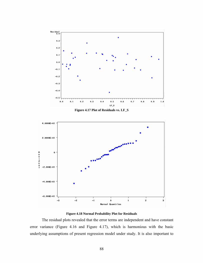
Figure 4.17 Plot of Residuals vs. LF_S
Figure 4.18 Normal Probability Plot for Residuals
The residual plots revealed that the error terms are independent and have constant
error variance (Figure 4.16 and Figure 4.17), which is harmonious with the basic
underlying assumptions of present regression model under study. It is also important to
88

analyze the residuals in order to assess their normality. This was done with the help of
normal probability plot shown in Figure 4.18. The normal probability plot does not show
departure from normality for the error terms. The tails are more or less straight and all
error terms can fall onto a straight line. Also, from these graphs we do not see any
indication for the potential outliers. The residual plots do not indicate exclusion of
important predictor variables.
4.4.3.4 Goodness of fit The goodness of the model can be tested with the lack of fit test. However, this
test requires at least one replicated observation i.e. an observation with same levels of all
predictor variables and different measured value for predicted variable, LF_P for this
case. For this reason this test could not be performed.
4.4.3.5 Test for Heteroscedasticity To test the heteroscedasticity of error terms of model, SPEC option in Proc REG
of SAS was used. The first and second moment specification results obtained are shown
in Table 4.22. High value of probability shows that the error terms are homoscedastic.
Table 4.22 Test for Heteroscedasticity
DF Chi-Square Pr > ChiSq 5 4.59 0.4677
4.4.3.6 Breusch-Pagan Test This test was used as second test for checking constancy of error variance.
Residuals (ei) obtained were squared (ei2) and regressed against the predictor variables,
LF_S and x24 to get SSR* with the help of SAS. The test statistic is obtained as, 2
2 *2BP
SSR SSEn
χ ⎛= ÷⎜⎝ ⎠
⎞⎟ … (4.11)
From SAS output we have,
SSR* = 0.0004 (ei2 regressed with LF_S and x24)
SSE = 0.71170 (LF_P regressed with LF_S and x24)
n = 35 (observations) 2
BPχ = 0.487.
89

To control a risk at 0.05, i.e. for 95 % confidence, χ2 (0.95; 3) = 7.81 [36]. Since 2
BPχ = 0.487 < 7.81 H0 is concluded, that error variance is constant. The P-value of
this test is >0.9 so the data are very consistent with constancy of error variance [36].
4.4.3.7 Multi-Collinearity Diagnostics The model built was examined for multicollinearity. No informal measures indicated
multicollinearity. These informal measures included:
• Large coefficients of simple correlation between pairs of predictor variables.
• Wide confidence intervals for predictor variables.
• Extra sum of squares associated with predictor variable changes when other
variables are added to the model.
The variance inflation factors were investigated in order to determine if there existed
any multicollinearity. The variance inflation factor for predictor variables are given in
Table 4.23.
Table 4.23 VIFs of Predictor Variables
Variable DF Variance Inflation
Intercept 1 0 LF_S 1 2.2334 x24 1 2.2334
The rule of thumb for VIF is (VIF)k < 10 and ( )
1kVIFVIF
n p= ≤
−∑ [36]. It was
found that all VIF values were less than 10 and also mean value of VIF (VIF ) was found
to be 0.14 which is less than 1. Therefore, no evidence of multicollinearity is found. After
rigorous checking model in equation 4.5 or equation 4.6 was selected as final model as it
proves to be a good fit for data. Summary of models fit is given Table 4.24.
Since polynomial models can produce unacceptable results because of their high
chances of collinearity problems, it is not recommended to use such models. Such models
yield ridiculous results even for small extrapolation and may change readily even if one
observation is removed or altered. Therefore, from Table 4.24 on the basis of maximum
coefficient of determination and adj-R2 multiple regression model (interaction model)
seems to be the best.
90

Table 4.24 Summary of Models fitted for input power measurement load and slip method load factor
Model Equation R2 adj R2
Straight line LF_P = 0.18374 + 0.9695 x LF_S 0.7488 0.7412
Polynomial LF_P = 0.31887 - 4.86*LF_S + 59*LF_S2 - 238.15*LF_S3 + 456.76*LF_S4 - 415.96*LF_S5 + 144.45*LF_S6
0.7706 0.7215
Multiple regression
LF_P = 0.14511 + 0.7786 x LF_S + 2.07 x 10⁻⁵ x S x Volt 0.7843 0.77
To visualize the modeled relationship between load factor obtained by power
measurement and slip load factor, a response surface of equation 4.5 is plotted with the
help of MATLAB®. The LF_S has limits between 0 to 1 and x24 which is a interaction
term is found to have limits between 72 and 198,000 for the collected data. Using these
limits a response surface was plotted as shown in Figure 4.19.
Figure 4.19 Response Surface for Model Fitted to Data
4.5 Model Validation As discussed earlier the data was splitted into model building data set and
validation data set or prediction data set, which was used to validate model. For
91

validation of the model MSPR criteria has been used. 10 observations were available for
validation of the model. By far the preferred method to validate a regression model is
through collection of new data. Often, however, this is neither practical nor feasible [36].
Since entire data set is not very large here to make an equal split the model validation
data split will need to be smaller than the model building data set. 80-20% split is
considered here to maintain the strength of model building data. The more the data in the
model building data set the better the model. When data are collected sequentially in
time, it is often useful to pick a point in time to divide the data. Generally the earlier data
is used for model building and later data for model validation. Use of time point to split
data set provides the opportunity to test the generalizability of the model since conditions
differ for the two data sets. The validation data set contains motors in the range of 30hp –
250hp. The model building data set has motors in range of 20hp – 250hp. can be
calculated using the model fitted. The sum of squares of difference between Yi and
over number of validation observation will give us MSPR. Detailed calculations are
shown in Table 4.25.
Y
Y
Table 4.25 Validation of Selected Model
Sr. HP S Volt LF_S LF_P (Yi) Yhat (Yi- Yhat)2 40 125 21.8 460 0.872 1.054 1.031729 0.000496 41 250 30.8 460 0.832 1.039 1.086324 0.00224 42 100 10.1 460 0.673 0.789 0.765326 0.00056 44 125 12.4 480 0.62 0.74 0.751108 0.000123 46 150 2.9 460 0.121 0.421 0.266948 0.023732 47 75 9.5 460 0.475 0.679 0.605448 0.00541 49 30 20.1 460 0.502 0.587 0.727452 0.019727 50 50 55 460 0.733 1.219 1.239787 0.000432 51 60 3.4 480 0.995 1.126 0.953616 0.029716 52 30 19.9 460 0.068 0.199 0.387634 0.035583 Total (Yi-Yhat)2 = 0.118019
Mean square error of prediction = MSPR =
*
1
2ˆ( )
*
n
ii
Y Y
n=
−∑
*
1
2ˆ( )n
ii
Y Y=
−∑ = 0.118019
92

n* = 10 = observations available for model validation
MSPR = 0.0118019
From Table 4.16, the mean square error of the model, (MSE)model = 0.02372. It can
be seen that MSPR < (MSE)model. Therefore, it can be concluded that the present model
will produce adequate results for different set of observations. The model is validated.
Since the MSPR is fairly close to MSE based on the regression fit to the model building
data set, the MSE for the selected regression model is not seriously biased and gives an
appropriate indication of the reasonable predictability of the model [36].
4.6 Summary & Conclusion
This chapter focused on analyzing collected field data statistically in order to develop
a meaningful model for prediction of power measurement load factor from slip load
factor of motor. Mainly three types of models were investigated, viz. straight line,
polynomial and multiple regression. The models are summarized in Table 4.24. The
findings are summarized below:
• Multiple regression model was found to be the best because of highest coefficient
of determination and adjusted R2as indicated in Table 4.24.
• The residuals of this model were analyzed with hat matrix leverage values (hii),
DFFITS and DFBETAS to remove outliers in the data to further refine the model.
• Breusch Pagan test conducted in section 4.4.3.6 proved constancy of error
variance.
• Thus model was tested for heteroscedasticity (constancy of error variance) and
normality of error terms.
• The model has no multicollinearity problems as has been check by variance
inflation factors VIF in section 4.4.3.7.
• The model is validated in section 4.5, proves that model can predict input power
measurement load factor from slip load with mean square prediction error
(MSPR) less than mean square error (MSE) of the model.
93

Chapter 5
5 Load Factor Discrepancies and Other Considerations
As mentioned in Chapter 1 it has been found that motors installed in the industry are
largely under-loaded. In the study carried out by X-Energy in 1998, over the nation it was
found that more than 40% of 5hp or larger motors were running below 40%. Also, in the
present study in which motors were monitored from 15 facilities, it was found as stated in
Chapter 1 that 31% of motors were loaded below 40% and 15% were loaded 40-60%.
The reasons why are motors oversized are discussed in following section.
5.1 Reasons for under-loaded motors There are several reasons for which oversized motors are such a commonplace in
the industry. Some of them are discussed here:
5.1.1 Application Need Many motors are oversized for their applications. Motors are installed in a facility
for an atypical application which requires instantaneous high power but drops down
below average for other time of the load cycle. In such cases motors with specific
controls on them would be beneficial especially ASDs might help in this case. Premium
efficiency motors may prove even worse for these kinds of applications than standard
efficiency motors [40]. Thus uncertain loads might force plant personnel to install
oversized motors.
5.1.2 Purchasing practices In many plants a motor is replaced or repaired without engineering analysis and is
often replaced with the same size, brand, and model number. Only in the case of large
motors (over approximately 250 hp) with reasonably high operating costs does an
engineering or economic analysis usually precede decisions concerning replacement of
the motor.
End-users can obtain information on motors and related equipment from manufacturers’
catalogs, trade publications, manufacturers’ representatives, distributors, contractors, and
professional organizations. It is common belief that motors under approximately 200 hp
94

and other drive power components are same though from different manufacturers and are
interchangeable. This may be true from the functional perspective; it could not be further
from the truth from an energy efficiency perspective [26]. For many customers, purchase
decisions are made based primarily on reliability, price, and availability, not on
efficiency. Consequently, energy cost saving is a factor in decisions, but not a primary
concern. Some large companies and exceptionally a smaller one have formal motor-
purchase policies that address motor efficiency; however, most do not.
5.1.3 Aversion to Downtime In many businesses, particularly in industry, shutting down equipment for
upgrading or replacement can mean losing thousands of dollars per hour in forgone
production. Such penalties may induce an understandable aversion to downtime. Because
of this, many facility managers shy away from new, unfamiliar technology that they fear
might be less reliable than the equipment they are used to. Furthermore, if a high-
efficiency substitute for a failed motor is not stocked by the distributor, in order to save
time the user is likely to buy a standard replacement or simply repair the old motor just to
put production back in place as quickly as possible. Also, if a properly sized motors fails
while in operation, the plant personnel tend to put spare motor available in shop to restore
production. If a same sized motor is not available generally it will be replaced by a higher
sized motor. Thus, availability of the motor also plays vital role.
5.1.4 Maintenance Practices Motor maintenance practices are generally limited to what is needed to keep
equipment running rather than attempting to optimize performance and save energy. Most
industrial plants and large commercial firms have full-time maintenance staff that
regularly lubricate (and often over-lubricate) motors, listen for bearing noise (a sign of
wear or misalignment), and check and tighten belts as needed [26]. Few firms do some
more sophisticated monitoring or maintenance work on motor systems. But motor loads
are hardly monitored to figure out the actual capacity needed. No maintenance analysis is
followed to analyze early life failure of motor. It is known that constant under-loaded
running of motor can substantially deteriorate its life [26]. Motors are run with out even
noticing that they are oversized.
95

5.1.5 Downsized Production In some cases, it might so happen that production volume is decreased because of
loss of business or moving the production unit to other places. Original production
requirements then are reduced, leaving a grossly oversized motor in place.
5.1.6 Allowance for load growth Many motor design professionals figure that the increase in price for a larger
motor is a small price to pay for the capability to handle higher loads if the use of the
motor changes over time. Also, sometimes while designing certain design factor is
applied to compensate for growth of production over the years of life of motor.
5.1.7 Rounding up to the next size Sometimes, because of motors manufacturing in standard steps, the designers
have to round up the size of motor to next size. If an application needs 160 hp the motor
of 200 hp is selected at that place, leading to oversized motor.
Thus, there can be many reasons why motors are under loaded in the industry.
While many oversized motors should be downsized, some should instead be equipped
with controls that enable them to operate more efficiently at partial load. Most motors are
fixed speed motors. However, adjusting the speed to match the requirements of the loads
which generally vary over time can enhance efficiency of motor system. Speed controls
can save the most energy in centrifugal machines, which include most pumps, fans and
blowers and centrifugal air-compressors. Speed control is also effective in mills, such as
the rolling mills that produce sheet metal in a steel plant, traction drives, conveyors,
machine tools, and robotics.
Oversized motor causes low operating load factor for the motor. This reduces the
efficiency of motor considerable if the motor is operating below 50% of load. Sometimes
motor may not be undersized because of its application as discussed in section 5.1.1. In
such cases speed control may give improved performance for the system. The available
options for motor speed control include multi-speed and DC motors, hydraulic couplings,
eddy current drives and electronic adjustable speed drives (ASD). Advantages,
96

limitations, cost and applications of ASDs along with their types and operating principles
are discussed here.
5.2 Adjustable Speed Drives (ASD) The primary purpose of an adjustable speed drive is to let an AC-motor run slower.
These drives allow the motor-driven machines to produce the same output as standard
counterparts but with less electrical input, often improving manufacturing quality as well.
Such drives can also enhance motor and machine life and reduce maintenance by
allowing operation at lower temperatures and smoothing machine startup and shutdown
[41]. Adjustable speed drives operate alternating current (AC) electric motors slower than
constant speed. ASDs change the characteristics of the electricity (voltage and frequency)
powering the motor so that the speed at which the motor rotates actually changes to meets
the desired machine output level. Because throttling motor output wastes energy, ASDs
can save a great deal on energy costs by increasing the overall machine operating
efficiency.
Figure 5.1 Schematic of Adjustable Speed Drive with Feedback Loop [41]
Figure 5.1 shows a typical schematic of ASD system, which has four basic
components: rectifier, DC link, inverter, and regulator. The rectifier converts line
frequency alternating current (AC) to direct current (DC). The DC link smoothes the
output of the rectifier and, the inverter generates an adjustable frequency and voltage AC
97

output to the motor. Some applications may require regulators, which help control system
output to optimize the process requirements [42].
5.2.1 Types of Adjustable Speed Drives ASDs are also commonly referred to as variable speed drives (VSDs), variable
frequency drives (VFDs), and adjustable frequency drives (AFDs). Several types of
ASDs are available; each with its own practical applications. All are similar in controlling
motor speed by varying electrical voltage and frequency. They differ in how they
accomplish AC-to-DC conversion and DC-to-AC inversion. The three most common
rectifier/inverter types are discussed below; many hybrid forms combine characteristics
of these basic types.
5.2.1.1 Current Source Inverter (CSI) A CSI actually uses the inductive characteristic of the motor to stabilize DC as it
reaches the inverter. Because the inductor has to be fairly large to keep the current source
stable, this type of electronic ASD is generally used with 100-hp and larger drives. It is
harder to tune in the field because it cannot operate without connection to the motor [41].
5.2.1.2 Voltage Source Inverter (VSI) The VSI is sometimes called a variable voltage inverter (VVI) or six-step inverter.
It uses a capacitor before the inverter to store energy from the rectifier and stabilize the
voltage entering the inverter. It is used in low to medium power applications, generally
up to a few hundred horsepower [42].
5.2.1.3 Pulse-Width Modulated Inverter (PWM) The PWM inverter develops the voltage output by chopping pulses of varying
widths to synthesize the desired waveform. PWM drives use complex software
algorithms to determine timing, duration, and frequency of the voltage pulses delivered to
the motor. Each manufacturer employs its own algorithms, causing significant differences
in motor performance and life. This is presently the most common ASD type for up to
400-hp motor sizes. These drives are well suited for motors up to 100,000 hp, but above
1,000 hp, electronic components and inverter controls are more complex [42]. Discussed
are the most common types of ASDs. Those not included in discussion are load
commutated inverter, cycloconverter and vector control ASDs.
98

5.2.2 Benefits of Using ASDs • Energy savings can be very significant in many situations, depending on the
existing system design, installed equipment and motor load requirements.
• Speed reduction may extend the life of a machine and motor due to reduced
stresses and fewer revolutions.
• ASDs start motors gradually, reducing stress on drive components such as belts.
This gradual start reduces maintenance on these components and the effect of
fluctuating voltage due to the sudden start of a large motor.
• A single ASD can control several motors at once. All the motors connected to the
drive will operate at the same speed.
• Some ASDs can operate motors at speeds greater than their original design speed.
• PWM ASDs can significantly improve power factor.
• Some ASDs provide power regeneration when the motor slows down.
• Speed control can be accomplished in many ways based on load requirements.
• Some speed control sensors include rpm, temperature, pressure, flow, and power.
5.2.3 Drawbacks of ASDs • If the motor operates at or near full speed most of the time, adding an ASD will
increase overall energy consumption, due to energy losses in the drive.
• ASDs may increase motor heating, especially at slower speed. Many motors rely
on internal cooling fans attached to the motor shaft to remove internal heat. At
slower speeds, the heat generated internally may not decrease in proportion to the
fan's cooling capacity so additional cooling may be required.
• Some ASDs can produce electrical interference that harms other electronic
equipment at the facility, so electrical isolation equipment may be required.
• The additional electronics associated with an ASD add to the maintenance and
repair complexity of the drive system.
• An ASD may be less efficient than a two-speed motor in situations where speeds
between high and low are not required.
• Each ASD application needs to be carefully considered and engineered for proper
installation and compatibility.
99

5.2.4 Applications of ASDs ASDs are best suited for modifying the speed of centrifugal machines to provide the
exact flow required by the system. Fan, pumps, blowers and compressors come under this
category. In general following are good situations for variable speed flow control [42].
• The applications are fixed at a flow rate higher than that required by the load.
• The application is variable flow, where variation is provided by throttling and
where the majority of operation is below design flow.
• The applications use flow diversion or bypassing via pressure reducing valve.
• The applications are greatly oversized for the flow required.
• The applications have long distribution networks.
• The applications are single stage rather than multiply staged pumps or fans.
A typical system efficiency curve having ASD installed is shown in Figure 5.2.
Figure 5.2 ASD, Motor and System Efficiency vs. Partial Load [42]
It can be seen that there will be always more energy consumption if the motor
keeps on operating at rated load. However, if motor comes down below rated load even
for small amount of time, the amount of savings that are produced justifies the
installation of ASD.
100

5.3 Discrepancies in Load Factors As noted in Chapter 3, large discrepancies exist in the loads obtained by different
methods of estimating load factor for recorded motors. Out of four methods used for
estimation of load, the load obtained by input power measurement is compared with each
of the method below.
5.3.1 Slip Method The load comparison graph for slip method compared with load factors obtained
with input power measurement is reproduced in Figure 5.2 below.
Comparision of Load factor obtained by slip and power measurement methods
0.000
0.200
0.400
0.600
0.800
1.000
1.200
Motors
Load
Fac
tor
Load By Slip Method Load by Pow er Measurement
Figure 5.3 Discrepancy in Load Factors Obtained by Slip Method and I/P Power measurement Method
As can be seen in the graph, the load obtained by power measurement method is
always on higher side as compared with the load factor obtained by slip method. This is
true at all points except a few where the load obtained by power measurement is actually
less than the load obtained by the simple slip method. A possible explanation of this is
given in following sections. The average of load factor discrepancies obtained at each
horsepower motor is plotted against horse power of motor in Figure 5.4.
101

Discrepancy Comaprison
0.000.050.100.150.200.250.30
20 25 30 40 50 60 75 100
125
150
200
250
HP
Diff
eren
ce in
Loa
d Fa
ctor
s
Figure 5.4 Load factor discrepancy for slip method vs. Motor HP
As we can see there is no specific pattern in the differences obtained with respect
to horsepower. The differences reduce till the size increases to 40-50 hp but again start to
increase once the size further starts increasing. This may be due to high losses associated
with low and high horsepower motors as discussed later.
5.3.2 Voltage Corrected Slip Method A graph showing comparison of load factors obtained by voltage corrected slip
method with load factors calculated using input power measurement method is shown in
Figure 5.5. This method is a modification of simple slip method in that, a correction of
voltage is applied to the previous method in order to compensate for the slip because of
voltage unbalance. This method shows more or less similar behavior as simple method
itself.
Comparision of Load factor obtained by V-corrected slip and power measurement methods
0.000
0.200
0.400
0.600
0.800
1.000
1.200
1.400
Mot ors
Load by Pow er Measurement Voltage Corrected Slip (B)
Figure 5.5 Discrepancies in Load Factors obtained by Power Measurement and Voltage Corrected Slip
102

With this method also, the load factor obtained, most of the time, is less than the
power measurement load factor as shown in Figure 5.6. The differences in load factor
obtained when plotted against the horsepower of motor shows that load factor differences
for the horsepower ranges 40- 50 hp is negative. The load factor differences for this
category had lowest values in slip method.
Discrepancy Comaprison
-0.10
-0.05
0.00
0.05
0.10
0.15
0.20
0.25
20 25 30 40 50 60 75 100
125
150
200
250
HP
Diff
eren
ce in
Loa
d Fa
ctor
s
Figure 5.6 Load factor discrepancy for voltage corrected slip method vs. Motor HP
5.3.3 Current Voltage Method
Comparision of Load factor obtained by slip and power measurement methods
0.000
0.200
0.400
0.600
0.800
1.000
1.200
1.400
1.600
Motors
Load
Fac
tor
Load by Pow er Measurement V-I (D)
Figure 5.7 Discrepancies in Load Factors obtained by Power Measurement and Current Voltage Method
103

The load factors obtained by this method exhibit different behavior than both
methods discussed above. In this case the load factors are almost equally divided into
higher or lower regions as compared to the input power measurement load factor. The
graph shown in Figure 5.7 illustrates this fact.
Differences in the load factors obtained are plotted against horse power of motors
in Figure 5.8. The graph shows that, the considered method obtains very low load factors
for motors in horse power category 40-50 hp. Also, the differences are distributed in
positive and negative regions and go on increasing as the horse power increases.
Discrepancy Comaprison
-0.50
-0.40
-0.30
-0.20
-0.10
0.00
0.10
0.20
20 25 30 40 50 60 75 100
125
150
200
250
HP
Diff
eren
ce in
Loa
d Fa
ctor
s
Figure 5.8 Load factor Discrepancy for Current Voltage Method vs. Motor HP
To get a good idea of how load factors differences behave with respect to horse
power of motors a collective graph of Figures 5.4, 5.6, 5.8 would be helpful. Such a
graph is shown in Figure 5.9. As we can see, except for some categories of HPs the
voltage corrected slip method acts towards reducing the difference between load factors
obtained by slip method and input power measurement method. For HPs 40 and 50 we
get least differences by slip method and voltage corrected slip method while for current
voltage method, the difference in this category is the highest.
104

Discrepancy Comaprison
-0.50
-0.40
-0.30
-0.20
-0.10
0.00
0.10
0.20
0.30
0.40
20 25 30 40 50 60 75 100
125
150
200
250
HP
Diff
eren
ce in
Loa
d Fa
ctor
s
Slip Load Voltage Corrected Slip Load Voltage Current Load
Figure 5.9 Load Factor Discrepancies vs. HP of Motors
5.4 Reasons for Load Factor Discrepancies The load factors of recorded motors are evaluated to find that it is relatively very easy
to evaluate load factor for a motor with slip method, as we just need to measure operating
speed of that motor. However, the actual load varies from the slip load values because of
following:
1. Rated speed on nameplate is rounded off to nearest multiple of 5
2. Motor is rewound number of times in its lifetime and its rated speed changes
3. Error in the measurement of operating speed
Also as specified in Table 2.3 in Chapter 2, NEMA has allowed certain tolerance
limit for specification of the rated parameters of speed, voltage and current on the
nameplate of motor. This may account for error in the loads calculated using these values.
Fairly accurate load factor of motor can be found out using input power measurement
method. Inaccuracies exist with this method also due to inaccuracy in estimating
operating efficiency of motor. Nevertheless, it is pretty accurate method to estimate load
factor of an in-situ motor. The limitations of the slip method are that it does not recognize
actual current losses which vary at loaded and no-load conditions, and the calculations
rely upon the value indicated on the motor nameplate for speed (rpm) at full load which is
an average for groups of similar motors tested by the manufacturer.
105

One more reason for slip load not matching with input power measurement load
may be that, while estimating it is assumed that slip of motor is directly proportional to
the load on the motor. This is because the load factor falls in a region near to the rated
speed on the torque-speed curve. The torque-speed curve though not exactly is almost
linear in this region. For low values of slip, this happens to be true but for larger values it
may deviate slightly from the straight line assumption.
Developed torque is given by, Equation. 5.1
( )
2 2
222
2
'( )
' '
Th
d
Ths Th
RVsT
RR X Xs
ω=
⎡ ⎤⎛ ⎞+ + +⎜ ⎟⎢ ⎥⎝ ⎠⎣ ⎦
… (5.1)
Where,
VTh = Voltage of Thevenin’s equivalent circuit, volts
RTh = Thevenin’s equivalent circuit resistance, Ohm
XTh = Thevenin’s equivalent circuit reactance, Ohm
ωs = Synchronous angular speed of motor, rad/sec
s = %Rated slip of motor, fraction
R2’ = Stator equivalent resistance, Ohm
X2’ = Stator equivalent reactance, Ohm
For small slip values the curve can be assumed as straight line on torque vs. speed curve, 2
. 2 'Th
ds
V sTRω
≈ … (5.2)
If this underlying assumption is not satisfied, the load factor value will tend to be
different than obtained by input power measurement method.
5.5 MATLAB GUI for torque-speed curve generation To explain the discrepancy in the obtained slip load and load factor obtained by
power measurement method a MATLAB graphical user interface (GUI) is developed. In
the MATLAB program the parameters of the equivalent circuit of a motor can be entered
on the circuit diagram. The program draws the Thevenin's equivalent circuit [32].
Performance characteristics are then obtained for the specified slip and the torque slip
curve is plotted on the screen. The analysis can be repeated for different slips. The GUI
106

can be used to estimate parameters for different motors and thus helpful in getting
operating characteristics of a particular motor. The input screen for the graphical user
interface is shown in Figure 5.10. User can input data on motor nameplate data in the
frame motor nameplate data.
Figure 5.10 Input Screen for MATLAB GUI to Calculate Performance of Induction Motor
The equivalent circuit parameters can be entered into the edit boxes below
equivalent circuit parameters. The program draws equivalent circuit as shown in Figure
5.11 with respective label.
Figure 5.11 Equivalent Circuit Produced by MATLAB GUI
107

Information about the program is given when ‘Info’ button is clicked on the GUI.
It summarizes the formulae used in calculating the performance characteristics for motor
being evaluated. The info screen is shown in Figure 5.12.
Figure 5.12 Information Screen – Formulae Used for Calculation of Performance for Motor
When ‘Solve’ button is hit the program analyzes the equivalent circuit of the
motor with given parameters. It draws a Thevenin’s equivalent circuit for motor at the
specified slip in the input box. A torque vs. rotor speed curve also plotted as shown in
output screen of the program in Figure 5.13. The program estimates the losses of the
motor for given equivalent circuit parameters of motor. In the graph shown in Figure 5.13
the two vertical lines mark the operating and rated slip of motor.
108

Figure 5.13 Output Generated by Designed GUI and Operating Characteristics of Motor
5.6 Validation of Statistical Model Built Considering Losses in Motor The model built for prediction of power measurement load factor was validated
statistically in Chapter 4. Efforts have been made here to validate the model based on
electrical parameters, taking into consideration, the losses incurred in motor when it is
operating. The losses that occur in motor include stator and rotor copper losses, core
losses, rotational or friction and windage losses and stray losses. While copper losses and
core losses can be calculated from the equivalent circuit parameters of motor friction and
windage losses depend on system and stray load losses cannot be accounted for.
Generally as a rule of thumb stray load losses are assumed to be 1.5 % of motor input (as
suggested by IEC standard) [51]. Following motor was considered for validation of
model. Only one motor has been used here as it is very difficult to get data for equivalent
109

circuit parameters of motors. Also, it is very time consuming and involve rigorous
experimentation for calculation of the same. For this only one motor has been considered
here.
Nameplate Data
Size 5 HP
Voltage 230 Volts
RPM 1740 RPM
Frequency 60 Hz
s 0.033
S 60 RPM
Equivalent circuit data
R1 0.6 ohm
X1 0.8 ohm
R2 0.4 ohm
X2 0.5 ohm
Rms 400 ohm
Xms 20 ohm
From the statistical model proposed in equation 4.6,
LF_P = 0.14511 + 0.77860*LF_S + 0.00002071*S*Volt
At rated conditions,
LF_S = 1.00, S = 60 , Volt = 230,
LF_P = 1.20 … (5.3)
The equivalent circuit with parameters shown in Figure 5.14 is analyzed using
conventional analysis approach.
400
Ir
R2 (1-s)/s
0.6 0.8 0.4 0.5
Is
20132.79 @ 0o
400
Ir
R2 (1-s)/s
0.6 0.8 0.4 0.5
Is
20132.79 @ 0o
Figure 5.14 Per Phase Equivalent Circuit for the Motor
By nodal analysis,
IS = 12.3 amps L- 33.9o
IR = 10.1 amps L- 4.3o
Vm = 121.3 L-1.91o
110

The losses are calculated for all the 3-phases as,
Stator Cu Loss = PS = 3 IS2R1 = 3(12.3)2(0.6) = 271 W
Rotor Cu Loss = PR =3 IR2R2 = 3(10.1)2(0.4) = 122 W
Pcore = 3 Vm2 / Rms
= 3 (121.3)2 / 400 = 110 W
Friction and windage losses depend on motor. It usually depends on the components like
bearings and rotational components. A value of 210 W is reasonable to assume for the
kind of motor under consideration.
To determine stray losses IEC standard graph was used which is shown in Figure 5.15.
Figure 5.15 Determination of Stray Losses, IEC 61972 [51]
For 5 hp (3.73kW), the graph shows stray load losses of 2.6% of input power Pin.
The mechanical output power of motor is the horsepower rating on nameplate. For 5 hp
motor, mechanical O/P Power = 5 x 746 = 3,730 W
The stray load losses are assumed to be 115 W for time being, later these are
checked with input power calculated in order to check of they are within limits. The input
power can be calculated as [32],
Pin = Mechanical Power + Ps + PR + Pcore + PF&W + Pstray
Pin = 3,730 + 271 + 122 + 110 + 210 + 115
Pin = 4,558 W
To check value of stray load losses, Pstray = 2.6/100 x 4,558 = 118.5 W > 115 W.
111

To estimate rated input power,
Pir = Mech. O/P Power 3,370 4,1350.902motormaster
Wη
= =
Load factor can be calculated as,
LF = 4,558 1.1034,135
= … (5.4)
Comparing equation 5.3 and equation 5.4
% error = 0 1.20 1.103 8%1.20
x xx− −
= =
∴error2 = 0.0064 < MSEmodel (0.02372) as given in Table 4.11 (a). It can be said
that the model has acceptable behavior from electrical point of view as well from the
above verification. Figure 5.16 shows output for 5 hp motor from developed MATLAB®
GUI.
Figure 5.16 Operating Characteristics and Torque-Speed Curve for 5 hp motor
The output shows Thevenin’s equivalent circuit drawn for the 5 hp motor. Also it
can be seen from output in Figure 5.16 that values of currents Is, IR match with those
112

obtained by calculation. The values for copper losses in stator and rotor and also the
value of core losses match with those obtained by manual calculation.
5.7 Summary & Conclusion
• Motors are under loaded for a number of reasons in industry as has been discussed
in 5.1. One of major effective method to handle fluctuating loads on motor is
ASD. It is discussed along with advantages and disadvantages in 5.2. If a motor is
oversized because of application it is installed for, ASD can be helpful to improve
system performance.
• The load factors obtained by slip method, voltage corrected slip method and
current-voltage method are compared with load factor calculated by input power
measurement method in section 5.3. The slip method and voltage corrected slip
method most of the times produced load factor less than that by power
measurement method. This was not true for current voltage method.
• The discrepancy for slip methods was least for motors ranging in 30-50 hp. For
current-voltage method this discrepancy was negative most for this category of
motor hp. Reasons for these discrepancies are discussed in section 5.4.
• Torque-speed curve can be generated for motor with known equivalent circuit
parameters using MATLAB® graphical user interface in section 5.5. The GUI
also helps in determining losses in the motor, which can be used to find actual
load factor of motor.
• For example a 5 hp motor is considered. Model developed in Chapter 4 gives
input power measurement load factor at 100 % slip as, 1.2. The load factor
obtained from electrical principles is 1.103 which gives 8% deviation from the
model result. The squared deviation is less than MSE of the model. In future more
motors should be used to validate model from electrical principle using same
approach.
113

Chapter 6
6 Conclusion and Future Work
6.1 Conclusion In this research motor data was collected from 15 facilities which were audited for
energy assessment. This data was analyzed with the purpose of developing a model to
obtain actual load factor of motor from load factor obtained by simple slip method. The
author also performed an overview of relationships between two other methods of load
factor measurement and actual load factor, viz. voltage corrected slip method and line
current method. However, these relationships were not emphasized. The relationship
obtained between voltage corrected load factor and input power measurement load factor
is,
LFI/P = 0.8893*LFslip-volt + 0.2104
Where,
LFslip-volt = Load factor obtained by voltage corrected slip method
LFI/P = Load factor obtained by input power measurement method
For load factors obtained by line current method and input power measurement
method it was found that there existed no simple relationship. Investigation was not
carried out further to analyze that data. The model of major interest was the relationship
between load factor obtained by slip method and load factor obtained by input power
measurement method. The model is presented by following equation,
LFI/P = 0.14511 + 0.7756*LFslip + 0.0002071*S*Volt
Where,
LFI/P = Load factor obtained by input power measurement method
LFslip = Load factor obtained by slip method
S = Measure slip, RPM = Synchronous speed – Measured speed.
Volt = Nameplate voltage rating of motor being investigated.
This model showed coefficient of determination, R2 as 0.7843 and adjusted R2 as
0.77 which is fairly high for this kind of model. The model was successfully validated
with data from 10 motors. The value of mean square prediction error (MSPR) was fairly
below MSE of the model which shows fair validity of the model. The model was also
114

validated electrically with one motor for which equivalent circuit parameters were
known. The losses were calculated and load factors obtained showed 8% error.
The model developed will be extremely helpful to the industrial end users who
can not devote required time and cost that goes into power measurement and efficiency
estimation. The model will also provide safe and easy way to measure load on three
phase induction motors with which the load can be estimated fairly accurately and based
on which certain important decisions such as how the motor should be optimally sized to
achieve maximum energy efficiency can be based. The model developed clearly has
following advantages:
• Easy technique for load estimation, one has to just use stroboscope to measure the
operating speed.
• The load measurement will not have safety problem as no connections involved
around high voltage areas.
• The load measurement will be extremely less time consuming.
• The cost of expensive equipment and the labor that goes for load estimation will
be almost eliminated
• Lastly, with all the above advantages the load estimated will be in fairly accurate
range on which responsible decisions could be based regarding motor sizes.
6.2 Future Work When unequal phase voltages are applied to a 3-phase induction motor unbalanced
currents in stator winding result. A small percentage of voltage unbalance will result in
large unbalance of currents and consequently, the temperature of motor will rise at a
particular operating load. This reduces performance of the motor. To take this into
account the horsepower of motor should be multiplied by a factor that is obtained from
graph given in Figure 6.1. Thus voltage unbalance wastes energy and leads to high losses
in induction motor. A voltage unbalance of 2 % may lead to 25 % increase in losses [26].
It is desired that these derating factors should be taken into account when measurements
are done for calculating load factors. This may be done in a future study if undertaken.
115

Figure 6.1 Derating Factor Due to Unbalance in Voltage
Also, it is important to find out losses that occur in the induction motor. This is
possible for a motor if equivalent circuit parameters are known for that motor. In the
future study observation for motors should be carried out for which equivalent circuit
parameters are known.
If equivalent circuit parameters are known for the motors, it will enable us to
determine operating efficiency of motor more accurately which can then be used in
determination of input power measurement load factor. This will lead to increased
accuracy of the model. To summarize following future work is suggested.
• Study and analyze effect of voltage unbalance on motor losses, efficiency and
hence load factor of the motor. Appropriate amendments can be made in the
model to accurately estimate the motor load.
• Motors for which equivalent circuit parameters are known can be tested to have a
better accuracy in efficiency and load estimation for motor.
• More of the similar data can be collected to enhance model developed. Data can
be grouped according to the category of their applications e.g. compressors or
pumps.
116

References [ 1 ] Beaty H., Kirtley J. Jr., “Electric Motor Handbook”, McGraw Hill Book
Company, 1998.
[ 2 ] Brender, D., “Calculating motor system energy savings”, Strategic Planning for
Energy and the Environment Journal, Vol 16, no.2, p 72-78, Fall1996.
[ 3 ] Bush, D., Maestas, J., “Effective Load Management Planning – A Case Study”,
Energy Engineering, Vol. 99, No. 3, 2002.
[ 4 ] Cogdell, J., “Foundations of Electrical Engineering”, Prentice Hall, Second
Edition, 1996.
[ 5 ] Cole, R.; Thome, T., “Motors matched to load profiles lead to high-efficiency
service”, Pulp & Paper, Vol 69, no.8, 6pp., Aug 1995.
[ 6 ] Consulting- Specifying Engineer Magazine, “Weyerhaeuser Policy Calls for
Premium-Efficiency Motors and Transformers”, Reed Business Publications, Jan
2003.
[ 7 ] Cowern, E., “Effectively applying premium efficiency motors”, Electrical
construction and maintenance, v 94, no 3, 4pp, March 1995.
[ 8 ] EASA Reliable Solutions Today, “A Guide to AC Motor Repair and
Replacement”, http://easa.com/indus/ac_gd199.pdf, Electrical Apparatus Service
Association, 1999.
[ 9 ] EASA Reliable Solutions Today, “Understanding Energy Efficient Motors”,
Electrical Apparatus Service Association, http://easa.com/indus/ee_399.pdf, 1999.
[ 10 ] Fairford Electronics, “The Fixed-Speed Induction Motor Energy Optimizer–
Science Or Snake Oil?”, <Website>,
www.ienergyideas.com/pdfs/SD00014x1Snakeoil.pdf, 2003.
[ 11 ] Grantham, C., Tabatabaei-Yazdi, H., “A Novel Power Electronic Machineless
Dynamometer for Load Testing and Efficiency Measurement of Three-Phase
Induction Motors", Proceedings of The Third International Power Electronics and
Motion Control Conference, IPEMC2000; 15-18 Aug., 2000, Beijing, China,
IEEE Catalogue No. 00EX435 , Vol. 1, pp 564 - 569.
[ 12 ] Hardware User’s Manual, DM II Pro Datalogger, Amprobe™.
117

[ 13 ] Hirzel, J., “Impact of rewinding on motor efficiency”, Annual Pulp and Paper
Industry Technical Conference, available from IEEE service center c1985-, June
20-24, 1994.
[ 14 ] Jordan, H., “Energy Efficient Electric Motors and Their Application”, Van
Nostrand Reinhold Company, 1983.
[ 15 ] Lincoln Electric Motor Division, “How Accurate is AC Motor Energy Auditing”,
Lincoln Electric Company, http://www.lincolnmotors.com/pdf/D11T.pdf, June
1997.
[ 16 ] Lobdovsky, K., “Motor Efficiency Management”, Energy Engineering, Vol. 91,
No.2, 1994.
[ 17 ] Lung, R., et. al., “Industrial Motor System Optimization Projects in the US: An
Impact Study”, ACEEE, Proceedings of the ACEEE Summer Study on Energy
Efficiency in Industry, Washington DC, 2003.
[ 18 ] Mate, A., “Energy Analysis and Diagnostics in Wood Manufacturing Industry”
Master's Thesis, West Virginia University, 2002.
[ 19 ] McCoy, G.; Rooks, J.; Tutterow, V., “MotorMaster+: An energy-efficient motor
selection and energy management tool for the pulp and paper industry”, Annual
Pulp and Paper Industry Technical Conference, available from IEEE service
center, c1985-, June 16-20,1997.
[ 20 ] Mecker, S., “How loads affect efficiency of motors”, Electrical construction and
maintenance, Vol 93, no.8, p33-35, Aug 1994.
[ 21 ] Mecker, S., “What makes a motor more efficient?” Electrical construction and
maintenance, volume 93,no.5, 3p, May 1994.
[ 22 ] Pacific Energy Center Factsheet, “Efficiency Improvements of AC Electric
Motors”, Pacific Gas Electric Company, May 1997, <Website>,
http://www.pge.com/003_save_energy/003c_edu_train/pec/info_resource/pdf/acm
otors.pdf
[ 23 ] Sanchez, I.; Pillay, P, “Sensitivity analysis of induction motor parameters”,
Southeastcon '94 : creative technology transfer : a global affair, p 50-54 Miami,
FL, April 10-13,1994
118

[ 24 ] Selvaraj, R., “Plant-Wide Energy Assessment using a Systems Approach” Master's
Thesis, West Virginia University, 2003.
[ 25 ] Spee, R.; Wallace, A., “Comparative evaluation of power-factor improvement
techniques for squirrel-cage induction motors”, IEEE Conference, p 12-17,
Seattle, WA. Oct 7-12, 1990.
[ 26 ] Steven N., et al., “Energy-efficient motor systems: a handbook on technology,
program, and policy opportunities”, ACEEE Publications, 2002.
[ 27 ] United States Department of Energy, Motor Challenge Program, “Determining
Electric Motor Load and Efficiency” (FACT SHEET), 2001.
[ 28 ] Vaughen, D., Kota, S., University of Michigan, website for course ME 350,
<Website>, http://www.engin.umich.edu/labs/csdl/ME350/motors/ac/induction/3-
phase/
[ 29 ] Wallace, A.; et. al., “Effects of voltage and winding abnormalities on the
measured performance of induction motors”, IEEE Conference, p 196-200 New
Orleans, LA, Oct 5-9 1997
[ 30 ] Wallace, A., et. al. “Measured effects of under-voltage, over-voltage and
unbalanced voltage on the efficiency and power factor of induction motors over
wide ranges of load”, International Conference on Electrical Machines and
Drives (proceedings), p 258-262, Cambridge, UK, Sep 1997.
[ 31 ] Website, “Energy Facts”, Http://www.solarenergy.org, Solar Energy Internatinal,
Renewable Energy and Sustainable Future.
[ 32 ] Wildi, T., “Electrical Power Technology”, John Wiley & Sons, 1981.
[ 33 ] Will, F. C., “Factors That Affect Your Plant Power Bill”, Annual Paper and Pulp
Conference, IEEE 1993 Annual Textile, Fiber and Film Industry Technical
Conference, Crowne Plaza Ravinia, Atlanta, Georgia May 4-6, 1993.
[ 34 ] Scheihing, P., et. al. “United States Industrial Motor-Driven Systems Market
Assessment: Charting a Roadmap to Energy Savings for Industry”, Paper
presented at the International Workshop on Industrial Energy Efficiency Policies:
Understanding Success and Failure, Utrecht, The Netherlands, June 10-12, 1998.
[ 35 ] [35] Ashram, H., ‘Statistical data analysis: Prove it with data’, Manchester
Metropolitan University website, 1996,
119

http://obelia.jde.aca.mmu.ac.uk/resdesgn/arsham/opre330.htm [ 36 ] [36]Neter, J., Kutner M., et. al. “Applied Linear Regression Models”, The McGraW
Hills Companies, 3rd edition, 1996.
[ 37 ] [37]Neter, J., et. al. “Applied Linear Regression Models—Table of Percentiles of χ2 –
Distribution”, The McGraw Hills Companies, 1996, pp.688.
[ 38 ] [38]Der, G., Everitt, B., “A Handbook of Statistical Analyses using SAS”, Chapman
& Hall CRC, 2nd edition, 2002
[ 39 ] [39]Delwiche, L., Slaughter, S., “The Little SAS Book: A Primer”, BBU Press, 3rd
edition, 2003.
[ 40 ] [40]Jordan, H., “Energy Efficient Electric Motors and Their Application”, Van
Nostrand Reinhold Company, 1983.
[ 41 ] [41]Application Note, “Efficiency Opportunities with Adjustable Speed Drives”,
Pacific Gas and Electric Company, May 1997, <Website>,
http://www.pge.com/003_save_energy/003c_edu_train/pec/info_resource/pdf/SP
EEDRIV.PDF
[ 42 ] [42]Platts Research and Consulting, “Motors: Adjustable Speed Drives”,, a Division
of The McGraw-Hill Companies, Inc., 2004.
[ 43 ] [43]Hanselman, D., Littlefield, B., “Mastering MATLAB: A Comprehensive Tutorial
and Reference”, Prentice Hall, 1996.
[ 44 ] [44]Floyd, T., “Electrical Circuits Fundamentals”, Prentice Hall, 3rd edition, 1995
[ 45 ] [45]Taber, M., Silgalis, E., “Electric Circuit Analysis”, Houghton Mifflin Company,
Boston, 1980.
[ 46 ] [46]Ong, C., “Dynamic Simulation of Electric Machinery: Using
MATLAB/Simulink”, Prentice Hall, 1998
[ 47 ] Yoshino, H., Kurata, Y., “Energy Saving Induction Motors”, Mitsubishi Electric
Advance, Technical Reports, 2000, <Website>,
http://global.mitsubishielectric.com/pdf/advance/vol90/vol90_tr6.pdf
[ 48 ] Famouri, P., Wang, J., “Loss Minimization of a DC Motor Drive”, Electric
Machines and Power Systems, 25:525-537, 1997.
[ 49 ] Angelo, C., et. al. “ Loss Minimization in DC Motor Drives”, IEEE International
Electric Machines and Drives Conference, Seattle, Washington, May 9-12, 1999.
120

[ 50 ] Famouri, P., Cathey, J., “Loss Minimization Control of an Induction Motor
Drive”, IEEE Transactions on Industry Applications, Vol. 27 no.1, 1991
[ 51 ] IEC Std 61972:1998: Method for determining losses and efficiency of three-
phase, cage induction motors.
[ 52 ] Hsu, J., et.al. “Comparison of Induction Motor Field Efficiency Evaluation
Methods”, IEEE Transactions on Industry Applications, Vol 34, no.1,
January/February, 1998.
[ 53 ] Power Systems Engineering P.S. website, http://www.powerstudies.com/content/resources/Diane%20Power%20Factor.pdf
[ 54 ] Hatanaka, T., “Supermizer- Energy Saving System for 3-phase AC Induction
Motors”, Proceedings of 1995 International Conference on Power Electronics and
Drive Systems; Singapore, 21-24 February, 1995.
121

APPENDICES
122

APPENDIX I
Figure A-1 Field Data Collection Template
123

APPENDIX II The data measured and recorded with Amprobe TM is presented in this Appendix. The average values of voltage and current are calculated from the RMS values of phase voltages and RMS values of line currents respectively. The values given for each motor are average values for the time period it was monitored. One observation for each of the values was logged each 5 seconds in AmprobeTM in the time period during which it was coupled with motor. Table I-1 Summary of data obtained in energy audits using AmprobeTM
Power Average RMS Voltage RMS Current No Size
(HP) kW (kW) (kVAR) (kVA)
PF V (Volts) I (Amp) VAB (V) VBC (V) VCA (V) IA (A) IB (A) IC (A)
1 60 44.76 19 12 22 0.84 449 24.9 449 449 449 25 25 252 25 18.65 17 3 17 0.98 466 18.2 466 466 466 18 18 183 125 93.25 15 13 20 0.74 330 73.6 266 265 460 74 74 73*4 75 55.95 35 -71 79 0.45 456 87.0 456 455 456 87 88 865 200 149.2 88 -11 88 0.99 454 187.0 453 454 454 188 188 1846 200 149.2 88 -11 88 0.99 454 187.0 452 452 453 209 226 219*7 200 149.2 28 155 157 0.18 452 218.0 452 453 453 134 121 1378 200 149.2 121 -60 139 0.91 477 171 477 476 478 167 176 1709 150 111.9 14 45 47 0.29 488 56 487 489 489 56 55 5910 40 29.84 27 17 32 0.85 481 38 481 482 481 38 39 3811 20 14.92 7 8 11 0.62 469 12.9 469 467 471 14 12 1312 150 111.9 17 71 73 0.23 470 86.4 471 468 470 91 88 8013 150 111.9 23 66 44 0.51 473 54.0 474 473 471 54 56 5214 25 18.65 15 16 22 0.70 466 28 - 465 468 28 27 2815 75 55.95 68 -37 78 0.88 492 91 491 492 493 92 93 9016 75 55.95 71 -32 77 0.91 494 91 494 494 493 90 90 92
124

Power Average RMS Voltage RMS Current No Size
(HP) kW (kW) (kVAR) (kVA)
PF V (Volts) I (Amp) VAB (V) VBC (V) VCA (V) IA (A) IB (A) IC (A)
17 200 149.2 64 6 64 1.00 489 171 490 488 489 149 182 18318 150 111.9 23 47 53 0.44 478 63 479 477 477 65 60 6319 150 111.9 80 53 96 0.82 475 114 477 474 475 118 110 11620 200 149.2 31 -16 38 0.90 473 78 473 472 475 78 77 7821 200 149.2 57 -95 111 0.52 468 231 467 467 469 227 230 23622 60 44.76 34 -7 35 0.96 474 43 473 474 475 44 42 4323 30 22.38 7 17 19 0.39 476 39 477 477 476 39 38 024 20 14.92 2 7 7 0.30 481 9.0 483 482 479 9 9 825 20 14.92 14 9 16 0.85 479 19.6 482 479 476 19 21 1926 30 22.38 15 12 19 0.76 233 48 - 234 233 52 50 4227 30 22.38 16 6 17 0.92 229 43.1 231 225 231 45 43 4128 25 18.65 12 11 16 0.75 234 40.4 232 234 235 41 39 4129 25 18.65 13 11 17 0.77 234 42.1 232 235 234 40 43 4330 75 55.95 39 28 48 0.81 472 59.6 471 471 475 59 57 6231 75 55.95 67 45 81 0.83 473 97.3 471 476 471 96 92 104*32 100 74.6 30 29 42 0.71 474 52.1 477 473 473 50 55 51*33 40 29.84 24 14 28 0.87 232 68.2 233 233 231 71 69 6534 20 14.92 2 6 7 0.35 487 10 487 488 487 7 11 1135 50 37.3 34 18 38 0.88 484 46 484 485 484 47 44 4836 50 37.3 8 10 13 0.61 485 16 485 486 485 16 14 1737 150 111.9 2 -2 3 0.60 481 147 481 482 481 148 146 14638 25 18.65 19 15 24 0.78 483 28 484 483 483 28 29 2939 125 93.25 29 91 98 0.28 457 124.5 456 455 460 127 121 126
125

Power Average RMS Voltage RMS Current No Size
(HP) kW (kW) (kVAR) (kVA)
PF V (Volts) I (Amp) VAB (V) VBC (V) VCA (V) IA (A) IB (A) IC (A)
40 40 29.84 2 1 2 0.79 231 156.2 232 232 229 156 161 15141 125 93.25 107 63 124 0.86 465 154.2 468 464 464 159 153 15142 250 186.5 216 66 226 0.96 463 273.4 466 462 462 263 278 27943 100 74.6 62 -24 68 0.93 451 87.5 451 452 450 89 88 86*44 200 149.2 61 -114 130 0.47 469 139.7 470 469 468 137 143 13945 125 93.25 74 45 87 0.86 455 110.5 455 453 456 112 109 110*46 150 111.9 86 131 157 0.55 458 170.7 459 459 456 171 169 17247 150 111.9 31 8 32 0.97 466 63.3 464 467 468 68 60 6148 75 55.95 43 -28 51 0.84 466 59.9 468 467 464 64 50 65*49 150 111.9 2 13 13 0.17 465 95 465 465 466 86 100 9850 50 37.3 49 34 60 0.82 497 69.5 498 494 500 71 67 7151 30 22.38 5 12 13 0.37 468 16.1 472 466 467 17 16 1552 60 44.76 3 -1 3 0.98 470 67.5 470 474 467 69 71 62
126

APPENDIX III The data collected in the field from the motors that were monitored is presented here. Empty spaces represent where the data could not be recorded due to difficulties in obtaining data. This data was collected in the data sheet that has been presented in the Appendix I. The speed was measured using a digital stroboscope. Other observations were obtained from the nameplate of the motor or with discussion with plant personnel. Table III-1 Data collected from 15 facilities in data sheet
Sr Application Make Size (HP)
Rated Speed
Speed Measured Voltage Rated
Current Sr. No Frame Eff Enclosure
1 #1 Coal Conv - 60 1180 1197.3 440 71 - - - -
2 #3 Coal Conveyor belt - 25 1760 1790 440 30 - - - -
3 #3 A Flyash Vacuum Pump - 125 1780 1797.7 460 143 - - - -
*4 #3 Hotwell Pump US Electric 75 1770 1770 230/460 180/90 H07552B2S S321 DP
5 #2 Coldwell Pump US Electric 150 1775 1772.3 460 170 6502-Z07Z128R133M
6 Coldwell Pump #3 US Electric 200 1775 1781.6 460 233 B02-97011399-GT 93.6 DP
*7 Fermenter Agitator F20 200 1785 1782 460 225
8 Hogg Lincoln 200 1780 1784.4 460 223 TV-3025A1 1194460 -
127

Sr Application Make Size (HP)
Rated Speed
Speed Measured Voltage Rated
Current Sr. No Frame Eff Enclosure
9 Chipper Lincoln 150 1780 1798.6 460 169 TM-6T08A 2772114 93.5 -
10 Blower Lincoln 40 1765 1777.6 230/460 98/49 T-4163 2759440 90.2 -
11 Air Compressor Tatung Co. 20 1745 1786.4 203-230/480
57-53/26.5
U34205044 (TB0204DBA)
12 2 Speed 60" Mill
Continental Electric
150-75
710-355 719.4 440 195-160 - NF806S
13 1 Speed 60" Mill
GE (HE Wilson) 150 720 717.9 440 190 259 (Job #W2849)
14 Air Compressor Lincoln Ultimate E1 25 1775 1786.7 230/460 68/34 U3980702821 90.2 ODP
15 Refrigeration Compressor Lincoln 75 1775 1777.8 230/460 192/96 3912251 91.7 -
16 Refrigeration Compressor Lincoln 75 1775 1761.5 230/461 192/96 3780055 91.7 -
17 Tannery Blower - 200 1775 1783.7 230/460 444/222 9404802A 95 -
18 Chipper Lincoln 150 1780 1798.3 460 169 13811926 3023A-1
19 Chipper Lincoln 150 1780 1789.8 460 169 13811926 3023A-2
20 Head Saw WEQ 200 1780 1798 460 - -
128
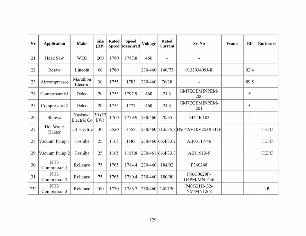
Sr Application Make Size (HP)
Rated Speed
Speed Measured Voltage Rated
Current Sr. No Frame Eff Enclosure
21 Head Saw WEQ 200 1780 1787.8 460 - -
22 Resaw Lincoln 60 1780 230/460 146/73 013203409J-R 92.4
23 Aircompressor Marathon Electric 30 1755 1783 230/460 76/38 - 89.5
24 Compressor #1 Delco 20 1755 1797.9 460 24.3 GM7EQEMINPEM-200 91
25 Compressor#2 Delco 20 1755 1777 460 24.3 GM7EQEMINPEM-201 91
26 Shinwa Yaskawa Electric Co
30 (22 kW) 1760 1779.9 230/460 70/35 344446103 - -
27 Hot Water Heater US Electric 30 3520 3558 230/460 71.6/35.8 B564AV10V253R337F TEFC
28 Vacuum Pump 1 Toshiba 25 1165 1188 230/460 66.4/33.2 AB03117-46 TEFC
29 Vacuum Pump 2 Toshiba 25 1165 1185.8 230/461 66.4/33.3 AB11913-5 TEFC
30 NH3 Compressor 1 Reliance 75 1765 1784.4 230/460 184/92 P360248
31 NH3 Compressor 2 Reliance 75 1765 1780.4 230/460 180/90 P36G0029F-
G4PM/MN1436
*32 NH3 Compressor 3 Relaince 100 1770 1786.7 230/460 240/120 P40G21H-G2-
NM/MN1268 IP
129

Sr Application Make Size (HP)
Rated Speed
Speed Measured Voltage Rated
Current Sr. No Frame Eff Enclosure
*33 NH3 Compressor 4 US Electric 40 1800 1851.9 208/416 52/104 1100101
34 High Pressure #2 Pump Leeson 20 1755 1797.7 460 24.1 n256t17fk48 - 91 TEFC
35 # 17 Injection Mold - 50 1175 1177.7 460 70 TV4688A1C - - -
36 # 17 Injection Mold - 50 1175 1188.2 460 70 TV4688A1C - - -
37 GrayMill GE 150 595 594.7 440 202 5K6335FBA2 - - -
38 Den. Gard. Recip Air Comp Baldor 25 1760 1771.2 460 32.5 M25311CW - - -
39 boltmaker duty Delco 125 855 884.6 460 187.5 4A75
40 Reliance ele 40 565 593.6 220/440 174/87 X-115677-A1 N7800Y4R
41 guard Linconln 125 1775 1778.2 230/460 146 1298248
42 Lincoln 250 1775 1769.2 460 213 3524847 -
43 #2Hyd Pump WEQ 100 1185 1189.9 460 122 AF72609 - - TEFC
*44 Air Comp WAUSAU 200 1770 1785.7 460 228 FF93504613-5 - - -
130

Sr Application Make Size (HP)
Rated Speed
Speed Measured Voltage Rated
Current Sr. No Frame Eff Enclosure
45 A Air Comp West Marathon 125 1780 1787.6 480 147 - - - -
*46 Air Comp GE 150 1785 1784 460 174 VC321029 - - -
47 #1comb. Air fan MAXSE 150 1776 1797.1 460 168 CMC13037-1 - 95 TEFC
48 furnace ejector airfan - 75 1780 1790.5 230/460 178/89 6212-2ZJC3 - 93.6 -
*49 8 Unit Press Motor 1 GE 150 1750 1781.6 460 238 SCD204SAO46A810 - -
50 Baldor 50 3525 3545 230/460 122/61 12/466000509803
51 Baldor 30 1750 1796.6 480 c0205300072
52 cold water pump US Electric 60 1780 1780.1 230/460 F216-A06A120R083M
131

APPENDIX IV SAS Codes
Code for Scatter Matrix Data Motors; infile 'D:\Documents and Settings\General\My Documents\Subodh\Thesis\Data\Motors1.dat'; input No HP RPM_R RPM_M RPM_S S Volt Curr LF_S LF_P; Title 'Data'; x1 = HP*RPM_R; x2 = HP*RPM_M; x3 = HP*RPM_S; x4 = HP*S; x5 = HP*Volt; x6 = HP*Curr; x7 = HP* LF_S; x8 = RPM_R*RPM_M; x9 = RPM_R*RPM_S; x10 = RPM_R*S; x11 = RPM_R*Volt; x12 = RPM_R*Curr; x13 = RPM_R*LF_S; x14 = RPM_M*RPM_S; x15 = RPM_M*S; x16 = RPM_M*Volt; x17 = RPM_M*Curr; x18 = RPM_M*LF_S; x19 = RPM_S*S; x20 = RPM_S*S; x21 = RPM_S*Volt; x22 = RPM_S*Curr; x23 = RPM_S*LF_S; x24 = S*Volt; x25 = S*Curr; x26 = S*LF_S; x27 = Volt*Curr; x28 = Volt*LF_S; x29 = Curr*LF_S; LF_S2 = LF_S**2; LF_S3 = LF_S**3; LF_S4 = LF_S**4; LF_S5 = LF_S**5; LF_S6 = LF_S**6; symbol1 v=dot h=.8 c=blue; proc print data = Motors; run; %include 'D:\Documents and Settings\General\My Documents\Subodh\Thesis\Data\Analysis\SAS Macros\scatmat.sas'; %scatmat(Data = Motors, Var = HP RPM_R RPM_M RPM_S S Volt Curr LF_S LF_P , Interp = RL); Run; proc print data = Motors;
132

%include 'D:\Documents and Settings\General\My Documents\Subodh\Thesis\Data\Analysis\SAS Macros\scatmat.sas'; %scatmat(Data = Motors, Var = HP S Volt Curr LF_S LF_P x4 x7 x24 , Interp = RL); Run; Quit; Code for Straight Line Model Data Motors; infile 'D:\Documents and Settings\General\My Documents\Subodh\Thesis\Data\Motors1.dat'; input No HP RPM_R RPM_M RPM_S S Volt Curr LF_S LF_P; Title 'Data'; run; proc print data = Motors; Proc REG; Title 'Straight Line Model'; Model LF_P = LF_S; Plot LF_P*LF_S; Output out=outstraight P = predicted R= residual; Run; Proc Gplot data = outstraight; Title 'Residual Plot'; symbol1 v=dot h=.8 c=blue; plot residual*predicted; plot residual*LF_S; Run; Proc Univariate data = Motors normal; probplot LF_S LF_P; Run; Quit; Code for Polynomial Model Data Motors; infile 'D:\Documents and Settings\General\My Documents\Subodh\Thesis\Data\Motors1.dat'; input No HP RPM_R RPM_M RPM_S S Volt Curr LF_S LF_P; LF_S2 = LF_S**2; LF_S3 = LF_S**3; LF_S4 = LF_S**4; LF_S5 = LF_S**5; LF_S6 = LF_S**6; run; proc print data = Motors; Proc Reg; Title 'Polynomial Regression 6th degree'; Model LF_P = LF_S LF_S2 LF_S3 LF_S4 LF_S5 LF_S6; output out = outpoly p = predicted r = residu; Run ;Proc GPLOT data =outpoly; Title 'Polynomial Regression'; plot LF_P * LF_S6; Title 'Residual Plots';
133

plot residu*predicted; Plot residu*LF_S6; Run; Proc univariate data = outpoly noprint ; Title 'QQ Plot'; qqplot residu/normal; run; Quit; Code for Multiple Regression Model Data Motors; infile 'D:\Documents and Settings\General\My Documents\Subodh\Thesis\Data\Motors1.dat'; input No HP RPM_R RPM_M RPM_S S Volt Curr LF_S LF_P; /*All 2 factor interactions*/ x1 = HP*RPM_R; x2 = HP*RPM_M; x3 = HP*RPM_S; x4 = HP*S; x5 = HP*Volt; x6 = HP*Curr; x7 = HP* LF_S; x8 = RPM_R*RPM_M; x9 = RPM_R*RPM_S; x10 = RPM_R*S; x11 = RPM_R*Volt; x12 = RPM_R*Curr; x13 = RPM_R*LF_S; x14 = RPM_M*RPM_S; x15 = RPM_M*S; x16 = RPM_M*Volt; x17 = RPM_M*Curr; x18 = RPM_M*LF_S; x19 = RPM_S*S; x20 = RPM_S*S; x21 = RPM_S*Volt; x22 = RPM_S*Curr; x23 = RPM_S*LF_S; x24 = S*Volt; x25 = S*Curr; x26 = S*LF_S; x27 = Volt*Curr; x28 = Volt*LF_S; x29 = Curr*LF_S; symbol1 v=dot h=.8 c=blue; Title 'DATA'; run; proc print data = Motors; Proc REG; Title 'Full Model'; Model LF_P = HP RPM_R RPM_M RPM_S S Volt Curr LF_S / Selection = None ; Run; Proc REG;
134

Title ' Selection Rsquare'; Model LF_P = HP RPM_R RPM_M RPM_S S Volt Curr LF_S / Selection = RSquare; Run; Proc REG; Title 'Selection Adj-Rsquare'; Model LF_P = HP RPM_R RPM_M RPM_S S Volt Curr LF_S / Selection = ADJRSQ; Run; Proc REG; Title 'Selection Cp'; Model LF_P = HP RPM_R RPM_M RPM_S S Volt Curr LF_S / Selection = CP; Run; Proc REG; Title 'Selection MaxR'; Model LF_P = HP RPM_R RPM_M RPM_S S Volt Curr LF_S / Selection = MaxR ; Run; Proc REG; Title 'Selection Forward'; Model LF_P = HP RPM_R RPM_M RPM_S S Volt Curr LF_S / Selection = Forward ; Run; Proc REG; Title 'Backward Elimination'; Model LF_P = HP RPM_R RPM_M RPM_S S Volt Curr LF_S / Selection = Backward ; Run; Proc REG; Title 'Selection Stepwise'; model LF_P = HP RPM_R RPM_M RPM_S S Volt Curr LF_S x1 x2 x3 x4 x5 x6 x7 x8 x9 x10 x11 x12 x13 x14 x15 x16 x17 x18 x19 x20 x21 x22 x23 x24 x25 x26 x27 x28 x29/Details slstay = 0.08 slentry= 0.2 selection = stepwise VIF all ; output out=outmotor p = fitted r = residual; Run; proc print; run; quit; proc gplot data = outmotor; plot residual*fitted; plot residual*x24; plot residual*LF_S; proc univariate data = outmotor noprint ; symbol1 v=dot h=1 c=blue; qqplot residual / normal; run; /* Testing for Lack of Fit of Model fitted*/ proc rsreg data = Motors; model LF_P = LF_S x24 / lackfit; run; /* Testing for Hetersoscedasticity*/ proc REG; TITLE 'Testing for Heteroscedasticity'; Model LF_P = LF_S x24/SPEC; run;
135

proc reg data = Motors; model LF_P = LF_S x24; output out = resids r = resid p = yhat; title 'Breusch Pagan Test for Multiple Regression'; proc gplot data = resids; symbol1 v=star h=.8 c=blue; plot resid*yhat; data resid2; set resids; esquare = resid**2; /* r gree ss squared residual on model variables /2 to Chi-sq */ proc reg; model esquare = LF_S x24 ; title 'Breusch-Pagan test'; run; /* Multicollinearity analysis*/ Proc REG; Title 'VIF Multicollinearity Analysis'; Model LF_P = LF_S x24/VIF ; Quit;
136

APPENDIX V This appendix gives the MATLAB graphical user interface code that was developed. function varargout = ind_motor(varargin) % IND_MOTOR Application M-file for ind_motor.fig % FIG = IND_MOTOR launch ind_motor GUI. % IND_MOTOR('callback_name', ...) invoke the named callback. % Last Modified by GUIDE v2.0 08-Sep-2004 10:48:21 if nargin == 0 % LAUNCH GUI fig = openfig(mfilename,'reuse'); % Generate a structure of handles to pass to callbacks, and store it. handles = guihandles(fig); guidata(fig, handles); % This program draws the induction motor equivalent circuit ths = 0:.0025:pi; xs1 =1.45+0.075*cos(ths); ys1 = 1.2 +0.075*sin(ths); xs2 =1.6+0.075*cos(ths); xs3 =1.75+0.075*cos(ths); xs4 =1.9+0.075*cos(ths); x5 = [0.75 0.75 .8]; y5 =[1.2 1.0 1.0]; x6 = [1.1 1.3 1.3]; y6 = [1.0 1.0 0]; xw = [0.65 0.65 1.4 1.4 0.65]; yw = [0.95 1.35 1.35 0.95 0.95]; % R_ms xr=[.5 .5 .3 .3 .35 .25 .35 .25 .35 .25 .35 .25 .3 .3 .5 .5]; yr=[1.2 1 1 .775 .75 .7 .65 .60 .55 .50 .45 .40 .375 .2 .2 0]; % X_ms thm=-pi/2:.0025:pi/2; xm=0.7+0.05*cos(thm); ym=.05*sin(thm); xxm=[xm xm xm xm] ; yxm=[.4+ym 0.5+ym 0.6+ym 0.7+ym]; x1=[0.4 .65 .7 .80 0.9 1.0 1.1 1.2 1.25 1.575 ]; y1=[1.2 1.2 1.3 1.1 1.3 1.1 1.3 1.1 1.2 1.2]; plot(x1-1.2, y1,'b', 'erasemode','none') hold on
137

axis('equal') axis off plot(xs1-1,ys1,'b', xs2-1,ys1, 'b', xs3-1,ys1,'b', xs4-1, ys1,'b') xv1=[.3 .7 .7]; yv1=[1 1 .75]; xv2=[.5 .5 .7 .7 ]; yv2=[0 .2 .2 .35]; plot(xr+.8, yr, 'b') plot(xxm+.8, yxm, 'b') plot(xv1+.8, yv1,'b', xv2+.8, yv2, 'b') x21=[3.2-.025 3.6 3.6]; y21=[1.2 1.2 .9]; x22=[-.8 3.6 3.6]; y22=[0 0 .3]; xL2=[3.55 3.55 3.65 3.65 3.55]; yL2=[.3 .9 .9 .3 .3]; plot(x21, y21, 'b',x22, y22,'b') plot(xL2, yL2,'b') x2=1.0+[0.6 .65 .7 .80 0.9 1.0 1.1 1.2 1.25 1.575 ]; y2=[1.2 1.2 1.3 1.1 1.3 1.1 1.3 1.1 1.2 1.2]; plot(x2, y2,'b') plot(1.2+xs1,ys1,'b', 1.2+xs2,ys1, 'b', 1.2+xs3,ys1,'b', 1.2+xs4, ys1,'b') xd1=[.9750 1.6]; yd1=[1.2 1.2]; plot(xd1, yd1, 'b') text(-.835,1.1625, '\circ', 'color', [0 0 1]) text(-.835,-.0375, '\circ', 'color', [0 0 1]) text(-.8, .6, 'V_{1\phi}', 'Fontsize', 8, 'color', [0 0 .675]) text(1.6, .35, 'X_{ms}', 'Fontsize', 8, 'color', [0 0 .675]) text(.9, .35, 'R_{ms}', 'Fontsize', 8, 'color', [0 0 .675]) text(-.34, .975, 'R_1', 'Fontsize', 8, 'color', [0 0 .675]) text(.6, 1.05, 'X_1', 'Fontsize', 8, 'color', [0 0 .675]) text(1.85, 1, 'R_2^\prime', 'Fontsize', 8, 'color', [0 0 .675]) text(2.9, 1.05, 'X_2\prime', 'Fontsize', 8, 'color', [0 0 .675]) text(3.7, .6, 'R_L^\prime= {R_2}^\prime(1-s)/s', 'Fontsize', 8, 'color', [0 0 .675]) %text(5.5, .6, 'V_2', 'Fontsize', 8, 'color', [0 0 .675]) %text(8.75, .6, 'S_{Load}', 'Fontsize', 8, 'color', [0 0 .675]) text(-.2, -.1, 'Equivalent Circuit per phase referred to the Stator', 'color',[0 0 .675]) hold off if nargout > 0 varargout{1} = fig; end elseif ischar(varargin{1}) % INVOKE NAMED SUBFUNCTION OR CALLBACK
138

try if (nargout) [varargout{1:nargout}] = feval(varargin{:}); % FEVAL switchyard else feval(varargin{:}); % FEVAL switchyard end catch disp(lasterr); end end %| ABOUT CALLBACKS: %| GUIDE automatically appends subfunction prototypes to this file, and %| sets objects' callback properties to call them through the FEVAL %| switchyard above. This comment describes that mechanism. %| %| Each callback subfunction declaration has the following form: %| <SUBFUNCTION_NAME>(H, EVENTDATA, HANDLES, VARARGIN) %| %| The subfunction name is composed using the object's Tag and the %| callback type separated by '_', e.g. 'slider2_Callback', %| 'figure1_CloseRequestFcn', 'axis1_ButtondownFcn'. %| %| H is the callback object's handle (obtained using GCBO). %| %| EVENTDATA is empty, but reserved for future use. %| %| HANDLES is a structure containing handles of components in GUI using %| tags as fieldnames, e.g. handles.figure1, handles.slider2. This %| structure is created at GUI startup using GUIHANDLES and stored in %| the figure's application data using GUIDATA. A copy of the structure %| is passed to each callback. You can store additional information in %| this structure at GUI startup, and you can change the structure %| during callbacks. Call guidata(h, handles) after changing your %| copy to replace the stored original so that subsequent callbacks see %| the updates. Type "help guihandles" and "help guidata" for more %| information. %| %| VARARGIN contains any extra arguments you have passed to the %| callback. Specify the extra arguments by editing the callback %| property in the inspector. By default, GUIDE sets the property to: %| <MFILENAME>('<SUBFUNCTION_NAME>', gcbo, [], guidata(gcbo)) %| Add any extra arguments after the last argument, before the final
139

%| closing parenthesis. % -------------------------------------------------------------------- function varargout = V_LText_Callback(h, eventdata, handles, varargin) % -------------------------------------------------------------------- function varargout = f_sText_Callback(h, eventdata, handles, varargin) % -------------------------------------------------------------------- function varargout = P_nText_Callback(h, eventdata, handles, varargin) %-------------------------------------------------------------------- function varargout = R_1Text_Callback(h, eventdata, handles, varargin) % -------------------------------------------------------------------- function varargout = X_1Text_Callback(h, eventdata, handles, varargin) % -------------------------------------------------------------------- function varargout = R_2Text_Callback(h, eventdata, handles, varargin) % -------------------------------------------------------------------- function varargout = X_2Text_Callback(h, eventdata, handles, varargin) % -------------------------------------------------------------------- function varargout = R_cText_Callback(h, eventdata, handles, varargin) % -------------------------------------------------------------------- function varargout = X_mText_Callback(h, eventdata, handles, varargin) % -------------------------------------------------------------------- function varargout = SlipText_Callback(h, eventdata, handles, varargin) % -------------------------------------------------------------------- function varargout = ProtText_Callback(h, eventdata, handles, varargin) % -------------------------------------------------------------------- %function varargout = N_mText_Callback(h, eventdata, handles, varargin) %--------------------------------------------------------------------- %function varargout = H_PText_Callback(h, eventdata, handles, varargin) %--------------------------------------------------------------------- function varargout = pushbuttonSolve_Callback(h, eventdata, handles, varargin) % ANALYSIS OF THE EQUIVALENT CIRCUIT % OF A THREE-PHASE INDUCTION MOTOR % % The equivalent circuit can be used to determine the operating % characteristics an induction motor. Among the important aspects % in the steady-state are the variation of current, power, losses % and torque associated with various operating conditions. Upon % entering the parameters of the equivalent circuit, performance % characteristics are obtained for the specified slip and the torque % slip curve is plotted on the screen. % %function [Rclv, Xmlv, Rchv, Xmhv, Zelv, Zehv, Ic, Io, Re, Zemag, Error] = OcScTest; Error = 0;
140

V_LHandle=findobj(gcbf, 'Tag','V_LText'); Vm=eval(get(V_LHandle,'String')); f_sHandle=findobj(gcbf, 'Tag','f_sText'); f=eval(get(f_sHandle,'String')); P_nHandle=findobj(gcbf, 'Tag','P_nText'); P=eval(get(P_nHandle,'String')); R_1Handle=findobj(gcbf, 'Tag','R_1Text'); R1=eval(get(R_1Handle,'String')); X_1Handle=findobj(gcbf, 'Tag','X_1Text'); X1=eval(get(X_1Handle,'String')); R_2Handle=findobj(gcbf, 'Tag','R_2Text'); R2=eval(get(R_2Handle,'String')); X_2Handle=findobj(gcbf, 'Tag','X_2Text'); X2=eval(get(X_2Handle,'String')); R_msHandle=findobj(gcbf, 'Tag','R_msText'); Rms=eval(get(R_msHandle,'String')); X_msHandle=findobj(gcbf, 'Tag','X_msText'); Xms=eval(get(X_msHandle,'String')); SlipHandle=findobj(gcbf, 'Tag','SlipText'); S=eval(get(SlipHandle,'String')); ProtHandle=findobj(gcbf, 'Tag', 'ProtText'); Prot=eval(get(ProtHandle,'String')); % H_PHandle=findobj(gcbf, 'Tag','H_PText'); % HP=eval(get(H_PHandle,'String')); % % N_mHandle=findobj(gcbf, 'Tag','N_mText'); % Nm=eval(get(N_mHandle,'String')); j = sqrt(-1); Z1 = R1 + j*abs(X1); Z2s= R2 +j*abs(X2); if Rms ==0 |Xms==0 Error = 1; plot(0, 0), axis off
141

text(-1, .6,'Data error: R_c an R_m cannot be zero, 0 < R_c \leq inf & 0 < X_m \leq inf', 'color', [1 0 0], 'erasemode','xor') text(-1, .25, 'Enter the correct value for R_c or X_m and try again. If neglected enter inf','color',[1 0 0], 'erasemode','xor'); return, end if S > 1 | S <= 0 Error=2; plot(0, 0), axis off text(-1, .5,'Data error: s must be in per unit in the following range', 'color', [1 0 0], 'erasemode','xor') text(-1, .25, '0 < s \leq 1. Enter the correct value for s and try again.','color',[1 0 0], 'erasemode','xor'); return, end if R2 ==0 Error = 3; plot(0, 0), axis off text(-.6, .4,'Data error: R_2 cannot be zeo, enter the correct value and try again', 'color', [1 0 0], 'erasemode','xor') return, end %%%%%%% Vmp=Vm/sqrt(3); V= Vmp+j*0; Ns=120.*f/P; Nr=(1.-S)*Ns; Ws=2.*pi*Ns/60; Wr=(1.-S)*Ws; Zrd=R2+j*abs(X2); %KW = 0.746*HP; %Sm = (Ns-Nm)/Ns; if S~= 0 RLd= R2*(1-S)/S; R2ds=R2/S; else RLd =inf; R2ds=inf; end Z2=R2ds + j*abs(X2); if Rms == inf | Rms ==0, Gc = 0; else Gc = 1/Rms; end if Xms == inf | Xms==0, Bm = 0; else Bm = 1/abs(Xms); end Y2=1/Z2 ; Ye=Gc-j*Bm; if (Gc == 0 & Bm == 0) Ze = inf+j*inf; else Ze = 1/Ye; end Yf=Y2+Ye; Zf=1/Yf; Rf = real(Zf); Xf = imag(Zf); Zin=Z1+Zf; Rin = real(Zin); Xin = imag(Zin); if (Gc ~= 0 | Bm) ~= 0 Zth= Z1*Ze/(Z1+Ze);
142

Vthc=V*Ze/(Z1 +Ze); else Zth=Z1 ; Vthc=V ; end Vth=abs(Vthc); Tth = angle(Vthc)*180/pi; Rth=real(Zth); Xth=imag(Zth); Rdd=sqrt(Rth^2 + (Xth+X2)^2); Smax=R2/Rdd; Pmax=1.5*Vth^2./(Rth+Rdd); Tmax=Pmax/Ws; I1=V/Zin; I1m=abs(I1); T1=angle(I1)*180./pi; %if real(Ze) == inf & imag(Ze) == inf I2 =I1; else if Rms==inf & Xms==inf, I2=I1; else I2= Ze*I1/(Ze+Z2); end T2=angle(I2)*180/pi; I2m=abs(I2); Io=I1-I2; Iom=abs(Io); Ao=angle(Io)*180/pi; Pcore=3*real(Ze)*Iom^2; S1=3.*V*conj(I1); SCL=3*R1*I1m^2; Pin=real(S1); Pg=3.* R2ds*I2m^2; RCL=3.*R2*I2m^2; Pm=Pg-RCL; Td=Pg/Ws; I2st = Vth/(Zth+Z2s); Pgst = 3.*R2*abs(I2st)^2; Tst = Pgst/Ws; if S ~= 1 Po=Pm-Prot; hp = Po/746; To=Po/Wr; Ef=100*Po/Pin; else, end h0 = figure('Units','normalized', ... 'PaperUnits','points', ... 'Position',[0.15 0.09 0.8 0.8], ... 'Tag','Fig2'); ax1=axes('Position',[0.2 .72 .55 .20]); % Draw the Thevenin's Equivalent circuit ths = 0:.0025:pi;
143

xs1 =1.45+0.075*cos(ths); ys1 = 1.2 +0.075*sin(ths); xs2 =1.6+0.075*cos(ths); xs3 =1.75+0.075*cos(ths); xs4 =1.9+0.075*cos(ths); x5 = [0.75 0.75 .8]; y5 =[1.2 1.0 1.0]; x6 = [1.1 1.3 1.3]; y6 = [1.0 1.0 0]; xw = [0.65 0.65 1.4 1.4 0.65]; yw = [0.95 1.35 1.35 0.95 0.95]; % R_c xr=[.5 .5 .3 .3 .35 .25 .35 .25 .35 .25 .35 .25 .3 .3 .5 .5]; yr=[1.2 1 1 .775 .75 .7 .65 .60 .55 .50 .45 .40 .375 .2 .2 0]; % X_m thm=-pi/2:.0025:pi/2; Xms=0.7+0.05*cos(thm); ym=.05*sin(thm); xxm=[Xms Xms Xms Xms] ; yxm=[.4+ym 0.5+ym 0.6+ym 0.7+ym]; x1=[0.4 .65 .7 .80 0.9 1.0 1.1 1.2 1.25 1.575 ]; y1=[1.2 1.2 1.3 1.1 1.3 1.1 1.3 1.1 1.2 1.2]; plot(x1-1.2, y1,'b', 'erasemode','none') hold on axis('equal') axis off plot(xs1-1,ys1,'b', xs2-1,ys1, 'b', xs3-1,ys1,'b', xs4-1, ys1,'b') xv1=[.3 .7 .7]; yv1=[1 1 .75]; xv2=[.5 .5 .7 .7 ]; yv2=[0 .2 .2 .35]; x21=[3.2-.025 3.6 3.6]; y21=[1.2 1.2 .9]; x22=[-.8 3.6 3.6]; y22=[0 0 .3]; xL2=[3.55 3.55 3.65 3.65 3.55]; yL2=[.3 .9 .9 .3 .3]; plot(x21, y21, 'b',x22, y22,'b') plot(xL2, yL2,'b') x2=1.0+[0.6 .65 .7 .80 0.9 1.0 1.1 1.2 1.25 1.575 ]; y2=[1.2 1.2 1.3 1.1 1.3 1.1 1.3 1.1 1.2 1.2]; plot(x2, y2,'b') plot(1.2+xs1,ys1,'b', 1.2+xs2,ys1, 'b', 1.2+xs3,ys1,'b', 1.2+xs4, ys1,'b') xd1=[.9750 1.6]; yd1=[1.2 1.2]; plot(xd1, yd1, 'b')
144

text(-.835,1.1625, '\circ', 'color', [0 0 1]) text(-.835,-.0375, '\circ', 'color', [0 0 1]) %text(1.6, .35, 'jX_{m}', 'Fontsize', 10, 'color', [0 0 .675]) %text(.9, .35, 'R_{c}', 'Fontsize', 10, 'color', [0 0 .675]) text(-.34, .975, 'R_{th}', 'Fontsize', 10, 'color', [0 0 .675]) text(.6, 1.05, 'jX_{th}', 'Fontsize', 10, 'color', [0 0 .675]) text(1.85, 1, 'R_2^\prime', 'Fontsize', 10, 'color', [0 0 .675]) text(2.9, 1.05, 'jX_2\prime', 'Fontsize', 10, 'color', [0 0 .675]) %text(5.5, .6, 'V_2', 'Fontsize', 10, 'color', [0 0 .675]) %text(8.75, .6, 'S_{Load}', 'Fontsize', 10, 'color', [0 0 .675]) text(-.2, -.15, 'Thevenin''s Equivalent Circuit per phase', 'color',[0 0 .675]) text(-.5, 1.4, ['Z_{th} = ', num2str(Rth),' + j', num2str(Xth), ' \Omega'], 'Fontsize', 10, 'color', [1 0 0]) text(1.7, 1.4, ['{Z_2}^\prime = ', num2str(R2) ' + j', num2str(abs(X2)), ' \Omega'], 'Fontsize', 10, 'color', [1 0 0]) text(3.7, .75, 'R_L^\prime= {R_2}^\prime(1-s)/s', 'Fontsize', 10, 'color', [1 0 0]) text(3.7, .45, ['{R_L}^\prime = ', num2str(RLd), ' \Omega'], 'Fontsize', 10, 'color', [1 0 0]) text(-1.2, .6, ['V_{\phi (th)} = ', num2str(Vth),'\angle', num2str(Tth) ' V'], 'Fontsize', 10, 'color', [1 0 0]) %text(2.8, 1.4, ['{I_2}^\prime = ', num2str(I2), '\angle', num2str(T2), ' A'], 'Fontsize', 10, 'color', [1 0 0]) % text(3.2, 1.4, '{I_2}^\prime \rightarrow', 'color', [1 0 0]) text(-.7, 1.7,['\bfAnalysis of the Equivalent Circuit at Slip s = ',num2str(S)], 'color', [0 0 .675]) hold off % Display the results of theequivalent circuit analysis ax2=axes('Position',[0.05 .28 .2 .34]); axis off hold on % uncomment down/// % text(0,1.125, ['V_{1(LL)} = ', num2str(Vm), ' V ', 'R_1 = ', num2str(R1), ' \Omega ', 'X_1 = ', num2str(X1), ' \Omega ',... % 'R_2 = ', num2str(R2), ' \Omega ', 'X_2 = ', num2str(X2), ' \Omega ', 'R_c = ', num2str(Rms), ' \Omega ', ... % 'X_m = ', num2str(Xms),' \Omega '], 'Fontsize', 10, 'color', [0 0 0.77]) % uncomment up ^^^^ text(0, 1.0, ['{I_2}^\prime = ', num2str(I2m), '\angle', num2str(T2), ' A'], 'Fontsize', 10,'color', [0 0 0.77 ]);
145

text(0, .9, ['I_0 = ' , num2str(Iom), '\angle', num2str(Ao), ' A'], 'Fontsize', 10,'color', [0 0 0.77 ]); text(0,.8, ['I_1 = ' , num2str(I1m), '\angle', num2str(T1), ' A'], 'Fontsize', 10,'color', [0 0 0.77 ]) text(0,.7, ['P_{in} = ', num2str(Pin), ' W'], 'Fontsize', 10,'color', [0 0 0.77 ]); text(0,.6, ['P_{cu (stator)} = ', num2str(SCL), ' W'], 'Fontsize', 10,'color', [0 0 0.77 ]); text(0,.5, ['P_{core (stator)} = ', num2str(Pcore), ' W'], 'Fontsize', 10,'color', [0 0 0.77 ]); text(0,.4, ['P_{ag} = ', num2str(Pg), ' W'], 'Fontsize', 10,'color', [0 0 0.77 ]); text(0,.3, ['P_{cu (rotor)} = ', num2str(RCL), ' W'], 'Fontsize', 10,'color', [0 0 0.77 ]) text(0,.2, ['T_d = ', num2str(Td), ' N-m'], 'Fontsize', 10,'color', [0 0 0.77 ]); if S~=1 text(0,.1, ['P_m = ', num2str(Pm), ' W'], 'Fontsize', 10,'color', [0 0 0.77 ]); text(0, 0, ['P_{rot} = ', num2str(Prot), ' W'], 'Fontsize', 10,'color', [0 0 0.77 ]); text(0, -.1, ['P_o = ', num2str(Po), ' W, ', num2str(hp), ' hp'], 'Fontsize', 10,'color', [0 0 0.77 ]); text(0,-.2, ['T_o = ', num2str(To), ' N-m'], 'Fontsize', 10,'color', [0 0 0.77 ]); text(0,-.3 ,['\eta = ', num2str(Ef), ' %'], 'Fontsize', 10,'color', [0 0 0.77 ]); %% text(0,-.4, ['T_{max} = ', num2str(Tmax), ' N-m'], 'Fontsize', 10,'color', [0 0 0.77 ]); text(0,-.5, ['s_{max} = ', num2str(Smax), ' p.u.'], 'Fontsize', 10,'color', [0 0 0.77 ]); text(0,-.6, ['T_{st} = ', num2str(Tst), ' W'], 'Fontsize', 10,'color', [0 0 0.77 ]); elseif S==1 text(0,.1, ['T_{max} = ', num2str(Tmax), ' N-m'], 'Fontsize', 10,'color', [0 0 0.77 ]); text(0,.0, ['s_{max} = ', num2str(Smax), ' p.u.'], 'Fontsize', 10,'color', [0 0 0.77 ]); text(0, -.1, ['T_{st} = ', num2str(Tst), ' W'], 'Fontsize', 10,'color', [0 0 0.77 ]); else, end % Torque Speed characteristics slip1 = Smax:-.005:.0001; if Smax > 1, Smax =1;else,end slip2 = 1:-.005:Smax; slip=[slip2, slip1]; np1 = length(slip1); np2 = length(slip2); R2d1 = R2./slip1; R2d2 = R2./slip2; Z2d1=R2d1+ j*X2*ones(1,np1); Z2d2=R2d2+ j*X2*ones(1,np2); I2d1 = Vth./(Zth*ones(1,np1)+Z2d1); I2d2 = Vth./(Zth*ones(1,np2)+Z2d2); Pgd1 = 3*R2d1.*abs(I2d1).^2; Pgd2 = 3*R2d2.*abs(I2d2).^2; Tdev1 = Pgd1/Ws; Tdev2 = Pgd2/Ws; nr1 = Ns*(ones(1,np1)-slip1); nr2 = Ns*(ones(1,np2)-slip2); if length(nr2) > 4
146

x1= 1.7*nr2(4); else x1 = 1.7*nr1(2); end y1 = 0.86*Tst; x2 = 0.96*(1- Smax)*Ns; y2 = 0.89*Tmax; x3 = 0.95*Nr; y3 =0.93*Td; fy = 0:Td/20:Td; nf=length(fy); %Td2 = KW*9550/Nm; fy2 = 0:Td/20:Td; nf2=length(fy2); fx = ones(1,nf)*Nr; fx2 = ones(1,nf2)*Nr*1.015; ax3=axes('Position',[0.365 .1 .53 .5]); plot(nr1, Tdev1, 'm', nr2, Tdev2, 'r', fx, fy,'b',fx2,fy2, 'c'),grid % plot(nr2,Tdev2,'m'),grid % plot (fx,fy,'r'),grid xlabel('Rotor speed, rpm', 'color', [0 0 0.675]) ylabel('Developed Torque, N-m' , 'color', [0 0 0.675]) title('Motor torque-speed curve', 'color', [0 0 0.675]) text(x1, y1, 'T_{st}', 'color',[0 0 0.675]) text(x2, y2, 'T_{max}', 'color', [0 0 0.675]) if Nr ~= 0 text(x3, y3, 'T_d', 'color',[0 0 0.675]) else, end if S~=1 if S >= Smax text(x1,.75*y1, ['s_{max} = ',num2str(Smax), ', s \geq s_{max}'], 'color', [1 0 0]) text(x1, .5*y1,'Motor cannot operate in this region.', 'color', [1 0 0]) else, end hold off, else, end % -------------------------------------------------------------------- function varargout = pushbuttonInfo_Callback(h, eventdata, handles, varargin) % -------------------------------------------------------------------- function varargout = pushbuttonExit_Callback(h, eventdata, handles, varargin) close all
147