load flow analysis of unbalanced radial distribution systemsethesis.nitrkl.ac.in/6391/1/e-12.pdf ·...
TRANSCRIPT
Load Flow Analysis of Unbalanced
Radial Distribution Systems
Biswajit Naik(110EE0211)
Nikhil Mudgal (110EE0210)
Somanath Behera(110EE0190)
Department of Electrical Engineering
National Institute of Technology
Rourkela
2014

National Institute of Technology, Rourkela 2 | P a g e
Load Flow Analysis of Unbalanced
Radial Distribution Systems
A Thesis submitted in partial fulfillment of the requirements for the degree of
Bachelor of Technology
In
Electrical Engineering
By
Biswajit Naik
Nikhil Mudgal
Somanath Behera
Under the Supervision of
Prof. S. Ganguly
NATIONAL INSTITUTE OF TECHNOLOGY, ROURKELA
राष्ट्रीय प्रौद्योगिकी संस्थान, राउरकेऱा PIN-769008
ODISHA, INDIA

National Institute of Technology, Rourkela 3 | P a g e
Dedicated TO
Shree Jagannath
&
My beloved Parents

National Institute of Technology, Rourkela 4 | P a g e
DEPARTMENT OF ELECTRICAL
ENGINEERING
NATIONAL INSTITUTE OF TECHNOLOGY, ROURKELA- 769 008
ODISHA, INDIA
CERTIFICATE
This is to certify that the thesis report titled “Load Flow Analysis of
Unbalanced Distributed System”, submitted to the National Institute of Technology, Rourkela by Mr. Biswajit Naik, Nikhil Mudgal,
Somanath Behera for the award of Bachelor of Technology in Electrical Engineering, is a bonafide record of research work carried out by him under my supervision and guidance. The candidate has fulfilled all the prescribed requirements. The thesis report which is based on candidate’s own work, has not submitted elsewhere for a degree/diploma. In my opinion, the draft report is of standard required for the award of
a Bachelor of Technology in Electrical Engineering.
Supervisor
Department of Electrical Engineering
National Institute of Technology
Rourkela – 769 008 (ODISHA)

National Institute of Technology, Rourkela 5 | P a g e
ACKNOWLEDGEMENT
This work was carried out at the Department of Electrical Engineering,
National Institute of Technology, Rourkela, Orissa, under the supervision of
Prof. S. Ganguly.
We would like to express our sincerest gratitude to Prof. S. Ganguly for his
guidance and support throughout my work. Without him we will never be able
to complete our work with this ease. He was very patient to hear our problems
that we were facing during the project work and finding the solutions. We are
very much thankful to him for giving his valuable time for us.
Our special thanks to all our friends who did give their time for MATLAB
Coding and providing us good company. And we would like to thank our
friends who helped us in completing our thesis in time.
We thank God for giving us the chance to pursue our academic goals and a
wonderful, complete life full of amazing people.
Finally, hearty thanks to our family member for their sacrifice that encouraged
us to proceed with the work.
Biswajit Naik
Nikhil Mudgal
Somanath Behera
National Institute of Technology, Rourkela 6 | P a g e
ABSTRACT
A thru tactic for unbalanced three-phase distribution load flow solutions
is presented in this work. The distinctive topological characteristics of
distribution networks have been fully exploited to make the direct
solution possible. For unbalanced distribution system backward sweep is
used for calculation of branch current and forward sweep is used for bus
voltage. Due to the distinctive solution techniques of the approached
method, the time-consuming Lower and Upper decomposition and
forward or backward substitution of the Jacobian matrix or Y
admittance matrix required in the traditional load flow methods are no
longer necessary. Therefore, the approached method is robust and time
efficient. Test results demonstrate the validity of the approached method.
The approach shows excessive prospective to be used in distribution
automation applications.

National Institute of Technology, Rourkela 7 | P a g e
TABLE OF CONTENTS
ACKNOWLEDGEMENT 5
ABSTRACT 6
LIST OF FIGURES 8
LIST OF TABLES 8
CHAPTER 1 9
INTRODUCTION 9
1.1 Introduction 10
CHAPTER 2 13
Unbalanced Radial Distribution System 13
2.1 Unbalanced Radial Distribution System 14
CHAPTER 3 16
Forward-backward sweep load 16
3.1 Forward-Backward Sweep Load Flow Method 17
3.2 Backward Sweep 18
3.3 Forward Sweep 19 3.4 Forward Backward Sweep Method Algorithm 20
3.5 Flow-chart of unbalanced radial distribution load flow 21
CHAPTER 4 22
RESULTS AND DISCUSSIONS 22
19 BUS SYSTEM 24
08 BUS SYSTEM 25
CONCLUSION 27
REFERENCES 28
APPENDIX 29
5.1 Datasheet of 19 bus unbalanced radial distribution system 29
5.2 Datasheet of 8 bus unbalanced radial distribution system 32

National Institute of Technology, Rourkela 8 | P a g e
LIST OF FIGURES
Title Page No
Figure2.1 Three phase line section model 14
Figure3.1. Three bus power system network 17
Figure3.2 Three phase line section 18
Figure3.3. Flow chart Algorithm 20
LIST OF TABLES
List of Tables Page No
Table 3.1: Classification of buses. 17
Table 4.1: Bus Voltage and angle in radian of 19 bus URDS. 25
Table 4.2: Total power and total line loss of 19 bus URDS in KVA. 25
Table 4.3: Bus Voltage and angle in radian of 8 bus URDS. 26
Table 4.4: Total power and total line loss of 8 bus URDS in KVA. 26

National Institute of Technology, Rourkela 9 | P a g e
CHAPTER 1
INTRODUCTION

National Institute of Technology, Rourkela 10 | P a g e
1.1 Introduction
Load flow analysis is a best as well as an elementary tool to study the power system
engineering. Network optimization, state estimation, switching, Var. planning, operational
use and planning of existing system to supply the future demand; load analysis serves the
purpose. Development of new technologies and superiority of digital world like micro-
controllers, thyristors etc. bring revolution in this field. Today we have lots of methods to
study the load flow analysis like Newton Ralphson Method, Gauss-siedel Method, Fast
decoupled method, but those methods are great match for Transmission system. But unlike
transmission system, distribution system has well-known different characteristics; some of
them are as shown below:-
Radial or weakly meshed structure;
High R/X ratios of the feeders;
Multi-phase and unbalanced operation;
Unbalanced distributed load;
Exceedingly large number of branches and nodes;
Comprehensive resistance and reactance values.
Hence there is a requirement of an efficient and robust technique to handle the deal. the
traditional load flow methods used in transmission systems; fail to meet the requirements in
both performance and robustness aspects in the distribution system applications because of
above mentioned features. Precisely, the assumptions necessary for the simplifications used
in the standard fast-decoupled Newton method [1] often losses it’s validity in distribution
systems. Thus, a novel load flow algorithm for distribution systems is desired. All of the
characteristics mentioned before must be considered, to qualify for a good distribution load
flow algorithm.
There are lots of algorithms specifically designed for distribution systems have been
suggested in the literature [2]. Most of these methods are derived from transmission
networks and based on general meshed topology. Among those methods; Gauss implicit Z-
matrix method is highly fashionable but when it comes to the distribution network, this
method does not clearly exploit the radial and weakly meshed network structure of
distribution systems and, therefore, a solution of a set of equations whose size is
National Institute of Technology, Rourkela 11 | P a g e
proportional to the number of buses is required. Several other techniques, such as the 3-ø
fast decoupled power flow algorithm [3], the Newton-Raphson method and phase
decoupled method [4] etc., have also been anticipated. Another direct approach, which
utilizes two matrices developed from the topological characteristics of the distribution
system, is proposed in this paper work.
But, the dominance of the backward and forward sweep method(BFSM); over other
solution techniques as it is fast for solving the load flow of radial distribution systems and
effective; makes it more valuable. The ill-conditioned nature arising due to high R/X ratios
of the feeders are taken care of by The “BFSM”, which eradicate the need of Fast
decoupled Newton Method and Gauss Method. This techniques model the distribution
network as a tree with the slack bus as the root. The backward sweep predominantly sums
bus current to finally evaluate the branch current. And the forward sweep is used to
calculate voltage drop, which provide updates to the voltage profile constructed from the
current estimation of the flows. Ladder Network Theory have proposed by Kersting and
Mendive and Kersting[4] to slove unbalanced radial distribution system. To solve un-
balanced radial distribution networks by Backward Forward Sweep (BFS) Method;
Thukaram et al. have proposed a three phase power flow algorithm. Ranjan et al. [5] have
used Power addition based BFS method to solve un-balanced radial distribution grids.
Recent research presented some new ideas which requires different data format or some
data manipulations to calculate the special topological appearances of distribution systems.
Another technique; known as compensation-based technique to solve distribution load flow
problems, is mentioned in [6]. Branch power flow rather than branch currents were later
used in the improved version and presented.
Deep assessment and advance techniques which focuses on modeling of the un-balanced
loads and isolated generators, was proposed in [7]. In [8], the “layer-lateral” based data
format is presented while solving the feeder lateral based model. In compensation based
technique; the new records have to be build and maintained; in addition to that, there is no
scientific association between the system control variables and system status can be found.
Thus, application of compensation-based algorithm becomes difficult.

National Institute of Technology, Rourkela 12 | P a g e
The algorithm presented in this paper is a “decent but fundamental” procedure. The only
input data of this algorithm is the line data and load data. From where we calculate the
branch current by using bus current and finally evaluate the voltage profile of different
buses. The goal of proposed thesis is developing an algorithm which can explain the
unbalanced distribution load flow directly, also consider the mutual impedance if the
system is either two phase or three phase. The time-consuming Lower-Upper
decomposition and the Jacobian-matrix or the Y-admittance matrix [9], required in the
traditional Newton Raphson and Gauss implicit Z matrix algorithms, are eradicated by this
scheme and are not necessary in the new development. The proposed system is robust and
effective and can work on any number of bus systems. The test results are shown in the end
on different-different system which establish the validity as well as feasibility of the
approached method.
National Institute of Technology, Rourkela 13 | P a g e
CHAPTER 2
UNBALANCED RADIAL DISTRIBUTION SYSTEM

National Institute of Technology, Rourkela 14 | P a g e
2.1 Unbalanced Radial Distribution System
Load flow study of Unbalanced Radial Distribution System is of a great matter of deal,
since due to unbalancing of either 3-phase or 2-phase system the effect of mutual
impedance term will arise when we compute the voltage of a bus. Unbalance system not
only leads to mutual impedance but also interact with other system also like a telephonic
system, which leads to unwanted interference between both the systems. Let’s consider an
unbalanced 3 phase distribution system model and understand the concepts and analyses it
mathematically. FIG 2.1 displays a 3-ø line section and the line parameters can be
achieved by the technique developed by Carson and Lewis. A 4 × 4 matrix, which describe
the couplings effects of self and mutual impedances of the un-balanced 3-ø line section,
can be expressed as:
[𝑍𝑎𝑏𝑐𝑛] = [
Zaa Zab 𝑍𝑎𝑐 𝑍𝑎𝑛
𝑍𝑏𝑎 𝑍𝑏𝑏 𝑍𝑏𝑐 𝑍𝑏𝑛
𝑍𝑐𝑎 𝑍𝑐𝑏 𝑍𝑐𝑐 𝑍𝑐𝑛
𝑍𝑛𝑎 𝑍𝑛𝑏 𝑍𝑛𝑐 𝑍𝑛𝑛
] (1)
FIG 2.1: Three phase line section model
After applying Kron’s reduction technique, and including the effects of the ground or
neutral wire the model can be expressed as below:-
[𝑍𝑎𝑏𝑐𝑛] = [𝑍𝑎𝑎−𝑛 Zab−n 𝑍𝑎𝑐−𝑛
𝑍𝑏𝑎−𝑛 𝑍𝑏𝑏−𝑛 𝑍𝑏𝑐−𝑛
𝑍𝑐𝑎−𝑛 𝑍𝑐𝑏−𝑛 𝑍𝑐𝑐−𝑛
] (2)
Zaa
Zbb
Zcc
Znn
Zab
Zbc
Zcn
Va
Vb
Vc
Vn
VA
VB
VC
VN
Vac
Vbn
Van

National Institute of Technology, Rourkela 15 | P a g e
The relationship between bus voltages and branch currents can be articulated as:-
[𝑉𝑎
𝑉𝑏
𝑉𝑐
] = [𝑉𝐴
𝑉𝐵
𝑉𝐶
] − [Zaa−n 𝑍𝑎𝑏−𝑛 𝑍𝑎𝑐−𝑛
𝑍𝑏𝑎−𝑛 𝑍𝑏𝑏−𝑛 𝑍𝑏𝑐−𝑛
𝑍𝑐𝑎−𝑛 𝑍𝑐𝑏−𝑛 𝑍𝑐𝑐−𝑛
] [𝐼𝐴𝑎
𝐼𝐵𝑏
𝐼𝐶𝑐
] (3)
In case any phase is absent, such as the case of two phase or single phase feeder
sections, the equivalent row and column in this matrix will contain zero values. For 2-ø
line sections with a-b, b-c and a-c phases, the relationship between 2-ø bus voltages and
branch currents can be expressed as:-
[𝑉𝑎
𝑉𝑏] = [
𝑉𝐴
𝑉𝐵] − [
Zaa−n 𝑍𝑎𝑏−𝑛
𝑍𝑏𝑎−𝑛 𝑍𝑏𝑏−𝑛] [
𝐼𝐴𝑎
𝐼𝐵𝑏] (4)
[𝑉𝑏
𝑉𝑐] = [
𝑉𝐵
𝑉𝐶] − [
𝑍𝑏𝑏−𝑛 𝑍𝑏𝑐−𝑛
𝑍𝑐𝑏−𝑛 𝑍𝑐𝑐−𝑛] [
𝐼𝐵𝑏
𝐼𝐶𝑐] (5)
[𝑉𝑎
𝑉𝑐] = [
𝑉𝐴
𝑉𝐶] − [
𝑍𝑎𝑎−𝑛 𝑍𝑎𝑐−𝑛
Zca−n 𝑍𝑐𝑐−𝑛] [
𝐼𝐴𝑎
𝐼𝐶𝑐] (6)
In case of 1-ø line sections:
𝑉𝑖𝑎 = 𝑉𝑗𝑎 + 𝑍𝑎𝑎−𝑛 × 𝐼𝑖𝑗−𝑎 (7)
𝑉𝑖𝑏 = 𝑉𝑗𝑏 + 𝑍𝑏𝑏−𝑛 × 𝐼𝑖𝑗−𝑏 (8)
𝑉𝑖𝑐 = 𝑉𝑗𝑐 + 𝑍𝑐𝑐−𝑛 × 𝐼𝑖𝑗−𝑐 (9)
The models mentioned for multi-phase distribution systems are considered in the
subsequent sections for load flow.

National Institute of Technology, Rourkela 16 | P a g e
CHAPTER 3
FORWARD-BACKWARD SWEEP LOAD
FLOW METHOD
National Institute of Technology, Rourkela 17 | P a g e
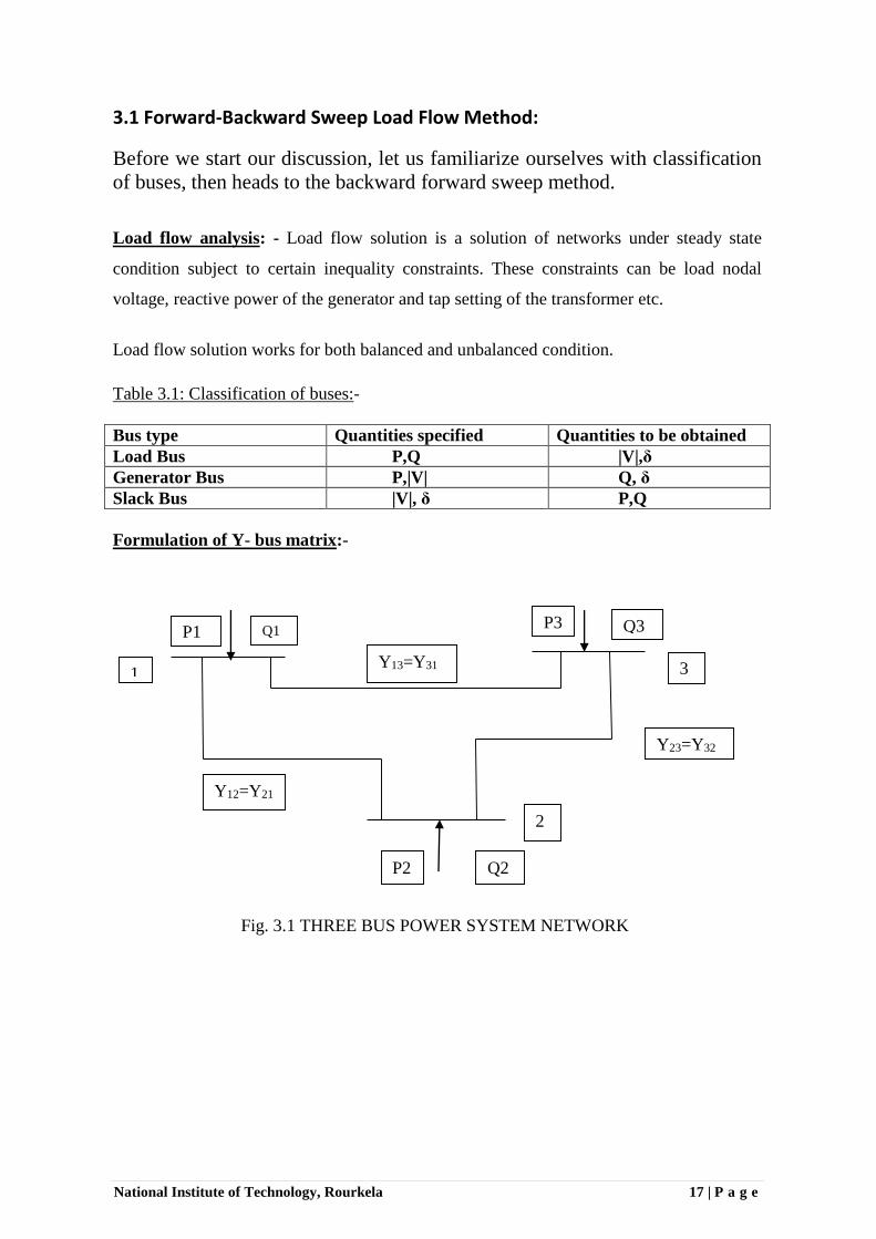
3.1 Forward-Backward Sweep Load Flow Method:
Before we start our discussion, let us familiarize ourselves with classification
of buses, then heads to the backward forward sweep method.
Load flow analysis: - Load flow solution is a solution of networks under steady state
condition subject to certain inequality constraints. These constraints can be load nodal
voltage, reactive power of the generator and tap setting of the transformer etc.
Load flow solution works for both balanced and unbalanced condition.
Table 3.1: Classification of buses:-
Bus type Quantities specified Quantities to be obtained
Load Bus P,Q |V|,δ
Generator Bus P,|V| Q, δ
Slack Bus |V|, δ P,Q
Formulation of Y- bus matrix:-
Fig. 3.1 THREE BUS POWER SYSTEM NETWORK
P2
Q3 P3 Q1 P1
Q2
1 3
2
Y13=Y31
Y12=Y21
Y23=Y32
National Institute of Technology, Rourkela 18 | P a g e
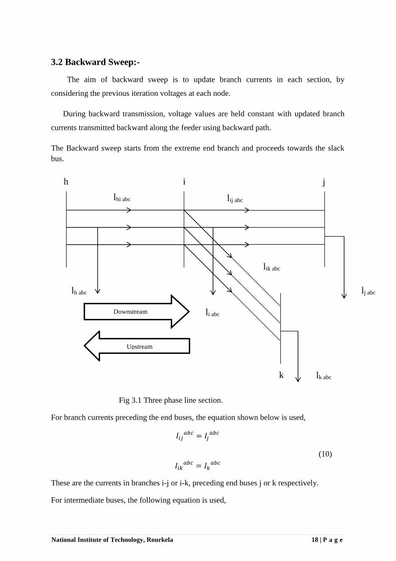
3.2 Backward Sweep:-
The aim of backward sweep is to update branch currents in each section, by
considering the previous iteration voltages at each node.
During backward transmission, voltage values are held constant with updated branch
currents transmitted backward along the feeder using backward path.
The Backward sweep starts from the extreme end branch and proceeds towards the slack
bus.
Fig 3.1 Three phase line section.
For branch currents preceding the end buses, the equation shown below is used,
𝐼𝑖𝑗𝑎𝑏𝑐 = 𝐼𝑗
𝑎𝑏𝑐
(10)
𝐼𝑖𝑘𝑎𝑏𝑐 = 𝐼𝑘
𝑎𝑏𝑐
These are the currents in branches i-j or i-k, preceding end buses j or k respectively.
For intermediate buses, the following equation is used,
Downstream
Upstream
lj abc
lk abc
li abc
lh abc
h
lhi abc
i
lij abc
j
lik abc
k

National Institute of Technology, Rourkela 19 | P a g e
𝐼ℎ𝑖𝑎𝑏𝑐 = 𝐼𝑖𝑗
𝑎𝑏𝑐 + 𝐼𝑖𝑘𝑎𝑏𝑐 + 𝐼𝑖
𝑎𝑏𝑐
(11)
𝐼ℎ𝑖𝑎𝑏𝑐 = ∑ 𝐼𝑖𝑟
𝑎𝑏𝑐
𝑟
+ 𝐼𝑖𝑎𝑏𝑐
Where,
r = all those buses connected to ‘i’ downstream.
𝐼ℎ𝑖𝑎𝑏𝑐 = Branch current vector between bus h and i.
𝐼𝑖𝑗𝑎𝑏𝑐 = Branch current vector between bus i and j.
𝐼𝑖𝑘𝑎𝑏𝑐 = Branch current vector between bus i and k.
3.3 Forward Sweep:-
The aim of the forward sweep is to calculate the voltages at each node starting from the
source node.
The source node is set as unity. and other node voltages are calculated as,
𝑣𝑏𝑖 = 𝑣𝑏𝑖−1 − 𝐼𝑏𝑖 ∗ 𝑧𝑖 − 𝐼𝑏𝑖 ∗ 𝑧𝑚𝑢𝑡𝑢𝑎𝑙𝑖 (12)
Where,
𝑣𝑏𝑖= voltage of ith bus.
𝑣𝑏𝑖−1= voltage of (i-1) th bus.
zmutual i = mutual impedance.
Mutual impedance will be present for both three phase and two phase, but it is absent for
single phase.

National Institute of Technology, Rourkela 20 | P a g e
3.4 Forward Backward Sweep Method Algorithm:-
Step 1: Read input data i.e. the line data and the load data.
Step 2: From the data, vectors bp[m], adb[m], mf[m] and mt[m] are formed. Vector bp[m]
stores the bus phases of all the buses of radial distribution grid. adb[m] with dimension
double that of number of branches, stores adjacent buses of each of the buses.
mf[m], mt[m] = acts as a pointer to adb[m]; they store the starting and ending
memory location of bus k in adb[m]; m=1,2,…….nb; nb= no. of buses.
Step 3: The magnitude of voltages is estimated as 1 p.u. for all buses, and angle 0 degree
for phase ~a,-120 degree for phase~b and 120 degree for phase~c.
Step 4: Set K=1 (iteration counter).
Step 5: Find Equivalent current injection,
𝐼𝑖𝑘 = (
𝑃𝑖+𝑗𝑄𝑖
𝑣𝑖𝑘 )
∗
; 𝑓𝑜𝑟 𝑖 = 2 𝑡𝑜 𝑖 = 𝑛𝑏. (13)
Step 6: For calculating branch current, a backward sweep from bus i= nb is carried out,
using equation (1) and (2).
Step 7: Set i= 2.
Step 8: To update magnitude and angles of bus voltage, forward sweep is applied.
Step 9: Set i=i+1.
Step 10: Check for i=nb, if yes step 11 is followed else step 8 is followed.
Step 11: Convergence is checked, for each of bus voltage magnitude by comparing with the
values of previous iteration. If convergence is achieved, then step 13 is followed
else step 12 is followed.
Step 12: K=K+1 and go to step 5.
Step 13: Print voltage magnitude in per unit and angles in radians at each bus.

National Institute of Technology, Rourkela 21 | P a g e
3.5 Flow-chart of unbalanced radial distribution load flow:
K=k+1
No
Fig 3.2:-Flow chart of URDS Load Flow.
Read input Data
From bp[i],adb[i],mf[i],mt[i]
Estimate voltage Mag.at 1P.U for
All buses and angles
00=for phase a
-1200=for phase b
1200=for phase c
k =1; I =1
Compute equivalent bus current injection
Is
mt[i]-mf[i]=0
?
Determine branch currents
preceding and buses
Find intermediate branch currents
I = 2
Forward sweep to update bus voltage (mag. And angle)
i=i+1
Is i=nb?
Has soln
converged ? Power flow and system loss
is calculated
Yes
No
No
Yes
Yes
bp[i] :Stores no. of phases
adb[i] :Stores no. of adjacent buses
mf[i] :Final bus location
mt[i] :Initial bus location
National Institute of Technology, Rourkela 22 | P a g e
CHAPTER 4
RESULTS AND DISCUSSIONS

National Institute of Technology, Rourkela 23 | P a g e
4.1 RESULTS AND DISCUSSIONS
To study the load flow analysis of unbalanced distribution system; the very nature of
balanced load’s study is essential. In unbalanced system, we consider the fact of mutual
impedance, hence the voltage drop by mutual impedance. The bus voltages and the angles
of each phase are the results obtained from MATLAB and it is shown in tabular form. In
the end, power loss of the line is calculated by square of the branch current multiply with
the real component of the corresponding impedance. The efficiency of the line after
reducing the loss, is more than 99%.
This method computes the power flow solution for its given radial network with its
loadings and illustrated with 8 bus and 19 bus system of unbalanced radial distribution
system. Also the total power and total line loss at phase a, phase b and phase c are found
out and tabulated for both 19 bus as well as 8 bus Unbalanced Radial Distribution System.
The base value considered is mentioned below:
Base KVA= 1000;
Base KV= 11;
Considering these base values the data sheet is prepared and shown in tabular form in the
Appendix section

National Institute of Technology, Rourkela 24 | P a g e
19 BUS SYSTEM:-
The line data and load data are given in Appendix. For the load flow of 19 bus system, the
base KV and base KVA are chosen as 11KV and 1000KVA respectively.
TABLE 4.1: VOLTAGE AND PHASE ANGLES OF 19 BUS URDS:-
BUS NO.
PHASE A PHASE B PHASE C
|Va|(PU) <Va(rad)
angle
|Vb|(PU) <Vb(rad)
angle
|Vc|(PU) <Vc(rad)
angle
1 1.000 0 1.000 -2.09 1.0000 2.09
2 0.9959 0.001 0.9964 -2.0943 0.9961 2.0947
3 0.9953 0 0.9963 -2.0943 0.9955 2.0949
4 0.9957 0.001 0.9964 -2.0943 0.9959 2.0948
5 0.9956 0.001 0.9963 -2.0943 0.9959 2.0948
6 0.9956 0.001 0.9963 -2.0943 0.9959 2.0948
7 0.9954 0 0.9961 -2.0942 0.9957 2.0947
8 0.9953 0.001 0.9961 -2.0942 0.9956 2.0947
9 0.9931 0.002 0.9936 -2.0940 0.9931 2.0947
10 0.9900 0.003 0.9902 -2.0938 0.9897 2.0948
11 0.9896 0.003 0.9898 -2.0937 0.9891 2.0949
12 0.9896 0.003 0.9898 -2.0937 0.9891 2.0949
13 0.9880 0.004 0.9880 -2.0936 0.9876 2.0949
14 0.9892 0.003 0.9894 -2.0937 0.9888 2.0949
15 0.9894 0.003 0.9895 -2.0936 0.9887 2.0949
16 0.9893 0.003 0.9895 -2.0936 0.9887 2.0949
17 0.9888 0.003 0.9889 -2.0937 0.9883 2.0949
18 0.9887 0.003 0.9888 -2.0936 0.9882 2.0949
19 0.9891 0.003 0.9890 -2.0936 0.9884 2.0948

National Institute of Technology, Rourkela 25 | P a g e
TABLE 4.2: TOTAL POWER AND TOTAL LINE LOSS OF 19 BUS URDS IN kW
SL. NO. PHASE TOTAL POWER IN kW TOTAL LINE LOSS IN kW
1. A 140.3866 2.0995
2. B 129.2641 2.0843
3. C 136.9657 2.1290
08 BUS SYSTEM
The line data and load data are given in Appendix.
For the load flow of 8 bus system, the base KV and base KVA are chosen as 11KV and
1000KVA respectively.
TABLE 4.3: VOLTAGE AND PHASE ANGLES OF 8 BUS URD
BUS NO.
PHASE A PHASE B PHASE C
|Va|(PU) <Va(rad)
angel
|Vb|(PU) <Vb(rad)
angle
|Vc|(PU) <Vc(rad)
angle
1 1.000 0 1.000 -2.09 1.0000 2.09
2 0.9994 -0.0002 0.9997 -2.0942 0.9987 2.0945
3 0 0 0.9991 -2.0938 0.9975 2.0943
4 0 0 0 0 0.9973 2.0943
5 0 0 0 0 0.9974 2.0943
6 0 0 0 0 0.9975 2.0943
7 0.9994 -0.0002 0 0 0 0
8 0 0 0.9997 -2.0942 0 0

National Institute of Technology, Rourkela 26 | P a g e
TABLE 4.4: TOTAL POWER AND TOTAL LINE LOSS OF 8 BUS URDS IN kW
SL. NO. PHASE TOTAL POWER IN kW TOTAL LINE LOSS IN kW
1. A 1115.9 1.0778
2. B 872.5751 1.0767
3. C 1884.3 3.9264

National Institute of Technology, Rourkela 27 | P a g e
CONCLUSION:-
In this report, a direct method for distribution load flow solution is presented to solve
load flow problem by using two matrices, BIBC and BCBV. BIBC is abbreviated form of
bus injection to branch currents, and the BCBV stands for branch currents to bus voltages.
These two matrices are collectively used to form a direct approach to solve the load flow
problems in case of balanced distribution system.
For unbalanced distribution system backward sweep is used for calculation of branch
current and forward sweep is used for bus voltage. The results of 8 bus unbalanced 3 phase
radial distribution system and 19 bus unbalanced 3 phase radial distribution system is
shown to demonstrate the algorithm.
National Institute of Technology, Rourkela 28 | P a g e
REFERENCES:-
[1] K. A. Birt, J. J. Graffy, J. D. McDonald, and A. H. El-Abiad, “Three phase load flow
program,” IEEE Trans. Power Apparat. Syst., vol. PAS-95, pp. 59–65, Jan. /Feb. 1976
[2] T.-H. Chen, M.-S.Chen, K.-J. Hwang, P. Kotas, and E. A. Chebli, “Distribution system
power flow analysis—A rigid approach,” IEEE Trans. Power Delivery, vol. 6, pp. 1146–
1152, July 1991.
[3] R. D. Zimmerman and H. D. Chiang, “Fast decoupled power flow for unbalanced radial
distribution systems,” IEEE Trans. Power Syst., vol. 10, pp. 2045–2052, Nov. 1995.
[4] W. M. Kersting and L. Willis, “Radial Distribution Test Systems, IEEE Trans. Power
Syst.,”, vol. 6, IEEE Distribution Planning Working Group Rep., Aug. 1991.
[5] C. S. Cheng and D. Shirmohammadi, “A three-phase power flow method for real-time
distribution system analysis,” IEEE Trans. Power Syst., vol. 10, pp. 671–679, May 1995.
[6] D. Shirmohammadi, H. W. Hong, A. Semlyen, and G. X. Luo, “A compensation-based
power flow method for weakly meshed distribution and transmission networks,” IEEE
Trans. Power Syst., vol. 3, pp. 753–762, May 1988.
[7] T. S. Chen, M. S. Chen, T. Inoue, and E. A. Chebli, “Three- phase co-generator and
transformer models for distribution system analysis,” IEEE Trans. Power Delivery, vol. 6,
pp. 1671–1681.2, Oct. 1991.
[8] G. X. Luo and A. Semlyen, “Efficient load flow for large weakly meshed networks,”
IEEE Trans. Power Syst., vol. 5, pp. 1309–1316, Nov. 1990.
[9] W. M. Lin and M. S. Chen, “An overall distribution automation structure,” Elect.
Power Syst. Res., vol. 10, pp. 7–19, 1986

National Institute of Technology, Rourkela 29 | P a g e
APPENDIX:
5.1 Datasheet of 19 bus unbalanced radial distribution system:
Load data:
SL.NO. BUS NO. PHASE A(PU) PHASE B(PU) PHASE C(PU)
1. 2 0.01038+0.00501i 0.00519+0.00252i 0.01038+0.00501i
2. 3 0.01101+0.00534i 0.00519+0.00252i 0.00972+0.00471i
3. 4 0.00405+0.00195i 0.00567+0.00276i 0.00648+0.00315i
4. 5 0.00648+0.00315i 0.00519+0.00252i 0.00453+0.00219i
5. 6 0.00420+0.00204i 0.00309+0.00150i 0.00291+0.00141i
6. 7 0.00972+0.00471i 0.00810+0.00393i 0.00810+0.00393i
7. 8 0.00744+0.00360i 0.00534+0.00258i 0.00339+0.00165i
8. 9 0.01230+0.00597i 0.01491+0.00723i 0.01329+0.00642i
9. 10 0.00339+0.00165i 0.00420+0.00204i 0.00258+0.00126i
10. 11 0.00744+0.00360i 0.00744+0.00360i 0.01101+0.00534i
11. 12 0.00972+0.00471i 0.00810+0.00393i 0.00810+0.00393i
12. 13 0.00438+0.00213i 0.00534+0.00258i 0.00648+0.00315i
13. 14 0.00309+0.00150i 0.00309+0.00234i 0.00405+0.00195i
14. 15 0.00438+0.00213i 0.00486+0.00234i 0.00696+0.00336i
15. 16 0.00777+0.00378i 0.01038+0.00501i 0.00777+0.00378i
16. 17 0.00648+0.00315i 0.00486+0.00234i 0.00486+0.00234i
17. 18 0.00543+0.00258i 0.00534+0.00258i 0.00552+0.00267i
18. 19 0.00876+0.00423i 0.01005+0.00486i 0.00714+0.00345i

National Institute of Technology, Rourkela 30 | P a g e
Line data (self-impedance):
SL. NO. FROM TO PHASE A(PU) PHASE B(PU) PHASE C(PU)
1. 1 2 0.0387+0.01665i 0.0387+0.01665i 0.0387+0.01665i
2. 2 3 0.0645+0.02775i 0.0645+0.02775i 0.0645+0.02775i
3. 2 4 0.01935+0.008325i 0.01935+0.008325i 0.01935+0.008325i
4. 4 5 0.01935+0.008325i 0.01935+0.008325i 0.01935+0.008325i
5. 4 6 0.0129+0.00555i 0.0129+0.00555i 0.0129+0.00555i
6. 6 7 0.0258+0.0111i 0.0258+0.0111i 0.0258+0.0111i
7. 6 8 0.03225+0.013875i 0.03225+0.013875i 0.03225+0.013875i
8. 8 9 0.0387+0.01665i 0.0387+0.01665i 0.0387+0.01665i
9. 9 10 0.0645+0.02775i 0.0645+0.02775i 0.0645+0.02775i
10. 10 11 0.01935+0.008325i 0.01935+0.008325i 0.01935+0.008325i
11. 10 12 0.01935+0.008325i 0.01935+0.008325i 0.01935+0.008325i
12. 11 13 0.0645+0.02775i 0.0645+0.02775i 0.0645+0.02775i
13. 11 14 0.0129+0.00555i 0.0129+0.00555i 0.0129+0.00555i
14. 12 15 0.0645+0.02775i 0.0645+0.02775i 0.0645+0.02775i
15. 12 16 0.0774+0.0333i 0.0774+0.0333i 0.0774+0.0333i
16. 14 17 0.04515+0.019425i 0.04515+0.019425i 0.04515+0.019425i
17. 14 18 0.0516+0.0222i 0.0516+0.0222i 0.0516+0.0222i
18. 15 19 0.0516+0.0222i 0.0516+0.0222i 0.0516+0.0222i

National Institute of Technology, Rourkela 31 | P a g e
Line data (mutual impedance):
NBR BC(× 10-3) (PU) AB(× 10-3) (PU) AC(× 10-3) (PU)
1 12.9+5.55i 12.9+5.55i 12.9+5.55i
2 21.5+9.25i 21.5+9.25i 21.5+9.25i
3 6.45+2.775i 6.45+2.775i 6.45+2.775i
4 6.45+2.775i 6.45+2.775i 6.45+2.775i
5 4.3+1.85i 4.3+1.85i 4.3+1.85i
6 8.6+3.7i 0.09189+0.9314i 5.385+4.747i
7 10.75+4.625i 0.07351+0.7451i 4.308+3.797i
8 12.9+5.55i 12.9+5.55i 12.9+5.55i
9 21.5+9.25i 21.5+9.25i 21.5+9.25i
10 6.45+2.775i 6.45+2.775i 6.45+2.775i
11 6.45+2.775i 6.45+2.775i 6.45+2.775i
12 21.5+9.25i 21.5+9.25i 21.5+9.25i
13 4.3+1.85i 4.3+1.85i 4.3+1.85i
14 21.5+9.25i 21.5+9.25i 21.5+9.25i
15 25.8+11.1i 25.8+11.1i 25.8+11.1i
16 15.05+6.475i 15.05+6.475i 15.05+6.475i
17 17.2+7.4i 17.2+7.4i 17.2+7.4i
18 17.2+7.4i 17.2+7.4i 17.2+7.4i

National Institute of Technology, Rourkela 32 | P a g e
5.2 Datasheet of 8 bus unbalanced radial distribution system:
Load data:
SL.NO. BUS NO. PHASE A(PU) PHASE B(PU) PHASE C(PU)
1. 2 0.519+0.250i 0.259+0.126i 0.515+0.250i
2. 3 0 0.259+0.126i 0.486+0.235i
3. 4 0 0 0.324+0.157i
4. 5 0 0 0.226+0.109i
5. 6 0 0 0.145+0.070i
6. 7 0.486+0.235i 0 0
7. 8 0 0.267+0.129i 0
Line data (self-impedance):
SL.NO. FROM TO PHASE A(×10-4) PHASE B(×10-4) PHASE C(×10-4)
1. 1 2 7.74+3.33i 7.74+3.33i 7.74+3.33i
2. 2 3 0 12.9+5.55i 12.9+5.55i
3. 2 5 0 0 3.87+1.665i
4. 2 7 3.87+1.665i 0 0
5. 3 4 0 0 2.58+1.11i
6. 3 8 0 5.16+2.22i 0
7. 5 6 0 0 6.45+2.775i
Line data (mutual impedance):
NBR BC(×10-4) (PU) AB(×10-4) (PU) AC(×10-4) (PU)
1 2.58+1.11i 2.58+1.11i 2.58+1.11i
2 4.3+1.85i 0 0
3 0 0 0
4 0 0 0
5 0 0 0
6 0 0 0
7 0 0 0