load testing and load rating eight state highway bridges...

J

Load Testing and Load Rating Eight State Highway Bridges in Iowa

SUBMITTED TO:

Iowa Department of Transportation

BY:

BRIDGE DIAGNOSTICS, Inc. 5398 Manhattan Circle, Suite 100

Boulder, Colorado 80303-4239 (303) 494-3230

November, 1999

Table of Contents

INTRODUCTION

INSTRUMENTATION AND TESTING PROCEDURES

DATA EVALUATION

MODELING AND ANALYSIS

LOAD RATING PROCEDURES

SUMMARY OF LOAD RATING RESULTS

·CONCLUSIONS AND RECOMMENDATIONS

BRIDGE 6723.5R029 ROBINSON DITCH - RC SLAB

Description of Structure

Instrumentation and Load Test Details

Preliminary Investigation of Test Results

Analysis and Model Calibration

Load Rating Calculations

Conclusions and Recommendations

BRIDGE 1302.6S020 WEST CEDAR CREEK - RC SLAB


lnstrume·ntation and Load Test Details





. BRIDGE 1397.5S020 LAKE CREEK - RC SLAB




1

1

2

2

3

4

5

7

7

8

9

11

13

15

17

17

18

19

23

25

26

28

28

29

30

Analysis and Model Calibration 32

Load Rating Calculations 34

. Conclusions and Recommendations 36

BRIDGE 7601.2S003 CEDAR CREEK - STEEL GIRDER 37

Description of Structure 37

Instrumentation and Load Test Details 38

Preliminary Investigation of Test Results 39



Conclusions and Recommendations 47

BRIDGE 6707.9R029 D CLEGHORN DITCH - RC SLAB 48





LoacJ Rating Calculations 55


BRIDGE 4631.1S003 EAST FORK DES MOINES RIVER- STEEL GIRDER 59







BRIDGE 9951.4S003 EAGLE CREEK- STEEL AND PS/CONCRETE BEAMS 70






Gonclusions and Recommendations 79

BRIDGE 9712.1 R020 ELLIOT CREEK - PARABOLIC RC T-BEAM 80

Description of Structure SQ





· Conclusions Recommendations 90

APPENDIX A - FIELD TESTING PROCEDURES 91

Attaching Strain 'Transducers 92

Assembly of System 93

Performing Load Test 93

APPENDIX B - MODELING AND ANALYSIS: THE INTEGRATED APPROACH 96

Introduction 96

Initial Data Evaluation 96

Finite Element Modeling and Analysis 97

Model Correlation and, Parameter Modifications 98

APPENDIX C - LOAD RATING PROCEDURES 101.

APPENDIX D - REFERENCES 104

L_

List of Figures Figure 1 Axle configuration of Iowa rating vehicles .............................................. , .... , .... .4 Figure 2 1-29 over Robinson Ditch - Instrumentation Plan ............. '. ............. , .................. 8 Figure 3 Load Configuration of Test Truck ....................... : .............................................. 9 Figure 4 Reproducibility of load test - midspan Span 2 ................................................. 10 Figure 5 Top and bottom strains at curb - East curb at midspan of Span 2 .................. 11 Figure 6 Finite element mesh - 1-29 over Robinson Ditch .................................. ~ .......... 12 Figure 7 US-20 over West Cedar Creek - Instrumentation Plan .............. : ... : ................ 18 Figure 8 Load Configuration of Test Truck .................................................................... 19 Figure 9 Symmetry of responses at bridge centerline - span 2 ....... : ... ~ ......................... 20 Figure 1 O Symmetry of slab edge responses - span 1. ·························.········ ................ 21 Figure 11 Asymmetrical responses over pier ...................... · ............ : ............................. 21 Figure 12 Inconsistent neutral axis measurement along curb ....................................... 22 Figure 13 Neutral axis of slab ........................... ~ ....................•....................................... 22 Figure 14 Finite element mesh of bridge - West Cedar Creek ...................................... 24 Figure 15 US-20 over Lake Creek - Instrumentation Plan ............. : ............................ : .. 29 Figure 16 Load Configuration of Test Truck .................................................... · .............. 30 Figure 17 Symmetry of responses at bridge centerline - span 2 ................................... 31 Figure 18 Symmetry of slab edge responses - span 1." ................................................. 31 Figure 19 Neutral axis of slab .............................. : ..................................... , ..... , ............. 32 Figure 20 Finite element mesh of bridge - Lake Creek. , .......................... : .. ; ................. 33 Figure 21 IA 3 over Cedar Creek - Instrumentation Plan .... : .......................................... 38 Figure 22 Load Configuration of Test Truck ..... : ............................................................ 39 · Figure 23 Reproducibility of load test - midspan north exterior beam.·······'·················· 40 Figure 24 Midspan response of south exterior beam .................................................... 41 Figure 25 Midspan response of interior beam ............................................................... 41 Figure 26 Non-Composite response of north interior beam at west abutment. ............. 42 · Figure 27 South interior beam near west abutment. ..................................................... 42 Figure 28 Comparison of static and dynamic test data ................................................. 43 Figure 29 Finite element mesh - IA 3 over Cedar Creek ... ·: ................ .' ....... · .............. : .. 44 Figure 30 1-29 over Cleghorn Ditch - Instrumentation Plan ........................................... 49 Figure 31 Load Configuration of Test Truck .................................................................. 50 Figure 32 Reproducibility of data during identical truck crossings ............... : ................ 51 Figure 33 Relative magnitude differences. of Span t and Span 2 strains ..................... 52 Figure 34 Flexural response of curbs ................ : ...... : .................................................... 52 Figure 35 Negative bending observed at abutment. ..................................................... 53 Figure 36 Finite element mesh of bridge - Cleghorn ditch crossing .............................. 54 . .

Figure 37 IA 3 over East Fork Des Moines River - Instrumentation Plan ...................... 61 Figure 38 Load Configuration of Test Truck ........................................................... : ...... 62 Figure 39 Reproducibility of load test - responses from two identical truck passes ...... 63 Figure 40 Midspan Exterior Beam Strain Response .... : ................................................ 64 Figure 41 Comparison of Static and Dynamic Loading .............................. : .................. 64 Figure 42 Finite Element Mesh - Des Moines River ..................................................... 65 Figure 43 IA 3 over Eagle Creek - Instrumentation Plan .................. , ............................ 71 Figure 44 Load Configuration of Test Truck ....... : ............ , .............................................. 72 Figure 45 Reproducibility of load test .. : ........................................................................ ·. 73 Figure 46 Composite Behavior of Steel Beams ............................................................. 73 Figure 47 Strain History of Steel Beam Near Abutment.. ............................................... 7 4 Figure 48 Comparison of Static and Dynamic Loading ................................................. 7 4

. :··.···

Figure 49 Finite El~ment Mesh - Eagle Creek .............................................................. 76 Figure 50 US-20 over Elliot Creek - Instrumentation Plan ............................................ 81 Figure 51 Load Configuration of Test Truck ...................................... .' ........................... 82 Figure 52 Reprodu'cibility of strain responses - midspan Span 2 .................................. 83 Figure 53 Strain histories indicating contribution.of guardrail to exterior beam.' .... '. ...... 83 · Figure 54 Symmetry of interior beam strains at midspan of span 2 .............................. 84 Figure 55 Finite element mesh of bri9ge .................................................................... : .. 85 Figure 56 Depth profile of parabolic beams ................................................................... 85 . Figure 57 Illustration of Neutral Axis and C.urvature Calculations ................................. 97 Figure 58 AASHTO rating and posting load configurations. ·················:·: .................... 103

List of Tables Table 1 List of structures ................................................................................................. 1 Table 2 Controlling load rating factors for Iowa load configurations ............................... 4

· Table 3 Comparison of BDI and Iowa DOT HS-20 Load Rating Factors ......................... 5 Table. 4 Load Test Data Files ................... '.'~·····················'··············································· 9 Table 5 Analysis and model details - Robinson Ditch crossing ..................................... 11 Table 6 Adjustable Parameter Results .......................................................................... 13 Table ?~Model Accuracy .......................................................................... ~ ..................... 13 Table 8 Ultimate strength moment capacities for slab sections and curb ..................... 14

. Table 9 Dead load and maximum live load moment on critical slab sections ................ 15 Table 1 O Load Rating Factors - Robinson Ditch ........................................................... 15 Table 11 Load Test Data Files ...................................................................................... 19 Table 12 Analysis and model details - West Cedar Creek crossing ............................. 23 Table 13 Adjustable Parameter Results ........................................................................ 24 Table 14 Model Accuracy ................................................................. : ............................ 24 Table 15 Ultimate strength moment capacities for slab sections and curb ................... 25 Table 16 Dead load and maximum live load moment on critical slab sections .............. 26 Table 17 Load Rating Factors - West Cedar Creek ...................................................... 26 I

Table 18 Load Test Data Files ... : .................................................................................. 30 Table 19 Analysis and model details - Lake Creek crossing ......................................... 32 Table 20 Adjustable Parameter Results ........................................................................ 34 Table 21 Model Accuracy ............................ ~ ........... '. ..................................................... 34 Table 22 Ultimate strength moment capacities for slab sections and curb ................... 35 Table 23 Dead load and maximum live load moment on.critical slab sections .............. 35

I (_

Table 24 Load Rating Factors - Lake Creek ..................... : .................. : ................ , ....... 36 Table 25 Load Test Data Files ...................................................................................... 39 Table 26 Analysis and model details - Cedar Creek .................................................. : .. 43 Table 27 Adjustable Parameter Results ........................................................................ 45 Table 28 Model Accuracy ...................... , ....................................................................... 45 Table 29 Ultimate moment capacities for composite model components ...................... 46 Table 30 Dead load calculations for non-composite and composite structure .............. 46 Table 31 Maximum live load moments on critical beam sections .................................. 46 Table 32 Load Rating Factors - Cedar Creek ............................................................... 47 Table 33 Load Test Data Files ................................. .' .................................................... 50 Table 34 Analysis and model details - Cleghorn Ditch crossing ....... , ......... : ................. 53

Table 35 Adjustable Parameter Results ................. ; ...................................................... 55

Table 36 Model Accuracy····'-··············:·········································································· 55 Table 37 Ultimate strength mom~nt capacities for slab sections and curb ................... 56 Table 38 Dead load and maximum live load moment on critical slab sections .............. 57 Table 39 Load Rating Factors - Clegh.orn Ditch ......................... ~ ............. ~ .................... 57 · Table 40 Load Test Data Files .................. ,.· ................ ~ ........... : ........ : ............................ 62 Table 41 Analysis and model details - Des Moines River crossing .............................. 65 Table 42 Adjustable Parameter Results ......................... : ............ '. .. , .............................. 66 Table 43-Model Accuracy ............................................................ , .................................. 66 Table 44. Ultimate strength momel')t capacities for beam sections ................................ 67 Table 45 D~ad load and maximum live load forces on critical beam sections .............. 68 Table 46 Load Rating Factors - Des Moines River ....................................................... 68 Table 47 Load Test Data Files .. · ................. : ................................................................ ;. 72 Table 48 Analysis and model details - Eagle Creek crossing ....................................... 75 Table 49 Adjustable Parameter Results .................... : .................................................... 77 Table 50 Model Accuracy .............................................................................. : ............... 77 Table 52 Ultimate strength capacities for beam sections .............................................. 78 Table 53 Dead load and maximum live load forces on critical beam sections .............. 78 Table 54 Load Rating Factors - Eagle Creek ... :" ........................................................... 79 Table 55 Load Test Data Files ................................. : .......... ; ......................................... 82 Table 56 Analysis and model details - Elliot Creek ....................................................... 84 Table 57 Adjustable Parameter Results .................................... .' .............. ; .................... 86. Table 58 Model Accuracy ............... ~ ............................................................................... 86 Table 59 Ultimate strength capacities for beam cross-sections.··············'.···················· 87 Table 60 Dead load and maximum live load moments on critical sections ................... 88 Table 61 Dead load and maximum live load shear on critical sections ......................... 89 Table 62 Load Rating Factors· due to Moment - Elliot Creek ........................................ 89 Table 63 Load Rating Factor.s due to Shear - Elliot Creek ............................................ 90 Table 64. Error Functions ............. : ........... : ................................................................... 100

•,

Introduction Bridge Diagnostics, Inc. was contracted by the Iowa Department of Transportation to perform load testing and load rating on eight highway bridges located primarily in the northern half of the state. Bridge identifications, structure type, and load test dates are provided in Table 1. These bridges were selected for load testing due to deficient load ratings with various load configurations. ·

Table 1 List of structures. Bridge Name Maintenance # Hiohway Structure Type

Robinson Ditch . 6723.5R029 1-29 RC Slab - 3 span ( 17° skew) West Cedar Cr. 1302.6S020 US-20 · RC Slab - 3 span Lake Creek\ 1397.5S020 us.:.20 RC Slab - 3 span Cedar Creek 7601.2S003 IA-3 Steel beam - 1 span Cleghorn Ditch 6707.9R029 1-29 RC Slab - ,3 span (17° skew) Des Moines River 4631.1 S003 IA-3 Steel beam - 3 span East Eagle Cr .. 9951.4S003 IA-:-3 Steel beam - .PS/C beam hybrid Elliot Creek 9712.1 R020 us.:.20 ·Parabolic RC T-beam - 3 span

·This main report provides a general discussion of the load testing, structural evaluation, and load rating procedures. Specific details for each bridge are provided in individual report sections. Additional supporting information on load testing, analyses, and load rating are also provided in the attached appendices.

Instrumentation and Testing Procedures Each bridge was instrum~nted with between 32 to 40 strain transducers. The transducer locations were selected to capture longitudinal flexure and lateral live-load transfer characteristics of each bridge. Individual instrumentation plans are shown in the following bridge sections. '·

,

. \

All sensors were applied in a completely non-destructive manner. Surface grinding was performed to remove paint on s.teel members and surface dust on concrete members. Note that concrete was not removed to expose reinforcement on the RC structures.

Strain measurements on RC members were made with extended gage lengths (12 to 24 inches) to obtain average surface strains. It is important to note theit the purpose of the strains was not to directly compute reinforcement steel stress, but simply to measure flexural responses throughout the structure and verify that subsequent analyses would . accurately represent the observed live-load di.stribution.

After each structure was instrumented, load testing was accomplished by recording strain measurements during controlled load applications. Loading was performed by slowly driving a 3-axle dump truck, with known axle weights and dimensions, over the bridge along prescribed paths. During each truck pass, the longitudinal truck position was monitored remotely and recorded with the strain data. Depending on the width of the superstructure, between two and four lateral path-locations were defined so that lateral load distribution behavior could be examined. Truck passes were performed at

1

----------------------------

least twice along each path to ensure reproducibility of the test procedures and the structure's response behavior. Additional information regarding the semi-static load

· testing procedures is provided in Appendix A

Load testing of all eight bridges was performed between the 3rd and 12th of August, 1999. In general, all instrumentation, load testing procedures and instrumentation removal was accomplished in approximately six hours for each bridge. The Iowa Department of Transportation provided all access to the underside of the structures, traffic control, and loading vehicles.

Data Evaluation All of the field data was initially examined graphically to determine its quality and to provide a qualitative assessment of each structure's live-load response. Some of the indicators of data quality included reproducibility between identical truck crossings, elastic behavior (strains returning to zero after truck crossing), and unusual shaped responses that might indicate nonlinear behavior or possible gage malfunctions. Another useful indicator of data integrity was the symmetry of responses, when applicable. For example, strain magnitudes should be similar between symmetrically placed gages and symmetrical truck paths.

In addition to a data "quality check", information obtained during the preliminary investigation was often used to determine appropriate modeling procedures for support conditions and member stiffnesses. For example, the neutral axis locations on the beams and curb elements were examined to assess how these members were interacting with the concrete decks. Composite or non-composite behavior could be immediately established from the strain measurements. In addition, the strain directions and magnitudes observed at gages near abutments were used to determine if negative moment was induced by support conditions.

It should be noted that this qualitative investigation of the data is very important for establishing the direction that the quantitative investigation should take.

Modeling and Analysis The next phase of the investigation was to develop two-dimensional finite element models for each of the eight superstructures. Once a particular model was developed, the load testing procedures that were used in the field could essentially be "reproduced" through software. A two-dimensional "footprint" of the loading vehicle was applied to each model along the same paths that the actual vehicles crossed the bridge. A direct comparison of strain values could then be made between the analytical predictions and the experimentally measured results. In general, the initial model needed to be "calibrated" until the results matched those measured in the field. The calibration process involved changing member stiffnesses, rotational restraints, and other modeling parameters and is discussed in detail in Appendix B

2

.,

Load Rating Procedures The goal of producing accurate models was to use them to predict the actual structure's behavior when subjected to the design loads. This approach is very similar to what is· typically done for producing a load rating, except that now ari accurate model is being used. All eight bridges were rated using 'the AASHTO Load Factor technique to develop both inventory and operating limits.

In some cases the rating models were changed from the final "calibrated" models by removing secondary stiffening effects that were . .considered unreliable for long-term or when heavier loads are applied. For example, rotational end-restraints provided by rocker bearings may "free up" with the passage of a very heavy vehiCle. Stiffness parameters that were removed from the calibrated are listed in the individual bridge sections. It was also likely for some structures, tf:lat the dead-load distribution was different than the observed live-load performance because of the intended or

' unintended composite behavior, beam-end restraints, and the addition of continuous RC guardrails. In these cases the models were modified to compute dead-load effects.

Load ratings were completed for the HS-20 design truck and the three Iowa design load configurations as shown in Figure 1; Load ratings were calculated for ml.iltiple-lane loading by defining several 'truck paths that induced critical load responses for the individual components. Load response envelopes containing the critical response from each truck crossing were then generated for each member. Using the principle of superposition, envelopes from truck paths separated by 12 feet were combined to obtain multiple·-lane load conditions. Responses from 3-lane loading were reduced by _ 10% per AASHTO 3.12.1. Additional details on the implemented load rating procedures are provided in Appendix C.

'•,

3

HS-20 (J2 kips) ..

AxleWgt. 8 32 32 (kips)

l 14'

* 14' l

Axle# 1 2 , 3 .

Iowa Type4 (54.5 kips)

Axle Wgt. 12.5 14 14 : '14 (kips)

~ 15' ~- 4'f4'i

Axle# 1· "2 .3 4

Iowa Type 3-3 (80 kips)

Axle Wgt .. 14.5 12 12 13.5 , 14 14 (kips)

~ 15' ~ 4' f 10' .~ 10' f 4'i

Axle# 1 2 3 4 5 6

Iowa Type 3S3 (80 kips) .

AxleWgt. .12 13 13 14 14 14 (kips)

~ 11' , * 4' *' 20' f 4't4'i

Axle# 1 2 3 4 5· 6 ,

Figure 1 Axle configuration of Iowa rating vehicles.

Summary of Load Rating Resul_ts Table 2 contains the critical (lowest) Inventory and Operating load rating factors obtained from .each bridge. All rating factors are based on multiple-lane loading.

I 2 C Tabe II" I d f f f I f I d f ontro 1ng oa ra mg actors or owa oa con 1gura ions. Structure HS-20 Type 4 Type 3-3 Type 3S3

Inv. Oper. Inv. Oper. Inv. Oper. Inv. Qper. 6723.5R029 1.65' 2.75 2.27 3.79 2.05 3.43 1.68 2.80 1302.68020 1.22 2.04 1.41 2.35 1.88 3.13 1.41 2.35 1397.58020 1.30 2.16 1.33 2.22 1.85 3.08 1.34 2.24 7601.28003 ' 2.40 4.01 2.62 4.38 3.10 . 5.17 2.83 4.72 6707.9R029 1.08 1.80 1.19 1.99 1.27 2.12 1.04 1.73 4631.18003 1.40 2.33 1.75 2.92 1.43 2.39, 1.46 2.44 9951.48003 1.62 2.71 1.87 3.12 2.00 3.33 2.08 3.48 9712.1 R020 .83 1.38 1.02 1.70 0.93 1.56 0.98 1.64

4

1.

To illustrate how the field verified load ratings compare with those obtained by standard methods (BARS program), Table 3 contains the above HS-20 Inventory and Operating rating values along with the current Iowa DOT load ratings. Iowa DOT ratings are listed for components listed as critical by BDI and BARS.

T bl 3C a e om panson o f BDI d I an owa DOT HS 20 L d R t' F t - oa a1nq ac ors. Structure HS-20(BDI) HS-20(DOT) BDI control HS-20(DOT) DOT control

Inv. Oper. Inv. Oper. point Inv. Oper. Point <BARS\

6723.5R029 1.65 2.75 0.95 1.57 Pier 0.95 1.57 3.0 1302.6S020 1.22 2.04 0.61 1.02 Span 1 0.60 1.00 2.5 1397.5S020 1.30 2.16 0.68 1.13 soan 1 0.66 1.11 2.5 7601.2S003 2.40 4.01 0.93 1.55 Span 1 int-Bm 0.93 1.55 1.5 6707.9R029 1.08 1.80 1.04 1.73 Pier 1.04 1.73 2.0 4631.1S003 1.40 2.33 0.57 1.07 Span 2 ext-Bm 0.57 1.07 2.5 9951.4S003 1.62 2.71 0.59 1.25 Ext. PS/C Bm 0.36 0.90 1.5 9712.1R020 .83 1.38 0.69 1.14 Pier Ext. BM 0.09 0.14 3.0

Conclusions and Recommendations In general, the tested bridges had favorable load ratings, indicated by the minimum Inventory rating factors being greater than 1.0. The resulting ratings appear to be representative of each structure's condition and observed performance.

The one bridge that had Inventory rating factors less than 1.0 was the parabolic RC Tbeam bridge crossing Elliot Creek in Woodbury County. The relatively low ratings are a function of the design of the bridge as opposed to the structure's performance. Shear and moment capacities of the exterior beams were calculated to be roughly one-half of the interior beam capacities. However, the exterior beams apparently carry a higher percentage of load than was intended (based on the reinforcement details). Therefore the load ratings were controlled by the exterior beam shear and moment capacities while the interior beams had very high ratings for both shear and moment. For loadrating purposes, the vehicle wheel lines were placed two-feet from the face of the.curb to generate the critical exterior beam load conditions. Whereas normal truck paths, centered in the lanes, put the wheel lines approximately five-feet from the face of the curb. This may explain why the exterior beams show no sign of distress and perform as well as the interior beams.

Seven of the eight tested structures had RC parapet/guardrails that were not part of the original structure. In each of these cases it was determined that the parapets had a significant effect on the exterior beam or slab edge stiffness and thereby altered the structures' load distribution. This was determined by the measured neutral axis locations of the exterior beams or curbs, and then verified by the calculated load distribution characteristics. On bridges having continuous parapets (without expansion joints) the effects of the parapets were included in the live-load analyses for load rating calculations. In the event that the condition of the parapets are altered, due to . environmental effects, impact, overloading, etc., it is likelythat the load distributions will be altered as well and rating factors should be modified accordingly. Therefore, the conditions of the parapets should be examined in future inspections. In no case, however, will the loss of parapet stiffness result in a structural failure.

5

Plans for the widened steel-beam I PS/C bridge (Eagle Creek - 9950.4S003) did not indicate any shear connectors. between the steel beams and the concrete deck. During the load test, however, all strain measurements indicated that the beams and deck acted fully composite. Because of the observed condition and the construction details, including the top flanges being embedded in the deck,. the deck be.ing bonded to the end-diaphragms and the beam ends being_ embedded in the end-diaphragms, the bridge was load-rated as a composite structure. It is unlikely that steel/concrete shear interface will fail, however, the condition of the bond lines should be examined during future inspections. In the event of a composite shear failure, the bond will break at the beam-ends and gradually propagate towards midspan of the beam. Given that the structure is highly redundant, a composite shear failure will not result in a structural collapse, therefore it is reasonable to assume composite action for rating purposes.

6

·.' .·· .· ... · ..

Bridge 6723.5R029 Robinson Ditch - RC Slab -~


Structure Identification 6723.5R029 Location 1-29 over Robinson DrainaQe Ditch - Monona County Structure Type RC Slab - 3 span continuous Span Length(s) 24'-5", 31 '-2", 24'-5" Skew 17° 9' L.A. (clockwise from perpendicular) Structure/Slab/Roadway 46'-0", 43'-0", 40'-0" Widths Slab Thickness Varies transversely with parabolic curve of top surface.

10 1 /2" at slab edge. 17 1 /2" at center of roadway

Curb/Parapet Detail RC curb integral with slab and RC parapet Visual condition Slab in excellent condition with minimal flexural or

temperature cracks.

7

I


Date . August 5tn 1999 Structural Reference Point X=O, Y= O at intersection of South abutment face and East

edge of slab. X direction parallel to roadway. Test vehicle direction North bound for all tests (Positive X direction) .. Start of data recording All tests start with front axle at X = -13.6'

\

Truck position Record truck position at ~very wheel revolution (10.808'). Autoclicker placed on driver side front wheel.

Lateral truck path( s) 3 truck paths were defined for the load test. The Y position refers to distance between driver side front wheel and East edge of slab.

Y1 = 13.7' Y2 = 20.6'. Y3 = 36.6'

Measurements (36) strain gages recorded at 33 Hz Gage Placement See Figwe 2. All slab ga.ges on bottom of slab. Top

parapet gages on top ~f parapet ( 42" above bottom of slab). Slab gages placed longitudinally or perpendicular to roadway.

Gage types BDI lntelliducers with extensions (18" gage length). Number of test cycles Data was recorded while the test truck crossed the bridge

at crawl speed (5 mph). Each truck path was run twice to

ABUTMEN1 BEARINGS

check reproducibility. No high-speed passes were performed due to traffic considerations.

PIER BRIDGE PIER ABUTMENT BE'ARINGS

) I - ~m -~g~ I 1),' 1?7f ~J: 17) 11 4111 I I I I I

I 4312 I I I I I Y3QJIS.6' · I I I L ! 1 I I_;

r=c=:: ..... ==::::'---Tr-1[]---,,..-:=,1 ----iz ~:. J~?J:Jr---.'f'~--~~l:1 ________ 7i 11 . 111 I . JI/ ·11

Y3_~2D~J/ !_~:_-~~~,-~~::~_/Ji ~7~ ___ ::.:t::32 ____ JJJ~----------~--j) , 11 111 , I 111 11

I . II II I

YJ.."":.13

•7:-1-/sprr-;;fiSJ 139;~:"'i.---j/~3-,,----See~-~;----~/f,J-'---------------f /

Y 1 L/2 - 111/21.... .,:J L 9· 11 I I 1

x-o Y-O

I I I I I I I +12.0 I I I I I I 3938// 11. I

1---2+·-s·-_ __.__

-------60'-0" ([, 10 ([, AlllfTMENT BEARING

"TYPICAL CURB DE1AIL

Figure 2 1-29 over Robinson Ditch - Instrumentation Plan ..

8

- .,.,··. ... :·. ~~~~~~~~~~~~~~~~~~

6.50K 9.60K 8.10K

I 11 I Tl I I I 1-i-6.9' 6.0'.

1-1 7.85K 8.95K lj_. 7.35K

I I I I I I I I

-~ 13.9' I 4.5' f--a.o I

I

Figure 3 Load Configuration of Test Truck.

Table 4 Load Test Data Files Truck STS Comments Path Data File Y1 Rob1 .dat Driver-side wheels on right shoulder line Y1 Rob2 .. dat II II II II

Y2 Rob3.dat Passenger-side wheels on right shoulder line Y2 Rob4.dat II II II II

Y3 · RobS.dat Driver-side wheels on left shoulder line Y3 Rob6.dat II II II II

Preliminary Investigation of Test Results A visual examination of the field-data was performed to assess the quality of the data and to make a qualitative assessment qf the bridge's live-load response. Conclusions made directly from the field data were:

• Responses from identical truck paths were very reproducible as shown in Figure 4. • The majority of strain measurements indicated linear-elastic live-load responses.

Gages on.top of the parapet experienced significant temperature drift relative to the magnitude of live-load strains. The drift was caused by temperature fluctuations and was magnified by aluminum transducer extensions. Normally, temperature fluctuations are not a factor during the short-term live-load tests (30 seconds). However, gages placed on top of the bridge were exposed to sunlight and the temperature change of the transducer and extensions can occur rapidly with changes in cloud cover. Gusty winds can also influence the measurements of gages exposed to solar radiation. Therefore, the top parapet gages were used for qualitative a~sessment of curb parapet cross-section properties (neutral axis) and not for model calibration.

• Live-load strains were relatively small. Maximum midspan strains were in range of 20 to 30 micro-strain. Assuming a concrete modulus of 4,000 ksi, the maximum midspan strains roughly translate into an average tensile stress of 120 psi at the bottom surface of the slab. Maximum longitudinal steel stresses computed at the gage locations (averaged over 1811

) equal approximately 600 psi.

9

',· ,·· .. ;·.····.

• Curb and longituqinal slab strains were relatively consistent with similarly-placed gages. .

• Span 2 ·slab and curb strains were typically 10 to 20 percent less than those measured at the end span strains.

• Strain magnitudes from transverse gages we're inconsistent when wheels passed close to the gages. This was a possible indication of high density of longitudinal cracks or that the strain gradient in transverse direction was too steep to be accurately captured with extended gages. Transverse strain measurements were therefore not suitable for model calibration.

• RC parapets and curb were acting integral with the superstructure, essentially providing stiffened edges along the slab. Neutral axes of the parapet were relatively consistent, with the location being 14 to 17 inches from bottom of the slab. Figure 5 · shows the consistency of relative strain magnitudes from the top and bottom curb gages: The strain drift on the top curb gage (4114) is due to temperature.change, and was verified by the response of the West curb gages. Based on this observation, curbs should be treated as beam line along edge of slab in subsequent analyses since their added stiffness affect the load paths.

(/)

I 0 ...._ u

E

z <( 0::: fl/)

~ .. - 3. l

L

0.

· :. TF' A I r·' i 1'1 FL U E N C E D I AG RAM S BRIDGE Ct:l\JTERLINE @ MIDSPAN SPAN 1 (2 PASSES @ Y2)

. '• ······················-···········--·················-·-···························

20. 40. 60. 80. 100.

TRUCK .POSITION (ft.) 3876: 1 ............. ;?.~.7..?..:.12 ............ .

Figure 4 Reproducibility of load test - midspan Span 2.

10 .

. : ._ .. ,.

120.

,-... c 0 ,_

Ul

I 0 ,_ u

E

z <( O'.: fen

STRAIN INFLUENCE DIAGRAMS EAST CURB @ MIDSPAN OF SPAN 2 - TRUCK PATH Y1

20 . .---~~~~~~~~~~~~~, ~~~~-.~~~~-,~~~---,

..-··"··-._.;,....-- BOTTOM !SLAB GAGE (38?3) . 1 . . 10. ······························-;·-······························'···············: ................. ;.:.-•. :.-·························>················ ············································!

:····

o. 20. 40. 60. 80. 100. 120.

TRUCK POSITION (ft.) 4114: 1 ............. ;?.~.?.:?.: .. ~---··········

Figure 5 Top and bottom strains at curb - East curb at midspan of Span 2.


Table 5 provides details regarding the structure model and analysis procedures. A discussion of the analysis results is provided along with conclusions regarding the structural performance.

Table 5 Anal sis and model details.- Robinson Ditch cross in Linear-elastic finite element - stiffness method.

Model components • RC slab represented by quadrilateral (skewed) plate elements. Plate thicknesses vary in 1" increments to account for roadway crown. 1" of concrete overlay added to original RC slab thickness.

• Curbs simulated by beam elements. Cross-section included . parapet, curb, and portion of slab necessary to obtain reasonable neutral axis location (15" from bottom of slab). The beams were assumed to lie in the plane of the deck so the moment-of-inertia properties were computed about the centerline of the slab.

• Abutment and pier caps represented by rectangular beam elements.

• Elastic spring elements with eccentricity terms used to simulate rotational restraint of pile foundations. Due to construction details, spring used to provide resistance in horizontal translation. The horizontal resistance combined

. 11

with the eccentricity term provides moment resistance. Live-load 2-D footprint of test truck consisting ~f 10 vertical point loads.

Truck paths simulated.by series of load cases with truck moving at 5-foot increments.

Dead-load · Self-weight of slab, curbs, and parapets with additional 15 psf to account for overlay not included in slab thickness. (Used for load ratino only)

Data comparison 22 longitudinal strain gage locations defined on model (bottom of slab and curb): Strains computed for 16 truck positions along each path. 22x16x3 = 1056 strain values. Strain records extracted from load test data files .corresponding to analysis truck positions.

Model statistics 1000 Nodes 1302 Elements 18 Cross-section/Material types 48 Load Cases -

22 Gage locations Adjustable 1 Young's modulus (Ee - ksi) parameters for 2 Curb stiffness (lb - in4

)

model calibration ' 3 Abutment pile resistance to horizontal translation (Kx - kips/in) 4 Pier pile·resistance to horizontal translation (Kx - kips/in)

3878 405f, 43 il 4123

Figure 6 Finite.element mesh - 1-29 over Robinson Ditch.

A model with the ·above parameters was defined and the analysis program simulated the load testing process. The accuracy of the model was defined by comparing the 1056 computed and measured strain values. Selected parameters were modified to minimize the comparison error.

12

------------------------------ -

The translation spring stiffnesses used to simulate the abutment .and pier were aligned parallel to the roadway. The springs were given an eccentricity value equal to the distance between the bottom of the slab and the assumed elastic neutral axis location. The eccentricity term provided a moment-arm such.that any translational resistance would induce moment restraint. This.method of modeling the support conditions was chosen over rotational springs because it was _most representative of the actual construction. Reinforcement dowels, tying the slab to the support elements, were not

· · shown in the plans, therefore a pure moment restraint could not be justified ..

Table 6 contains the original stiffness ·parameters· and the final values after the model 9alibration process. Statistical accuracy values associated with the initial and final models are provided in Table 7. The resulting accuracy terms were in the typical range for RC slab structures.

T bl 6 Ad. t bl P a e IJUS a e t R It arame er esu s Stiffness Parameter Units Initial Value Final Value

Slab modulus E ksi 3200 4000 Curb (I) ln4 117400 105000 Abutment (Kx) Kips/in 0 550 Pier (Kx) Kips/in 0 3000

T bl 7 M d I A a e o e ccuract Statistical Term Initial Value Final Value

Absolute Error. 1677µ8 943ue · Percent Error 40.5% 13.0% Scale Error 6.5% . 4.1%' Correlation Coefficient 0.93 0.95


Load rating factors were computed for the slab components of the superstructure using the Load Factor method. A Load Factor of 1.3 was applied to all dead-load affects for both Inventory and Operating load ratings, while load factors 2.17 and 1.3 were applied to live-load responses. Ultimate strength member capacities, based on AASHTO specifications for reinforced concrete beams and slabs; were computed for positive and negative moment regions. Positive moment capacities were obtained for midspan cross-sections and negative moment capacities were computed for slab cross-sections at the face of the pier caps.

Estimated capacity calculations were made for the curb/parapet in positive and negative moment since 'it was determined that they had significant effect on the load transfer. However, due to lack of structural information on the concrete parapets, the computed capacities are assumed to be overly conservative. ltwas assumed that the parapet or railing did not contribute to the negative moment capacity of the curb - only the top curb steel was used in ultimate moment computations.

Table 8 contains slab moment capacity calculations for various different slab thicknesses. Grade 40 reinforcement, with a minimum yield stress of 40 ksi, was

13

assumed based on the age of the structure. A concrete strength of 4 ksi was allowed due the relatively high concrete modulus obtained from the model calibration process. All slab moment capacities are computed for unit width sections (1 in.).

T bl 8 Ult" t t a e 1ma es reng th t T f I b momen capac1 1es or s a f sec ions an d b cur . Section Ultimate Moment Capadties per unit slab width ·

t + Cover (in) d (in) p + M (k-in/in) d' (in) p' - M (k-in/in) 12 + 1 10.875 .0137 52.2 9.81 .0125 -39.0 13 + 1 11.875 .0126 57.6 10.81 .0113 -43.4 14 + 1 12.875 .0116 63.0 11.81 .0104 -47.8 15 + 1' 13.875 . 0108 68.3 . 12.81 :0095 -52.2 16 + 1 14.875 .0100 73.7 13.81 .0089 -56.6 17 + 1 ,' 15.875 . . 0094 79.1 14.81 .0083 -61.0 17.5 + 1 16.375 .0091 81.8 15.81 .0080 -63.2 Curb/Parapet 40.0 .025. 11681.0 21.25. .0050 -~100.0

Load rating calculations were performed for the HS-20 and the three Iowa rating vehicles by applying the truck configurations to the calibrated model. Due to the width of the roadway, three truck paths were defil'.led. The first path was defined by placing a wheel line 2 feet from the face of the curb. Subsequent truck paths were defined at 12-foot increments. Single lane loading envelopes (critical responses)' were generated for every model component by moving the applied rating truck a_t 2-foot intervals along the length of the bridge. Multiple Jane load conditions were obtained by the principle of superposition. The response envelopes were added to generate two and three-lane loading response envelopes. Three-lane load responses were reduced by 10% according to AASHTO specification 3.12.1.

Dead load responses were obtained by computing the self-weight of the structure and adding 15 PSF to account for concrete overlay not included in the slab model components. The model was adjusted prior to dead load application in that spring stiffnesses, providing rotational restraint at support locations, and edge stiffnesses, simulating the curb and parapet effects, were eliminated. Table 9 contains computed dead load and the-various rating veh.icle live-load forces for each critical slab component. Inventory and operating rating factors for each component are listed in Table 10.

14

. :· ... · '.-· ..... · ....

/\

Table 9 Dead load and maximum live load moment on critical slab sections. Slab Section Dead-Load HS-20· · Type4 Type 3-3 Type 3S3

M (k-in/in) M (k-inlin) · . M (k-in/in) M (k-in/in) M (k-in/in) 12" midspan 8.92 2.72 2.19 1.77 2.02 13" midspan 9.00 4.61 3.73 2.98 3.44 14" midspan 9.21 6.53 5.22 '4.26 5.39 15" midspan 11.73 7.71 . 6.79 5.17 6.54 16" midspan 9.96 9.59 8.14 6.08 7:90. 17" midspan 10.69 11.22 9.59 7.19 9.55 17.5" midspan 11.12 11.18 10.44 7.85· 9.69 12" pier face -22.29 -1.21 -0.83 -1.00 -1.27 13" pier face -13.04 -3.59 -3.18 -3.17 -3.47 14" pier face :..12.17 -5.33 -3.91 -3.90 -4;26 15" pier face "-14.77 -6.47 -5.06 -5.40 -6.10 16" pier face -14.21 -7.75 -5.89 -6.28 -7.51. 17" pier face -14.41 -9.09 -6.63 -7.29 -8.93 17.5" pier face -14.03 -9.43 -6.96 . -7.60 -9.33

T bl 10 L d R f F t a e oa a inQ ac ors - Rb' 0 ins on IC.

Slab Section HS-20 ·Type 4 Type 3-3 Type 383 Inv. Oper. Inv .. Oper. Inv. Oper. Inv. Oper.

12" midspan .5.18 ·8.65 6.57 10.97 8.34 13.92 7.32 12.22 13" midspan 3.37 5.63 4.42 7.38. 5.53 9.22 4.78 7,99 14" midspan 2.75 4.59 3.45 5.76 4.44 7.42 3.51 . 5.86 15" midspan 2.39 3.99 2.93 4.90. 3.88 6.48 3.07 5.12 16" midspan 2.38 3.97 2.58 4.30 3.44 5.73 2.78 A.63 17" midspan 2.11 3.51 2.38 3.97 3.15 5.26. 2.47 4.12 17.5" midspan 2.09 3.49 2.27 3.79 3.02 5.04 2.45 4.08 12" pier face 2.94 4.91 4.26 7.11 ' 3.55 5.93 2.81 4.68 13" pier face 2.61 4.36 . 3.13 '.5.22 2.96 4.94 2.70 4.51 14" pier face. 2: 13 3.55 2.62 . 4.38 2.45 4.09 2.24 3.74 15" pier .face 1:81 . 3.02 2.43 4.05 2.17 3.62 1.92 3.20 16" pier face 1.74 2.91 2.36 3.94 2.15 3.59 1.80 3.00 17" pier face 1.65 2.75 . 2.29 3.82 2.05 3.43 1.68 2.80 17.5" pier face 1.69 2.82 2.27 3.80 2.10 3.50 1.71 2.85 Curb@ pier- 1.14 1.90 1.65 2.75 '1.37 2.30 1.09 1.81 Critical RF 1.65 2.75 2.27 3.79 2.05 3.43 1.68. 2.80 - Rating of curb/parapet over pier not allowed to govern structure load rating.


The load test and structural assessment results illustrate how components not intended to be structural members often affect the structure's load distribution. The lowest rating factors were obtained for the curb elements in negative moment over the piers. However, due to the over-conservative moment capacity calculation (parapets and railing not contributing), it is not recommended that the curb rating factors be used to

15

I'. j ~··

control the superstructure rating. Of the slab components, all rating factors were controlled by the negative moment capacity at the face of the. piers.

Due to the high degree of redundancy associated with slab structures, failure of the curb elements will not result in a failure of the entire structure. It is recommended, however, that the condition of the curbs be thoroughly examined during future inspections. Excessive cracking. of the parapets and curbs over the piers would be an indication that the bridge has been heavily loaded and that the response behavior of the bridge has changed.

The load rating factors presented in this section are based on the structure's condition aMhe time of load testing. Any structural degradation must be considered in future load ratings: Note that no effort was made to assess the condition or capacity of the substructure elements such as the abutments or ·piers.

16

Bridge 1302.65020 West Cedar Creek - RC Slab


Structure Identification 1302.6$020 Location US 20 over West Cedar Cr. (drainage ditch 83) ,

Calhoun County, Iowa Structure Type RC Slab, 3-span continuous Span Lenath(s) 21 '-4" J 27'-4" J 21 '-4" Skew Perpendicular Structure/Slab/Roadway 36'-0", 34'-0", 30'-0" Widths Slab Thickness Varies transversely - parabolic curve at top surface.

11" at edge of slab. 14 1/2" at centerline of bridae.

Curb/Parapet Detail RC Curb attached with shear keys and stirrups. RC Parapet with expansion joints. Aluminum railing .

Visual condition Overall appearance is good. Minimal cracking on bottom of slab, no apparent spallina, no exposed reinforcement.

17

_J


Date August 5th, 1999 I

Structural Reference South-west corner of slab at inside face of abutment. Point Test vehicle direction East for all truck passes. Start of data recording X = -14.64 ft. Face of abutment, back 10', back 1/2 wheel - --~ revolution.

Truck position Record truck position at every wheel revolution (10.808'). Autoclicker placed on driver side front wheel.

Lateral truck path(s) .2 truck paths were defined for the load test. The Y position refers to distance between dfiver side front wheel and south at edge of slab. The two load paths were approximately symmetric about the bridge centerline.

Y1 = 5.6 ft Y2 = 28.3 ft (5.7' from no'rth edge of slab)

Measurements (40) strain gages recorded at 33 Hz -Gage Placement See Figure 7. 28 locations on bottom of slab, 8 locations on

top of curb or parapet, 4 locations on top of slab. Slab gages placed longitudinally or perpendicular to roadway.

Gage types BDl'lntelliducers with extensions (12" gage length). · Number of test cycles Data was recorded while the test truck crossed the bridge at

crawl speed (5 mph). Each truck path was run twice to check reproducibility. No high-speed passes were performed du.e to traffic considerations.

x 'll'-

SP~ l

Figure 7 US-20 over West Cedar Creek - Instrumentation Plan.

18

7.6K 8.BBK 8.BBK

I I I l 1· 11 I

6.8' 6.0' I 8:88K 8.88K

1_l I 7.6

_LI I 11 I I I I

I _j ~ 1- 14.4' . 4.5' I


Table 11 Load Test Data Files Truck STS Comments Path Data File Y1 WCED1 .DAT Test truck crossin Y1 WCED2.DAT Test truck crossin Y2 WCED3.DAT Test truck crossin Y2 · WCED4.DAT Test truck crossin

Preliminary Investigation of Test Results·

A visual examination of the field data was performed to assess the quality of the data and to make a qualitative assessment of .the bridge's live-load response. Conclusions made directly from the field data were: · • Symmetry ofstructure, truck paths, and instrumentation allowed for a direct data

comparison of similar gages. Midspan gages located along the structure's centerline measured highly symmetrical responses (Figure 9). The other gages located across the slab provided reasonably consistent strain magnitudes, but not as symmetric as the centerline gages (Figure 10). This is to be expected since the strains are dependent on the local slab properties, which can vary significantly from point to point. Large variations in symmetry were obtained at a few locations.

• Centerline gages near the pier provided less symmetry than the midspan gages, this is an indication that the slab stiffness varies significantly in the negative. moment region (Figure 11 ). Excessive cracking could possibly cause this, or variations may be due to· slab repairs. The relatively low strain magnitudes do not indicate a high degree of flexure.

• Neutral axis measurements along the curb varied significantly from location to location. Curb responses near the pier indicated nonlinear behavior, as evidenced by an inconsistent ratio of top and bottom curb strains and peak strains being slightly out of phase to each other (Figure 12). It is evident that the parapet contributes to the curb stiffness, however, parapet contribution should not be allowed during load rating analysis due to the presence of expansion joints and a nonlinear response.

19

• Strains measured on top of the slab Were used to estimate its neutral axis location (Figure 13). All top gages that were exposed to the sun had some drift during the tests and were used for qualitative purposes only.

• Span 2 strain magnitudes were approximately 75% greater than Span 1 strains. • Strains near abutment indicated minimal end-restraint provided by slab bearing.

Strains were typically caused by positive flexure throughout load cycle and in some cases dissipated entirely when truck was on the middle span.

(fl

I 0 .... u

z <( 0::: r(/1

STRAIN INFLUENCE DIAGRAMS SPAN 2 CENTERLINE GAGE - TRUCK PATHS 1 AND 2

:~. ~ __ -___ -____ -_-_-__ -___ -_-___ -__ -__ -___ ~~-_-____ -____ - __ -___ -___ -____ -___ -___ - __ -_~·/--:: __ --~--- __ ~.;-____ -____ -___ -.. ~-.:-~,-c:------:-~~;.-___ -____ -_-____ -____ -___ -___ -___ -____ -----,·····I

I 30. <--------------· · ........................................................ ········· j

------ -- -·- - . . - .. , .. --·---------·----·-·-- -------·-·-------·---··-------------·---·--···----·------·----··-· ----1

~ ·: . I . . :·. ;

----------·--·- -------------------:/---- -------·---------------------------·------ __ _:__ -----------------------------------~--------------------------------------/

I

o.

-10 I 0. 20. 40. 60. 80_ 100.

TF;ucK POSITION (ft.) 40":-7: i -------------~_Q_?._?__:_;? ____________ _

Figure 9 Symmetry of responses at bridge centerline - span 2.

20

(fl

I 0 ...... u

E

:z: <( 0::: f(/)

STRAIN INFLUENCE DIAGRAMS NORTH & SOUTH CURBS @ SPAN 1 - TRUCK PATHS 1 & 2

18. ·································:········~-·:'.>,. ·--~~~~-~--~~-~-~t ... ~~~-~-~--~--~-~---···.[ .............. ·······················

: :. ••••••• m····················••I,t\;••••••••••••l••~····SOUTH C~RT TR~~"®: Y1 I••··································

:• L•••.z···············j ······················ ·.·············::···~;;;::·~=;~~··;~=;:··~··~;································ ~ . . ............. -\:···-~;,_··:::;···· ......................... L. .................................... f ······································

~ SOUTH:CURB - TRUCK@ Y2 ' .• --·~"'"'""""'";;,.~;,;;.~ ···············•······································< ··················

0 . . .. ~.~ ··.-·.···:. ···~··:... '

-3. r .................. ········ ~

···································!

I -6.

0. 20. 40. 60. 80. 100.

TRUCK POSITION (ft.) 2139: 1 ............. ~_1 .. :3.si.:.? ........... . . ............ ~.Q.?..El:.} ............ . .. - ·-· _ :i_q?.s_:_z ____ . -

Figure 10 Symmetry of slab edge responses - span 1 .

·-0 '--

(fl

I 0 '-u

E

:z: <( 0::: t-(/)

10

STRAIN INFLUENCE DIAGRAMS CENTERLINE GAGE NEAR PIER - TRUCK PATHS 1 & 2

TRUCK @ Y2

0. ..

K/···/\. l\ I _, 0 . ~ .... \.~/---·····\· . .. ....... / ·· --~~-- ............................... , ... ..:.. ............................... L ............... .............. -j

·...... I \ ./

_,,. ···································· ·················;······· .. · ..•.. ············· .... /L. ····························+ .............................. .

- 30 . TRUCK·-~--~1·---~~~-_,,..- .............................. ,. ............. ·: .. L ........ r .......................................... .

-40

0. 20. 40. 60. 80. 100.

TRUCK POSITION (ft.) 3935:1 ............. :?.9..:3.5-:.~ ............ .

Figure 11 Asymmetrical responses over pier.

21

Cf)

I 0 ~

u

z <( O::'. t(f)

STRAIN INFLUENCE DIAGRAMS TOP & BOTTOM OF CURB NEAR PIER - TRUCK @ Yl

12 . .--~~~~--..,--~~~~~~~~~~~~~~~~~~~~~~~~~~~

____J-- TOP OF R~ CURB

9 ...... ····················· . : . :

. : : .. I 6. . .... ······················· ··~································1···· ·············· ···········; ······························ ~--·····························t·······························

~ j : j . 3 . .. . . .. ... . ... . ... /............ .. . . . . : ......... ··············· .... ; ... ~ .. ... . ...... >::'"'·"-~'·'.•;.;,;;.~;~;~,:,:;.: ..................... .

....... .. .... ~ ......................... ~··::. .... ~ .. 0. f--__..~-~-~~~-=.-~--,~~<-~~~~-!~!~~~,~~~~---'~~~~~-+-~.f-.:.~-="""'"~~~~.....:..:..~

~ / ./·.; ....... ~ . . . . . . . . --·· ·+. -. -_·_ -~":!-.. ,~-;s.~;~;:•·':( -....... ~- ~.- ......... -..... ·l·. ---- .. \. -~- .......... -········· ..... ·-· ... ; . ---i~ ... ------ .... -- ........ --~ ............ -....... . -3.

- 6 ~-·················· .......... ~ .. ; ... :, ..........• /············\·:····························:/·-···························~---····························l ~ ~~ i

-9. i--··················· ························· ········· ···························~"'.:··························'··'·······························+·················· ············! ~ . : : !

2 ~ . . .......................... : ... ;; .................... / ..... : ..........................•.... .:.. .............................. j

~::• r m ;m mm mm' \;.:/=+= ~~~~~~;;;~~~mmmm' -20. 0. 20. 40. 60. 80. 100.

TRUCK POSITION (ft.) 4113:1 ............. :3.~.'.'..f?..•.~---··········

Figure 12 Inconsistent neutral axis measurement along curb.

Cf)

I 0 ~

u

:z <( O::'. ~ c.n

STRAIN !NFLUENCE DIAGRAMS TOP AN[I BOTTOM OF SLAB - SPAN

60. ~

50. f·· ....... . ~.

40. ~-· f-

30. ··················· .. ····················~······································'.···························

..

20. ....... ·:·.... . ~~ .......... l..;::· ...... .. . . ~: .......... ·:· ·························---~---·······················-·····--···· ; ......................... . .~·

1 0 ! ·········· ............. :::::-:·~; ..... . . ~······· ~-~·-···-···_··········:······································'··························

~

' ~ / - 1 o. I· · ·· ········ -·~::/ ····'· · ., .... \ ······ ····· . ./

........... '~' ···········j································-·-····i······································

""' ..................... ~ ........................ -............. ~ .................................... . -20.

TOP OF SLAB

-30. o. 20. 40. 60. 80. 1 00.

TRUC~ POSITION (ft.) 3876: 1 ............. :3.~-~-CJ.•.-~ ............ .

Figure 13 Neutral axis of slab.

22


Table 12 provides details regarding the structure model and analysis procedures. A discussion of the analysis results is provided along with conclusions regarding the structural performanc~.

T bl 12 A I . a e na1ys1s an d d I d ·1 W C d C k mo e · eta1 s - est e ar ree crossing. Analysis type Linear-elastic finite element - stiffness method. Model geometry Plane grid matching slab plan (see Figure 14) Model components· .. RC slab represented by quadrilateral plate elements. Plate

thickn.esses vary in 1" increments to account for roadway crown. 1" of.concrete overlay added to original RC slab thickness.

• Curbs simulated.by beam elements. Cross-section included parapet, curb,· and portion of slab necessary to obtain reasonable neutral axis location (15" from pottom of slab).

• Abutment and pier caps represented by rectangular beam elements. ''

• Elastic spring elements used to simulate pile foundation . Abutment springs resist horizontal translation, whereas pier springs resist rotation and translation.

Live;..load 2-D footprint of test truck consisting of 10 vertical point loads.

I

Truck paths simulated by series of load cases with truck moving at 5-foot increments.

Dead-load Self-weight of slab, curbs, and parapets with additional 15 psf to. account for overlay not included in slab thickness. (Used for load rating only)

Data comparison 22 longitudinal strain gage locations defined on model (bottom of slab and curb). Strains computed for 23 truck positions along each path. 22x23x2 = 1012 strain values. Strain records extracted from load test data files corresponding to analysis truck positions.

Model statistics 864 Nodes 1077 Elements 19 Cross-section/Material types 46 Load Cases 22 Gage locations

Adjustable 1 Slab stiffness (Ee - ksi) Span 1 parameters for 2 Slab stiffness (Ee) over pier

'I

model calibration 3 Slab stiffness (Ee) Span 2 4 Effective Curb stiffness with parapet (I - in4

) ·

5 Effective cub stiffness at parapet expansion joints (I - in4)

6 Abutment pile longitudinal resistance (Kx -·kips/in) 7 Pier pile rotational resistance (Kr - kip-in/rad)

An initial model with the above parameters was defined and the analysis program simulated the field load test process. The accuracy of the model was defined by

23

comparing the 1012 computed and measured strain values. Selected parameters were · modified to minimize the comparison error.

Table 13 contains the original stiffness parameters and the final values after the model calibration process. Statistical accuracy Veilues associated with the initial and final models are provided in Table 14. The resulting accuracy terms were in the typical range for RC slab structures.

4058 4114 4050 . ' ' . ' . . . . . ' ' ' ' : :

3 fffl FJTilJ:] !·~---+------+ fF[l::: ---l i i 3.32. i ; ;Al-1 : ~ __._.~____.._~._..__.._._.___. !~ ~ ! ~ ! : H: ; : : . H: : : : : H :

:~:::t:::~::::t ___ :::::::::::::::::.:::_:: ::::,::: 1.~~-------------i ::::o:::: i ::::pj::::f1::::: . ! 'Wt---o----+---+-,-•,,___.__,_._.__..,~, _._,-.~. ~,~,~4

J~:rttr::~:::::::::~r::~::: ::~ ~: 1 ::::j::~:~:i l r:::~::::i --+-t---·---·--+·---·---·---·---· ~---~--- -~~ :----~.' ,----n----· : '----H----;

--------- -·---- ·----------+------·-' ' . ' . . . . . . . ' . . ' . ' . ' ' . ' . .

•~,~:.:::=:::·.,3.-~1.,·:_8_:_::.___i .. ,:~: ... :.:::1:. 1 .. -~1 .... :_1_:_:.:. J.::: ~_i_ .•.• '.8_:_~1 ~.:.: -----;l::::~HM· .. ·. , ::::, .... :. 38 :~:.,.,·. + :1+rti:11r0ri= T ~ +-----~-+! ~. -+-:--+-; _.__,__._ __ _.___.!,___.__; ------tll:,= J .. ·'·:·:it: l,,•'J, .. 'J::.:J, .. 'J,: :,,::' l, .. :::.J ... ':J,,,::::~.:,,.':::: -at---rt-t-:;i3r-t---~---~-3~4·~---·--- t------------1----rr4·116 1 'W

Figure 14 Finite element mesh of bridge - West Cedar Creek.

T bl 13 Ad- t bl P a e IJUS a e t R It arame er esu s Stiffness Parameter Units Initial Value Final Value

Slab modulus Span 1 E ksi 3200 3500 Slab modulus © pier E ksi 3200 2525 Slab modulus Span 2 E ksi 3200 2982 Curb/parapet I in4 73780 70600 Curb/no parapet I in4 23980 25300 Abutment (Kx) of single pile Kips/in 0 500 Pier (Kr) of single pile Kip-in/rad 0 400000

T bl 14 M d I A a e o e ccuracy Statistical Term Initial Value Final Value

Absolute Error 2865 µc; 1570 UE

Percent Error 20.1 % 9.5% Scale Error 11.6 % 4.1 % Correlation Coefficient 0.91 0.95

24


Load rating factors were computed for the structural components of the superstructure using the Load Factor method. A Load Factor of 1.3 was applied to all dead-load effects for both Inventory and Operating load ratings, while load factors' 2.17 and 1.3 were applied to live-load responses. Ultimate strength member capacities, based on AASHTO specifications for reinforced concrete beams and slabs, were computed for positive and negative moment regions. Positive moment capacities were obtained for midspan cross-sections and negative moment capacities were computed for slab crosssections at the face of the pier caps.

Table 15 contains slab moment capacity calculations for various different slab thicknesses. Grade 40 reinforcement, with a minimum yield stress of 40 ksi, was assumed based on the age of the structure. A concrete strength of 4 ksi was allowed due the relatively high concrete modulus obtained from the model calibration process. All slab- moment capacities are computed for unit width sections (1 in.).

T bl 15 Ult" t t a e 1ma e·s renq th t T f I b f momen capac1 1es or s a sec ions an d b cur . Section Ultimate Moment Capacities per unit slab

width d (in) p Mu (k-in/in)

Slab A span 1 12" 10.0. .0105 35.6 Slab B span 1 13" 11.0 .0096 39.4 Slab C span.1 14" 12.0 .0088 43.2 Slab D span 1 14.5" 12.5 .0084 45.1 Slab A @ pier 12" 10.0 .0133 44.2 Slab B @ pier 13" 11.0 .0121 49.0 Slab C @ pier 14" 12.0 .0111 53.8 Slab D @ pier 1.5" 12.5 .0107 56.2 Slab A span 2 12" 10.0 .0119 39.9 Slab B span 2 13" 11.0 .0108 44.2 Slab C span 2 14" 12.0 .0099 48.5 Slab D span 2 14.5" 12.5 .0095 50.7

Load rating calculations were performed for the HS-20 and the three Iowa rating vehicles by applying the truck configurations to the calibrated model: Due to the width of the roadway, two truck paths were defined. The first path was defined by placing a wheel line 2 feet from the face of the curb with a second truck path 12 feet away. A second pair of truck paths was defined in which the lateral positions were symmetric about the bridge centerline. Single lane loadin·g envelopes (critical responses) were generated for every model component by moving the applied rating truck at 2-foot intervals along the length of the bridge. Multiple lane load conditions were obtained by· using the principle of superposition. The response envelopes were added to generate two-lane loading response envelopes.

Dead load responses were obtained by computing the self-weight of the structure and adding 15 PSF to account for concrete overlay not included in the slab model components. The model Was adjusted prior to load rating calculations in that spring

25

·:·•,.;•·. . ,· ....

stiffnesses, providing rotational restraint at abutment' support locations, and the effect of the parapet on the curb stiffness were eliminated. Table 16 contains computed dead load and the vario4s rating vehicle_ live-load forces for each critical slab component. Inventory and operating rating factors for each component are listed in Table 17.

Table 16 Dead load and maximum live load moment on critical slab sections. Section Dead-Load· HS-20 Type4 Type 3-3 Type 3S3

M (k-in/in) M (k-in/in) M (k-in/in) M {k-in/in) M (k-in/in) Slab A span 1 3.62 6.07 4.78 3.77. 4.76 Slab B span 1· 4.52 7.59. 6.62 5.07 6.62 Slab C span 1 5.32 9.16 7:64 5.83 7.64 Slab D span 1 6.56 10.63 9.09 6.91 9.10 Slab A {@ pier -6.07 -4.35 -3.75 -3.73 -4.15 Slab B@ pier -7.23 . -6.75 -6.04 -5.51 -6.47 Slab C @ pier · ·-8.82 -7.84 -6.98 -6.53 -7.66 Slab D {@ pier -8.82 -7.84 -6.98 -6.53 -7.66 Slab A span 2 3.82 5.98 4.49 3.51 4.19 Slab B span 2 4.77 7.46 6.34 4.83 5.99 Slab C span 2 5.70 8.98 7.28 5.58 6.92 Slab D span 2 7.09. 10.46 8.75 6.68 8.34

T bl 17 L d R . F t a e oa at1ng ac ors - w c d c k est e ar: ree . Section HS-20 Type 4 Type 3-3 Type 3S3

Inv. Oper. Inv. Oper. Inv. Oper. Inv. Oper. Slab A span 1 1.80 3.01 . 2.28 3.80 2.96 4.95 2.28 3.81 Slab B span 1 1.57 2.62 1.76 2.95 2.32 . 3.88 1.76 2.95 Slab C span 1 ·1.40 2.35 1.67 2.78 . 2.21 3:69 1.67 2.78 Slab D span 1 1.22 2.04 1.41 2.35 1.88 3.13 1.41 2.35 Slab A (@ pier 2.96 4.94 3.45 5.77 3.47 5.79 3.12 5.20 Slab B@ pier 2.08 3.47 2.32 3.88 2.55 4.25 2.17 3.62 Slab C {@ pier 1.91 3.20 2.15 .3.59 2.30 3.83 1.96 3.27 Slab D@ pier 2.02 3.38 2.27 3.79 2.43 4.05 2.07 3.46 Slab A span 2 2.07 3.46 2.76 7.73 3.56 5.95 2.95 4.93 Slab B span 2 1.81 3.01. 2.11 3.51 2.77 4.62 2.23 3.72 Slab C span 2 1.62 2.71 2.00 3.34 2.61 4.36 2.10 3.50 Slab D span 2 . 1.41 2.35 1.68 2.81 2.20 3.68 1.77 2.95 Critical RF 1.22 2.04 1;41 2.35 1.88 3.13 1.41 2.35


Field measurements and the resulting calibrated .model indicated that the parapets contributed to the edge stiffness of the slabs. However, due to the presence of · expansion joints in the parapets and apparent nonlinear behavior of the parapets, this contribution was not included in the rating analyses. In general, the obtained rating values can be considered slightly conservative. A potential side effect of the expansion joints is the formation of cracks in the curbs due to moment concentrations.

26

The negative moment region, immediately adjacent to pier caps, is on average more flexible than positive moment regions. While this has little bearing on the moment capacity, it does suggest a higher density of flexural cracks. The presence of flexural cracks on the top of the deck may present a serviceability or maintenance issue since water and road salt can penetrate the slab more easily. Regarding load rating, however, the extra flexibility of the slab near the piers actually reduces the negative moment and increases the midspan moments. This is evident in the load rating results since all of the· controlling rating factors were due to positive moment in the end-spans.

Another contributor to the critical region being at the end spans -is the apparent lack of end-restraint commonly found in RC slab structures. Additionally, the calculated moment capacities were smaller at midspan of the end spans compared to the interior span or at the pier face. ·

The load rating factors presented in this report are based on the structure's condition at the time of load testing. Any structural degradation must .be considered in future load ratings. Note that no effort was made to assess the condition or capacity of the substructure elements suc.h as the abutments or piers.

27

Bridge 1397.55020 Lake Creek - RC Slab


Structure Identification 1397.5S020 Location US 20 over Lake Creek

Calhoun County, Iowa Structure Type RC Slab, 3-span continuous Span Length(s) 21'-4", 27'-4", 21'-4" Skew Perpendicular Structure/Slab/Roadway 36'-0" , 34'-0", 30'-0" Widths Curb/Parapet Detail RC Curb attached with shear keys and stirrups .

RC Parapet with expansion joints . Aluminum railing. .

Visual condition Overall appearance is good. Minimal cracking on bottom of slab, no apparent spalling, no exposed reinforcement.

28


Date Structural Reference Point. Test vehicle direction Start of data recording

Truck position

Lateral truck path( s)

Measurements Gage Placement

Gage types Number of test cycles

August 9tn, 1999 South-west corner of slab at inside face of abutment.

East for all truck passes .. X = -14.64 ft. Face of abutment, back 10', back 1/2 wheel

ct. ABUTMENT l!E4RINDS

revolution. Record truck position at every wheel revolution (10.808'). Autoclicker placed on driver side front wheel. 2 truck paths were defined for the load test. The Y position refers to distance between driver side front wheel and south at edge of slab. The two load paths were approximately symmetric about the bridge centerline.

Y1 =, 5.6 ft Y2 = 28.3 ft (5.7' from north edae of slab) ·

(40) strain gages recorded at 33 Hz. See Figure 15. 28 locations on bottom of slab, 8 locations on top of curb or parapet, 4 locations on top of slab. Slab gages placed longitudinally or perpendicular to roadway. BDI lntelliducers with eXtensions (12" gage length). Data was recorded while the test truck crossed the bridge at craw.I speed (5 mph). Each truck path was run twice to check reproducibility. No high-speed passes were performed due to traffic considerations.

.. x

IJ'-8"

1----------10·-a· fi TDfi. AEIUTMl!H1'-----------'

Figure 15 US-20 over Lake Creek - Instrumentation Plan.

29

. ·. ··.: .· .... >~··~--. -. ~~ ···.~· ··: .. ·· ·-:: ... ---. . .. ' '.,,. - .. ····· . . ···. ···:.:·.':".- .. -·,:·

7.6K 8.88K B.BBK

I I I Tl I I 11 6.8' 6.0'

l_i 8.88K 8.88K

lj_ 7.6 I I I I I I I I

L 14.4' ~ 4.5' ~ Figure 16 Load Configuration of Test Truck.

Table 18 Load Test Data Files Truck STS Comments Path Data File Y1 LAKE1 .DAT Test truck crossin Y1 LAKE2.DAT Test truck crossin Y2 LAKE3.DAT. Test truck crossin Y2 LAKE4.DAT Test truck crossin

Preliminary Investigation of Test Results A visual examination of the field data was performed to assess the quality of the data and to make a qualitative assessment of the bridge's live-load response. Conclusions made directly from the field data were: _ • Symmetry of structure, truck paths, and instrumentation allowed for a direct data

comparison of similar gages. Midspan gages located near the structure's centerline measured relatively symmetrical responses (Figure 17). Due to a construction joint located along the structure centerline, the centerline gages were moved 1' south of centerline. Therefore centerline gage measurements were not expected to be perfectly symmetric. The other gages located across the slab provided reasonably consistent strain magnitudes as well due to the symmetric loading (Figure 18). Large variations in symmetry were obtained at a few locations.

• Centerline gages near the pier provided less symmetry than the midspan gages, this is an indication that the slab stiffness varies significantly in the negative moment region. Excessive cracking could possibly cause this, or variations may be due to slab repairs. The relatively low strain magnitudes do not indicate a high degree of flexure.

• It is evident that the parapet contributes to the curb stiffness, however, parapet contribution should not be allowed during load rating analysis due to the presence of expansion joints.

• Strains measured on top of slab were used to help locate its neutral axis (Figure 19).

• Span 2 strain magnitudes were approximately 50% greater than Span 1 strains. • Strains near abutment indicate minimal end-restraint provided by slab bearing.

30

,..--... c 0 ..._ ~

(fJ

I 0 ..._ u

E

z <( 0::: t(j)

STRAIN INFLUENCE DIAGRAMS Span 2 center gage - Truck path 1 and 2

24. ······································'·····································+·-·-········· ········ -·········-···-~·-········-····--·······--····-····-··!··········-··························· Poth Y2

21 . -----------------------------:-: ..... --~------------------------·-------------~--------·- -----~" .... :.:.:_~ ------------L--------------------------: .......... t ..................................... .

1 8. ················-····················································· ······t----···· ... / ........... \\ ......... .L ..................................... : ..................................... .

····-··-··-·--·······-·····················································1····· /················· ·······-r······-···------········-·······-·····:·-·············-·-····················

12. --------------------------------------~--------------------------------------~--- --!-------------------------- .--·---~-----------------------··----; ________ • ______________________ ............... _

9. ····························· ··········· 7 Y ........ ······-·. /····-- ·····- · ................................... . 6. . ..................... , ............... L. ............. //. .... ·······;·---································· '\:····················-···············1--·······-····················:·······

: ·. 3. --··················-···· ············<·············· .. ; ..... ···············:···························--··········f· ·'·::············-···-······-·······-i·-····································

... 0. 1==::::=-~~~~-:----p/~~~~...-~~~~~:-~.~-~~~---:~---:::::;;::=:=::=:::::.:i

-3.

0. 20.

4115.1

· .. . .... ····~ ... , ... -......

····················-:·----··········------·-·········-·--·······-················ --·-·······-···········-·-·····················

40. 60. 80. 100.

TRUCK POSITION (ft.) ······-··-··-~-~--! .. ~.:.=?. ........... .

Figure 17 Symmetry of responses at bridge centerline - span 2.

(fJ

I 0 ..._ u

E

z <( 0::: t(J)

STRAIN INFLUENCE DIAGRAMS Span 2 curb gages - Truck path 1 and 2

: : : .

. . : / NORTH CURB - :PATH Y2

30. ······················· ··············;·····································-~----·········j .. '.:.·~-~----~-~!!!.~---~-~~§- .. ~}~~-T-~ __ :'..! ...................... . ; : /'/ · . .,, .. : ; . \ :

: ~ :

20. ························ .. ··········································· ..... ; ..... t .................. , ....... ; ...................................... : ...................................... .

\ 1

\: \1

10 ....................................... , ..................................... .,. ................................... ·t-··--··············--···········-····+·-········-·········-·······-········ :· :

SOUTH CURB - PATH Y2

, ..... -::::::::::·.::,~);,--··,,·--------·,,-·,~---,,.,,,,.-;-. NORTH CUrB - PAT~--~-~---········ 0. ~··~--~rn.-~m"~~-~--~~-~ ... ~.,.~ .. "~~'~"'~'~F.~,=~:~:~'l.~7~.,-~---~---~"--~--;-~~~~~~-f!.>..~-.~--'·,~~:-·~~~:~~:=~:~:~:=:::=~~~-~:::~;::~.:~--:-~~=--~·;:;;;~~~

·-·-· '"·- ... --:-·- : ,

0. 20. 40. 60. 80. 1 00.

TRUCK POSITION (ft.) 4120:1 ············-~-,--~-Q.:.~---·········· ....... '.!.Q_;&.L ........... . ·--·---~.P.!2 0_:_2_. - . - . -

Figure 18 Symmetry of slab edge responses - span ·1.

31

STRAIN INFLUENCE DIAGRAMS TOP & BOTTOM SLAB GAGES - MIDSPAN SPAN 2

60. : : .

50.

40 .

..--. c 0 30. ...._ ~

(f)

I 0 20. ...._ u

E 10 ..

:z: <(

0. 0:: t-U)

-10.

-20.

: .. . . : : . BOTIOM SLAB !GAGE · _________ ......................... -.... r _______ ............................. T ............. ?"':::_:·..,.:_; ..... ~ .... _______ .. _ .. ______ .. _______ r_ .. _______ ...... _________ ...... _. __ _

- :: I ;· I ; -~:~: : :1

.: :

:\.

=: ::: [-2:>1?:- ~=:sl~: ==t:·

+~~:~::~:~I : ; • . : TOP SLAB GAGE!

-30. ;

o. 20. 40. 60. 80. 100.

TRUCK POSITION (ft.) 3880:1 ------·------~_Q_?._?._: __ ~---····-----·

Figure 19 Neutral axis of slab.


Table 19 provides details r~garding the structure model and analysis procedures. A discussion of the analysis results is provided along with conclusions regarding the structural performance.

Table 19 Anal sis and model details - Lake Creek crossin Linear-elastic finite element - stiffness method.

Model components • RC slab represented by quadrilateral plate elements. Plate thicknesses vary in 1" increments to account for roadway crown. 1" of concrete oyerlay added to original RC slab thickness.

• Curbs simulated by beam elements. Cross-section included parapet, curb, and portion of slab necessary to obtain

.. reasonable neutral axis location (13" from bottom of slab). • Abutment and pier caps represented by rectangular beam

elements. • Elastic s rin elements used to sim~late ile foundation.

Live-load 2-D footprint of test truck consisting of 10 vertical point loads, Truck paths simulated by series of load cases with truck moving at 5-foot increments.

Dead-load Self-weight of slab, curbs, and parapets with additional 15 psf to account for overlay not included in slab thickness. (Used for load ratin onl

32

Data comparison 22 longitudinal strain gage locations defined on model (bottom of slab and curb). Strains computed for 25 truck positions along each path. 22x25x2 = 1100 strain values. Strain records extracted from load test data files corresponding to analysis truck positions_

Model statistics 756 Nodes 963 Elements 21 Cross-section/Material types 50 Load Cases 22 Gaoe. locations

Adjustable 1 Slab stiffness (Ee - ksi) Span 1 parameters for 2 Slab stiffness (Ee) over pier model calibration 3 Slab stiffness (Ee) Span 2

4 Effective Curb stiffness without parapet (exp. joints) (I - in4)

5 Positive moment curb stiffness with parapet (I - in4)

6 Negative moment curb stiffness with parapet (I - in4)

·I

A model with the above parameters was defined and the analysis program simulated the field load test process. The accuracy of the model was defined by comparing the 1100 computed and measured strain values. Selected parameters were modified to minimize the comparison error. ·

Table 20 contains the original stiffness parameters and the final values after the model calibration process. Statistical accuracy values associated with the initial and final models are provided in Table 21. 'During the calibration process, an attempt was made to simulate the effect of localized cracks on measurements that were obviously influenced. The result was that a much better accuracy was obtained than can normally be achieved for an RC slab.

'1 ... ! i 1 ! H , , : ~ ; : : i : • : ! i ! I f :=Ejc:f lc:r::r::r::· : : :·::: :::·: . ::·::::· ---L-r=:r:::r::::::r:::::q:::::r::. t ::::r:r::lc:j' +=B~l! ::::lt::

~ti-, ~i~~~bf; + :-: :·: :j$P: l ~{:f: ± :t::, :, tf(:,:,:: :::fi.t ·:::: :::: :::: ::::ti::::t::J:.::.:: ·~:: :::::: .. ::::::::.:::::.::t:::t::t::i:::::r:::::L:::r::::t::: t ::::t-- :::: :::: ::::t- -I :::: :::: ::::

; 87 ,..! I 8:~1 , .q1 ,g,:. .: : : 41!15: ! i i ! ! i ! i !

l ;:=, 1fl 1 fl f 3E+aff!f+lt••••~ < 1 :t!~ :::1:,

----r-1·-i---~9·rj····1····r··?·y91r·· 4•••• .,o -r-r -~·····7 · ·:··4cr55--r·····r-----r----·! ..... t ____ t·····r-···· ··, ---· i ····j····j····r-]-+- , ····j····j····

~ ,...,, 'IH~H· ··H······~· ·n ···'• ............ ····•····-t···· ····•····4···- ~ -----•-···+···-•····+····+··---•·'···+-·-·+····+·····+··--+····•····· w .... . ....... ····+-·- ---- ........... .

·-··

1

··-- ----!--·-1····!····11···+·+·+··11

···· +· :··-··r· -r··r·-···o· :·····01

'.---·r···n· ·-··+·····+··-··11 --- --·· 1-···!·-·-R1·-+J ... ···· 1···· 1····

.... ···-'···· .... ' .... --·1····'····'···· - -+- ----+···· ·-··+···+···· ----+···· ----+···+···· ----- ·····+····· ··t- .... . ... ' .... '.... .__ .... ' .... ' ....

··J ···· ---- n ·-J·-+-- 3 _J ___ +---·: -L--f ----···4·k·L-+·---f-----•··--·t--+-+-··· + ··+~ ···· ···· ··+ --r ···· ···· ···· Figure 20 Finite element mesh of bridge - Lake Creek.

33

.·.···: . .-.. · ··-· '~ .~ ..... ·.- ---~~ .:_:;:__:.-_--·~:':..:..__•"" ... ·. ,, .......... \ ·.

T bl 20 Ad. t bl P a e · 11us a e t R It arame er esu s Stiffness Parameter . Units Initial Value· Final Value

Slab modulus Span 1 E ksi 3200 4230 Slab modulus {@ pier E ksi 3200 2221 Slab modulus Span 2 . E ksi 3200 3145 Curb w/ parapet -M I in4 269.12 41667

. Curb w/ parapet +M I in4 77100 78062 Curb w/ parapet -M I in4 . 77100 41667


Absolute Error 2188 µE 1028 U£

Percent Error 30.7 % 4.4 % Scale Error 7.5% 3.0% Correlation Coefficient 0.83 0.98


'Load rating factors were computed for the structural components of the superstructure using the Load Factor method. A Load Factor of 1.3 was applied to all dead-load effects for both Inventory and Operating load ratings, while load factors 2.17 and 1 .. 3 were applied to live-load responses. Ultimat.e strength men:iber capacities, based on AASHTO specifications for reinforced concrete beams and slabs, were computed for positive and negative moment regions, Positive moment capacities were obtained for . midspan cross-sections and negative moment capacities were computed for slab cross-sections at the. face of t~e pier caps. . .

Table 22 contains slab moment capacity calculations for various different slab thicknesses. Grade 40 reinforcement, with a minimum yield stress of 40 ksi, was assumed based on the age of the structure. A concrete strength of 4 ksi was allowed· due the relatively high concrete modulus obtained from the model calibration process. All slab moment capacities are computed for unit width sections (1 in.}.

Load rating calculations were performed for the HS-20 and the three Iowa rating vehicles by applying the truck configurations to the calibrated model. Due to the width of the roadway, two truck paths were defined. The first path was defined by placing a wheel line 2 feet from the face _of the curb with a secondfruck path 12 feet away. A second pair of truck paths was defined in which the lateral positions were symmetric about the bridge centerline. Single lane loading envelopes (critical responses} were .· generated for every model component by moving the.applied rating truck at 2-foot intervals along ttie length of the bridge. Multiple lane load conditions were obtained by the principle.ofsuperposition. The response envelopes were added to generate two-lane loading response envelopes. ·

34

T bl 22 Ulf t t th a e 1ma es reng· t f momen capac1t1es or s ab sections an d b cur . Section Ultimate Moment Capacities per unit slab width

d (in) p Mu (k-in/in) Slab A span 1 12" 10.0 .0105 35.6 Slab B span 1 13" 11.0 .0096' 39.4 Slab C span 1 14" 12.0 .0088 43.2. Slab D span 1 14.5" 12.5 .0084 . 45.1 Slab A (@ pier 12" 10.0 .0133 44.2 Slab B (@ pier 13" 11.0 .0121 49.0 Slab C (@ pier 14" 12.0 .0111 53.8 Slab D (@ pier 15" 12.5 .0107 56.2 Slab A span 2 12" 10.0 .0.119 39.9 Slab B span 2 13" 11.0 .0108 44.2 Slab C span 2 14" 12.0 .0099 48.5 Slab D span 2 14.5" 12.5 .0095 50.7 .

Dead load responses were obtained by computing the self-weight of the structure and adding 15 PSF to account for concrete overlay not included in the slab model components. The model was adjusted prior to load rating calculations in that spring stiffnesses,' providing rotational restraint at abutment support locations, and the effect of the parapet on the curb stiffness were eliminated. Table 23 contains computed dead load and the various rating vehicle live-load forces for each critical slab component. Inventory .and operating rating factors for each component are listed in Table 24.

Table 23 Dead load and maximum live load moment on critical slab sections. Section Dead-Load HS-20 Type 4. Type 3-3 Type 3S3

M (k-in/in) M (k-in/in) M (k-in/in) M {k-in/in) M {k-in/in) Slab A span 1 '2.84 5.30 4.79 3.60 4.76 Slab B span 1 4.49 6.69 6.37 4.66 6.39 Slab C span 1 5.60 8.61 8.22 6.02 8.21 Slab D span 1 6.84 9.90 9.54' 6.95 9.55 Slab A (@ pier -5.60 -4.28 -3.68 -3.55 -3.99 Slab B <@ pier -7.36 ·' -6.32 -5.60 -5.17 -6.11 Slab C (@ pier -8.99 -7.72 -6.84 -6.31 ;.7_47 Slab D (@ pier -10.39 -8.72 -7.94 -7.35 -8.80 Slab A span 2 3.27 4.49 4.39 3.39 4.11 Slab B span 2 4.60 6.06 5.90 4.43 5.57 Slab C span 2 5.78 7.73 .. 7.70 5.88 7.30 Slab D span 2 7.11 '8.97 9.02 6.88 R57

35

-------------------,-------------, ---

T bl 24 L d R t' F a e oa a mg · actors - L k C k a e· ree . Section HS-20 · . Type 4 Type 3-3. Type 3S3

Inv. Oper. Inv. Oper .. Inv. Oper. Inv. Oper. Slab A span 1 2.13 3.56 2.30 3.85 3.08 5.14 2.34 3.90 Slab B span 1 1.78 . 2.97 1.86' 3.10 2.56 4.27 1.86 3.11 Slab C span 1 1.48 2.47. 1.54 .· 2.56 2.12 3.53 1.55 2.59 Slab D span 1 1.30 2.16 1.33 2.22 1.85 3.08 1.34 . 2.24 Slab A@ pier 3.06 5.11 · 3:58 5.98 3.71 6.20 3.30 5.51 Slab B al! pier 2.21 3.69 2.50 4.17 2.71 4.52 2.29 3.82 Slab c al! pier 1.93 3.23 2.18 3.65 2.37 3.95 2.00 3.34 Slab D l@ pier 1.74 2.90 1.91 3.18 2.06 3.43 1.72 2.87 Slab A span 2 2.81 4.70 2.88 4.81 3.73 6.22 3.08 5.13 Slab B span 2 2.23 3.73 2.29 3.83 3.06 .5.11 2.43 4.06 Slab C span 2 1.88 3.14 1.89 3.15 2.47 4.12 1.99 3.32 Slab D span 2 1.64 2.73 1.63' 2.72 2.13 3.56 1.71 2.86 Critical RF 1~30 2.16 1.33 2.22 1.85 3.08 1.34 2.24


Field measurements and the resulting calibrated model indicated that the parapets contributed to the edge stiffness of the slabs. However, due to the presence of expansion joints in the. parapets, this contribution was not included in the rating

·analyses. In general, the obtained rating values can be considered slightly conservative. A potential side effect of the expansion joints is the formation of cracks in the curbs due to moment concentrations. ·

The negative moment region immediately ~djacerit to pier caps, is on average more flexible than positive moment regions. While this has little bearing on the moment capacity, it does suggest a higher density of flexural cracks. The presence of flexural cracks on the top of the deck may present a serviceability or maintenance issue since water and road salt can penetrate the slab more easily. Regarding load rating, however, the extra flexibility of the slab near the piers actually reduces the negative moment and increases the midspan moments. This is evident in the load rating results since all of the controlling rating factors were due to positive moment in the end-spans.

Another contributor to the critical region being at the ·end spans is the apparent lack of end-restraint commonly found in RC slab structures. Additionally, the calculated moment capacities were sm.aller at midspan of the end spans compared to the interior span or at the pier face.

The load rating factors presented in this report are based on the structure's condition at the time of load testing. Any structural degradation must be considered in future load ratings. Note that no effort was made to assess the condition or capacity of the substructure elements such as the abutments or piers.

36

Bridge 7601.25003 Cedar Creek - Steel Girder


Structure Identification 7601.2S003 Location IA 3 Over Cedar Creek - Pocahontas County Structure Type Steel Girders - SinQle Span, Composite Span Length(s) 41'-3" Skew Right Structure/Roadway Widths 31'-10.5" , 30'-0" Beam Types (2) Ext. Beams W24x76 composite

(2) Int. Beams W27x94 composite Beam Spacing 3 spaces(@ 9'-8 1/4" = 29'-0 3/4" Curb/Parapet Detail RC curb integral with slab.

RC parapet on curb - not part of original structure. Parapet is continuous over length of bridge and appears to be securely bonded to curb .

Visual condition Beams in good condition with no apparent corrosion or loss of section.

37

I .

Instrumentation and· Load Test Details

Date Structural Reference Point

Test vehicle direction Start of data recording

Truck position

Lateral truck path( s)


-Gage types Number of test cycles

August 1 oth 1999 X=O, Y= O at intersection of South abutment face and centerline of South West girder. East bound for all tests (Positive X direction). All tests start with front axle at X = -15.4'

Record truck position at every wheel revolution (10.8'). Autoclicker placed on driver side front wheel. 2 truck paths were defined for the load test. The Y position refers to distance between driver side front wheel and centerline of SW girder.

Y1 = 11.4' Y2 = 25.2~'

(28) strain gages recorded at 33 Hz See .Figure 21. Bottom flange gages placed at center of bottom flange . .Top gages placed on underside of top flange, 2" from web. Diaphragm gages placed at the edge of top and bottom flanQes. SDI lntelliducers

,

Data was recorded while the test truck crossed the bridge at crawl speed (5 mph). Each truck path was run twice to check reproducibility. One high-speed pass was run along path Y1 to measure dynamic response of the bridQe.

't. ABUTMENT BEARINGS

2'

If. IBUlMENT BEARINGS

3877 4123 4111 Y2=-25'-3" 4315 4053 4122 ~

t..,___,_: =--~: l[]---...--...:1-- -,~;------,-----1~;~----,-----;1

Y1=11'-5" I I. ./ . I I --- -------------- _ ___J ___ -;-------.....l

1YPICAL GAGE PLACEMENT

I ---i· .. ] 26" (INT. BEAMS} j1a·· 23" (EXT. BEAMS)

_J D~PHRAGM GAGES

BEAN GAGES

3940 . '4-112. 2184 y 4192 4052. 4119

4055 ~

I

3872. 2139 3880 3939 4058 39.35 3933 3938

=D x ~ Y=O

41'-3"

· Figure 21 IA 3 over Cedar Creek - Instrumentation Plan.

38

'io ·N

-~ a. OI

~ --~ a.

II) ..,

J

7.6K 8.88K 8.88K

! 11 I Tl I· I 11 1-i-

6.8' 6.0'

i 8.88K 8.88K

1-1 I 7.6K J 11 t I . I 11 I

I ~ ~ r 14.4' 4.5'

Figure 22 Load Configuratiqn qf Test Truck.

Table 25 Load Test Data Files Truck STS Comments Path Data File Y1 WCED1 .dat Passenger-side wheels on right shoulder line · Y1 WCED2.dat II , II II

Y2 WCED3.dat Driver-side wheels on left shoulder line Y2 WCED4.dat II II II

Y1 WCEDS.dat Passenger-side wheels on right shoulder line High Speed Pass (45 MPH)


A visual examination of the field data was performed to assess the quality of the data and to make a qualitative assessn:ient of the bridge's live-load response. Conclusions made directly from the field data were:

• Respor:lses from identical truck paths were very reproducible as shown in Figure 23. • The majority of strain measurements indicated linear-elastic live-load responses. • . RC parapets and curb were acting integral with the superstructure, adding stiffness

to the eXterior beams. This caused the neutral axis locations of the exterior beams to be considerably higher than at the interior beams. The responses of exterior and interior beams are shown in Figure 24 and Figure 25, respectively. Note the differences in the top flange strains. Based on this observation, the effective depth · of the composite concrete flange on .the exterior beams should be increased in supsequent analysis and modeling.

• Composite behavior was exhibited at all gage locations except for the west-end of the north interior girder, as shown in Figure 26 .. As all of the other gage locations show composite action, it can be assumed that this non-composite behavior is limited to a small region at the end of ttie beam. End gages should have been placed further (at least one beam depth) away from the abutment faces.

• By observing flexural responses near the abutments in both sign and relative magnitudes with respect to midspan strains, it was apparent that a large degree of

39

•• , • ~··• ,,,_. , ••• o-•_• ••. ~ ~• ~·-• .,. ,.~ • ...... ~. • ,-•• .,. • • ;••a••·,· . •"•C ~, ·,· " : • ' • • " ', '..- • ·' • ,., •' ··-;• • • '• • '• : t.,•;:,•'" ,"•"'•~;•_t•t"•;,••"''•"" \.•~/.!,'",<-.•'..' ; ', .. ! • ' • • • '' ~. ," ' • •:• •-' • • • ··· .. ·····.:_ .. ·.·:--:~:·~

' : . . ~ .

rotational end-restraint was present. Figure 27 contains top and bottom flange strain histories from the south interior beam near the west abutment. The fact that the bottom flange strains are primarily negative suggests a high degree of rotational resistance. Another interesting observation made from this set of strain histories is the continuity of the bridge with the approach slab. Note the negative moment that is induced as the truck approaches the bridge (-15 to 0 feet on X-axis).

• Neutral axis locations ~nd strain magnitudes from both truck paths were fairly consistent among similarly placed gages. ·

• Analysis of the data from the_ high-speed pass produced impact factors ranging from 22 to 29 percent. Figure 28 shows a cpmparison of the static and dynamic test data. ·

~

c 0 ,_ ~

Cf)

I 0 ,_ u

E

z <i'. 0::: ttn

•:.1="" f\J !l'FUJEl\J:::E DIAGRAMS !,(irth ~xieri01 Seam, Poth ::'

' '

50. ............... . : .......... ~ ............ ....... .. ... -1 ....... -.... i?.,::/~\: ....................... ·---··t·:·------·--------------------·r···------·------------------

. / \\ : ~ 4 o. . ............................... , ----···········---'-·······-··<--·······--,:f········--··········-y···········-·-·········--··-~---····························r······························

: : /-: : ' : ~ : ) / ! \ · ~ottom Fionge f ·

,, · ······························;~,.·;:::;; :7·······················-:···· \:T·· ···-··· r·-20 !"..................... . ....... .!.'.·.-...... . ........... ·_ ............ :\,.. ' ' ' ····-·········:····-···········-.............. .,. .............................. .

~ \ ~ ; . \

1 0 f I( : ... , .. . ..... ., ...... \ .......... ; ............................... ~ ............................. .. . r ........ -_;> ......... ..•......... \ . . . o. ~~--~('f~.~~~~:~~--.,.,..,..~~::_~~~~--:-----'-'-~~____.:~~-~=,v~~-~;~~~:~~~~~---v=·~~=;~~f~?.:~~~-~~=~~~~~--1

.. -20. o. 20. 40. 60. 80. 1 00.

TRUCI< POSITION (ft.) 4123:3 ·············~-~.?.:3.:.~--'·········· ............. ~.O..?..~LL ......... . . . - . - . -~.9-~ ;3_:_'!.. - . - . -

Figure 23 Reproducibility of load test - midspan· north exterior beam.

40

,-._ c 0

~

U1 I

0

u

E

:z <( 0::: 1-(fl.

50.

. STRAIN INFLUENCE DIAGRAMS South Exterior Beom. Path Y1

40. - ,- -1;;1<>\,-- r--r . . l ' ·--- ·-·--···--------··-··--·-·:-················· ·······-·-·~v~: ....... -·······- ·--·--··-·-\-.... ·-·-- ·····--·-·-·'·--·-···-----···-·--·-·--------~------·-···-·-····---------····

1opjFionge ••. ,. / ·• \ /_,,- !Bottom Flange :

..... ·------··------rK·-.. ··-···--·-·--··-·: .......... l\:.···-···-·--····..;·······---------------···-··---t-------------------·-----------,. ' ~

J "-·-.........._ ': -. \.

-~/ ,._ ······---~----·--·-·····-·········-------.:.. ........................... . '

30.

20. -···--··-----..

1 o. ./

.._.

0. : .:-:.:.'.:.·--·;.::"::.~:.-;~;-~~~:::..--::.-. ::.---,,.----~- ..

-10.

-20. 0. 20. 40. 60. 80. 100.

TRUCK POSITION (ft.) 3880:1 ............. }!'Hl.Q.:.? ............ . ............. ~.~)).: .. 1 ............. . ··- ·---~~-~;3_:.~·-·- ·-

Figure 24 Midspan response of south exterior beam.

,-._ c 0

~

U1 I

0 ...... u

E

:z <( 0::: 1-(fl

80.

70.

60.

50.

40.

30.

20.

10.

0.

-10.

STRAll\J INFLUENCE DIAGRAMS South Interior Beam, Poth Y2

~ (;, ... \.' r........................ ·-· ------·------ -------------·.:-········Y.:·----------------~ .,

~ \ ~···················· ......... ························· , ·······:\ ........................... ; ............................................................... .

r I - i<< I\ ==J:=~'.'.'::~'~1~; i. : ··.. :

·······························-·············· .......... /'. .. ~································i··········\··················+······························+--------------·----·-·----·····

····-------------··---·-··------'-··-·-·-·----···-····-/~-----L---------··-·-·-·-·--··--------i-------------~t-------·-------;--------·---·--·-··-·--·-······f················ .. ·-·-········· .. ! ' ' '\. . :

............................ . ... / . ......... , ............ .lop .. Han.ge·····'\········ . ·<:.: ......... ; ................................ \······················ ........ . ,,-:' "

_,; : \.. ,:-. : _.,:;·~·/.:·· ' ..... \}·· ... ~

-20. 0. 20. 40 60. 80. 100.

'RUCI< PCSITION (ft.) 4112: I 4: ! ~:2 4114:1 .. -· - __ 4 _1. ~:>_:_2_. -·-· -·········· .. ·········-···----·-····-·· ····-·-----·-············-···

Figure 25 Midspan response of interior beam.

41

,.---.... c: 0 ,__ ~

(f)

I 0 ,__ u

E

:z ~ Q'.'.

1-Ul

STRAIN INFLUENCE DIAGRAMS North Interior Girder, Poths Y1 & Y2

:: : : r- '.: ~: 1~ "~"~ :--i !°\. /'

10. -----------··-·················---- -··········------~---···-···············---------..:.. .............................. .

f . . \ ··-.·:~+-.. ~·:;::>.~\s..:.~::::.-:.::;~·:~_~::.f,.:..~.-1:-;

0. f--~-~ ..... -_..-a=_~;~:--fr-~---r,~;--o,\~~~----:'--~~-y~.,:=-"""====v==w===:;=-~~~~~

[ ··=··"_ \;,.;. , \, y/'<,~~~''°'"'~,~~r -10

--:., I

·\·~.J,:_r--

-20. 0. 20. 40. 60. 80. 100.

TRUCK POSITION (ft.) 3934:3 ______ ;5.?!).Li='.1-............ . _____________ ;rn_7-_, __ =-~---------·-·- . -- -- --~13. !'. _1_:_~. - -- --

Figure 26 Non-Composite response of north interior beam at west abutment.

c: 0 ,__ ~

(f)

I 0 ,__ ()

E

:z <( Q'.'. 1-Ul

20.

I .

STRAIN INFLUENCE DIAGRAMS SOUTH INT. BEAM @ WEST ABUTMENT

1 0. rr··················· ........... ' ... ································-···········_··:·············

\~ ..

... ...

.. , _ ___ ..... .. .-···

.... -·

-1 0. ···············----··············---·············· -·---~ .............. · ..... ;.:. ....................... \ ........... ; ...................................... j.,,/~:'. ............................ . .· . \ /r

:·'',....:·:·

-20. ················--· ··········-··---·-···· - \ z•:O~::FJ:~: -30. '--~--'-~~~~~~~~~~--'--~~~~~~~~~--'-~~~--'-~'--~--'-----'

-15. ·o. 15. 30. 45. 60.

TRUCK POSITION (ft.) 3940 ............... '.1-.1.?!.;2 .............. .

Figure 27 South interior beam near west abutment.

42

........_ c: 0 .._ -VJ I

0 .._ '-' E

z <( 0::: !-(/)

STRAIN INFLUENCE DIAGRAMS Bottom. Flange Strains at Midspan Interior Girder

100 . .--~~-;--~~-,---~~-,--~~-,--~~--,--~~--,----~~--,-----'-~--,-~~~

.... · ..... ~

dynamic (High Speed) !Pass "-- . \

60 -- ' + - r 't/-t ,_ -1 r -60. ·-···················'·-···-----········;··~----·-···············; .................... ;, .................. :j ... ·:·,··············-1·-·--;-----··········1···--·····----------·1.·--··-····-·--·-;-···-

St0;~ic (Crawl 5peed) Pa~ ·'>..... :1 . . : .

40. . .................... '. .................... L ............. ,.: ,:· .... :.~: ... ,, ... L. ---····---··--··.L ...... · ---······L···········---------'---------------------'----------------·····

./: ........ ~

, 0. ··--· ,____ • i-·-··---' ---C --····:···· - --;············_········: •.•• r············r····· --. ~-,,..

0. E:=~,,.,.-'<F=-~~+-~~-;--,--~-t-~~-i-~~-+,--~--'~=""'~=:::k:~ .. -.~ .. ::=;J

-20. '--'-~~-'--'-~~""---~~...:_._~~...:_._~~....:..........~~-'--'~~__;___,~~_;_~~~ -10. 0. 10. 20. 30. 40. 50. 60. 70. 80.

TRUCK POSITION (ft.) 41 14:1 ............. '.LU .. 1.=.i? ............ .

Figure 28 Comparison of static and dynamic test data


Table 5 provides details regarding the structure model and analysis procedures_ A discussion of the analysis results is provided along with conclusions regarding the structural performance.

Table 26 Anal sis and model details - Cedar Creek.· Linear-elastic finite element - stiffness method.

Model components· • RC slab represented by. quadrilateral plate elements. • Beam ~laments corresponding to different cross-sections. • Curbs and parapets simulated within exterior beam elements. • Elastic s rin elements used to simulate abutment su ort.

Live-lo~d 2-D footprint of test truck consisting of 1 O vertical point loads. Truck paths simulated by series of load cases with truck moving at 5-foot increments.

Dead-load Self-weight of beams, slab, curbs, and parapets with additional 15 psf to account for overlay not included in slab thickness. Self weight of structure (not including parapets and overlay) were a lied to non-com osite model. Used for load ratin onl

Data comparison 16 strain gage locations (bottom flange) defined on model (longitudinal beams and diaphragms). Strains computed for 11 truck positions along each path. 16x11 x2 = 352 strain values. Strain records extracted from load test data ffles corresponding to anal sis truck ositions.

43

Model st_atistics 130 Nodes 200 Elements 13 Cross-sectior:i/Material types 22 ·Load Cases I

16 GaQe locations Adjustabte 1 Young's modulus (Ee - ksi) parameters for 2 Exterior beam stiffness - midspan {ly - in4

)

model calibration 3 Exterior beam stiffness - near abutment (Iv - in4) ..

'· 4 Interior beam stiffness - midspan {ly - in4)

5 Interior beam stiffness - near abutment {ly - in4)

6 Abutment lonoitudinal resistance (Kx - kips/in)

4 15 412.3 4122

. i : . , ·1 .) I , l : ~ . ' --r-:--.---- ·---~- -:- T--r--1------+------------~--------------l--------------- ----------------.!..----------------i----------------.!..-------c-------- ---------------+-------:-----+------------i-------

3 71 ·i i : : 4191 : ! . . ; 3912 . ~ !l. I

4 :?~-r I:-=: i:=--~1~i ~ -=::::~f: i r--J-············---- -·········-r r r---···-- ····-- ~ --~-t

---+-----··----+---------·-·-·.;;._______________ ··-·---··--··---.. --·--··---···--i·--·----------.l.-----··-·-····· ---··--·-----+-----------+--------+------·-

! l · ' . 3880 :. . i i 3918 4 58

j].J.J .

Figure 29 Finite element mesh - IA 3 over Cedar Creek

A model with the above parameters was defined and the analysis program simulated the loacj test process. The accuracy of the model was defined by comparing the 352" computed and measured strain values. Selected parameters were modified to minimize the comparison error: ·

The translation spring stiffnesses used to simulate the abutment were aligned parallel to the roadway. The springs were given an eccentricity value equal to the distance between the bottom beam flange and the measured neutral axis loeation. The eccentricity term provided a moment-arm such that any translational resistance induced

44

moment restraint. This method of modeling the support conditions was chosen over rotational springs because the apparent arching effect of the beams could be simulated. As far as midspan responses are concerned, both modeling procedures have essentially identical effects. Table 27 contains the original stiffness parameters and the final values after the model calibration process. Statistical accuracy values associated with the initial and final models are provided in Table 28. The resulting accuracy terms were in the typical range for RC slab structures.

T bl 27 Ad" t bl P a e IJUS a e t R It arame er esu s Stiffness Parameter Units Initial Value Final Value

Slab modulus E ksi 3600 5813. Exterior beam - midspan (I) ln4 11703 29460 Exterior beam - near abutment ln4 7134 15910 (I) Interior beam - midspan (I) ln4 18433 16660 Interior beam - near abutment ln4 11613 10490 (I) Abutment (Kx) Kips/in 0 1769


Absolute Error 2624.8µc 911.4µc Percent Error 36.7% 6.0% Scale Error 23.2% 4.2% Correlation Coefficient 0.85 0.97

Load Rating Calculations Load rating factors were computed for the longitudinal beams using the Load Factor method. A Load Factor of 1.3 was applied to all dead-load affects for both Inventory and Operating load ratings, while load factors 2.17 and 1.3 were applied to live-load responses. Ultimate strength member capacities were computed, based on AASHTO specifications for steel beams except that moment capacities were limited to yield stress rather than plastic moment capacity.

It was assumed that the beams were not shored during construction, therefore the majority of dead load was applied to a non-composite model. Dead load effects were subtracted from the original capacity calculations to obtain composite model capacities. For example moment capacities were obtained by subtracting the non-composite dead load stresses from the yield stress prior to computing a moment capacity for the composite section. Beam end-restraints were also removed from the dead-load model. The yield stress used for the following capacity calculations was 37 ksi based on the available mill reports. Table 29 contains moment and shear capacity calculations for both interior and exterior beam sections.

45

I 1.

T bl 29 Ult" t a e 1ma e momen t 'f f t 't d I capac1 1es or compos1 e mo e componen s. Component Units Capacity Value Interior Beam - Moment k-in 17,570. Exterior Beam - Moment k-in 29,449 Interior Beam - Shear kips 245 Exterior Beam - Shear Kips 203

Load rating calculations were performed for the HS-20 and the three Iowa rating vehicles by applying the truck configurations to the calibrated model. Due to the width of the roadway, two truck paths were defined. The first path was defined by placing a wheel line 2 feet from the face of the curb. The second truck path was defined as being 12 feet from the first path. Single lane loading envel·opes (critical responses) were generated for every model component by moving the applied rating truck at 4-foot intervals along the length of the bridge. Multiple lane load conditions were obtained by the principle of superposition. The response envelopes were added to generate twolane loading response envelopes.

Additional composite model dead load responses included 15 PSF to account for concrete overlay not included in the model components and the self-weight of the. RC parapets. Non-composite and composite dead load effects are shown in Table 30. Liveload responses for the HS-20 and three Iowa rating vehicles are listed in Table 31. Load rating factors for critical members are provided in Table 32.

T bl 30 D d I d I I f a e ea oa ca cu a ions f or non-composite an d 't compos1 e structure. Member NC Dead-Load Composite Dead-Load

Interior Beam - Moment (k-in) 3010 355 Exterior Beam - Moment (k-in) 1403 744 Interior Beam - Shear (kips) 21 3.3 Exterior Beam - Shear (kips) 10 7.3

Table 31 Maximum live load moments on critical beam sections. Member i HS-20 Type 4 Type 3-3 Type 3S3

Interior Beam - Moment (k-in) I 2526 2311 1890 2143 : Exterior Beam - Moment (k-in) I 2896 2603 2270 2349 !

Interior Beam - Shear (kips) . i 31.5 26.3 24.3 25.3 i

Exterior Beam - Shear (kips) I 26.7 22.3 21.5 21.4.

46

T bl 32 L d R t" F a e oa a ma actors - c d c k e ar ree . Member HS-20 Type4 Type 3-3 Type 3S3

Inv. Oper. Inv. Oper. Inv. Oper. Inv. Oper. Int. Beam - M 2.40 4.01 2.62 4.38 3.21 5 .. 36 2.83 4.72 Ext. Beam -M 3.49 5.82 3.87 6.47 4.44. 7.41 4.29 7.17 Int. Beam -V 2.70 4.51 3.24 5.42 3.51' 5.87 3.37 . 5.62 Ext. Beam -V 2.49 4.16. .\ 2.98 4.98 3.10 5.17 3.11 5.19 Critical RF . 2.40 4.01 2.62 4.38 3.10 5.17 2.83 4.72

Conclusions and Recommendations The relatively high load rating factors indicate that the structure is in good condition and can safely carry all design and rating loads with no restrictions. Conditions providing the favorable rating factors include better than expected lateral distribution, . contribution of the concrete parapets in the stiffness of the exterior beams, and the high degree of end-restraint provided by the embedded beam supports. Also the yield stress of 37 ksi listed in the mill report is significantly higher than would normally be allowed · , __ based qn the age of the structure.

It was observed during examination of the strairi data that the composite action between the deck and beams was not present at the west~end of the north interior beam. This is likely caused by deterioration of the deck concrete at the vicinity of the abutment, as opposed to failure of the shear connectors. The negative moments induced by the embedded support detail cause the deck to be in tension and .. eventually crack. Therefore, composite behavior should not be assumed at the beam-ends, however, this has minimal effect on the structure's performance. Since failure of shear connectors may sti.11 be a possibility, it is recommended that the integrity of the deck to

. '

steel bond be examined during future inspections.

The deck modulus obtained from ttie calibration process was greater than can be reasonably assumed. The reason for this is due to the method of construction of the roadway crown compare.d to the modeling procedure in.the analysis. When viewing the cross-section of the· bridge, the· slab is slightly arched in a parabolic curve. Where as, · · the finite element model represents the entfre structure resides in a single plane. With the real structure the deck's parabolic shape improves the. lateral load distribution. During the calibration process, this effect was accounted for by increasing the stiffness of the deck plate elements. While the. resulting concrete modulus is not realistic and the presence of high-strength concrete is not implied, the model's resulting load transfer characteristics are accurate.


47

Bridge 6707.9R029 - Cleghorn Ditch - RC Slab


Structure Identification 6707.9R029 Location 1-29 over Cleghorn Drainage Ditch - Monona County Structure Type RC-slab 3-span continuous. Span Length(s) 30'-6", 39'-0", 30'-6" Skew 30 degrees (counterclockwise) from perpendicular Structure/Roadway Widths 42'-4", 39'-0" Curb/Parapet Detail RC curb attached to slab with shear stirrups and shear

keys. Aluminum railinQ . Visual condition Slab appeared to be in good condition . No apparent

spall ing of concrete or exposed rebar. No excessive cracks in slab or curb .

48

.,

•.r


Date Structural Reference Point Test vehicle direction Start of data recording

Truck position

Lateral truck path(s)



er. ABUTMENT 11£ARJNCS

T'tP~ CURS DE:r~ll.

+14 . 1 .

August 410, 1999

South-west corner of slab at inside face of abutment. North for all tests. -13.1' from line drawn perpendicular to roadway at X=O.O

Record truck position at every wheel revolution (10.808'). Autoclicker placed on driver side front wheel. 3 truck paths were defined for the load test. The Y position refers to distance between driver side front wheel and west slab edge. ·'

Y1 =. 7.2' Y2 = 23.1' Y3 = 30.0'

(36) strain gages recorded at 33 Hz See Figure 30. All slab gages on bottom of slab. Top parapet gages on top of parapet ( 42" above bottom of slab). Slab gages placed longitudinally or perpendicular to roadway. SDI lntelliducers with extensions (18" oaoe lenoth). Data was recor:d~d while the test truck crossed the bridge at crawl speE?d (5 mph). Each truck path was run twice to check reproducibility. No high-speed passes were performed due to traffic considerations.

t. t. '!. PIER BRIDGE PIER

1-----30·-e·--~--19'-6"'~

't. AB111NENT B&\RINGS

1----------'llO'--O" '1. TD t "BllTl4ENT ai;..,-1-----~-----<

Figure 30 1-29 over Cleghorn Ditch - Instrumentation Plan,

6.50K · 9.60K 8.10K

T1 I I I I I it

I I

6.9' 6.0'

I 7.35K

v I

· 7.85K 8.95K

_j_ 11 I

I 1_ 13.9' I 4.5' ~

·Figure 31 Load Configuration of Test Truck.

Table 33 Load Test Data Files Truck STS Comments Path Data File Y1 Cleg1 .dat Driver-side wheels on right shoulder line Y1 Cleg2.dat II II II II

Y2 Cleg3.dat Passenger-side wheels on right shoulder line Y2 Cleg4.dat II II II " Y3 Cleg5.dat Driver-side wheels on left shoulder line Y3 Cleg6.dat II II II II

Preliminary Investigation of Test Results A visual examination of the field data was performed to assess the quality of the data and to make a qualitative assessment of the bridge's live-load response. Conclusions made directly from the field data were:

• Responses from identical truck paths were very reproducible as shown in Figure 32. • The majority of strain measurements i"ndicated linear-elastic live load responses.

Gages on top of the parapet experienced significant drift relative to magnitude of live-load strains. The drift was caused by temperature fluctuations and magnified by aluminum transducer extensions. Therefore top parapet gages were used for · qualitative assessment of curb parapet cross-section properties (neutral axis) and not for model calibration.

• Live-load strains were relatively small. Maximum midspan strains were in range of 20 to 30 micro,..strain.' Assuming a concrete modulus of 4000 ksi, the maximum midspan strains roughly translate into an average tensile stress of 120 psi at the bottom surface of the slab. Maximum longitudinal steel stresses computed at the gage locations (averaged over 1811

) equal approximately 0.6 ksi. • Curb and longitudinal. slab strains were relatively consistent with similarly placed

gages. • Span 2 strains were typically 2 to 2.5 times greater than end-span strains as shown

in Figure 33.

50

''

..... :. ;-:-··" -:-· -. --.~-- -,.

I

I \

• RC curbs were acting integral with the superstructure providing stiffened edges along the slab. Neutral axes of the parapet were relatively consistent, with the location being approximately 11 inches from the bottom of the slab near the pier and 14 inches at midspan locations. Figure 34 shows the consistency of relative strain magnitudes from the top and bottom curb gages. The strain drift on the top curb gage is due to temperature change, this was verified by the response of the West curb gages. Based on this observation curbs should be treated as beam line along edge of slab in subsequent analyses as they affect the load paths.

• Negative strains measured near the abutments while the truck was on Span 1 indicate a relatively high degree of rotational end-restraint was induced by abutment {see Figure 35).

-Cf)

I 0 ..... u

E

'.:.'::·.:..,r·J l~-.JF~c;~:;·· ~ [l!ACF.'AMS Mi[)'.:iPN. :.:: ~;PAN 2 - 2 "T~.\J .. I\ PA:<r:; ALONG Y2.

/./"" qAGE 4058 - CLEG3.DAT

3(! ··-··············· .... .. ············ ~ GAGE 4058 - CLEG4.DAT ............. ,r.~· .................. , ........................... :--·----.................. .

, r \ /' ,

20. [····················· ........................................ ·············;··7:J;····'-r- ,-, 0. i····················· .... : ........................... : ......... ················'::-························'·········· ··········------:--------··'···-------------:---------·················

;:1 .i

.t

/f;··.

0. ~-~~~====:::=:-~~--::;;r-~~~~~~~~~~~~--t~'="=-----

............. ~.Q.?..8..=.? ............ .

Figure 32 Reproducibility of data during identical truck crossings.

I

51

,----. c 0 ,.__ ~

(fl

I 0 ,.__ (_)

E

z: ~ 0::: ten

STF~A.IN INFLUENCE DIAGRAMS MIDSPAN STRA!l'-JS ON SLAB ©i SPAN 1 AND SPAN 2 (PATH 2)

: : ~~ .. -------------------------------_ --------------.------------------------------------------_-.:J-_~·~----~-------------:_-___ -___ -_~-~-A-__ ~------~-----· -----------------------·----------------------------------------~ .•

. : :

21 - --------------------------------------·--------- -------------------------- .. - - .... - .. -· -- ~-- -· --· ..•• !. ····-······---- ·------ - ------- ••••••• ..: .. -------------------- ---- - ..••.•••••••

18. ----------------·--····················---··· -·---------------·-···-··· ····--······-·-·· -------~---------.:······-······----·--------------------1--------------------------------------

15_ --------------------- ----------------·------ ----------------------------------- · ....... ; ............... ~-------~--------------------------------------~-------------------------------------·

1 2. --------------------------------------~--;·--·-··········-··········-··-·----~~~-:-----·.:·~--------------------+-----~--------------------------------------+-------------------------------------SPAN 1 --t--.._ _ · -_.-._: ·. •

~- : : 9. --------------------------------------·------ ----7----- \--------------;--- --------------------------------'.---;---------------------------------------:--------------------------------------

6 - t______________________ - -- --- ---\: _____________ : --- - ----------- __ \ _______________________________________ l ___________ -__________________________ J

3. ~ --- - ------------ -- --/~\..,/ -------'~ ------ - - --- ---- - - -- - «----------------------------------,---------------------------------------~ ~

o. ·· ........ ___ . ___ .. --~-·-- ... -··

-3 30 r:._ 90. 120. 150.

3916: 1 -------------~.Q_?.L .. ~-------·-----

Figure 33 Relative magnitude differences of Span 1 and Span 2 strains.

,----. c 0 ,.__ ~

(fl

I 0 ,.__ (_)

E

z: ~ 0::: ten

s;;:;.c..1N INFLUEi\JCE DIAGRAMS CURB GAGE~, AT MIDSPAN OF SPAN 2 - TRUCK PATH Y3

30_

·-,,-.. _-----+- BOTTOM QF SLAB I -------. --. -- -, --- _:_, ___________ -'---------------------------~ --------------------------.! 2Ci.

" ~ 10 !·--·· -----------------·--········-·---· ........... ·····-··-----~--------------------::.:\·----~---------------------------~---------------------------

0 ~====:=::;:;:;:::;:;;--;,.,,-~-- -----.. __ --- ---··· - ~ .. ~--

\ -1 o_ i---------------------------'--------·-----

!

-20.

()_ 20. 40. [i(J_ 80 100. 120_ 140.

TRLJCf< F''•',l:i<lN (ft.) 41g1 ---------------------------------------··

Figure 34 Flexural response of curbs.

52

.. · .....

...-.. c 0 .._

__, (/)

I 0 .._ u

E

z: <( 0:: I-(/)

STPAJN. INFLUENCE DIAGRAMS NE=;ATIVE SLAB FLEXURE AT ABUTMENT

2 ·,.------,-~~~~~~~~-·~~~~~·~~~~~,---~~~~~---,

__..--~--- FRONT WH:::EL OVER ABUTMENT GAGE

1. ------------------···· ····· /_.. ..... . ..... ··--·······-\·······-·-~----~-~~-~--!~~~-~~--~~-~~.t~-~~~--~-~~-:-~-~~! .. ~~~-~--)

' . 11 . ' '- : . • I \ : - i : ' : : .

' . . . ;

o. 1=;:-~r='-_.,_~-r---;.~--'1~~-r-~~.T:-:-~~~~~-t--;r.==':TrN~it::=...--1

-1. f·············-·······:··· ·················· ···········-············ ·············'·····-························--·· ····--······j······-····-········-·················-·······-·

f \ : ' -2. f······ ······················ ·····-······-···•· ···················· ............. \-. ······················· . ·········--································································

~ "' ~

- ~. ~ ............................. ···········

~

~ ~

\ \

'L ..

TRUCK POSITiON (ft.) 4312; I

Figure 35 Negative bending observed at abutment.

Analysis and Model Calibration Table 5 provides details regarding the structure model and analysis procedures. A dis.cussion of the analysis results is provided along with conclusions regarding the structural performance. :

Table 34 Anal sis and model details - Cle horn Ditch crossin

Live-load

Dead-load

Linear--elastic finite element - stiffness method.

,• RC slab represented by quadrilateral (skewed) plate elements. Plate thicknesses vary in 1" increments to account · for roadway crown. 1" of concrete overlay added to original RC slab thickness.

• Curbs simulated by beam elements. Cross-section included · parapet, curb, and portion of slab necessary to obtain reasonable neutral axis loca_tion (15" from bottom of slab).

• Abutm.ent and pier caps represented by rectangular beam elements.

• Elastic s rin · elements used to simulate ile foundation. 2-D footprint of test truck consisting of 10 vertical point loads. Truck paths simulated by series of load cases with truck moving at 5-foot increments.

53

·:.: ... \."~ ------

account for overlay not included in slab thickness. (Used for load rating only)

Data comparison 22 longitudinal strain gage locations defined on model (bottom of slab and curb). Strains computed for ~ 6 truck positions along

· each path. 22x16x3 = 1056 strain values. Strain records extracted from load test data files corresponding to analysis truck positions.

Model statistics 468 Nodes 662 Elements 17 Cross-section/Material ~ypes 99 Load Cases 24 Gage locations

Adjustable 1 Young's modulus - span 1 (Ee - ksi) parameters for 2 Young's modulus - at pier face (Ee - ksi) model calibration 3 Young's rnodulus - span 2 (Ee - ksi) ·

4 Curb stiffness positive moment (lb - in4)

5 Curb stiffness negative moment (lb - in4)

6 Abutment pile longitudinal resistance (Kx - kips/in) /

7 Pier pile longitudinal resistance (Kx - kips/in)

A model with the above parameters was defined and the analysis program simulated the load test process. The accuracy of the model was defined by comparing the 2376 computed and measured strain values. Selected parameters were modified to minimize the comparison error.

2184 4123 . 3880 .

Figure 36 Finite element mesh of bridge - Cleghorn ditch crossing.

Because the measurements indicated that the curbs were acting integrally with the . siab, they were represented as beam elements· along the edge of the slab. The

measured neutral axes values were relatively consistent, but varied between negative and 'positive moment regions. There~ore separate beam properties were assigned to the two regions. The initial moment of inertia values were based on the grossdimensions of the curb plus sufficient width of slab such that the calculated neutral axis was close to the measured neutral axis.

54

'1 I

' I \

I :

-- -- ----------e

Table 35 contains the original stiffness parameters and the final values after the model calibration process: Statistical accuracy values associated with the ·initial and final models are provided in Table 36. The res~lting accuracy terms were in the typical range for RC slab .structures. ·

T bl 35 Ad' t bl P a e IJUS a e t R It arame er esu s ,. ..

Stiffness Parameter Units Initial Value Final Value Deck Span 1 E ksi 3200 4500 Deck® pier E ksi 3200 3800 Deck Span 2 E · ksi 3200 2600 Curb +M (I) ln4 47500 30000 Curb -M (I) ln4 .54900 55000 Abutment {Kx) Kips/in 0 4300 Pier (Kx) Kips/in 0 430

T bl 36 M d I A a e o e ccuracy Statistical Term Initial Value · Final Value

Absolute Error 3068 UE 2366.ue Percent Error 24.2% 15.5% Scale Error 7.2% 5.3% Correlation Coefficient .9050 .9329

Load Rating Calculations.

Load rating factors were computed for the structural components of the superstructure using the Load Factor method. A Load Factor of 1.3 was applied to all dead-load affects for both Inventory and Operating load ratings, while load faCtors 2~17 and 1.3 were applied to live-load respon~es. Ultimate strength member capacities, based on AASHTO specifications for reinforced concrete beams and slabs, were computed for positive and negative moment regions. Positive moment capacities were obtained for midspan cross-sections and negative moment capacities were computed for slab crosssections at the face of the pier caps. · ·

Estimated capacity calculations were made for curb elements since it was determined that they had a significant effect on the load transfer. However, since the curbs were not intended to be structural elements, rating factors obtained for the curbs were not allowed to control the overall load ratings.

Table 37 contains slab moment capacity calculations for various different slab thicknesses. Grade 40 reinforcement, with a minimum yield stress of 40 ksi, was assumed based on the age of the structure. A concrete strength of 4 ksi was allowed due the relatively high concrete modulus obtained from the model calibration process.

·All slab moment capacities are computed for unit width sections (1 in.).

55

. : ,·. ·:·•.' -~ .-.~.;·:.

T bl 37 Ulf t . t a e 1ma es reno th t T f I b mo men capac1 1es · or s a f sec ions an d b cur . Section Ultimate-Moment Capacities per unit slab width

d (in) p M (k-in/in) Span 1 midspan east edge 14.81 .0123 90.1 Span 1 midspan center 15.81 .0115 96.5. Span 1 midspan west edge 16.81 ;

~0108 102.9 Deck at Face of Pier 13.31 .0104 62.4 Span 2 midspan east edge 14.81 .0132 96.1 Span 2 midspan center 15.81 .Ot23 102.7 Span 2 midspan west edge 16.81 .0116 116.6 Curb Midspan 25.81 .017 7340 k-in Curb at pier 25.31 .005 -895 k-in

Load rating calculations were performed for the HS-20 and .the three Iowa rating vehicles by applying the truck configurations to the calibrated model. Due to the width of the roadway, three truck paths were defined. The first path was defined by placing a wheel line 2 feet from the face of the curb. Subsequent truck paths were defined at 12-foot increments. Single lane loading envelopes (critical responses) were generated for every model component by moving the applied rating truck at 2-foot intervals along the length of the bridge. Multiple lane load conditions were obtained by the principle of superposition. The response envelopes were added to generate two and three-lane loading response envelopes. Three-lane load responses were reduced by 10% according to AASHTO.specification 3.12.1. ·

Dead load responses were obtained by computing the self-weight of the structure and adding 15 PSF to account for concrete overlay not included in the slab model components. The model wa.s adjusted prior to dead load application in that spring stiffnesses, providing rotational restraint at support locations, and·edge stiffnesses, simulating the curb and parapet effects, were eliminated. Table 9 contains computed pead load and the various rating vehicle live-load forces for each critical slab component. Inventory and operating rating factors for each component are listed in

·Table 10. ·

56

Table 38 Dead load and maximum live load moment on critical slab sections. Section Dead-Load HS-20 Type4 Type 3-3 Type 3S3

M (k-in/in) M (k-in/in) M (k-in/in) M (k-in/in) M (k-in/in) Span 1 A 17.26 9.28 9.20 5.88 6.75 Span 1 B 12.09 10.15 9.25 .5.85 6.92 Span 1 C 9.32 10.57 9.84 6.86 7.53 Deck at Pier A -21.55 -11.33 -10.22 -8.24 -10.64 Deck at Pier B -22.11 -10.33 -9.15 -9.29 -11.02 Deck at Pier C -20.66 -11.58 -10.13 -9.72 -11.93 Span2A 11.61 9.01 7.73 5.91 6.77 Span 2 B 11.47 9.92 8.91 6.77 8.13 Span 2 C 10.50 10.76 9.97 7.46 8.97 Curb Midspan 0.00 602.10 586.80 448.70 513.60 Curb at pier 0.00 -450.70 401.50 -355.60 -424.90

T bl 39 L d R f F t a e oa a rng ac ors - Cl h D't h eQ orn IC .

Section HS-20 Type4 Type 3·_3 Type 3S3 Inv. Oper. Inv. Oper. Inv. Qper. Inv. Oper.

Span 1 A 2.58 4.31 2.61 4.35 4.08 6.81 3.68 6.14

l \ Span 1 B 2.82 4.71 3.08 5.14 4.82 8.04 4.36 7.29 Span1 C 3.04 5.08 3.22 I 5.37 4.62 7.71 4.31 7.19 Slab l@ Pier A 1.08 1.80 1.19 1.99 1.35 2.25 1.15 1.91 Slab@ Pier B 1.15 ' 1.93 1.40 2.34 1.28 ·2.14 1.08 1.81 Slab@ Pier C 1.09 1.82 1.24 2.08 1.27 2.12 1.04 1.73 Span 2 A 3.18 5.31 3.45 5.76 I 4.51 7.53 3.94 6.58 Span 2 B 3.14 5.24 3.49 5.83 4.59 7.67 3.83 6.39 Span 2 C 3.39 5:66 3.74 6.24 4.85 8.10 4.03 6.73 Curb Midspan 4.45 7.43 4.57 7.62 5.97 9.97 5.22 8.71 Curb atpier 0.70 1.18 .79 1.32 .89 1.49 .75 1.25 Critical RF 1.08 1.80 1.19 1.99 \ 1.27 2.12 1.04 1.73

, i Conclusions and Recommendations The load test and structural assessment results illustrate how components not intended to be structural members often affect the structure's load distribution. The lowest rating factors were obtained for the curb elements in negative moment over the piers. However,· since the curbs were not intended to be struCtural elements and failure of the curbs will not cause failure of the structure, it is not recommended that the curb rating factors be used to control the structure rating.

Of the slab components, all rating factors were controlled by negative moments at the face of the piers. The large difference between the positive and negative moment rating factors is due t6 three factors. First of all, the calculated negative moment capacity at the pier faces was considerably less in magnitude than at the positive moment capacities calculated for midspan locations. The relatively low moment capacities at the face of the piers were due to the lack of development length on every 3rd bar. Therefore only 2 out of 3 bars were utilized in the capacity calculation at the face of the piers. Additionally, .since the dead load moments at the pier faces were large compared to the

57

.. ,,_ ... , ·······:: ·.-.~·.:· .• -:-.·~.-.~ .. -·.·;:c._·:·"':':".°1':;:-,•.~,,C'.i·~· :;•_.·'..-".'--:~·~·:1~::•·!·~···:''··_·.· ·_ .. _ ... _.--' .. '---'·._. -------------

midspan moments, the remaining negative moment live-load capacity was relatively small. Ironically, the negative moment rating factors were reduced again, because load test results indicated that the slab in the negative moment region was in good condition and relatively stiff. Because the structure is continuous, the negative moment increases with the stiffness of the slab over the piers. As flexural cracks develop in the vicinity of the pier and the slab becomes more flexible, the load rating will actually improve because the applied moments in this region will decrease.

This condition is relatively common with continuous RC structures (slabs in particular) and is due to the limitations of a linear-elastic analysis. With this in mind, the resulting critical load rating factors can be considered conservative and not indicative of what loads would induce a structural failure. The critical rating factors can still be considered reasonable though because they are representative of the loads limits that would induce large permanent deflections.

Since it is likely that excessive cracks would appear in the curbs if the bridge were loaded near its operating limit, it is recommended that the condition of the curbs be thoroughly examined during future inspections. The presence of cracks would indicate that the structure's load distribution characteristics have changed.

The load rating factors presented in this section are based on the structure's condition at the time of load testing. Any structural degradation must be considered in future load ratings. Note that no effort was made to assess the condition or capacity of the substructure elements such as the abutments or piers.

58

. " .·.· - ·. -·:·- .-:;:~Y"/:.-~•::.·::,::··,:-:""1··., _..~:, ;-: .·"· ,' '----'---------------------

Bridge 4631.15003 East Fork Des Moines River - Steel Girder


Structure Identification 4631.1 S003 Location IA 3 Over East Fork Des Moines River - Humboldt

County Structure Type 3-Span Continuous, Composite Steel Girders Span Length(s) 97'-6", 125'-0", 97'-6" Skew Perpendicular Structure/Roadway Widths 34'-0" / 28'-0" Beam spacing 4 beams spaced at 8'-11" Beam depth(s) Interior Beams: W36x245 with cover plates

Exterior Beams: W36x194 with cover plates Curb/Parapet Detail RC curb with embedded steel channels and steel

handrail. Curbs directly over exterior beam line. Deck 8" RC deck with 1 to 3 inches over concrete overlay.

Parabolic deck crown of 3" obtained with differential beam elevations.

Visual condition Beams in good condition with no apparent corrosion or loss of section .

59

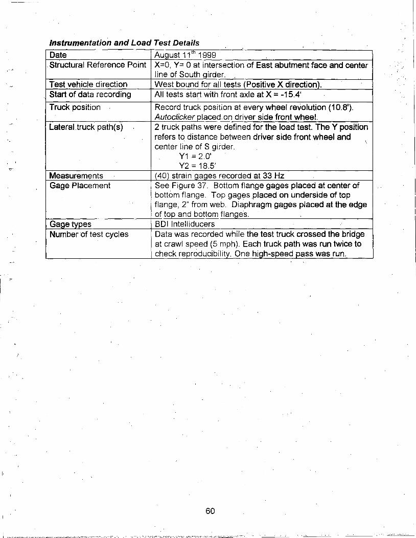
I ,__

i

I


Date August 11th 1999 . Structural Reference Point X=O, Y= Oat intersection of East abutment face and center

line of South girder. Test vehicle direction West bound for all tests (Positive X direction). Start of data recording All tests start with front axle at X = -15.4'

· Truck position Record truck position at every wheel revolution (10.8'). Autoclicker placed on driver side front wheel.

Lateral truck path( s) 2 truck paths were defined for the load test. The Y position refers to distance between driver side front wheel and center line of S girder.

Y1 = 2.0' Y2 = 18.5'

Measurements (40) strain qaqes recorded at 33 Hz Gage. Placement See Figure 37. Bottom flange gages placed at center of

bottom flange. Top gages placed on underside of top flange, 2" from web. Diaphragm gages placed at the edge of top and bottom flanqes.

Gage types BDI lntelliducers Number ·of test cycles Data was recorded whi.le the test truck crossed the bridge

at crawl speed (5 mph). Each truck path was run twice to check reproducibility. One high-speed pass was run.

60

't. SYM. ABOUT

ct ct. ABUTMENT BEARINGS PIER BRIDGE

X=O I I

Y=-0 I 3938 JB71 3940 1-053 Yl=.2' ..... ,..., ,..., .'\ ... :'l.4. 4192 I 417.'\ 1:: l[]:I ~ (,J I I .7'

: :591-B 2372. 4055 I :5916 U) I

. I '"U I 3932 4Ul1 4052 I 3915 ..... t!j I. I • 7'

....... rn I 4111 41 H 4315 I +113 · 3B7B

Y2=18.S' " 41"? 367.3 3933 3872 3935 4115

@ I 575 411 B I • 7'

I 4119 4050 4112 3877 I +120 4057 I Z1Bf Jeeo 4058 I 2139 4:512

- L4.o' - L2· ___r l-.4_0· ---4.0'

4B'...:...g" 48'~9" 62'-6" ..

l'YPICAL GAGE PLACEMENT

'--~ l Il \ N J" .3f-.3B" '1

~-, J CIRDER DIAPHRAGM

Figure 37 IA 3 over East Fork Des Moines River - Instrumentation Plan.

61

6.63K

r-----, ~t- I

I 6.8'

I J_/ -_6_.63_K_

- I

; ..... 13.7'

I !I

9.35K

9.35K

Iii=> i

8.87K

i I I ! I: I I~

I I

6.1'

8.87K

1_l_ I I 11 I

4.4' ~· Figure 38 Load Configuration of Test Truck.

Table 40 Load Test Data Files Truck _ STS Comments Path Data File Y2 DMR1.dat Passenger-side wheels on right shoulder line (missed 1st click). Y2 DMR2.dat Passenger-side wheels on right shoulder line Y2 DMR3.dat II II II

Y1 DMR4.dat Driver-side wheels on left shoulder line Y1 DMRS.dat II II II

Y2 DMR6.dat Passenger-side wheels on right shoulder line High Speed Pass (55 MPH)

Preliminary Investigation of Test Results _

A visual examination of the field data was performed to assess the quality of the data -and to make a qualitative assessment of the bridge's live-load response. Conclusions made directly from the field data were:

• Responses frorn identical truck paths were very reproducible as shown in Figure 39. It is difficult to differentiate between the two passes, indicating nearly identical responses.

• All strain measurements indicated linear-elastic live-load responses. • RC/Steel channel curbs were acting integral.with the superstructure, adding

stiffness_ to the exterior beams. This caused the neutral axis locations of the exterior beams to be considerably higher than predicted by traditional composite analysis. The strain history of an exterior beam at the middle of the center span is shown in Figure 40. Based on this observation, the effective area/depth of the composite concrete block should be increased in subsequent analysis and modeling.

• Analysis of the data from the high-speed pass produced an impact factor of approximately 21 percent. This indicates that the AASHTO (I= 50/(L+125)) Vi:!_l.ue of 22 percent is reasonable. However, since dynamic data was only obtained from a single truck during a singlffhigh-speed pass.it is not likely that the maximum

62

. • . ' •• - =~- • -:: ' • . .• ·:. •. ··· ·.:!,t.~:.v:-_~.'.·_·, .... .-:-::.:"'·~';..:::-:·:·1j:··:.:,·;.;-r~~.;_;..'?·r1 . .- •. \-,::. .. ,::'.~:~··::s·.-:·'-: .~: ··, ·_:___:· ''::__c_-· -_--___::_·· ____:··_:"· ·_::_·-___,_______:___:·-.'---'-'--=·· ··~------'--------------"---------'-'~--

If)

I 0 .._ u

E

z <( 0:: fc.n

impact/dynamic response was measured. An impact factor of 30% is recommended for subsequent ioad rating. Figure 41 shows a comparison of the static and dynamic test data.

STRP.::: lf\JFLUENCE DIAGRAMS SouH' : .<ierio• Beam at her, Poth Y1

10 j···· ................. .

~ 0. 1---------..... t"",°'I!-' ~=----__:::....!;>!:.';;-1"'-.£_ ____ _,_-=!!!!,f"· -~"""""""""'_ ...... _.~--

. \ /' .l -1

-20.

-30.

-4C.

-50.

-6(.

t l y \ . ;:-··· .,... . ············:·····-~f---------------···········-················ -------------------·---

.\ ............. ···; ., ,.

);t: / -... '1~1i~~~~~

' <

: ~ I : ~' ············-v···\··-.~~~-;~-~---~·l:d~-~-~---····························j

~ : "i i:

········1·,··················7·······································;····································

:; ,l' •

......... :~---······ ---~~_./: ..... j------------------------------- --·-···-·················-------------------.\~, ,~it :

......... ~:~t~~t ........ L. ............................. ···········································

. . (, 200. 300 . 400.

(ft.) ....... ~.! .. n.:.:2 ............ . . . - • - . - 4 _1 _ \oJ ;z_: -~. - . - . -

Figure 39 Reproducibility of load test - responses from two identical truck passes.

63

.' · .... - . ·::·;· ·.·

,--.. c 0

~

(fl

I 0

u

E

:z: ::( Q'.: f-Vl

140.

STRAIN INFLUENCE DIAGRAMS South Exterior Beam at Midspan 2. Poth Y1

: : .

120. ··----- ···---------------------------·-------···--······--····-········

100.

80.

60.

40.

·':

20.

0.

-20.

·································································. ········o/ :=~,o~·'·'·'·"''.······································ ""'>,......... )'' r*~·: ~-,'·''fl"; .. ·

·----------··-·····------------------+---···-~'.>:~~~/i$~~;x.<' .. ·:.:. _____________________________________ ; ............. --~~::~;wifr#.~\Yi':<r.~: .......................... ____ _

-40. -100. 0. 100. 200. 300. 400.

TRUCK POSITION (ft.) 4053:3 ----··-------~-} .. ~-~'-~·-··-········

Figure 40 Midspan Exterior Beam Strain Response

,--.. c 0

~

(fl

I 0 '--(.)

E

:z: ::( Q'.: fVl

160.

140.

120.

100.

80.

60.

40.

20.

0.

-20.

-40.

-60.

STRAIN INFLUENCE DIAGRAMS North Exterior Beam. Midspan 2. Path Y2

---·--·------------~---------------------------L ......... . ····>················r\···=::.=····H·i~·h··5·~-;;~·ci-·(·[);~-~~-i-~)···r~-~~-

~---·\,···r···········-------------·'················----·······'············-···-·--·-·--------- ..... -·-· ---------- ---~ ----- --...... --------------~ .......... .

------· ... -- -- ---------- .. -~-------- -------------------~-----. .. . . . . ... --....... -·\· .. ;----------------- ··\·;-----..... ----------- ----- ·t·····. --.......... ·-·· ----~- ........ --............... . Low Speed (S\o\ic)i Poss , ,; \ ~ ,

-··············-----------·r-------------------······--f·---··············,:··· ·r·············----------- · ---·-------··-······--····r···········--·······--·-·t·--····--···-···--------·

I~ :::L zL:~: l\Jy::t I ~:.:;~~

0. 50. 100. 150. 200. 250. 300. 350.

TRUCK POSITION (ft.) 4312: 1 ............. ~,3..1 .. 2.:.~ ............ .

Figure 41 Comparison of Static and Dynamic Loading

64

Analysis and Model Calibration Table 41 provides details regarding the structure model and analysis procedures. A discussion of the analysis results is provided along with conclusions regarding the structural performance.

T bl 41 A I . a e na1ys1s an d d Id t ·1 D M . mo e ea1s- es 01nes R 1ver crossing. Analysis type Linear-elastic finite element - stiffness method. Model geometry Plane grid matching framing plan (see Figure 42) Model components • RC slab represented by quadrilateral plate elements .

• Beam elements corresponding to different sections .

• Curbs simulated by separate beam elements . Live-load 2-D footprint of test truck consisting of 10 vertical point loads.

Truck paths simulated by series of load cases with truck moving , at 10-foot increments.

Dead-load Self-weight of beams, slab, curbs, and parapets with additional 15 psf to account for overlay not included in slab thickness. (Used for load rating only)

Data comparison 40 strain gage locations defined on model (longitudinal beams and diaphragms). Strains computed for 34 truck positions along each path. 40x34x2 = 2720 strain values. Strain records extracted from load test data files corresponding to analysis truck positions.

Model statistics 726 Nodes 1140 Elements 20 Cross-section/Material types 69 Load Cases 40 . Gaoe locations

Adjustable 1 Young's modulus (Ee - ksi) parameters for 2 Exterior beam stiffness - midspan {ly - in4

)

model calibration 3 Exterior beam stiffness - near abµtment {ly - in4)

4 Exterior beam stiffness - near pier (ly - in4)

5 Interior beam stiffness - midspan (ly - in4)

6 Interior beam stiffness - near abutment {ly - in4)

7 Interior beam stiffness - near pier (Iv - in4)

39~~J==l~=t=~~~~~~~~=t===*=~~~~=P~~:f'=P:::pqt::q=f~~~~ 39

39 : 4055: 39~~~~-t--~--+--t----crtrn-r~~~:~I -t---~-!--n!=-1~>-t-~--t---r---t--t--r-1~----t----f71~...,_--1-I

Figure 42 Finite Element Mesh - Des Moines River.

65

• • • ~ ,, 'j ', ·\ •

A model with the above parameters was defined and the analysis program simulated the load test process. The accuracy of the model was defined by comparing the 2720 computed and measured .strain values. Selected parameters were modified to minimize the comparison, error. · ·

Typically, all bridges show some level of moment resistance at the supports, making it necessary to include rotational or longitudinal springs in their respective models. The data from this bridge, however, indicated negligible moment restraint at the abutments and piers. Considering this and the rocker support conditions at both locations, no support moment restraint was added_ to the model. · ·

Table 42 contains the original stiffness parameters and the final values after the model calibration process. Statistical accuracy· values associated with the initial and final models are-provided in Table 43. The resulting accuracy terms were in the typical

. range for steel structures. · ·


Deck modulus E ksi . 3,600 5,775 Exterior beam - midspan (I) In" 40,982 47,530 Exterior beam - near abutment (I) In" ' 36,354 42, 160 Exterior beam - near pier (I) In" 70,055 81,250 Interior beam - midspan (I) In" 52,775 56,500 Interior beam - near abutment (I) In" 44,973 . 48,150 Interior beam - near pier (I} In" . '71,338 76,380


Absolute Error 5359.8ua · 2546.6ua Percent Error 8.2% 2.0% Scale Error 10.4% 3.2% Correlation Coefficient 0.98 0.99


Load rating factors were computed for the longitudinal beams using the_ Load Factor method. A Load Factor of 1.3 was applied to all dead-load affects for both Inventory and Operating load ratings, while load factors 2.17 and 1.3 were applied to live-load responses. Ultimate strength member capacities were computed, based on AASHTO specifications for steel beams, except that inoment capacities were limited to yield stress of the extreme fiber rather than plastic moment capacities. Positive moment capacities were obtained for midspan cross-sections, negative moment capacities were computed for cross-sections at the piers, and shear capacities were calculated for the sections at the abutments and piers.

The modeling and calibration phase of the analysis yielded neutral axis values for the beams near the piers that indicated composite behavior even _in negative moment.

66

However, for rating purposes, the beam cross sections iri negative moment regions were computed as non-composite sections. Also,_ the majority of dead load was applied to a non-composite model. The non-composite dead-load stresses were subtracted from the original yield stress, at each crit'ical section, to obtain composite member capacities. A yield stress of 35 ksi was assumed, based on the provided mill test · reports. Table 8 contains the resulting· moment and shear capacities for the composite model.

T bl 44 Ulf t t a e 1ma es reng th t T i b momen capac1 1es or f earn sec tons. . '

Member Ultimate Strenoth Capacity . Moment (K in) Shear (Kips)

Exterior Beam Midspan (Span 1) 35,292 N/C Midspan (Span 2) · 36,639 N/C Near Abutment N/C 528 Near Pier -39,338 .528

Interior Beam Midspan (Span 1) 44,408 N/C Midspan (Span 2) 46,082 N/C Near Abutment N/C 542 Near Pier -49,451 542

Load rating calculations were performed for the HS-20 and the three Iowa rating vehicles by applying the truck configurations. to the calibrated model. Due to the width of the roadway, two truck paths were defined. The first path was defined by placing a wheel line 2 feet from the face of the curb. The second truck path was defined as being 12 feet from the first path. Single lane loading envelopes (critical responses) were generated for every model component by moving the applied rating truck at 8-foot intervals along the length of the bridge. Multiple lane load conditions were obtained by the principle of superposition. The response envelopes were added to generate twolane loading response envelopes.

Dead load responses were obtained by applying 22 PSF to account for concrete overlay not included in the deck model components and the railing. Note that the noncomposit~ dead-load effects were subtracted from the member capacities prior to running the rating analyses. Table 9 contains computed dead ·load and the various rating vehicle live-load forces for each critical beam section. Inventory and operating rating factors for each component are listed in Table 46.

67

··~ ;.":•'• •.-~:.:•.•;.-;-;..,-··.~ .,_ .. ~,.!.."''·•._;V·.•!.•'.• ,, ~:".'''1") •. ,.•.'• '•:• • '

Table 45 Dead load and maximum live load forces on critical beam sections. Member Units Dead- HS-20 Type4 Type 3-3 Type·

' Load* 3S3 Exterior Beam

Mid - (Span 1) Mom. Kin 1,102 8,446 6,861 8,216 8;059 Mid - (Span 2) Mom. Kin 1,241 8,882' 7,104 8,668 8,478 Abutment Shear Kips 35.6 33.8. 26.0 31.3 31.5 Pier Moment Kin -5,632 -5,377 -4,134 -5,(377 -5,632 Pier. Shear Kips ·62.0 35.8 28.4 35.8 35.5

Interior Beam Mid - (Span 1) Mom. Kin 1,357 8,769 7,282 8,405 8,249 Mid - (Span 2) Mom. Kin 1,502 9,242 7,510 8,830 8,590 Abutment Shear Kips 45.1 37.4 28.8 33.9 34.5 Pier Moment Kin -5,978 -5,696. -4,370 -6,028 5,978 .Pier Shear Kips 83.8 40.1 . 32.3 '39.3 39.4

* Composite dead-load only ".' non-composite dead-load effects subtracted from member capacities.

..

T bl 46 L d R f F t a e oa a rng ac ors- D M. es ornes R 1ver. Member HS-20 Type4 Type 3-3 Type 383

Inv .. .

Oper . Inv. Oper. Inv. Oper. Inv. Oper. Exterior Beam ' .

Midspan 1 Mom. 1.41 2.36 1.75 2.92 1.46 2.44. 1.49 2.49 Midspan 2 Mom. 1.40 2.33 1.75 ·. 2.92 1.43 2.39. 1.46 2.44 Abutment Shear ·5_06 8.45 6.58 10.98 5.45 9.10 . 5.42 9.04' Pier Moment .2.43 4.05 3.16 5.27 2.30 3.84 2.32 3.87 Pier Shear 4.43 7.39. 5.61 9.37 4.43 7.40 4.47 7.46

Interior Beam Midspan 1 Mom. 1.71 2.85 2.08 3.47 1.80 3.00 1.83 3.06 Midspan 2 Mom. 1.69 2.83 '2.08 3.48 1.77 2.96 1.82 3.04 Abutment Shear 4.58 7.65 5.94 9.92 5.06 8.45 4.97 8.29 Pier Moment 2.87 4.78 3.73 6.23 2.71 4.52 2.73 4.56 Pier Shear 3.81 6.36 4.76' 7.94 3.89 6.49 3.90 6.50

Critical RF 1.40 2.33 1.75 2.92 1.43 2.39 1.46 2.44

Conclusions and Recommendations The analysis results from the initial model were reasonably accurate, indicating that the · structure is behaving in a normal manner.· The slight modifications to model parameters to improve the comparison with measured strains included a 7% increase in interior beam stiffness, 15% stiffness increase in the exterior beams, and a substantial increase in the effective deck stiffness. The resulting deck modulus should not be considered accurate from a material standpoint. The transyerse crown of the deck improved the lateral distribution properties of the deck. This geometr-Y effect was compensated for, in the plane model, by increasing the effective deck stiffness.

68

The structure exhibited relatively large dynamic effects compared to the shorter bridges that were tested. The measured dynamic response of 21 % was approximately equal to

· the factor computed from the AASHTO impact formula. However, only a single highspeed truck pass was .recorded. It is likely that different vehicle speeds and different trucks could induce greater dynamic responses. Therefore, an impad factor of 30% was applied to the live-load for all load-rating calculations.

The load rating factors presented in this report are based on the structure's condition at the time of load testing. Any structural degradation must be considered in future load ratings. Note that no ~ffort was made to assess the condition or capacity of the substructure elements such as the abutments or piers.

I ,

69

"•.'•r·,.-.t'.":'":"• ··:·:·

Bridge 9951 .4S003 Eagle Creek- Steel and PS/Concrete Beams


Structure Identification 9951.4S003 Location IA 3 Over Eagle Creek -Wright County Structure Type Single Span, Widened structure

Original: Steel Beams Widened Section: Prestressed Concrete Beams

Span Length(s) Original: 40'-0" Widened Section: 40'-0" up to 52'-0" (@ Exterior beams

Beam Spaces 10 spaces at 4'-3 1 /4" Skew Perpendicular Structure/Roadway Widths Original: 28'-0" I 24'-0"

Widened : 46'-6" I 44'-0" Curb/Parapet Detail RC curb integral with slab and RC parapet Visual condition Beams in good condition with minimal corrosion and loss

of section .

70


Date August 12tn 1999 Structural Reference Point ·x=o, Y= 0 at intersection of West abutment face and !

center line of South exterior PS/C girder. Test vehicle direction East bound for all tests (Positive X direction). Start of data recording All tests start with front axle at X = -15.4'

Truck position Record truck position at every wheel revolution;(10.8'). Autoclicker placed on driver side front wheel.

Lateral truck path(s) 4 truck paths were defined for the load test. The Y position refers to distance between driver side front wheel and centerline of S girder: Y1=10.0' Y2=16.8'. Y3 = 33.5' Y4 = 40.3'

Measurements (40) strain gages recorded at 33 Hz Gage Placement See Figure 43. Bottom flange gages placed at. center of

bottom flange. For steel· beams; top gages placed on underside of Jop flange, 2" from web. For concrete beams, top gages placed on side of top flange.

Gage types BDI lntelliducers Number of test cycles · Data was recorded while the test truck crossed the bridge

at crawl speed (5 mph). Each truck path was run twice to check reproducibility. One high-speed (50 mph) pass was also run along path Y2.

'----------sa·-o·---------'

Figure 43 IA 3 over Eagle Creek - Instrumentation Plan.

71

6.63K 9.35K 8.87K

I I I II 11 I I

6.8' 6.1'

j_I 9.35K 8.87K

,J_ 6.63K I I I I I 11 I

~ 13.7' ~ 4.4' ~ Figure 44 Load Configuration of Test Truck.

Table 47 Load Test Data Files Truck STS Comments Path Data File Y1 EAGLE1.dat Driver-side wheels on right shoulder line Y1 EAGLE2.dat II II II

Y1 EAGLE3.dat Passenger-side wheels on right shoulder line Y1 EAGLE4.dat II II II

Y2 EAGLE5.dat Driver-side wheels on left shoulder line Y2 EAGLE6.dat II II II

Y2 EAGLE7.dat Passenger-side wheels on left shoulder line Y2 EAGLEB.dat II II II

Y1 EAGLE9.dat Passenger-side wheels on right shoulder line High Speed Pass (50 MPH)


• Responses from identical truck paths were very reproducible as shown in Figure 45. • The majority of strain measureme,nts indicated linear-elastic live-load responses.

All gages returned to the zero point when the truck drove off of the bridge. • Contrary to the non-composite design, the steel beams all exhibited composite

behavior, as shown in Figure 46. • Because the beams were embedded in concrete at the supports, the torsional

stiffness of the abutment had an effect on the gages located near the end of the beams. This produced positive moment responses instead of the expected negative moment (due to the rotational restraint) when the truck was far away from the beam. Figure 47 shows a typical strain history of a gage pair located near to an abutment.

• Analysis of the data from the high-speed pass produced an impact factor of approximately 20 percent. This proves the AASHTO value of 30 percent to be conservative. Figure 48 shows a comparison of the static and dynamic test data.

72

,-... c D ..._ ~

en I

0 ..._ u

E

5a.

4a.

3a.

;rn.

1 a.

a.

-1a. -15. -5.

4057:1

STRAIN INFLUENCE DIAGRAMS Midspan Steel Beam, Path Y1

5. 15. 25. 35. 45.

TRUCK POSITION (ft.)

55. 65.

---·····-·---~.Q.~.?.:X ... ________ _

75.

Figure 45 Reproducibility of load test

,..--..-. c D

~

en I

0

u

E

:z <( O'.'. l-e(/)

40.

STRAIN INFLUENCE DIAGRAMS Midspan Exterior PS/C Beam, Path Y1

30. ··-···-·----------1---···------------·:--·------------··r·-----····---·--~--··-·······--,:.::;tP!'.-\.};·1..\r---·--········-+················+·················.-················· ! Bottom Flong~ ""' i (i'.i i · :;<, . '

" . ! 20.

10.

-10. -15. -5. 5. 15. 25. 35. 45. 55. 65. 75.

TRUCK POSITION (ft.)

85.

85.

4115: 1 ------·······~.! .. 1--~'-~------···---- ··-------·--).9._Ui.:.! ............. . . -- . ---~_El_:!_ 6_:!2_ ·-. -· -

Figure 46 Composite Behavior of Steel Beams

73

.--.... c:

0

(J)

I 0 I....

u

E ..___..

:z <( 0::: t-(/]

10.

B.

6.

4.

2.

0.

-2.

-4.

STRAIN INFLUENCE DIAGRAMS Interior Steel Beam, Path Y3 Near Abutment

:~Jr··-·i r~

T -r '. ;tl :"\t 1 ! r : Bottom Flange : :' : . ;11:.. ; ; ; .

- : t-~71 lj\+ + -,

~ r ;;;F:~:~~r I I >1;;:~-i:,w~[L l : 1:: :i:::, :i "'·+·----·-.. : ''""·wr wr .. ::: : "' ·::.~

-+ r;~;;;g;~J j + I + -1 o. a. 1 o. 2a. 30. 40. 50. 60. 70. so.

TRUCK POSITION (ft.) 3873 ............... ~.9.?..~ .............. .

Figure 47 Strain History of Steel Beam Near Abutment

c 0

(J)

I 0 ...... u

E

120.

100.

80.

60.

40.

20.

0.

-20.

STRAIN INFLUENCE DIAGRAMS Midspan Interior Beam, Path Y2

~,;~~,~:;;~D;;:~,:)~:-~;=:zr\::[ :; l - , l ! ! I I : I ! '

r 1

I-:: v : r -\J f ~;;~,;;1::;~,'.:::;~'.;;r .. ................................ r ......... :.:.t .. ( ................................... ~ ................. r .. ·"~; ..........

1

................. , ................ -r ................ , ................ . -~-- .1 ... ____ ,. "\

•:.

-10. 0. 10. 20. 0. 0. 5a. 60. 70. BO. 90. 1 00.

TRUCK POSITION (ft.) 4057: 1 ............. '.!.9.?..Z.:.;? ............ .

Figure 48 Comparison of Static and Dynamic Loading

74

Analysis and Model Calibration Table 48 provides details regarding the structure model and analysi~ procedures. A discussion of the analysis results is provided along with conclusions regarding the structural performance.

T bl 48A I . a e na1ys1s an d d I d t ·1 E I C k mo e e a1s- age ree crossing. Analysis type Linear-elastic finite element - stiffness method. Model oeometrv Plane grid matching framing plan (see Figure 42) Model components • RC. slab represented by quadrilateral plate elements .

• Beam elements corresponding to different sections . Live-load ' 2-D footprint of test truck consisting of 1 O vertical point loads.

Truck paths simulated by series of load cases with truck moving at 10-foot increments.

Dead-load Self-weight of.beams, slab, curbs, and parapet~' with additional 15 psf to account for overlay not included in slab thickness. (Used for load rating only)

Data comparison 21 strain gage locations defined on model (longitudinal beams). Strains computed for 13 truck positions along each path. 21x13x4 = 1092 strain values. Strain records extracted from load test data files corresponding to analysis truck positions.

Model statistics 202 Nodes 393 Elements 11 Cross-section/Material types 52 Load Gases 21 Gage locations

Adjustable 1 Young's modulus of concrete for both original and widened parameters for sections (Ee - ksi) model calibration 2 Steel ·beam stiffness (ly - in4

)

3 Exterior PS/C beam stiffness (Iv - in4) I

4 Interior PS/C beam stiffness (Iv - in4)

5 Rotational end.,.restraint for steel and PS/C beams (k-in/in)

75

-.... .... \~ (

.. \ .. ... "II,,, "Ill"

... ... ....... 'I!.,, "I II"

..... .il!I..

" ., "II iJ'

... i. All. .. .,, .. it"

.... • ;a,.

" II' ... .,

... ~ .. "" .. .,, .. ill"

.... .a :..

... /" ...

~ J!ll" ~ '"¥' - -

Figure 49 Finite Element Mesh - Eagle Creek

A model with the above parameters was defined and the analysis program simulated the load test process. The accuracy of the model was defined by comparing the 1092 computed and measured strain values. Selected parameters were modified to minimize the comparison error.

The ends of the beams were embedded in the concrete abutments, producing significant end restraints. This was simulated by adding rotational springs to the model and then optimizing their stiffness to best match the test data. The resulting concrete stiffnesses varied considerably between the original slab and the new slab. The modulus values are not considered to realistic values for the concrete itself. Rather they are the effect modulus values for flexure. The lower modulus of the original slab indicates that it is a higher degree of flexural cracking, additionally the effective span lengths are greater due to the differences in beam flange widths. '

Table 49 contains the original stiffness parameters and the final values after the model calibration process. Statistical accuracy values associated with the initial and final models are provided in Table 50.

76

.. : ·.· .. · ...

T bl 49 Ad. t bl P a e IJUS a e t R It arame er esu s. Stiffness Parameter Units· Initial Value Final Value

Original slab modulus E ksi 3,600 1,325 Widened slab modulus E ksi

I

3,600 3,400 Steel beam Clv} - composite ln4 9,917 8,800 Exterior PS/C beam (Iv} ln4 106,309 212,180 Interior PS/C beam (Iv} ln4 106,309 142,840 Rotational end restraint - PS/C bms K-ln/rad 0 648,380 Rotational end restraint - steel bms k-in/rad 0 495,030

T bl SOM d IA a e o e ccuracy Statistical Term Initial Value Final Value

Absolute Error 5079.4UB 16Q1.4UB Percent Error 32.4% 3.4% Scale Error 14.1% 3.5% Correlation Coefficient 0.86 0.98

Load Rating Calculations Load rating factors were computed for the longitudinal beams using the Load Factor method. A Load Factor of 1.3 was applied to .all dead-load affects, while load factors 2.17 and 1.3 were applied to live-load responses for Inventory and Operating load ratings, respectively. Ultimate strength member capacities were computed, based on AASHTO specifications for steel beams. Positive moment capacities were obtained for , midspan cross-sections and shear capacities were calculated for the sections near the face of the abutments.

Although the plans do not indicate that the bridge was designed to rely on composite, behavior between the steel beams and the concrete deck, the field data shows that all beams acted compositely. Subsequently, the bridge was rated using the load.factor method with the beam capacities being limited by yield stress of the composite sections.

A recommended means of checking the reliability of this unintended composite strength is to calculate the shear forces along the interface of the steel beam and the concrete deck using allowable stress parameters. A.G. Lichtenstein and Associates, Inc have suggested a horizontal shear stress of 100 psi as a reasonable limit for unintended composite action. The maximum calculated shear force, for HS-20 loading plus impact, was approximately 30% higher than the accepted value. However, the construction

. details show that any slippage of the interface is very unlikely. For this reason, the rating was performed on a model consisting of composite sections for both concrete and steel beams. Table 51 contains moment and shear capacity values for both steel and PS/C beam sections. The moment capacities were computed using non-composite action for dead load contribution, and composite action for positive live load moments.

77

T bl 5 UI. t t th ' '' T f b a e 1 t1ma e s reng· capac1 1es or earn sections. Member Ultimate Strength Capacity

Moment CK in) Shear (Kips} Steel Beams 9,057 223 PS/C Beams

Exterior 9,770 105 Interior ,10,087 114

Load rating calculations were performed for the HS-20 arid the three Iowa rating vehicles by applying the truck configurations to the calibrated model. Due to the width of the roadway, three truck paths were defined. The first path was defined by placing a wheel line 2 feet from the face of the curb. The second arid third truck paths were defined as being 12 feet from the· previous paths. One of the three paths also provided critical loading for the interior steel beams. Single lane loading envelopes (critical responses) were generated for every model component by moving the applied rating truck at 2-foot intervals along the length of the bridge. Multiple lane load conditions were obtained by the principle of superposition. The response envelopes were added to generate two and three-lane loading response envelppes.

Dead load responses were obtained by computing the self-weight of the structure. The non-composite dead-load effects were subtracted from the mem.b~r capacities prior to load rating. An additional 25 PSF was applied to the composite model to account for concrete overlay and guardrails . .Table 52 contains computed dea_d-load and the various rating vehicle live-load forces for each critical beam section. Inventory and operating rating factors foreach component are listed in Table 53.

Table 52 Dead load and maximum live load forces on critical beam sections. . Member Units Dead-Load HS-20 Type4 Type 3-3 Type 3S3

Steel Beam Moment Kin 1,710 1,334 1,169 976 1,097 Shear Kips 18.9 22.0 17.7 16.9 17.1

Exterior PS/C Beam Moment Kin 3,099 1,994 1,730 1,619 1,556 Shear· Kips 19.1 14.0 10.8 11.6 13.4

Interior PS/C Beam .. Moment Kin 2,782' 2,017 1,783 ·1,578 1,607 Shear Kips 9.3 ' 16.2 13.1 ·12.2 12.5

78

/

·!

I

T b 53 L d R f F ct E I C k ' ' . ~ .

a le oa a ing a ors,;_ age ree . Member HS.,.20 Type4 Type 3-3 Type 3S3

Inv. Oper. Inv. Oper. Inv. Oper. Inv. Oper. Steel Beam

Moment 2.31 3.86 2.64 4.41 3.16 5.28 2.81 4.70 Shear 3.53 5.89 4.37 7.29. 4~57 7.63 4.52 7.55

Exterior PS/C Beam Moment 1.62 2.71 1.87 3.12 2.00 3.33 2.08 3.48 Shear 2.55. 4.25 3.30 5.51 3.06 5.10 3.13 5.23

Interior PS/C Beam Moment 1.67 2.79 1.89 1 3.16 2.14 3.57 2.10 3.50 Shear 2.42 4.04 2.98 4.98 3.20 5.34 3.14 5.24

· Critical RF . 1.62. 2.71 1.87· 3.12 2.00 3.33 2.08 3.48

Conclusions and Recommendations Load rating factors for the steel beams are relatively high - to the extent that the controlling factor is the moment capacity of the exterior PS/C beams. The rating for the interior steel beams relies on two performance factors that were observed during the load test. First it was observed that the beams acted compositely with the RC deck even though the plans did not indicate any shear connectors. Due to· the construction details and redundancy of the structure, it was determined that composite action was reasonab_le for rating purposes. The ·second observation was relatively fixed endconditions provided by the embedded beam supports. The supports have the effect of significantly reducing midspan moments.

The condition of the end-diaphragm (beam supports) and the beam"-deck interface should be examined thoroughly during future inspections to validate the rating assumptions provided here. 1

The load rating factors presented in this report are based on the structure's condition at the time of load testing. Any structural degradation must be considered in future load ratings. Note that no .effort was made to assess the condition or capacity of the substructure elements such as the abutments or piers.

79

I ··:: ..... .,__ .. _:-.. :·~·:··!·:··,· :;·-.::.: .. :.:·:_:·.:-:-:.!·";~~.i:.;·z'!··:-::~"',:;~·7~··: ·:~:?-'. .. -:<'.·;:::::?. :· ~- ~-····'·--; ~,_. · · " :.~- ·:·· :-_ ·

Bridge 9712.1 R020 Elliot Creek - Parabolic RC T-beam


Structure Identification 9712 .1 R020 Location Us-20 over Elliot Creek - Woodbury County Structure Type 3 span continuous RC t-beams.

Variable depth beams (parabolic profile) Span Lengths 44'-6", 61'-0", 44'-6" Beam Spaces 9'-9 1/2", 10'-1 1/2", 9'-9 1/2" c.c. Skew Perpendicular Structure/Roadway Widths 34'-8" I 28'-0" Curb/Parapet Detail RC curb integral with exterior beam and deck.

RC parapet/guardrail directly above exterior beam web -not part of original structure. Parapet is continuous and no sign of distress.

Visual condition Beams in good condition with minimal cracks. No spalling of concrete or exposed reinforcement.

80


Date Structural Reference Point Test vehicle direction Start of data recording

Truck position

Latera'I truck path( s)



ct ABUThlENT BE:>RINGS

August 3ra, 1999 X=O, Y= 0 at Southwest abutment beam bearing .. East bound for all tests (positive X direction) ... All tests.start with front axle at X = -15.4'

.Record truck position at every wheel revolution (10.8'). Autoclicker placed on driver side front wheel. 2 truck paths were defined for the load test. The Y position refers to distance between driver side front wheel and centerline of south girder.

Y1 = 10.5' Y2:: 26.4'. I

(36) strain gaoes recorded at 33 Hz See Figure 43. Bottom beam gages placed at center c;if web. Upper beam gages located below bevel. Distance between gaQes varies. BDI lntelliducers with 18" extensions (21" gage length) Data was recorded while the test truck crossed the bridge at crawl speed (5 mph). Each truck path was run twice to check reproducibility. One high-speed (45 mph) pass was also run along path Y2.

t. er. E!RJOOE PIER

Figure 50 US-20 over Elliot Creek - Instrumentation Plan.

81

6.SOK 9.60K 8.10K

I I I Ti I I 1-i-I

6.9' ' ' 6.0'

l_ 7.85K · 8.9.SK

1_l 7.35K I I I I I I 11 I

·~ 13.9' ~ 4.5' ~


Table 54 Load Test Data Files Truck STS Comments Path Data File Y1 ELLIOT1 .DAT Passenger side wheel on south shoulder line - slow Y1 ELLIOT2. DAT Passenger side wheel on south shoulder line - slow Y2 ELLIOT3.DAT Driver side wheel on north shoulder line - slow Y2 ELLIOT 4. DAT Driver side wheel ori north shoulder line - slow Y2 ELLIOT5. DAT . Driver side wheel on north shoulder line - fast 45 MPH


• All responses were linear-elastic. Strains from all transducers returned to zero after each truck crossing.

• Reproducibility of data from identical truck passes was excellent a~ shown in Figure 52. .

• Neutral axis measurements on exterior beam sections consistently higher than calculated for section consisting of web, .deck and curb only. Indicates RC guardrail is contributing to stiffness of exterior beam. Figure 53 shows strains from upper and lower gages at midspan of southern exterior beam. Strains from both gages have the same sign indicating neutral axis weli above upper gage position.

• Interior beam responses had a high degree of symmetry with the symmetrical load conditions as shown in Figure 54. Exterior beams were reasonably symmetric but not as consistent as the interior beams. This could be an indication that the exterior beams have a higher density of tension cracks in the concrete.

82

L '-~- ~-:_·_:.c··:_:_·· :-.._:____:_~__:_---------~-·~· .. .....;' .. _ ___. ___________________ _

(/)

I 0 "u

E

:z <( 0::: tUl

90.

80.

70.

60.

50.

40.

30.

20.

10.

0.

-10.

-20.

STRAIN INFLUENCE DIAGRAMS MIDSPAN INTERIOR BEAM - SPAN 2 - 2 PASSES @ Y1

. . . i i ---+---- PASS! 1 @ Y1

···········-·--·······-~---····················1·······-··············+·-·············--···-!---····· .. ::.: --~---·pA·s~··2··©··yr·····..; ..................... ..

.. ..................... L ..................... ) ...................... + ..................... L .................. : ....................... .L. ................... ; ..................... ..

·······················!·······················'······················' t············· 1·····················i·····················'·······················

. ...................... : ....................... ; ....................... ; ................ ' ---r ................... ··+ ...................... -f ...................... .; ...................... .

·······················1··················· .... ! ....................... , .............. T, ........... L .............. : ...................... . ....................... : ....................... ! ....................... ; ...................... ]' ....................... ~ ...................... ; ....................... ; ..................... .. ·······················1·······················i············-········;····················' T ................ : ................ , ..... . .............................................. \ ....................... ~-· .................... L. ..................... , ......... .

,,-···

0. 20. 40. 60. 80. 100. 120. 140. 160

TRUCK POSITION (ft.) 3940: 1 ............. ~.~:~.9.:.? ............ .

Figure 52 Reproducibility of strain responses - midspan Span 2.

(/)

1. 0

E

:z <( 0::: tUl

60.

50.

40.

30.

20.

1 o.

STRAIN INFLUENCE DIAGRAMS MIDSPAN EXTERIOR BEAM UPPER AND LOWER GAGES

--·-----------·-·····- --·1········---·-·······-··-~----. .:'· .......... :\. BQTTOM WEB GAGE

l:/ ----······------·-····--·-········ ------~_:.:~·-: . ··········--········--- ········----······· --····· ----·········---

': l

. -· ----- ... ----. -----··'--- ---......... --. -... -~------------------- ----~------- ........ £. --... -~--. --- ......... . ........... --- ....... -------· .• -- -- -- ..... . : -- - .· ..

........ ,_

'"·-.~-... ..... " - 1 0. . ...................... 1 ... :-. . .,_.::.::~·-::::::.:::t:~:-'-~-< ............ , ........................ ~-···· ................. , ..................... : .. : ...... .

• •·-, •• ,,..., ~-~· r

-20. o. 20. 40. 60. 80. 100. 120. 1 40.

TRUCK POSITION (ft.) 4111: 1 ............. <\ .. ~.1.) ... ~ ........... .

Figure 53 Strain histories indicating contribution of guardrail to exterior beam.

83

1 60.

STRAIN INFLUENCE DIAGRAMS . SYMMETRY OF RESPONSES @ INTERIOR BEAMS SPAN 2

90.

80.

. . . . . --+- soyrn INT. BEAM @ PASS y ---------·-------------·-----------------------~------------------------:---------------------~--~------- S.-··· -------;-----------------------;-----·····--·-······----:------------------------

: : ! ! .\ : NO~TH INT. BEAM @ PASS 70.

: : : : ~ : : : ·----·----------·-·-··-r·················--···<·----·······-·· .. -----··r··----·-·········------:-····· ... ····· .. ":····-·:··--------·············· ... -····················r······· .. ·············

-------60.

c 0 ~ 50. ~

(/)

I 0 40. ~

u

E 30. -----:z: <( 20. O'.:: r-(/) 10.

-----------------------~-----------------------+----------------------+----------------------+--- -------------~ ----~-----------------------~----------------·-·----~-----·-·····-----······· . : : > : . . : : : / . ' . . --------------------·-·r··-----------------·-·r···-------------------1··------------· :.\.: .... ~--------············\ ··1········ ····--······--1··~---···-·------·-····T······-·--------······-

i i . . \ i SOUT~ INT. BEAM ~ PASS Y2 ---- ---------·--------·I--------------·-·------~---------------------- ·-r·· -··-------- -----·--r-~.~~;:~~~;;~~~:······ \ · ····----- ·--------·····r· -----------------· ·· ·r· · ·· · · ···· · -·- ---------

! . ! .;:-.~- . ·'">\. ; NOR11!i INT BEAM !@ PASS Y1

:•···············••1. l 1>''.~'.} :···;,.. '· ; . ~

-10.

-20. '---'-~~--'-~~_.._~~~-.~~-'-'~~~~~~--'-~~~"--'"~~

0. 20. 40. .60. 80. 100. 120. 1 40. 160.

TRUCK POSITION (ft.) 3940: 1 ............ }.9..'7.Q:.~ ............ . ............. ~.9..~!?.;.! ... , ......... . .. - . - --~.9.~9~ 2 ___ . - . -

Figure 54 Symmetry of interior beam strains at midspan of span 2.

Analysis and Model Calibration Table 5 provides details regarding the structure model and analysis procedures. A discussion of the analysis results is provided along with conclusions regarding the structural performance.

Table 55 Anal sis and model details - Elliot Creek. Linear-elastic finite element - stiffness method. Plane rid matchin structure framin Ian see Fi ure 6 .

Model components • Prismatic beam elements representing beam sections 1 /1 ih span length in end-spans and 1 /1 Bth span length at middle span. Properties for each beam segment were based on average depth of beam segment. Figure 56 shows the depth ofeach beam segment relative to the bridge centerline. Actual beam depths vary due to crown of bridge deck.

• Prismatic beam elements representing transverse .diaphragms. ·

• Quadrilateral plate elements representing deck - 3 plate elements between each beam.

Live-load 2-D footprint of test truck consisting of. 1 O vertical point loads. Truck paths simulated. by series of load cases with truck moving at 5-foot increments. ·

84

Dead-load Self-weight of slab, curbs, and parapets with additional. 15. psf to . account for overlay not included in slab thickness. (Used for load rating only) \

Data comparison 18 longitudinal strain gage locations defined on model (bottom of T-beams). Strains computed for 29 truck positions along each path. 29x18x2 = 1044 strain values. Strain records extraeted from load test data files corresponding to analysis truck positions ..

Model statistics 430 Nodes 634 Elements 50 Cross-section/Material types 58 Load Cases 18 Gage locations

Adjustable 1 Young's modulus - span 1 Int. beam+ moment (Ee - ksi) parameters. for 2 Young's modulus - Int. beam near piers - moment (Ee - ksi) model calibration 3 Young's modulus - span 2 int. beam+ moment (Ee - ksi)

4 Young's modulus - span 1 Ext. beam+ moment (Ee - ksi) I 5 Young's modulus - Ext. beam near piers - moment (Ee - ksi) ·

6 Young's modulus - span 2 Ext. beam+ moment (Ee~ ksi) · 7 Young's modulus - regions of low moment (no cracks) (Ee - ksi)

Figure 55 Finite el~ment mesh of bridge.

top of cieck a. t bricige centerline ~ bottDl"'l of bea.M web

1 2 3 4 5 7 8 9 10 11 12 13 14 15 16 17 18 19 20 21

[\) f\) ru [\)

I\) ru N ru ru ru N w w w· -I> -I> -I> w w w \D 9=l ~ ~· -...J w ...... Ui Ul Ul °' -...J -...J CD CD Cl w CJ'\

,_. CD CD w ::...i .b (]'\ ,_. Cl .

iu en ~ b Ui ·. t=- ~ ~ ;..... fu iu iu °' Cl o:J ru N -I> \Cl °' w a o:J Ul ,_. -I>

,_. ,_. CD \Cl N CD Ul

Figure 56 Depth profile of parabolic beams.

A model with the above parameters was defined and the analysis program simulated the load test process. The accuracy of the model was defined by comparing the 1044 computed and measured strain values. Selected paramet~rs were modified to minimize the comparison error.

85

."_.- ....... ,· ..

The general conclusions were that.the RC guardrails did in fact contribute to the exterior beam stiffness.· Beam cross-sections in the immediate vicinity of the piers and at midspan of Span 2 had stiffness below the .gross concrete section indicating the presence of concrete tension cracks.

Table 56 contains the original stiffness parameters and the final values after the model calibration process. Statistical accuracy values associated with the initial and final models are provided in Table 57. The resulting accuracy terms were exceptionally good for RC slab structures. The relatively high accuracy is an indication that the bridge responses are very linear and that the measurements were not heavily influenced by flexural cracks in the concrete.


Int. Bm Span 1 +M Ee ksi 3200 3246 Int. Bm Pier -M Ee ksi '3200 2436 Int. Bm Span 2+M Ee ksi 3200 . 2229 Int. Bm Span 1 +M Ee ksi 3200 3600 Int. Bm Pier -M Ee ksi 3200 2667 Int. Bm Span 2+M Ee ksi 3200 2208 Low Moment Ee ksi 3200 3600.

T bl 57 M d I A a e o e- ccuracy Statistical Term Initial Value Final Value

Absolute Error 5578 UE 1258 µE Percent Error 27.4% 2.5% Scale Error 8.7% 1.7% Correlation Coefficient .92" .99

Load Rating Calculations · Load rating factors were computed for the structural components of the superstructure · using the Load Factor method. A Load Factor of 1.3 was applied to all dead-load affects for both Inventory and Operating load ratings, while load factors 2.17 and 1.3 were applied to live-load responses. Ultimate strength member capacities, based on AASHTO specifications for reinforced concrete beams, were computed for positive and negative moment regions and shear near the supports. Positive moment capacities were obtained for several cross-sections near midspan and negative moment capacities were computed at noda.1 locations· near the piers and abutments.

Since the guardrails were effective in load distribution, the additional concrete was -included in the shear capacity and pos'itive moment capacity of the exterior beams. Since the amount of steel in the parapets was unknown, it was assumed that they would not contribute to the negative moment capacity.

Table 58 contains shear and moment capacity calculations for various critical beam sections. Grade 40 reinforcement, with a mini_mum yield stress of 40 ksi, was assumed

86

:: ·:·\' · ... ·· .. ~. . .

based on the age of the structure. A concrete strength of 4 ksi was allowed due the relatively high concrete modulus obtqined from the model ·calibration process.

T bl 58 Ult" t t a e 1ma es reng th T f b capac1 1es or r earn .cross..:sec ions. Member Ultimate Strength Capacity

Moment (Kin) 1 Shear (Kips) Interior Beam Sections

lnt-1 (abutment) - 143 lnt-2 - 147 lnt-3 16170 173 lnt-4 18390 -lnt-5 18910 -

· 1nt-6 19430 -lnt-7 18120 -lnt-8 12060 -lnt-1 O -20890. -lnt-11 -· -27840 173 lnt-12 adjacent to pier -33910 202 lnt-13 adjacent to pier -34200 210 lnt-14 -28360 209

-lnt-15 -21770 -lnt-20 - 19400 -lnt-21 (midspan 2) 19330 -

Exterior Beam Sections Ext-1 (abutment) - ss-Ext-2 - 99-Ext-3 1181 O* -Ext-4 11940* -Ext-5 12070* -Ext-6 ·12200* -Ext-7 12370* -Ext-8 .. . 97470* -Ext-10 -11120 -Ext-11 -15260 144-Ext-12 adjacent to pier "17850 152-Ext-13 adjacent to pier -17970 172-.

Ext-14 -15490 145-Ext-15 -11470 -Ext-20 12190* -Ext-21 (midspan 2) 12180* -

* RC Guardrail contributing to moment capacity of cross-section (band d values) - RC Guardrail contributing to shear capacity of cross-section VGR=2(fc)0

·5bh

Load rating calculations were performed for the _HS-20 and the three Iowa rating vehicles by applying the truck configurations to the calibrated model. Due to the width of the roadway, three truck paths were defined. The first path was defined by placing a wheel line 2 feet from the face of the curb. Subsequent truck paths were defined at 12-

87

·.· ...... -..

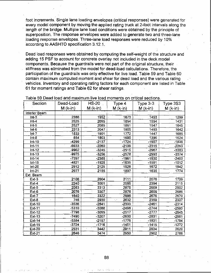
foot increments. Single lane loading envelopes (critical responses) were generated for every mode) component by moving the applied r~ting truck at 2-foot intervals along the length of the bridge. Multiple lane load conditions were obtained by the principle of superposition. The response envelopes were added to generate two and three-lane loading response envelopes. Three-lane load responses were reduced by 10.% according to AASHTO specification 3.12.1.

Dead load responses were obtained by computing the self-weight of the structure and adding 15 PSF to account for concrete overlay not included in the deck model components. Because the guardrails were not part of the original structure, their stiffness was eliminated from the model for dead-load calculations. Therefore, the participation of the guardrails was only effective for live load. Table 59 and Table 60 contain maximum computed moment and shear for dead load and the various rating vehicles. Inventory and operating rating factors for each component are listed in Table 61 for moment ratings and Table 62 for shear ratings.

Table 59 Dead load and maximum live load moments on critical sections. Section Dead-Load HS-20 Type4 Type 3-3 Type 383

M (k-in) M (k-in) M (k-in) M (k-in) M (k-in) Interior Beam

lnt-3 2386 1952 1673 1453 1299 lnt-4 2525 2095 1854 1554 1431 lnt-5 2527 2085 1861 1547 1645 lnt-6 2313 2047 1855 1493 1642 lnt-7 1833 , 1901 1772 1447 1685. lnt-8 854 1803 1695 1396 1624 lnt-10 -4299 -2137 -1724' -1907 ~1838

lnt-11 -6933 -2260 -2109 -2315 -2293 lnt-12 -9962 •3245 -2515 -2967 -3383 lnt-13 -9975 -3256 , -2578 -2993' -3374 lnt-14 -7397 -2388 -1961 -1930 -2400 lnt-15 -4821 -1928 -1635 -1591 -1512 lnt-20 2912 2·125 1928 1672 1842

· lnt-21 2977 2155 1897 1635 1774 Ext. Beam

Ext-3 2106 2604 2111 2076 1739 Ext-4 2240 3061 2586 2394 2115 Ext-5 2083 3313 2875 2609 2502 Ext-6 2076 3307 2876 26·09 2686 Ext:..7 1640 3322 2996 2676 2670 Ext-8. 746 2930 2632 2359 2337 Ext-10 -3536, -2841 -2303 -2461 -2314 Ext-11 -5310 -3088 -2498 -2744 -2593 Ext-12 -7798 -3095 -2517 -2777 -2645 Ext-13 -7490 -3207 -2600 -2831 , -2661 Ext-14 -5384 -2157 -1776 -1831 -1794 Ext-15 -3724 , -1716 -1451 -1415 -1272 Ext-20 2531 3442 r2911 2834 2620 Ext-21 2646 3474 2950 2902 2786

88

Table 60 Dead load and maximum live load shear on critical sections. Section EL# Dead-Load Hs.:.20 Type 4 Type 3-3 Type 3S3

V (kips) V (kips) V (kips) V (kips) V (kips) Interior Beam

lnt-1 43 -26.4 -25.6 -23.2 -20.9 -22.5 lnt-2 44 - -19.7 -21.3 -18.8 -16.5 -17.8 lnt-11 53 58.7 32.0 24.5 24.0 29.0 lnt-12 73 -69.2 -35.7 -30.0 -28.1 -29.2 lnt-13 72 70.4 36.3 28.5 28.9 31.7 lnt-14 56 -62.1 -33.3 -28.0 -27.5 -28.7

Ext. Beam Ext-1 - 1 -22.3 -23.2 -19.5 -18.5 -18.4 Ext-2 2 -17.0 -20.9 -18.2 -16.3 -16.3 Ext-11 32 -44.7 -25.7 -21.2 -20.8 -20.0 Ext-12 31 -50.5 -26.6 -22.0 -22.3 -21.4 Ext-13 13 -51.6 -31.1 -24.6 -28.0 -27.4 Ext-14 14 -46.2 -30.3 -'24.2 -26.9 . -26.4

T bl 61 L d R t" F t d t M a e oa a mQ ac ors ue o t Ell" t C k omen - 10 ree . Section HS-20 I Type4 Type 3-3 Type 3S3

Inv. Oper. Inv. Oper. Inv. Oper. Inv. Qper. Interior Beam

lnt-3 - 2.41 4.02 2.81 4.69 3.24 5.40 3.04 5.07 lnt-4 2.60 4.33 2.93 4.90 3.50 5.84 3.30 5.52 lnt-5 2.70 4.50 3.02 5.05 3.64 6.07 3.41 5.69 lnt-6 2.89 4.82 3.19 5.32 3.96 6.61 3.60 6.01 lnt-7 2.98 4.98 3.20 5.34 3.92 6.54 3.36 5.61 lnt-8 2.19 3.65 2.33 3.88 2.82 4.71 2.43 4.05 lnt-1 O 2.58 4.30 3.20 5.33 2.89 4.82 3.00 5.00 lnt-11 2.61 4.36 3.21 5.36 2.93 4.89. 2.96 4.93 lnt-12 2.32 3.87 3.00 5.01 2.48 4.14 2.19 3.65 lnt-13 2.35 3.92 2.96 4.95 2.49 4.16 . 2.20 3.68 lnt-14 2.83 4.72 . 3.44 5.74 3.47 5.79 2.81 4.69 lnt-15 2.89 4.83 3.41 5.70 3.51 5.86 3.69 6.16 lnt-20 2.65 4.42 2.92 4.87 3.36 5.61 3.05 5.09 lnt-21 2.58 4.31 2.93 4.89 3.39 5.67 3.10 5.17

Ext. Beam Ext-3 1.25 - 2.09 1.55 2.58 1.57 2.63 1.88 3.14 Ext-4 1.06 1.77 1.26 2.10 1.36 2.27 1.54 2.57 Ext-5 1.02 1.70 1.17 1.96 1.29 2.16 1.35 2.25 Ext-6 1.03 1.73 1.19 1.99 1.31 2.19 1.35 2.25 Ext-7 1.11 1.85 1.23 2.05 1.38 -2.30 1.38 2.30 Ext-8 1.08 1.80 1.20 . 2.00 1.34 2.24 1.35 2.26 Ext-10 .83 1.38 1.02 1.70 0.93 1.56 0.98 1.64 Ext-11 .97 1.63 1.20 2.00 1.10 1.83 1.16 1.94 Ext-12 .90 1.50 1.10 1.84 1.00 . 1.67. 1.05 1.75 Ext-13 .92 1.54. 1.13 1.89 1.03 1.71 1.08 1.80 Ext-14 1.42 2.37 1.72 2.87 1.67 2.79 1.63 2.73 Ext-15- 1.39 2.32 1.64 2.75 1.69 2.82 1.88 ' 3.13 Ext-20 .93 1.55 1.09 1.81 1.11 1.86 1.12 1.88 Ext-21 .91 1.51 1.06 1.77 1.08 1.81 1.12 1.88

...... -···

T bl 62 L d R t' F t d t Sh a e oa a mg ac ors ue o ear- Ell" t C k 10 ree . Section HS-20 · Type4 . Type 3-3 Type 3S3

Inv. Oper. Inv. Oper. Inv. Oper. Inv. Oper. Interior Beam

lnt-1 1.53 2.55 1.69 2.81 1.87 ·3.13 1.74 2.91 Int-2 2.05 3.42 2.32 3.88 2.65 4.43 2.45 4.09 Int-11 1.09 1.82 1.27 2.12 1.39 2.32 1.20 2.01 Int-12 1.13 1.89 1.35 2.25 1.44 2.40 1.26 2.11 lnt-13 1.17 1.96 1.35 2.26. 1.38 2.30 1.32 2.21 lnt-14 1.09 1.81 1.29 2.16' 1.32 2.20 1.25 2.09

Ext. Beam Ext-1 1.07 1.79 1.27· 2.12 1.34 2.23 1.35 2.25 Ext-2 1.33 2.22 1.53 2.55 1.71 2.85 1.70 2.84 Ext-11 1.20 2.01 1.46 2.43 1.49 2.48 1.54 2.57 Ext-12 1.30 2.17 1.57 2.62 1.55 2.59 1.61 2.69

. Ext-13 1.22 _2.04 1.54 2.57 1.35 2.26 1.38 2.31 Ext-14 1.01 1.68 1.26 2.11 1.13 1.89 1.16 1.93

Conclusions Recommendations

Load test results and model calibration procedures indicated that the RC guardrails provided a significant increase in the exterior beams stiffness. The effect of this is that more load is transferred to exterior beams. If contribution of the guardrails is included in the stiffness during load rating calculation it should also be included in the shear and moment capacity of the exterior beams. In the above ratings it was assumed to provide

. additional live-load capacity for positive moment and shear. In all cases the critical load ratings were controlled by negative moment of the exterior girders at a location approximately 9 feet from the piers. The condition of the guardrails should be thoroughly examined for cracking and attachment to the superstructure during future inspections.

If it is assumed that the RC guardrail cannot provide additional capacity, then the stiffening effects to the exterior girders should not be considered during load rating analyses. This condition was considered and the result was that the critical HS-20 Inventory rating factor was reduced to a factor of 0.6. The controlling factor was shear of the exterior girders near the piers. -


90

. ,:-· .....

Appendix A - Field Testing Procedures The motivation for developing a relatively easy-to-implement field testing system

was to allow short and medium span bridges to be tested on a routine basis. Original development of the hardware was started in 1988 at the Unive'rsity of Colorado under a contract with the Pennsylvania Department of Transportation (PennDOT). Subsequent to that project, the Integrated technique was refined on another study funded by the Federal Highway Administration (FHWA) in which 35 bridges located on the Interstate system throughout the country were tested and evaluated. Further r~finement has been implemented over the last several years.through testing and evaluating several more bridges, lock gates, and other structures. ·

The real key to being able to complete the field testing quickly is the use. of strain transducers (rather.than standard foil strain gages) that can be attached to the structural members in just a few minutes. These sensors were originally developed for monitoring dynamic strains on foundation piles during the driving process. They have been adapted for use in structural testing through special modifications, and have 3 to 4 percent accuracy, arid are periodically re-calibrated to NIST standards.

In addition to the strain sensors, the data acquisition hardware has been designed specifically for field use through the use of rugged cables and military-style connectors. This allows quick assembly of the system and keeps bookkeeping to a minimum. The analog-to-digital converter (ND) is an off-the-shelf-unit, but all signal conditioning, amplification, and balancing hardware has been specially designed for structural testing. The test software has been written to allow easy configuration (test length, etc.) and operation. The end result is a system that can be used by people other than computer experts qr electrical engineers·. Other enhancements include the use of an automatic remote-control position indicator. The Autoclicker, a device that electronically counts wheel revolutions, is mounted on the test vehicle over ·one of the wheels·. As the test vehicle crosses the structure along the preset path, a communication radio sends a signal to the strain measurement system that receives it and puts a mark in the data. This allows the field strains to be compared to anaiytical strains as a function of vehicle position, not only as a function of time.

The use of a moving load as opposed to placing the truck at discrete locations has two major benefits. First, the testing can be completed much quicker, meaning · there is less impact on traffic. Second, and more importantly, much more information can be obtained (both quantitative and qualitative). Discontinuities or unusual responses in the strain histories, which are often signs of distress, can be easily detected. Since the load position is monitored as well, it is easy to determine what loading conditions cause the observed effects. If readings are recorded only at discreet truck locations, the risk of losing information between the points. is great. The advantages of continuous readings have been proven over and over again.

The following list of procedures has been reproduced from the BDI Structural Testing System (STS) Operation Manual. This outline is intended to describe the general procedures used for completing a successful field test on a highway bridge using the 801-

91

'}·_- :··

STS. Other types of structures can be tested as well with only slight deviations from the directions given here.

· Once a tentative instrumentation plan has beeh developed for the structure in question, the strain transducers must be attached and the STS prepared for running the test.

Attaching Strain Transducers · There are two methods for attaching the strain transducers to the structural

members: C-claniping or with tabs and adhesive. For steel structures, quite.often the transducers can be clamped directly to the steel flanges of rolled sections or plate girders. If significant lateral bending is assumed to be present, then one transducer may be clamped to each edge of the flange. If the transducer is to be clamped, insure that the clamp is centered over the mounting holes. In general, the transducers can be clamped directly to painted surfaces. However, if the surface being clamped to is rough or has very thick paint, it should be deaned first with a grinder. The altemativEf to clamping is the tab attachment

. method outlined below.

1. Place two tabs in mounting jig. Place transducer over mounts and tighten the 1/4-20 nuts until they are snug (approximately 50 in-lb.). This procedure allows theJabs to mounted without putting stress on the transducer itself. When attaching transducers to RIC members, transducer extensions are used to obtain a longer gage length. In this case the extension is bolted to one end of the transducer and the tabs are bolted to the free ends of the transducer and the extension.

2. Mark the centerline of the transducer location ori the structure. Place marks 1-1/2 inches on either side of the centerline and using a hand grinder remove paint or scale

. from these. areas. If attaching to concrete, lightly grind the surface to remove any scale. If the paint is quite thick, use a chisel to remove most of it before grinding.

3. Very lightly grind the bottom of the transducer tabs to remove any oxidation or other contaminants.

4. Apply a thin line of adhesive to the bottom of each transducer tab.

5. Spray each tab and the contact area on the structural member with the adhesive accelerator.

6. Mount transducer in its proper location and apply a light force to the tabs (not the center of the transducer) for approximately 10 seconds.

If the above steps are followed, it should be possible to mount each transducer in approximately five minutes. When the test is complete, carefully loosen the 114:-20 nuts , from the tabs and remove transducer. If one is not careful, the tab will pop loose from the · structure and the transducer may be damaged. Use vice grips to remove the tabs from the structure.

92

.· .... ..

~ . ' . \

Assembly of System

Once the transducers have been mounted, they should be connected into an STS unit. The STS units should be placed near the transducer locations in such a manner to allow four transducers to be plugged in. Each STS unit can be easily clamped to the bridge girders. If the structure is concrete and no flanges are available to set the STS units on, transducer tabs glued to the structure and plastic zip-ties or small wire can be used to hold them up. Since the transducers will identify themselves to the system, there is no special order that they must follow. The only information that must be recorded is the transducer serial number and its location on the structure. Large cables are provided which can be . connected between the STS units. The maximum length between STS units is 50ft (1 Sm). If several gages are in close proximity to each other, then 'the STS units can be plugged directly to each other without the use of a eable. All connectors will "click'·' when the connection has been completed properly.

Once all of the STS units have been connected in series, one cable must be run and connected to the power supply located near the PC. Connect the 9-pin serial cable between the computer and the power supply. The position indicator is then assembled and the system connected to a power source (either 12VDC or 120-240AC). The system is now ready to acquire data.

Performing Load Test The general testing sequence is as follows:

1. Transducers are mounted and the system is connected together and turned on. . . . '

. . '

2. The deck is marked out for each truck pass. Locate the point on the deck directly above the first bearing for one of the fascia beams. If the bridge is skewed, the first point encountered from the direction of travel is used and an imaginary line extended across and normal to the roadway. All tests are started from this line. In order to track the position of the loading vehicle on the bridge during the test,· an X-Y coordinate system, with the origin at the selected reference point is laid out.

In addition to monitoring the longitudinal position; the vehicle's transverse position must be known. The transverse truck position is kept uniform by first aligning the truck in the center of the lane where it would normally travel at highway speed~ NeXt, a chalk mark is made on the deck locating the transverse location of the driver's side front wheel. By making a measurement from this mark to the reference point, the transverse (''Y'') position of the truck is always known. The truck is aligned on this mark for all

. subsequent tests in this lane. For two lane bridges with shoulders, tests are run on the shoulder (driver's side front wheel along the white line) and in the center of each lane. If the bridge has only two lanes and very little shoulder, tests are run in the center of each larie only. If the purpose of the test is to calibrate a computer model, it is sometimes more convenient to simply use the lane lines as guides since· it is easier for the driver to maintain a constant lateral position. Responses due to critical truck positions are then obtained by the analysis.

The driver is instructed that the test vehitle must be kept in the proper location on · the bridge. For example, the left front wheel needs to be kept ori the white line for the

93

·., ..

·. ;·

shoulder tests. Another important item is that the vehicles maintain a relatively constant rate of speed during the entire test. The process of converting data to a function of truck position assumes constant speed between each click mark.

Two more pieces of information are then needed: the axle weights and dimensions of the test vehicle. The driver generally.provides the axle weights, after stopping at a local scale. However, a weight enforcement team can use portable scales and weigh the truck at the bridge site. Wheel base and axle width dimensions are made with a tape measure and recorded.· ·

3. The program is started and the number of channels indidated is verified. If the number of channels indicated do not match the number of channels actually there, a malfunction has occurred and must be corrected before testing commences. ·

4. The transducers are initialized (zeroed out) with the Balance option. If a transducer cannot be initialized, it should be inspected·to ensure that it has not been damaged.

5 .. The desired test length, sample rate, and output file name are selected. In general, a longer test time than the actual event is selected. For most bridge tests, a one or twominute test length will suffice since the test can be stopped as soon as the truck crosses completely over the structure.

6. To facilitate presenting data as a function of load position, rather than time, two items describing the Pl information must be defined. The starting position and Pl interval distance allow the data to be plotted using position coordinates that are consistent with a numeric analysis. The starting position refers to the longitudinal position of the load vehicle in the model coordinate system when the data recording is started. The interval distance is the circumferenee of the tire that is being used by the Autoclicker. It is important that this information be clearly. defined in the field notes. ·

' 7. If desired, the Monitor option can be used to verify transducer output during a trial test. Also, it is useful to run a Position Indicator (Pl) test while in Monitor to ensure that the clicks are being received properly.

8. When all parties are ready to commence the test, the Run Test option is selected which places the system in an activated state. The Autoclicker is positioned so that the first click occurs at the starting line. This first click starts the test. The Autoclicker also puts one mark in the data for every wheel revolution. An effort should be made to get the truck across with no other traffic on the bridge. There should be no talking over the radios during the test, as a "position" will. be recorded each time the microphones are activated. · · · ·

e: When the test has been completed, and the system is still recording data, hit "S" to stop collecting data and finish writing the recorded data ·to disk .. If the data files are large,

· they can be compressed and copied to floppy disk.

1 O. It is important to record the field notes very carefully. Having.data without knowing where it was recorded can be worse.than having no data at all. Transducer location and

94

.. . . :·. .

serial numbers must be recorded accurately. All future data handling in BDl-GRF is then accomplished by keying on the transducer number. This system has been designed to eliminate the need to track channel numbers by keeping this process in the background. However, the STS unit and the transducer's connector number are recorded in the data file if needed for future hardware evaluations.

95

Appendix B - Modeling and Analysis: The Integrated Approach

Introduction

In order for load testing to be a practical means of evaluating short- to mediumspan bridges, i~ is apparent that testing procedures must be economic to implement in the field and the test results translatable into a load rating. A well-defined set of procedures must exist for the field applications as well as for the interpretation of results. An evaluation approach based on these requirements was first developed at the University of Colorado during a research project sponsored by the Pennsylvania Department of Transportation (PennDOT). Over several years, the techniques originating from this project have been refined and expanded into a complete bridge rating system. ..

The ultimate goal of the Integrated Approach is to obtain realistic rating values for highway bridges in a cost-effective manner. This is accomplished by measuring the response behavior of the bridge due to a known load and determining the structural parameters that produce the measured responses. ·With the availability of field measurements, many structural parameters in the analytical model can be evaluated that are otherwise conservatively estimated or ignored entirely. Items that can be quantified through this procedure include the effects of structural geometry, effective beam stiffnesses, realistic support conditions, effects of parapets and other non-structural components, lateral load transfer capabilities of the deck and transverse members, and the effects of damage or deterioration. Often, bridges ar~ rated poorly because of inaccurate representations ofthe structural geometry or because the material and/or cross-sectional properties of main structural elements are not well defined. A realistic rating can be obtained, however, when all of the relevant structural parameters are defined and implemented in the analysis process:

One of the most important phases of this approach is a qualitative evaluation of the raw field data. Much is learned during this step to aid in the rapid development of a representative model.

Initial Data Evaluation The first step in structural evaluation consists of a visual inspection of the data in the

form of graphic response histories. Graphic software was developed to display the raw strain data in various forms. Strain histories can be viewed in terms of time or truck position. Since strain transducers are typically placed in pairs, neutral axis measurements, curvature responses, and strain averages can also be viewed. Linearity between the responses and load magnitude can be observed by the continuity in the strain histories. Consistency in the · neutral axis measurements from beam to beam and as a function of load position provides great insight into the nature of the bridge condition. The direction and relative magnitudes of flexural responses along a beam line are useful in determining if end restraints play a significant role in the response behavior. In general, the initial data inspection provides the engineer with information concerning modeling requirements and can help locate damaged areas.

96

,:.·.·.,,·: .·

Having strain measurements at two depths on each beam cross-section, flexural curvature and the location of the neutral axis can be .computed directly from the field data. Figure 57 illustrates how curvature and neutral axis values are· computed from the strain measuremen'ts.

<J <J

LI

GB d -y -

GT~ [B

cD -[T - [B

-

d

Tronsciucers \______ [ B

Figure 57 Illustration of Neutral Axis and Curvature Calculations

The consistency in the N.A. values between beams indicates the degree of consistency in beam stiffnesses. Also, the consistency of the N.A. measurement on a single beam as a function of truck position provides a good quality check for that beam. If for some reason a beam's stiffness changes with respect to the applied moment (i.e. loss of composite action or loss of effective flange width due to a deteriorated deck), it will be observed by a shift in.the N.A. history.

Since strain values are translated from a function of time into a function of vehicle position dn the structure and the data acquisition channel and the truck position tracked, a considerable amount of book keeping is required to perform the strain comparisons. In the past, this required manipulation of result files and spreadsheets which was tedious and a major source of error. This process in now. performed automatically by the software and all of the information can be verified visually.

Finite Element Modeling and Analysis The primary function of the load test data is to aid in the development of an accurate

finite element model of the bridge. Finite element analysis is used because it provides the most general.tool for evaluating various types of.structures. Since a comparison of measured and computed responses is performed, it is necessary that the analy~is be able to represent the actual response behavior. This requires that actual geometry and boundary conditions be realistically represented. In maintaining reasonable modeling efforts and computer run times, a certain amount of simplicity. is also required, so a planar grid model is generated.for most structures and linear-elastic responses are assumed. A grid of frame elements is assembled in th~ same geometry as the actual structure. Frame

97

·':.',, .•· ' •' ,·

"elements represent the- longitudinal and transverse members of the bridge. Plate elements attached to the grid provide the load transfer characteristics of the deck. When endrestraints are determined to be present, elastic spring elements having both translational and rotational stiffness te!""1s are inserted at the support locations.

The connection between the beams and the deck plates can be handled in various ways. The simplest, and generally the most accurate, method is to assume all of the beam neutral axes lie in a single plane. Any contribution of the deck resulting in composite action is then accounted for by the beam moment-Of-inertia values. This met.hod is most suitable when the primary beam load response is flexure.

An alternate approach, providing a more realistic model of the beam/deck inter~ction, is the use of eccentricity terms in the beam elements. This is a quasi 3-D modeling technique that separates the plane of the beam neutral axes with the plane of the deck. It is useful when modeling composite beam/slab structures with a variety of different beam cross-se.ctions such that a single plane cannot be assumed. While the geometry of this model is technically more realistic, a much finer mesh is required because flexural responses are partially resisted by first-ord.er axial terms of the beam elements. The resulting moment and axial force responses are much more discretized than.with the pure planar model. Another draw back to the quasi 3-D model becomes apparent during data processing .of the analysis results because beam stresses are a function-of beam flexure and axial deformation.

Depending on the structure's geometry, a planar model may not be sufficient. For example trusses, box girders, and structures containing beams with depth-to-span ratios greater than 10 generally required 3-D modeling techniques to accurately represent load transfer characteristics. The method of modeling is therefore dependent on the complexity of the struct~re, the type of information that is sought, and the preference of the engineer.

Loads are applied in a manner similar to the actual load test. A model of the test truck, defined by a two-dimensional group of point loads, is placed on the structure model at discrete locations along the same path that the test truck followed during the load test. Gage locations identical to those in the field are also defined on the structure model so that strains can be computed at the same locations under the same loading conditions.

Model Correlation and Parameter Modifications The accuracy of the model is determined numerically by the analysis using several

statistical relationships and through visual comparison of the strain histories. The numeric accuracy values are usefl,JI in evaluating the effect of any changes to the model, where as the graphieal representations provide the engineer with the best perception for why the model is responding differently than the measurements indicate. Member properties that cannot be accurately defined by conventional methods or directly from the field data are evaluated by comparing the computed strains with the measured ·strains. These properties are defined as variable and are evaluated such that the best correlation between the two sets of data is obtained. It is the engineer's responsibility to determine which parameters need to be refined and to assign realistic upper and lower limits to each parameter. The evaluation of the member property is accomplished with the aid of a parameter identification process (optimizer) built into the analysis. In short, the process consists of an

98

...... ··.· ,,

'' '/,

iterative procedure of analysis, data comparison, and parameter modification. It is important to note that the optimization process is merely a tool to help evaluate various modeling parameters. The process works best when the number of parameters is minimized and

, reasonable initial values are used.· ·

During the optimization process, various error values are computed by the.analysis program that provide quantitative measure of the model accuracy and improvement. The error is quantified in four different ·ways, each providing a different perspective of the model's ability to represent the actual structure; an absolute error, a percent error, a scale error and a correlation coefficient.

The absolute error is computed from the absolute sum of the strain differences . . Algebraic differences between the measured and theoretital strains are computed at each gage location for each truck position used in the analysis, therefore, several hundred strain comparisons are ,generally used in this calculation. This quantity is typically used to determine the relative accuracy from one model to the next and to evaluate the effect of various structural parameters. It is used by the optimization algorithm as the objective

· function to minimize. Because the absolute error is in terms of micro-strain (me) the value can vary significantly depending on the magnitude of the strains, the number of gages and number of different loading scenarios. For this reason, it has little conceptual value except for determining the relative improvement of a particular model.

A percent error is calculated to provide a better qualitative measure of accuracy. It is computed as the sum of the strain differences squared divided by the sum of the · measured strains squared. The terms are squared so that error values of different sign will not cancel each other out, and to put more emphasis on the areas with higher strain magnitudes. A model with acceptable accuracy will usually have a percent error of less than 10%.

The scale error is similar to the percent error except that it is based on the maximum error from each gage divided by the maximum strain value from each gage. This number is useful because it is based only on strain measurements recorded when the loading vehicle is in the vicinity of each gage. Depending on the geometry of the structure, , . '

the number of truck positions, and various other factors, many of the strain readings are essentially negligible. This error function uses only the most relevant measurement from each gage.

Another useful quantity is the correlation coefficient which is a measure of the linearity between the measured and computed data. This value determines how well the shape of the computed response histories match the measured responses. The correlation coefficient can have a value between 1.0 (indicating a perfect linear relationship) and -1.0 (exact opposite linear relationship). A good n:iodel will generally have a correlation .

' '

coefficient greater than 0.90. A poor correlation coefficient is usually an indication that a major error in the modeling process has occurred. This is generally caused by poor representations of the boundary conditions or the loads were applied incorrectly (i.e. truck. traveling in wrong direction).

99

.,,. ____________ _

The following table contains the equations used to compute each of the statistical, error values:

Table 63. Error Functions

ERROR FUNCTION EQUATION

Absolute Error I:lsm - sci

Percent Error ' 2 2 . I:(sm - sc) I I:( &m)

Scale Error I:maxlsm - sclgage

L maxi &ml gage

Correlation Coefficient - -

L.(&m - sm)( &c - sc)

L 'rsm - &m) (&c - &c) ~ -2 -2

In addition to the numerical comparisons made by the program, periodic visual comparisons of the response histories are made to obtain a conceptual measure of accuracy. Again, engineering judgment is essential in determining which parameters should be adjusted so as to obtain the most accurate model. The selection of adjustable parameters is 'performed by determining what properties have a significant effect on the strain comparison and determining which values eannot be accurately estimated through conventional engineering procedures. Experience in examining the data comparisons is helpful, however, two general rules apply concerning model refinement. When the shapes of the computed response histories are similar to the measured strain records but the magnitudes are incorrect this implies that member stiffnesses must be adjusted. When the shapes of the computed and measu~ed response histories are not very similar then the boundary conditions or the structural geometry are not well represented and must be refined. ·

In some cases, an accurate model cannot be obtained, particularly when the responses are observed to be non-linear with load position. Even then, a great deal can be learned about the structure and intelligent evaluation decisions can be made.

100

.~... .··· .

Appendix C - Load Rating Procedures

For borderline bridges (those that calculations indicate a posting is required), the primary drawback to conventional bridge rating is an oversimplified procedure for estimating the load applied to a given beam (i.e. wheel load distribution factors) and a poor representation of the beam itself. Due to lack of information and the need for conservatism, material and cross-section properties are generally over-estimated and beam end supports are assumed to be simple when in fact even relatively simple beam bearings have a substantial effect on the midspan moments. Inaccuracies associated with conservative assumptions are compounded with complex framing geometries. From an analysis standpoint, the goal here is to generate a model of the structure that is capable of reproducing the measured strains. Decisions concerning load rating are then based on the performance of the model once it is proven to be accurate.

The main purpose for obtaining an accurate model is to evaluate how the bridge will respond when standard design loads, rating vehicles or permit loads are applied to the structure. Since load testing is generally not performed with all of the vehicles of interest, an analysis must be performed to determine load-rating factors for each truck type. Load rating is accomplished by applying the desired rating loads to the model and computing the stresses on the primary members. Rating factors are computed using the equation specified in the AASHTO Manual for Condition Evaluation of Bridges - see Equation (1 ).

it is important to understand 'that diagnostic load testing and the integrated approach are most applicable to obtaining Inventory (service load) rating values. This is because it is assumed that all of the measured and computed responses are linear with respect to load.

· The integrated approach is an excellent method for estimating service load stress ·values but it generally provides little additional information regarding the ultimate strength of particular structural members. Therefore, operating rating values must be computed using conventional assumptions regarding member capacity. This limitation of the integrated approach is not viewed as a serious concern, however, because load responses should never 'be permitted to reach the inelastic range.

Operating and/or Load Factor rating values must also be computed to ensure a factor of safety between the ultimate strength and the maximum allowed service loads. The safety to the public is of vital importance but as long as load limits are imposed such that the structure is not damaged then safety is no longer an issue.

Following is an· outline describing how field data is used to help in developing a load rating for the superstructure. These procedures will only complement the rating process, and must be used with due consideration to the substructure and inspection reports.

1. Preliminary Investigation: Verification of linear and elastic behavior through continuity of strain histories, locate neutral axis of flexural members, detect moment resistance at beam supports, qualitatively evaluate behavior.

2. Develop representative model: Use graphic pre-processors to represent the actual geometry of the structure, including span lengths, girder spacing, skew, transverse

101

members, and deck.· Identify gage locations on model identical to those applied in the field.

3. Simulate load test on computer model: Generate 2-c:limensional model of test vehicle and apply to structure model at discrete positions along same paths defined during, field tests. Perform analysis and compute strains at gage location for each truck position.

4. Compare measured and initial computed strain values: Various global and local error values at each gage location are computed and visual comparisons made with · post-processor.

5. Evaluate modeling parameters: Improve model based on data comparisons. · Engineering judgment and experience is required to determine which variables are to

be modified. A combination of direct evaluation techniques and parameter optimization are used to obtain a realistic model. General rules have been defined to simplify this operation. ·

6. Model evaluation: In some cases it is not desirable to rely on secondary stiffening effects if it is likely they will not be effective at higher load levels. It is beneficial; though, to quantify their effects on the structural response so that a representative computer model can be obtained. The stiffening effects that are deemed unreliable can be eliminated from the model prior to the computation of rating factors. For instance, if a non-composite bridge is exhibiting composite behavior, then it can conservatively be ignored for rating purposes. However, if it has been in service for 50 years and it is still behaving compositely, chances are that very heavy loads have crossed over it and any bond-breaking would have already occurred. Therefore, probably some level of composite behavior can be relied upon. When unintended composite action is allowed in the rating, additional load limits should be computed based on an allowable shear stress between the steel and concrete and an ultimate load of the non-composite structure.

7. Perform load rating: Apply H.S-20 and/or other standard design, rating and permit loads to the calibrated model. Rating and posting load configuration recommended by AASHTO ~re shown in Figure 58.The. same rating equation specified by the AASHTO -Manual for the Condition Evaluation of Bridges is applied:

where: RF= C= D= L=

A1= A2= I=

. RF= C - AJD A2L(J + I)

Rating Factor for individual member. Member Capacity. Dead-Load effect. -Live-Load effect. Factor applied to dead-load. Factor applied to live-load. Impact effect, either AASHTO or measured.

102

(1)

The only difference between this rating technique and standard beam rating programs is that a more realistic model is used to determine the dead-load and live-load effects. Two-dimensional loading techniques are applied because wheel load distribution factors are not applicable to a planar model. Stress envelopes are · generated for several truck paths, envelopes for paths separated by normal lane widths are combined to determine multiple lane loading effects.

8. Consider other factors: Other factors such as the condition of the deck and/or substructure, traffic volume, and other information in the inspection report should be taken into consideration and the rating factors adjusted accordingly.

Axle Loads 8 32 32 (kips)

j· f ·j 14.0' 14.0' to 30.0'

Axle No. 1 2 3 HS-20 VEHICLE WEIGHT = 72 KIPS (36 TONS)

A•"(~;~~~' '[- '5.0 -l-< o ~r

Axle No. 1 2 3

TYPE 3 VEHICLE WEIGHT = 50 KIPS (25 TONS)·

Axle Loads 1 0 (,;,,, l· 11.0' . 22.0'

Axle No. 1 2 3 TYPE 3S2 VEHICLE WEIGHT = 72 KIPS (36 ·TONS)

A•r~·j~~-.~~-1_5._o·~~-.-:+[-4_.o_·:+f-·-.~~1_5_.o·~~~·*I-·-.~~-,_6._o·~~~~J~·-4._o·~J Axle No. 1 2 3 4 5 6

TYPE 3-3 VEHICLE WEIGHT = 80 KIPS (40 TONS)

Figure 58 AASHTO rating and posting load configurations.

103

Appendix D - References

AASHTO (1989). "Standard Specification for Highway Bridges." Washington,D.C.

AASHTO, (1994). "Manual for the Condition Evaluation of Bridges", Washington,D.C.

Commander,B., (1989). "An Improved Method of Bridge Evaluation: Comparison of Field Test Results with Computer Analysis." Master Thesis, University of Colorado, Boulder, CO. ·

Gerstle, K.H., and. Ackroyd,M.H. (1990). "Behavior and Design of Flexibly-Connected·. Building Frames." Engineering Journal, AISC, 27(1),22-29.

Goble,G., Schulz,J., and Commander,B. (1992). "Load Prediction and Structural Response." Final Report, FHWA DTFH61-88-C-00053, University of Colorado, Boulder, CO.

Lichtenstein,A.G.(1995). "Bridge Rating Through Nondestructive Load Testing." Technical Report, NCHRP Project 12-28(13)A.

Schulz,J.L. (1989). "Development of a Digital Strain Measurement System for Highway Bridge Testing." Masters Thesis, University of Colorado, Boulder, CO.

Schulz,J.L. (1993). "In Search of Better Load Ratings." Civil Engineering, ASCE 63(9),62-65 ..

104

load testing and load rating eight state highway bridges...

Documents