loan repayment behaviour of farmers: analysing...

Loan Repayment Behaviour of Farmers: Analysing

Indian Households

Tanika Chakraborty1

Aarti Gupta2

1Indian Institute of Technology, Kanpur. Email:[email protected] Institute of Technology. Email:[email protected]

Abstract

This paper uses the IHDS 2009-10 to analyse the nature and extent of indebtedness

of Indian households. It studies utilisation of loans taken from formal versus informal

sector and the subsequent loan repayment behaviour of these households.By analysing

repayment patterns we identify the characteristics of individuals who are defaulting.

We study the source and purpose of borrowing, consumption and production patterns

of households taking loan from different sources to gain insight towards the existence

of moral hazard problem. We find that people who borrow from formal sources

tend to have higher consumption, higher social spending and lower investment as

opposed to people who borrow from informal sources. Higher spending, as opposed

to investment, in turn has a negative impact on loan repayment. Our findings point

towards the differential treatment of formal versus informal loans by the households.

We argue that people tend to under-utilise default more on loans that are taken from

sources which impose lesser punishment in the future.

Borrowing & Lending Behaviour of Households

Introduction

Debt plays an essential role in the lives of the rural households in developing countries

in a number of ways. It is an important instrument for smoothing consumption, in a

context where incomes typically experience large seasonal fluctuations. [Ghosh et al.,

2000] However, credit markets in developing nations especially in rural households

do not behave completely like competitive markets. They are dual structured, where

formal and informal financial systems operate side by side. Due to the lack of

availability of a properly structured debt market in the rural areas of the country,

majority of the households borrow from informal sources of finance which charge high

interest rates and often lead to informal agents usurping the assets of the households.

To provide easier access to credit we often find governments intervening in the

workings of the credit market in multiple ways. In Thailand increased participation

in formal financial institutions increased economic growth between 1976 and 1990

[Townsend and Ueda, 2003].

India was also no different. Under the 1949 Banking Regulation Act, all banks

required to obtain a banking licence from the Reserve Bank of India, which is the

Indian Central Bank prior to opening of a new branch. In 1975, the Narsimham

committee conceptualised the creation of Regional Rural Banks (RRB). According

to the RRB act of 1976, their equity is partly held by the Central Bank, partly

by the state bank and the remaining by the sponsoring bank. The main aim was

to develop the rural economy by providing credit to small and marginal farmers,

agricultural labourers, artisans and small entrepreneurs [Misra et al., 2006]. In 1977,

the government of India wanted to increase access of credit in the rural areas of

the country. As a means of ensuring this, they mandated that a bank can obtain a

license to open a branch in an already banked location only if it opened branches

in four unbanked locations [Burgess and Pande, 2004]. Rural lending rates were

also kept much below the urban lending rates. Every branch was also required to

maintain a credit-deposit ratio of 60 percent within its geographical area of operation

[Burgess et al., 2005]. However, given the size of the Indian credit market these

interventions were perhaps not significant enough to satisfy the credit needs of poor

households. Although progress has been made, formal finance does not appear to

Aarti Gupta Chapter 0 1


have adequately permeated vast segments of our society [Hoda and Terway, 2015].

Indian households primarily borrow from two sources, the formal and informal sources.

The formal sector constitutes of all institutional credit agencies like co-operative banks,

commercial banks, government lending agencies, regional rural banks, insurance

etc. On the other hand the informal sector comprises of the non institutional

credit agencies like landlords, agricultural moneylenders, professional money lenders,

traders and commission agents, relatives and friends. Prior to the First Plan in

1951, all the financial requirements for the rural sector for agricultural purposes

were met by traditional/informal sources of finance, primarily the moneylender.

The share of provision of credit by commercial banks or cooperative societies was

barely 4% by June 1951 [Pradhan, 2013]. With the government pushing its credit

agencies to expand its credit facilities with special emphasis on providing it to

the rural agricultural sector, the access and availability of formal credit has vastly

increased. However, one cannot deny that both formal and informal sector still

form an important aspect of the lending scenario in Indian agricultural households.

Banerjee and Duflo [2007] show that a vast majority of people in Hyderabad that

have a per capita income of below two dollars borrow from non institutional sources

even though they have access to formal loans. Madestam [2014] developed a model

in which they model how informal finance complements the banks by permitting for

larger formal loans to poor borrowers. They suggest that formal banks have access

to unlimited funds but lack proper monitoring of loans. Informal lenders can prevent

non-diligent behaviour but often lack the needed capital.

Formal and informal sector differ vastly in their lending methodologies. The size of

loans offered, the interest rates charged, the tenure of the loans, repayment schedules

etc are different when a household borrows from a formal source as opposed to

an informal source. Repayment of loans depends on the terms of the loan and

the utilisation of the loan [Bhattacharjee, 2014]. Researchers studying household

sectoral choice between formal and informal finance find that in spite of availability

of formal loan, informal rural credits are still vastly popular. Part of the reason is

the easy and adequate access to informal sources [Pal, 2002]. Prompt recovery of

informal credit where creditors employ informal recovery techniques like reputation

mechanism or third party enforcement also make it more viable. In fact, this has



been the underlying principle driving the growth of microcredit in India.

We know that formal and informal loans have different terms of the loan. Hence

it is possible that the borrowing source affects the expectation of households about

the associated penalty. This in turn is likely to affect the way households decide to

utilise loans from different sources. To get a further insight into this and explore why

this happens we need to understand how farmers utilise loans taken for agricultural

purposes from formal sources. One of the main arguments for the pushing of

governments to set up rural banks was to provide easier credit access to agricultural

households and combat the high interest rates charged by moneylenders. But over

the years several questions have been raised at the efficacy of political interventions

in the credit systems.

On the one hand lower interest rates on formal sources should drive productivity.

However easier availability could also increase unproductive spending which could

lead towards non repayment. In order to understand this better this paper analyses

the borrowing behaviour of households. It studies both investment and consumption

patterns of households to analyse their relationship with loan repayment. This paper

tries to study whether the source of loans has any bearing on the behaviour and

decision making of the households. Specifically we ask whether borrowing from

formal lending agencies as opposed to informal lending agencies alter household′s

consumption and investment decision. We study if these decisions are altered how

they affect the repayment capacity of these households. The next section looks at

the data used to analyse these questions.

There are many studies that analyse non-repayment of loans taken by households

(Field and Pande [2008], Rajeev and Mahesh [2010], Gine et al. [2013]). Inability

to repay a loan can be due to a shock faced by the household. For instance, the

household could default due to adverse shocks like natural calamities, earnings or

employment shocks or health shocks. However, non-repayment could also arise due

to moral hazard problems associated with easier access to loans.

Although the theoretical literature on repayment decisions of households is recent,

the question has fairly been in the macro literature for quite some time. In the

macroeconomics literature, the decision to default is often modelled as a function of



the cost of default, including legal costs. Further, agents need to weigh the benefits

of default against the consequences of autarky. Jeffrey Sachs first introduced the

concept of debt relief for countries [Sachs, 1989]. Paul Krugman formalised the actual

derivation of the debt relief curve and the underlying logic behind it [Krugman, 1988].

Krugman′s paper examines the tradeoffs facing creditors of a country whose debt is

large enough that the country cannot attract voluntary new lending. According to

Krugman if a creditor country was trying to affect the adjustment efforts of a debtor

country, the more debt relief it would give, larger would be the adjustment effort by

the debtor country to service the debt. If the debt were too large then the debtor

country would have no incentive to put in any effort to pay off the debt.

Background

Exclusion from the banking sector has huge welfare costs, especially for the poor. One

of the major problems with informal sector lending is the high interest rate and the

usurping of assets from the rural household in the event of a default. Informal finance

is often thought to be anti-developmental, exploitative, and prone to consumption

rather than investment behavior [Von Pischke et al., 1983] This has led to frequent

interventions by the government in the banking sector of many low income countries.

For instance, Mexico nationalized its banks in 1982, Nigeria and Philippines made it

compulsory for its banks to lend a certain percentage to priority sectors [Besley, 1995].

This ensures that credit facilities are available to the poorer sections of the country at

a cheaper rate. India has also experienced large banking programs under the flagship

of the government at various times. Traditionally, majority of the population in the

country borrowed from informal sources like money lenders, friends and relatives.

With a view to reducing poverty, dependence on informal loans and increasing access

to credit in the rural areas, the government set up 30000 bank branches between

1969-1990 in rural locations. Priority was given to locations with no prior formal

credit and savings institution [Burgess and Pande, 2004]. The Indian central bank in

1977,committed to increasing bank presence in rural areas by adopting a 1:4 policy,

which was establishing 4 rural branches for every urban branch. In addition to this in

1980 the central bank adopted its directed lending policy which required all banks to



lend at least 40% of the loaned amount to priority sectors, like agriculture [Burgess

and Pande, 2004]. The central bank aimed to achieve this target by 1985.

These policies have resulted in increase of the overall loans issued for agriculture

and allied activities from all the institutional sources from 13.89 billion in 1980-81 to

1071.62 billion in 2011-12. The overall loan amount outstanding also increased at a

similar pace from 42.89 billion in 1980-81 to 2195 billion in 2011-12 [RBI, 2014].There

is evidence that increase in formal banking institutions has reduced poverty and

increased access to credit of farmers. Despite these improvements the reach of the

formal banking sector falls short of smoothing weather shocks and price uncertainties.

This is often cited as a reason behind increase in suicide rates amongst the farming

community in India Mishra [2006]. On average, the decade from 1996-2006 has seen

about 16,000 farmers commit suicide every year.[Nagaraj, 2008]. To combat this

dramatic socio economic rural problem a number of state level and nationalised loan

waiver schemes have been announced in the last two decades. In 2008, Debt-Relief

scheme for small and marginal farmers, announced by the central government waived

Rs 650 billion of debt held by farmers issued by commercial and cooperative banks

between the years 1997-2007. In 2012, Uttar Pradesh Chief Minister announced a

Rs 16.50 billion worth of debt relief for farmers in UP (Jagran Josh, 2012).As recent

as 2014, the Telengana and Andhra Pradesh governments announced massive loan

waiver schemes. Jumping on the loan waiver band wagon the winning party in Tamil

Nadu 2016 state elections waived Rs 57.80 billion of crop loans [?]. While loan waivers

are often the preferred instrument of governments to alleviate rural poverty and

insure weather shocks, seldom choice is made on the basis of research findings about

their efficacy on targeting the poor farmers. If, for instance households are indeed

more likely to default on formal loans as opposed to informal, then loan waivers

would only encourage households to use formal loans for unproductive purposes in

the expectation of a future waiver.

With agricultural credit expanding at an increasing rate in the last couple of decades

(Reserve Bank of India, 2014) and Indian government continuing to push formal

sources of borrowing, it has now become increasingly important to understand the

efficacy of this line of policy interventions and see how borrowers respond to the

loans taken from formal sources as opposed to informal sources. Existing research



provides some evidence that loan waivers alter the borrowing behaviour of farmers.

Kanz [2012] suggests in his paper analysing the 2008 national debt waiver scheme,

that such economic stimulus programs may distort borrower incentives and give rise

to moral hazard. To get a further insight into this and explore why this happens we

need to understand how farmers utilise loans taken from various sources.

Typically there are a number of sources from where an Indian household can borrow.

But loan waivers from government are primarily given to loans taken for agricultural

purposes from formal sources, particularly nationalised rural banks. One of the

main arguments in favour of expanding access to formal credit at low rates of return

was to protect poor farmers from steep informal interest rates.Lower interest rates

on formal sources should drive productivity. However easier availability could also

increase unproductive spending which could lead towards non repayment. This paper

analyses the borrowing behaviour of households. It studies how investment and

consumption patterns of households varies with the source of loan and analyse their

relationship with loan repayment.

Data & Descriptive Statistics

We use loan repayment and consumption data from the 2005 India Human De-

velopment Survey (IHDS), a nationally representative data of 41554 households,

collected by the National Council of Applied Economic Research in New Delhi and

the University of Maryland. Out of the 41,554 households our paper focuses on

only those households which have taken a loan, thus reducing the sample size to

16,900 households. To understand loan repayment behaviour, it is important to look

into the purpose of borrowing, source of borrowing, interest rates and consumption

details. The IHDS is a unique survey, providing detailed information on consumption,

investments, social spending and borrowing behaviour of these households.

Despite the aggressive efforts by the government to increase access to loan from

formal sources, through the social banking program and various other policies the

IHDS data shows that close to 70% of the households still borrow from informal



sources like moneylenders, relatives and friends. Table 1 provides a summary of the

borrowing behaviour of households in urban and rural regions. 32.75% of households

borrow from formal sources like banks, NGOs and employers, while 67.25% borrow

from informal sources like moneylenders, relatives and friends. Almost half, 47.3% of

the formal loans are agricultural or business loans, in contrast to 16.67% of informal

loans. However, when we restrict the sample to just rural households the percentage

of households who borrow from informal sources for the purpose of agriculture is

higher.



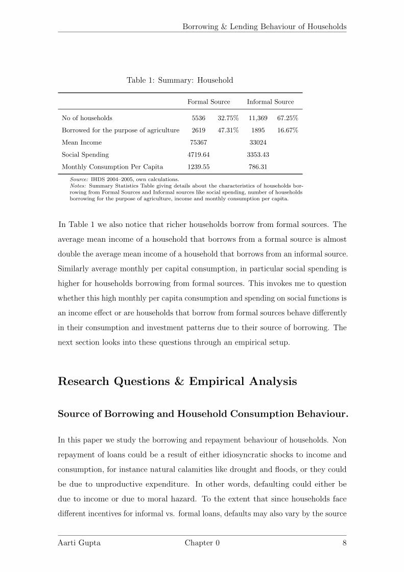
Table 1: Summary: Household

Formal Source Informal Source

No of households 5536 32.75% 11,369 67.25%

Borrowed for the purpose of agriculture 2619 47.31% 1895 16.67%

Mean Income 75367 33024

Social Spending 4719.64 3353.43

Monthly Consumption Per Capita 1239.55 786.31

Source: IHDS 2004–2005, own calculations.Notes: Summary Statistics Table giving details about the characteristics of households bor-rowing from Formal Sources and Informal sources like social spending, number of householdsborrowing for the purpose of agriculture, income and monthly consumption per capita.

In Table 1 we also notice that richer households borrow from formal sources. The

average mean income of a household that borrows from a formal source is almost

double the average mean income of a household that borrows from an informal source.

Similarly average monthly per capital consumption, in particular social spending is

higher for households borrowing from formal sources. This invokes me to question

whether this high monthly per capita consumption and spending on social functions is

an income effect or are households that borrow from formal sources behave differently

in their consumption and investment patterns due to their source of borrowing. The

next section looks into these questions through an empirical setup.

Research Questions & Empirical Analysis

Source of Borrowing and Household Consumption Behaviour.

In this paper we study the borrowing and repayment behaviour of households. Non

repayment of loans could be a result of either idiosyncratic shocks to income and

consumption, for instance natural calamities like drought and floods, or they could

be due to unproductive expenditure. In other words, defaulting could either be

due to income or due to moral hazard. To the extent that since households face

different incentives for informal vs. formal loans, defaults may also vary by the source



of loans. Theoretically, there have been various arguments that households might

behave differently when borrowing from a formal source like banks as opposed to an

informal source like money lenders. For instance, if monitoring is stricter for loans

taken from relatives and moneylenders then the defaults would be lower on informal

loans [Banerjee and Duflo, 2007].

On the other hand in the absence of stricter monitoring, households misuse agricul-

tural loans borrowed from formal institutions, leading to default. Table 2 summarises

the behavioural patterns of people who have repaid their loan as opposed to those

who have not. Analysing the incidence of non-repayment we see that 73% of the

households who have borrowed a loan have not repaid their loan. Dissecting these

households we notice that majority of them belong to the rural areas as opposed to

urban. Amongst the 12,284 households who have not repaid their loans, households

who have borrow for the purpose of agriculture constitute the largest group (29.66%)

as opposed to marriage (16.15%) or buying a house (15.89%). This indicates that

people who borrow for the purpose of agriculture are most likely to default on their

loans. Does this mean that people who borrow for agricultural purposes indulge in

unproductive expenditure or are there any other underlying socioeconomic charac-

teristics within these households which contribute towards the non-repayment? To

investigate these possibilities we first empirically explore whether borrowing from

formal sources as opposed to informal sources has an impact on investment and

consumption patterns of a household.



Table 2: Analysing Repayment Rates of Households by Purpose of Borrowing

Frequency Non Repayment

RURAL URBAN

Total Households 16934 12284 71% 29%

HH borrowed for the purpose of agriculture 5196 3635 83% 17%

HH borrowed for the purpose of marriage 2604 1980 71% 29%

HH borrowed for the purpose of buying a house 2758 1948 59% 41%

HH borrowed for the purpose of consumption 2078 1569 67% 33%

HH borrowed for medical purposes 2393 1833 70% 30%

HH borrowed for the purpose of education 409 306 44% 56%

HH borrowed for the purpose of buying land 171 121 65% 35%

Source: IHDS 2004–2005, own calculations.Notes:Repayment Rates: Table giving details about repayment rate of households and segregating themaccording to the purpose of borrowing.

We start by investigating whether two households with the same amount of outstand-

ing loan and with the same overall income differ in their consumption behaviour

depending on the source from which they borrowed. To do this we estimate the

following model in a liner probability framework.

COPCiv = α1 + α2LF i + α3logI iv +k∑

i=4

αiXiv + Eiv (1)

where COPC is monthly consumption per capita of household i in village v. In IHDS

data this reflects the primary sampling unit, roughly the size of an average Indian

village. The IHDS survey asked a series of 47 questions about household consumption

designed to estimate total household consumption expenditures. COPC is calculated

as a sum total of the expenditures on these 47 consumption items. LF is an indicator

reflecting whether household i took a loan from a formal source. LogI is log of total

household income. Xi is an additional set of covariates such as household size, caste

and religion. Ei represents PSU level fixed effects capturing idiosyncratic shocks

that are specific to a village. For instance it captures village specific weather shocks

that might affect consumption in a village and also affect availability of formal loans



if more drought prone villages are better covered by government banks. Our primary

parameter of interest is α2 which captures any difference in consumption behaviour

of households caused by the difference in their source of borrowing.

In our next section we analyse the relationship between a household′s level of social

spending, which is the amount of money a household spends on social functions like

festivals, birth, death etc and its source of borrowing.

Source of Borrowing and Household Social Spending.

Utilisation of loans borrowed for agricultural purposes have interested researchers for

a long time. Tiwari [2012] suggests that 40% of the loan amount borrowed by farmers

for agricultural purposes is used on non agricultural purposes such as marriages,

education, and health etc. Similarly Banerjee and Duflo document how people spend

a considerable portion of their income on festivals and other social functions despite

scraping through for bare necessities like food, clothing and housing. They find that

in Udaipur the extremely poor spend 14% of their budget on festival [Banerjee and

Duflo, 2007].

Khamis et al. [2012] also find evidence supporting the consumption of visible goods

by socially disadvantaged groups. They suggest that these consumption patterns can

be partly explained as a result of the status signalling nature of the consumption

items. To the extent that formal loans are less monitored, households are more likely

to undertake unproductive expenditures from these formal loans. Accordingly we

investigate the effect of borrowing from a formal source on social spending and the

effect of social spending on loan repayment. Social spending in the IHDS, records the

amount of money spent by a household on social functions like marriages, festivals,

birth death etc. Table 3 shows that the average social spending of all the households

in our dataset is Rs 2922. Households who have not repaid their loan have a mean

social spending of Rs 4221 as opposed to the mean social spending of Rs 3045 for

households who have repaid their loan. One could argue that income could be a

determining factor in deciding how much a household spends on social functions.

But we notice that the average income of households who have repaid their loan is



higher, while their social spending is lower compared to the households who have

not repaid their loan.

Table 3: Descriptive Statistics

Income COPC Social Spending Investment Ratio

Obs Mean Obs Mean Obs Mean Obs Mean

Full Sample 41553 84293.06 41554 953.64 41490 2922.18 14096 0.097

HH who took a loan 16909 72939.01 16909 934.64 16905 3902.50 7122 0.108

HH who have repaid their loan 4650 79936 4650 995.08 4650 3045.73 2038 0.124

HH who have defaulted 12284 70313.66 12284 911.42 12280 4220.92 5094 0.102

HH borrowed from formal sources 5536 109801.6 5536 1239.55 5534 4719.64 2562 0.152

Source: IHDS 2004–2005.Notes: The above table gives us the detailed descriptive statistics of the variables primarily used from the IHDS data, givingdetails about the characteristics of households like their Income, COPC, Social Spending and Investment Ratio. Income refers tothe annual income of a household. COPC is Monthly Consumption Per Capita. Social Spending refers to the amount of moneya household spends in a year on social functions like marriage etc. Investment ratio is the ratio of the number of investmentequipment like tractor, hand pump etc a household owns.

To investigate this further we see whether two households with the same amount of

outstanding loan and with the same overall income differ in their social spending

behaviour depending on the source from which they borrowed. To do this we estimate

the following model in a liner probability framework.

Pr(HSS)iv = β1 + β2LF i + β3LogInciv +k∑

i=4

βiXiv + Eiv (2)

where HSS is High Social Spending and all other variables are same as previously

defined. High Social Spending is a binary variable, 0 if the household′s social spending,

i.e. the amount of money the household spends on festivals etc is below the mean

and 1 if the social spending of the household is above the mean. A household whose

HSS take the value 1, implies that it spends more than average on social functions.

The β2 variable captures this probability of this happening if the household borrows

from a formal source. This helps in understanding whether the source of borrowing

has any effect on the spending pattern of a household. As before, we include controls

for caste and religion.



Source of Borrowing and Household Investment.

I next turn to the question whether the investment behaviour of households differs

when two households with the same amount of outstanding loan and the same overall

income borrow from different sources. Investment pattern of agricultural households

is analysed using the investment ratio variable which is a ratio of the number of farm

equipments a household owns from the total basket of farm equipments like tractor,

electric pumps etc. Empirically we investigate this effect using the following linear

probability model.

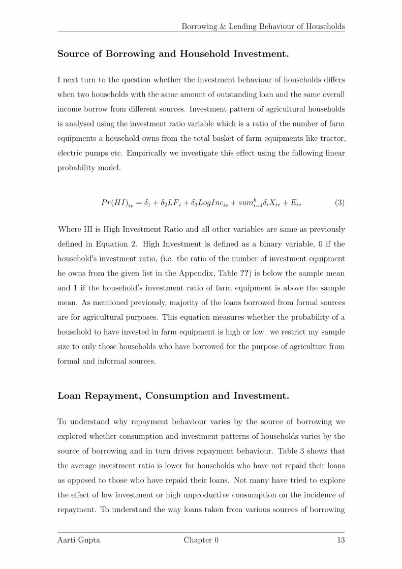
Pr(HI)iv = δ1 + δ2LF i + δ3LogInciv + sumki=4δiXiv + Eiv (3)

Where HI is High Investment Ratio and all other variables are same as previously

defined in Equation 2. High Investment is defined as a binary variable, 0 if the

household′s investment ratio, (i.e. the ratio of the number of investment equipment

he owns from the given list in the Appendix, Table ??) is below the sample mean

and 1 if the household′s investment ratio of farm equipment is above the sample

mean. As mentioned previously, majority of the loans borrowed from formal sources

are for agricultural purposes. This equation measures whether the probability of a

household to have invested in farm equipment is high or low. we restrict my sample

size to only those households who have borrowed for the purpose of agriculture from

formal and informal sources.

Loan Repayment, Consumption and Investment.

To understand why repayment behaviour varies by the source of borrowing we

explored whether consumption and investment patterns of households varies by the

source of borrowing and in turn drives repayment behaviour. Table 3 shows that

the average investment ratio is lower for households who have not repaid their loans

as opposed to those who have repaid their loans. Not many have tried to explore

the effect of low investment or high unproductive consumption on the incidence of

repayment. To understand the way loans taken from various sources of borrowing



are utilised by the households, we analyse how their investment and consumption

patterns have an effect on their repayment behaviour.

Pr(LR)iv = ε1 + ε2Pr(HSS)iv + ε3Pr(HI)ivε4logInciv + ε5Iriv + sumki=6εiXiv + Ei

(4)

where LR is Loan Repayment, HSS is High Social Spending, HI is High Investment

ratio, Ir is the monthly rate of interest payable by the household on the loan borrowed,

INC is log of income, Xi is a set of other covariates, such as, number of loans taken

by the household, largest amount of loan taken, household size, caste and religion.

Loan repayment, the dependent variable is a binary variable, 0 being if the household

has repaid its largest loan and 1 being if the household has not repaid its largest loan.

The ε2 coefficient records the increase in probability of loan repayment with every

percentage point increase in the probability to spend more on social functions than

the average.The ε3 coefficient records the increase in probability of loan repayment

with every percentage point increase in the probability to own more investment

equipment than the average.

Interest Rates

As mentioned before one of the objectives behind the introduction of formal banking

institutions in the rural areas by the government was to provide easy and cheap

access to credit. In the process the aim was to reduce dependence on money lenders

who charge high interest rates. However, the creation of institutional alternatives

has failed to drive the traditional money lender out of the market and the informal

interest rates remain high [Hoff and Stiglitz, 1990]. This raises the question as to how

interest rates play a role in the repayment behaviour of borrowers. Lower interest

rates can have important consequences on factors such as indebtedness, utilisation of

loan and repayment. The theoretical insight is that households can be induced to

take loan for income generating purposes, which in turn, can scale down debt burden

and enhance repayment when interest rate is low. An alternate possibility is that,

a high interest rate coupled with stricter monitoring of informal loans could push



the households towards defaulting less on the informal loans and as a consequence

default more on formal loans. To investigate these alternative possibilities we explore

how the behaviour of households differ when a high rate of interest is likely to alter

household’s ability to repay formal vs informal loans. we investigate this by looking

at the effect interest rates have on loan repayment when households borrow from

formal sources like banks as opposed to their effect on loan repayment when borrowed

from informal sources like money lenders.

The linear probability model below analyses how interest rates affect loan repayment

behaviour in general and do interest rates play a different role when households

borrow from formal sources of finance as opposed to informal sources.

Pr(LR)i = π1+π2SSi+π3Inci+π4Iri+π5Banki+π6Mli+sumki=7πiXi+Ei+xi (5)

Pr(LR)i = Π1+Π2SSi+Π3INCi+Π4Iri+Π5Banki+π6Bank ∗ Iri+sumki=7ΠiXi+Ei+qi

(6)

Pr(LR)i = ρ1 +ρ2SSi +ρ3INCi +ρ4Iri +ρ5Mli +ρ6Ml ∗ Iri +sumki=7ρiXi +Ei +oi

(7)

where LR is Loan Repayment, Bank is a dummy variable taking the value of 1, if a

household has borrowed the loan from a bank, and 0 otherwise. Ml is a dummy for

Money Lender, taking the value of 1, if a household has borrowed from a moneylender

and 0 otherwise. The Π6 coefficient in equation 7 is the interaction term of the

dummy variable Bank and monthly interest rate. It records the effect of monthly

interest rate on loan repayment when households borrow from Banks. Similarly ρ6

coefficient in equation 8 is the interaction term of the dummy variable moneylender

and monthly interest rate, which records the effect of monthly interest rate on loan



repayment when households borrow from moneylenders.

The next section looks at the results of these equations.

Results

Consumption

I start by investigating whether households with otherwise similar characteristics,

consume differently when borrowing the same amount of loan from formal vis-a-vis

informal sources. Consumption is measured as the monthly consumption per capita

for a household. It is calculated as a sum of total expenditures on 47 consumption

items on a monthly basis. For further details on the items included refer Table ??

in the Appendix. The results from the estimation of equation 1 are reported in

Table 4. Column-[1] reports the baseline estimates for α2 after controlling only for

household income. Since richer households are more likely to have greater access

to formal financial sector, and at the same time have higher consumption, hence it

is imperative that we control for income even in the very sparse specification. The

estimate suggests that, for similar level of total household income, if a household

has taken a loan from a formal source as opposed to an informal source then it is

likely to have a higher monthly consumption per capita by approximately Rs. 307

on average.

Column [2] additionally controls for household size, religion and caste. Previous

findings suggest that households from different socio economic background tend to

indulge more in consumption goods as a signalling mechanism [Khamis et al., 2012].

Hence we include religion and caste controls. The estimation suggests that even after

controlling for the additional variables there is a significant difference in consumption

expenditure of households depending on the source of their borrowing. Column [3],

additionally controls for village level fixed effects. It is possible that households living

in more developed regions have higher consumption expenditure simply because

of their access to various consumption goods. At the same time access to formal

finances are also likely to be higher in more developed regions. Village level fixed



effects ensures that we am comparing households with the same level of access to

formal finances. More generally it accounts for any difference in behaviour due to

unobserved heterogeneity across villages. Indeed, the importance of controlling for

village level development is evident from the estimate in Column [3]. Compared

to Column [1], the coefficient is almost halved. Households borrowing from formal

sources still have a higher level of consumption compared to households borrowing

from informal sources. However the difference is now approximately Rs 148.

Other control variables also have a significant effect. Loan size has a positive effect

on monthly per capita consumption. The results also suggest that Hindus have a

higher consumption as compared to other religions. OBC, ST and SC have lower

consumption as compared to households that belong to the General category of

caste. Column [4] estimates the same specification as Column [3] but we restrict

the sample to only those households who have borrowed for agricultural purposes.

These households have borrowed from either a formal source or an informal source,

specifically for the purpose of agricultural investment. The findings are similar

in spirit for these households. Specifically households which have borrowed for

agricultural investment purposes from a formal source as opposed to an informal

source spend Rs. 89 more per person in the house on consumption on a monthly

basis, indicating a higher monthly per capita consumption when a loan is taken

from a formal source as opposed to an informal source. Overall we find a significant

difference in consumption behaviour of households depending on the source from

which they borrowed their loans.

Social Spending

One reason for a higher per capita consumption could be that easier terms of formal

loans allow otherwise constrained households to spend on necessary and productive

consumption goods like food, education or health. This might lead to higher future

productivity of the households through human capital development. However, a more

worrisome possibility, from a policy perspective, is a higher extent of unproductive



Table 4: Effect of Borrowing Source on Monthly Consumption Per Capita

Dependent Variable - Monthly Consumption Per CapitaAll Loans Agricultural Loans

1 2 3 4

Loan Formal 306.3*** 236.7*** 131.5*** 76.87***(17.7) (17.6) (19.5) (29.0)

Income 289.3*** 251.9*** 151.7*** 126.6***(8.2) (8.2) (9.3) (14.1)

Loan Size 65.00*** 44.75*** 44.93***(3.8) (4.2) (7.5)

Brahmin 51.1 -5.0 -32.5(42.2) (47.1) (81.8)

OBC -267.4*** -191.0*** -149.1***(21.4) (26.3) (42.5)

ST -511.1*** -345.1*** -281.1***(35.2) (46.4) (75.5)

SC -382.1*** -342.9*** -341.0***(25.1) (29.4) (52.7)

Hindu 115.7*** 97.24*** 116.4**(23.1) (31.1) (53.8)

Constant 404*** 592*** 748*** 669***(14.6) (27.1) (33.4) (56.9)

PSU Fixed Effects No No Yes YesObservations 16785 16781 16781 5149R-squared 0.103 0.140 0.367 0.575

Notes. This table explores the impact of borrowing from formal source on monthly

consumption per capita of the household.The dependent variable COPC is the per capita

expenditure of a household on the list of 47 consumption items calculated for a monthly

period. Column [1] controls only for source of borrowing and income. In Column [2]

further control variables are added. Column[3] which is our preferred specification controls

for village level fixed effects in addition to the control variables in Column [2].Column

[4] explores the impact only on those households who have borrowed for the purpose

of agriculture. Data on all variables is taken from the IHDS 2009-10. Asterisks denote

significance: * p < :10, ** p < :05, *** p < :01. Standard errors are in brackets. Source:

IHDS 2004-05; Own Calculations.



spending that the households might indulge in when borrowing from formal sources.

To understand this further we look deeper into the composition of consumption. As

discussed earlier, households in India often consume goods that signal social status

even at the cost of nutrition and education. Hence in what follows we study whether

households tend to finance their expenditure on certain types of consumption by

taking advantage of the easier terms of formal loans. Specifically we focus here

on expenditure that are conspicuous in nature. Conspicuous consumption is easily

visible to others and hence more likely to help households in signalling their social

status.

The results from the estimation of equation 2 are reported in Table 5. The dependent

variable High Social Spending is a binary variable which takes the value 1 when the

household′s social spending is higher than the average (Rs 2922) and 0, otherwise.

The reason for not using a continuous variable for social spending is that a large

number of households report zero social spendings. Column [1] reports the baseline

estimates for β2, after controlling for household income. The estimate suggests that

for similar levels of total household income, if a household has taken a loan from a

formal source as opposed to an informal source then it is likely to have a 5% higher

probability of indulging in higher social spending.

Column [2] additionally controls for household size, loan size, religion and caste.

This lowers the size of the coefficient, but it still remains significant. Column [3]

additionally controls for village level fixed effects. After controlling for the unobserved

differences at the village level the probability of having a higher social spending

when a loan is borrowed from a formal source is about 2% higher compared to when

a loanis borrowed from an informal source.

Column[4] estimates the same specification as Column[3] but with a restricted sample

size of only loans which have been taken for agricultural purposes. It is interesting

to see that households who take loans for agricultural investments from formal

sources as opposed to informal sources have a 4% higher probability of indulging

in higher social spending. This is indicative of a presence of moral hazard in the

utilisation of loans from formal sources and specifically those taken for agricultural

use. Households may form expectations that either monitoring or enforcement of



loans by formal sources is not strong and thus exercise less control in utilisation of

these loans. The fact that the unproductive agricultural loans have almost double

the effect of any formal loan, might further reflect the fact that loan waivers are

specifically targeted towards agricultural loans which change people′s expectations

about the terms of enforcement of these loans in particular.

Investment Ratio

Credit has always been looked at as a facilitator for modernising agriculture. At a

basic level credit serves as a means to remove financial constraint. But the bigger role

of credit in agriculture is to help farmers create assets that can help generate output

by adopting modern means of technology. Thus it is very important for households

to utilise the agricultural loan taken for investment purposes. By utilising loans for

investment purposes whether it is in the form of buying a tractor or setting up tube

wells, it helps in modernising the farm and eventually helps increase productivity. By

adequately investing in production and technology farmers can achieve farm income

sustainability and consumption stability. However given that the overall budget is

constrained by the loan amount, an increase in consumption expenditure is likely to

bring down productive expenditure. Hence in what follows we study the investment

made by households who borrow from formal sources as opposed to informal sources.

The results from the estimation of equation 3 are reported in Table 2.6. High

Investment Ratio is a binary variable which takes the value 1 when the household′s

investment ratio (fraction of investment goods owned by the household out of 7 total

investment goods) is more than the average investment ratio and 0, otherwise 1. The

primary objective of this thesis is to study loan waivers and behaviours of households

in the context of agriculture. we restrict the sample size for this analysis to only

agricultural loans as studying investment ratios for loans taken for other purposes is

meaningless in this context. Column [1] reports the baseline estimates forβ2, after

controlling for household income. The estimate suggests that for similar level of total

1The average investment ratio of the entire sample if 0.0974.



Table 5: Effect of Borrowing Source on Social Spending

Dependent Variable -Pr (High Social Spending)All Loans Agricultural Loans

1 2 3 4

Loan Formal 0.046*** 0.034*** 0.019*** 0.041***(0.006) (0.006) (0.007) (0.012)

Income 0.054*** 0.043*** 0.051*** 0.046***(0.003) (0.003) (0.003) (0.006)

HH Size 0.012*** 0.010*** 0.012***(0.001) (0.001) (0.002 )

Loan Size 0.009*** 0.007*** 0.007**(0.001) (0.001) (0.003)

Brahmin 0.055*** 0.033** -0.006(0.014) (0.016) (0.035)

OBC -0.031*** -0.042*** -0.077***(0.007) (0.009) (0.018)

ST -0.060*** -0.063*** -0.062*(0.012) (0.016) (0.032)

SC -0.059*** -0.072*** -0.134***(0.008) (0.01) (0.023)

Hindu 0.016** 0.014 0.026(0.008 ) (0.011) (0.023)

Constant 0.050*** 0.015 0.031** 0.029(0.005) (0.01) (0.012) (0.026)

PSU Fixed Effects No No Yes YesObservations 16,785 16,781 16,781 5,149R-squared 0.033 0.049 0.285 0.457

Notes. This table explores the impact of borrowing from formal source on the social

spending of the household.The dependent variable is social spending, which is a binary

variable. It is 1 when a household spends more than the mean amount on social functions

and 0 otherwise. Column [1] controls only for source of borrowing and income. In Column [2]






IHDS 2004–2005, own calculations.



household income, if a household has taken a loan from a formal source as opposed

to an informal source then it is likely to have a 5.2% higher probability of investing

in more than the average investment.

Column [2] additionally controls for household size, loan size, religion and caste.

Column [3] additionally controls for village level fixed effects. After controlling for

the unobserved differences at the village level the probability of having a higher

investment ratio when a loan is borrowed from a formal source goes up to .5%.

This is the expected sign of investment ratio and borrowing from formal source

indicating no moral hazard. However the interesting analysis comes in Column[4],

which estimates the same specification as Column[3] but with a restricted sample

size to only those households which have a high social spending. Here we notice

that households which spend high amounts on social events and borrow from formal

sources have a 13.6% lower probability of having a high investment ratio. This is

indicative of a presence of moral hazard in the utilisation of loans from formal sources

taken for agricultural purposes suggesting that households divert the funds borrowed

for investment purposes towards unproductive purposes.

Loan Repayment

Utilisation of loans plays a very important role in the repayment of loans. If a loan

is used for income generating purposes then it generates income and increases the

overall sustainability of the household. On the other hand if the loan is used for

unproductive purposes then the loan becomes a burden on the household as is likely

to create a vicious debt trap. Hence in what follows we investigate whether low

investment ratio and/or high social spending impacts loan repayment of households.

The results from the estimation of equation 4 are reported in Table 2.7. Loan

Repayment is a binary variable which takes the value 1 when a household has repaid

its loan and 0, otherwise.

Column [1] reports the baseline estimates for ε2 in equation 4, after controlling

household income, monthly interest rate, loan size, household size, caste and religion



Table 6: Effect of Borrowing Source on Investment Ratio

Dependent Variable -Pr (High Investment Ratio)Agri Loans Agri Loans with HSS

1 2 3 4

Loan Formal 0.052*** 0.038** 0.065*** -0.136**(0.017 ) (0.017) (0.02) (0.068 )

Income 0.088*** 0.058*** 0.050*** 0.029(0.008) (0.008) (0.01) (0.03)

HH Size 0.022*** 0.022*** 0.015(0.003) (0.003) (0.009)

Loan Size 0.027*** 0.026*** 0.015(0.005) (0.005) (0.025)

Brahmin -0.102** -0.028 -0.003(0.046) (0.061) (0.195)

OBC -0.089*** -0.044 -0.074(0.021) (0.031) (0.092)

ST -0.162*** -0.131*** -0.168(0.032 ) (0.05) (0.18)

SC -0.178*** -0.181*** -0.009(0.029) (0.039) (0.146)

Hindu 0.107*** 0.140*** 0.076-0.027 -0.04 -0.165

Constant 0.415*** 0.306*** 0.241*** 0.603***(0.015 ) (0.033) (0.045) (0.155)

PSU Fixed Effects No No Yes YesObservations 3,429 3,429 3,429 558R-squared 0.04 0.078 0.534 0.735

Notes. This table explores the impact of borrowing from formal source on the investment

ratio of the household.The dependent variable is social spending, which is a binary variable.

It is 1 when a household spends more than the mean amount on social functions and 0

otherwise. Column [1] controls only for source of borrowing and income. In Column [2]






IHDS 2004-05



dummies and the number of loans taken in the last 5 years. In addition it controls

for village level fixed effects. The estimate suggests that for similar level of total

household income and loan size if a household has high social spending then its

probability to default will increase by 1.7%.

Column [2] uses the same specification as column [1], but the sample size is restricted

to only agricultural loans. In this specification, we see a drastic increase in default

rate to 5.3% when a household has a higher social spending as opposed to one

having a low social spending. Column [3] reports the baseline estimates for ε3, after

controlling household income, monthly interest rate, loan size, household size, caste

and religion dummies and the number of loans taken in the last 5 years. In this

specification, after controlling for the unobserved differences at the village level,

households which have a high investment ratio have a 3.2% lower probability of

default although the coefficient is significant only at 16% confidence level.

Since the household is likely to be faced by a resource constraint a higher level of

social spending might crowd out investment spending, instead of reducing other

forms of consumption expenditure. To investigate the possibility Column [4] includes

both social spending and investment spending in the same specification. The results

suggest that a higher that average expenditure on social functions reduces the

probability of repaying the loan borrowed by 5%. On the other hand a higher

than average expenditure on investment increases the probability of repaying the

loan borrowed by 3.4%. This suggests that there is a possibility that increasing

expenditure on social functions is reducing the ability of the household to repay their

loan.

Interest Rate

To avoid wilful default on the part of the borrowers, lending agencies both formal

and informal impose penalties in case of default. Penalties are generally in the

form of seizing collateral or discontinuing future credit availability. Bhattacharjee

[2014] argue that penalty could also be levied through interest rates charges on

loans. Specifically they examine the impact of interest rate in the informal sector on

formal sector repayment. They find that a higher unfavourable interest rate in the



Table 7: Effect of Social Spending & Investment Ratio of Loan Repayment

Dependent Variable - Pr (Loan Repayment)( 1) (2 )

Bank * Monthly Interest -0.080***(0.021)

MoneyLender * Monthly Interest 0.029***(0.004)

Pr(High Social Spending) 0.026*** 0.026***(0.01) (0.01)

Income 0.009*** 0.010***(0.004) (0.004)

Monthly Interest -0.019*** -0.031***(0.002) (0.003)

Bank 0.005 0.104***(0.009) (0.024)

MoneyLender -0.118***(0.013)

HH Size -0.003** -0.003**(0.001) (0.001)

Brahmin -0.005 -0.006(0.018) (0.018)

OBC -0.053*** -0.050***(0.009) (0.009)

ST 0.013 0.014(0.015) (0.015)

SC -0.048*** -0.044***(0.011) (0.011)

Loan Size -0.001 -0.001(0.002) (0.002)

Hindu -0.030*** -0.025**(0.01) (0.01)

Constant 0.365*** 0.391***(0.014) (0.014)

PSU Fixed Effects Yes YesObservations 16,773 16,773R-squared 0.018 0.021

Notes. This table explores the impact of interest rates charged on loans borrowed by

formal and informal sources, in particular banks and money lenders on the loan repayment

probability of a household.The dependent variable is loan repayment, which is a binary

variable. It is 1 when a household has repaid the loan and 0, otherwise. Column [1] shows

the effect of high social spending on loan repayment controlling for other variables for all

loans. In Column[2],[3] and [4] the sample size is restricted to only agricultural households.

Column [2] shows the effect of high social spending on loan repayment, Column [3] shows

the effect of high investment ratio on loan repayment and Column [4] shows the effect of

both high social spending and high investment ratio on probability of loan repayment. All

regressions control for village level fixed effects. Asterisks denote significance: * p < :10,

** p < :05, *** p < :01. Standard errors are in brackets. Source: IHDS 2004-05, Own

Calculation



informal sector leads to an increase in timely repayment in the formal sector. To add

to this finding, we estimate the effect that interest rates have on loan repayment,

specifically in the case of agricultural loans where expected penalty might vary from

actual penalty due to frequent announcement of loan waiver programs, The results

from the estimation of equation 7 are reported in Table 8. Loan Repayment is a

binary variable which takes the value 1 when a household has repaid its loan and

0, otherwise. In this specification we use Banks as a proxy for formal loans as they

formulate majority of the formal loans and moneylenders as a proxy for informal

loans.

Column [1] reports the baseline estimates for π6, after controlling household income,

monthly interest rate, loan size, household size, caste and religion dummies. The

interaction term [Bank * Monthly interest) implies that when a household borrows

from a bank as opposed to any other lending agency, a higher interest rate reduces

the probability of loan repayment by 8%. On the other hand Column [3] shows the

effect on loan repayment when a household borrows from a moneylender. In this case,

a higher interest rates on moneylender loans increases the probability of repayment

by approximately 3%.

In this case a higher interest rate on loans from formal institutions make household

default more. This could simply be driven by a larger size of debt as a result of higher

interest rate. Especially if the fear of losing credit worthiness is low people will tend

to default more when debt size is large. On the other hand, the fear of losing future

credit possibility in case of default is always high for the informal loans, which run

precisely on the basis of reputation. Further if credit worthiness is a function of the

debt size itself, so that a reputation is at a greater stake, larger the size of default,

then people would be more likely to return informal debts when they are larger in

size due to a higher interest rate.



Table 8: Effect of Interest Rate on Loan Repayment

Dependent Variable - Pr (Loan Repayment)( 1) (2 )

Bank * Monthly Interest -0.080***(0.021)

MoneyLender * Monthly Interest 0.029***(0.004)

Pr(High Social Spending) 0.026*** 0.026***(0.01) (0.01)

Income 0.009*** 0.010***(0.004) (0.004)

Monthly Interest -0.019*** -0.031***(0.002) (0.003)

Bank 0.005 0.104***(0.009) (0.024)

MoneyLender -0.118***(0.013)

HH Size -0.003** -0.003**(0.001) (0.001)

Brahmin -0.005 -0.006(0.018) (0.018)

OBC -0.053*** -0.050***(0.009) (0.009)

ST 0.013 0.014(0.015) (0.015)

SC -0.048*** -0.044***(0.011) (0.011)

Loan Size -0.001 -0.001(0.002) (0.002)

Hindu -0.030*** -0.025**(0.01) (0.01)

Constant 0.365*** 0.391***(0.014) (0.014)

PSU Fixed Effects Yes YesObservations 16,773 16,773R-squared 0.018 0.021

Notes. This table explores the impact of interest rates charged on loans borrowed by

formal and informal sources, in particular banks and money lenders on the loan repayment

probability of a household.The dependent variable is loan repayment. Column[1] shows us

the interaction term [Bank*Monthly interest], which captures the effect of interest rates

charged by the bank on probability of loan repayment. Column[2] shows us the effect of

interest rates charged by moneylenders on probability of loan repayment.Asterisks denote


IHDS 2004-05; Own Calculations



Conclusion

Repayment of loans depends on a number of factors, such as purpose for which loan

is taken, tenure of the loan, interest rate and source of borrowing. If a household

borrows a loan meant for income generating purpose and uses it for that then it is

likely to generate future income and make the household better off in the long run.

It is also likely to enable the household to return the loan borrowed in the first place.

However, if the loan is used for unproductive purposes, then repaying that loan

becomes problematic for the household. The household can then get stuck in a debt

trap where it borrows more to repay the previous loan and the economic status of the

household does not improve. Even if households are aware of this and avoid using

investment loans for consumption purposes in general, government interventions in

the form of loan waivers might change the behaviour of households.

Moral hazard might arise when government intervene and announce loan waiver

policies. Households which could have avoided using their loans for consumption

purposes also have an incentive to default. It encourages people to be less cautious in

using their loans for non productive purposes in the hope that there will be further

loan waiver announcements and the punishment for default will be low.

In this chapter we explored the consumption, investment and loan repayment be-

haviour of households that borrow loans from formal sources as opposed to informal

sources. Empirical results suggest that households that borrow from formal sources

have a higher consumption and social spending. They expenditure on investment

products are also lesser than the average. In addition to this we also find that

households that have a higher than average expenditure on social spending have a

lower probability of repaying their loans. This implies that households which borrow

from formal sources spend more on social functions as compared to households that

borrow from informal sources and thus have a lesser probability of repaying their

loans as they have used the borrowed loan amount for unproductive expenditure.


Bibliography

Abhijit V Banerjee and Esther Duflo. The economic lives of the poor. The journal

of economic perspectives, 21(1):141–167, 2007.

Timothy Besley. Savings, credit and insurance. Handbook of development economics,

3:2123–2207, 1995.

Manojit Bhattacharjee. Indebtedness in the household sector. A study of selected

states in India. PhD thesis, 2014.

Robin Burgess and Rohini Pande. Can rural banks reduce poverty? evidence from

the indian social banking experiment. American Economic Review, 2004.

Robin Burgess, Rohini Pande, and Grace Wong. Banking for the poor: Evidence

from india. Journal of the European Economic Association, 3(2-3):268–278, 2005.

Erica Field and Rohini Pande. Repayment frequency and default in microfinance:

evidence from india. Journal of the European Economic Association, 6(2-3):

501–509, 2008.

Parikshit Ghosh, Dilip Mookherjee, and Debraj Ray. Credit rationing in develop-

ing countries: an overview of the theory. Readings in the theory of economic

development, pages 383–401, 2000.

Xavier Gine, Karuna Krishnaswamy, and Alejandro Ponce. Strategic default in joint

liability groups: Evidence from a natural experiment in india. 2013.

Anwarul Hoda and Prerna Terway. Credit policy for agriculture in india-an evaluation.

Indian Council For Research On International Economic Relations, 2015.

29


Karla Hoff and Joseph E Stiglitz. Introduction: Imperfect information and rural

credit markets: Puzzles and policy perspectives. The world bank economic review,

pages 235–250, 1990.

Martin Kanz. What does debt relief do for development? evidence from india’s

bailout program for highly-indebted rural households. Evidence from India’s

Bailout Program for Highly-Indebted Rural Households (November 1, 2012). World

Bank Policy Research Working Paper, (6258), 2012.

Melanie Khamis, Nishith Prakash, and Zahra Siddique. Consumption and social

identity: Evidence from india. Journal of Economic Behavior & Organization, 83

(3):353–371, 2012.

Paul Krugman. Financing vs. forgiving a debt overhang. Journal of development

Economics, 29(3):253–268, 1988.

Andreas Madestam. Informal finance: A theory of moneylenders. Journal of

Development Economics, 107:157–174, 2014.

Srijit Mishra. Farmers’ suicides in maharashtra. Economic and Political Weekly,

pages 1538–1545, 2006.

Biswa Swarup Misra et al. The performance of regional rural banks (rrbs) in india:

Has past anything to suggest for future. Reserve bank of India occasional papers,

27(1):89–118, 2006.

K Nagaraj. Farmers’ suicides in India: Magnitudes, trends and spatial patterns.

Bharathi Puthakalayam, 2008.

Sarmistha Pal. Household sectoral choice and effective demand for rural credit in

india. Applied Economics, 34(14):1743–1755, 2002.

Narayan Chandra Pradhan. Persistence of informal credit in rural india: Evidence

from ‘all-india debt and investment survey and beyond. Reserve Bank of India

(RBI) working paper, 5, 2013.

Meenakshi Rajeev and HP Mahesh. banking sector reforms and npa: a study of

indian commercial banks. 2010.



RBI. Handbook of statistics on indian economy, 2014.

Jeffrey Sachs. The debt overhang of developing countries in debt stabilisation and

development: Essays in memory of carlos diaz alejandro, ed. by guillermo calco

and others. 1989.

Mudita Tiwari. What was the Agricultural Debt Waiver and Debt

Relief Scheme about? http://www.developmentoutlook.org/2012/10/

what-was-agricultural-debt-waiver-and.html, 2012. [Online; accessed 1-

april-2014].

Robert M Townsend and Kenichi Ueda. Financial deepening, inequality, and growth:

A model-based quantitative evaluation. Number 3-193. International Monetary

Fund, 2003.

John D Von Pischke, Dale W Adams, and Gordon Donald. Rural financial markets

in developing countries. Johns Hopkins, 1983.


http://www.developmentoutlook.org/2012/10/what-was-agricultural-debt-waiver-and.html

http://www.developmentoutlook.org/2012/10/what-was-agricultural-debt-waiver-and.html

loan repayment behaviour of farmers: analysing...

Documents