Local Distribution and the Symmetry Gap:

Approximability of Multiway Partitioning Problems∗

Alina Ene† Jan Vondrak‡ Yi Wu§

Abstract

We study the approximability of multiway partitioning problems, examples of which includeMultiway Cut, Node-weighted Multiway Cut, and Hypergraph Multiway Cut. We investigate theseproblems from the point of view of two possible generalizations: as Min-CSPs, and as SubmodularMultiway Partition problems. These two generalizations lead to two natural relaxations, the BasicLP, and the Lovasz relaxation. The Basic LP is generally stronger than the Lovasz relaxation, butgrows exponentially with the arity of the Min-CSP. The relaxations coincide in some cases such asMultiway Cut where they are both equivalent to the CKR relaxation.

We show that the Lovasz relaxation gives a (2− 2/k)-approximation for Submodular MultiwayPartition with k terminals, improving a recent 2-approximation [4]. We prove that this factor isoptimal in two senses: (1) A (2− 2/k− ε)-approximation for Submodular Multiway Partition withk terminals would require exponentially many value queries. (2) For Hypergraph Multiway Cutand Node-weighted Multiway Cut with k terminals, both special cases of Submodular MultiwayPartition, we prove that a (2 − 2/k − ε)-approximation is NP-hard, assuming the Unique GamesConjecture.

Both our hardness results are more general: (1) We show that the notion of symmetry gap,previously used for submodular maximization problems [24, 8], also implies hardness results forsubmodular minimization problems. (2) Assuming the Unique Games Conjecture, we show thatthe Basic LP gives an optimal approximation for every Min-CSP that includes the Not-Equalpredicate.

Finally, we connect the two hardness techniques by proving that the integrality gap of theBasic LP coincides with the symmetry gap of the multilinear relaxation (for a related instance).This shows that the appearance of the same hardness threshold for a Min-CSP and the relatedsubmodular minimization problem is not a coincidence.

1 Introduction

In this paper, we study the approximability of multiway cut/partitioning problems, where a groundset V should be partitioned into k parts while minimizing a certain objective function. Classicalexamples of such problems are Multiway Cut (that we abbreviate by Graph-MC), Node-weightedMultiway Cut (Node-Wt-MC) and Hypergraph Multiway Cut (Hypergraph-MC). These problemsare NP-hard but admit constant-factor approximations.

∗This is a full version of the paper that appeared in ACM-SIAM SODA 2013 [9].†Department of Computer Science, University of Illinois at Urbana-Champaign. Supported in part by NSF grants

CCF-0728782 and CCF-1016684. Part of this work was done while the author was visiting the IBM Almaden ResearchCenter.‡IBM Almaden Research Center, San Jose, CA§Department of Computer Science, Purdue University. Part of this work was done while the author was a postdoc at

the IBM Almaden Research Center.

1

Multiway Cut (Graph-MC): Given a graph G = (V,E) with weights on the edges and k terminalst1, t2, . . . , tk ∈ V , remove a minimum-weight set of edges so that every two terminals are disconnected.

Node-weighted Multiway Cut (Node-Wt-MC): Given a graph G = (V,E) with weights on thenodes and k terminals t1, t2, . . . , tk ∈ V , remove a minimum-weight set of vertices so that every twoterminals are disconnected.

Hypergraph Multiway Cut (Hypergraph-MC): Given a hypergraph H = (V,E) with weights onthe hyperedges and k terminals t1, t2, . . . , tk ∈ V , remove a minimum-weight set of hyperedges so thatevery two terminals are disconnected.

Although the problems above are formulated as vertex/edge/hyperedge removal problems, Graph-MC and Hypergraph-MC can be also viewed as partitioning problems where vertices are assignedto terminals and we pay for each edge/hyperedge that is cut between different terminals. The Node-Wt-MC problem can also be stated in this form, and in fact shown to be approximation-equivalent toHypergraph-MC (although the reduction is more complicated, see [19]). Given this point of view,and the fact that the cut function in graphs/hypergraphs is submodular, the following generalizationof these problems was proposed in [26] and recently studied in [5, 4].

Submodular Multiway Partition (Sub-MP): Given a submodular set function f : 2V → R+ andk terminals t1, t2, . . . , tk ∈ V , find a partition of V into A1, . . . , Ak such that ti ∈ Ai and

∑ki=1 f(Ai)

is minimized.

This problem captures the problems Graph-MC, Node-Wt-MC and Hypergraph-MC as spe-cial cases.1 One of the useful aspects of viewing the problems in this more general framework isthat non-trivial linear programs, discovered on a case-by-case basis in the past, can be viewed in aunified way: by considering the Lovasz extension of a submodular function (see Section 2 for details).In particular, [5] rederives the geometric CKR relaxation for Multiway Cut [2] in this way. It wasshown in [4] that Sub-MP is not significantly more difficult than its special cases: Sub-MP admits a2-approximation in general, and an improved (3/2 − 1/k)-approximation when the number of termi-nals is k and f is a symmetric submodular function (in the sense that f(S) = f(S); we denote thisspecial case as Sub-MP-Sym). We remark that Graph-MC is a special case of Sub-MP-Sym, whileNode-Wt-MC and Hypergraph-MC are not.

This compares to the approximability of the classical problems as follows: Graph-MC admits a1.2965-approximation, which has been obtained by a sequence of successive improvements [2, 12, 1, 21],all based on the CKR relaxation of [2]. The (3/2 − 1/k)-approximation obtained by [2] matchesthe result of [4] for Sub-MP-Sym. On the hardness side, it was proved that the CKR relaxationprovides the optimal approximation factor for Graph-MC, assuming the Unique Games Conjecture[17]. However, the actual approximation factor is not known: it is only known that it is between 8/7and 1.2965. In the case of 3 terminals, the optimal factor is known to be 12/11 [12, 17].

The problems Node-Wt-MC and Hypergraph-MC are known to be approximation-equivalent,and both admit a (2 − 2/k)-approximation for k terminals [19, 10]. It is known that a (2 − ε)-approximation independent of k would imply a (2− ε)-approximation for Vertex Cover, which wouldrefute the Unique Games Conjecture. Therefore, we do not expect an approximation better than2 for Node-Wt-MC and Hypergraph-MC when the number of terminals is large. Nevertheless,this reduction does not give any hardness for a constant number of terminals k, and the optimalapproximation for a given k was not known.

1We point out that in the case of Hypergraph-MC, the reduction is not as direct as one might expect - this isdue to the fact that we want to count each cut hyperedge only once, independently of how many terminals share it.Consequently, the arising submodular function is not symmetric, although the cut function in a hypergraph is.

2

Our contribution. We study these partitioning problems from two points of view: (a) as generalpartitioning problems with a submodular cost function, using a natural convex program for the problembased on the Lovasz extension of a submodular function; we refer to this convex program as the Lovaszrelaxation; (b) regarding them as Min-CSPs (constraint satisfaction problems), which leads to anothernatural relaxation that has been referred to as the Basic LP (see, e.g., [14, 22]).2 Our concrete resultsare as follows.

Concrete results:

• We give a (2− 2/k)-approximation for the Sub-MP problem with k terminals using the Lovaszrelaxation. We also show that this is optimal, in two different senses.

• We prove that any (2−2/k− ε)-approximation for Sub-MP (for a constant number of terminalsk) requires exponentially many value queries in the oracle model.

• We prove that for Node-Wt-MC, a special case of Sub-MP, it is Unique-Games-hard to achievea (2− 2/k − ε)-approximation (for a constant number of terminals k).

Since Hypergraph-MC is approximation-equivalent to Node-Wt-MC, we determine the approx-imability of all three problems, Sub-MP, Hypergraph-MC and Node-Wt-MC, to be exactly 2−2/k(assuming the Unique Games Conjecture in the case of Hypergraph-MC and Node-Wt-MC).

Unique Games-hardness vs. NP-hardness more generally: Our hardness proofs in fact leadto more general results, revealing an interesting relationship between the Unique Games-hardness ofMin-CSP problems and NP-hardness of their natural submodular generalizations.

• We show a Unique Games-based hardness result for Min-CSP problems, generalizing the ma-chinery of [17]. Roughly speaking, we show that for every Min-CSP problem that includesthe Not-Equal predicate, the integrality gap of the Basic LP can be translated to a UniqueGames-hardness result.

• We show how the symmetry gap technique, previously developed for submodular maximizationproblems [24], applies to submodular minimization problems. This technique yields hardness re-sults in the value oracle model, or computational hardness assuming NP 6= RP , using the tech-nique of [8]. In particular, we prove that it is hard to achieve a better than 1.268-approximationfor Sub-MP-Sym (a special case of Sub-MP where the cost function is symmetric submodular).

Finally, we present a connection between the two approaches, proving that the integrality gap of theBasic LP coincides with the symmetry gap of the multilinear relaxation (see the discussion below andSection 6 for more details).

Discussion. Let us comment on some connections that we observed here.Integrality gap vs. symmetry gap. While Unique Games-hardness results typically start from anintegrality gap instance, hardness results for submodular functions often start from the multilinearrelaxation of a problem, exhibiting a certain symmetry gap (see [24, 8]). This is a somewhat differentconcept, where instead of integral vs. fractional solutions, we compare symmetric vs. asymmetricsolutions. In this paper, we clarify the relationship between the two: For any integrality gap Min-CSPinstance of the Basic LP, there is a related Min-CSP instance that exhibits the same symmetry gapin its multilinear relaxation. Conversely, for any symmetry gap instance of the multilinear relaxationof a Min-CSP instance, there is a related Min-CSP instance whose Basic LP has the same integralitygap (see Section 6). Therefore, the two concepts are in some sense equivalent (at least for Min-CSP

2In the ACM-SIAM SODA 2013 version of this paper, we referred to this LP as Local Distribution LP.

3

problems). This explains why the Unique Games-hardness threshold for Hypergraph-MC and theNP-hardness threshold for its submodular generalization Sub-MP are the same.Lovasz vs. multilinear relaxation. The fact that the symmetry gap technique gives optimal results fora submodular minimization problem is interesting: The symmetry gap technique is intimately tied tothe notion of a multilinear extension of a submodular function, which has recently found numerousapplications in maximization of submodular functions [23, 24, 13, 15, 6]. Nevertheless, it has beencommon wisdom that the Lovasz extension is the appropriate extension for submodular minimization[16, 11, 5, 4]. Here, we obtain a positive result using the Lovasz extension, and a matching hardnessresult using the multilinear extension.

Erratum. In the conference version [9], it was claimed that for every fixed k ≥ 1 and ε > 0 there isan efficient algorithm to round the Basic LP for a Min k-CSP instance, achieving an approximationfactor within ε of the integrality gap. This result was found to contain errors and has been removed.

Organization. The rest of the paper is organized as follows. In Section 2, we discuss the Lovaszrelaxation, and show how it yields a (2− 2/k)-approximation for the Sub-MP problem. In Section 3,we present the symmetry gap technique for submodular minimization problems, and show how itimplies our hardness results in the value oracle model. In Section 4, we present our hardness result forMin-CSP, and show how it implies the hardness result for Hypergraph-MC. In section 5, we discussthe relationship of the Lovasz relaxation and the Basic LP. In Section 6, we discuss the relationshipof integrality gaps and symmetry gaps.

2 Approximation for Submodular Multiway Partition

In this section, we revisit the convex relaxation proposed by Chekuri and Ene [5], and provide animproved analysis that gives the following result.

Theorem 2.1. There is a polynomial-time (2− 2/k)-approximation for the Sub-MP problem with kterminals, where k and the terminals t1, . . . , tk are given on the input and the cost function is givenby a value oracle.

The Lovasz relaxation. The following is the convex relaxation that has been used by Chekuri andEne:

(SubMP-Rel) min∑k

i=1 f(xi) :

∀j ∈ V ;∑k

i=1 xi,j = 1;

∀i ∈ [k]; xi,ti = 1;

∀i, j; xi,j ≥ 0.

Here, f(xi) denotes the Lovasz extension of a submodular function. The function f can be definedin several equivalent ways (see [5, 4]). One definition is based on the following rounding strategy. Wechoose a uniformly random θ ∈ [0, 1] and define Ai(θ) = j : xij > θ. Then f(xi) = E[f(Ai(θ))].

Equivalently (for submodular functions), f is the convex closure of f on [0, 1]V . The second defini-tion shows that the relaxation SubMP-Rel is a convex program and therefore it can be solved inpolynomial time.

Given a fractional solution, we use the following randomized rounding technique, a slight modifi-cation of one proposed by Chekuri and Ene:

Randomized rounding for the Lovasz relaxation.

4

• Choose θ ∈ (12 , 1] uniformly at random and define Ai(θ) = j : xij > θ.

• Define U(θ) = V \⋃ki=1Ai(θ) = j : maxi xij ≤ θ.

• Allocate each Ai(θ) to terminal i, and in addition allocate U(θ) to a terminal i′ chosen uniformlyat random.

Each terminal ti is allocated to itself with probability one. Moreover, the sets Ai(θ) are disjointby construction, and therefore the rounding constructs a feasible solution. The only difference fromChekuri and Ene’s rounding [4] is that we assign the “unallocated set” U(θ) to a random terminalrather than a fixed terminal. (However, taking advantage of this in the analysis is not straightforward.)We prove the following.

Theorem 2.2. The above rounding gives a feasible solution of expected value at most (2− 2k )∑k

i=1 f(xi).

This implies Theorem 2.1. In the following, we prove Theorem 2.2. We assume that f(∅) = 0.This is without loss of generality, as the value of the empty set can be decreased without violatingsubmodularity and this does not affect the problem (since terminals are always assigned to themselves).

We start by defining several sets, parameterized by θ, that will be important in the analysis.

• Ai(θ) = j : xij > θ

• A(θ) =⋃ki=1Ai(θ) = j : maxi xij > θ

• U(θ) = V \A(θ) = j : maxi xij ≤ θ.

• B(θ) = U(1− θ) = j : 1−maxi xij ≥ θ.

We can express the LP cost and the cost of the rounded solution in terms of these sets as follows.The following lemma follows immediately from the definition of the Lovasz extension.

Lemma 2.3. The cost of the LP solution is

LP =

k∑i=1

∫ 1

0f(Ai(θ))dθ.

The next lemma gives an expression for the expected value achieved by the algorithm in a formconvenient for the analysis.

Lemma 2.4. The expected cost of the rounded solution is

ALG =

(2− 2

k

) k∑i=1

∫ 1

1/2f(Ai(θ))dθ +

2

k

k∑i=1

∫ 1/2

0f(Ai(θ) ∪B(θ))dθ.

Proof. The set allocated to terminal i is Ai(θ) with probability 1 − 1/k, and Ai(θ) ∪ U(θ) withprobability 1/k. We are choosing θ uniformly between 1

2 and 1. This gives the expression

ALG =

(2− 2

k

) k∑i=1

∫ 1

1/2f(Ai(θ))dθ +

2

k

k∑i=1

∫ 1

1/2f(Ai(θ) ∪ U(θ))dθ.

We claim that for θ ∈ [12 , 1], Ai(θ) ∪ U(θ) can be written equivalently as Ai(1 − θ) ∪ B(1 − θ). We

consider three cases for each element j:

5

• If xij >12 , then j ∈ Ai(θ) ∪ U(θ) for every θ ∈ [1

2 , 1], because xi′j <12 for every other i′ 6= i and

hence j cannot be allocated to any other terminal. Similarly, j ∈ Ai(1− θ) ∪B(1− θ) for everyθ ∈ [1

2 , 1], because 1− θ ≤ 12 and so j ∈ Ai(1− θ).

• If xij ≤ 12 and xij = maxi′ xi′j , then again j ∈ Ai(θ) ∪ U(θ) for every θ ∈ [1

2 , 1], because j isalways in the unallocated set U(θ). Also, j ∈ Ai(1− θ) ∪B(1− θ), because B(1− θ) = U(θ).

• If xij ≤ 12 and xij < maxi′ xi′j , then j ∈ Ai(θ) ∪ U(θ) if and only if j ∈ U(θ) = B(1− θ). Also,

we have xij = 1−∑

i′ 6=i xi′j ≤ 1−maxi′ xi′j , and therefore j ∈ Ai(1− θ) ∪B(1− θ) if and onlyif j ∈ B(1− θ).

To summarize, for every θ ∈ [12 , 1], j ∈ Ai(θ) ∪ U(θ) if and only if j ∈ Ai(1 − θ) ∪ B(1 − θ).

Therefore, the total expected cost can be written as

ALG =

(2− 2

k

) k∑i=1

∫ 1

1/2f(Ai(θ))dθ +

2

k

k∑i=1

∫ 1

1/2f(Ai(θ) ∪ U(θ))dθ

=

(2− 2

k

) k∑i=1

∫ 1

1/2f(Ai(θ))dθ +

2

k

k∑i=1

∫ 1

1/2f(Ai(1− θ) ∪B(1− θ))dθ

=

(2− 2

k

) k∑i=1

∫ 1

1/2f(Ai(θ))dθ +

2

k

k∑i=1

∫ 1/2

0f(Ai(θ) ∪B(θ))dθ.

In the rest of the analysis, we prove several inequalities that relate the LP cost to the ALG cost.Note that the integrals

∫ 11/2 f(Ai(θ))dθ appear in both LP and ALG. The non-trivial part is how to

relate∫ 1/2

0 f(Ai(θ))dθ to∫ 1/2

0 f(Ai(θ) ∪B(θ))dθ.The following statement was proved in [4]; we give a simplified new proof in the process of our

analysis.

Lemma 2.5 (Theorem 1.5 in [4]). Let f ≥ 0 be submodular, f(∅) = 0, and x a feasible solution toSubMP-Rel. For θ ∈ [0, 1] let Ai(θ) = v | xv,i > θ, A(θ) = ∪ki=1Ai(θ) and U(θ) = V \ A(θ). Forany δ ∈ [1

2 , 1] the following holds:

k∑i=1

∫ δ

0f(Ai(θ))dθ ≥

∫ δ

0f(A(θ))dθ +

∫ 1

0f(U(θ))dθ.

In the following, we assume the conditions of Lemma 2.5 without repeating them. First, we provethe following inequality.

Lemma 2.6. For any δ ∈ [12 , 1],

k−1∑i=1

∫ δ

0f((A1(θ) ∪ · · ·Ai(θ)) ∩Ai+1(θ))dθ ≥

∫ 1

0f(U(θ))dθ.

Proof. First consider δ = 1. We can view the value∫ 1

0 f(A1(θ)∪· · ·∪Ai(θ))∩Ai+1(θ))dθ as the Lovaszextension evaluated on the vector yi = (x1∨· · ·∨xi)∧xi+1. Note that v ∈ (A1(θ)∪· · ·∪Ai(θ))∩Ai+1(θ)if and only if yv,i ≥ θ. Therefore∫ 1

0f((A1(θ) ∪ · · · ∪Ai(θ)) ∩Ai+1(θ))dθ = f(yi).

6

We can also view f(U(θ)) as follows: Let u =∑k−1

i=1 yi = 1 − (x1 ∨ · · · ∨ xk). (This holds because∑k−1i=1 yi + (x1 ∨ · · · ∨ xk) =

∑k−1i=1 ((x1 ∨ · · · ∨ xi) ∧ xi+1) + (x1 ∨ · · · ∨ xk) =

∑ki=1 xi, which can be

proved by repeated use of the rule (u ∧ v) + (u ∨ v) = u + v, and finally∑k

i=1 xi = 1.) Therefore

1

k − 1

k−1∑i=1

f(yi) ≥ f

(1

k − 1

k−1∑i=1

yi

)(f is convex)

= f

(1

k − 1u

)=

1

k − 1f(u)

where we also used the fact that f(αx) = αf(x) for any α ∈ [0, 1] (f(x) is linear under multiplicationby a scalar). Equivalently,

k−1∑i=1

∫ 1

0f((A1(θ) ∪ · · ·Ai(θ)) ∩Ai+1(θ))dθ ≥

∫ 1

0f(U(θ))dθ.

Now note that, if θ > δ ≥ 1/2, the sets (A1(θ)∪· · ·∪Ai(θ))∩Ai+1(θ) are empty, since∑k

i=1 xi = 1and hence two vectors xj ,xi+1 cannot have the same coordinate larger than 1

2 . We also assumed thatf(∅) = 0, so we proved in fact

k−1∑i=1

∫ δ

0f((A1(θ) ∪ · · ·Ai(θ)) ∩Ai+1(θ))dθ ≥

∫ 1

0f(U(θ))dθ

as desired.

Given this inequality, Lemma 2.5 follows easily:

Lemma 2.5. By applying submodularity inductively to the sets A1(θ) ∪ · · · ∪ Ai(θ) and Ai+1(θ), weget

k∑i=1

f(Ai(θ)) ≥k−1∑i=1

f((A1(θ) ∪ · · · ∪Ai(θ)) ∩Ai+1(θ)) + f(A1(θ) ∪ · · · ∪Ak(θ))

=k−1∑i=1

f((A1(θ) ∪ · · · ∪Ai(θ)) ∩Ai+1(θ)) + f(A(θ)).

Integrating from 0 to δ and using Lemma 2.6, we obtain

k∑i=1

∫ δ

0f(Ai(θ))dθ ≥

k−1∑i=1

∫ δ

0f((A1(θ) ∪ · · · ∪Ai(θ)) ∩Ai+1(θ))dθ +

∫ δ

0f(A(θ))dθ

≥∫ 1

0f(U(θ))dθ +

∫ δ

0A(θ)dθ.

A corollary of Lemma 2.5 is the following inequality.

Lemma 2.7.k∑i=1

∫ 1/2

0f(Ai(θ))dθ ≥

∫ 1/2

0f(B(θ))dθ.

7

Proof. Considering Lemma 2.5, we simply note that U(θ) = B(1− θ). We discard the contribution off(A(θ)) and keep only one half of the integral involving B(1− θ).

We combine this bound with the following lemma.

Lemma 2.8.

k∑i=1

∫ 1/2

0f(Ai(θ))dθ ≥

k∑i=1

∫ 1/2

0f(Ai(θ) ∪B(θ))dθ − (k − 2)

∫ 1/2

0f(B(θ))dθ.

Proof. For simplicity of notation, we drop the explicit dependence on θ, keeping in mind that all thesets depend on θ. By submodularity, we have f(Ai) + f(B) ≥ f(Ai ∪B) + f(Ai ∩B). Therefore,

k∑i=1

f(Ai) ≥k∑i=1

(f(Ai ∪B) + f(Ai ∩B)− f(B))

=k∑i=1

f(Ai ∪B) +k∑i=1

f(Ai ∩B)− k · f(B)

This would already prove the lemma with k instead of k − 2; however, we use∑k

i=1 f(Ai ∩ B) tosave the additional terms. We apply a sequence of inequalities using submodularity, starting withf(A1 ∩B) + f(A2 ∩B) ≥ f(A1 ∩A2 ∩B) + f((A1 ∪A2) ∩B), then f((A1 ∪A2) ∩B) + f(A3 ∩B) ≥f((A1 ∪A2) ∩A3 ∩B) + f((A1 ∪A2 ∪A3) ∩B), etc. until we obtain

k∑i=1

f(Ai ∩B) ≥k−1∑i=1

f((A1 ∪ . . . ∪Ai) ∩Ai+1 ∩B) + f((A1 ∪ . . . ∪Ak) ∩B).

The last term is equal to f(A∩B). Moreover, we observe that for every element j, at most one variablexij can be larger than 1−maxi′ xi′j (because otherwise the two variables would sum up to more than1). Therefore for every i, (A1 ∪ . . . ∪Ai) ∩Ai+1 ⊆ B. So we get

k∑i=1

f(Ai ∩B) ≥k−1∑i=1

f((A1 ∪ . . . ∪Ai) ∩Ai+1) + f(A ∩B).

Integrating from 0 to 1/2, we get

k∑i=1

∫ 1/2

0f(Ai ∩B)dθ ≥

k−1∑i=1

∫ 1/2

0f((A1 ∪ . . . ∪Ai) ∩Ai+1)dθ +

∫ 1/2

0f(A ∩B)dθ.

By Lemma 2.6 (recalling that Ai = Ai(θ)), we obtain

k∑i=1

∫ 1/2

0f(Ai ∩B)dθ ≥

∫ 1

0f(U)dθ +

∫ 1/2

0f(A ∩B)dθ.

Using B(θ) = U(1− θ), submodularity, and the fact that U is the complement of A, we obtain

k∑i=1

∫ 1/2

0f(Ai ∩B)dθ ≥

∫ 1/2

0f(B)dθ +

∫ 1/2

0f(U)dθ +

∫ 1/2

0f(A ∩B)dθ

≥∫ 1/2

0f(B)dθ +

∫ 1/2

0f(U ∪ (A ∩B))dθ

=

∫ 1/2

0f(B)dθ +

∫ 1/2

0f(U ∪B)dθ

8

Finally, for θ ∈ [0, 12 ], we claim that U ∪ B = B. This is because if maxi xij >

12 , then j /∈ U , and

hence the membership on both sides depends only on j ∈ B. If maxi xij ≤ 12 , then j ∈ B and hence

also j ∈ U ∪B. We conclude that

k∑i=1

∫ 1/2

0f(Ai ∩B)dθ ≥ 2

∫ 1/2

0f(B)dθ

and

k∑i=1

∫ 1/2

0f(Ai)dθ ≥

k∑i=1

∫ 1/2

0(f(Ai ∪B) + f(Ai ∩B)− f(B))dθ

≥k∑i=1

∫ 1/2

0f(Ai ∪B)dθ − (k − 2)

∫ 1/2

0f(B)dθ

which finishes the proof.

A combination of Lemma 2.7 and Lemma 2.8 relates∑k

i=1

∫ 1/20 f(Ai(θ))dθ to

∑ki=1

∫ 1/20 f(Ai(θ) ∪

B(θ))dθ, and finishes the analysis.

Proof of Theorem 2.2. Add up k−2k−1× Lemma 2.7 + 1

k−1× Lemma 2.8:

k∑i=1

∫ 1/2

0f(Ai(θ))dθ ≥

1

k − 1

k∑i=1

∫ 1/2

0f(Ai(θ) ∪B(θ))dθ.

Adding∑k

i=1

∫ 11/2 f(Ai(θ))dθ to both sides gives us that

k∑i=1

∫ 1

0f(Ai(θ))dθ ≥

k∑i=1

∫ 1

1/2f(Ai(θ))dθ +

1

k − 1·k∑i=1

∫ 1/2

0f(Ai(θ) ∪B(θ))dθ.

The left-hand side is equal to LP , while the right-hand side is equal to ALG2−2/k (see Lemma 2.4).

3 Hardness from the Symmetry Gap

Here we show how the symmetry gap technique of [25] applies to submodular minimization problems.We remark that while the technique was presented in [25] for submodular maximization problems, itapplies to submodular minimization problems practically without any change. Rather than repeatingthe entire construction of [25], we summarize the main components of the proof and point out theimportant differences. Finally, we mention that the recent techniques of [8] turn a query-complexityhardness result into a computational hardness result. First, we show the result for general SubmodularMultiway Partition, which is technically simpler.

3.1 Hardness of Sub-MP

Here we show that the (2− 2/k)-approximation is optimal for Submodular Multiway Partition in thevalue oracle model. More precisely, we prove the following.

Theorem 3.1. For any fixed k > 2 and ε > 0, a (2 − 2/k − ε)-approximation for the SubmodularMultiway Partition problem with k terminals in the value oracle model requires exponentially manyvalue queries.

9

We note that this result can also be converted into a computational hardness result for explicitinstances, using the techniques of [8]. We defer the details to Appendix A.2 and focus here on thevalue oracle model.

A starting point of the hardness construction is a particular instance of the problem which exhibits acertain symmetry gap, a gap between symmetric and asymmetric solutions of the multilinear relaxation.We propose the following instance (which is somewhat related to the gadget used in [7] to prove theAPX-hardness of Multiway Cut). The instance is in fact an instance of Hypergraph Multiway Cut(which is a special case of Submodular Multiway Partition). As in other cases, we should keep inmind that this does not mean that we prove a hardness result for Hypergraph Multiway Cut, sincethe instance gets modified in the process.

The symmetric instance. Let the vertex set be V = [k] × [k] and let the terminals be ti = (i, i).We consider 2k hyperedges: the “rows” Ri = (i, j) : 1 ≤ j ≤ k and the “columns” Cj = (i, j) :1 ≤ i ≤ k. The submodular function f : 2V → R+ is the following function: for each set S,f(S) =

∑ki=1 φ(|S ∩Ri|) +

∑kj=1 φ(|S ∩ Cj |), where φ(t) = t/k if t < k and φ(t) = 0 if t = k.

Since φ is a concave function, it follows easily that f is submodular. Further, if a hyperedge isassigned completely to one terminal, it does not contribute to the objective function, while if it ispartitioned among different terminals, it contributes t/k to each terminal containing t of its k vertices,and hence 1 altogether. Therefore,

∑ki=1 f(Si) captures exactly the number of hyperedges cut by a

partition (S1, . . . , Sk).

The multilinear relaxation. Along the lines of [25], we want to compare symmetric and asymmetricsolutions of the multilinear relaxation of the problem, where we allocate vertices fractionally andthe objective function f : 2V → R+ is replaced by its multilinear extension F : [0, 1]V → R+; wehave F (x) = E[f(x)], where x is the integral vector obtained from x by rounding each coordinateindependently. The multilinear relaxation of the problem has variables x`ij corresponding to allocating(i, j) to terminal t`.

min k∑`=1

F (x`) : ∀i, j ∈ [k];k∑`=1

x`ij = 1,

∀i ∈ [k];xiii = 1,

∀i, j, ` ∈ [k];x`ij ≥ 0.

In fact, this formulation is equivalent to the discrete problem, since any fractional solution can berounded by assigning each vertex (i, j) independently with probabilities x`ij , and the expected cost of

this solution is by definition∑k

`=1 F (x`).

Computing the symmetry gap. What is the symmetry gap of this instance? It is quite easy tosee that there is a symmetry between the rows and the columns, i.e., we can exchange the role of rowsand columns and the instance remains the same. Formally, the instance is invariant under a group Gof permutations of V , where G consists of the identity and the transposition of rows and columns. Asymmetric solution is one invariant under this transposition, i.e., such that the vertices (i, j) and (j, i)are allocated in the same manner, or x`ij = x`ji. For a fractional solution x, we define the symmetrized

solution as x = 12(x + xT ) where xT is the transposed solution (xT )`ij = x`ji.

There are two optimal solutions to this problem: one that assigns vertices based on rows, and onethat assigns vertices based on columns. The first one can be written as follows: x`ij = 1 iff i = ` and 0otherwise. (One can recognize this as a “dictator” function, one that copies the first coordinate.) Thecost of this solution is k, because we cut all the column hyperedges and none of the rows. We must

10

cut at least k hyperedges, because for any i 6= j, we must cut either row Ri or column Cj . Since wecan partition all hyperedges into pairs like this (R1, C2, R2, C3, R3, C4, etc.), at least a half ofall hyperedges must be cut. Therefore, OPT = k.

Next, we want to find the optimal symmetric solution. As we observed, there is a symmetrybetween rows and columns and hence we want to consider only solutions satisfying x`ij = x`ji forall i, j. Again, we claim that it is enough to consider integer (symmetric) solutions. This is for thefollowing reason: we can assign each pair of vertices (i, j) and (j, i) in a coordinated fashion to the samerandom terminal: we assign (i, j) and (j, i) to the terminal t` with probability x`ij = x`ji. Since thesetwo vertices never participate in the same hyperedge, the expected cost of this correlated randomizedrounding is equal to the cost of independent randomized rounding, where each vertex is assignedindependently. Hence the expected cost of the rounded symmetric solution is exactly

∑k`=1 F (x`).

Considering integer symmetric instances yields the following optimal solution: We can assign allvertices (except the terminals themselves) to the same terminal, let’s say t1. This will cut all hyperedgesexcept 2 (the rowR1 and the column C1). This is in fact the minimum-cost symmetric solution, becauseonce we have any monochromatic row (where monochromatic means assigned to the same terminal),the respective column is also monochromatic. But this row and column intersect all other rows andcolumns, and hence no other row or column can be monochromatic (recall that the terminals are onthe diagonal and by definition are assigned to themselves). Hence, a symmetric solution can have atmost 2 hyperedges that are not cut. Therefore, the symmetric optimum is OPT = 2k − 2 and thesymmetry gap is γ = (2k − 2)/k = 2− 2/k.

The hardness proof. We appeal now to a technical lemma from [25], which serves to produceblown-up instances from the initial symmetric instance.

Lemma 3.2. Consider a function f : 2V → R that is invariant under a group of permutations G onthe ground set X. Let F (x) = E[f(x)], x = Eσ∈G [σ(x)], and fix any ε > 0. Then there exists δ > 0and functions F , G : [0, 1]V → R+ (which are also symmetric with respect to G), satisfying:

1. For all x ∈ [0, 1]V , G(x) = F (x).

2. For all x ∈ [0, 1]V , |F (x)− F (x)| ≤ ε.

3. Whenever ||x− x||2 ≤ δ, F (x) = G(x) and the value depends only on x.

4. The first partial derivatives of F , G are absolutely continuous.3

5. If f is monotone, then ∂F∂xi≥ 0 and ∂G

∂xi≥ 0 everywhere.

6. If f is submodular, then ∂2F∂xi∂xj

≤ 0 and ∂2G∂xi∂xj

≤ 0 almost everywhere.

We apply Lemma 3.2 to the function f from the symmetric instance. This will produce continuousfunctions F , G : 2V → R+. Next, we use the following lemma from [25] to discretize the continuousfunction F , G and obtain instances of Sub-MP.

Lemma 3.3. Let F : [0, 1]V → R be a function with absolutely continuous first partial derivatives. LetN = [n], n ≥ 1, and define f : N × V → R so that f(S) = F (x) where xi = 1

n |S ∩ (N × i)|. Then

1. If ∂F∂xi≥ 0 everywhere for each i, then f is monotone.

2. If ∂2F∂xi∂xj

≤ 0 almost everywhere for all i, j, then f is submodular.

3A function F : [0, 1]V → R is absolutely continuous, if ∀ε > 0; ∃δ > 0;∑t

i=1 ||xi−yi|| < δ ⇒∑t

i=1 |F (xi)−F (yi)| < ε.

11

Using Lemma 3.3, we define blown-up instances on a ground set X = N × V as follows: For eachi ∈ N , choose independently a random permutation σ ∈ G on V , which is either the identity or thetransposition of rows and columns. Then for a set S ⊆ N × V , we define ξ(S) ∈ [0, 1]V as follows:

ξj(S) =1

n

∣∣∣i ∈ N : (i, σ(i)(j)) ∈ S∣∣∣ .

We define two functions f , g : 2V → R+, where

f(S) = F (ξ(S)), g(S) = G(ξ(S)).

By Lemma 3.3, f , g are submodular functions. We consider the following instances of Sub-MP:

max

k∑`=1

f(S`) : (S1, . . . , Sk) is a partition of X & ∀i ∈ N ; ∀` ∈ [k]; (i, t`) ∈ S`

,

max

k∑`=1

g(S`) : (S1, . . . , Sk) is a partition of X & ∀i ∈ N ;∀` ∈ [k]; (i, t`) ∈ S`

.

Note that in these instances, multiple vertices are required to be assigned to a certain terminal (nvertices for each terminal). However, this can be still viewed as a Submodular Multiway Partitionproblem; if desired, the set of pre-labeled vertices T` = N × t` for each terminal can be contractedinto one vertex.

Finally, we appeal to the following lemma in [25].

Lemma 3.4. Let F , G be the two functions provided by Lemma 3.2. For a parameter n ∈ Z+ and N =[n], define two discrete functions f , g : 2N×V → R+ as follows: Let σ(i) be an arbitrary permutationin G for each i ∈ N . For every set S ⊆ N × V , we define a vector ξ(S) ∈ [0, 1]V by

ξj(S) =1

n

∣∣∣i ∈ N : (i, σ(i)(j)) ∈ S∣∣∣ .

Let us define: f(S) = F (ξ(S)), g(S) = G(ξ(S)). Then deciding whether a function given by a valueoracle is f or g (even using a randomized algorithm with a constant probability of success) requires anexponential number of queries.

Lemma 3.4 implies that distinguishing these pairs of objective functions requires an exponentialnumber of queries. We need to make one additional argument, that the knowledge of the terminalsets T` = N × t` (which is part of the instance) does not help in distinguishing the two objectivefunctions. This is because given oracle access to f or g, we are in fact able to identify the sets T`,if we just modify the contribution of each row/column pair R`, C` by a factor of 1 + ε`, where ε` issome arbitrary small parameter. This does not change the optimal values significantly, but it allowsan algorithm to distinguish the sets T` easily by checking marginal values. Note that then we can alsodetermine sets such as Ti,j = N ×(i, j), (j, i), but we cannot distinguish the two symmetric parts ofTi,j , which is the point of the symmetry argument. In summary, revealing the sets T` does not give

any information that the algorithm cannot determine from the value oracles for f , g, and given thisoracle access, f and g cannot be distinguished.

It remains to compare the optima of the two optimization problems. The problem with theobjective function f corresponds to the multilinear relaxation with objective F , and admits the “dic-tatorship” solution Si = (i, j) : 1 ≤ j ≤ k for each i ∈ [k], which has a value close to k. On theother hand, any solution of the problem with objective function g corresponds to a fractional solutionof the symmetrized multilinear relaxation of the problem with objective G, which as we argued has avalue close to 2k − 2. Therefore, achieving a (2− 2/k − ε)-approximation for any fixed ε > 0 requiresan exponential number of value queries.

12

3.2 Hardness of Symmetric Submodular Multiway Partition

Here we state a result for the Sub-MP-Sym problem.

Theorem 3.5. For any fixed k sufficienly large, a better than 1.268-approximation for the Sub-MP-Sym problem with k terminals requires exponentially many value queries.

The proof is essentially identical to the previous section, however the symmetric instance is differentdue to the requirement that the submodular function itself be symmetric (in the sense that f(S) =f(S)). The analysis of the symmetry gap in this case is technically more involved than in the previoussection. The result that we obtain is as follows; we defer the proof to Appendix A.

4 Hardness from Unique Games

In this section, we formulate our general hardness result for Min-CSP problems, and in particular weshow how it implies the hardness result for Hypergraph Multiway Cut (Hypergraph-MC).

4.1 Min-CSP and the Basic LP

The Min-CSPs we consider consist of a set of variables and a set of predicates (or cost functions)with constant arity over the variables. The goal is to assign a value from some finite domain to eachvariable so as to minimize the total cost of an assignment. Alternatively, we can view these variablesas vertices of a hypergraph and the predicates being evaluated on the hyperedges of the hypergraph.

Definition 4.1. Let ß = Ψ : [q]i → [0, 1] ∪ ∞ | i ≤ k be a collection of functions with eachfunction in ß has at most k input variables in [q] and outputs a value in [0, 1]. We call k the arity andq the alphabet size of the ß.

An instance of the Min-ß-CSP, specified by (V,E,ΨE = Ψe | e ∈ E, wE = we| ∈ E), is definedover a weighted k-multi-hypergraph G(V,E). For every hyperedge e = (vi1 , vi2 , .., vij ) ∈ E, there is anassociated cost function Ψe ∈ ß and a positive weight we. The goal is find an assignment ` : V → [q]for each vertex v ∈ V so as to minimize∑

e=(vi1 ,...,vij )∈E

we ·Ψe(`(vi1), . . . , `(vij )).

If there is a subset of vertices (which are called the terminal vertices) such that each has a singlerequired label, we call the corresponding problem Min-ß-TCSP. If for every vertex v, it is only allowedto choose a label from a candidate list Lv ⊆ [q] (Lv is also part of the input), we call the correspondingproblem Min-ß-LCSP.

Given a Min-ß-CSP (or Min-ß-TCSP/Min-ß-LCSP) instance, it is natural to write down the fol-lowing linear program. We remark that this LP can be seen as a generalization of the Earthmover LPfrom [17], and has been referred to as the Basic LP [14, 22]. The LP captures probability distribu-tions over the possible assignments to each constraint (which is why we referred to this as the LocalDistribution LP in the conference version of this paper).

The Basic LP. There are variables xe,α for every hyperedge e ∈ E and assignment α ∈ [q]|e|, andvariables xv,j for every vertex v ∈ V and j ∈ [q]. The objective function is of the following form:

LP (I) = min∑e

we ·∑

α∈[q]|e|

xe,α ·Ψe(α)

13

under the constraint that, for every v ∈ V ,

q∑i=1

xv,i = 1

where 0 ≤ xv,i ≤ 1 for every v, i. We also have constraints that for every edge e = (v1, v2, . . . , vj) andi ∈ S and q0 ∈ [q]

xvi,q0 =∑αi=q0

xe,α.

where 0 ≤ xvi,α ≤ 1 for every xvi,α.As for Min-ß-LCSP as well as Min-ß-TCSP, we would add the following additional constraint: for

every q0 that is not a feasible label assignment for v, we would add

xv,q0 = 0.

To see why this is a relaxation, one should think of xv,i as the probability of assigning label i tovertex v. For every edge e = (v1, v2, . . . , vj) and labeling α = (l1, l2, . . . , lj) for the vertices of e, xe,αis the probability of labeling the vertices of e according to α (that is, vertex vi receives label li). Forevery edge e, we define Pe as the distribution that assigns probability xe,α to each α ∈ [q]|e|.

4.2 The Min-CSP hardness theorem

Definition 4.2. For some i ≥ 2,we define NAEi(x1, x2, ...xi) : [q]i → 0, 1 to be 0 if x1 = x2, . . . ,= xiand 1 otherwise.

Theorem 4.3. Suppose we have a Min-ß-CSP(TCSP/LCSP) instance I(V,E,ΨE , wE) with fractionaloptimum (of the Basic LP) LP (I) = c, integral optimum OPT(I) = s, and ß contains the predicateNAE2. Then for any ε > 0, for some λ > 0 it is Unique Games-hard to distinguish between instancesof Min-ß-CSP(TCSP/LCSP) where the optimum value is at least (s − ε)λ, and instances where theoptimum value is less than (c+ ε)λ.

As a corollary of Theorem 4.3, we obtain a hardness result for Hypergraph Multiway Cut. Thisfollows from a known integrality gap example for Hypergraph Multiway Cut, reformulated for theBasic LP.

Corollary 4.4. The Hypergraph-MC problem with k terminals is Unique Games-hard to approx-imate within (2− 2

k − ε) for any fixed ε > 0. The same hardness result holds even the hyperedge of thegraph has size at most k.

Proof. Let ßk = NAEi : [k]i → 0, 1 | i = 2 . . . , k.First, we claim if we have an α-approximation for the Hypergraph-MC with k terminals for some

constant α > 1, then we can also have an α-approximation for the Min-ßk-TCSP. To see this, we makethe following reduction. Take any instance of the Min-ßk-TCSP instance, it can almost be viewedas a k-way Hypergraph-MC instance on k-hypergraph as each constraint NAEi(v1, v2, . . . , vi) iscorresponding to a hyperedge on v1, v2, . . . , vi. The only difference that is there may be multiplevertices fixed to be the same label in the Min-ßk-TCSP instance. To address this, we only need to addk new terminals t1, t2, . . . , tk. For all the existing vertex associated with the label i in the Min-ßk-CSPinstance, we would add an edge of infinite weight to the corresponding ti.

Therefore, it remains to show the hardness of approximating Min-ßk-CSP better than 2 − 2k .

Assuming the correctness of Theorem 4.3, consider the following Min-ßk-CSP instance Hk: there are

14

k(k + 1)/2 vertices indexed by (i, j) for 1 ≤ i ≤ j ≤ k. We have k hyperedges: for every i ∈ [k], thehyperedge ei is defined as ei = (i1, i2) ∈ [k]2 : i = i1 ≤ i2 or i1 ≤ i2 = i. We define the k terminalsas ti = (i, i) for every i ∈ [k], with the label of ti required to be i.

We claim that OPT(Hk) ≥ k − 1; i.e., there is no assignment with cost 0 on more than one edge.Without loss of generality, suppose the optimal solution has cost 0 on edge e1; i.e, assign label 1 toevery vertex indexed by (1, i) for i ∈ [k]. Then we cannot have cost 0 for any of the remaining k − 1hyperedges because to satisfy ei, we would need (1, i) to be labeled by i.

On the other hand, LP (Hk) ≤ k/2. The following is a fractional solution: for every vertex v =(i, j), xv,i = 1/2 and xv,j = 1/2. All the other variables xv,k′ are 0 (for k′ 6= i, j). For every edgeei with its vertices ordered as (1, i), (2, i), . . . , (i, i), (i, i + 1), . . . (i, k), we have xe,(i,i,...,i) = 1/2 andxe,(1,2,...,k) = 1/2. This satisfies all the constraints and achieves an objective value of k/2.

Therefore, applying Theorem 4.3, we get that it is Unique Games-hard to approximate Min-ßk-TCSP beyond the factor k−1

k/2 = 2− 2k , which implies the same hardness of approximation ratio for the

k-way Hypergraph-MC problem (even on k-hypergraph as the arity of ßk is k).

In the following, we give a proof of Theorem 4.3, which is by an extension of the technique of [17].In Section 4.3, we first review some standard definitions from the analysis of boolean functions. Thenwe describe our reduction and analyze it in Section 4.4.

4.3 Tools from Discrete Harmonic Analysis

We now recall some standard definitions from the analysis of boolean functions. We will be consideringfunctions of the form f : [q]n → Rk, where q, n, k ∈ N. The set of all functions f : [q]n → Rk forms avector space with inner product

〈f, g〉 = Ex∼[q]n

[〈f(x), g(x)〉];

here we mean that x is uniformly random and the 〈·, ·〉 inside the expectation is the usual inner productin Rk. We also write ‖f‖ =

√〈f, f〉 as usual.

Definition 4.5. For random x, y ∈ [q]n, we say that y is ρ-correlated with x if given x, we generate yby setting yi = xi with probability ρ or randomly in [q] with probability 1− ρ, independently for each i.

For 0 ≤ ρ ≤ 1, we define Tρ to be the linear operator given by

Tρf(x) = Ey

[f(y)],

where y is a random string in [q]n which is ρ-correlated to x. We define the noise stability of f at ρto be

Stabρ[f ] = 〈f, Tρf〉.

Definition 4.6. For i ∈ [n], we define the influence of i on f : [q]n → Rk to be

Inf i[f ] = Ex1,...,xi−1,xi+1,...,xn∼[q]

[Varxi∼[q]

[f(x)]

],

where Var[f ] is defined to be E[‖f‖2]−‖E[f ]‖2. More generally, for 0 ≤ δ ≤ 1 we define the δ-noisy-influence of i on f to be

Inf(1−δ)i [f ] = Inf i[T1−δf ].

The following facts are well known in the literature of discrete harmonic analysis.

15

Fact 4.7.

Inf(1−δ)i [f ] =

k∑j=1

Inf(1−δ)i [fj ],

where fj : [q]n → R denotes the jth-coordinate output function of f .

Fact 4.8. Let f (1), . . . , f (t) be a collection of functions [q]n → Rk. For c1, c2, ...ct ∈ R (or [q]n → Rk),we use the notation avg(c1, . . . , ct) to denote their (pointwise) average 1

t

∑tj=1 cj . Then

Inf(1−δ)i

[avgj∈[t]

f (j)

]≤ avg

j∈[t]

Inf

(1−δ)i [f (j)]

.

For randomized functions with discrete output, f ′ : [q]n → [k], we can view them as functionsdefined as f : [q]n → ∆k where ∆k is the (k − 1)-dimensional standard simplex. The i-th coordinateindicates the probability that the function f ′ outputs i. The following fact is also well known.

Fact 4.9. For any f : [q]n → ∆k,∑n

i=1 Inf1−δi [f ] ≤ 1/δ.

An important tool we need is the Majority Is Stablest Theorem from [18]. We state here a slightlymodified version [20] using a small “noisy-influence” assumption rather than a small “low degreeinfluence” assumption.

Theorem 4.10. (Majority Is Stablest) Suppose f : [q]n → [0, 1] has Inf(1−δ)i [f ] ≤ τ and E[f ] = µ,

thenStab1−δ[f ] ≤ Γ1−δ(µ) + err(τ, q, δ)

where for any fixed δ and q, limτ→0 err(τ, q, δ) = 0. Here the quantity Γ1−δ(µ) is defined to be Pr[x, y ≤t] when (x, y) are joint standard Gaussian with covariance 1− δ and t is defined by Pr[x ≤ t] = µ.

We will use the following asymptotic estimate for Γ1−δ.

Lemma 4.11. If δc ≤ µ ≤ 1− δc for some constant 0 < c < 1,

µ− Γ1−δ(µ) = Ω(δ12

+2c).

Proof. Suppose that we have Prx∼N(0,1)[x ≤ t] = µ. Since (1 − δ)-correlated Gaussian variables(x, y) can be generated by starting with two independent Gaussian variables (x, z), and setting y =(1− δ)x+

√2δ − δ2z, we can write

Γ1−δ(µ) = Pr[x ≤ t, y ≤ t] = Pr[(1− δ)x+√

2δ − δ2z ≤ t | x ≤ t] · µ (1)

where x, z are independent Gaussian. For t′ = t−√

2δ − δ2, we have that

Pr[(1− δ)x+√

2δ − δ2z ≤ t | x ≤ t] = Pr[x > t′| x ≤ t] ·Pr[(1− δ)x+√

2δ − δ2z ≤ t | t′ < x ≤ t]+ Pr[x ≤ t′ | x ≤ t] ·Pr[(1− δ)x+

√2δ − δ2z ≤ t | x ≤ t′]

≤ Pr[x > t′| x ≤ t] ·Pr[z ≤ t− (1− δ)t′√2δ − δ2

] + Pr[x ≤ t′|x ≤ t]

= Pr[x > t′| x ≤ t] ·Pr[z ≤ δt√2δ − δ2

+ (1− δ)] + Pr[x ≤ t′|x ≤ t]

≤ Pr[x > t′| x ≤ t] ·Pr[z ≤√δt+ (1− δ)] + Pr[x ≤ t′|x ≤ t]

= p1 · (1− p2) + (1− p1) = 1− p1p2

16

where p1 = Pr[x > t′| x ≤ t] and p2 = Pr[z >√δt+ (1− δ)]. Hence we get that

µ− Γ1−δ(µ) = µp1p2.

Below we prove

1. p1 = Ω(δ12

+c).

2. p2 = Ω(1).

Combining with the fact that µ ≥ δc, this will complete the proof of Lemma 4.11.We need following property of Gaussian Distribution proved in [3].

Lemma 4.12. [3] Let f(x) = 1√2πe−

x2

2 be the density function of Gaussian Distribution. For everys > 0,

sf(s)

s2 + 1≤ Pr

g∼N(0,1)[g ≥ s] = Pr

g∼N(0,1)[g ≤ −s] ≤ f(s)

s.

Recall that Prg∼N(0,1)[g ≤ t] = µ. In the case of µ ≤ 1/2 (and therefore t < 0), we have that

µ = Prg∼N(0,1)

(g ≤ t) ≤ f(t)

|t|.

In the case that µ ≥ 1/2 (and therefore, t > 0), we also have that

Prg∼N(0,1)

(g ≥ t) = 1− µ ≤ f(t)

|t|Combining the above two cases, we have that

δc ≤ min(1− µ, µ) ≤ f(t)

|t|=

1√2π|t|

e−t2

2 .

For sufficiently small δ, we claim that

|t| ≤√

2c log(1/δ),

This can be proved by contradiction. Suppose that |t| >√

2c log(1/δ), we would have

f(t)

|t|≤ δc√

4πc log(1/δ)< δc

when δ is small enough. Therefore,

p2 = Pr[z >√δt+ (1− δ)] ≥ Pr[z >

√2cδ log(1/δ) + 1].

For sufficiently small δ, we have√

2cδ log(1/δ) ≤ 1 and p2 ≥ Pr[z ≥ 2] ≥ 0.1.Next, we establish a lower bound for p1:

p1 = Pr[t′ < x < t|x < t] ≥ Pr[t′ ≤ x ≤ t] ≥ f(max(|t′|, |t|)) · (t− t′)

≥ f(|t|+√

2δ − δ2)√

2δ − δ2 ≥√δ · f(|t|+

√2δ − δ2).

Noticing that√

2δ − δ2 ≤√

2δ, we have

f(|t| +√

2δ − δ2) ≥ f(|t| +√

2δ) ≥ e−(√

2c log(1/δ)+√

2δ)2/2

√2π

=e−(c log(1/δ)+δ+

√4δc log(1/δ))

√2π

≥ δc

2π.

The last inequality holds for sufficiently small constant δ and therefore p1 ≥ δ1/2+c

2π . Overall, we havethat

µ− T1−δ(µ) ≥ µp1p2 = Ω(δ12

+2c)

and this finishes the proof of Lemma 4.11.

17

4.4 Reduction from Unique Games

We describe a reduction from the Unique Games problem to Min-ß-CSP where ß contains the NAE2

predicate.

Definition 4.13. A Unique Games instance U(V,E, πu,v(u,v)∈E , R) consists of a regular graphG(V,E) and each edge e = (u, v) ∈ E is associated with a permutation πuv : [R] 7→ [R]. For a givenlabeling L : V 7→ [R], an edge e = (u, v) ∈ E is said to be satisfied if L(v) = πu,v(L(u)). We denoteOPT(U) to be the maximum fraction of edges that can be satisfied by all the labeling.

Conjecture 4.14 (The Unique Games Conjecture). Given a Unique Games instance U , for everyε > 0, there exists some large enough integer R , given a Unique Games instance U

(V,E, πu,v(u,v)∈E , R

),

it is NP-hard to distinguish between the following two cases:

• OPT (U) ≥ 1− ε;

• OPT (U) ≤ ε.

Now we are ready to prove Theorem 4.3. We first prove the hardness result for Min-ß-CSP andthen extend it to Min-ß-LCSP as well as Min-ß-TCSP. The reduction takes a Unique Games instanceU(V,E, πe|e ∈ E, R) and it maps U to a ß-CSP instance M, using an integrality gap instance inthe process. Suppose the integrality gap instance is

I ′ =(V ′, E′,ΨE′ = Ψe | e ∈ E′, wE′ = we| ∈ E′

)and suppose that |V ′| ≤ m, OPT(I ′) = c and LP (I ′) = s. Let us assume that the arity of ß is k andthe alphabet size of ß is q. Without loss of generality, let us assume that the sum of the weights overall the hyperedges in E′ normalized to 1; thus we can view the weights we as a probability distributionover hyperedges. The reduction produces a new ß-CSP instance M with the following properties, forsome parameter 0 < η < 1 to be specified later:

1. Completeness property: if OPT(U) ≥ 1− ε, then OPT(M) ≤ η(c+O(1/m));

2. Soundness property: if OPT(U) ≤ ε, then OPT(M) ≥ η(s−O(k/m)).

By taking sufficiently large m, we have that it is Unique Games-hard to get any approximationbetter than s

c − ε0 for any ε0 > 0 for the Min-ß-CSP.The vertex set of M’s is going to be V × V ′ × [q]R. . The sum of the hyperedge weights in M is

equal to one and we described it as a distribution over all the hyperedges.Recall that we denote by Pe the probability distribution over assignments in [q]e corresponding

to the optimal fractional solution of I ′, restricted to the hyperedge e. Given any π : [R] → [R] andx ∈ [q]R, we use π(x) to indicate a vector in [q]R such that π(x)i = xπ(i).

18

Reduction from Unique Games to ß-CSP.

We choose the parameters as follows: m > max(|V ′|, q14 , k2), ε ≤ 1/m80, η = 1/m39, δ =

1/m40. The weight we of a hyperedge e with cost function Ψe is the probability that it isgenerated by the following procedure.

• (Edge test) With probability η, we pick an edge e = (v′1, v′2, . . . , v

′j) from E′. Then we

randomly pick a vertex v from V and randomly pick j of its neighbors v1, v2, . . . , vj .We generate x1, x2 . . . , xj ∈ [q]R according to PRe . Output the cost function Ψe on(v1, v

′1, πv1,v(x

1)), (v2, v′2, πv2,v(x

2)) . . . , (vj , v′j , πvj ,v(x

j)).

• (Vertex test) With probability (1 − η), we pick a vertex v from V and two of itsneighbors v1, v2. We randomly pick a vertex v′ from V ′. Then we generate (1 − δ)-correlated x, y ∈ [q]R and output a cost function NAE2 on (v1, v

′, πv1,v(x)) and(v2, v

′, πv2,v(y)).

A function f : V × V ′ × [q]R → [q] corresponds to a labeling of the instance M. Let us use Val(f)to denote the expected cost of f and Valedge(f) and Valvertex(f) to denote the expected cost of fon the edge test and the vertex test, respectively. Also let us use the notation fv,v′ : [q]R → [q]to denote the restriction of f to a fixed pair v ∈ V, v′ ∈ V ′: fv,v′(x) = f(v, v′, x). We know thatVal(f) = (1 − η) · Valvertex(f) + η · Valedge(f). In the following we prove the completeness andsoundness property of the reduction.

Lemma 4.15 (completeness). If OPT(U) ≥ 1 − ε, then OPT(M) ≤ η(c + O(1/m)) = c/m39 +O(1/m40).

Proof. Suppose that a labeling Λ : V → [R] satisfies (1−ε)-fraction of the edges in the Unique Gamesinstance. Let us consider a “dictator labeling” fv,v′(x) = xΛ(v) for every (v, v′) ∈ V × V ′. Since a(1−ε)-fraction of the edges in the Unique Games instance can be satisfied, by an averaging argumentand the regularity of the graph, we know that for at least a (1−

√ε)-fraction of the vertices, we have

that at least a (1−√ε)-fraction of its neighbors is satisfied by Λ. Therefore, by a union bound, when

choosing a random pair of neighbors of a random vertex in V , with probability at least 1 − 3√ε the

two edges are satisfied by Λ. This means that for the vertex test, with probability at least 1 − 3√ε

we have πv1,v(Λ(v1)) = πv2,v(Λ(v2)). Conditioned on this, the cost of the vertex test is at most δ, asNAE2(πv1,v(x(Λ(v1)) = πv2,v(y(Λ(v2)))) = 0 with probability (1 − δ). Overall, we have that the vertextest cost is at most (1− 3

√ε) · δ + 3

√ε.

As for the edge test, by an extension of the argument above, with probability at least 1 −(m + 1)

√ε, we have πv1,v(Λ(v1)) = πv2,v(Λ(v2)) . . . = πvj ,v(Λ(vj)). Conditioned on this, since

(x1πv1,v(Λ(v1)), . . . , x

jπvj,v(Λ(vj))) ∼ Pe, the cost of the edge test corresponds exactly to the cost of the

fractional solution of the LP:

Ee,v1,v2,...,vj

[Ψe(x1πv1,v(Λ(v1)), . . . , x

jπvj,v(Λ(vk))] =

∑e

we∑α∼Pe

E[Ψe(α)] = c.

Therefore, the cost of the edge test is at most (1− (m+ 1)√ε) · c+ (m+ 1)

√ε.

Overall, the cost of the dictator labeling is

η ·((m+ 1)

√ε+ (1− (m+ 1)

√ε) · c

)+ (1− η) · ((1− 3

√ε) · δ + 3

√ε).

By the choice of parameters, we obtain that Val(f) = c/m39 +O(1/m40).

19

It remains to prove the following soundness property.

Lemma 4.16 (soundness). If OPT(U) ≤ ε, then OPT(M) ≥ η(s−O(k/m)) = s/m39 −O(k/m40).

Proof. We will prove this by contradiction. Assume that there is an assignment f such that Val(f) ≤s/m39 −O(1/m40). The cost of the vertex test is:

Valvertex(f) = Ev1,v2,v′,x,y

[NAE2(fv1,v′(πv1,v(x)), fv2,v′(πv2,v(y)))]

= Ev′

[ Ev1,v2,x,y

[1−q∑i=1

f iv1,v′(πv1,v(x)) · f iv2,v′(πv2,v(y))]]

= 1−q∑i=1

Ev′

[ Ev1,v2,x,y

[f iv1,v′(πv1,v(x)) · f iv2,v′(πv2,v(y))]]

= 1−q∑i=1

Ev′

[ Ev,x,y

[ Ev1∼v

[f iv1,v′(πv1,v(x))] Ev2∼v

[f iv2,v′(πv2,v(y))]]].

In the above expression, f iv,v′ is the indicator function of whether fv,v′ = i. Also vi ∼ v means vi is a

random neighbor of v and x, y ∈ [q]R are (1− δ)-correlated. If we define giv,v′(x) = Eu∼v[fiu,v′(πu,v(x)],

we have that

Valvertex(f) = 1−q∑i=1

Ev′

[Ev,x,y

[giv,v′(x) · giv,v′(y))

]]

= Ev,v′

[1−

q∑i=1

Stab1−δ[giv,v′ ]

].

Recall that k ≤√m by the choice of parameter, we have that

Val(f) = (1− η) ·Valvertex(f) + ηValedge(f) = s/m39 −O(k/m40) = O(1/m39),

we know then the cost of the vertex test Valvertex(f) is O(1/m39). Let gv,v′ = (g1v,v′ , g

2v,v′ , . . . , g

qv,v′);

gv,v′ ∈ ∆q as giv,v′(x) = Eu∼v[fiu,v′(πu,v(x)] and each (f1

u,v′ , f2u,v′ , . . . , f

qu,v′) ∈ ∆q for any u, by the

definition of f iu,v′ as the indicator function of fu,v′ = i. For every gv,v′ , we classify it into the followingthree categories:(1) dictator function: there exists some giv,v′ with its δ-noisy-influence influence above τ (with τ beingspecified later),(2) constant function: there exists some i with E[giv,v′ ] ≥ 1− δ0.1, and(3) all the other gv,v′ not in category (1) and (2).

The main idea of the remaining proof is to show that for every v′ ∈ V ′, in order to boundValvertex(f) by O(1/m39), we must have gv,v′ in category (2) for at least a 1 − O(1/m10) fraction ofv ∈ V . Then we argue that this will incur a big cost on the edge test. We proceed as follows:

(i) Bound the fraction of gv,v′ in category (3): Suppose for a fixed v′ ∈ V ′ and an α-fraction ofv ∈ V , gv,v′ is in category (3); i.e.,

maxi∈R

Inf1−δi [gv,v′ ] ≤ τ

andmaxi∈[k]

Ex∈[k]R

[giv,v′(x)] < 1− δ0.1.

20

Then setting τ to make err(τ, q, δ) ≤ 1/m30 in Theorem 4.10, we have that

Stab1−δ[giv,v′ ] ≤ Γ1−δ(µ

iv,v′) + err(τ, q, δ).

where µiv,v′ = Ex[giv,v′(x)]. We know that

q∑i=1

µiv,v′ =

q∑i

Ex

[giv,v′(x)] =

q∑i=1

Ex,u∼v

[f iu,v′(πu,v(x)] = 1.

Suppose that µi∗v,v′ has the maximum value among µ1

v,v′ , µ2v,v′ , . . . , µ

kv,v′ , we know then

µi∗v,v′ ≥

1

q≥ 1

m4≥ 1

δ0.1.

We apply Lemma 4.11 to µi∗v,v′ , observing that δ0.1 ≤ µi

∗v,v′ ≤ 1 − δ0.1. We obtain µi

∗v,v′ −

Γ1−δ(µi∗v,v′) = Ω(δ0.7). For i 6= i∗ we simply use µiv,v′ − Stab1−δ(g

iv,v′) ≥ 0. Therefore,

1−q∑i=1

Stab1−δ[giv,v′ ] =

k∑i=1

(µiv,v′ − Stab1−δ[g

iv,v′ ]

)≥ µi

∗v,v′ − Γ1−δ(µ

i∗v,v′)− err(τ, q, δ)

≥ Ω(δ0.7)−O(

1

m30

)= Ω

(1

m28

).

Overall, each particular v′ ∈ V is picked with probability at least 1/m, and if gv,v′ for an α-fraction of v ∈ V is in category (3), the vertex test will have cost Ω

(α · 1

m ·1m28

). In order to

keep the cost of the vertex test bounded by O(1/m39), we must have α = O(1/m10).

(ii) Bound the fraction of gv,v′ in category (1): For a fixed v′ ∈ V ′, suppose that for a β-fractionof v ∈ V , gv,v′ has a coordinate with δ-noisy influence above τ . Then consider the followinglabeling for the Unique Games instance: for each v ∈ V , we can just assign randomly a labelfrom the following list:

Λv = i ∈ R : Inf1−δi [gv,v′ ] ≥ τ ∪ i ∈ R : Inf1−δ

i [fv,v′ ] ≥ τ/2.

Then by Lemma 4.9,q∑i=1

Inf1−δi [fv,v′ ] ≤ 1/δ,

andq∑i=1

Inf1−δi [gv,v′ ] ≤ 1/δ,

we know |Λv| = O( 1δτ ).

By Fact 4.8, for every i ∈ Λv, Eu∼v[Inf1−δi [fu,v′(πv,u(x))]] ≥ Inf1−δ

i [gv,v′ ] ≥ τ . By an averag-ing argument, at least a τ/2-fraction of neighbors u ∼ v have a coordinate j ∈ R such thatInf1−δ

j [fu,v′ ] ≥ τ/2 and πv,u(i) = j. Therefore, at least a τ/2-fraction of edges in the UniqueGames instance have candidate labels in their lists that satisfy the edge. Hence choosing the

21

label of v independently and uniformly from Λv will satisfy each edge with probability Ω(βτ3δ2).In expectation, we satisfy an Ω(βτ3δ2)-fraction of the edges of the Unique Games instance.Since we can take ε (in the Unique Games Conjecture) to be an arbitrarily small constant. If weset ε = min(τ3 · 1/m4 · δ2, 1/m80), we conclude that β = O(1/m4).

Therefore, we can assume that for every v′ ∈ V ′, gv,v′ for a (1 − O(1/m4))-fraction of v ∈ V is incategory (2); i.e., there exists some i ∈ [q] such that E[giv,v′ ] = Eu∼v[f

iu,v′ ] ≥ 1 − δ0.1 = 1 − 1/m4.

Therefore, if we pick a random v ∈ V , we have that Ev∈V [giv,v′ ] ≥ 1−O(1/m4).Notice the regularity of the graph, we have that

Ev∈V

[giv,v′ ] = Ev∈V

[ Eu∼v

[f iu,v′ ]] = Eu∈V

[f iu,v′ ] ≥ 1−O(1/m4).

By an average argument, for every v′ ∈ V ′ and for at least a (1−O(1/m2))-fraction of the verticesu ∈ V , we have that E[f iu,v′ ] ≥ 1 − 1/m2. Since |V ′| ≤ m, by a union bound, we have that for a

(1−O(1/m)) fraction of the v ∈ V , maxi E[f iv,v′ ] ≥ 1− 1/m for every v′ ∈ V ′. Let us call these v ∈ V“good”.

Given (v, v′) fixed, let us just consider the labeling of (v, v′, x) by arg maxi E[f iv,v′ ] for every x.This labeling has a cost at least s as it assigns a label depending only on (v, v′) which can be viewedas the cost of an integral labeling for the gap instance I ′.

Given a good v, f (v1, v′1, πv,v1(x1)), (v, v2, πv2,v(x

2)), . . . , (vj , v′j , πv,vj (x

j)) in the reduction has

the same cost as labeling each (vi, v′i, πvi,v(x)) with arg maxi E[f iv,v′ ] on (1 − O(j/m)) fraction of the

hyperedges. Therefore, we have that Valvertex(f) ≥ (1−O(j/m)) · s ≥ (1−O(k/m)) · s. This impliesthat Val(f) ≥ ηValvertex(f) ≥ η(1− k/m) · s = s/m39 −O(k/m40) which leads to a contradiction.

It remains to prove the same result holds for Min-ß-LCSP and Min-ß-TCSP. For Min-ß-LCSP.Assuming that there is an integrality gap instance I ′ with LP (I) = c,OPT(I ′) = s. For any v′ ∈ V ′with the candidate label set Lv′ we will remove the requirement that its label must be in L′v, insteadwe will add a unary cost function PLv′ (z) : [q]→ 0,∞ defined as

PLv′ (z) =

0 if z ∈ Lv′∞ if z /∈ Lv′

on v′. Such a change transforms the Min-ß-LCSP instance I ′ into an Min-ß ∪ PLv′ |v′ ∈ V ”-CSP

instance I ′′.Since adding the PLv′ constraint on v′ is essentially the same as restricting the labeling of v′ in

L′v, we know that OPT(I ′) = OPT(I ′′) and LP (I ′) = LP (I ′′). We will then use the reduction froma Unique Games instance U (with the integrality gap instance I ′′) to a Min-ß∪ PLv′ |v

′ ∈ V ”-CSPinstance M, we still have that

1. Completeness property: if OPT(U) ≥ 1− ε, then OPT(M) ≤ η(c+O(1/m));

2. Soundness property: if OPT(U) ≤ ε, then OPT(M) ≥ η(s−O(k/m)).

Then we can convert M into a Min-ß-LCSP instance M′. For any vertex u in M with PLv′ onit, we will remove PLv′ and set the candidate list of u to be Lv′ . By doing this, we removing all theappearance of PLv′ . Such a conversion also has the property that OPT(M) = OPT(M′). Therefore,we prove the same Unique Games hardness result holds for the Min-ß-LCSP.

As for Min-ß-TCSP, for any terminal vertex v′ ∈ V with fixed label i, we will remove the therequirement of the label of v′ to be i, instead we apply an equivalent cost function

Pi(z) =

0 if z = i∞ if z 6= i

A similar argument as the proof for Min-ß-LCSP also holds.

22

5 Lovasz versus Basic LP

Here we compare the Basic LP and the Lovasz convex relaxation, for problems that can be phrasedboth as a Min-CSP and as a Submodular Multiway Partition problem. That is, we consider a ß-Min-CSP where each predicate Ψe ∈ ß is of the form

Ψe(i1, . . . , il) =k∑i=1

fe(j : ij = i)

and each fe : 2[l] → R+ is a submodular function. (Recall that Graph-MC, Hypergraph-MC andNode-Wt-MC fall in this category.) Then in both relaxations, we replace the labeling xv ∈ [k] byvariables yv,i ≥ 0, i ∈ [k] such that

∑ki=1 yv,i = 1. We also impose the list-coloring constraints yv,i = 0

for i /∈ Lv in both cases. The objective function is defined in different ways in the two relaxations.

The Lovasz relaxation. We minimize∑

e∈E∑k

i=1 fe(yv,i : v ∈ e), where f is the Lovasz extension

of f , f(y) = Eθ∈[0,1][f(Ay(θ))] where Ay(θ) = i : yi > θ.

The Basic LP. We minimize∑

e∈E∑

i1,...,il∈[k] ye,i1,...,ikΨe(i1, . . . , il) subject to the consistency con-straints

∑i1,...,ij−1,ij+1,...,il

ye,i1,...,il = yv,ij where v is the j-th vertex of e.

Lemma 5.1. The value of the Lovasz relaxation is at most the value of the Basic LP.

Proof. Given a fractional solution of the Basic LP, with variables yv,i for vertices v ∈ V and ye,i1,...,il forhyperedges e ∈ E, each hyperedge contributes

∑i1,...,il∈[k] ye,i1,...,ikΨe(i1, . . . , il), where Ψe(i1, . . . , il) =∑k

i=1 fe(j : ij = i). In other words, each assignment (i1, . . . , il) contributes∑k

i=1 f(Si) where Si isthe set of coordinates labeled by i. Aggregating all the contributions of a given set S, we can defineze,i,S as the sum of ye,i1,...,il over all choices where the coordinates labeled by i are exactly S. Then,

the contribution of hyperedge e becomes∑k

i=1

∑S⊆[l] ze,i,Sf(S). Moreover, the variables ze,i,S are

consistent with yv,i for v ∈ e in the sense that yv,i =∑

S:v∈S ze,i,S .On the other hand, the contribution of a hyperedge e in the Lovasz relaxation is given by the

Lovasz extension∑k

i=1 fe(yv,i : v ∈ e). It is known that the Lovasz extension is the convex closure of

a submodular function, i.e. fe(yv,i : v ∈ e) is the minimum possible value of∑

S⊆[l] ze,i,Sf(S) subjectto the consistency constraints yv,i =

∑S:v∈S ze,i,S , and ze,i,S ≥ 0. Therefore, the contribution of e to

the Lovasz relaxation is always at most the contribution in the Basic LP.

This means that the Basic LP is potentially a tighter relaxationand its fractional solution carriespotentially more information than a fractional solution of the Lovasz relaxation. However, in somecases the two LPs coincide: We remark that for the Graph-MC problem, both relaxations are knownto be equivalent to the CKR relaxation (see [5] for a discussion of the Lovasz relaxation, and [17] fora discussion of the “earthmover LP”, identical to our Basic LP). Our results also imply that for theHypergraph-MC problem, both relaxations have the same integrality gap, 2 − 2/k. However, forcertain problems the Basic LP can be strictly more powerful than the Lovasz relaxation.

Hypergraph Multiway Partition. Given a hypergraph H = (V,E) and k terminals t1, . . . , tk ∈ V ,find a partition (A1, . . . , Ak) of the vertices, so that

∑ki=1 f(Ai) is minimized, where f(A) is the number

of hyperedges cut by (A, A).

This is a special case of Sub-MP-Sym, because f here is the cut function in a hypergraph, a symmetricsubmodular function. The difference from Hypergraph Multiway Cut is that in Hypergraph Multiway

23

Partition, each cut hyperedge contributes 1 for each terminal that gets assigned some of its vertices(unlike in Hypergraph-MC where such a hyperedge contributes only 1 overall).

Lemma 5.2. There is an instance of Hypergraph Multiway Partition where the Lovasz relaxation hasa strictly lower optimum than the Basic LP.

Proof. The instance is the following: We have a ground set V = t1, t2, t3, t4, t5, a12, a23, a34, a45, a51.The hyperedges are t1, t2, a12, t2, t3, a23, t3, t4, a34, t4, t5, a45, t5, t1, a51 with unit weight,and a12, a23, a34, a45, a51 with weight ε = 0.001.

The idea is that fractionally, each non-terminal ai,i+1 must be assigned half to ti and half toti+1, otherwise the cost of cutting the triple-edges is prohibitive. Then, the cost of the 5-edgea12, a23, a34, a45, a51 is strictly higher in the Basic LP, since there is no good distribution consis-tent with the vertex variables (while the Lovasz relaxation is not sensitive to this). We verified by anLP solver that the two LPs have indeed distinct optimal values.

6 The equivalence of integrality gap and symmetry gap

In this section, we prove that for any Min-ß-CSP (specified by allowed predicates and candidate lists),the worst-case integrality gap of its Basic LP and the worst-case symmetry gap of its multilinearrelaxation are the same. As we have seen, if we consider a ß-Min-CSP problem and ß includes theNot-Equal predicate, then the integrality gap of the Basic LP implies a matching inapproximabilityresult assuming UGC. Similarly, if the objective function can be viewed as

∑ki=1 f(Si) where f is

submodular and Si is the set of vertices labeled i, then the symmetry gap implies an inapproximabilityresult for this “submodular generalization” of the ß-CSP problem. In fact, the two hardness thresholdoften coincide as we have seen in the case of Hypergraph-MC and Sub-MP, where they are equalto 2− 2/k. Here, we show that it is not a coincidence that the two hardness thresholds are the same.

We recall that the symmetry gap of a Min-CSP is the ratio s/c between the optimal fractionalsolution c and the optimal symmetric fractional solution s of the multilinear relaxation. The objectivefunction in the multilinear relaxation is F (x) = E[f(x)], where x is an integer solution obtained byindependently labeling each vertex v by i with probability xv,i. The notion of symmetry here is thatI ′ on a ground set V ′ is invariant under a group G of permutations of V ′. A fractional solution issymmetric if for any permutation σ ∈ G and v′ ∈ V ′, v′ and σ(v′) have the same fractional assignment.

The following theorem states that an integrality gap instance can be converted into a symmetrygap instance.

Theorem 6.1. For any ß-CSP instance I(V,E, k, Lv, h) whose Basic LP has optimum LP (I) = c,and the integer optimum is OPT(I) = s, there is a symmetric ß-CSP instance I ′(V ′, E′, k, L′v, h)whose symmetry gap is s/c.

Proof. Given an optimal solution x of the Basic LP for instance I, without loss of generality, let usassume that all the variables in the solution have a rational value and there exists some M such thatthe values of all the variables, i.e, xv,i and xe,α, in the LP solution become integers if multiplied byM . For every vertex v ∈ V , we define

Sv = y ∈ [k]M : for every i ∈ [k]; xv,i fraction of y’s coordinates have value i.

In other words, Sv is the collection of strings in [k]M such that the portion of appearances of i in eachstring is exactly xv,i.

We define a new instance on a ground set V ′ = (v, y) : v ∈ V, y ∈ Sv. For every vertex(v, y) in V ′, its candidate list is Lv, the candidate list of vertex v in instance I. Given an edge

24

e = (v1, v2, . . . , v|e|) ∈ E and its local distribution Pe over [k]|e| (implied by the fractional solution

xe,α), we call (y1, y2, . . . , y|e|) ∈ ([k]M )|e| “consistent with e” if for every α ∈ [k]|e|, the fraction of

i ∈ [M ] such that (y1i , y

2i , . . . , y

|e|i ) = α is exactly xe,α. It is easy to check (using the LP consistency

constraints) that each yi must be in Svi . We define Se to be the collection of all possible (y1, y2, . . . , y|e|)that are consistent with edge e.

For every edge e = (v1, v2, . . . , v|e|) and every (y1, y2, . . . , y|e|) consistent with e, we add a constraint

Ψe over (v1, y1), . . . , (vj , y

|e|) with the same predicate function as edge e. We assign equal weights toall these copies of constraint Ψe, so that their total weight is equal to we.

Let G be the group of all permutations π : [M ] → [M ]. For any π ∈ G, we also use the notationπ(y) to indicate (yπ(1), yπ(2), . . . , yπ(M)) for any y ∈ [k]M . Let us also think of G as a permutation onV ′: for any (v, y) ∈ V ′, we map it to (v, π(y)). Then it is easy to check that I ′ is invariant underany permutation σ ∈ G. Also, for any (v, y), (v, y′) ∈ V ′, since y and y′ contain the same numberof occurences for each i ∈ [M ] (consistent with xv,i), we know there exists some π ∈ G such thatπ(y) = y′. Therefore, a fractional solution of I ′ is symmetric with respect to G if and only if (v, y) hasthe same fractional assignment as (v, y′), for all y, y′ ∈ Sv.

Let us also assume that both I and I ′ are normalized with all their weights summing to 1; i.e,there is a distribution over the constraints with the probability being the weights. Essentially, I ′is constructed by randomly picking a constraint Ψe(v1, v2, . . . , v|e|) in I and then randomly picking

(y1, y2, . . . , y|e|) in Se. Then we add a constraint Ψe on (v1, y1), (v2, y

2), . . . , (v|e|, y|e|) in I ′.

Below, we prove that assuming there is a gap of s versus c between integer and fractional solutionsfor the Basic LP of I, there is a gap of at least s versus c between the best symmetric fractionalsolution and the best asymmetric fractional solution for the multilinear relaxation of I ′.

Some (asymmetric) solution of I ′ has cost at most c: Consider the following (random) assign-ment for I ′: we first choose a random i ∈ [M ] and then assign to each (v, y) the label yi. We knowyi ∈ Lv, as it is a valid assignment for v by the definition of Sv. Such an assignment has expected cost

Ei∈[M ],e,y1,...,y|e|

[Ψe(y1i , . . . , y

|e|i )] = E

e[∑

α∈[k]|e|

xe,αΨ(α)] = LP (I) = c.

Therefore there is also some deterministic assignment of cost at most c. Our assignment is in factintegral, so the multilinear relaxation does not play a role here.

Every symmetric fractional solution of I ′ has cost at least s: We know that a symmetricsolution gives the same fractional assignment xv = (xv,1, xv,2, . . . , xv,k) to vertex (v, y) for every y ∈ Sv.Also by definition of the multilinear relaxation, the value of this fractional solution is equal to theexpected cost of independently choosing the label of each (v, y) from the distribution Pv, which meansi with probability xv,i. Therefore, given a symmetric solution of I ′ specified by xv | v ∈ V , it hascost

Ee=(v1,...,v|e|)∈E,(y1,...,y|e|)∈Se,li∼Pvi

[Ψe(l1, l2, . . . , l|e|)] (2)

Since l1, l2, . . . , l|e| is independent of (y1, y2, . . . , y|e|), we have

(2) = Ee=(v1,v2,...,v|e|)∈E,l1,l2,...,l|e|

[Ψe(l1, l2, . . . , l|e|)]

where li is chosen independently from the distribution Pvi for the respective vertex vi ∈ e. Thisis exactly the cost on the original instance I if we independently label each v by sampling fromdistribution Pv. Since the integer optimum of I is at least s, we have that (2) is also at least s.

25

In the other direction, we have the following.

Theorem 6.2. For any symmetric ß-CSP instance I(V,E, k, Lv, h) whose multilinear relaxation hassymmetry gap γ, and for any ε > 0 there is a ß-CSP instance I ′(V ′, E′, k, L′v, h) whose Basic LP hasintegrality gap at least (1− ε)γ.

Proof. Assume that I is an instance symmetric under a group of permutations G on the vertices V .For each v ∈ V , we denote by ω(v) the orbit of v, ω(v) = σ(v) : σ ∈ G. We produce a new instanceI ′ by folding the orbits, i.e. we identify all the elements in a given orbit.

First, let us assume for simplicity that no constraint (edge) in I operates on more than one variablefrom each orbit. Then, we just fold each orbit ω(v) into a single vertex. I.e., V ′ = ω(v) : v ∈ V .(We abuse notation here and use ω(v) also to denote the vertex of V ′ corresponding to the orbit ω(v).)We also define E′ to be edges corresponding one-to-one to the edges in E, with the same predicates;i.e. each constraint Ψe(x1, . . . , x|e|) in I becomes Ψe(ω(x1), . . . , ω(x|e|)) in I ′. The candidate list forω(v) is identical to the candidate list of v (and hence also to the candidate list for any other w ∈ ω(v),by the symmetry condition on I).

Now consider an optimal fractional solution of the multilinear relaxation of I, with variables xv,i.We define a fractional solution of the Basic LP for I ′, by setting xω(v),i = 1

|ω(v)|∑

w∈ω(v) xw,i. Weclaim that the edge variables xe,α can be assigned values consistent with xω(v),i in such a way thatthe objective value of the Basic LP I ′ is equal to the value of the multilinear relaxation for I. Thisis because the value of the multilinear relaxation is obtained by independently labeling each vertex vby i with probability xv,i. We can then define xe,α as the probability that edge e is labeled α underthis random labeling. This shows that the optimum of the Basic LP for I ′ is at most the optimumof the multilinear relaxation of I (if we have a minimization problem; otherwise all inequalities arereversed).

Now, consider an integer solution of the instance I ′, i.e. a labeling of the orbits ω(v) by labels in[k]. This induces a natural symmetric labeling of the instance I, where all the vertices in each orbitreceive the same label. The values of the two labelings of I and I ′ are the same. (Both labelingsare integer, so the multilinear relaxation does not play a role here.) This shows that the symmetricoptimum of the multilinear relaxation of I is at most the integer optimum of I ′. Together with theprevious paragraph, we obtain that the gap between integer and fractional solutions of the Basic LPof I ′ is at least the gap between symmetric and asymmetric solutions of the multilinear relaxation ofI. This completes the proof in the special case where no predicate takes two variables from the sameorbit.

Now, let us consider the general case, in which a constraint of I can contain multiple variables fromthe same orbit. Note that the proof above doesn’t work here, because it would produce predicates in I ′that operate on the same variable multiple times, which we do not allow. (As an instructive example,consider a symmetric instance on two elements 1, 2 with the constraint l1 6= l2, which serves asa starting point in proving the hardness of (1/2 + ε)-approximating the maximum of a nonnegativesubmodular function. This instance is symmetric with respect to switching 1 and 2, and hence thefolded instance would contain only one element and the constraint l′1 6= l′1, which is not a meaningfulintegrality gap instance.)

Instead, we replace each orbit by a large cluster of identical elements, and we produce copies ofeach constraint of I, using distinct elements from the respective clusters. As an example, considerthe 2-element instance above. We would first fold the elements 1, 2 into one, and then replace it bya large cluster C of identical elements. The original constraint l1 6= l2 will be replaced by the sameconstraint for every pair of distinct elements i, j ⊂ C. In other words, the new instance is a MaxCut instance on a complete graph and we consider the Basic LP for this instance. The symmetry

26

gap of the original instance is 2, and the integrality gap of the Basic LP is arbitrarily close to 2 (for|C| → ∞).

Now let us describe the general reduction. For each orbit ω(v) of I, we produce a disjoint clusterof elements Cω(v). The candidate list for each vertex in Cω(v) is the same as the candidate list forany vertex in ω(v) (which must be the same by the symmetry assumption for I). The ground setof I ′ is V ′ =

⋃v∈V Cω(v). For each edge e = (v1, . . . , v|e|) of I, we produce a number of copies by

considering all possible edges e′ = (v′1, . . . , v′|e|) where v′i ∈ Cω(vi) and v′1, . . . , v

′|e| are distinct. We use

the same predicate, Ψe′ = Ψe. The edge weights we′ are defined so that they are equal and add upto we. Let us assume that I, I ′ are minimization problems. Let c be value of the optimal solution ofthe multilinear relaxation of I, and let s be the the value of the optimal symmetric solution of themultilinear relaxation of I.

The fractional optimum of I ′ is at most c: Let xv,i be an solution of the multilinear relaxationof value c. We define a fractional solution of the Basic LP for I ′ to be equal to xv′,i = 1

|ω(v)|∑

w∈ω(v) xw,i

for each v′ ∈ Cω(v). Similar to the construction in the simpler case above, we define the edge variablesxe′,α to simulate the independent rounding that defines the value of the multilinear extension of I;specifically, we define xe′,α for e′ = (ω(v1), ω(v2), . . . , ω(v|e|)) to be the probability that e = (v1, . . . , v|e|)receives assignment α, where e is the edge that produced e′ in our reduction. By construction, thevalue of this fractional solution for I ′ is equal to the value of the multilinear relaxation for I which isc.

The integer optimum of I ′ is at least s: Here, we consider any integer solution of I ′ andwe produce a symmetric fractional solution for I ′. If the integer solution for I ′ is denoted by l(v′),we consider each cluster Cω(v) in I ′ and we define xv,i to be the fraction of vertices in Cω(v) that arelabeled i. Note that by definition, xv,i = xw,i for all w ∈ ω(v) and hence xv,i depends only on theorbit of v. This means that xv,i is a symmetric fractional solution. Also, it respects the candidate listsof I because I ′ has the same candidate lists and hence the fractional solution uses only the allowedlabels for each vertex v. The value of this symmetric fractional solution is given by the multilinearextension, i.e. the expected value of a random labeling where each label is chosen independently withprobabilities xv,i. The final observation is that in the limit as |Cω(v)| → ∞, this is very close to thevalue of the integer solution l(v′) for I ′: this is because the edges e′ in I ′ are defined by all possiblechoices of distinct elements in the respective clusters. In the limit, this is arbitrarily close to samplingindependently random vertices from the respective clusters, which is what the multilinear relaxationcorresponds to. Therefore, the optimal symmetric fractional solution to I cannot be worse than theinteger optimum of I ′ in the limit.

In conclusion, the integrality gap of the Basic LP for I ′ can be made arbitrarily close to thesymmetry gap of I, s/c.

References

[1] Niv Buchbinder, Joseph Naor, and Roy Schwartz. Simplex partitioning via exponential clocksand the multiway cut problem. In ACM STOC, pages 535–544, 2013.

[2] Gruia Calinescu, Howard J. Karloff, and Yuval Rabani. An improved approximation algorithmfor multiway cut. Journal of Computer and System Sciences, 60(3):564–574, 2000. Preliminaryversion in STOC 1998.

[3] Moses Charikar, Konstantin Makarychev, and Yury Makarychev. Near-optimal algorithms forunique games. In Proceedings of the thirty-eighth annual ACM symposium on Theory of comput-ing, pages 205–214. ACM, 2006.

27

[4] Chandra Chekuri and Alina Ene. Approximation algorithms for submodular multiway partition.In IEEE Symposium on Foundations of Computer Science (FOCS), 2011.

[5] Chandra Chekuri and Alina Ene. Submodular cost allocation problem and applications. InAutomata, Languages and Programming (ICALP), pages 354–366, 2011. A longer version isavailable on the arXiv, abs/1105.2040.

[6] Chandra Chekuri, Jan Vondrak, and Rico Zenklusen. Submodular function maximization viathe multilinear extension and contention resolution schemes. In ACM Symposium on Theory ofComputing (STOC), pages 783–792, 2011.

[7] Elias Dahlhaus, David S. Johnson, Christos H. Papadimitriou, Paul D. Seymour, and MihalisYannakakis. The complexity of multiterminal cuts. SIAM Journal on Computing, 23(4):864–894,1994. Preliminary version in STOC 1992.

[8] Shahar Dobzinski and Jan Vondrak. From query complexity to computational complexity. InACM Symposium on Theory of Computing (STOC), 2012.

[9] Alina Ene, Jan Vondrak, and Yi Wu. Local distribution and the symmetry gap: Approximabilityof multiway partitioning problems. In SODA, pages 306–325, 2013.

[10] Naveen Garg, Vijay V. Vazirani, and Mihalis Yannakakis. Multiway cuts in node weighted graphs.Journal of Algorithms, 50(1):49–61, 2004. Preliminary version in ICALP 1994.

[11] Satoru Iwata and Kiyohito Nagano. Submodular function minimization under covering con-straints. In IEEE Symposium on Foundations of Computer Science (FOCS), pages 671–680,2009.

[12] David R. Karger, Philip N. Klein, Clifford Stein, Mikkel Thorup, and Neal E. Young. Roundingalgorithms for a geometric embedding of minimum multiway cut. Mathematics of OperationsResearch, 29(3):436–461, 2004. Preliminary version in STOC 1999.

[13] Ariel Kulik, Hadas Shachnai, and Tami Tamir. Maximizing submodular set functions subject tomultiple linear constraints. In ACM-SIAM Symposium on Discrete Algorithms (SODA), pages545–554, 2009.

[14] Gabor Kun, Ryan O’Donnell, Suguru Tamaki, Yuichi Yoshida, and Yuan Zhou. Linear program-ming, width-1 csps, and robust satisfaction. In Innovations in Theoretical Computer Science2012, Cambridge, MA, USA, January 8-10, 2012, pages 484–495, 2012.

[15] Jon Lee, Vahab S. Mirrokni, Viswanath Nagarajan, and Maxim Sviridenko. Maximizing nonmono-tone submodular functions under matroid or knapsack constraints. SIAM Journal on DiscreteMathematics, 23(4):2053–2078, 2010.

[16] Laszlo Lovasz. Submodular functions and convexity. In Mathematical programming: the state ofthe art, pages 235–257. Springer, 1983.

[17] Rajsekar Manokaran, Joseph S. Naor, Prasad Raghavendra, and Roy Schwartz. SDP gaps andUGC hardness for multiway cut, 0-extension, and metric labeling. In ACM Symposium on Theoryof Computing (STOC), pages 11–20, 2008.

[18] Elchanan Mossel, Ryan O’Donnell, and Krzysztof Oleszkiewicz. Noise stability of functions withlow influences: invariance and optimality. In IEEE Symposium on Foundations of ComputerScience (FOCS), pages 21–30, 2005.

28

[19] Kazumasa Okumoto, Takuro Fukunaga, and Hiroshi Nagamochi. Divide-and-conquer algorithmsfor partitioning hypergraphs and submodular systems. Algorithmica, pages 1–20, 2010. Prelimi-nary version in ISAAC 2009.

[20] Prasad Raghavendra. Approximating NP-hard problems: efficient algorithms and their limits.PhD thesis, University of Washington, 2009.

[21] Ankit Sharma and Jan Vondrak. Multiway cut, pairwise realizable distributions and descendingthresholds. In ACM STOC, 2014.

[22] Johan Thapper and Stanislav Zivny. The power of linear programming for valued csps. In 53rdAnnual IEEE Symposium on Foundations of Computer Science, FOCS 2012, New Brunswick,NJ, USA, October 20-23, 2012, pages 669–678, 2012.

[23] Jan Vondrak. Optimal approximation for the submodular welfare problem in the value oraclemodel. In ACM Symposium on Theory of Computing (STOC), pages 67–74, 2008.

[24] Jan Vondrak. Symmetry and approximability of submodular maximization problems. In IEEESymposium on Foundations of Computer Science (FOCS), pages 651–670, 2009.

[25] Jan Vondrak. Symmetry and approximability of submodular maximization problems. Availableon the arXiv, abs/1110.4860, 2011.

[26] Liang Zhao, Hiroshi Nagamochi, and Toshihide Ibaraki. Greedy splitting algorithms for approxi-mating multiway partition problems. Mathematical Programming, 102(1):167–183, 2005.

A Missing proofs from Section 3

A.1 Hardness for symmetric Sub-MP

Here, we prove Theorem 3.5. We follow the symmetry gap approach of the proof of Theorem 3.1, onlythe symmetric instance is different here.

The symmetric instance. Let V = [k] × [k]. It is convenient to think of the elements of V asbelonging to “rows” Ri = (i, j) | 1 ≤ j ≤ k and “columns” Ci = (j, i) | 1 ≤ j ≤ k. The elements(i, i) are the terminals, i.e, ti = (i, i). We define our cost function f as follows.

Let γ ∈ [0, k] be a parameter; we assume for convenience that γ is an even integer. Let φ : R→ Rbe the following function:

φ(t) =

t if t ≤ k − γ/2,2k − t− γ otherwise.

For each i ∈ [k], let gi : 2V → R+ be the following function:

gi(S) =

φ(|S|) if ti /∈ S,φ(k − |S|) otherwise.

The function f : 2V → R+ is defined by f(S) =∑k

i=1 gi(S∩Ri)+∑k

i=1 gi(S∩Ci). It is straightforwardto verify that f is non-negative, submodular, and symmetric. As before, the instance is symmetricunder swapping the vertices (i, j) and (j, i) for all i 6= j.

29

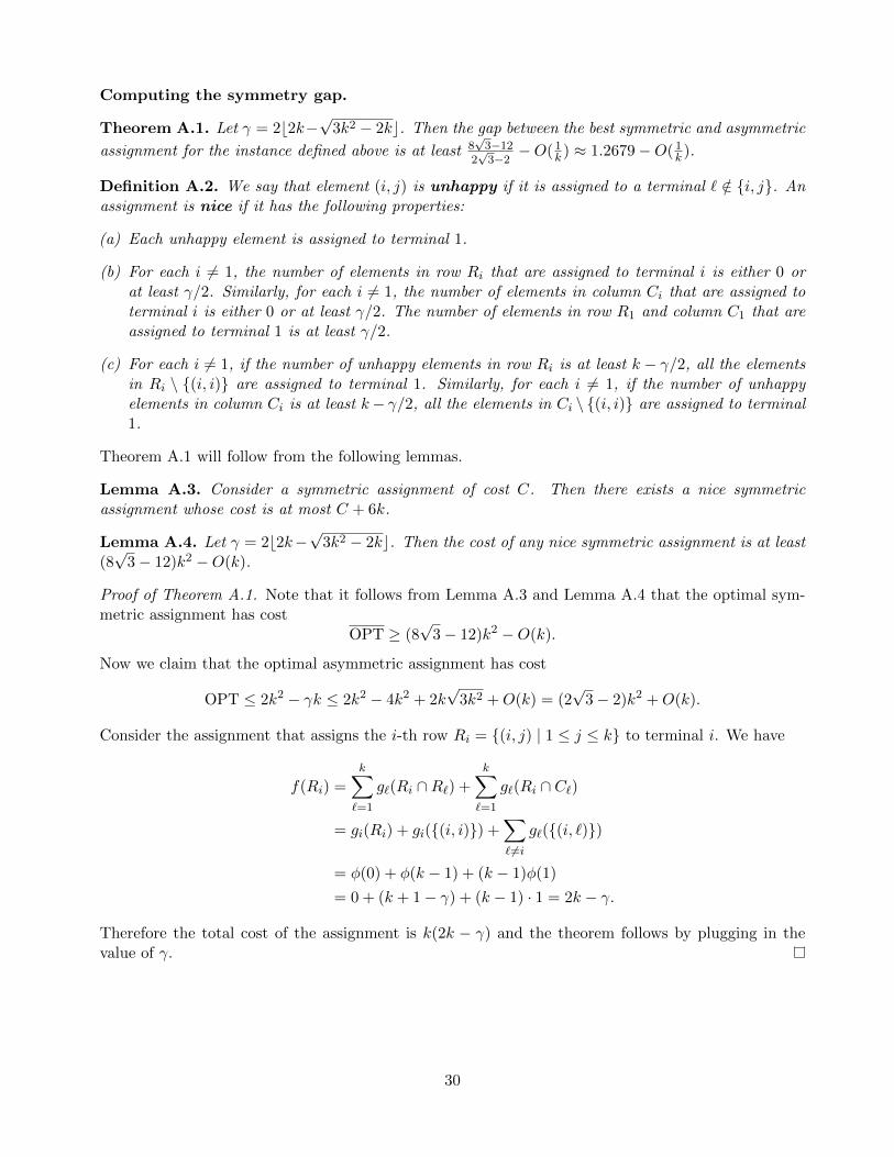
Computing the symmetry gap.

Theorem A.1. Let γ = 2b2k−√

3k2 − 2kc. Then the gap between the best symmetric and asymmetric

assignment for the instance defined above is at least 8√

3−122√

3−2−O( 1

k ) ≈ 1.2679−O( 1k ).

Definition A.2. We say that element (i, j) is unhappy if it is assigned to a terminal ` /∈ i, j. Anassignment is nice if it has the following properties:

(a) Each unhappy element is assigned to terminal 1.

(b) For each i 6= 1, the number of elements in row Ri that are assigned to terminal i is either 0 orat least γ/2. Similarly, for each i 6= 1, the number of elements in column Ci that are assigned toterminal i is either 0 or at least γ/2. The number of elements in row R1 and column C1 that areassigned to terminal 1 is at least γ/2.

(c) For each i 6= 1, if the number of unhappy elements in row Ri is at least k − γ/2, all the elementsin Ri \ (i, i) are assigned to terminal 1. Similarly, for each i 6= 1, if the number of unhappyelements in column Ci is at least k− γ/2, all the elements in Ci \ (i, i) are assigned to terminal1.

Theorem A.1 will follow from the following lemmas.

Lemma A.3. Consider a symmetric assignment of cost C. Then there exists a nice symmetricassignment whose cost is at most C + 6k.

Lemma A.4. Let γ = 2b2k−√

3k2 − 2kc. Then the cost of any nice symmetric assignment is at least(8√

3− 12)k2 −O(k).

Proof of Theorem A.1. Note that it follows from Lemma A.3 and Lemma A.4 that the optimal sym-metric assignment has cost

OPT ≥ (8√

3− 12)k2 −O(k).

Now we claim that the optimal asymmetric assignment has cost

OPT ≤ 2k2 − γk ≤ 2k2 − 4k2 + 2k√

3k2 +O(k) = (2√

3− 2)k2 +O(k).

Consider the assignment that assigns the i-th row Ri = (i, j) | 1 ≤ j ≤ k to terminal i. We have

f(Ri) =k∑`=1

g`(Ri ∩R`) +k∑`=1

g`(Ri ∩ C`)

= gi(Ri) + gi((i, i)) +∑` 6=i

g`((i, `))

= φ(0) + φ(k − 1) + (k − 1)φ(1)

= 0 + (k + 1− γ) + (k − 1) · 1 = 2k − γ.

Therefore the total cost of the assignment is k(2k − γ) and the theorem follows by plugging in thevalue of γ.

30

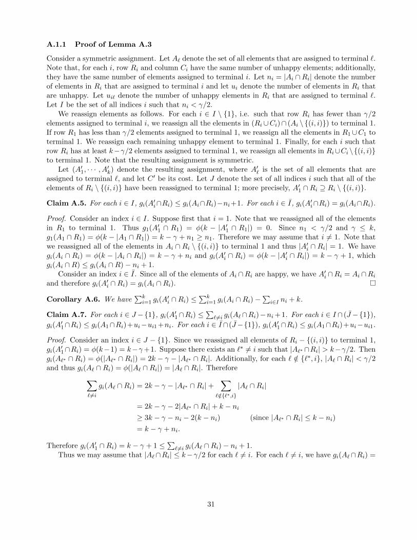
A.1.1 Proof of Lemma A.3

Consider a symmetric assignment. Let A` denote the set of all elements that are assigned to terminal `.Note that, for each i, row Ri and column Ci have the same number of unhappy elements; additionally,they have the same number of elements assigned to terminal i. Let ni = |Ai ∩Ri| denote the numberof elements in Ri that are assigned to terminal i and let ui denote the number of elements in Ri thatare unhappy. Let ui` denote the number of unhappy elements in Ri that are assigned to terminal `.Let I be the set of all indices i such that ni < γ/2.

We reassign elements as follows. For each i ∈ I \ 1, i.e. such that row Ri has fewer than γ/2elements assigned to terminal i, we reassign all the elements in (Ri ∪Ci)∩ (Ai \ (i, i)) to terminal 1.If row R1 has less than γ/2 elements assigned to terminal 1, we reassign all the elements in R1∪C1 toterminal 1. We reassign each remaining unhappy element to terminal 1. Finally, for each i such thatrow Ri has at least k−γ/2 elements assigned to terminal 1, we reassign all elements in Ri∪Ci \(i, i)to terminal 1. Note that the resulting assignment is symmetric.

Let (A′1, · · · , A′k) denote the resulting assignment, where A′` is the set of all elements that areassigned to terminal `, and let C ′ be its cost. Let J denote the set of all indices i such that all of theelements of Ri \ (i, i) have been reassigned to terminal 1; more precisely, A′1 ∩Ri ⊇ Ri \ (i, i).

Claim A.5. For each i ∈ I, gi(A′i∩Ri) ≤ gi(Ai∩Ri)−ni+1. For each i ∈ I, gi(A

′i∩Ri) = gi(Ai∩Ri).

Proof. Consider an index i ∈ I. Suppose first that i = 1. Note that we reassigned all of the elementsin R1 to terminal 1. Thus g1(A′1 ∩ R1) = φ(k − |A′1 ∩ R1|) = 0. Since n1 < γ/2 and γ ≤ k,g1(A1 ∩ R1) = φ(k − |A1 ∩ R1|) = k − γ + n1 ≥ n1. Therefore we may assume that i 6= 1. Note thatwe reassigned all of the elements in Ai ∩ Ri \ (i, i) to terminal 1 and thus |A′i ∩ Ri| = 1. We havegi(Ai ∩ Ri) = φ(k − |Ai ∩ Ri|) = k − γ + ni and gi(A

′i ∩ Ri) = φ(k − |A′i ∩ Ri|) = k − γ + 1, which

gi(Ai ∩R) ≤ gi(Ai ∩R)− ni + 1.Consider an index i ∈ I. Since all of the elements of Ai ∩Ri are happy, we have A′i ∩Ri = Ai ∩Ri

and therefore gi(A′i ∩Ri) = gi(Ai ∩Ri).

Corollary A.6. We have∑k

i=1 gi(A′i ∩Ri) ≤

∑ki=1 gi(Ai ∩Ri)−

∑i∈I ni + k.

Claim A.7. For each i ∈ J −1, gi(A′1∩Ri) ≤∑

`6=i gi(A`∩Ri)−ni+ 1. For each i ∈ I ∩ (J −1),gi(A

′1∩Ri) ≤ gi(A1∩Ri)+ui−ui1 +ni. For each i ∈ I∩(J−1), gi(A′1∩Ri) ≤ gi(A1∩Ri)+ui−ui1.

Proof. Consider an index i ∈ J − 1. Since we reassigned all elements of Ri − (i, i) to terminal 1,gi(A

′1∩Ri) = φ(k−1) = k−γ+1. Suppose there exists an `∗ 6= i such that |A`∗ ∩Ri| > k−γ/2. Then

gi(A`∗ ∩ Ri) = φ(|A`∗ ∩ Ri|) = 2k − γ − |A`∗ ∩ Ri|. Additionally, for each ` /∈ `∗, i, |A` ∩ Ri| < γ/2and thus gi(A` ∩Ri) = φ(|A` ∩Ri|) = |A` ∩Ri|. Therefore∑

6=igi(A` ∩Ri) = 2k − γ − |A`∗ ∩Ri|+

∑`/∈`∗,i

|A` ∩Ri|

= 2k − γ − 2|A`∗ ∩Ri|+ k − ni≥ 3k − γ − ni − 2(k − ni) (since |A`∗ ∩Ri| ≤ k − ni)= k − γ + ni.

Therefore gi(A′1 ∩Ri) = k − γ + 1 ≤

∑` 6=i gi(A` ∩Ri)− ni + 1.

Thus we may assume that |A`∩Ri| ≤ k−γ/2 for each ` 6= i. For each ` 6= i, we have gi(A`∩Ri) =

31

φ(|A` ∩Ri|) = |A` ∩Ri|. Thus∑6=igi(A` ∩Ri) = k − ni,

gi(A′1 ∩Ri) = k − γ + 1

=∑` 6=i

gi(A` ∩Ri) + ni − γ + 1

≤∑` 6=i

gi(A` ∩Ri)− ni + 1 (since γ ≥ 0).

Consider an index i ∈ I ∩ (J \ 1). Then ni < γ/2 and ui + ni < k − γ/2. The elements of Rithat we reassigned to terminal 1 were the unhappy elements and the elements of Ai ∩Ri. Note that,since i 6= 1, at most one element of A1 ∩ Ri is happy (namely the element (i, 1) ∈ C1). Therefore|A′1∩Ri| ≤ ui+ni+ 1 ≤ k−γ/2 and |A1∩Ri| ≤ ui1 + 1 ≤ k−γ/2. Thus gi(A

′1∩Ri) = φ(|A′1∩Ri|) =

|A′1 ∩Ri| = |A1 ∩Ri|+ ui − ui1 + ni and gi(A1 ∩Ri) = φ(|A1 ∩Ri|) = |A1 ∩Ri|.Consider an index i ∈ I ∩ (J \ 1). Then ni ≥ γ/2 and ui < k − γ/2. The elements of Ri that

we reassigned to terminal 1 were the unhappy elements. Note that at most one element of A1 ∩Ri ishappy and therefore |A′1 ∩Ri| ≤ ui + 1 ≤ k − γ/2. Additionally, |A1 ∩Ri| ≤ ui1 + 1 ≤ k − γ/2. Thusgi(A

′1∩Ri) = φ(|A′1∩Ri|) = |A′1∩Ri| = |A1∩Ri|+ui−ui1 and gi(A1∩Ri) = φ(|A1∩Ri|) = |A1∩Ri|.

Claim A.8. For each i ∈ J and each ` /∈ i, 1, gi(A′` ∩Ri) = 0. For each i ∈ J and each ` /∈ i, 1,gi(A

′` ∩Ri) ≤ gi(A` ∩Ri)− ui`.

Proof. Consider an index i ∈ J . Then Ri\(i, i) ⊆ A′1. It follows that, for each ` /∈ i, 1, A′`∩Ri = ∅and gi(A

′` ∩Ri) = φ(|A′` ∩Ri|) = 0.

Consider an index i ∈ J and an index ` /∈ i, 1. Since i ∈ J , we have ui < k − γ/2. Notethat at most one element of A` ∩ Ri is happy and thus |A` ∩ Ri| ≤ ui` + 1 ≤ k − γ/2. Moreover,|A′` ∩ Ri| = |A` ∩ Ri| − ui` ≤ 1. Thus gi(A` ∩ Ri) = φ(|A` ∩ Ri|) = |A` ∩ Ri| and gi(A

′` ∩ Ri) =

φ(|A′` ∩Ri|) = |A′` ∩Ri| = |A` ∩Ri| − ui`.

Corollary A.9. We have∑i∈J−1

∑6=igi(A

′` ∩Ri) ≤

∑i∈J−1

∑`6=i

gi(A` ∩Ri)−∑

i∈J−1

ni + k.

Proof. By the preceding claims, we have∑i∈J−1

gi(A′1 ∩Ri) ≤

∑i∈J−1

∑`6=i

gi(A` ∩Ri)−∑

i∈J−1

ni + k

∑i∈J−1

∑`/∈i,1

gi(A′` ∩Ri) = 0

∑i∈J−1

∑` 6=i

gi(A′` ∩Ri) =

∑i∈J−1

gi(A′1 ∩Ri) +

∑i∈J−1

∑`/∈i,1

gi(A′` ∩Ri)

≤∑

i∈J−1

∑`6=i

gi(A` ∩Ri)−∑

i∈J−1

ni + k.

32

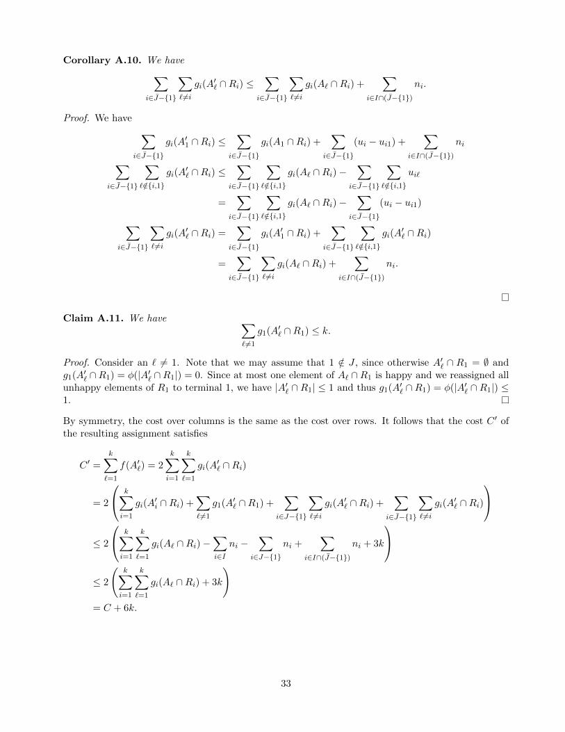
Corollary A.10. We have∑i∈J−1

∑` 6=i

gi(A′` ∩Ri) ≤

∑i∈J−1

∑`6=i

gi(A` ∩Ri) +∑

i∈I∩(J−1)

ni.

Proof. We have ∑i∈J−1

gi(A′1 ∩Ri) ≤

∑i∈J−1

gi(A1 ∩Ri) +∑

i∈J−1

(ui − ui1) +∑

i∈I∩(J−1)

ni

∑i∈J−1

∑`/∈i,1

gi(A′` ∩Ri) ≤

∑i∈J−1

∑`/∈i,1

gi(A` ∩Ri)−∑

i∈J−1

∑`/∈i,1

ui`

=∑

i∈J−1

∑`/∈i,1

gi(A` ∩Ri)−∑

i∈J−1

(ui − ui1)

∑i∈J−1

∑6=igi(A

′` ∩Ri) =

∑i∈J−1

gi(A′1 ∩Ri) +

∑i∈J−1

∑`/∈i,1

gi(A′` ∩Ri)

=∑

i∈J−1

∑`6=i

gi(A` ∩Ri) +∑

i∈I∩(J−1)

ni.

Claim A.11. We have ∑`6=1

g1(A′` ∩R1) ≤ k.

Proof. Consider an ` 6= 1. Note that we may assume that 1 /∈ J , since otherwise A′` ∩ R1 = ∅ andg1(A′` ∩R1) = φ(|A′` ∩R1|) = 0. Since at most one element of A` ∩R1 is happy and we reassigned allunhappy elements of R1 to terminal 1, we have |A′` ∩R1| ≤ 1 and thus g1(A′` ∩R1) = φ(|A′` ∩R1|) ≤1.

By symmetry, the cost over columns is the same as the cost over rows. It follows that the cost C ′ ofthe resulting assignment satisfies

C ′ =

k∑`=1

f(A′`) = 2

k∑i=1

k∑`=1

gi(A′` ∩Ri)

= 2

k∑i=1

gi(A′i ∩Ri) +

∑6=1

g1(A′` ∩R1) +∑

i∈J−1

∑`6=i

gi(A′` ∩Ri) +

∑i∈J−1

∑`6=i

gi(A′` ∩Ri)

≤ 2

k∑i=1

k∑`=1

gi(A` ∩Ri)−∑i∈I

ni −∑

i∈J−1

ni +∑

i∈I∩(J−1)

ni + 3k

≤ 2

(k∑i=1

k∑`=1

gi(A` ∩Ri) + 3k

)= C + 6k.

33

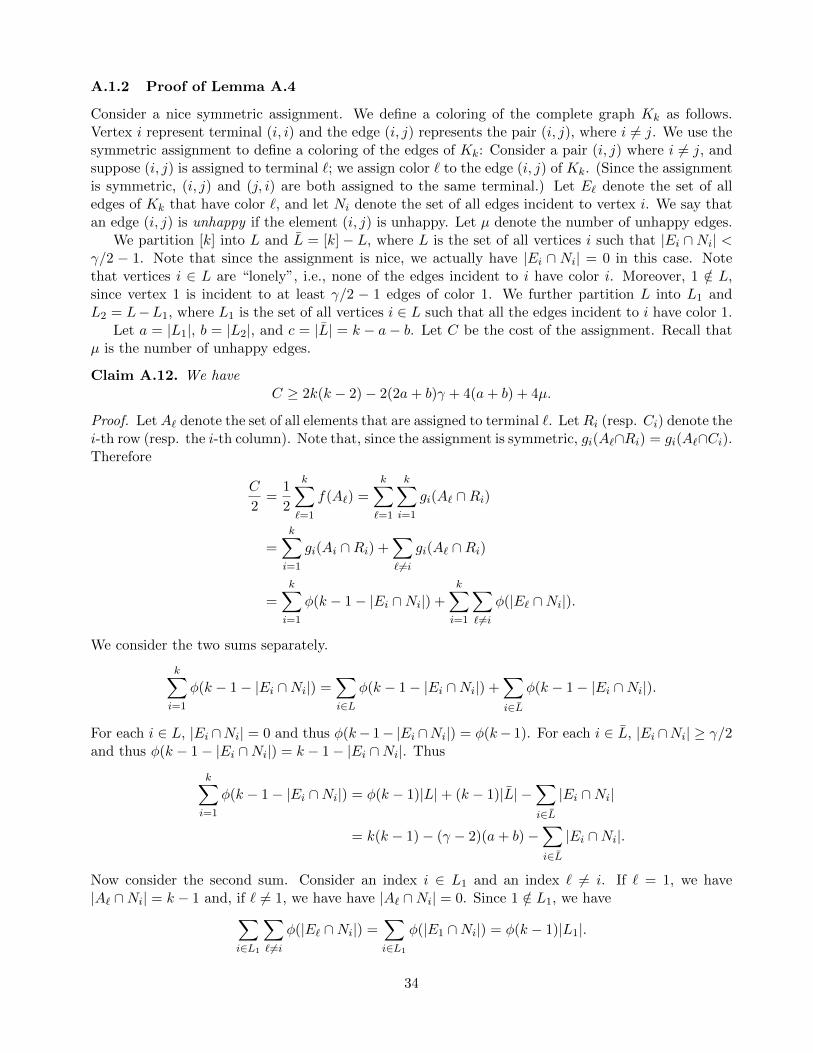
A.1.2 Proof of Lemma A.4

Consider a nice symmetric assignment. We define a coloring of the complete graph Kk as follows.Vertex i represent terminal (i, i) and the edge (i, j) represents the pair (i, j), where i 6= j. We use thesymmetric assignment to define a coloring of the edges of Kk: Consider a pair (i, j) where i 6= j, andsuppose (i, j) is assigned to terminal `; we assign color ` to the edge (i, j) of Kk. (Since the assignmentis symmetric, (i, j) and (j, i) are both assigned to the same terminal.) Let E` denote the set of alledges of Kk that have color `, and let Ni denote the set of all edges incident to vertex i. We say thatan edge (i, j) is unhappy if the element (i, j) is unhappy. Let µ denote the number of unhappy edges.

We partition [k] into L and L = [k]− L, where L is the set of all vertices i such that |Ei ∩Ni| <γ/2 − 1. Note that since the assignment is nice, we actually have |Ei ∩ Ni| = 0 in this case. Notethat vertices i ∈ L are “lonely”, i.e., none of the edges incident to i have color i. Moreover, 1 /∈ L,since vertex 1 is incident to at least γ/2 − 1 edges of color 1. We further partition L into L1 andL2 = L−L1, where L1 is the set of all vertices i ∈ L such that all the edges incident to i have color 1.

Let a = |L1|, b = |L2|, and c = |L| = k − a− b. Let C be the cost of the assignment. Recall thatµ is the number of unhappy edges.

Claim A.12. We haveC ≥ 2k(k − 2)− 2(2a+ b)γ + 4(a+ b) + 4µ.

Proof. Let A` denote the set of all elements that are assigned to terminal `. LetRi (resp. Ci) denote thei-th row (resp. the i-th column). Note that, since the assignment is symmetric, gi(A`∩Ri) = gi(A`∩Ci).Therefore

C

2=

1

2

k∑`=1

f(A`) =

k∑`=1

k∑i=1

gi(A` ∩Ri)

=

k∑i=1

gi(Ai ∩Ri) +∑` 6=i

gi(A` ∩Ri)

=

k∑i=1

φ(k − 1− |Ei ∩Ni|) +

k∑i=1

∑` 6=i

φ(|E` ∩Ni|).

We consider the two sums separately.

k∑i=1

φ(k − 1− |Ei ∩Ni|) =∑i∈L

φ(k − 1− |Ei ∩Ni|) +∑i∈L

φ(k − 1− |Ei ∩Ni|).

For each i ∈ L, |Ei ∩Ni| = 0 and thus φ(k− 1− |Ei ∩Ni|) = φ(k− 1). For each i ∈ L, |Ei ∩Ni| ≥ γ/2and thus φ(k − 1− |Ei ∩Ni|) = k − 1− |Ei ∩Ni|. Thus

k∑i=1

φ(k − 1− |Ei ∩Ni|) = φ(k − 1)|L|+ (k − 1)|L| −∑i∈L

|Ei ∩Ni|

= k(k − 1)− (γ − 2)(a+ b)−∑i∈L

|Ei ∩Ni|.

Now consider the second sum. Consider an index i ∈ L1 and an index ` 6= i. If ` = 1, we have|A` ∩Ni| = k − 1 and, if ` 6= 1, we have have |A` ∩Ni| = 0. Since 1 /∈ L1, we have∑

i∈L1

∑6=iφ(|E` ∩Ni|) =

∑i∈L1

φ(|E1 ∩Ni|) = φ(k − 1)|L1|.

34

Therefore we have

k∑i=1

∑6=iφ(|E` ∩Ni|) =

∑i∈L1

∑` 6=i

φ(|E` ∩Ni|) +∑i∈L2

∑`6=i

φ(|E` ∩Ni|) +∑i∈L

∑` 6=i

φ(|E` ∩Ni|)

= φ(k − 1)|L1|+∑i∈L2

∑` 6=i

φ(|E` ∩Ni|) +∑i∈L

∑`6=i|E` ∩Ni|

= (k + 1− γ)a+∑i∈L2

∑`6=i

φ(|E` ∩Ni|) +∑i∈L

∑`6=i|E` ∩Ni|.

Consider an index i ∈ L2 \ 1. If there exists an ` 6= i such that |E` ∩Ni| > k− γ/2, at least k− γ/2edges incident to i are unhappy and therefore all of the edges incident to i have color 1. But i has atleast γ/2 edges incident to it that have color i and therefore |E` ∩Ni| ≤ k − γ/2 for all ` 6= i. Thus,for each i ∈ L2 \ 1, we have ∑

6=iφ(|E` ∩Ni|) =

∑`6=i|E` ∩Ni|.

Thereforek∑i=1

∑` 6=i

φ(|E` ∩Ni|) ≥ (k + 1− γ)a− k +∑

i∈L2∪L

∑`6=i|E` ∩Ni|.

By combining the inequalities derived so far, it follows that

C

2≥ k(k − 1) + k(a− 1)− (2a+ b)γ + 3a+ 2b−

∑i∈L

|Ei ∩Ni|+∑

i∈L2∪L

∑`6=i|E` ∩Ni|.

Recall that, for each i ∈ L1, all of the edges incident to i have color one. Thus∑

i∈L1

∑`6=i |E`∩Ni| =∑

i∈L1|E1 ∩Ni| = (k − 1)a, and therefore

C

2≥ k(k − 2)− (2a+ b)γ + 2(a+ b)−

∑i∈L

|Ei ∩Ni|+k∑i=1

∑` 6=i|E` ∩Ni|.

In fact, the sum of L can be replaced by a sum over all i, because vertices in L do not have any edge ofcolor i incident to them. Each unhappy edge contributes 2 to the sum

∑ki=1

∑`6=i |E` ∩Ni|, and each

happy edge contributes 1 to the sum∑k

i=1

∑`6=i |E` ∩Ni|. Moreover, each unhappy edge contributes

0 to the sum∑k

i=1 |Ei ∩ Ni|, and each happy edge contributes 1 to the sum∑k

i=1 |Ei ∩ Ni|. Recallthat the number of unhappy edges is µ. Thus we have

k∑i=1

∑6=i|E` ∩Ni| −

∑i∈L

|Ei ∩Ni| =k∑i=1

∑`6=i|E` ∩Ni| −

k∑i=1

|Ei ∩Ni| = 2µ.

ThereforeC

2≥ k(k − 2)− (2a+ b)γ + 2(a+ b) + 2µ.

Claim A.13. The number of unhappy edges µ satisfies

µ ≥ (a+ b)(a+ b− 1)

2+ a(k − a− b− 1).

35

Proof. For each vertex i ∈ L, there are no edges incident to L that have color i. Therefore all edgeswith both endpoints in i are unhappy; there are (a + b)(a + b − 1)/2 such edges. Additionally, theedges incident to a vertex in L1 have color 1. Therefore all edges (i, j) such that i ∈ L1 and j ∈ L andj 6= 1 are also unhappy; there are at least a(c− 1) = a(k − a− b− 1) such edges.

Proof of Lemma A.4. It follows from the previous claims that the total cost C satisfies

C ≥ 2k(k − 2) + 2a(2k − 2γ − a− 2) + 2b(b− γ).

Let h(a, b) = 2k(k − 2) + 2a(2k − 2γ − a − 2) + 2b(b − γ). The function h(a, b) is concave in a andtherefore it is minimized when a = 0 or a = k.

Consider the case a = 0. By taking the derivative of h(0, b) with respect to b and setting it tozero, we see that h(0, b) is minimized when b = γ/2. Consider the case a = k. Since a + b ≤ k, wehave b = 0. Thus C ≥ minh(0, γ/2), h(k, 0). We choose γ = 2b2k −

√3k2 − 2kc which makes the

two expressions equal (up to the rounding of γ). This implies

C ≥ (8√

3− 12)k2 −O(k).

A.2 From oracle hardness to computational hardness

Here we explain how the hardness results in the value oracle model (the first parts of Theorem 3.1and 3.5) imply the analogous computational hardness results in these theorems. The key techniquehere is the use of list-decodable codes for the encoding of a “hidden partition”, as introduced in [8].The technique, although presented in [8] for submodular maximization problems, applies practicallywithout any change to submodular minimization as well. For concreteness, let us summarize how thistechnique applies to the Sub-MP problem:

We generate instances on a ground set X = N × V , where V = [k] × [k] is the ground set of ourinitial symmetric instance. The goal is to present an objective function f : 2X → R+ in a form thatmakes it difficult to distinguish the elements in sets N ×(i, j) from elements in N ×(j, i), for anyfixed i, j. More precisely, we construct a partition of N ×V into sets Aij : (i, j) ∈ [k]× [k] such thatit is hard to distinguish the elements in Aij from the elements in Aji.

We accomplish this by way of a list-decodable code as follows (the construction is simplified for thisparticular case): We consider a Unique-SAT instance φ with m variables, and an encoding function

E : 0, 1m → 0, 1N×(k2). The satisfying assignment x∗ of φ (if it exists) implicitly defines a partitionof N × [k]× [k] into subsets Aij : (i, j) ∈ [k]× [k], by specifying that for i < j,

Aij = (a, i, j) ∈ N × [k]× [k] : (E(x∗))a,i,j = 0 ∪ (a, j, i) ∈ N × [k]× [k] : (E(x∗))a,i,j = 1.

In other words, the string E(x∗) tells us which pairs of elements (a, i, j), (a, j, i) should be swapped,to obtain the sets Aij from the sets N × (i, j). In particular, if E(x∗) is the all-zeros string, thenAij = N × (i, j). For i = j, we define Aii = N × (i, i) in every case.

The encoding of an objective function for Sub-MP then consists purely of the Unique-SAT instanceφ, which is interpreted as follows. If φ is satisfiable, it induces the sets Aij as above, and the objective

function is understood to be f(S) = F (ξ), where ξij =|S∩Aij ||Aij | and F is the smooth submodular

function we described in Section 3. If φ is not satisfiable, then the objective function is understood tobe f(S) = G(ξ), with the same notation as in Section 3. We know that the gap between the optimain these two cases can be made arbitrarily close to 2− 2/k, and if we could distinguish the two cases,

36

we could determine whether a Unique-SAT instance has 0 or 1 satisfying assignments, which wouldimply NP = RP .

The question, however, is whether this is a legitimate encoding of the objective function, in thesense that given the encoding φ and a set S, the value of f(S) can be computed efficiently. The maininsight of [8] is that list-decodable codes allow us to evaluate such functions efficiently. The reason forthis is that the functions F (x), G(x) are constructed in such a way (going back to [24], see Lemma 3.2)that their value depends on the hidden partition Aij only if x is significantly unbalanced, meaning that∑

a∈Aijxa −

∑a∈Aji

xa > βn for some i, j ∈ [k] and constant β > 0. Equivalently, this means that to

evaluate f(S) and g(S), we need to determine the hidden partition only if |S ∩ Aij | − |S ∩ Aji| > βnfor some i, j ∈ [k]. Fortunately, there are known list-decodable codes that allow us to determine thesatisfying assignment x∗ and the induced partition Aij : i, j ∈ [k], given any such set S (because itcorresponds to a corrupted message which is relatively close to the codeword E(x∗)).

To summarize, for a given set S, we are either able to determine x∗ and the induced partitionAij : i, j ∈ [k], in which case we are obviously able to evaluate f(S) or g(S); or we conclude thatS does not satisfy |S ∩ Aij | − |S ∩ Aji| > βn for any i, j ∈ [k], and in this case we do not need to

know the partition Aij : i, j ∈ [k] because f(S) = g(S) and g does not depend on the partition ofAij ∪ Aji into Aij and Aji. This concludes the proof that we presented a legitimate encoding of theobjective function.

For further details on this technique to convert oracle hardness results into computational hardness,we refer the reader to [8].

37