local feature extraction and learning for computer … tutorial on local...local feature extraction...
TRANSCRIPT

Local Feature Extraction and Learning
for Computer Vision
Bin Fan, Chinese Academy of Sciences, China
Jiwen Lu, Tsinghua University, China
Pascal Fua, EPFL, Switzerland
CVPR’2017 Tutorials
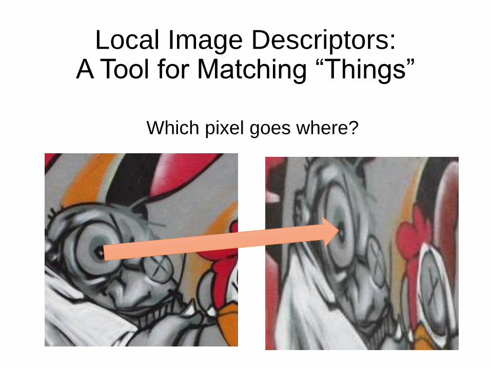
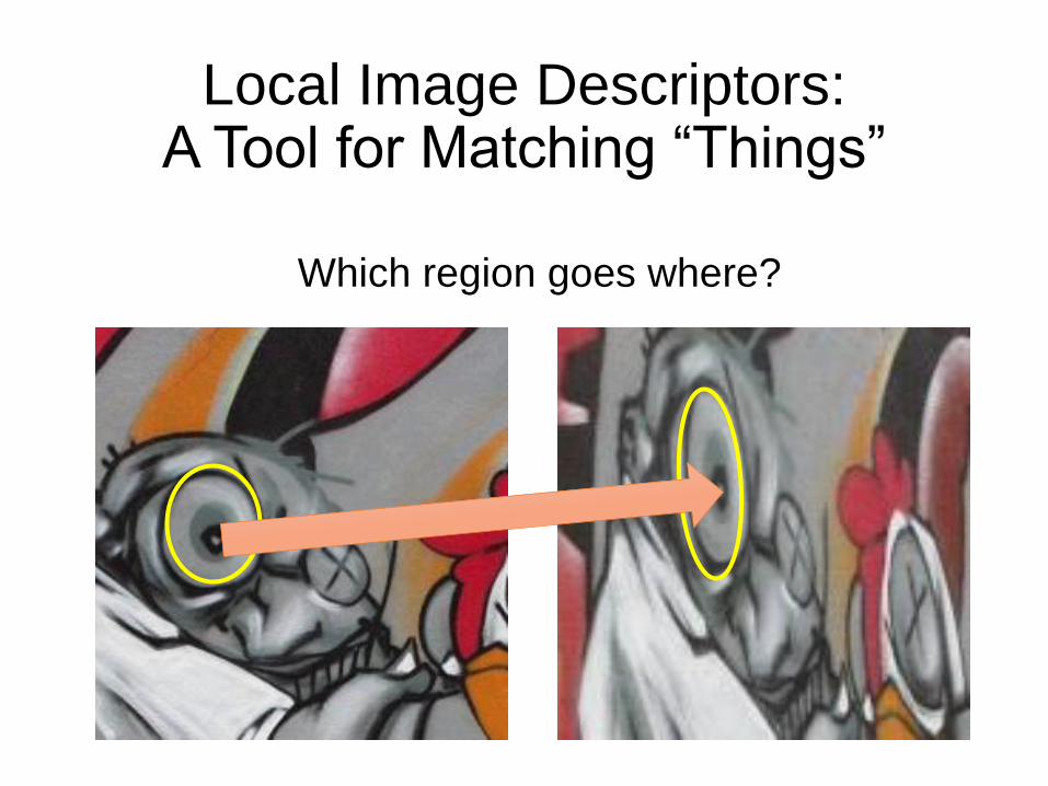
Local Image Descriptors: A Tool for Matching “Things”
Which pixel goes where?

Which region goes where?
Local Image Descriptors: A Tool for Matching “Things”

Dense city 3D reconstruction/ Structure from motion Content-based web image search
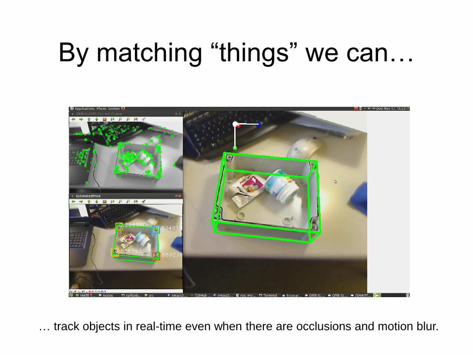
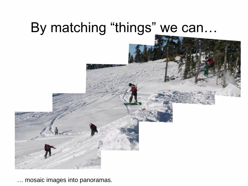
By matching “things” we can…
By matching “things” we can…
… track objects in real-time even when there are occlusions and motion blur.
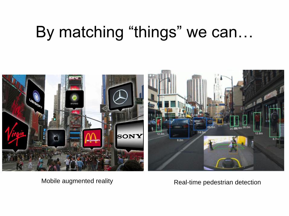
Mobile augmented reality Real-time pedestrian detection
By matching “things” we can…
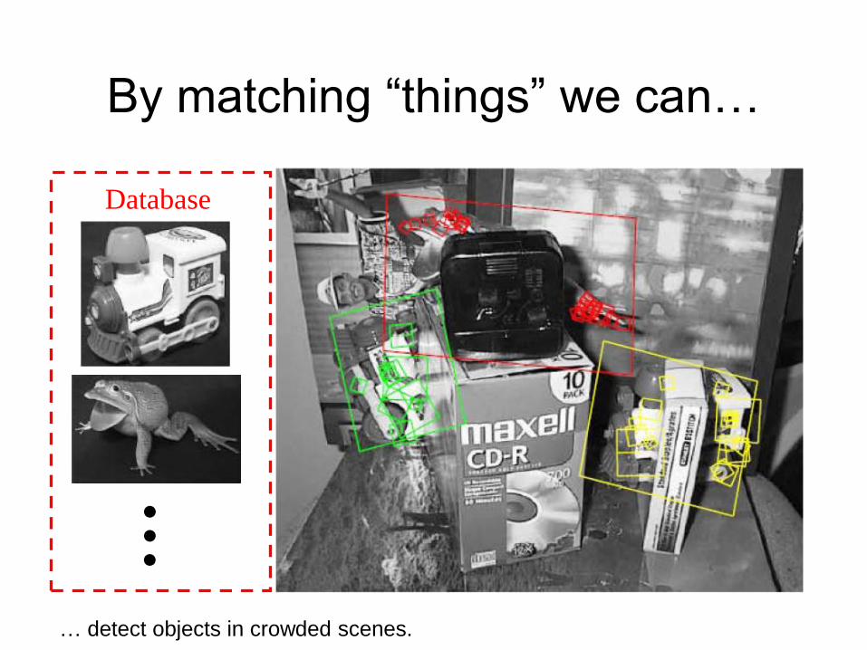
Database
…
By matching “things” we can…
… detect objects in crowded scenes.
By matching “things” we can…
… mosaic images into panoramas.
Which region goes where?
Local Image Descriptors: A Tool for Matching “Things”
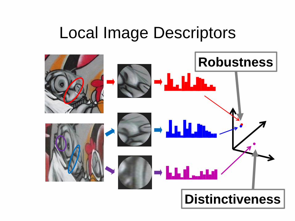
Distinctiveness
Robustness
Local Image Descriptors

SIFT and its variants
Early
methods
04 07 10 15
Learning based methods
CNN based methods
Binary descriptor
Local Descriptor Trends

Deep Learning Revolution
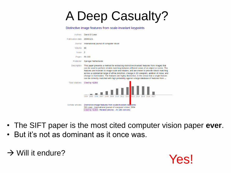
• The SIFT paper is the most cited computer vision paper ever.
• But it’s not as dominant as it once was.
Will it endure?
A Deep Casualty?
Yes!
Keypoints Remain Relevant
• When accurate geometric recovery matters, they remain
unequaled.
• They are efficient for real-time applications.
• They provide an effective way
• to compress the information present in large images,
• to recognize specific locations.
• The algorithms do not need to be retrained for each new
application.
• Some or all elements of the pipeline can deeply reformulated.
Future algorithms will combine Deep Learning and keypoint
matching.
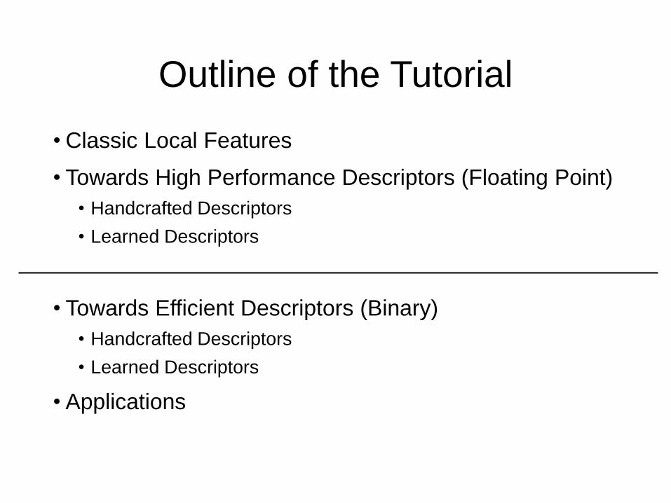
Outline of the Tutorial
• Classic Local Features
• Towards High Performance Descriptors (Floating Point)
• Handcrafted Descriptors
• Learned Descriptors
• Towards Efficient Descriptors (Binary)
• Handcrafted Descriptors
• Learned Descriptors
• Applications

Outline of the Tutorial
• Classic Local Features
• Towards High Performance Descriptors (Floating Point)
• Handcrafted Descriptors
• Learned Descriptors
• Towards Efficient Descriptors (Binary)
• Handcrafted Descriptors
• Learned Descriptors
• Applications

Classic Local Features
•SIFT: Scale Invariant Feature Transform
•SURF: Speeded Up Robust Features
•Daisy
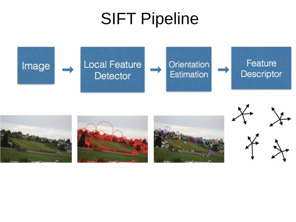
SIFT Pipeline

GSS: Gaussian Scale
Space is produced by
iteratively convolving the
last layer image with a
Gaussian kernel.
DoGSS: DoG Scale Space
is produced by subtracting
neighboring GSS layers.
Scale space detection
* By Cmglee - Own work, CC BY-SA 3.0, https://commons.wikimedia.org/w/index.php?curid=42549151
SIFT [Lowe’99] Classic Local Features
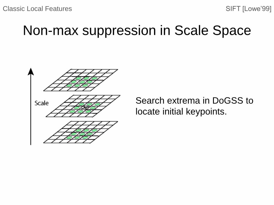
Search extrema in DoGSS to
locate initial keypoints.
Non-max suppression in Scale Space
SIFT [Lowe’99] Classic Local Features
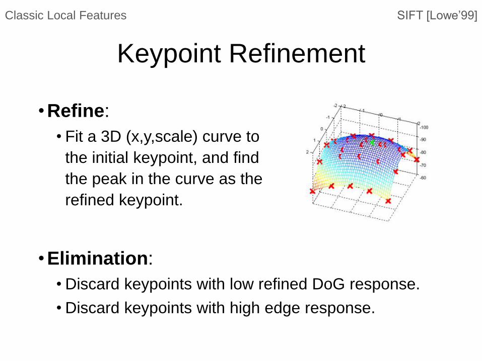
•Refine:
• Fit a 3D (x,y,scale) curve to
the initial keypoint, and find
the peak in the curve as the
refined keypoint.
•Elimination:
• Discard keypoints with low refined DoG response.
• Discard keypoints with high edge response.
Keypoint Refinement
SIFT [Lowe’99] Classic Local Features
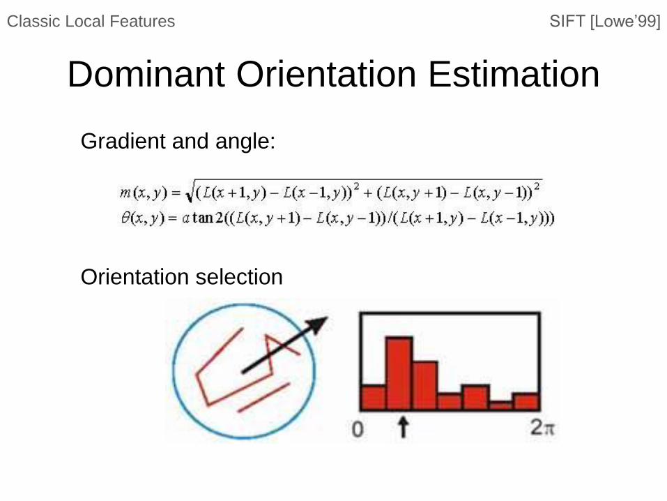
Gradient and angle:
Orientation selection
SIFT [Lowe’99] Classic Local Features
Dominant Orientation Estimation

SIFT [Lowe’99] Classic Local Features
Descriptor construction

SIFT [Lowe’99] Classic Local Features
Descriptor construction
1. Find the blurred image of the closest scale in scale space
2. Sample the points around the keypoint
3. Rotate the gradients and coordinates by dominant orientation
4. Separate the region into subregions
5. Create histogram for each sub region with 8 bins
6. Normalization

SURF [Bay ’04] Classic Local Features
Speeded Up Robust Features
•Aim: faster than SIFT, while still being robust.
• 3-7 times faster than SIFT, with similar matching
performance.
•Key Idea: Haar filters and Integral Image
•Well received!
• More than 8000 citations.
• CVIU Most Cited Paper
• Koenderink Prize of ECCV’16
• fundamental contributions in computer vision that stood the test of time
SURF [Bay ’04] Classic Local Features
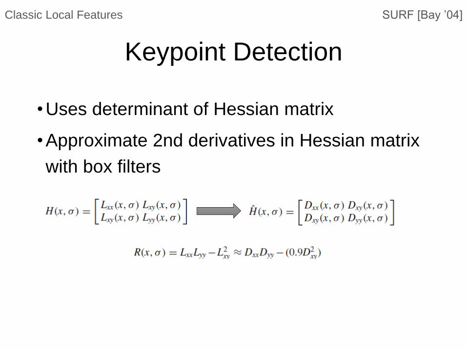
Keypoint Detection
•Uses determinant of Hessian matrix
•Approximate 2nd derivatives in Hessian matrix
with box filters

Lxx Lyy Lxy
Dxx Dyy Dxy
SURF [Bay ’04] Classic Local Features
Keypoint Detection
SURF SIFT
SURF [Bay ’04] Classic Local Features
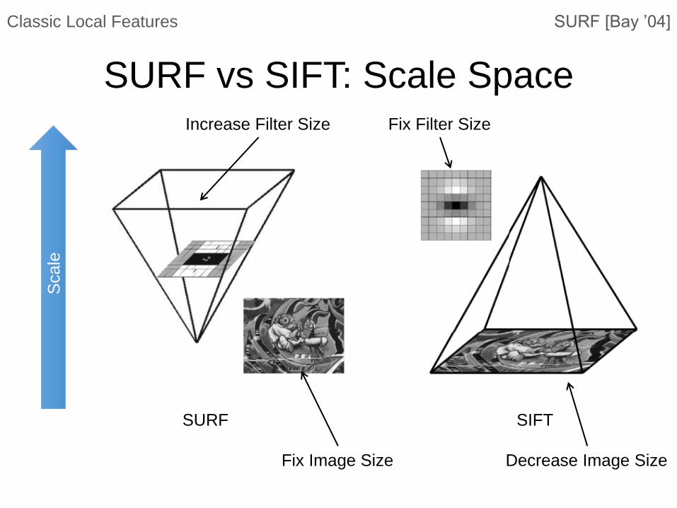
SURF vs SIFT: Scale Space S
cale
Fix Image Size
Increase Filter Size Fix Filter Size
Decrease Image Size
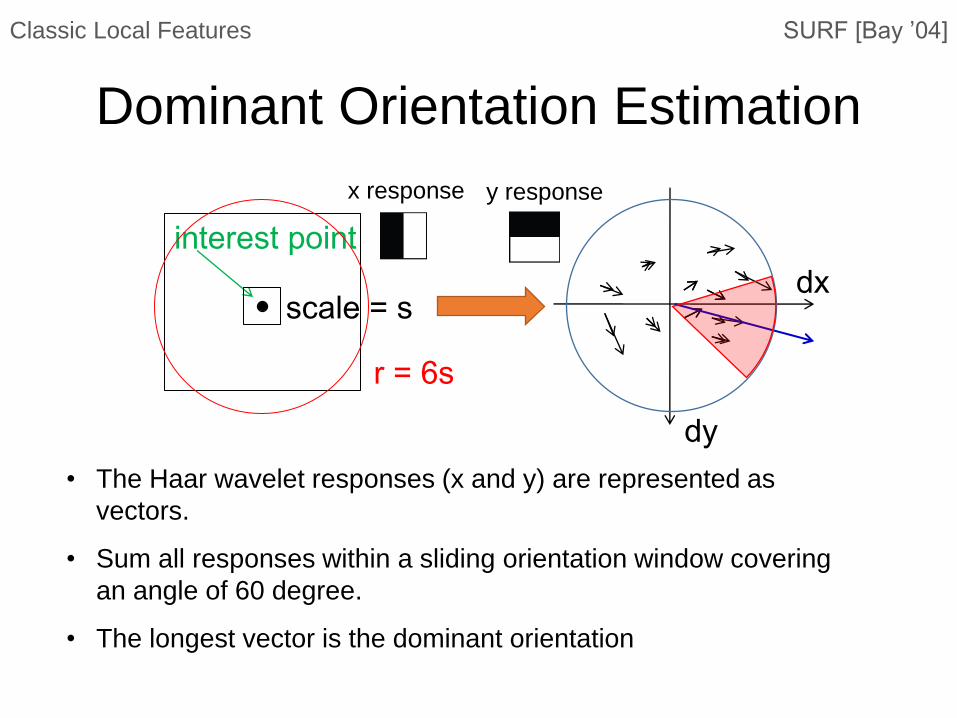
interest point
scale = s
r = 6s
dx
dy
x response y response
SURF [Bay ’04] Classic Local Features
Dominant Orientation Estimation
• The Haar wavelet responses (x and y) are represented as
vectors.
• Sum all responses within a sliding orientation window covering
an angle of 60 degree.
• The longest vector is the dominant orientation
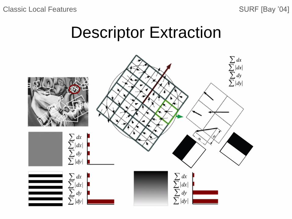
SURF [Bay ’04] Classic Local Features
Descriptor Extraction

1. Split the interest region (20s x 20s) into 4 x 4 square sub-regions.
2. Calculate Haar wavelet responses dx and dy, and weight the
responses with a Gaussian kernel.
3. Sum the response over each sub-region for dx and dy, then sum
the absolute value of response.
4. Concatenate summation
results in all sub-regions,
forming a 64D SURF
descriptor.
SURF [Bay ’04] Classic Local Features
Descriptor Extraction

Daisy [Tola ’08] Classic Local Features
DAISY Descriptor
• Log-polar grid arrangement
• Gaussian pooling of histograms of gradient orientations
• Efficient for dense computation, but not for sparse keypoints!

Daisy [Tola ’08] Classic Local Features
Efficient Dense Computation of Features
• The computation mostly involves 1D convolutions.
• Rotating the descriptor only involves reordering the histograms.