local fourier analysis for mixed ﬁnite-element methods for...

Local Fourier analysis for mixed finite-element methods for theStokes equations

Yunhui Hea,∗, Scott P. MacLachlana

aDepartment of Mathematics and Statistics, Memorial University of Newfoundland, St. John’s, NL A1C 5S7, Canada

Abstract

In this paper, we develop a local Fourier analysis of multigrid methods based on block-structuredrelaxation schemes for stable and stabilized mixed finite-element discretizations of the Stokesequations, to analyze their convergence behavior. Three relaxation schemes are considered: dis-tributive, Braess-Sarazin, and Uzawa relaxation. From this analysis, parameters that minimizethe local Fourier analysis smoothing factor are proposed for the stabilized methods with dis-tributive and Braess-Sarazin relaxation. Considering the failure of the local Fourier analysissmoothing factor in predicting the true two-grid convergence factor for the stable discretization,we numerically optimize the two-grid convergence predicted by local Fourier analysis in thiscase. We also compare the efficiency of the presented algorithms with variants using inexactsolvers. Finally, some numerical experiments are presented to validate the two-grid and multi-grid convergence factors.

Keywords: Monolithic multigrid, Block-structured relaxation, local Fourier analysis, mixedfinite-element methods, Stokes Equations2000 MSC: 65N55, 65F10, 65F08, 76M10

1. Introduction

In recent years, substantial research has been devoted to efficient numerical solution of theStokes and Navier-Stokes equations, due both to their utility as models of (viscous) fluids andtheir commonalities with many other physical problems that lead to saddle-point systems (see,for example [1], and many of the other references cited here). In the linear (or linearized) case,solution of the resulting matrix equations is seen to be difficult, due to indefiniteness and theusual ill-conditioning of discretized PDEs. In the literature, block preconditioners (cf. [1] andthe references therein) are widely used, due to their easy construction from standard multigrid al-gorithms for scalar elliptic PDEs, such as algebraic multigrid [2]. However, monolithic multigridapproaches [3, 4, 5, 6, 7] have been shown to outperform these preconditioners when algorithmicparameters are properly chosen [8, 9]. The focus of this work is on the analysis of such mono-lithic multigrid methods in the case of stable and stabilized finite-element discretizations of theStokes equations.

∗Corresponding author: Yunhui He. E-mail address: [email protected] addresses: [email protected] (Yunhui He), [email protected] (Scott P. MacLachlan)

Preprint submitted to Elsevier November 26, 2018

Local Fourier analysis (LFA) [10, 11] has been widely used to predict the convergence behav-ior of multigrid methods, to help design relaxation schemes and choose algorithmic parameters.In general, the LFA smoothing factor provides a sharp prediction of actual multigrid convergence,see [10], under the assumption of an “ideal” coarse-grid correction scheme (CGC) that annihi-lates low-frequency error components and leaves high-frequency components unchanged. Inpractice, the LFA smoothing and two-grid convergence factors often exactly match the true con-vergence factor of multigrid applied to a problem with periodic boundary conditions [12, 13, 10].Recently, the validity of LFA has been further analysed [14], extending this exact prediction toa wider class of problems. However, the LFA smoothing factor is also known to lose its predic-tivity of the true convergence in some cases [15, 16, 17]. In particular, the smoothing factor ofLFA overestimates the two-grid convergence factor for the Taylor-Hood (Q2 −Q1) discretizationof the Stokes equations with Vanka relaxation [16]. Even for the scalar Laplace operator, theLFA smoothing factor fails to predict the observed multigrid convergence factor for higher-orderfinite-element methods [15].

Two main questions interest us here. First, we look to extend the study of [16] to considerLFA of block-structured relaxation schemes for finite-element discretizations of the Stokes equa-tions. Secondly, we consider if the LFA smoothing factor can predict the convergence factorsfor these relaxation schemes. Recently, LFA for multigrid based on block-structured relaxationschemes applied to the marker-and-cell (MAC) finite-difference discretization of the Stokes equa-tions was shown to give a good prediction of convergence [18], in contrast to the results of [16].Thus, a natural question to investigate is whether the contrasting results between [18] and [16]is due to the differences in discretization or those in the relaxation schemes considered. Here,we apply the relaxation schemes of [18] to the Q2 − Q1 discretization from [16], as well as an“intermediate” discretization using stabilized Q1 − Q1 approaches.

In recent decades, many block relaxation schemes have been studied and applied to manyproblems, including Braess-Sarazin-type relaxation schemes [3, 19, 20, 4, 21], Vanka-type re-laxation schemes [3, 22, 4, 16, 23, 24, 7], Uzawa-type relaxation schemes [25, 26, 27, 6, 28], dis-tributive relaxation schemes [29, 5, 30, 31, 32] and other types of methods [33, 34]. Even thoughLFA has been applied to distributive relaxation [35, 11], Vanka relaxation [16, 24, 36, 37], andUzawa-type schemes [26] for the Stokes equations, most of the existing LFA has been for relax-ation schemes using (symmetric) Gauss-Seidel (GS) approaches, and for simple finite-differenceand finite-element discretizations. Considering modern multicore and accelerated parallel ar-chitectures, we focus on schemes based on weighted Jacobi relaxation with distributive, Braess-Sarazin, and Uzawa relaxation for common finite-element discretizations of the Stokes equations.

Some key conclusions of this analysis are as follows. First, while the LFA smoothing factorgives a good prediction of the true convergence factor for the stabilized discretizations with dis-tributive weighted Jacobi and Braess-Sarazin relaxation, it does not for the Uzawa relaxation (incontrast to what is seen for the MAC discretization [18, 35]). For no cases does the LFA smooth-ing factor offer a good prediction of the true convergence behaviour for the (stable) Q2 − Q1discretization, suggesting that the discretization is responsible for the lack of predictivity, con-sistent with the results in [15, 16]. For both stable and stabilized discretizations, we see thatstandard distributive weighted Jacobi relaxation loses some of its high efficiency, in contrast towhat is seen for the MAC scheme [18, 35] but that robustness can be restored with an additionalrelaxation sweep. Exact Braess-Sarazin relaxation is also highly effective, with LFA-predictedW(1, 1) convergence factors of 1

9 in the stabilized cases and 14 in the stable case. To realize these

rates with inexact cycles, however, requires nested W-cycles to solve the approximate Schurcomplement equation accurately enough in the stabilized case, although simple weighted Ja-

2

cobi on the approximate Schur complement is observed to be sufficient in the stable case. ForUzawa-type relaxation, we see a notable gap between predicted convergence with exact inver-sion of the resulting Schur complement, versus inexact inversion, although some improvementis seen when replacing the approximate Schur complement with a mass matrix approximation,as is commonly used in block-diagonal preconditioners [38, 39, 40]. Overall, however, we seethat distributive weighted Jacobi (DWJ) (with 2 sweeps of Jacobi relaxation on the pressureequation) outperforms both Braess-Sarazin relaxation (BSR) and Uzawa relaxation, for the sta-bilized discretizations, while DWJ and inexact BSR offer comparable performance for the stablediscretization.

We organize this paper as follows. In Section 2, we introduce two stabilized Q1 −Q1 and thestable Q2 − Q1 mixed finite-element discretizations of the Stokes equations in two dimensions(2D). In Section 3, we first review the LFA approach, then discuss the Fourier representation forthese discretizations. In Section 4, LFA is developed for DWJ, BSR, and Uzawa-type relaxation,and optimal LFA smoothing factors are derived for the two stabilized Q1 − Q1 methods withDWJ and BSR. Multigrid performance is presented to validate the theoretical results. Section5 exhibits optimized LFA two-grid convergence factors and measured multigrid convergencefactors for the Q2 − Q1 discretization. Furthermore, a comparison of the cost and effectivenessof the relaxation schemes is given. Conclusions are presented in Section 6.

2. Discretizations

In this paper, we consider the Stokes equations,

−∆~u + ∇p = ~f , (1)∇ · ~u = 0,

where ~u is the velocity vector, p is the (scalar) pressure of a viscous fluid, and ~f representsa (known) forcing term, together with suitable boundary conditions. Because of the nature ofLFA, we validate our predictions against the problem with periodic boundary conditions on both~u and p. Discretizations of (1) typically lead to a linear system of the following form:

Kx =

(A BT

B −βC

) (U

p

)=

(f0

)= b, (2)

where A corresponds to the discretized vector Laplacian, and B is the negative of the discretedivergence operator. If the discretization is naturally unstable, then C , 0 is the stabilizationmatrix, otherwise C = 0. In this paper, we discuss two stabilized Q1 −Q1 and the stable Q2 −Q1finite-element discretizations.

The natural finite-element approximation of Problem (1) is: Find ~uh ∈ Xh and ph ∈ H

h suchthat

a(~uh,~vh) + b(ph,~vh) + b(qh, ~uh) = g(~vh), for all~vh ∈ Xh0 and qh ∈ H

h, (3)

where

a(~uh,~vh) =

∫Ω

∇~uh : ∇~vh, b(ph,~vh) = −

∫Ω

ph∇ · ~vh,

g(~vh) =

∫Ω

~fh · ~vh,

3

and Xh ⊂ H1(Ω), Hh ⊂ L2(Ω) are finite-element spaces. Here, Xh0 ⊂ X

h satisfies homogeneousDirichlet boundary conditions in place of any non-homogenous essential boundary conditions onXh. Problem (3) has a unique solution only when Xh and Hh satisfy an inf-sup condition (see[1, 41, 42, 43]).

2.1. Stabilized Q1 − Q1 discretizations

The standard equal-order approximation of (3) is well-known to be unstable [42, 1]. Tocircumvent this, a scaled pressure Laplacian term can be added to (3); for a uniform mesh withsquare elements of size h, we subtract

c(ph, qh) = βh2(∇ph,∇qh),

for β > 0. With this, the resulting linear system is given by(A BT

B −βh2Ap

) (U

p

)=

(f0

)= b,

where Ap is the Q1 Laplacian operator for the pressure. Denote S = BA−1BT , and S β = BA−1BT +

βC, where C = h2Ap. From [1], the red-black unstable mode p = ±1, can be moved from a zeroeigenvalue to a unit eigenvalue ( giving stability without loss of accuracy) by choosing β so that

pT S βppT Qp

= βpT CppT Qp

= 1, (4)

where Q is the mass matrix. Substituting the bilinear stiffness and mass matrices into (4), wefind β = 1

24 . We refer to this method as the Poisson-stabilized discretization (PoSD).An L2 projection to stabilize the Q1 − Q1 discretization, proposed in [43], stabilizes with

C(ph, qh) = (ph − Π0 ph, qh − Π0qh), (5)

where Π0 is the L2 projection from Hh into the space of piecewise constant functions on themesh. We refer to this method as the projection stabilized discretization (PrSD). The 4 × 4element matrix C4 of (5) is given by

C4 = Q4 − qqT h2,

where Q4 is the 4×4 element mass matrix for the bilinear discretization and q =[

14

14

14

14

]T.

In the projection stabilized method, we can write C = Q − h2P, where P is given by the 9-pointstencil

P =14

14

12

14

12 1 1

214

12

14

.Applying (4) to C = Q − h2P, we find that β = 1 is the optimal choice.

4

2.2. Stable Q2 − Q1 discretizations

In order to guarantee the well-posedness of the discrete system (2) with C = 0, the discretiza-tion of the velocity and pressure unknowns should satisfy an inf-sup condition,

infqh,0

sup~vh,~0

|b(qh,~vh)|‖~vh‖1‖qh‖0

≥ Γ > 0,

where Γ is a constant. Taylor-Hood (Q2 − Q1) elements are well known to be stable [41, 1],where the basis functions associated with these elements are biquadratic for each component ofthe velocity field and bilinear for the pressure.

3. LFA preliminaries

3.1. Definitions and notations

In many cases, the LFA smoothing factor offers a good prediction of multigrid performance.Thus, we will explore the LFA smoothing factor and true (measured) multigrid convergence forthe three types of relaxations considered here. We first introduce some terminology of LFA,following [10, 11]. We consider the following two-dimensional infinite uniform grids,

G jh =

x j := (x j

1, xj2) = (k1, k2)h + δ j, (k1, k2) ∈ Z2,

with

δ j =

(0, 0) if j = 1,(0, h/2) if j = 2,(h/2, 0) if j = 3,(h/2, h/2) if j = 4.

The coarse grids, G j2h, are defined similarly.

Figure 1: At left, the mesh used for Q1 discretization. At right, the mesh used for Q2 discretization. Points marked by correspond to G1

h, those marked by 3 correspond to G2h, those marked by 2 correspond to G3

h and those marked by9correspond to G4

h.

5

Let Lh be a scalar Toeplitz operator defined by its stencil acting on G jh as follows:

Lh∧= [sκ]h (κ = (κ1, κ2) ∈ V); Lhwh(x j) =

∑κ∈V

sκwh(x j + κh), (6)

with constant coefficients sκ ∈ R (or C), where wh(x j) is a function in l2(G jh). Here, V ⊂ Z2 is a

finite index set. Because Lh is formally diagonalized by the Fourier modes ϕ(θ, x j) = eiθ·x j/h =

eiθ1 x j1/heiθ2 x j

2/h, where θ = (θ1, θ2) and i2 = −1, we use ϕ(θ, x j) as a Fourier basis with θ ∈[− π

2 ,3π2)2. High and low frequencies for standard coarsening (as considered here) are given by

θ ∈ T low =

[−π

2,π

2

)2, θ ∈ T high =

[−π

2,

3π2

)2 ∖ [−π

2,π

2

)2.

Definition 3.1. If, for all functions ϕ(θ, x j),

Lhϕ(θ, x j) = Lh(θ)ϕ(θ, x j),

we call Lh(θ) =∑κ∈V

sκeiθκ the symbol of Lh.

In what follows, we consider (3 × 3) linear systems of operators, which read

Lh =

L1,1

h L1,2h L1,3

hL2,1

h L2,2h L2,3

hL3,1

h L3,2h L3,3

h

=

−∆h 0 (∂x)h

0 −∆h (∂y)h

−(∂x)h −(∂y)h L3,3h

, (7)

where L3,3h depends on which discretization we use.

For the stabilized Q1 − Q1 approximations, the degrees of freedom for both velocity andpressure are only located on G1

h as pictured at left of Figure 1. In this setting, the Lk,`h (k, ` =

1, 2, 3) in (7) are scalar Toeplitz operators. Denote Lh as the symbol of Lh. Each entry in Lh

is computed as the (scalar) symbol of the corresponding block of Lk,`h , following Definition 3.1.

Thus, Lh is a 3 × 3 matrix. All blocks in Lh are diagonalized by the same transformation on acollocated mesh.

However, for the Q2 − Q1 discretization, the degrees of freedom for velocity are locatedon Gh =

⋃4j=1 G j

h, containing four types of meshpoints as shown at right of Figure 1. TheLaplace operator in (7) is defined by extending (6), with V taken to be a finite index set ofvalues, V = VN

⋃VX

⋃VY

⋃VC with VN ⊂ Z2, VX ⊂

(zx + 1

2 , zy)|(zx, zy) ∈ Z2, VY ⊂(zx, zy +

12 )|(zx, zy) ∈ Z2, and VC ⊂

(zx + 1

2 , zy + 12 )|(zx, zy) ∈ Z2

. With this, the (scalar) Q2 Laplace

operator is naturally treated as a block operator, and the Fourier representation of each blockcan be calculated based on Definition 3.1, with the Fourier bases adapted to account for thestaggering of the mesh points. Thus, the symbols of L1,1

h and L2,2h are 4 × 4 matrices. For more

details of LFA for the Laplace operator using higher-order finite-element methods, refer to [15].Similarly to the Laplace operator, both terms in the gradient, (∂x)h and (∂y)h, can be treated as(4×1)-block operators. Then, the symbols of L1,3

h and L2,3h are 4×1 matrices, calculated based on

Definition 3.1 adapted for the mesh staggering. The symbols of L3,1h and L3,2

h are the conjugatetransposes of those of L1,3

h and L2,3h , respectively. Finally, L3,3

h = 0. Accordingly, Lh is a 9 × 9matrix for the Q2 − Q1 discretization.

6

Definition 3.2. The error-propagation symbol, Sh(θ), for a block smoother Sh on the infinitegrid Gh satisfies

Shϕ(θ, x) = Shϕ(θ, x), θ ∈[−π

2,

3π2

)2,

for all ϕ(θ, x), and the corresponding smoothing factor for Sh is given by

µloc = µloc(Sh) = maxθ∈T high

∣∣∣λ(Sh(θ))∣∣∣ ,

where λ is an eigenvalue of Sh(θ).

In Definition 3.2, Gh = G1h for the stabilized case (and Sh(θ) is a 3 × 3 matrix) and Gh =⋃4

j=1 G jh for the stable case (where Sh(θ) is a 9 × 9 matrix).

The error-propagation symbol for a relaxation scheme, represented by matrix Mh, applied toeither the stabilized or stable scheme is written as

Sh(p, ω, θ) = I − ωM−1h (θ)Lh(θ),

where p represents parameters within Mh, the block approximation toLh, ω is an overall weight-ing factor, and Mh and Lh are the symbols for Mh andLh, respectively. Note that µloc is a functionof some parameters in Definition 3.2. In this paper, we focus on minimizing µloc with respect tothese parameters, to obtain the optimal LFA smoothing factor.

Definition 3.3. LetD be the set of allowable parameters and define the optimal smoothing factoroverD as

µopt = minD

µloc.

If the standard LFA assumption of an “ideal” CGC holds, then the two-grid convergencefactor can be estimated by the smoothing factor, which is easy to compute. However, as expected,we will see that this idealized CGC does not lead to a good prediction for some cases we considerbelow. When the LFA smoothing factor fails to predict the true two-grid convergence factor, theLFA two-grid convergence factor can still be used. Thus, we give a brief introduction to the LFAtwo-grid convergence factor in the following.

Let

α = (α1, α2) ∈(0, 0), (1, 0), (0, 1), (1, 1)

,

θα = (θα11 , θ

α22 ) = θ + π · α, θ := θ00 ∈ T low.

We use the ordering of α = (0, 0), (1, 0), (0, 1), (1, 1) for the four harmonics. To apply LFA to thetwo-grid operator,

MTGMh = S

ν2h M

CGCh S

ν1h , (8)

we require the representation of the CGC operator,

MCGCh = I − Ph(L∗2h)−1RhLh,

where Ph is the multigrid interpolation operator and Rh is the restriction operator. The coarse-gridoperator, L∗2h, can be either the Galerkin or rediscretization operator.

7

Inserting the representations of Sh,Lh,L∗2h, Ph,Rh into (8), we obtain the Fourier representa-

tion of two-grid error-propagation operator as

MTGMh (θ) = S

ν2

h (θ)(I − Ph(θ)(L∗2h(2θ))−1Rh(θ)Lh(θ)

)Sν1

h (θ),

where

Lh(θ) = diagLh(θ00), Lh(θ10), Lh(θ01), Lh(θ11)

,

Sh(θ) = diagSh(θ00), Sh(θ10), Sh(θ01), Sh(θ11)

,

Ph(θ) =(Ph(θ00); Ph(θ10); Ph(θ01); Ph(θ11)

),

Rh(θ) =(Rh(θ00), Rh(θ10), Rh(θ01), Rh(θ11)

),

in which diagT1,T2,T3,T4 stands for the block diagonal matrix with diagonal blocks, T1,T2,T3,and T4.

Here, we use the standard finite-element interpolation operators and their transposes for re-striction. For Q1, the symbol is well-known [10] while, for the nodal basis for Q2, the symbol isgiven in [15].

Definition 3.4. The asymptotic two-grid convergence factor, ρasp, is defined as

ρasp = supρ(Mh(θ)TGM) : θ ∈ T low.

In what follows, we consider a discrete form of ρasp, denoted by ρh, resulting from samplingρasp over only a finite set of frequencies. For simplicity, we drop the subscript h throughout therest of this paper, unless necessary for clarity.

3.2. Fourier representation of discretization operators3.2.1. Fourier representation of the stabilized Q1 − Q1 discretization

By standard calculation, the symbols of the Q1 stiffness and mass stencils are

AQ1 (θ1, θ2) =23

(4 − cos θ1 − cos θ2 − 2 cos θ1 cos θ2),

MQ1 (θ1, θ2) =h2

9(4 + 2 cos θ1 + 2 cos θ2 + cos θ1 cos θ2),

respectively. The stencils of the partial derivative operators (∂x)h and (∂y)h are

BTx =

h12

−1 0 1−4 0 4−1 0 1

, BTy =

h12

1 4 10 0 0−1 −4 −1

,respectively, and the corresponding symbols are

BTx (θ1, θ2) =

ih3

sin θ1(2 + cos θ2), BTy (θ1, θ2) =

ih3

(2 + cos θ1) sin θ2,

where T denotes the conjugate transpose. Thus, the symbols of the stabilized finite-elementdiscretizations of the Stokes equations are given by

L(θ1, θ2) =

AQ1 0 BT

x

0 AQ1 BTy

Bx By L3,3h

:=

a 0 b10 a b2−b1 −b2 −c

.8

For the Poisson-stabilized discretization, the symbol of −L3,3h is c = c1 = aβh2. For the projection

stabilized method, following (5), the symbol of −L3,3h is

c2 =

(4 + 2 cos θ1 + 2 cos θ2 + cos θ1 cos θ2

9−

(1 + cos θ1)(1 + cos θ2)4

)h2. (9)

For convenience, we write −C for the last block of Equation (2), and its symbol as −c in the restof this paper.

3.2.2. Fourier representation of stable Q2 − Q1 discretizationsThe symbols of the stiffness and mass stencils for the Q2 discretization using nodal basis

functions in 1D are

AQ2 (θ) =13h

(14 + 2 cos θ −16 cos θ

2−16 cos θ

2 16

), MQ2 (θ) =

h30

(8 − 2 cos θ 4 cos θ

24 cos θ

2 16

),

respectively [15]. Here, we note that the (1, 1) entries correspond to the symbols associated withbasis functions at the nodes of the mesh, while the (2, 2) entries correspond to the symbols asso-ciated with cell-centre (bubble) basis functions. The off-diagonal entries express the interactionbetween the two types of basis functions. Then, the Fourier representation of −∆h in 2D can bewritten as a tensor product,

A2(θ1, θ2) = AQ2 (θ2) ⊗ MQ2 (θ1) + MQ2 (θ2) ⊗ AQ2 (θ1).

The tensor product preserves block structuring; that is, A2(θ1, θ2) is a 4 × 4 matrix, orderedas mesh nodes, x-edge midpoints, y-edge midpoints, and cell centres. Each row of A2(θ1, θ2)reflects the connections between one of the four types of degrees of freedom with each of thesefour types. Similarly, there are four types of stencils for (∂x)h and (∂y)h.

The stencils and the symbols of (∂x)h for the nodal, x-edge, y-edge, and cell-centre degreesof freedom are

BN =h18

0 0 0−1 0 10 0 0

, BN(θ1, θ2) =ih9

sin θ1,

BX =h

18

0 0−4 40 0

, BX(θ1, θ2) =2ih9

sinθ1

2,

BY =h

18

[−1 0 1−1 0 1

], BY (θ1, θ2) =

2ih9

sin θ1 cosθ2

2,

BC =h

18

[−4 4−4 4

], BC(θ1, θ2) =

8ih9

sinθ1

2cos

θ2

2,

respectively. Denote BQ2,x(θ1, θ2)T = [BN ; BX; BY ; BC].Similarly to BQ2,x(θ1, θ2)T , the symbol of the stencil of (∂y)h can be written as

BQ2,y(θ1, θ2)T = [BN(θ2, θ1); BY (θ2, θ1); BX(θ2, θ1); BC(θ2, θ1)].

9

Thus, the Fourier representation of the Q2 − Q1 finite-element discretization of the Stokes equa-tions can be written as

Lh(θ1, θ2) =

A2(θ1, θ2) 0 BQ2,x(θ1, θ2)T

0 A2(θ1, θ2) BQ2,y(θ1, θ2)T

BQ2,x(θ1, θ2) BQ2,y(θ1, θ2) 0

. (10)

Note that the Fourier symbol for the Q2 − Q1 discretization is a 9 × 9 matrix, and that the LFAsmoothing factor for the Q2 approximation generally fails to predict the true two-grid conver-gence factor [15, 16]. The same behavior is seen for the relaxation schemes considered here.Therefore, we do not present smoothing factor analysis for this case and only optimize two-gridLFA predictions numerically.

4. Relaxation for Q1 − Q1 discretizations

4.1. DWJ relaxation

Distributive GS (DGS) relaxation [5, 32] is well known to be highly efficient for the MACfinite-difference discretization [10], and other discretizations [33, 44]. Its sequential nature isoften seen as a significant drawback. However, Distributive weighted Jacobi (DWJ) relaxationwas recently shown to achieve good performance for the MAC discretization [18]. Thus, weconsider DWJ relaxation for the finite-element discretizations considered here. The discretizeddistribution operator can be represented by the preconditioner

P =

Ih 0 (∂x)h

0 Ih (∂y)h

0 0 ∆h

.Then, we apply blockwise weighted-Jacobi relaxation to the distributed operator

LP ≈ L∗ =

−∆h 0 00 −∆h 0

−(∂x)h −(∂y)h −(∂x)2h − (∂y)2

h + L3,3∆h

, (11)

where we note that the operators (∂x)2h and (∂y)2

h are formed by taking products of the discretederivative operators and, thus, do not satisfy the identity (∂x)2

h + (∂y)2h = ∆h.

The discrete matrix form of P is

P =

(I BT

0 −Ap

),

where Ap is the Laplacian operator discretized at the pressure points. For standard distributiveweighted-Jacobi relaxation (with weights α1, α2), we need to solve a system of the form

MDδx =

(α1diag(A) 0

B α2h2I

) (δUδ p

)=

(rUrp

), (12)

then distribute the updates as δx = Pδx. We use h2 in the (2, 2) block of (12), because thediagonal entries of the (2, 2) block will be of the form of a constant times h2 (up to boundary

10

conditions), for both stabilization terms. The error propagation operator for the scheme is, then,I − ωPM−1

D L.The symbol of the blockwise weighted-Jacobi operator, MD, is

MD(θ1, θ2) =

83α1 0 00 8

3α1 0−b1 −b2 h2α2

.By standard calculation, the eigenvalues of the error-propagation symbol, SD(α1, α2, ω, θ) =

I − ωPM−1D L, are

1 −ω

α1y1, 1 −

ω

α1y1, 1 −

ω

α2y2, (13)

where y1 = 3a8 and y2 =

−b21−b2

2+ach2 .

Noting that y1 = 3a8 is very simple, we first consider a lower bound on the optimal LFA

smoothing factor corresponding to y1.

Lemma 4.1.µ∗ := min

(α1,ω)maxθ∈T high

∣∣∣1 − ω

α1y1

∣∣∣ =13,

and this value is achieved if and only if ωα1

= 89 .

Proof. It is easy to check that a =2(4−cos θ1−cos θ2−2 cos θ1 cos θ2)

3 ∈ [2, 4] for θ ∈ T high. The mini-mum of y1 is y1,min = 3

4 with (cos θ1, cos θ2) = (0, 1) or (1, 0) and the maximum is y1,max = 32

with (cos θ1, cos θ2) = (1,−1) or (−1, 1). Thus, µ∗ =y1,max+y1,min

y1,max−y1,min= 1

3 under the conditionωα1

= 2y1,min+y1,max

= 89 .

Remark 4.1. The optimal smoothing factor for damped Jacobi relaxation for the Q1 finite-element discretization of the Laplacian is 1

3 with ωα

= 89 . Thus, this offers an intuitive lower

bound on the possible performance of block relaxation schemes that include this as a piece ofthe overall relaxation.

From (13), we see that the only difference between the eigenvalues of DWJ relaxation for thePoisson-stabilized and projection stabilized methods is in the third eigenvalue, which dependson y2 and, consequently, on the stabilization term.

4.1.1. Poisson-stabilized discretization with DWJ relaxationFor the Poisson-stabilized case, y2 =

−b21−b2

2+ach2 with c = βαh2 and β = 1

24 . By standardcalculation, y2,min = 8

27 , with(

cos θ1, cos θ2)

= (−1,−1), and y2,max = 6451 with

(cos θ1, cos θ2

)=

( 817 , 0) or (0, 8

17 ) .

Theorem 4.1. The optimal smoothing factor for the Poisson-stabilized discretization with DWJrelaxation is 55

89 , that is,

µopt = min(α1,ω,α2)

maxθ∈T high

∣∣∣λ(SD(α1, α2, ω, θ))∣∣∣ =

5589≈ 0.618,

and is achieved if and only if

ω

α2=

459356

,136267≤ω

α1≤

9689. (14)

11

Proof. min(α2,ω)

maxθ∈T high

∣∣∣1 − ω

α2y2

∣∣∣ =y2,max − y2,min

y2,max + y2,min=

5589

with the condition that ωα2

= 2y2,max+y2,min

=

459356 . Because 55

89 >13 , we need to require |1− ω

α1y1| ≤

5589 for all y1 to achieve this factor. It follows

that 136267 ≤

ωα1≤ 96

89 .

4.1.2. Projection stabilized discretization with DWJ relaxationFor the projection stabilized discretization, y2 depends on c2 given in (9), and standard cal-

culation gives y2,min = 827 with

(cos θ1, cos θ2

)= (−1,−1) and y2,max = 3

2 with (cos θ1, cos θ2) =

(− 12 , 1) or (1,− 1

2 ).

Theorem 4.2. The optimal smoothing factor for the projection stabilized discretization with DWJrelaxation is 65

97 , that is,


maxθ∈T high

∣∣∣λ(SD(α1, α2, ω, θ))∣∣∣ =

6597≈ 0.670,

and is achieved if and only if

ω

α2=

10897

,128291≤ω

α1≤

10897

. (15)

Proof. min(α2,ω)

maxθ∈T high

∣∣∣1 − ω

α2y2

∣∣∣ =y2,max − y2,min

y2,max + y2,min=

6597

with the condition that ωα2

= 2y2,max+y2,min

=

10897 . Since 65

97 >13 , we need to require |1− ω

α1y1| ≤

6597 for all y1 to achieve this factor, which leads

to 128291 ≤

ωα1≤ 108

97 .

Comparing the Poisson-stabilized and projection stabilized discretizations using DWJ, wesee that the optimal LFA smoothing factor for the Poisson-stabilized discretization slightly out-performs that of the projection stabilized discretization. In both cases, a stronger relaxation onthe (3, 3) block of (11) would be needed in order to improve performance to match the lowerbound on the convergence factor of 1

3 . A natural approach is to using more iterations to solve thepressure equation in DWJ. We explore the LFA predictions for this case in the following.

4.1.3. Stabilized discretization with 2 sweeps of Jacobi for DWJ relaxationDenote the (3, 3) block of (11) as G. We consider applying two sweeps of weighted-Jacobi

relaxation with equal weights, ωJ , on the pressure equation. As before, we note that G hasa constant diagonal entry proportional to h2, so we write weighted Jacobi relaxation on G asI −G−1

J G for GJ = h2

ωJI. Thus, we can represent this relaxation scheme as solving

MD,Jδx =

(α1diag(A) 0

B G

) (δUδp

)=

(rUrp

), (16)

where G =(2G−1

J −G−1J GG−1

J

)−1. The symbol of MD,J , is

MD,J(θ1, θ2) =

83α1 0 00 8

3α1 0−b1 −b2

h2

2ωJ−ω2Jy2

.12

By standard calculation, the eigenvalues of the error-propagation symbol, SD,J(α1, ωJ , ω, θ) =

I − ωPM−1D,JL, are

1 −ω

α1y1, 1 −

ω

α1y1, 1 − ωy3, (17)

where y3 = ωJy2(2 − ωJy2), where the symbol of G is h2y2, with y2 defined as in (13). Notethat SD,J has the same eigenvalue, 1 − ω

α1y1 as that of SD. A natural question is whether

min(α1,ωJ ,ω)

maxθ∈T high

∣∣∣1 − ωy3∣∣∣ =

13

, which is shown in the following theorems.

Theorem 4.3. The optimal smoothing factor for the Poisson-stabilized discretization with 2sweeps of Jacobi for DWJ relaxation is 1

3 , that is,

µopt = min(α1,ωJ ,ω)

maxθ∈T high

∣∣∣λ(SD,J(α1, ωJ , ω, θ))∣∣∣ =

13,

and is achieved if and only if ωα1

= 89 and either

459356≤ ωJ ≤

5164

(1 +

√2

2),

2

3(

6451ωJ(2 − 64

51ωJ)) ≤ ω ≤

43,

or

278

(1 −

√2

2) ≤ ωJ ≤

459356

,

2

3(

827ωJ(2 − 8

27ωJ)) ≤ ω ≤

43.

Proof. Recall that y3 = ωJy2(2 − ωJy2) := ξ(2 − ξ), where ξ = ωJy2. Let

µ∗∗ = min(α1,ωJ ,ω)

maxθ∈T high

∣∣∣1 − ωy3∣∣∣. (18)

We first show that µ∗∗ ≤ 13 under some conditions on the parameters, ωJ and ω. Let y3,min and

y3,max be the maximum and minimum of y3(ξ) = ξ(2 − ξ), respectively. If µ∗∗ ≤ 13 , then it must

be that2

3y3,min≤ ω ≤

43y3,max

. (19)

Next, we need to find what y3,min and y3,max are. As discussed earlier, y2 ∈ [ 827 ,

6451 ]. Thus,

ξ ∈ [ 827ωJ ,

6451ωJ], where ωJ > 0. Note that y3(ξ) = ξ(2−ξ) = −(ξ−1)2 +1 is a quadratic function

with the axis of symmetric, ξ = 1. Thus, the extreme values of y3(ξ) are achieved at the points827ωJ , 64

51ωJ or 1. Based on 6451ωJ ≤ 1 and 64

51ωJ ≥ 1, we consider two cases.

1. If 6451ωJ ≤ 1, we have

y3,min =8

27ωJ

(2 −

827ωJ

), y3,max =

6451ωJ

(2 −

6451ωJ

). (20)

Note that (19) indicates that y3,max ≤ 2y3,min. Combining with (20) leads to ωJ ≥373394 .

However, ωJ ≤5164 <

373394 . Thus, there is no ωJ such that µ∗∗ ≤ 1

3 in this case.13

2. To guarantee that |1 − ωy3| = |1 − ωξ(2 − ξ)| < 1, we require that 0 < ξ < 2. Assume that1 ≤ 64

51ωJ < 2. It follows that 827ωJ < 1 ≤ 64

51ωJ . Recall that y3(ξ) = ξ(2−ξ) = −(ξ−1)2 +1.

• If ( 6451ωJ − 1) ≥ (1 − 8

27ωJ), we have

459356≤ ωJ <

5132. (21)

Then, the extreme values of y3(ξ) are

y3,min =6451ωJ

(2 −

6451ωJ

), y3,max = y3(1) = 1. (22)

Substituting (22) in to (19), we have

2

3(

6451ωJ(2 − 64

51ωJ)) ≤ ω ≤ 4

3. (23)

To guarantee (23) makes sense, in combination with (21) gives

459356≤ ωJ ≤

5164

(1 +

√2

2). (24)

Recall that there is another eigenvalue, 1 − ωα1

y1, of SD,J . In order to obtain µopt = 13 ,

we thus require

459356≤ ωJ ≤

5164

(1 +

√2

2),

2

3(

6451ωJ(2 − 64

51ωJ)) ≤ ω ≤

43,

ω

α1=

89.

• A similar argument holds if ( 6451ωJ − 1) ≤ (1 − 8

27ωJ), leading to the second set ofconditions.

Note that the set of parameters values defined in Theorem 4.3 is not empty, with parametersα1 = 3

2 , ω = 43 and ωJ = 1 in the set.

Theorem 4.4. The optimal smoothing factor for the projection stabilized discretization with twosweeps of Jacobi for DWJ relaxation is 1

3 , that is,


maxθ∈T high

∣∣∣λ(S(α1, α2, ω, θ))∣∣∣ =

13,

and is achieved if and only if ωα1

= 89 and either

10897≤ ωJ ≤

23

(1 +

√2

2),

2

3(

32ωJ(2 − 3

2ωJ)) ≤ ω ≤

43,

14

or

278

(1 −

√2

2) ≤ ωJ ≤

10897

,

2

3(

827ωJ(2 − 8

27ωJ)) ≤ ω ≤

43.

Proof. The proof is similar to that of Theorem 4.3.

Remark 4.2. Theorems 4.3 and 4.4 tell us that two sweeps of weighted-Jacobi relaxation on thepressure equation in DWJ are required to achieve optimal performance. This is different thanthe case of DWJ for the MAC discretization [18], where the optimal convergence factor of 3

5 isattained with one sweep of relaxation on the pressure equation.

Remark 4.3. Red-black Gauss-Seidel relaxation [10] is an attractive tool for parallel computa-tion as it typically offers better relaxation properties while retaining parallelism. However, dueto the added coupling of the finite-element operators considered here, four-colour or nine-colourrelaxation would be needed to decouple the updates. Thus, we restrict ourselves to weightedJacobi relaxation.

4.2. Braess-Sarazin relaxation

Although DWJ relaxation is efficient, we see clearly in the above that it “underperforms”in relation to weighted Jacobi relaxation for the scalar Poisson problem unless additional workis done on the pressure equation. Furthermore, proper construction of the preconditioner, P,is not always possible or straightforward, especially for other types of saddle-point problems.Considering these obstacles, we also analyse other block-structured relaxation schemes. Braess-Sarazin-type algorithms were originally developed as a relaxation scheme for the Stokes equa-tions [19], requiring the solution of a greatly simplified but global saddle-point system. The(exact) BSR approach was first introduced in [19], where it was shown that a multigrid conver-gence rate of O(k−1) can be achieved, where k denotes the number of smoothing steps on eachlevel. As a relaxation scheme for the system in (2), one solves a system of the form

MEδx =

(αD BT

B −C

) (δUδp

)=

(rUrp

), (25)

where D is an approximation to A, the inverse of which is easy to apply, for example I, or diag(A).Solutions of (25) are computed in two stages as

S δp =1α

BD−1rU − rp, (26)

δU =1α

D−1(rU − BTδp),

where S = 1α

BD−1BT + C, and α > 0 is a chosen weight for D to obtain a better approximationto A. We consider an additional weight, ω, for the global update, δx, to improve the effectivenessof the correction to both the velocity and pressure unknowns.

There is a significant difficulty in practical use of exact BSR because it requires an exact in-version of the approximate Schur complement, S , which is typically very expensive. A broader

15

class of iterative methods for the Stokes problem is discussed in [21], which demonstrated thatthe same O(k−1) performance can be achieved as with exact BSR when the pressure correctionequation is not solved exactly. In practice, an approximate solve is sufficient for the Schur com-plement system, such as with a few sweeps of weighted Jacobi relaxation or a few multigridcycles. In what follows, we take D = diag(A) and analyze exact BSR; to see what convergencefactor can be achieved. In numerical experiments, we then consider whether it is possible toachieve the same convergence factor using an inexact solver. Note that some studies [3, 8, 45]have shown the efficiency of inexact Braess-Sarazin relaxation. The symbol of ME is given by

ME(θ1, θ2) =

83α 0 b1

0 83α b2

−b1 −b2 −c

.The symbol of the error-propagation matrix for weighted exact BSR is SE(α, ω, θ) = I−ωM−1

E L.A standard calculation shows that the determinant of L − λME is

πE(λ;α) = (1 − λ)(a −83αλ)

[(1 − λ)(b2

1 + b22) + (

83αλ − a)c

]. (27)

We first establish a lower bound on the LFA smoothing factor for the stabilized method withBSR.

Theorem 4.5. The optimal LFA smoothing factor for the Poisson-stabilized and projection sta-bilized discretizations with exact BSR is not less than 1

3 .

Proof. From (27), two eigenvalues of M−1E L are given by

λ1 = 1, λ2 =3a8α,

which are independent of the stabilization term, c. From Lemma 4.1, we know that for λ2, theoptimal smoothing factor is 1

3 , under the condition that ωα

= 89 . Note that if |1 − ωλ1| ≤

13 , then

23 ≤ ω ≤ 4

3 . Because there is another eigenvalue, λ3, the optimal LFA smoothing factor is notless than 1

3 .

Similarly to DWJ, we see that the Jacobi relaxation for the Laplacian discretization places alimit on the overall performance of BSR. From (27), the third eigenvalue of M−1

E L is λ3 = ac+b83αc+b

,

where b = −(b21 + b2

2) ≥ 0 (because both b1 and b2 are imaginary). Thus, we only need to checkwhether we can choose α and ω so that |1 − ωλ3| ≤

13 over all high frequencies, while also

ensuring |1 − ωλ1| ≤13 and |1 − ωλ2| ≤

13 .

Theorem 4.6. The optimal smoothing factor for both the Poisson-stabilized and projection sta-bilized discretizations with exact BSR is

µopt = min(α,ω)

maxθ∈T high

∣∣∣λ(S(α, ω, θ))∣∣∣ =

13,

if and only ifω

α=

89,

34≤ α ≤

32.

16

Proof. Note that a ∈ [2, 4], and choose α such that 2 = amin ≤83α ≤ amax = 4. If c is positive,

the following always holds

34α

=amin83α≤

aminc + b83αc + b

≤ac + b

83αc + b

≤amaxc + b

83αc + b

≤amax

83α

=3

2α.

Furthermore, if ωα

= 89 , we have

23

=3

4α·

89α ≤ ωλ3 ≤

32α·

89α =

43. (28)

For both discretizations, we can check that c > 0 over the high frequencies. From (28), it is easyto see that |1 − ωλ3| ≤

13 , with α = 9

8ω ∈ [ 34 ,

32 ].

4.3. Inexact Braess-Sarazin relaxation

Here, we also consider solving the Schur complement equation, (26), by weighted Jacobirelaxation with weight, ωJ . Following [21], we refer to this as inexact Braess-Sarazin relaxation(IBSR). Let the corresponding block preconditioner be MI , given by

MI =

(αD BT

B S + B(αD)−1BT

)where S is the approximation of −S = −B(αD)−1BT −C used in (26). For one sweep of weightedJacobi relaxation, S is given by

S 1 = −1ωJ

diag(S ),

and for 2 sweeps of weighted Jacobi relaxation with equal weights, S is given by

S 2 = S 1

(2I + S −1

1 S)−1.

By direct computation, B(αD)−1BT := S 0 can be written in terms of a 5 × 5 stencil:

S 0 =h2

α

−1/192 −1/48 −1/24 −1/48 −1/192−1/48 0 1/24 0 −1/48−1/24 1/24 3/16 1/24 −1/24−1/48 0 1/24 0 −1/48−1/192 −1/48 −1/24 −1/48 −1/192

. (29)

The symbol of S 0 is S 0 = 3b8α := ς for b = −b2

1−b22. In fact, ς = B(αD)−1BT . Let γ be the symbol

of S 1,

γ =

− h2

24ωJ( 9

2α + 83 ), for PoSD

− h2

24ωJ( 9

2α + 143 ), for PrSD

Similarly, let η be the symbol of S + B(αD)−1BT ,

η =

γ + ς, for one sweep (S 1)(2 + τγ−1

)−1γ + ς, for two sweeps (S 2)

17

where

τ =

ς + c1, for PoSDς + c2, for PrSD

Finally, the symbol of MI is given by

MI(θ1, θ2) =

83α 0 b1

0 83α b2

−b1 −b2 η

. (30)

The symbol of the error-propagation matrix for IBSR is SI(α, ω, θ) = I − ωM−1I L. A standard

calculation shows that the determinant of L − λMI is

πI(λ;α, ω, ωJ) = −(a −83αλ)

[(b −

8αη3

)λ2 + (aη −8αc

3− 2b)λ + ac + b

]. (31)

From (31), we see there is an eigenvalue 3a8α , which is the same as that of exact BSR. As

before, the question now becomes whether there is a choice of ω, α and ωJ such that convergenceequal to that of exact BSR can be achieved. We leave this as an open question for future workand, instead, numerically optimize the two-grid convergence factor over these parameters.

Remark 4.4. A similar form to (30) occurs for inexact BSR applied to the stable Q2 − Q1 ap-proximation, modifying the stencil of C to be zero, and accounting for the block structure shownin (10).

4.4. Numerical experiments for stabilized discretizations

We now present LFA predictions, validating DWJ, (I)BSR, and the related Uzawa iterationagainst measured multigrid performance for these schemes. We consider the homogeneous prob-lem in (1), with periodic boundary conditions, and a random initial guess, x(0)

h .

Convergence is measured using the averaged convergence factor, ρh = k

√‖d(k)

h ‖2

‖d(0)h ‖2

, with k = 100,

and d(k)h = b − Kx(k)

h . The LFA predictions are made with h = 1/128, for both the smoothingfactor, µ, and two-grid convergence factor, ρh. For testing, we use standard W(ν1, ν2) cycleswith bilinear interpolation for Q1 variables and biquadratic interpolation for Q2 variables, andtheir adjoints for restriction. We consider both rediscretization and Galerkin coarsening, notingthat they coincide for all terms except the stabilization terms that include a scaling of h2. Thecoarsest grid is a mesh with 4 elements. Where significant differences arise, we also reporttwo-grid convergence rates for TG(ν1, ν2) cycles.

4.4.1. PoSD with DWJFrom the range of parameters allowed in (14), we select α1 = 1.451, α2 = 1.000, and

ω = 1.290 (for convenience, satisfying the equality in (14)) to compute the LFA predictions.Figure 2 shows the spectrum of the two-grid error-propagation operators for DWJ relaxationwith rediscretization and Galerkin coarsening. Note that the two-grid convergence factor is thesame as the optimal smoothing factor for rediscretization, but not for Galerkin coarsening.

18

Figure 2: The spectrum of the two-grid error-propagation operator using DWJ for PoSD. Results with rediscretizationare shown at left, while those with Galerkin coarsening are at right. In both figures, the inner circle has radius equal tothe LFA smoothing factor.

In order to see the sensitivity of performance to parameter choice, we consider the two-gridLFA convergence factor with rediscretization coarsening. From (14), we know that there aremany optimal parameters. To fix a single parameter for DWJ, we consider the case of ω =459356 and, at the left of Figure 3, we present the LFA-predicted two-grid convergence factors forDWJ with variation in α1 and α2. Here, we see strong sensitivity to “too small” values of bothparameters, for α1 < 1 and α2 < 0.9, including a notable portion of the optimal range of valuespredicted by the LFA smoothing factor. At the right of Figure 3, we fix α2 = 356

459ω and vary ωand α1. The two lines are the lower and upper bounds from (14), between which LFA predictsthe optimal convergence factor should be achieved. Note that not all of the allowed parametersobtain the optimal convergence factor. Here, we see great sensitivity for large values of ω, but alarge range with generally similar performance as in the optimal parameter case.

Figure 3: The two-grid LFA convergence factor for the PoSD using DWJ and rediscretization. At left, we fix ω = 459356

and vary α1 and α2. At right, we fix α2 = 356459ω and vary ω and α1.

19

In Table 1, we present the multigrid performance of DWJ with W-cycles for rediscretizationcoarsening. These results show measured multigrid convergence factors that coincide with theLFA-predicted two-grid convergence factors. Similar results are seen for V-cycles with redis-cretization. For Galerkin coarsening, nearly identical W-cycle results are seen when ν1 + ν2 > 2,but divergence is seen for W-cycles with ν1 + ν2 = 1 or 2, and for all V-cycles tested. In Table 2,we report the multigrid performance of DWJ using 2 sweeps of Jacobi relaxation on the pressureequation with rediscretization for PoSD. Here, we take α1 = 3/2, ωJ = 1, ω = 4/3 as in Theorem4.3. We see that the LFA convergence factor accurately predicts the measured performance.

Table 1: W-cycle convergence factors, ρh, for DWJ with rediscretization for PoSD, compared with LFA two-grid pre-dictions, ρh. Here, the algorithmic parameters are α1 = 1.451, α2 = 1.000, ω = 1.290 and the LFA smoothing factor isµ = 0.618.

Cycle W(0, 1) W(1, 0) W(1, 1) W(1, 2) W(2, 1) W(2, 2)ρh=1/128 0.618 0.618 0.382 0.236 0.236 0.146ρh=1/64 0.564 0.568 0.349 0.215 0.214 0.133ρh=1/128 0.561 0.568 0.348 0.215 0.214 0.132

Table 2: W-cycle convergence factors, ρh, for DWJ with 2 sweeps of Jacobi on the pressure equation for PoSD withrediscretization, compared with LFA two-grid predictions, ρh. Here, the algorithmic parameters are α1 = 3/2, ωJ =

1, ω = 4/3 and the LFA smoothing factor is µ = 0.333.Cycle W(0, 1) W(1, 0) W(1, 1) W(1, 2) W(2, 1) W(2, 2)ρh=1/128 0.338 0.338 0.115 0.078 0.078 0.061ρh=1/64 0.324 0.324 0.112 0.074 0.075 0.074ρh=1/128 0.324 0.324 0.112 0.075 0.075 0.073

4.4.2. PrSD with DWJFrom the range of parameters allowed in (15), we choose α1 = 1, α2 = 1, ω = 108

97 . Figure 4shows that the smoothing factor provides a good prediction for the two-grid convergence factorwith rediscretization, but not with Galerkin coarsening.

20

Figure 4: The spectrum of the two-grid error-propagation operator using DWJ for PrSD. Results with rediscretization areshown at left, while those with Galerkin coarsening are at right. In both figures, the inner circle has radius equal to theLFA smoothing factor.

Similarly to the discussion above, we consider the sensitivity to parameter choice for DWJapplied to PrSD. To fix a single parameter for DWJ, we consider the case of ω = 108

97 . At theleft of Figure 5, we present the LFA-predicted convergence factors for DWJ with variation in α1and α2, again seeing a strong sensitivity to “too small” values of the parameters. At the right ofFigure 5, we fix α2 = 97

108ω. The two lines are the lower and upper bounds from (15), betweenwhich LFA predicts the optimal convergence factor should be achieved. Note that not all of theparameters in this range obtain the optimal convergence factor. We see that, for small α1, theconvergence factor is very sensitive to large values of ω.

Figure 5: The two-grid LFA convergence factor for the PrSD using DWJ and rediscretization. At left, we fix ω = 10897

and vary α1 and α2. At right, we fix α2 = 97108ω and vary ω and α1.

In Table 3, we present the multigrid performance of DWJ relaxation with W-cycles for re-discretization coarsening. We see that the measured multigrid convergence factors match wellwith the LFA-predicted two-grid convergence factors. For Galerkin coarsening, as in the case of

21

PoSD, we see divergence when ν1 + ν2 ≤ 2, but performance matching that of rediscretizationfor ν1 + ν2 > 2. Here, V-cycle results are similar to the W-cycle results for both rediscretizationand Galerkin coarsening approaches. In Table 4, we compare the LFA predictions with multigridperformance for DWJ using 2 sweeps of Jacobi relaxation on the pressure equation. Here, wetake α1 = 3/2, ωJ = 1, ω = 4/3 as in Theorem 4.4, and observe a good match between the LFApredictions and measured performance.

Table 3: W-cycle convergence factors, ρh, for DWJ with rediscretization for PrSD, compared with LFA two-grid predic-tions, ρh. Here, the algorithmic parameters are α1 = 1, α2 = 1, ω = 108/97 and the LFA smoothing factor is µ = 0.670.


Table 4: W-cycle convergence factors, ρh, for DWJ with 2 sweeps of Jacobi on the pressure equation for PrSD withrediscretization, compared with LFA two-grid predictions, ρh. Here, the algorithmic parameters are α1 = 3/2, ωJ =

1, ω = 4/3 and the LFA smoothing factor is µ = 0.333.Cycle W(0, 1) W(1, 0) W(1, 1) W(1, 2) W(2, 1) W(2, 2)ρh=1/128 0.333 0.333 0.112 0.079 0.079 0.062ρh=1/64 0.324 0.324 0.112 0.074 0.075 0.074ρh=1/128 0.324 0.324 0.112 0.075 0.075 0.073

4.4.3. PoSD with BSRNext, we consider BSR for PoSD, first displaying the two-grid LFA convergence factor as

a function of α for rediscretization coarsening with ω = 89α in Figure 6. Comparing the con-

vergence factor with µ2, for ν1 = ν2 = 1, we see a good match over the interior of the interval34 ≤ α ≤

32 predicted by Theorem 4.6. For larger values of ν1 + ν2, this agreement deteriorates as

is typical when the behavior of coarse-grid correction becomes dominant. At the right of Figure6, we see good agreement between ρ and µ when ν1 + ν2 = 1 with fixed α = 1. In both cases,similar behaviour is seen with Galerkin coarsening.

22

Figure 6: Two-grid and smoothing factors for BSR with rediscretization for PoSD. At left, comparing ρ with µ2 forν1 = ν2 = 1 with ω = 8

9α. At right, comparing ρ with µ for ν1 + ν2 = 1 with α = 1.

Motivated by the above, we use α = 1 and ω = 89 for multigrid experiments with redis-

cretization, solving the Schur complement equation exactly. Table 5 shows that the measuredmultigrid convergence factors match well with the LFA-predicted two-grid convergence factorsfor W-cycles with rediscretization coarsening, and similar results are seen for Galerkin coarsen-ing.

Table 5: W-cycle convergence factors, ρh, for BSR with rediscretization for PoSD, compared with LFA two-grid predic-tions, ρh. Here, the algorithmic parameters are α = 1, ω = 8

9 and the LFA smoothing factor is µ = 0.333.


In Table 6, we report the LFA prediction for IBSR with different parameters and one or twosweeps of Jacobi relaxation on the approximate Schur complement for PoSD. Here, we clearlysee the benefit of two sweeps of relaxation on the approximate Schur complement over a singlesweep, as well as that better performance is possible when (numerically) optimizing all of theparameters for IBSR independent of the optimization for exact BSR.

Table 6: LFA predictions: two-grid convergence factor, ρh=1/128, and smoothing factor, µ, of IBSR with rediscretizationfor PoSD with ν1 + ν2 = 1.

Sweep α ω ωJ µ ρh=1/128

1 (Optimized) 1.2 1.1 0.7 0.679 0.6791 1.0 8/9 1.0 0.669 0.7352 (Optimized) 1.1 1.0 1.0 0.366 0.3662 1.0 8/9 1.0 0.461 0.461

Table 7 shows that the LFA-predicted 2-grid convergence factors closely match those seen23

in practice. However, as shown in Table 8, significant degradation is seen when consideringW-cycles, particularly as ν1 + ν2 increases.

Table 7: Two-grid convergence factor, ρh for IBSR with 2 sweeps of Jacobi with rediscretization for PoSD, comparedwith LFA two-grid predictions, ρh, with optimized parameters, α = 1.1, ω = 1.0 and ωJ = 1.

Cycle TG(0, 1) TG(1, 0) TG(1, 1) TG(1, 2) TG(2, 1) TG(2, 2)ρh=1/128 0.366 0.366 0.167 0.128 0.128 0.106ρh=1/64 0.352 0.353 0.160 0.120 0.120 0.100ρh=1/128 0.352 0.353 0.160 0.122 0.122 0.100

Table 8: W-cycles convergence factors, ρh, for IBSR with 2 sweeps of Jacobi with rediscretization for PoSD, comparedwith LFA two-grid predictions, ρh with optimized parameters, α = 1.1, ω = 1.0 and ωJ = 1.


The gap between the results seen for exact BSR in Table 5 and those for IBSR in Table8 is quite significant. To maintain the performance observed for exact BSR, we could simplyuse more Jacobi iterations on the Schur complement system in IBSR; however, experimentsshowed that this did not lead to a scalable algorithm. Instead, we consider solving the Schurcomplement system by applying a multigrid W(1, 1)-cycle using weighted Jacobi relaxation withweight ωJ , shown in Table 9. From Table 9, we observe that using only 1 or 2 W(1, 1)-cycles onthe approximate Schur complement achieves convergence factors essentially matching those inTable 5, showing that the W(1, 1) cycle is the most cost effective.

Table 9: W-cycle convergence factors, ρh, for IBSR with inner W(1, 1)-cycle for PoSD and (α, ω, ωJ) = (1, 8/9, 1). Inbrackets, minimum value of the number of inner W(1, 1)-cycles that achieves the same convergence factors as those ofLFA predictions, ρh, for exact BSR.

Cycle W(0, 1) W(1, 0) W(1, 1) W(1, 2) W(2, 1) W(2, 2)ρh=1/128 0.333 0.333 0.111 0.079 0.079 0.062ρh=1/64 0.368(2) 0.346(2) 0.131(2) 0.075(2) 0.075(2) 0.059(1)ρh=1/128 0.343(2) 0.351(2) 0.111(2) 0.075(2) 0.075(2) 0.063(1)

4.4.4. PrSD with BSRWe now consider BSR for PrSD. At the left of Figure 7, we see a good agreement between

the two-grid convergence factor and µ2 for ν1 = ν2 = 1 for some parameters in the range de-fined in Theorem 4.6 when using rediscretization. A larger interval of agreement is seen for thecorresponding results for Galerkin coarsening. In both cases, agreement between the two-gridconvergence factor and µν1+ν2 degrades as ν1 + ν2 increases, as expected.

Note that Theorem 4.6 demonstrates that the smoothing factor for BSR is a function of ωα

(but the same is not necessarily true for the convergence factor). In Figure 7, we plot the LFAsmoothing and convergence factors for BSR with rediscretization as a function ofω, with α = 0.8and see that these factors generally agree, although the smoothing factor slightly underestimates

24

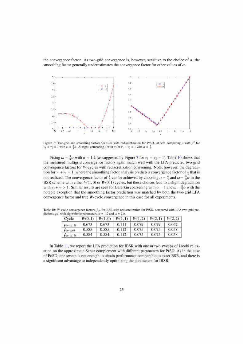
the convergence factor. As two-grid convergence is, however, sensitive to the choice of α, thesmoothing factor generally underestimates the convergence factor for other values of α.

Figure 7: Two-grid and smoothing factors for BSR with rediscretization for PrSD. At left, comparing ρ with µ2 forν1 = ν2 = 1 with ω = 8

9α. At right, comparing ρ with µ for ν1 + ν2 = 1 with α = 45 .

Fixing ω = 89α with α = 1.2 (as suggested by Figure 7 for ν1 = ν2 = 1), Table 10 shows that

the measured multigrid convergence factors again match well with the LFA-predicted two-gridconvergence factors for W-cycles with rediscretization coarsening. Note, however, the degrada-tion for ν1 +ν2 = 1, where the smoothing factor analysis predicts a convergence factor of 1

3 that isnot realized. The convergence factor of 1

3 can be achieved by choosing α = 45 and ω = 8

9α in theBSR scheme with either W(1, 0) or W(0, 1) cycles, but these choices lead to a slight degradationwith ν1 +ν2 > 1. Similar results are seen for Galerkin coarsening with α = 1 and ω = 8

9αwith thenotable exception that the smoothing factor prediction was matched by both the two-grid LFAconvergence factor and true W-cycle convergence in this case for all experiments.

Table 10: W-cycle convergence factors, ρh, for BSR with rediscretization for PrSD, compared with LFA two-grid pre-dictions, ρh, with algorithmic parameters, α = 1.2 and ω = 8

9α.


In Table 11, we report the LFA prediction for IBSR with one or two sweeps of Jacobi relax-ation on the approximate Schur complement with different parameters for PrSD. As in the caseof PoSD, one sweep is not enough to obtain performance comparable to exact BSR, and there isa significant advantage to independently optimizing the parameters for IBSR.

25

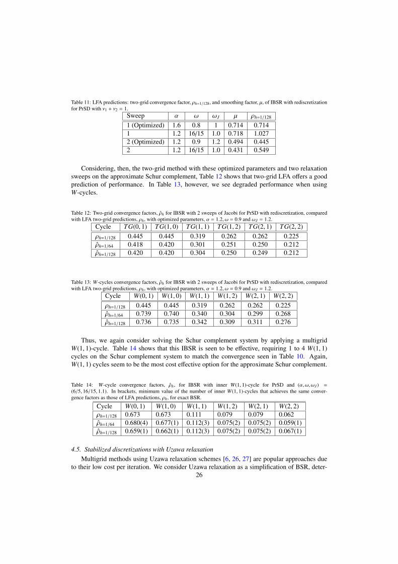
Table 11: LFA predictions: two-grid convergence factor, ρh=1/128, and smoothing factor, µ, of IBSR with rediscretizationfor PrSD with ν1 + ν2 = 1.

Sweep α ω ωJ µ ρh=1/128

1 (Optimized) 1.6 0.8 1 0.714 0.7141 1.2 16/15 1.0 0.718 1.0272 (Optimized) 1.2 0.9 1.2 0.494 0.4452 1.2 16/15 1.0 0.431 0.549

Considering, then, the two-grid method with these optimized parameters and two relaxationsweeps on the approximate Schur complement, Table 12 shows that two-grid LFA offers a goodprediction of performance. In Table 13, however, we see degraded performance when usingW-cycles.

Table 12: Two-grid convergence factors, ρh for IBSR with 2 sweeps of Jacobi for PrSD with rediscretization, comparedwith LFA two-grid predictions, ρh, with optimized parameters, α = 1.2, ω = 0.9 and ωJ = 1.2.

Cycle TG(0, 1) TG(1, 0) TG(1, 1) TG(1, 2) TG(2, 1) TG(2, 2)ρh=1/128 0.445 0.445 0.319 0.262 0.262 0.225ρh=1/64 0.418 0.420 0.301 0.251 0.250 0.212ρh=1/128 0.420 0.420 0.304 0.250 0.249 0.212

Table 13: W-cycles convergence factors, ρh for IBSR with 2 sweeps of Jacobi for PrSD with rediscretization, comparedwith LFA two-grid predictions, ρh, with optimized parameters, α = 1.2, ω = 0.9 and ωJ = 1.2.


Thus, we again consider solving the Schur complement system by applying a multigridW(1, 1)-cycle. Table 14 shows that this IBSR is seen to be effective, requiring 1 to 4 W(1, 1)cycles on the Schur complement system to match the convergence seen in Table 10. Again,W(1, 1) cycles seem to be the most cost effective option for the approximate Schur complement.

Table 14: W-cycle convergence factors, ρh, for IBSR with inner W(1, 1)-cycle for PrSD and (α, ω, ωJ) =

(6/5, 16/15, 1.1). In brackets, minimum value of the number of inner W(1, 1)-cycles that achieves the same conver-gence factors as those of LFA predictions, ρh, for exact BSR.

Cycle W(0, 1) W(1, 0) W(1, 1) W(1, 2) W(2, 1) W(2, 2)ρh=1/128 0.673 0.673 0.111 0.079 0.079 0.062ρh=1/64 0.680(4) 0.677(1) 0.112(3) 0.075(2) 0.075(2) 0.059(1)ρh=1/128 0.659(1) 0.662(1) 0.112(3) 0.075(2) 0.075(2) 0.067(1)

4.5. Stabilized discretizations with Uzawa relaxationMultigrid methods using Uzawa relaxation schemes [6, 26, 27] are popular approaches due

to their low cost per iteration. We consider Uzawa relaxation as a simplification of BSR, deter-26

mining the update as the (weighted) solution of

Mδx =

(αD 0B −S

) (δUδp

)=

(rUrp

),

where αD is an approximation to A and −S is an approximation of the Schur complement,−BA−1BT −C.

Here, we consider an analogue to exact BSR with D = diag(A). The choice of S is discussedlater. In this setting, we observe that minimizing the LFA smoothing factor does not minimizethe LFA convergence factor. Thus, we consider minimizing the two-grid convergence factornumerically for ν1 + ν2 = 1 and ν1 = ν2 = 1 with rediscretization coarsening, and compare withmeasured multigrid performance.

We consider three approximations to the Schur complement, starting from the true approx-imate Schur complement, C + B(αdiag(A))−1BT . Motivated by the stable finite-element case,we also consider replacing B(αdiag(A))−1BT in this matrix by a weighted mass matrix, yieldingS = C + δQ. Finally, motivated by the finite-difference case and efficiency of implementation,we consider taking S = σh2I, for a scalar weight, σ, to be optimized by the LFA. Note that, dueto the constant-coefficient stencils assumed by LFA, this corresponds to using a single sweep ofJacobi to approximate solution of either of the two above approximations.

For the case of C + B(αdiag(A))−1BT , the optimized LFA two-grid convergence factors forν1 + ν2 = 1 with rediscretization coarsening are 0.428 for PoSD and 0.436 for PrSD. These arenotably worse than the BSR smoothing factor of 1

3 , which is achieved for W(1, 0) or W(0, 1)cycles. Here, W(1, 0) cycles reflect this convergence, achieving measured convergence factorsof 0.417 for PoSD and 0.526 for PrSD. Increasing the number of relaxation sweeps per iterationyields some improvement in the predicted LFA convergence factors when optimizing parametersagain, but not enough to outperform repeated W(1, 0) cycles.

For the mass-matrix-based approximation, S = C + δQ, the optimized two-grid convergencefactors for ν1 + ν2 = 1 with rediscretization coarsening are 0.5 for PoSD and 0.417 for PrSD.While poorer convergence might be expected in both cases, the addition of an extra parameter, δ,allows a (slight) improvement for PrSD. In both cases, we observe consistent performance withnumerical experiments, achieving convergence factors of 0.493 for PoSD and 0.392 for PrSDusing W(0, 1) or W(1, 0) cycles.

Finally, for the diagonal approximation S = σh2I, we achieve notably better performanceoptimizing with ν1 = ν2 = 1 than for ν1 + ν2 = 1. For PoSD, the optimized two-grid LFAconvergence factor is 0.382, while it is 0.497 for PrSD. In practice, we achieve slightly worseconvergence factors using W(1, 1) cycles with rediscretization coarsening, of 0.531 for PoSD and0.543 for PrSD. These are both significantly worse than the convergence factors of 1

9 observedusing inexact BSR; however, it must be noted that W-cycles on the Schur complement systemwere needed in that case. A better approximation to inverting the true approximate Schur com-plement would be to apply multigrid to it, just as was done for IBSR above. Here, we observethat significant work may be needed to achieve convergence similar to that of Uzawa where theSchur complement is exactly inverted, requiring 10 W(1, 1)-cycles on the approximate Schurcomplement to achieve a convergence factor of 0.416 for PoSD and 0.522 for PrSD, suggestingthat the Jacobi version of Uzawa is ultimately more efficient.

4.6. Comparing cost and performanceFor convenience, we denote standard DWJ as DWJ(1) and DWJ with 2 sweeps of Jacobi

relaxation on the pressure equation as DWJ(2) in the following.27

The above results give a clear comparison of the effectiveness of the multigrid cycles with theconsidered relaxation schemes, but not of their relative efficiencies. To translate from effective-ness to efficiency, we must properly account for the cost per iteration of each relaxation scheme.All schemes assume the residual is already calculated; for the 9-point stencils in A, B, and stabi-lization terms, C, the cost of a single residual evaluation on a mesh with n points is (roughly) thatof 63n multiply-add operations, coming from the 7 nonzero blocks in the matrix. For DWJ(1),the rest of the cost of relaxation is fairly easy to account, requiring one diagonal scaling opera-tion on each of the three components of the solution vector, plus matrix-vector products with thepressure Laplacian, Ap, and with both B and BT . Counting multiply-add operations for these ona grid with n points, we have 3n for the diagonal scalings, and 9n each for the multiplication withAp and with Bx and By and their transposes, totalling 48n multiply-add operations. For DWJ(2),we need 48n multiply-add operators plus the cost of the second sweep. For the second sweep,we need to compute a residual related to G, the (3, 3) block of (11), and a diagonal scaling. Notethat the cost of the residual is 54n (9n each for the multiplication with Ap, C, and with Bx and By

and their transposes). In total, the cost of DWJ(2) is 103n multiply-add operators. For IBSR, fol-lowing (26), we require two diagonal scaling operations on each of the velocity components, onematrix-vector product with each of B and BT , and 2 or 3 W(1,1) cycles on the pressure variable.To account for the costs of the W(1,1) cycles, we use the standard cost estimate for W-cycles, asrequiring 4 “Work Units” per iteration, where a Work Unit is the cost of forming a residual for thepressure equation. Here, given the 25-point stencil structure seen in Equation (29), each WorkUnit requires 25 multiply-add operations, so the total cost of IBSR with 2 W(1,1) cycles on theSchur complement is 4n + 36n + 200n = 240n multiply-add operations (and 340n multiply-addoperations if 3 W(1,1) cycles are needed). Finally, Uzawa relaxation with diagonal scaling onthe pressure has a cost less than that of DWJ(1), as it requires diagonal scaling again for all threecomponents of the solution, but only one matrix-vector multiplication, with B. These total 21nmultiply-add operations.

Accumulating the costs of a residual evaluation with these, we have total costs of 111nmultiply-add operations per sweep of DWJ(1), 166n multiply-add operations per sweep of DWJ(2),303n multiply-add operations per sweep of IBSR with 2 W(1,1) cycles per Schur-complementsolve, and 84n multiply-add operations per sweep of Uzawa with diagonal scaling. Consideringthese relative to one-another, we see that DWJ(1) has a cost of about 4/3 per cycle as Uzawa, thatDWJ(2) has a per-cycle cost of about 2 times that of Uzawa, and 1.5 times that of DWJ(1), thatIBSR has a per-cycle cost of about 3.6 times that of Uzawa, 2.7 and 1.8 times that of DWJ(1) andDWJ(2), respectively. The per-cycle convergence factors observed above are 0.35 per cycle forW(1,1) cycles of DWJ(1) for PoSD and 0.44 per cycle for W(1,1) cycles of DWJ(1) for PrSD,0.11 per cycle for W(1,1) cycles of DWJ(2) and IBSR for both stabilizations, and 0.53 or 0.54per cycle for W(1,1) cycles with Uzawa. Comparing efficiencies can now be easily done by ap-propriately weighting these convergence factors relative to their work: if one iteration costs Wtimes that of another, and yields a convergence factor of ρ1, then we can easily compare ρ1/W

1directly to the second convergence factor, ρ2, to see if the effective error reduction achieved bythe first algorithm in an equal amount of work to the second is better or worse than that achievedby the second. Comparing DWJ(1) to Uzawa, then, for PoSD, we compare 0.353/4 ≈ 0.46 to0.53 and see that DWJ(1) is more efficient. For PrSD, we compare 0.443/4 ≈ 0.54 and see thatDWJ(1) and Uzawa are similarly efficient for PrSD. Comparing DWJ(2) to Uzawa, we compare0.111/2 ≈ 0.33 to 0.53(0.54), showing that DWJ(2) is much efficient than Uzawa. ComparingDWJ(2) to DWJ(1), we compare 0.111/1.5 ≈ 0.23 to 0.35 (0.45) and see DWJ(2) is more efficientthan DWJ(1). Comparing IBSR to Uzawa, we compare 0.111/3.6 ≈ 0.54, and see that it as also

28

comparable in efficiency to the others for the case of PrSD, but slightly less efficient than DWJ(1)for PoSD. DWJ(2) and IBSR have the same per-cycle convergence factor, but the cost of DWJ(2)(166n) is less than IBSR (303n). Thus DWJ(2) is more efficient than IBSR. Overall, DWJ(2)outperforms Uzawa, IBSR and DWJ(1). We note that these results are a little different than thoseseen for the MAC discretization in [18], where IBSR outperforms other schemes. Differencesseen in practice (and the influence of factors ignored in the LFA, such as boundary conditions)are important to consider.

An important practical consideration commonly observed in the LFA literature (see, for ex-ample, [18, 35]) is the influence of boundary conditions. In numerical experiments not shownhere, we often see significant degradation in convergence between the results for periodic bound-ary conditions and those for Dirichlet boundary conditions, particularly for cases with largernumbers of relaxation sweeps per cycle. For DWJ(2) with ν1 + ν2 = 1, changing from periodicto Dirichlet boundary conditions results in convergence factors increasing from 0.324 reportedin Tables 2 and 4 to about 0.46 (PrSD) or 0.56 (PoSD) for two-grid cycles, and to about 0.64(PrSD) and 0.7 (PoSD) for W-cycles. For IBSR with ν1 + ν2 = 1, however, the degradation ismuch less, with W-cycle convergence rates of 0.38 for PoSD (still with 2 inner W(1,1)-cyclesfor the Schur complement system) and 0.35 for PrSD (with α = 4/5, ω = 32/45, and 4 W(1,1)cycles with ωJ = 1.1 for the Schur complement system). Clearly this difference in performanceis enough to change the balance above, with the added cost of IBSR with inner W-cycles payingoff over DWJ(2).

5. Relaxation for Q2 − Q1 discretization

As explored in [15], classical LFA smoothing factor analysis is unreliable for Q2 discretiza-tions, making it unsuitable for analysis of the standard stable Q2−Q1 discretization of the Stokesequations. Thus, we consider only numerical (“brute force”) optimization of two-grid LFA con-vergence factors in this setting.

For DWJ, we find optimal convergence factors of 0.619 for ν1 + ν2 = 1 and 0.558 for ν1 =

ν2 = 1. While the former is quite comparable to convergence predicted and achieved for bothstabilized discretizations with ν1+ν2 = 1, we see a significant lack of improvement with increasedrelaxation, in contrast to the equal-order case. The same is observed for multigrid W-cycleperformance, with W(1, 0) convergence measured at 0.620 and W(1, 1) convergence measured at0.510.

For exact BSR, we find optimal convergence factors of 0.551 for ν1 + ν2 = 1 and 0.250 forν1 = ν2 = 1. While these are slightly larger than the comparable factors of 1

3 and 19 , respectively,

for the stabilized discretizations, they still reflect good performance of the underlying method.At left of Figure 8, we show the spectral radius of the error-propagation symbol for exact BSR

as a function of Fourier frequency, θ, noting that predicted reduction over the high frequenciesis not as good as would be needed to equal two-grid convergence in the equal-order case. Inorder to see how the convergence factor changes with the parameters α and ω, we display theconvergence factor as a function of α and ω at the right of Figure 8. The optimal choice, ofα = 1.1 and ω = 1.05, occurs in a narrow band of ω values, but larger range of α values lead toreasonable results.

29

Figure 8: At left, the spectral radius of the error-propagation symbol for exact BSR applied to the Q2 −Q1 discretization,as a function of the Fourier mode, θ. At right, the LFA-predicted two-grid convergence factor for BSR applied to theQ2 − Q1 discretization as a function of α and ω, with (ν1, ν2) = (1, 1).

As always, an inexact solve of the Schur complement system is needed to yield a practicalvariant of BSR. While 2 sweeps of Jacobi appears sufficient to achieve scalable W-cycle con-vergence when ν1 + ν2 > 2 (see Table 15), we find 3 sweeps are needed to achieve W(1, 1)convergence factors of 0.240 (see Table 16), in contrast to results in [21] and for the equal-orderdiscretizations considered here, where a much stronger iteration was needed. Similar results wereseen for V(1, 1) cycles when 3 sweeps of Jacobi were used for the Schur complement system.

Table 15: W-cycles convergence factors, ρh, for IBSR with 2 sweeps Jacobi for Q2−Q1 approximation with rediscretiza-tion, compared with LFA two-grid predictions, ρh, for exact BSR with algorithmic parameters, α = 1.1, ω = 1.05 andωJ = 1.0.

Cycle W(0, 1) W(1, 0) W(1, 1) W(1, 2) W(2, 1) W(2, 2)ρh=1/128 4.893 4.893 0.249 0.109 0.109 0.090ρh=1/64 NAN NAN 0.434 0.131 0.130 0.085ρh=1/128 NAN NAN 0.437 0.130 0.130 0.085

Table 16: W-cycles convergence factors, ρh, for IBSR with 3 sweeps Jacobi for Q2−Q1 approximation with rediscretiza-tion, compared with LFA two-grid predictions, ρh, for exact BSR with algorithmic parameters, α = 1.1, ω = 1.05 andωJ = 1.0.

Cycle W(0, 1) W(1, 0) W(1, 1) W(1, 2) W(2, 1) W(2, 2)ρh=1/128 4.893 4.893 0.249 0.109 0.109 0.090ρh=1/64 491.373 492.094 0.240 0.104 0.104 0.085ρh=1/128 NAN NAN 0.240 0.104 0.104 0.085

Finally, we consider the same three variants of Uzawa relaxation as examined above for theequal-order case. For S = B(αdiag(A))−1BT , the best convergence factor found for ν1 + ν2 = 1was 0.729, while better convergence was predicted for S = δQ, with factor 0.554. This is tobe expected, perhaps, since the Q1 mass matrix is well-known to be a better approximation of

30

the true Schur complement than the classical BSR approximate Schur complement. However,approximating either by a single sweep of Jacobi, yielding S = σh2I, gives a convergence factor0.717. While 2-grid cycles with ν1 + ν2 = 1 match the predicted convergence factor, W-cyclesdid not converge for these parameters.

Comparing, then, the efficiency of inexact BSR and DWJ for the Q2 − Q1 discretization,we see that inexact BSR, where W(1, 1) cycles achieve a convergence factor of 0.24 providesroughly the same reduction as 3 cycles with 1 DWJ sweep per cycle, where LFA predicts ρ =

0.619. Noting that inexact BSR is relatively more expensive in this case, with cost dominatedby the two diagonal scalings per sweep on the Q2 velocity degrees of freedom, we suggest aproper implementation study is needed to determine which, if either, provides best performancein practice.

6. Conclusion

In this paper, LFA is presented for block-structured relaxation schemes for stabilized andstable finite-element discretizations of the Stokes equations. The convergence and smoothingfactors exhibited here provide optimized parameters for DWJ with one or two sweeps of Jacobirelaxation on the pressure equation and BSR for the stabilized discretizations. The convergenceof (inexact) BSR clearly outperforms multigrid with both standard DWJ and Uzawa relaxation.However, standard DWJ can be improved by additional relaxation on the pressure equation,and the improved version is more efficient than IBSR. While the LFA smoothing factor loses itspredictivity of the two-grid convergence factor for the stable Q2−Q1 discretization and for Uzawarelaxation for both stabilized and stable discretizations, the two-grid LFA convergence factorcan still provide useful predictions. We consider as well the inexact case for BSR, with Jacobiiterations or multigrid cycles used to approximate solution of the Schur complement system, asis suitable for use on modern parallel and graphics processing unit (GPU) architectures. Fromnumerical experiments, we see that inexact BSR can be as good as the exact iteration for solvingthe Stokes equations. The analysis and LFA predictions demonstrated here offer good insightinto the use of block-structured relaxation for other types of saddle-point problems, which willbe considered in future work.

Acknowledgements

The work of S.M. was partially supported by an NSERC discovery grant.

References

[1] H. C. Elman, D. J. Silvester, A. J. Wathen, Finite elements and fast iterative solvers with applications in incom-pressible fluid dynamics, 2nd Edition, Numerical Mathematics and Scientific Computation, Oxford UniversityPress, Oxford, 2014.

[2] J. W. Ruge, K. Stuben, Algebraic multigrid, Multigrid methods 3 (13) (1987) 73–130.[3] J. Adler, T. R. Benson, E. Cyr, S. P. MacLachlan, R. S. Tuminaro, Monolithic multigrid methods for two-

dimensional resistive magnetohydrodynamics, SIAM J. Sci. Comput. 38 (1) (2016) B1–B24.[4] J. H. Adler, D. B. Emerson, S. P. MacLachlan, T. A. Manteuffel, Constrained optimization for liquid crystal equi-

libria, SIAM J. Sci. Comput. 38 (1) (2016) B50–B76.[5] A. Brandt, N. Dinar, Multigrid solutions to elliptic flow problems, in: Numerical methods for partial differential

equations, Vol. 42 of Publ. Math. Res. Center Univ. Wisconsin, Academic Press, New York-London, 1979, pp.53–147.

[6] M. A. Olshanskii, Multigrid analysis for the time dependent Stokes problem, Math. Comp. 81 (277) (2012) 57–79.31

[7] J. Schoberl, W. Zulehner, On Schwarz-type smoothers for saddle point problems, Numer. Math. 95 (2) (2003)377–399.

[8] J. H. Adler, T. R. Benson, S. P. MacLachlan, Preconditioning a mass-conserving discontinuous Galerkin discretiza-tion of the Stokes equations, Numer. Linear Algebra Appl. 24 (3) (2017) e2047, 23.

[9] P. E. Farrell, L. Mitchell, F. Wechsung, An augmented lagrangian preconditioner for the 3D stationary incompress-ible Navier-Stokes equations at high Reynolds number, arXiv preprint arXiv:1810.03315.

[10] U. Trottenberg, C. W. Oosterlee, A. Schuller, Multigrid, Academic Press, Inc., San Diego, CA, 2001, with contri-butions by A. Brandt, P. Oswald and K. Stuben.

[11] R. Wienands, W. Joppich, Practical Fourier analysis for multigrid methods, CRC press, 2004.[12] A. Brandt, Rigorous quantitative analysis of multigrid, I. constant coefficients two-level cycle with L2-norm, SIAM

Journal on Numerical Analysis 31 (6) (1994) 1695–1730.[13] R. P. Stevenson, On the validity of local mode analysis of multi-grid methods, Ph.D. thesis (1990).[14] C. Rodrigo, F. J. Gaspar, L. T. Zikatanov, On the validity of the local Fourier analysis, Journal of Computational

Mathematics 37 (3) (2019) 340–348.[15] Y. He, S. P. MacLachlan, Two-level Fourier analysis of multigrid for higher-order finite-element methods, submit-

ted.[16] S. P. MacLachlan, C. W. Oosterlee, Local Fourier analysis for multigrid with overlapping smoothers applied to

systems of PDEs, Numer. Linear Algebra Appl. 18 (4) (2011) 751–774.[17] S. Friedhoff, S. MacLachlan, C. Borgers, Local Fourier analysis of space-time relaxation and multigrid schemes,

SIAM Journal on Scientific Computing 35 (5) (2013) S250–S276.[18] Y. He, S. P. MacLachlan, Local Fourier analysis of block-structured multigrid relaxation schemes for the Stokes

equations, Numerical Linear Algebra with Applications 25 (3), e2147.[19] D. Braess, R. Sarazin, An efficient smoother for the Stokes problem, Appl. Numer. Math. 23 (1) (1997) 3–19.[20] D. Braess, W. Dahmen, A cascadic multigrid algorithm for the Stokes equations, Numer. Math. 82 (2) (1999)

179–191.[21] W. Zulehner, A class of smoothers for saddle point problems, Computing 65 (3) (2000) 227–246.[22] S. P. Vanka, Block-implicit multigrid solution of Navier-Stokes equations in primitive variables, J. Comput. Phys.

65 (1) (1986) 138–158.[23] S. Manservisi, Numerical analysis of Vanka-type solvers for steady Stokes and Navier-Stokes flows, SIAM J.

Numer. Anal. 44 (5) (2006) 2025–2056.[24] C. Rodrigo, F. J. Gaspar, F. J. Lisbona, On a local Fourier analysis for overlapping block smoothers on triangular

grids, Appl. Numer. Math. 105 (2016) 96–111.[25] L. John, U. Rude, B. Wohlmuth, W. Zulehner, On the analysis of block smoothers for saddle point problems, arXiv

preprint arXiv:1612.01333.[26] F. J. Gaspar, Y. Notay, C. W. Oosterlee, C. Rodrigo, A simple and efficient segregated smoother for the discrete

Stokes equations, SIAM J. Sci. Comput. 36 (3) (2014) A1187–A1206.[27] B. Gmeiner, M. Huber, L. John, U. Rude, B. Wohlmuth, A quantitative performance study for Stokes solvers at the

extreme scale, J. Comput. Sci. 17 (part 3) (2016) 509–521.[28] J.-F. Maitre, F. Musy, P. Nigon, A fast solver for the Stokes equations using multigrid with a Uzawa smoother,

in: Advances in multigrid methods (Oberwolfach, 1984), Vol. 11 of Notes Numer. Fluid Mech., Vieweg+TeubnerVerlag, Wiesbaden, 1985, pp. 77–83.

[29] C. Bacuta, P. S. Vassilevski, S. Zhang, A new approach for solving Stokes systems arising from a distributiverelaxation method, Numerical Methods for Partial Differential Equations 27 (4) (2011) 898–914.

[30] G. Wittum, Multi-grid methods for Stokes and Navier-Stokes equations, Numer. Math. 54 (5) (1989) 543–563.[31] M. Wang, L. Chen, Multigrid methods for the Stokes equations using distributive Gauss-Seidel relaxations based

on the least squares commutator, J. Sci. Comput. 56 (2) (2013) 409–431.[32] C. W. Oosterlee, F. J. Gaspar, Multigrid methods for the Stokes system, Computing in Science & Engineering 8 (6)

(2006) 34–43.[33] L. Chen, Multigrid methods for saddle point systems using constrained smoothers, Comput. Math. Appl. 70 (12)

(2015) 2854–2866.[34] S. Takacs, A robust multigrid method for the time-dependent Stokes problem, SIAM J. Numer. Anal. 53 (6) (2015)

2634–2654.[35] A. Niestegge, K. Witsch, Analysis of a multigrid Stokes solver, Appl. Math. Comput. 35 (3) (1990) 291–303.[36] S. Sivaloganathan, The use of local mode analysis in the design and comparison of multigrid methods, Computer

Physics Communications 65 (1-3) (1991) 246–252.[37] J. Molenaar, A two-grid analysis of the combination of mixed finite elements and Vanka-type relaxation, in: Multi-

grid methods, III (Bonn, 1990), Vol. 98 of Internat. Ser. Numer. Math., Birkhauser, Basel, 1991, pp. 313–323.[38] A. J. Wathen, T. Rees, Chebyshev semi-iteration in preconditioning for problems including the mass matrix, Elec-

tronic Transactions on Numerical Analysis 34 (125-135) (2009) 125–135.

32

[39] A. Wathen, D. Silvester, Fast iterative solution of stabilised Stokes systems. part I: Using simple diagonal precon-ditioners, SIAM J. Numer. Anal. 30 (3) (1993) 630–649.

[40] D. Silvester, A. Wathen, Fast iterative solution of stabilised Stokes systems part II: using general block precondi-tioners, SIAM J. Numer. Anal. 31 (5) (1994) 1352–1367.

[41] S. C. Brenner, L. R. Scott, The mathematical theory of finite element methods, 3rd Edition, Vol. 15 of Texts inApplied Mathematics, Springer, New York, 2008.

[42] F. Brezzi, J. Douglas, Stabilized mixed methods for the Stokes problem, Numer. Math. 53 (1) (1988) 225–235.[43] C. R. Dohrmann, P. B. Bochev, A stabilized finite element method for the Stokes problem based on polynomial

pressure projections, International Journal for Numerical Methods in Fluids 46 (2) (2004) 183–201.[44] L. Chen, X. Hu, M. Wang, J. Xu, A multigrid solver based on distributive smoother and residual overweighting for

Oseen problems, Numerical Mathematics: Theory, Methods and Applications 8 (02) (2015) 237–252.[45] J. H. Adler, D. Emerson, S. P. MacLachlan, T. A. Manteuffel, Constrained optimization for liquid crystal equilibria,

SIAM Journal on Scientific Computing 38 (1) (2016) B50–B76.

33

local fourier analysis for mixed ﬁnite-element methods for...

Documents