local invariant feature detectors: a surveyepubs.surrey.ac.uk/726872/1/tuytelaars-fgv-2008.pdf ·...
TRANSCRIPT

Foundations and TrendsR© inComputer Graphics and VisionVol. 3, No. 3 (2007) 177–280c© 2008 T. Tuytelaars and K. MikolajczykDOI: 10.1561/0600000017
Local Invariant Feature Detectors: A Survey
Tinne Tuytelaars1 and Krystian Mikolajczyk2
1 Department of Electrical Engineering, Katholieke Universiteit Leuven,Kasteelpark Arenberg 10, B-3001 Leuven, Belgium,[email protected]
2 School of Electronics and Physical Sciences, University of Surrey,Guildford, Surrey, GU2 7XH, UK, [email protected]
Abstract
In this survey, we give an overview of invariant interest point detectors,how they evolved over time, how they work, and what their respectivestrengths and weaknesses are. We begin with defining the properties ofthe ideal local feature detector. This is followed by an overview of theliterature over the past four decades organized in different categories offeature extraction methods. We then provide a more detailed analysisof a selection of methods which had a particularly significant impact onthe research field. We conclude with a summary and promising futureresearch directions.
1Introduction
In this section, we discuss the very nature of local (invariant) fea-tures. What do we mean with this term? What is the advantage ofusing local features? What can we do with them? What would the ideallocal feature look like? These are some of the questions we attempt toanswer.
1.1 What are Local Features?
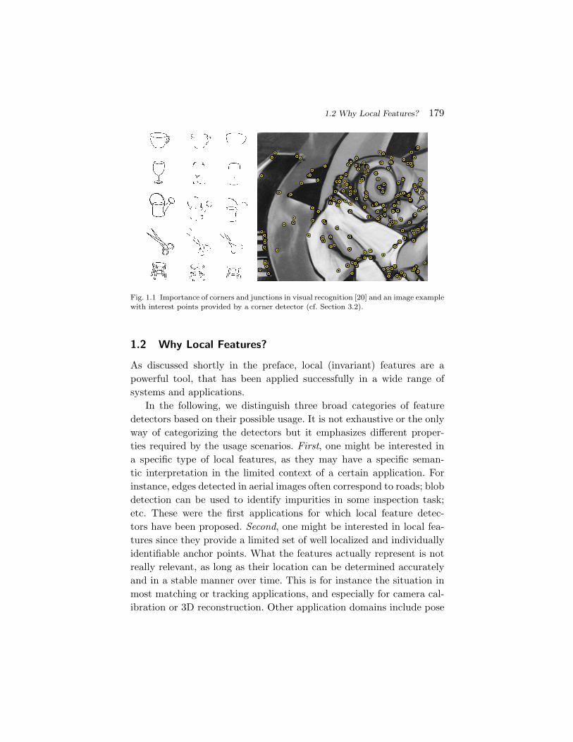
A local feature is an image pattern which differs from its immediateneighborhood. It is usually associated with a change of an image prop-erty or several properties simultaneously, although it is not necessarilylocalized exactly on this change. The image properties commonly con-sidered are intensity, color, and texture. Figure 1.1 shows some exam-ples of local features in a contour image (left) as well as in a grayvalueimage (right). Local features can be points, but also edgels or smallimage patches. Typically, some measurements are taken from a regioncentered on a local feature and converted into descriptors. The descrip-tors can then be used for various applications.
178
1.2 Why Local Features? 179
Fig. 1.1 Importance of corners and junctions in visual recognition [20] and an image examplewith interest points provided by a corner detector (cf. Section 3.2).
1.2 Why Local Features?
As discussed shortly in the preface, local (invariant) features are apowerful tool, that has been applied successfully in a wide range ofsystems and applications.
In the following, we distinguish three broad categories of featuredetectors based on their possible usage. It is not exhaustive or the onlyway of categorizing the detectors but it emphasizes different proper-ties required by the usage scenarios. First, one might be interested ina specific type of local features, as they may have a specific seman-tic interpretation in the limited context of a certain application. Forinstance, edges detected in aerial images often correspond to roads; blobdetection can be used to identify impurities in some inspection task;etc. These were the first applications for which local feature detec-tors have been proposed. Second, one might be interested in local fea-tures since they provide a limited set of well localized and individuallyidentifiable anchor points. What the features actually represent is notreally relevant, as long as their location can be determined accuratelyand in a stable manner over time. This is for instance the situation inmost matching or tracking applications, and especially for camera cal-ibration or 3D reconstruction. Other application domains include pose

180 Introduction
estimation, image alignment or mosaicing. A typical example here arethe features used in the KLT tracker [228]. Finally, a set of local featurescan be used as a robust image representation, that allows to recognizeobjects or scenes without the need for segmentation. Here again, itdoes not really matter what the features actually represent. They donot even have to be localized precisely, since the goal is not to matchthem on an individual basis, but rather to analyze their statistics. Thisway of exploiting local features was first reported in the seminal workof [213] and [210] and soon became very popular, especially in thecontext of object recognition (both for specific objects as well as forcategory-level recognition). Other application domains include sceneclassification, texture analysis, image retrieval, and video mining.
Clearly, each of the above three categories imposes its own con-straints, and a good feature for one application may be useless in thecontext of a different problem. These categories can be considered whensearching for suitable feature detectors for an application at hand. Inthis survey, we mainly focus on the second and especially the thirdapplication scenario.
Finally, it is worth noting that the importance of local featureshas also been demonstrated in the context of object recognition bythe human visual system [20]. More precisely, experiments have shownthat removing the corners from images impedes human recognition,while removing most of the straight edge information does not. This isillustrated in Figure 1.1.
1.3 A Few Notes on Terminology
Before we discuss feature detectors in more detail, let us explain someterminology commonly used in the literature.
1.3.1 Detector or Extractor?
Traditionally, the term detector has been used to refer to the tool thatextracts the features from the image, e.g., a corner, blob or edge detec-tor. However, this only makes sense if it is a priori clear what thecorners, blobs or edges in the image are, so one can speak of “falsedetections” or “missed detections.” This only holds in the first usage

1.3 A Few Notes on Terminology 181
scenario mentioned earlier, not for the last two, where extractor wouldprobably be semantically more correct. Still, the term detector is widelyused. We therefore also stick to this terminology.
1.3.2 Invariant or Covariant?
A similar discussion holds for the use of “invariant” or “covariant.”A function is invariant under a certain family of transformations ifits value does not change when a transformation from this family isapplied to its argument. A function is covariant when it commuteswith the transformation, i.e., applying the transformation to the argu-ment of the function has the same effect as applying the transformationto the output of the function. A few examples may help to explain thedifference. The area of a 2D surface is invariant under 2D rotations,since rotating a 2D surface does not make it any smaller or bigger. Butthe orientation of the major axis of inertia of the surface is covariantunder the same family of transformations, since rotating a 2D sur-face will affect the orientation of its major axis in exactly the sameway. Based on these definitions, it is clear that the so-called local scaleand/or affine invariant features are in fact only covariant. The descrip-tors derived from them, on the other hand, are usually invariant, due toa normalization step. Since the term local invariant feature is so widelyused, we nevertheless use “invariant” in this survey.
1.3.3 Rotation Invariant or Isotropic?
A function is isotropic at a particular point if it behaves the same inall directions. This is a term that applies to, e.g., textures, and shouldnot be confused with rotational invariance.
1.3.4 Interest Point, Region or Local Feature?
In a way, the ideal local feature would be a point as defined in geometry:having a location in space but no spatial extent. In practice however,images are discrete with the smallest spatial unit being a pixel anddiscretization effects playing an important role. To localize features inimages, a local neighborhood of pixels needs to be analyzed, giving

182 Introduction
all local features some implicit spatial extent. For some applications(e.g., camera calibration or 3D reconstruction) this spatial extent iscompletely ignored in further processing, and only the location derivedfrom the feature extraction process is used (with the location sometimesdetermined up to sub-pixel accuracy). In those cases, one typically usesthe term interest point.
However, in most applications those features also need to bedescribed, such that they can be identified and matched, and this againcalls for a local neighborhood of pixels. Often, this neighborhood istaken equal to the neighborhood used to localize the feature, but thisneed not be the case. In this context, one typically uses the term regioninstead of interest point. However, beware: when a local neighborhoodof pixels is used to describe an interest point, the feature extractionprocess has to determine not only the location of the interest point,but also the size and possibly the shape of this local neighborhood.Especially in case of geometric deformations, this significantly compli-cates the process, as the size and shape have to be determined in aninvariant (covariant) way.
In this survey, we prefer the use of the term local feature, which canbe either points, regions or even edge segments.
1.4 Properties of the Ideal Local Feature
Local features typically have a spatial extent, i.e., the local neigh-borhood of pixels mentioned above. In contrast to classical segmen-tation, this can be any subset of an image. The region boundariesdo not have to correspond to changes in image appearance such ascolor or texture. Also, multiple regions may overlap, and “uninter-esting” parts of the image such as homogeneous areas can remainuncovered.
Ideally, one would like such local features to correspond to seman-tically meaningful object parts. In practice, however, this is unfeasible,as this would require high-level interpretation of the scene content,which is not available at this early stage. Instead, detectors select localfeatures directly based on the underlying intensity patterns.

1.4 Properties of the Ideal Local Feature 183
Good features should have the following properties:
• Repeatability: Given two images of the same object or scene,taken under different viewing conditions, a high percentageof the features detected on the scene part visible in bothimages should be found in both images.
• Distinctiveness/informativeness: The intensity patternsunderlying the detected features should show a lot of varia-tion, such that features can be distinguished and matched.
• Locality: The features should be local, so as to reduce theprobability of occlusion and to allow simple model approx-imations of the geometric and photometric deformationsbetween two images taken under different viewing conditions(e.g., based on a local planarity assumption).
• Quantity: The number of detected features should be suffi-ciently large, such that a reasonable number of features aredetected even on small objects. However, the optimal numberof features depends on the application. Ideally, the numberof detected features should be adaptable over a large rangeby a simple and intuitive threshold. The density of featuresshould reflect the information content of the image to providea compact image representation.
• Accuracy: The detected features should be accurately local-ized, both in image location, as with respect to scale andpossibly shape.
• Efficiency: Preferably, the detection of features in a newimage should allow for time-critical applications.
Repeatability, arguably the most important property of all, can beachieved in two different ways: either by invariance or by robustness.
• Invariance: When large deformations are to be expected,the preferred approach is to model these mathematically ifpossible, and then develop methods for feature detection thatare unaffected by these mathematical transformations.
• Robustness: In case of relatively small deformations, it oftensuffices to make feature detection methods less sensitive to

184 Introduction
such deformations, i.e., the accuracy of the detection maydecrease, but not drastically so. Typical deformations thatare tackled using robustness are image noise, discretizationeffects, compression artifacts, blur, etc. Also geometric andphotometric deviations from the mathematical model usedto obtain invariance are often overcome by including morerobustness.
1.4.1 Discussion
Clearly, the importance of these different properties depends on theactual application and settings, and compromises need to be made.
Repeatability is required in all application scenarios and it directlydepends on the other properties like invariance, robustness, quantityetc. Depending on the application increasing or decreasing them mayresult in higher repeatability.
Distinctiveness and locality are competing properties and cannot befulfilled simultaneously: the more local a feature, the less information isavailable in the underlying intensity pattern and the harder it becomesto match it correctly, especially in database applications where thereare many candidate features to match to. On the other hand, in case ofplanar objects and/or purely rotating cameras (e.g., in image mosaicingapplications), images are related by a global homography, and there areno problems with occlusions or depth discontinuities. Under these con-ditions, the size of the local features can be increased without problems,resulting in a higher distinctiveness.
Similarly, an increased level of invariance typically leads to areduced distinctiveness, as some of the image measurements are used tolift the degrees of freedom of the transformation. A similar rule holdsfor robustness versus distinctiveness, as typically some information isdisregarded (considered as noise) in order to achieve robustness. Asa result, it is important to have a clear idea on the required level ofinvariance or robustness for a given application. It is hard to achievehigh invariance and robustness at the same time and invariance, whichis not adapted to the application, may have a negative impact on theresults.

1.5 Global versus Local Features 185
Accuracy is especially important in wide baseline matching, regis-tration, and structure from motion applications, where precise corre-spondences are needed to, e.g., estimate the epipolar geometry or tocalibrate the camera setup.
Quantity is particularly useful in some class-level object or scenerecognition methods, where it is vital to densely cover the object ofinterest. On the other hand, a high number of features has in mostcases a negative impact on the computation time and it should be keptwithin limits. Also robustness is essential for object class recognition,as it is impossible to model the intra-class variations mathematically, sofull invariance is impossible. For these applications, an accurate local-ization is less important. The effect of inaccurate localization of a fea-ture detector can be countered, up to some point, by having an extrarobust descriptor, which yields a feature vector that is not affected bysmall localization errors.
1.5 Global versus Local Features
Local invariant features not only allow to find correspondences in spiteof large changes in viewing conditions, occlusions, and image clutter(wide baseline matching), but also yield an interesting description ofthe image content for image retrieval and object or scene recognitiontasks (both for specific objects as well as categories). To put this intocontext, we briefly summarize some alternative strategies to computeimage representations including global features, image segments, andexhaustive and random sampling of features.
1.5.1 Global Features
In the field of image retrieval, many global features have been proposedto describe the image content, with color histograms and variationsthereof as a typical example [237]. This approach works surprisinglywell, at least for images with distinctive colors, as long as it is the overallcomposition of the image as a whole that the user is interested in, ratherthan the foreground object. Indeed, global features cannot distinguishforeground from background, and mix information from both partstogether.

186 Introduction
Global features have also been used for object recognition, result-ing in the first appearance-based approaches to tackle this challengingproblem. Turk and Pentland [245] and later Murase and Nayar [160]proposed to compute a principal component analysis of a set ofmodel images and to use the projections onto the first few principalcomponents as descriptors. Compared to the purely geometry-basedapproaches tried before, the results of the novel appearance-basedapproach were striking. A whole new range of natural objects couldsuddenly be recognized. However, being based on a global description,image clutter and occlusions again form a major problem, limiting theusefulness of the system to cases with clean backgrounds or where theobject can be segmented out, e.g., relying on motion information.
1.5.2 Image Segments
An approach to overcome the limitations of the global features is tosegment the image in a limited number of regions or segments, witheach such region corresponding to a single object or part thereof. Thebest known example of this approach is the blobworld system, pro-posed in [31], which segments the image based on color and texture,then searches a database for images with similar “image blobs.” Anexample based on texture segmentation is the wide baseline matchingwork described in [208].
However, this raises a chicken-and-egg problem as image segmen-tation is a very challenging task in itself, which in general requires ahigh-level understanding of the image content. For generic objects, colorand texture cues are insufficient to obtain meaningful segmentations.
1.5.3 Sampled Features
A way to deal with the problems encountered with global features orimage segmentations, is to exhaustively sample different subparts ofthe image at each location and scale. For each such image subpart,global features can then be computed. This approach is also referredto as a sliding window based approach. It has been especially popu-lar in the context of face detection, but has also been applied for the

1.5 Global versus Local Features 187
recognition of specific objects or particular object classes such as pedes-trians or cars.
By focusing on subparts of the image, these methods are able to findsimilarities between the queries and the models in spite of changingbackgrounds, and even if the object covers only a small percentageof the total image area. On the downside, they still do not manage tocope with partial occlusions, and the allowed shape variability is smallerthan what is feasible with a local features based approach. However, byfar the biggest drawback is the inefficiency of this approach. Each andevery subpart of the image must be analyzed, resulting in thousandsor even millions of features per image. This requires extremely efficientmethods which significantly limits the scope of possible applications.
To overcome the complexity problems more sparse fixed grid sam-pling of image patches was used (e.g., [30, 62, 246, 257]). It is howeverdifficult to achieve invariance to geometric deformations for such fea-tures. The approach can tolerate some deformations due to dense sam-pling over possible locations, scales, poses etc. 00, but the individualfeatures are not invariant. An example of such approach are multi-scaleinterest points. As a result, they cannot be used when the goal is tofind precise correspondences between images. However, for some appli-cations such as scene classification or texture recognition, they maywell be sufficient. In [62], better results are reported with a fixed gridof patches than with patches centered on interest points, in the contextof scene classification work. This can be explained by the dense cover-age, as well as the fact that homogeneous areas (e.g., sky) are also takeninto account in the fixed grid approach which makes the representationmore complete. This dense coverage is also exploited in [66], where afixed grid of patches was used on top of a set of local invariant featuresin the context of specific object recognition, where the latter supplyan initial set of correspondences, which then guide the construction ofcorrespondences for the former.
In a similar vein, rather than using a fixed grid of patches, a randomsampling of image patches can also be used (e.g., [97, 132, 169]). Thisgives a larger flexibility in the number of patches, the range of scales orshapes, and their spatial distribution. Good scene recognition resultsare shown in [132] based on random image patches. As in the case of

188 Introduction
fixed grid sampling, this can be explained by the dense coverage whichignores the localization properties of features. Random patches are infact a subset of the dense patches, and are used mostly to reduce thecomplexity. Their repeatability is poor hence they work better as anaddition to the regular features rather than as a stand alone method.
Finally, to overcome the complexity problems while still providing alarge number of features with better than random localization [140, 146]proposed to sample features uniformly from edges. This proved usefulfor dealing with wiry objects well represented by edges and curves.
1.6 Overview of this Survey
This survey article consists of two parts. First, in Section 2, we reviewlocal invariant feature detectors in the literature, from the early days incomputer vision up to the most recent evolutions. Next, we describe afew selected, representative methods in more detail. We have structuredthe methods in a relatively intuitive manner, based on the type offeature extracted in the image. Doing so, we distinguish between cornerdetectors (Section 3), blob detectors (Section 4), and region detectors(Section 5). Additionally, we added a section on various detectors thathave been designed in a computationally efficient manner (Section 6).With this structure, we hope the reader can easily find the type ofdetector most useful for his/her application. We conclude the surveywith a qualitative comparison of the different methods and a discussionof future work (Section 7).
To the novice reader, who is not very familiar with local invariantfeature detectors yet, we advice to skip Section 2 at first. This sectionhas been added mainly for the more advanced reader, to give furtherinsight in how this field evolved and what were the most importanttrends and to add pointers to earlier work.

2Local Features in the Literature
In this section, we give an overview of local feature detectors proposedin the literature, starting from the early days of image processing andpattern recognition up to the current state-of-the-art.
2.1 Introduction
The literature on local feature detection is vast and goes back as far as1954, when it was first observed by Attneave [6] that information onshape is concentrated at dominant points having high curvature. It isimpossible to describe each and every contribution to over 50 years ofresearch in detail. Instead, we provide pointers to the literature wherethe interested reader can find out more. The main goal of this sectionis to make the reader aware of the various great ideas that have beenproposed, especially in the pre-internet era. All too often, these areoverlooked and then re-invented. We would like to give proper creditto all those researchers who contributed to the current state-of-the-art.
2.1.1 Early Work on Local Features
It is important to mention the beginnings of this research areaand the first publications which appeared after the observation on
189

190 Local Features in the Literature
the importance of corners and junctions in visual recognition [6](see Figure 1.1). Since then a large number of algorithms have been sug-gested for extracting interest points at the extrema of various functionscomputed on the digital shape. Also, it has been understood early onin the image processing and visual pattern recognition field that inter-sections of straight lines and straight corners are strong indications ofman made structures. Such features have been used in a first seriesof applications from line drawing images [72] and photomosaics [149].First monographs on digital image processing by Rosenfeld [191] andby Duda and Hart [58] as well as their later editions served to establishthe field on a sound theoretical foundation.
2.1.2 Overview
We identified a number of important research directions and struc-tured the subsections of this section accordingly. First, many authorshave studied the curvature of contours to find corners. Their work isdescribed in Section 2.2. Others directly analyze the image intensities,e.g., based on derivatives or regions with high variance. This is the topicof Section 2.3. Another line of research has been inspired by the humanvisual system and aims at reproducing the processes in the humanbrain — see Section 2.4. Methods focussing on the exploitation of colorinformation are discussed in Section 2.5, while Section 2.6 describesmodel-based approaches. More recently, there has been a trend towardfeature detection with invariance against various geometric transfor-mations, including multi-scale approaches and scale or affine invariantmethods. These are discussed in Section 2.7. In Section 2.8, we focus onsegmentation-based methods and Section 2.9 describes methods whichbuild on machine learning techniques. Finally, Section 2.10 gives anoverview of different evaluation and comparison schemes proposed inthe literature.
2.2 Contour Curvature Based Methods
A first category of interest point detectors are the contour curvaturebased methods. Originally, these were mainly applied to line drawings,piecewise constant regions, and cad–cam images rather than natural

2.2 Contour Curvature Based Methods 191
scenes. The focus was especially on the accuracy of point localization.They were most popular of the end of the 1970s and most of the 1980s.
2.2.1 High Curvature Points
Contour intersections and junctions often result in bi-directional sig-nal changes. Therefore, a good strategy to detect features consists ofextracting points along the contour with high curvature. Curvature ofan analog curve is defined as the rate at which the unit tangent vec-tor changes with respect to arc length. Contours are often encoded inchains of points or represented in a parametric form using splines.
Several techniques have been developed which involve detecting andchaining edges so as to find corners in the chain by analyzing the chaincode [205], finding maxima of curvature [108, 136, 152], change in direc-tion [83], or change in appearance [42]. Others avoid chaining edges andinstead look for maxima of curvature [254] or change in direction [104]at places where the gradient is large.
Several methods for detecting edges based on gray-level gradient andangular changes in digital curves were proposed in [193, 195, 196, 197].Other solutions for line-drawing images include methods for detectingcorners in a chain-coded plane curve [73, 74]. In these works, a mea-sure for the cornerness of a point is based on mean angular differencesbetween successive segment positions along the chain.
One general approach to feature extraction is to detect the dominantpoints directly through angle or corner detection, using various schemesfor approximating discrete curvature such as cosine [192, 193] or localcurvature [18, 74] which define corners as discontinuities of an averagecurve slope. Other parametric representation like B-splines curves arecommonly used in rendering a curve in computer graphics, compressionand coding, CAD–CAM systems, and also for curve fitting and shapedescription [175]. In [108], cubic polynomials are fit to a curve anddiscontinuities are detected in such curve to localize interest points.Spline approximations of line images are used in [85] in combinationwith a dynamic programming technique to find the knots of a spline.Pseudo coding of line figures and a complicated vector finder to obtaininterest points are proposed in [164].

192 Local Features in the Literature
In [207], dominant points are computed at the maximum globalcurvature, based on the iterative averaging of local discretized curvatureat each point with respect to its immediate neighbors. In [3], tangentialdeflection and curvature of discrete curves are defined based on thegeometrical and statistical properties associated with the eigenvalue–eigenvector structure of sample covariance matrices computed on chain-codes.
Another approach is to obtain a piecewise linear polygonal approx-imation of the digital curve subject to certain constraints on the qual-ity of fit [60, 174, 176]. Indeed, it has been pointed out in [174] thatpiecewise linear polygonal approximation with variable breakpoints willtend to locate vertices at actual corner points. These points correspondapproximately to the actual or extrapolated intersections of adjacentline segments of the polygons. A similar idea was explored in [91]. Morerecently, [95] estimates the parameters of two lines fitted to the twosegments neighboring to the corner point. A corner is declared if theparameters are statistically significantly different. A similar approach isto identify edge crossings and junctions [19] by following image gradientmaxima or minima and finding gaps in edge maps.
2.2.2 Dealing with Scale
Corner detection methods by curvature estimation normally use a setof parameters to eliminate contour noise and to obtain the corners ata given scale, although object corners can be found at multiple nat-ural scales. To solve this problem, some detectors apply their algo-rithms iteratively within a certain range of parameters, selecting pointswhich appear in a fixed set of iterations. The stability of the points andthe time spent for their detection is closely related to the number ofiterations.
Initial attempts to deal with discretization and scale problems viaan averaging scheme can be found in [207]. The curvature primalsketch (CPS) proposed in [5] is a scale-space representation of signif-icant changes in curvature along contours. The changes are classifiedas basic or compound primitives such as corners, smooth joints, ends,cranks, bumps, and dents. The features are detected at different scales,

2.2 Contour Curvature Based Methods 193
resulting in a multiple-scale representation of object contours. A similaridea was explored in [151, 152] and later in [86], where the curvaturescale space analysis was performed to find the local scale of curves. Theyfind inflection points of the curves and represent shapes in parametricforms. A B-spline based algorithm was also proposed in [108, 136]. Thegeneral idea is to fit a B-Spline to the curve, then to measure the cur-vature around each point directly from the B-spline coefficients.
Another algorithm [238] dealing with scale for detecting dominantpoints on a digital closed curve is motivated by the angle detection pro-cedure from [193]. They indicate that the detection of dominant pointsrelies primarily on the precise determination of the region of supportrather than on the estimation of discrete curvature. First, the region ofsupport for each point based on its local properties is determined. Thena measure of relative curvature [238] or local symmetry [170] of eachpoint is computed. The Gaussian filter is the most commonly used filterin point detection. However, if the scale of a Gaussian filter is too small,the result may include some redundant points which are unnecessarydetails, i.e., due to noise. If the scale is too large, the points with smallsupport regions will tend to be smoothed out. To solve the problemsexisting in Gaussian filtering with fixed scale, scale-space proceduresbased on multiple-scale discrete curvature representation and search-ing are proposed in [4, 181]. The scheme is based on a stability criterionthat states that the presence of a corner must concur with a curvaturemaximum observable at a majority of scales. Natural scales of curveswere studied in [199] to avoid exhaustive representation of curves over afull range of scales. A successful scale selection mechanism for Gaussianfilters with a theoretical formulation was also proposed in [119, 120].
In [264] a nonlinear algorithm for critical point detection is pre-sented. They establish a set of criteria for the design of a point detectionalgorithm to overcome the problems arising from curvature approxima-tion and Gaussian filtering. Another approach to boundary smoothingis based on simulated annealing for curvature estimation [233]. In [152]the corner points are localized at the maxima of absolute curvatureof edges. The corner points are tracked through multiple curvaturescale levels to improve localization. Chang and Horng [33] proposed analgorithm to detect corner points using a nest moving average filter
194 Local Features in the Literature
is investigated in [33]. Corners are detected on curves by computingthe difference of blurred images and observing the shift of high curva-ture points. More detailed analysis of various methods for determiningnatural scales of curves can be found in [125, 199, 200].
2.2.3 Discussion
Although theoretically well founded for analog curves, the contour cur-vature calculation is less robust in case of discrete curves [194, 238].Possible error sources in digital curvature estimation were investigatedin [259].
Furthermore, the objectives for the above discussed detectors weredifferent than the ones we typically have nowadays. It was considereddisadvantageous if a method detected corners on circular shapes, mul-tiple corners at junctions etc. At that time, a much stricter definitionof interest points/corners was used, with only points correspondingto true corners in 3D being considered as relevant. Nowadays, inmost practical applications of interest points, the focus is on robust,stable, and distinctive points, irrespective of whether they corre-spond to true corners or not (see also our earlier discussion inSection 1.2).
There has been less activity in this area recently (over the pastten years), due to complexity and robustness problems, while methodsbased directly on image intensity attracted more attention.
2.3 Intensity Based Methods
Methods based on image intensity have only weak assumptions andare typically applicable to a wide range of images. Many of theseapproaches are based on first- and second-order gray-value derivatives,while others use heuristics to find regions of high variance.
2.3.1 Differential Approaches
Hessian-based approaches. One of the early intensity based detec-tors is the rotation invariant Hessian-based detector proposed by

2.3 Intensity Based Methods 195
Beaudet [16]. It explores the second-order Taylor expansion of the inten-sity surface, and especially the Hessian matrix (containing the secondorder derivatives). The determinant of this matrix reaches a maximumfor blob-like structures in the image. A more detailed description ofthis method can be found in Section 4.1. It has been extended in [57]and [266], where the interest points are localized at the zero crossingof a curve joining local extrema of the Hessian determinant arounda corner.
Similarly, high curvature points can be localized by computingGaussian curvature of the image surface, i.e., saddle points in imagebrightness. In [104], a local quadratic surface was fit to the image inten-sity function. The parameters of the surface were used to determine thegradient magnitude and the rate of change of gradient direction. Theresulting detector uses the curvature of isophotes computed from first-and second-order derivatives scaled by image gradient to make it morerobust to noise. A similar idea was proposed in [61, 229].
A detailed investigation in [168, 167, 224] and later in [83] showsthat the detectors of [16, 57, 104, 163, 266] all perform the samemeasurements on the image and have relatively low reliability accord-ing to criteria based on localization precision. Nevertheless, the traceand determinant of the Hessian matrix were successfully used lateron in scale and affine invariant extensions of interest point detec-tors [121, 143] when other feature properties became more important.
Gradient-based approaches. Local feature detection based on first-order derivatives is also used in various applications. A corner detectorwhich returns points at the local maxima of a directional variance mea-sure was first introduced in [154, 155, 156] in the context of mobile robotnavigation. It was a heuristic implementation of the auto-correlationfunction also explored in [41]. The proposed corner detector investigatesa local window in the image and determines the average change of inten-sity which results from shifting the window by a few pixels in variousdirections. This idea is taken further in [69, 70] and formalized by usingfirst-order derivatives in a so-called second moment matrix to explorelocal statistics of directional image intensity variations. The methodseparates corner candidate detection and localization to improve the

196 Local Features in the Literature
accuracy to subpixel precision, at the cost of higher computational com-plexity. Harris and Stephens [84] improved the approach by Moravec[155] by performing analytical expansion of the average intensity vari-ance. This results in a second moment matrix computed with Sobelderivatives and a Gaussian window. A function based on the determi-nant and trace of that matrix was introduced which took into accountboth eigenvalues of the matrix. This detector is widely known todayas the Harris detector or Plessey detector,1 and is probably the bestknown interest point detector around. It is described in more detailin Section 3.2. It has been extended in numerous papers, e.g., byusing Gaussian derivatives [212], combinations of first- and second-order derivatives [263], or an edge based second moment matrix [45]but the underlying idea remains the same.
The Harris detector was also investigated in [167] and demonstratedto be optimal for L junctions. Based on the assumption of an affineimage deformation, an analysis in [228] led to the conclusion that it ismore convenient to use the smallest eigenvalue of the autocorrelationmatrix as the corner strength function.
More recently, the second moment matrix has also been adoptedto scale changes [59] by parameterizing Gaussian filters and normaliz-ing them with respect to scale, based on scale-space theory [115, 117].Also, the Harris detector was extended with search over scale and affinespace in [13, 142, 209], using the Laplacian operator and eigenvalues ofthe second moment matrix, inspired by the pioneering work of Linde-berg [117, 118] (see Section 3.4 for details).
The approach from [263] performs an analysis of the computationof the second moment matrix and its approximations. A speed increaseis achieved by computing only two smoothed images, instead of thethree previously required. A number of other suggestions have beenmade for how to compute the corner strength from the second-ordermatrix [84, 101, 167, 228], and these have all been shown to be equiv-alent to various matrix norms [102, 265]. A generalization to imageswith multi-dimensional pixels was also proposed in [102].
1 Plessey Electronic Research Ltd.

2.3 Intensity Based Methods 197
In [242], the Harris corner detector is extended to yield stable fea-tures under more general transformations than pure translations. Tothis end, the auto-correlation function was studied under rotations,scalings, up to full affine transformations.
2.3.2 Intensity Variations
A different category of approaches based on intensity variations appliesmathematical morphology to extract high curvature points. The useof zero-crossings of the shape boundary curvature in binary images,detected with a morphological opening operator was investigatedin [36]. Mathematical morphology was also used to extract convex andconcave points from edges in [107, 114, 168]. Later on a parallel algo-rithm based on an analysis of morphological residues and corner char-acteristics was proposed in [262].
Another approach [173] indicates that for interest points the medianvalue over a small neighborhood is significantly different from thecorner point value. Thus the difference in intensity between thecenter and median gives a strong indication for corners. However,this method cannot deal with more complex junctions or smoothedges.
A simple and efficient detector named SUSAN was introducedin [232] based on earlier work from [82]. It computes the fraction ofpixels within a neighborhood which have similar intensity to the centerpixel. Corners can then be localized by thresholding this measure andselecting local minima. The position of the center of gravity is used tofilter out false positives. More details on the SUSAN detector can befound in Section 3.3. A similar idea was explored in [112, 240] wherepixels on a circle are considered and compared to the center of a patch.
More recently, [203] proposed the FAST detector. A point is clas-sified as a corner if one can find a sufficiently large set of pixels on acircle of fixed radius around the point such that these pixels are allsignificantly brighter (resp. darker) than the central point. Efficientclassification is based on a decision tree. More details on FAST can befound in Section 6.3.

198 Local Features in the Literature
Local radial symmetry has been explored in [127] to identify interestpoints and its real-time implementation was also proposed. Wavelettransformation was also investigated in the context of feature pointextraction with successful results based on multi-resolution analysisin [35, 111, 218].
2.3.3 Saliency
The idea of saliency has been used in a number of computer visionalgorithms. The early approach of using edge detectors to extract objectdescriptions embodies the idea that the edges are more significant thanother parts of the image. More explicit uses of saliency can be dividedinto those that concentrate on low-level local features (e.g., [215]), andthose that compute salient groupings of low-level features (e.g., [223]);though some approaches operate at both levels (e.g., [147]).
The technique suggested in [211], is based on the maximization ofdescriptor vectors across a particular image. These salient points arethe points on the object which are almost unique. Hence they maxi-mize the discrimination between the objects. A related method [253]identifies salient features for use in automated generation of StatisticalShape/Appearance Models. The method aims to select those featureswhich are less likely to be mismatched. Regions of low density in a mul-tidimensional feature space, generated from the image, are classified ashighly salient.
A more theoretically founded approach based on variability or com-plexity of image intensity within a region was proposed in [79]. It wasmotivated by visual saliency and information content, which we revisein the next section. The method from [79] defines saliency in terms oflocal signal complexity or unpredictability; more specifically the use ofShannon entropy of local attributes is suggested. The idea is to find apoint neighborhood with high complexity as a measure of saliency orinformation content. The method measures the change in entropy of agray-value histogram computed in a point neighborhood. The searchwas extended to scale [98] and affine [99] parameterized regions, thusproviding position, scale, and affine shape of the region neighborhood.For a detailed discussion, we refer to Section 4.3.

2.4 Biologically Plausible Methods 199
2.4 Biologically Plausible Methods
Most systems proposed in the previous sections were mainly concernedwith the accuracy of interest point localization. This is important in thecontext of fitting parametric curves to control points or image match-ing for recovering the geometry. In contrast, the biologically plausiblemethods reviewed in this section were mainly proposed in the con-text of artificial intelligence and visual recognition. Most of them didnot have a specific application purpose and their main goal was tomodel the processes of the human brain. Numerous models of humanvisual attention or saliency have been discussed in Cognitive Psychol-ogy and Computer Vision. However, the vast majority were only oftheoretical interest and only few were implemented and tested on realimages.
2.4.1 Feature Detection as Part of the Pre-attentive Stage
One of the main models for early vision in humans, attributed toNeisser [165], is that it consists of a pre-attentive and an atten-tive stage. Biologically plausible methods for feature detection usu-ally refer to the idea that certain parts of a scene are pre-attentivelydistinctive and create some form of immediate response within theearly stages of the human visual system. In the pre-attentive stage,only “pop-out” features are detected. These are local regions of theimage which present some form of spatial discontinuity. In the atten-tive stage, relationships between these features are found, and group-ing takes place. This model has widely influenced the computervision community (mainly through the work of Marr [133]) and isreflected in the classical computer vision approach — feature detec-tion and perceptual grouping, followed by model matching and corre-spondence search. Activities in the models of attention started in themid-1980s following progress in neurophysiological and psychologicalresearch.
One approach inspired by neuro-biological mechanisms was pro-posed in [87, 198]. They apply Gabor like filters to compute localenergy of the signal. Maxima of the first- and second-order deriva-tives of that energy indicate the presence of interest points. The idea of

200 Local Features in the Literature
using Gabor filter responses from different scales was further exploredin [131, 186]. The approach developed in [182] was motivated by psy-chophysical experiments. They compute a symmetry score of the signalat each image pixel in different directions. Regions with significant sym-metry are then selected as interest points.
Theory on texture recognition and the idea of textons as simple localstructures like blobs, corners, junctions, line ends etc. was introducedin [96]. He suggested that statistics over texton distributions play animportant role in recognition. The extraction of simple textons is donein the pre-attentive stage and the construction of relations in the atten-tive stage. A feature integration theory based on these principles wasproposed in [241]. He distinguished between a disjunctive case wherethe distinctive features can be directly localized in a feature map and aconjunctive case where the feature can be extracted only by processingvarious feature maps simultaneously. This model was implemented bycombining bottom up and top down measures of interest [32]. The bot-tom up method merges various feature maps and looks for interestingevents, while in the top down process, knowledge about the target isexploited.
The main goal of the above systems was to provide computation-ally plausible models of visual attention. Their interest was mainlytheoretical. However, those systems served as source of inspiration forpractical solutions for real images once machine learning techniqueslike neural networks had grown mature enough. In [206], image pro-cessing operators were combined with the attentive models to make itapplicable to more realistic images. He applies a Laplacian-of-Gaussians(LoG) like operator to feature maps to model the receptive fields andenhance the interesting events. The image was analyzed at multiplescales. The approach from [78] uses a set of feature templates and cor-relates them with the image to produce feature maps which are thenenhanced with LoG. Temporal derivatives were used to detect movingobjects.
Koch and Ullman [105] proposed a very influential computationalmodel of visual attention which accounts for several psychophysicalphenomena. They proposed to build a set of maps based on orienta-tion, color, disparity and motion, and to simulate the lateral inhibition

2.4 Biologically Plausible Methods 201
mechanism by extracting locations which differ significantly from theirneighborhood. Information from different maps is then merged into asingle saliency map. A winner-take-all (WTA) network was used toselect the active location in the maps in a hierarchical manner using apyramidal strategy. The hypotheses suggested in [105, 241] were firstimplemented in [34]. A similar implementation of the WTA model wasproposed in [49].
The extraction of globally salient structures like object outlines wasinvestigated in [223] by grouping local information such as contourfragments but no relation to pre-attentive vision was claimed.
2.4.2 Non-uniform Resolution and Coarse-To-FineProcessing
Also non-uniform resolution of the retina and coarse-to-fine process-ing strategies have been studied in biologically plausible models. Thesehave been simulated mostly via scale-space techniques [9, 10, 187, 255].However, these systems were mostly focused on the engineering andrealtime aspects rather than its biological plausibility. One of the firstsystems to perform interest point detection in scale-space was pro-posed in [27]. They built a Laplacian pyramid for coarse-to-fine fea-ture selection. Templates were used to localize the objects in the LoGspace. Templates were also employed for building features maps whichwere then combined by a weighted sum [39]. Difference-of-Gaussians(DoG) filters were used in the system designed in [76] to accelerate thecomputation.
Biologically inspired systems developed in [81] explored the idea ofusing boundary and interest point detectors based on DoG filters aswell as directional differences of offset Gaussians (DOOG) to simulatesimple cells in V1.
The system proposed in [130] was mainly concerned with classifi-cation of textures studied earlier in [96]. The feature extraction partused a bank of filters based on oriented kernels (DoG and DOOG) toproduce feature maps similar to [81]. The next stage corresponds toa WTA mechanism to suppress weak responses and simulate lateral
202 Local Features in the Literature
inhibition. Finally, all the responses are merged to detect textureboundaries.
2.4.3 Spatial Event Detection
Robust statistics have also been used to detect outliers in a set ofimage primitives. The idea is based on the observation that texturescan be represented by their statistics and the locations which violatethose statistics represent interesting events. For example, texture prim-itives are represented by a number of attributes using histograms andRANSAC in [148].
First order statistics over feature maps computed from zero cross-ings of DoG at different scales are used in [23]. For each point, ahistogram of gradient orientations is then constructed, and the localhistograms are combined into a global one, which is similar in spirit tothe more recent SIFT descriptor [124, 126]. Local histograms are thencompared with the global one to provide a measure of interest.
Another statistical model was proposed in [172]. They measure theedge density at a range of distances from the interest point to build anedge distribution histogram. This idea has been used later in the shapecontext descriptor of [17].
Cells that respond only to edges and bars which terminate withintheir receptive field have first been found in [92]. A corner detectionalgorithm based on a model for such end-stopped cells in the visual cor-tex was presented in [87, 260]. Furthermore, the notion of end-stoppedcells was generalized to color channels in a biologically plausible waybased on color opponent processes [260].
A more recent visual attention system also motivated by the earlyprimate visual system, is presented in [94]. Multiscale image featuresdetected at local spatial discontinuities in intensity, color, and orien-tation are combined into a single topographical saliency map and aneural network selects locations depending on the saliency.
Other recent visual recognition systems inspired by a model of visualcortex V1 which follow models from [185] can be found in [162, 221,222]. These methods attempt to implement simple and complex cells

2.5 Color-based Methods 203
from visual cortex which are multiscale Gabor and edgel detectors fol-lowed by local maxima selection methods.
2.5 Color-based Methods
Color provides additional information which can be used in theprocess of feature extraction. Several biologically plausible methodsreviewed in the previous section use color for building saliencymaps [93, 94, 105, 260].
Given the high performance of Harris corners [84], a straightforwardextension of the second moment matrix to RGB color space was intro-duced in [80, 153], incorporating color information in the Harris cornerextraction process.
Salient point detection based on color distinctiveness has been pro-posed in [250]. Salient points are the maxima of the saliency map, whichrepresents distinctiveness of color derivatives in a point neighborhood.In related work [217] they argue that the distinctiveness of color-basedsalient points is much higher than for the intensity ones. Color ratiosbetween neighboring pixels are used to obtain derivatives independentof illumination, which results in color interest points that are morerobust to illumination changes.
Most of the proposed approaches based on color are simple exten-sions of methods based on the intensity change. Color gradients areusually used to enhance or to validate the intensity change so as toincrease the stability of the feature detectors but the pixel intensitiesremain the main source of information for feature detection.
2.6 Model-based Methods
There have been a few attempts to do an analytical study of cornerdetection by giving a formal representation of corner points in an imagebased on differential geometry techniques [82] or contour curvature [53].For instance, it was found that a gray-level corner point can be found asthe point of maximal planar curvature on the line of the steepest gray-level slope [82, 188]. An analytical expression for an optimal function

204 Local Features in the Literature
whose convolution with an image has significant values at corner pointswas investigated in [180].
The methods presented in [82, 201] assume that a corner resem-bles a blurred wedge, and finds the characteristics of the wedge (theamplitude, angle, and blur) by fitting it to the local image. Several mod-els of junctions of multiple edges were used in [188]. The assumption isthat the junctions are formed by homogeneous regions. Parameterizedmasks are used to fit the intensity structure including position, orienta-tion, intensity, blurring, and edges. The residual is then minimized dur-ing the detection. The accuracy is high provided a good initializationof the parameters. The efficiency of the approach in [188] was improvedin [52] by using a different blurring function and a method to initializethe parameters. Fitting a corner model to image data was also consid-ered in [137, 171]. For each possible intersection of lines a template wasconstructed based on the angle, orientation, and scale of the hypothe-sized corner. The template was then matched to the image in a smallneighborhood of the interest point to verify the model. A template-based method for locating the saddle-points was also described in [128],where the corner points correspond to the intersections of saddle-ridgeand saddle-valley structures.
A set of fuzzy patterns of contour points were established in [113]and the corner detection was characterized as a fuzzy classificationproblem of the patterns.
Other model-based methods, aimed at improving the detectionaccuracy of the Hessian-based corner detector [16], were proposed in[54, 266]. To this end, the responses of the corner detector on a the-oretical model over scale-space were analyzed. It was observed thatthe operator responses at different scales move along the bisector line.It is worth to note that this observation is also valid for the pop-ular Harris corner detector [84]. The exact position of the cornerwas then computed from two responses indicating the bisector andits intersection with the zero-crossing of the Laplacian response. Anaffine transformation was also used to fit a model of a corner to animage [22].
A different model-based approach is proposed in [77]. For each typeof feature, a parametric model is developed to characterize the local

2.7 Toward Viewpoint Invariant Methods 205
intensity in an image. Projections of intensity profile onto a set oforthogonal Zernike moment-generating polynomials are used to esti-mate model-parameters and generate the feature map.
An interesting technique is to find corners by fitting a parameterizedmodel with the Generalized Hough transform [51, 226]. In images withextracted edges two lines appear in a parameter space for each cornerand the peak occurs at the crossover. Real corner models in the formof templates were considered in [229]. A similarity measure and severalalternative matching schemes were applied. Detection and localizationaccuracy was improved by merging the output of the different matchingtechniques.
In general, only relatively simple feature models were considered inthe above methods and the generalization to images other than polyg-onal is not obvious. The complexity is also a major drawback in suchapproaches.
2.7 Toward Viewpoint Invariant Methods
Most of the detectors described so far extract features at a single scale,determined by the internal parameters of the detector. At the end of the1990s, as local features were more and more used in the context of widebaseline matching and object recognition, there was a growing needfor features that could cope with scale changes or even more generalviewpoint changes.
2.7.1 Multi-Scale Methods
Most of the detectors described so far extract features at a single scale,determined by the internal parameters of the detector. To deal withscale changes, a straightforward approach consists of extracting pointsover a range of scales and using all these points together to repre-sent the image. This is referred to as a multi-scale or multi-resolutionapproach [48].
In [59], a scale adapted version of the Harris operator was proposed.Interest points are detected at the local maxima of the Harris functionapplied at several scales. Thanks to the use of normalized derivatives,a comparable strength of the cornerness measure is obtained for points

206 Local Features in the Literature
detected at different scales, such that a single threshold can be used toreject less significant corners over all scales. This scale adapted detectorsignificantly improves the repeatability of interest points under scalechanges. On the other hand, when prior knowledge on the scale changebetween two images is given, the detector can be adapted so as toextract interest points only at the selected scales. This yields a set ofpoints, for which the respective localization and scale perfectly reflectthe real scale change between the images.
In general, multi-scale approaches suffer from the same problemsas dense sampling of features (cf. Section 1.5). They cannot cope wellwith the case where a local image structure is present over a rangeof scales, which results in multiple interest points being detected ateach scale within this range. As a consequence, there are many points,which represent the same structure, but with slightly different localiza-tion and scale. The high number of points increases the ambiguity andthe computational complexity of matching and recognition. Therefore,efficient methods for selecting accurate correspondences and verifyingthe results are necessary at further steps of the algorithms. In contrastto structure from motion applications, this is less of an issue in thecontext of recognition where a single point can have multiple correctmatches.
2.7.2 Scale-Invariant Detectors
To overcome the problem of many overlapping detections, typicalof multiscale approaches, scale-invariant methods have been intro-duced. These automatically determine both the location and scaleof the local features. Features are typically circular regions, in thatcase.
Many existing methods search for maxima in the 3D representationof an image (x,y and scale). This idea for detecting local features inscale-space was introduced in the early 1980s [47]. The pyramid repre-sentation was computed with low pass filters. A feature point is detectedif it is at a local maximum of a surrounding 3D cube and if its abso-lute value is higher than a certain threshold. Since then many methodsfor selecting points in scale-space have been proposed. The existing

2.7 Toward Viewpoint Invariant Methods 207
approaches mainly differ in the differential expression used to build thescale-space representation.
A normalized LoG function was applied in [116, 120] to build ascale space representation and search for 3D maxima. The scale-spacerepresentation is constructed by smoothing the high resolution imagewith derivatives of Gaussian kernels of increasing size. Automatic scaleselection (cf. Section 3.4) is performed by selecting local maxima inscale-space. The LoG operator is circularly symmetric. It is thereforenaturally invariant to rotation. It is also well adapted for detecting blob-like structures. The experimental evaluation in [138] shows this functionis well suited for automatic scale selection. The scale invariance of inter-est point detectors with automatic scale selection has also been exploredin [24]. Corner detection and blob detection with automatic scale selec-tion were also proposed in a combined framework in [24] for featuretracking with adaptation to spatial and temporal size variations. Theinterest point criterion that is being optimized for localization need notbe the same as the one used for optimizing the scale. In [138], a scale-invariant corner detector, coined Harris-Laplace, and a scale-invariantblob detector, coined Hessian-Laplace were introduced. In these meth-ods, position and scale are iteratively updated until convergence [143].More details can be found in Sections 3.4 and 4.2.
An efficient algorithm for object recognition based on local 3Dextrema in the scale-space pyramid built with DoG filters was intro-duced in [126]. The local 3D extrema in the pyramid representationdetermine the localization and the scale of interest points. This methodis discussed further in Section 6.1.
2.7.3 Affine Invariant Methods
An affine invariant detector can be seen as a generalization of thescale-invariant ones to non-uniform scaling and skew, i.e., with adifferent scaling factor in two orthogonal directions and without pre-serving angles. The non-uniform scaling affects not only the localiza-tion and the scale but also the shape of characteristic local structures.Therefore, scale-invariant detectors fail in the case of significant affinetransformations.

208 Local Features in the Literature
Affine invariant feature detection, matching, and recognition havebeen addressed frequently in the past [50, 90, 204]. Here, we focus onthe methods which deal with invariant interest point detection.
One category of approaches was concerned with the localizationaccuracy under affine and perspective transformations. An affine invari-ant algorithm for corner localization was proposed in [2] which buildson the observations made in [54]. Affine morphological multi-scale anal-ysis is applied to extract corners. The evolution of a corner is given by alinear function formed by the scale and distance of the detected pointsfrom the real corner. The location and orientation of the corner is com-puted based on the assumption that the multiscale points move alongthe bisector line and the angle indicates the true location. However,in natural scenes a corner can take any form of a bi-directional signalchange and in practice the evolution of a point rarely follows the bisec-tor. The applicability of the method is therefore limited to a polygonallike world.
Other approaches were concerned with simultaneous detection oflocation, size and affine shape of local structures. The method intro-duced in [247], coined EBR (Edge-Based Regions) starts from Harriscorners and nearby intersecting edges. Two points moving along theedges together with the Harris point determine a parallelogram. Thepoints stop at positions where some photometric quantities of the tex-ture covered by the parallelogram reach an extremum. The methodcan be categorized as a model-based approach as it looks for a specificstructure in images, albeit not as strict as most methods described inSection 2.6. More details can be found in Section 3.5. A similar schemehas been explored in [12].
An intensity-based method (IBR, Intensity-Based Regions) wasalso proposed in [248]. It starts with the extraction of local inten-sity extrema. The intensity profiles along rays emanating from a localextremum are investigated. A marker is placed on each ray in the place,where the intensity profile significantly changes. Finally, an ellipse isfitted to the region determined by the markers. This method is furtherdiscussed in Section 5.1. Somewhat similar in spirit are the MaximallyStable Extremal Regions or MSER proposed in [134] and described inthe next section.

2.7 Toward Viewpoint Invariant Methods 209
A method to find blob-like affine invariant features using an iter-ative scheme was introduced in [121], in the context of shape fromtexture. This method based on the affine invariance of shape adaptedfixed points was also used for estimating surface orientation from binoc-ular data (shape from disparity gradients). The algorithm exploresthe properties of the second moment matrix and iteratively estimatesthe affine deformation of local patterns. It effectively estimates thetransformation that would project the patch to a frame in whichthe eigenvalues of the second moment matrix are equal. This workprovided a theoretical background for several other affine invariantdetectors.
It was combined with the Harris corner detector and used in thecontext of matching in [13], hand tracking in [109], fingerprint recog-nition [1] and for affine rectification of textured regions in [208]. In[13], interest points are extracted at several scales using the Harrisdetector and then the shape of the regions is adapted to the localimage structure using the iterative procedure from [118]. This allowsto extract affine invariant descriptors for a given fixed scale and loca-tion — that is, the scale and the location of the points are notextracted in an affine invariant way. Furthermore, the multi-scale Har-ris detector extracts many points which are repeated at the neighbor-ing scale levels. This increases the probability of a mismatch and thecomplexity.
The Harris-Laplace detector introduced in [141] was extendedin [142, 209] by affine normalization with the algorithm proposedin [13, 118, 121]. This detector suffers from the same drawbacks, asthe initial location and scale of points are not extracted in an affineinvariant way, although the uniform scale changes between the viewsare handled by the scale-invariant Harris-Laplace detector.
Beyond affine transformations. A scheme that goes even beyond affinetransformations and is invariant to projective transformations wasintroduced in [236]. However, on a local scale, the perspective effect isusually neglectable. More damaging is the effect of non-planarities ornon-rigid deformations. This is why a theoretical framework to extendthe use of local features to non-planar surfaces has been proposed in

210 Local Features in the Literature
[251], based on the definition of equivalence classes. However, in prac-tice, they have only shown results on straight corners. Simultaneously,an approach invariant to general deformations was developed in [122],by embedding an image as a 2D surface in 3D space and exploitinggeodesic distances.
2.8 Segmentation-based Methods
Segmentation techniques have also been employed in the context offeature extraction. These methods were either applied to find homoge-neous regions to localize junctions on their boundaries or to directlyuse these regions as local features. For the generic feature extrac-tion problem, mostly bottom-up segmentation based on low level pixelgrouping was considered, although in some specific tasks top-downmethods can also be applied. Although significant progress has beenmade in the analysis and formalization of the segmentation problem,it remains an unsolved problem in the general case. Optimal segmen-tation is intractable in general due to the large search space of possi-ble feature point groups, in particular in algorithms based on multipleimage cues. Moreover, a multitude of definitions of optimal segmen-tation even for the same image makes it difficult to solve. Nonethe-less, several systems using segmentation based interest regions havebeen developed, especially in the context of retrieval, matching, andrecognition.
In early years of computer vision polygonal approximations ofimages were popular in scene analysis and medical image analysis[9, 25, 58]. These algorithms often involved edge detection and sub-sequent edge following for region identification. In [63, 64], the verticesof a picture are defined as those points which are common in three ormore segmented regions. It can be seen as one of the first attemptsto extract interest points using segmentation. Simple segmentation ofpatches into two regions is used in [123] and the regions are comparedto find corners. Unfortunately, the two region assumption makes theusefulness of the method limited.
Another set of approaches represent real images through seg-mentation [129]. Well performing image segmentation methods are

2.9 Machine Learning-based Methods 211
based on graph cuts, where graphs represent connected image pix-els [21, 75, 225, 227]. These methods allow to obtain segmentationat the required level of detail. Although semantic segmentation is notreliable, over-segmenting the image can produce many regions whichfit to the objects. This approach was explored in [31, 46] and it is par-ticularly appealing for image retrieval problems where the goal is tofind similar images via regions with similar properties. In [44], the goalis to create interest operators that focus on homogeneous regions, andcompute local image descriptors for these regions. The segmentationis performed on several feature spaces using kernel-based optimiza-tion methods. The regions can be individually described and used forrecognition but their distinctiveness is low. This direction has recentlygained more interest and some approaches use bottom-up segmentationto extract interest regions or so-called superpixels [159, 184] (see alsoSection 5.3).
In general the disadvantages of this representation are that thesegmentation results are still unstable and inefficient for processinglarge amounts of images. An approach which successfully deals withthese problems was taken in [134]. Maximally Stable Extremal Regions(MSER) are extracted with a watershed like segmentation algorithm.The method extracts homogeneous intensity regions which are sta-ble over a wide range of thresholds. The regions are then replaced byellipses with the same shape moments up to the second-order. Recently,a variant of this method was introduced in [177], which handles theproblems with blurred region boundaries by using region isophotes.In a sense, this method is also similar to the IBR method describedin Section 5.1, as very similar regions are extracted. More detailson MSER can be found in Section 5.2. The method was extendedin [56, 161] with tree like representation of watershed evolution in theimage.
2.9 Machine Learning-based Methods
The progress in the domain of machine learning and the increase ofavailable computational power allowed learning techniques to enter thefeature extraction domain. The idea of learning the attributes of local

212 Local Features in the Literature
features from training examples and then using this information toextract features in other images has been around in the vision commu-nity for some time but only recently it was more broadly used in realapplications. The success of these methods is due to the fact that effi-ciency, provided by classifiers, became a more desirable property thanaccuracy of detection.
In [37, 55], a neural network is trained to recognize corners whereedges meet at a certain degree, near to the center of an image patch.This is applied to images after edge detection. A similar idea wasexplored in [244] to improve the stability of curvature measurementof digital curves.
Decision trees [178] have also been used successfully in interest pointdetection tasks. The idea of using intensity differences between the cen-tral points and neighboring points [173, 232, 240] has been adoptedin [202, 203]. They construct a decision tree to classify point neigh-borhoods into corners [203]. The main concern in their work is theefficiency in testing only a fraction of the many possible differencesand the tree is trained to optimize that. The approach of [203] was alsoextended with LoG filters to detect multiscale points in [112]. They usea feature selection technique based on the repeatability of individualinterest points over perspective projected images.
A hybrid methodology that integrates genetic algorithms anddecision tree learning in order to extract discriminatory features forrecognizing complex visual concepts is described in [11]. In [243], inter-est point detection is posed as an optimization problem. They use aGenetic Programming based learning approach to construct operatorsfor extracting features. The problem of learning an interest point oper-ator was posed differently in [103] where human eye movement wasstudied to find the points of fixation and to train an SVM classifier.
One can easily generalize the feature detection problem to a classifi-cation problem and train a recognition system on image examples pro-vided by one or a combination of the classical detectors. Any machinelearning approach can be used for that. Haar like filters implementedwith integral images to efficiently approximate multiscale derivativeswere used in [15]. A natural extension would be to use the learning

2.10 Evaluations 213
scheme from Viola and Jones [252] successfully applied to face detec-tion, to efficiently classify interest points.
The accuracy of machine learning based methods in terms of local-ization, scale, and shape estimation is in general lower than for thegeneric detectors [84, 134, 143] but in the context of object recognitionthe efficiency is usually more beneficial.
2.10 Evaluations
Given the multitude of interest point approaches the need for indepen-dent performance evaluations was identified early on and many exper-imental tests have been performed over the last three decades. Variousexperimental frameworks and criteria were used. One of the first com-parisons of corner detection techniques based on chain coded curves waspresented in [205]. In the early papers very often only visual inspec-tion was done [104]. Others performed more quantitative evaluationsproviding scores for individual images or for small test data [57, 266].
Corner detectors were often tested on artificially generated imageswith different types of junctions with varying angle, length, contrast,noise, blur etc. [41, 179]. Different affine photometric and geometrictransformations were used to generate the test data and to evaluatecorner detectors in [37, 100, 124, 128]. This approach simplifies theevaluation process but cannot model all the noise and deformationswhich affect the detector performance in a real application scenario,thus the performance results are often over-optimistic. A somewhatdifferent approach is taken in [150]. There, performance comparisonis approached as a general recognition problem. Corners are manuallyannotated on affine transformed images and measures like consistencyand accuracy similar to detection rate and recall are used to evaluatethe detectors.
In [88], sets of points are extracted from polyhedral objects andprojective invariants are used to calculate a manifold of constraintson the coordinates of the corners. They estimate the variance of thedistance from the point coordinates to this manifold independently ofcamera parameters and object pose. Nonlinear diffusion was used toremove the noise and the method from [188] performed better than
214 Local Features in the Literature
the one proposed in [104]. The idea of using planar invariants is alsoexplored in [40] to evaluate corner detectors based on edges. Theoreticalproperties of features and localization accuracy were also tested in [54,88, 188, 189, 190] based on a parametric L-corner model to evaluatelocalization accuracy. Also a randomized generator of corners has beenused to test the localization error [261].
State-of-the-art curve based detectors [3, 74, 193, 197, 207] are eval-uated in [238]. A quantitative measure of the quality of the detecteddominant points is defined as the pointwise error between the digitalcurve and the polygon approximated from interest points. The perfor-mance of the proposed scale adapted approach is reported better thanof the other methods.
The repeatability rate and information content measures were intro-duced in [83]. They consider a point in an image interesting if it hastwo main properties: distinctiveness and invariance. This means thata point should be distinguishable from its immediate neighbors. More-over, the position as well as the selection of the interest point shouldbe invariant with respect to the expected geometric and radiometricdistortions. From a set of investigated detectors [57, 84, 104, 232, 266],Harris [84] and a corner later described as SUSAN [232] perform best.
Systematic evaluation of several interest point detectors based onrepeatability and information content measured by the entropy of thedescriptors was performed in [215]. The evaluation shows that a mod-ified Harris detector provides the most stable results on image pairswith different geometric transformations. The repeatability rate andinformation content in the context of image retrieval were also eval-uated in [218] to show that a wavelet-based salient point extractionalgorithm outperforms the Harris detector [84].
Consistency of the number of corners and accuracy criteria wereintroduced as evaluation criteria in [43]. This overcomes the problemswith the repeatability criterion of favoring detectors providing morefeatures. The introduced criterion instead favors detectors which pro-vide similar number of points regardless of the object transformationeven though the number of details in the image changes with scale andresolution. Several detectors [84, 104, 152, 232] are compared with thebest performance reported for a modified implementation of [152].
2.10 Evaluations 215
Tracking and the number of frames over which the corners aredetected during tracking was used to compare detectors in [239, 240].Similarly Bae et al. [8] uses correlation and matching to find repeatedcorners between frames and compare their numbers to the referenceframe.
Extensive evaluation of commonly used feature detectors anddescriptors has been performed in [144, 145]. The repeatability onimage pairs representing planar scenes related by various geometrictransformations was computed for different state-of-the-art scale andaffine invariant detectors. The MSER region detector [134] based onwatershed segmentation showed the highest accuracy and stabilityon various structured scenes. The data collected by Mikolajczyk andTuytelaars [145] became a standard benchmark for evaluating interestpoint detectors and descriptors.2
Recently, the performance of feature detectors and descriptors from[144, 145] has been investigated in [71, 157, 158] in the context ofmatching 3D object features across viewpoints and lighting condi-tions. A method based on intersecting epipolar constraints providesground truth correspondences automatically. In this evaluation, theaffine invariant detectors introduced in [143] are most robust to view-point changes. DoG detector from [124] was reported the best in asimilar evaluation based on images of natural 3D scenes in [256].
Feature detectors were also evaluated in the context of recognitionin [99, 139, 235] using object category training data where direct corre-spondence cannot be automatically verified. Clustering properties andcompactness of feature clusters were measured in [139]. Some specificrecognition tasks like pedestrian detection were also used to comparethe performance of different features in [220].
2 see http://www.robots.ox.ac.uk/˜vgg/research/affine.

3Corner Detectors
A large number of corner detector methods have been proposed in theliterature. To guide the reader in finding an approach suitable for agiven application, representative methods have been selected based onthe underlying extraction technique (e.g., based on image derivatives,morphology, or geometry), as well as based on the level of invariance(translations and rotations, scale or affine invariant). For each cate-gory, we describe the feature extraction process for some of the bestperforming and representative methods.
3.1 Introduction
It is important to note that the term corner as used here has a specificmeaning. The detected points correspond to points in the 2D imagewith high curvature. These do not necessarily correspond to projec-tions of 3D corners. Corners are found at various types of junctions, onhighly textured surfaces, at occlusion boundaries, etc. For many prac-tical applications, this is sufficient, since the goal is to have a set ofstable and repeatable features. Whether these are true corners or notis considered irrelevant.
216

3.2 Harris Detector 217
We begin this section with a derivatives-based approach, the Harriscorner detector, described in Section 3.2. Next, we explain the basicideas of the SUSAN detector (Section 3.3), which is an example of amethod based on efficient morphological operators. We then move onto detectors with higher levels of invariance, starting with the scale andaffine invariant extensions of the Harris detector: Harris-Laplace andHarris-Affine (Section 3.4). This is followed by a discussion of Edge-Based Regions in Section 3.5. Finally, we conclude the section with ashort discussion (Section 3.6).
3.2 Harris Detector
The Harris detector, proposed by Harris and Stephens [84], is basedon the second moment matrix, also called the auto-correlation matrix,which is often used for feature detection and for describing local imagestructures. This matrix describes the gradient distribution in a localneighborhood of a point:
M = σ2D g(σI) ∗
[I2x(x,σD) Ix(x,σD)Iy(x,σD)
Ix(x,σD)Iy(x,σD) I2y (x,σD)
](3.1)
with
Ix(x,σD) =∂
∂xg(σD) ∗ I(x) (3.2)
g(σ) =1
2πσ2 e− x2+y2
2σ2 (3.3)
The local image derivatives are computed with Gaussian kernels ofscale σD (the differentiation scale). The derivatives are then averagedin the neighborhood of the point by smoothing with a Gaussian win-dow of scale σI (the integration scale). The eigenvalues of this matrixrepresent the principal signal changes in two orthogonal directions in aneighborhood around the point defined by σI . Based on this property,corners can be found as locations in the image for which the image sig-nal varies significantly in both directions, or in other words, for whichboth eigenvalues are large. In practice, Harris proposed to use the fol-lowing measure for cornerness, which combines the two eigenvalues in
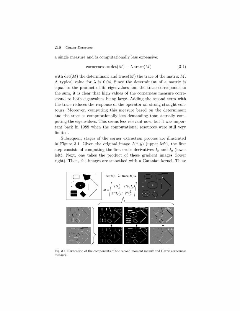
218 Corner Detectors
a single measure and is computationally less expensive:
cornerness = det(M) − λ trace(M) (3.4)
with det(M) the determinant and trace(M) the trace of the matrix M .A typical value for λ is 0.04. Since the determinant of a matrix isequal to the product of its eigenvalues and the trace corresponds tothe sum, it is clear that high values of the cornerness measure corre-spond to both eigenvalues being large. Adding the second term withthe trace reduces the response of the operator on strong straight con-tours. Moreover, computing this measure based on the determinantand the trace is computationally less demanding than actually com-puting the eigenvalues. This seems less relevant now, but it was impor-tant back in 1988 when the computational resources were still verylimited.
Subsequent stages of the corner extraction process are illustratedin Figure 3.1. Given the original image I(x,y) (upper left), the firststep consists of computing the first-order derivatives Ix and Iy (lowerleft). Next, one takes the product of these gradient images (lowerright). Then, the images are smoothed with a Gaussian kernel. These
yI 2xI 2Iy I yIx
)g*(Ix yI2g*Iyg*Ix2xI
M =g*(Ix g*I
g*(Ixg*I
y2
2x
yI )
)yI
trace(M) =λdet(M) −
Fig. 3.1 Illustration of the components of the second moment matrix and Harris cornernessmeasure.

3.2 Harris Detector 219
images contain the different elements of the Hessian matrix, which arethen in a final step combined into the cornerness measure, followingEquation (3.4) (upper right).
When used as an interest point detector, local maxima of the cor-nerness function are extracted, using non-maximum suppression. Suchpoints are translation and rotation invariant. Moreover, they are stableunder varying lighting conditions. In a comparative study of differ-ent interest point detectors [214, 215], the Harris corner was provento be the most repeatable and most informative. Additionally, theycan be made very precise: sub-pixel precision can be achieved throughquadratic approximation of the cornerness function in the neighbor-hood of a local maximum.
3.2.1 Discussion
Figure 3.2 shows the corners detected with this measure for two exam-ple images related by a rotation. Note that the features found corre-spond to locations in the image showing two dimensional variations inthe intensity pattern. These may correspond to real “corners”, but thedetector also fires on other structures, such as T-junctions, points withhigh curvature, etc. This equally holds for all other corner detectorsdescribed in this chapter. When true corners are desirable, model-basedapproaches are certainly more appropriate.
Fig. 3.2 Harris corners detected on rotated image examples.

220 Corner Detectors
As can be seen in the figure, many but not all of the featuresdetected in the original image (left) have also been found in the rotatedversion (right). In other words, the repeatability of the Harris detectorunder rotations is high.
Additionally, features are typically found at locations which areinformative, i.e., with a high variability in the intensity pattern.This makes them more discriminative and easier to bring intocorrespondence.
3.3 SUSAN Detector
The SUSAN corner detector has been introduced by Smith andBrady [232] and relies on a different technique. Rather than evaluat-ing local gradients, which might be noise-sensitive and computationallymore expensive, a morphological approach is used.
SUSAN stands for Smallest Univalue Segment AssimilatingNucleus, and is a generic low-level image processing technique, whichapart from corner detection has also been used for edge detectionand noise suppression. The basic principle goes as follows (see alsoFigure 3.3). For each pixel in the image, we consider a circular neigh-borhood of fixed radius around it. The center pixel is referred to asthe nucleus, and its intensity value is used as reference. Then, all other
Fig. 3.3 SUSAN corners are detected by segmenting a circular neighborhood into “similar”(orange) and “dissimilar” (blue) regions. Corners are located where the relative area of the“similar” region (usan) reaches a local minimum below a certain threshold.
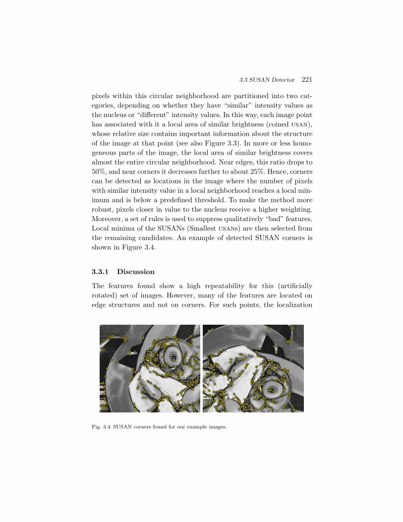
3.3 SUSAN Detector 221
pixels within this circular neighborhood are partitioned into two cat-egories, depending on whether they have “similar” intensity values asthe nucleus or “different” intensity values. In this way, each image pointhas associated with it a local area of similar brightness (coined usan),whose relative size contains important information about the structureof the image at that point (see also Figure 3.3). In more or less homo-geneous parts of the image, the local area of similar brightness coversalmost the entire circular neighborhood. Near edges, this ratio drops to50%, and near corners it decreases further to about 25%. Hence, cornerscan be detected as locations in the image where the number of pixelswith similar intensity value in a local neighborhood reaches a local min-imum and is below a predefined threshold. To make the method morerobust, pixels closer in value to the nucleus receive a higher weighting.Moreover, a set of rules is used to suppress qualitatively “bad” features.Local minima of the SUSANs (Smallest usans) are then selected fromthe remaining candidates. An example of detected SUSAN corners isshown in Figure 3.4.
3.3.1 Discussion
The features found show a high repeatability for this (artificiallyrotated) set of images. However, many of the features are located onedge structures and not on corners. For such points, the localization
Fig. 3.4 SUSAN corners found for our example images.

222 Corner Detectors
is sensitive to noise. Moreover, edge based points are also lessdiscriminative.
The two detectors described so far are invariant under translationand rotation only. This means that corners will be detected at cor-responding locations only if the images are related by a translationand/or rotation. In the next sections, we will describe detectors withhigher levels of viewpoint invariance, that can withstand scale changesor even affine deformations. Apart from better matching across trans-formed images, these also bring the advantage of detecting features overa range of scales or shapes.
Alternatively, this effect can be obtained by using a multiscaleapproach. In that case, a detector which is not scale invariant isapplied to the input image at different scales (i.e., after smoothingand sampling).
3.4 Harris-Laplace/Affine
Mikolajczyk and Schmid developed both a scale invariant corner detec-tor, referred to as Harris-Laplace, as well as an affine-invariant one,referred to as Harris-Affine [143].
3.4.1 Harris-Laplace
Harris-Laplace starts with a multiscale Harris corner detector as ini-tialization to determine the location of the local features. The charac-teristic scale is then determined based on scale selection as proposed byLindeberg et al. [116, 120]. The idea is to select the characteristic scaleof a local structure, for which a given function attains an extremum overscales (see Figure 3.5). The selected scale is characteristic in the quan-titative sense, since it measures the scale at which there is maximumsimilarity between the feature detection operator and the local imagestructures. The size of the region is therefore selected independently ofthe image resolution for each point. As the name Harris-Laplace sug-gests, the Laplacian operator is used for scale selection. This has beenshown to give the best results in the experimental comparison of [141]as well as in [38]. These results can be explained by the circular shape

3.4 Harris-Laplace/Affine 223
Fig. 3.5 Example of characteristic scales. The top row shows images taken with differentzoom. The bottom row shows the responses of the Laplacian over scales for two corre-sponding points. The characteristic scales are 10.1 and 3.9 for the left and right images,respectively. The ratio of scales corresponds to the scale factor (2.5) between the two images.The radius of displayed regions in the top row is equal to 3 times the selected scales.
of the Laplacian kernel, which acts as a matched filter [58] when itsscale is adapted to the scale of a local image structure.
Figure 3.6 shows the scale-invariant local features obtained byapplying the Harris-Laplace detector, for two images of the same scenerelated by a scale change. In order not to overload the images, onlysome of the corresponding regions that were detected in both images
Fig. 3.6 Corresponding features found with the Harris-Laplace detector. Only a subset ofcorresponding features is displayed to avoid clutter. The circles indicate the scale of thefeatures.

224 Corner Detectors
are shown. A similar selection mechanism has been used for all subse-quent image pairs shown in this survey.
3.4.2 Harris-Affine
Given a set of initial points extracted at their characteristic scalesbased on the Harris-Laplace detection scheme, the iterative estimationof elliptical affine regions as proposed by Lindeberg et al. [118, 121]allows to obtain affine invariant corners. Instead of circular regions,these are ellipses. The procedure consists of the following steps:
(1) Detect the initial region with the Harris-Laplace detector.(2) Estimate the affine shape with the second moment matrix.(3) Normalize the affine region to a circular one.(4) Re-detect the new location and scale in the normalized
image.(5) Go to step 2 if the eigenvalues of the second moment matrix
for the new point are not equal.
The iterations are illustrated in Figure 3.7.
Fig. 3.7 Iterative detection of an affine invariant interest point in the presence of an affinetransformation (top and bottom rows). The first column shows the points used for initial-ization. The consecutive columns show the points and regions after iterations 1, 2, 3, and 4.Note that the regions converge after 4 iterations to corresponding image regions.

3.4 Harris-Laplace/Affine 225
Fig. 3.8 Diagram illustrating the affine normalization using the second moment matrices.Image coordinates are transformed with matrices M
−1/2L and M
−1/2R .
The eigenvalues of the second moment matrix (see Equation (3.3))are used to measure the affine shape of the point neighborhood. Moreprecisely, we determine the transformation that projects the intensitypattern of the point neighborhood to one with equal eigenvalues. Thistransformation is given by the square root of the second moment matrixM1/2. It can be shown that if the neighborhoods of two points xR andxL are related by an affine transformation, then their normalized ver-sions, xR = M
−1/2R x′
R and xL = M−1/2L x′
L, are related by a simple rota-tion x′
L = Rx′R [13, 121]. This process is illustrated in Figure 3.8. The
matrices M ′L and M ′
R computed in the normalized frames are rotationmatrices as well. Note that rotation preserves the eigenvalue ratio foran image patch, therefore, the affine deformation can be determinedonly up to a rotation factor.
The estimation of affine shape can be applied to any initial pointgiven that the determinant of the second moment matrix is larger thanzero and the signal to noise ratio is sufficiently large. We can thereforeuse this technique to estimate the shape of initial regions provided bythe Harris-Laplace detector.
The output of the Harris-Affine detector on two images of the samescene is shown in Figure 3.9. Apart from the scale, also the shape ofthe regions is now adapted to the underlying intensity patterns, so as

226 Corner Detectors
Fig. 3.9 Harris-Affine regions generated for two different views of a planar scene (subset).In spite of the affine deformation, the region shapes clearly correspond.
to ensure that the same part of the object surface is covered in spite ofthe deformations caused by the viewpoint change.
3.5 Edge-based Regions
A more heuristic technique to obtain affine invariance is to exploit thegeometry of the edges that can usually be found in the proximity ofa Harris corner. Such a method has been proposed by Tuytelaars andVan Gool [247, 249]. The rationale behind this approach is that edgesare typically rather stable image features, that can be detected overa range of viewpoints, scales and illumination changes. Moreover, byexploiting the edge geometry, the dimensionality of the problem canbe significantly reduced. Indeed, as will be shown next, the 6D searchproblem over all possible affinities (or 4D, once the center point is fixed)can be reduced to a one-dimensional problem by exploiting the nearbyedges geometry. In practice, we start from a Harris corner point p (seeSection 3.2) [84] and a nearby edge, extracted with the Canny edgedetector [29]. To increase the robustness to scale changes, these basicfeatures are extracted at multiple scales. Two points p1 and p2 moveaway from the corner in both directions along the edge, as shown inFigure 3.10. Their relative speed is coupled through the equality ofrelative affine invariant parameters l1 and l2:
li =∫
abs(|pi(1)(si)p − pi(si)|)dsi (3.5)

3.5 Edge-based Regions 227
p
p
p1
2
l
l1
2
q
Fig. 3.10 The edge-based region detector starts from a corner point p and exploits nearbyedge information.
with si an arbitrary curve parameter (in both directions, i = 1,2),pi
(1)(si) the first derivative of pi(si) with respect to si, abs( ) the abso-lute value and | · · · | the determinant. This condition prescribes thatthe areas between the joint 〈p,p1〉 and the edge and between the joint〈p,p2〉 and the edge remain identical. From now on, we simply use l
when referring to l1 = l2.For each value l, the two points p1(l) and p2(l) together with the
corner p define a parallelogram Ω(l): the parallelogram spanned by thevectors p1(l) − p and p2(l) − p (see Figure 3.10). This yields a one-dimensional family of parallelogram-shaped regions as a function of l.From this 1D family one (or a few) parallelogram(s) are selected forwhich the following photometric quantities of the texture go throughan extremum.
Inv1 = abs( |p1 − pg p2 − pg|
|p − p1 p − p2|)
M100√
M200M
000 − (M1
00)2
Inv2 = abs( |p − pg q − pg|
|p − p1 p − p2|)
M100√
M200M
000 − (M1
00)2(3.6)
with
Mnpq =
∫Ω
In(x,y)xpyq dxdy
pg =(
M110
M100
,M1
01
M100
)(3.7)
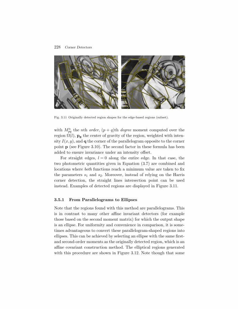
228 Corner Detectors
Fig. 3.11 Originally detected region shapes for the edge-based regions (subset).
with Mnpq the nth order, (p + q)th degree moment computed over the
region Ω(l), pg the center of gravity of the region, weighted with inten-sity I(x,y), and q the corner of the parallelogram opposite to the cornerpoint p (see Figure 3.10). The second factor in these formula has beenadded to ensure invariance under an intensity offset.
For straight edges, l = 0 along the entire edge. In that case, thetwo photometric quantities given in Equation (3.7) are combined andlocations where both functions reach a minimum value are taken to fixthe parameters s1 and s2. Moreover, instead of relying on the Harriscorner detection, the straight lines intersection point can be usedinstead. Examples of detected regions are displayed in Figure 3.11.
3.5.1 From Parallelograms to Ellipses
Note that the regions found with this method are parallelograms. Thisis in contrast to many other affine invariant detectors (for examplethose based on the second moment matrix) for which the output shapeis an ellipse. For uniformity and convenience in comparison, it is some-times advantageous to convert these parallelogram-shaped regions intoellipses. This can be achieved by selecting an ellipse with the same first-and second-order moments as the originally detected region, which is anaffine covariant construction method. The elliptical regions generatedwith this procedure are shown in Figure 3.12. Note though that some

3.6 Discussion 229
Fig. 3.12 Edge-based regions generated for the two example images, represented withellipses (subset).
information is lost during this conversion, as ellipses have a rotationaldegree of freedom, which was fixed in the original representation.
3.6 Discussion
Several methods for corner detection have been described in this chap-ter. As discussed earlier, corner based features do not necessarily cor-respond to real corners in the 3D world. Indeed, the goal is to extractstable features, that can be matched well in spite of changes in viewingconditions.
The Harris detector was identified as the most stable one in manyindependent evaluations [83, 138, 215]. There are also multi-scale aswell as scale and affine invariant extensions of this approach. It is aconvenient tool for providing a large number of features. Alternatively,the SUSAN detector can be used. It is more efficient but also moresensitive to noise. An optimized SUSAN detector using machine learn-ing techniques is described in Section 6.3. As discussed in Sections 2.2and 2.3 contour based corner detectors are suitable for line drawingimages but in natural scenes intensity based methods are typically morestable.
It is important to note that the affine transformation model onlyholds for viewpoint changes in case of locally planar regions and assum-ing the camera is relatively far from the object. However, corners areoften found near object boundaries as this is where the intensity change

230 Corner Detectors
usually occurs. Hence, the region extraction process is often based onmeasurements on non-planar structures, e.g., including background oranother facet of the object. In these cases, the viewpoint invariancewill be limited and also the robustness to background changes will beaffected. A possible way out has been indicated in the work of [251].Detectors that search for region boundaries like EBR are less affectedby this phenomenon. The measurement regions can then be delimitedby the detected contours, thus excluding the non-planar parts in manypractical situations.
On the positive side, compared to other types of features, corners aretypically better localized in the image plane. This localization accuracycan be important for some applications, e.g., for camera calibration or3D reconstruction. Their scale however is not well defined as a cornerstructure changes very little over a wide range of scales. The reason whyscale selection still works with the Harris detector is that the featurepoint is localized not exactly on the corner edge but slightly inside thecorner structure.

4Blob Detectors
After corners, the second most intuitive local features are blobs. Asit was the case in the previous section, we select a few methods thathave proved successful in many applications and describe these in moredetail. These methods typically provide complementary features to theones discussed in the previous chapter. We start with a derivative-based method: the Hessian detector (Section 4.1). Next, we consider thescale-invariant and affine invariant extensions of this method, coinedHessian-Laplace and Hessian-Affine (Section 4.2). Finally, we describethe salient region detector, which is based on the entropy of the inten-sity probability distribution (Section 4.3). We conclude the chapter witha short discussion.
4.1 Hessian Detector
The second 2 × 2 matrix issued from the Taylor expansion of the imageintensity function I(x) is the Hessian matrix:
H =[Ixx(x,σD) Ixy(x,σD)Ixy(x,σD) Iyy(x,σD)
](4.1)
with Ixx etc. second-order Gaussian smoothed image derivatives. Theseencode the shape information by describing how the normal to an
231

232 Blob Detectors
isosurface changes. As such, they capture important properties of localimage structure. Particularly interesting are the filters based on thedeterminant and the trace of this matrix. The latter is often referredto as the Laplacian. Local maxima of both measures can be used todetect blob-like structures in an image [16].
The Laplacian is a separable linear filter and can be approximatedefficiently with a Difference of Gaussians (DoG) filter. The Lapla-cian filters have one major drawback in the context of blob extrac-tion though. Local maxima are often found near contours or straightedges, where the signal change is only in one direction [138]. Thesemaxima are less stable because their localization is more sensitiveto noise or small changes in neighboring texture. This is mostly anissue in the context of finding correspondences for recovering imagetransformations. A more sophisticated approach, solving this prob-lem, is to select a location and scale for which the trace and thedeterminant of the Hessian matrix simultaneously assume a localextremum.
This gives rise to points, for which the second order derivativesdetect signal changes in two orthogonal directions. A similar idea isexplored in the Harris detector, albeit for first-order derivatives only.
The feature detection process based on the Hessian matrix is illus-trated in Figure 4.1. Given the original image (upper left), one firstcomputes the second-order Gaussian smoothed image derivatives (lowerpart), which are then combined into the determinant of the Hessian(upper right).
The interest points detected with the determinant of the Hessian foran example image pair are displayed in Figure 4.2. The second-orderderivatives are symmetric filters, thus they give weak responses exactlyin the point where the signal change is most significant. Therefore,the maxima are localized at ridges and blobs for which the size of theGaussian kernel σD matches by the size of the blob structure.
4.2 Hessian-Laplace/Affine
The Hessian-Laplace and Hessian-Affine detectors are similar in spiritas their Harris-based counterparts Harris-Laplace and Harris-Affine,

4.2 Hessian-Laplace/Affine 233
I yyxxI I xy
− III =2xyyyxx
Fig. 4.1 Illustration of the components of the Hessian matrix and Hessian determinant.
Fig. 4.2 Output of the Hessian detector applied at a given scale to example images withrotation (subset).
described in Section 3.4, except that they start from the determinant ofthe Hessian rather than the Harris corners. This turns the methods intoviewpoint invariant blob-detectors. They have also been proposed byMikolajczyk and Schmid [143], and are complementary to their Harris-based counterparts, in the sense that they respond to a different typeof feature in the image. An example of the detection result is shown inFigures 4.3 and 4.4 for the scale-invariant Hessian-Laplace and affineinvariant Hessian-Affine, respectively.

234 Blob Detectors
Fig. 4.3 Output of Hessian-Laplace detector applied to example images with scale change(subset).
Fig. 4.4 Hessian-Affine regions generated for two views of the example scene (subset).
Like in the Harris based detector the number of regions found withthe Hessian-Laplace detector can be controlled by thresholding theHessian determinant as well as the Laplacian response. Typically alarge number of features can be extracted resulting in a good cover-age of the image, which is one of the advantages of the Hessian-baseddetector.
Furthermore, this detector also responds to some corner structuresat fine scale (see Figure 4.1). The returned locations, however, are moresuitable for scale estimation than the Harris points due to the use ofsimilar filters for spatial and scale localization, both based on second-order Gaussian derivatives. One of the possible extensions of this work

4.3 Salient Regions 235
is to explore the Hessian matrix to use additional shape informationencoded by the eigenvalues of this matrix.
4.3 Salient Regions
Rather than building on the derivative information in the image, thesalient region detector proposed by Kadir and Brady [98] is inspiredby information theory. The basic idea behind this feature detector is tolook for salient features, where saliency is defined as local complexityor unpredictability. It is measured by the entropy of the probability dis-tribution function of intensity values within a local image region. How-ever, looking at entropy alone does not suffice to accurately localize thefeatures over scales, so as an additional criterion, the self-dissimilarityin scale-space of the feature is added as an extra weighting function,favoring well-localized complex features.
Detection proceeds in two steps: first, at each pixel x the entropy Hof the probability distribution p(I) is evaluated over a range of scales s.
H = −∑
I
p(I) logp(I).
The probability distribution p(I) is estimated empirically based onthe intensity distribution in a circular neighbourhood of radius s
around x. Local maxima of the entropy are recorded. These are candi-date salient regions. Second, for each of the candidate salient regionsthe magnitude of the derivative of p(I) with respect to scale s iscomputed as
W =s2
2s − 1
∑I
∣∣∣∣∂p(I;s)∂s
∣∣∣∣ .The saliency Y is then computed as
Y = WH.
The candidate salient regions over the entire image are ranked by theirsaliency Y, and the top P ranked regions are retained.
Also an affine invariant version of the detector has been proposed,where local maxima over the scale s and the shape parameters (orien-tation θ and ratio of major to minor axes λ of an elliptical region)

236 Blob Detectors
Fig. 4.5 Salient regions found for the two example images related to a change in viewpoint(subset).
are sought simultaneously. However, this seriously slows down thecomputation.
Examples of detected regions, using the affine invariant version, aredisplayed in Figure 4.5. More details about this method can be foundin [99].
4.3.1 Discussion
Because of the weighting factor measuring the self-dissimilarity overscale, the detector typically fires on blob-like structures in the image.That is why we have catalogued the method as a blob detector. Butnote that in contrast to other blob detectors the contrast of the blobsdoes not have any influence on the detection.
The number of features found with this method is typically rela-tively low. Unlike for many other detectors the ranking of the extractedfeatures is meaningful due to the entropy based criteria with the onesfrom the top the most stable. This property has been explored in thecontext of category-level object recognition, and especially in combi-nation with classifiers where the complexity largely depends on thenumber of features (e.g., [65]).
4.4 Discussion
Blob detectors have been used widely in different application domains.Apart from the methods described above, also DoG (difference-of-

4.4 Discussion 237
Gaussians) [124] and SURF (speeded-up robust features) [15] can becatalogued as blob detectors. However, since their extraction processesare focussed on efficiency, we postpone their discussion until Section 6.
Some of the methods described in Section 5 also share commoncharacteristics with blob detectors. Especially IBR (intensity-basedregions) [248] and MSER (maximally stable extremal regions) [134]often find blob-like structures in the image. However, apart from blob-like structures, they also detect other, more irregularly shaped patterns,which we consider their distinctive property.
Blob detectors are in a sense complementary to corner detectors.As a result, they are often used together. By using several complemen-tary feature detectors, the image is better covered and the performancebecomes less dependent on the actual image content. This has beenexploited, e.g., in [110, 140, 231].
In general, blob-like structures tend to be less accurately localizedin the image plane than corners, although their scale and shape are bet-ter defined than for corners. The location of a corner can be identifiedby a single point while blobs can only be localized by their boundaries,which are often irregular. On the other hand, the scale estimation of acorner is ill-defined as for example an intersection of edges exists at awide range of scales. The boundaries of a blob however, even if irregu-lar, give a good estimate of the size thus scale of the blob. This makesthem less suited for, e.g., camera calibration or 3D reconstruction. Forobject recognition, on the other hand, a precise image localization isoften not necessary, since the entire recognition process is very noisy.A robust descriptor such as SIFT [124] can match such features nev-ertheless. The scales of matched blobs allow then to hypothesize thesize of the objects [140], which makes them very useful in recognitionapplications.
Finally, the number of features detected with the methods describedabove varies greatly. There is often just a few tens of salient regionsfound in an image, whereas the Hessian-Laplace or Hessian-Affinemethods allow to extract up to several hundreds or thousands of fea-tures. Depending on the application and algorithms used, either casecan be advantageous. We refer to Section 7 for a further discussion onthis issue.

5Region Detectors
In this chapter, we discuss a number of feature detectors which, directlyor indirectly, are concerned with extraction of image regions. First, wedescribe the intensity-based regions (Section 5.1), followed by maximallystable extremal regions (Section 5.2). At the end, we discuss superpix-els (Section 5.3). These regions are provided by different methods butfocus on similar image structures and share similar properties. Super-pixels are traditionally not considered as local features and have limitedrobustness to changes in viewing conditions but they are currently moreand more used in the context of image recognition. We therefore includeall the above features in the same category.
5.1 Intensity-based Regions
Here we describe a method proposed by Tuytelaars and Van Gool [248,249] to detect affine invariant regions. It starts from intensity extrema(detected at multiple scales), and explores the image around them ina radial way, delineating regions of arbitrary shape, which are thenreplaced by ellipses.
More precisely, given a local extremum in intensity, the intensityfunction along rays emanating from the extremum is studied (see
238
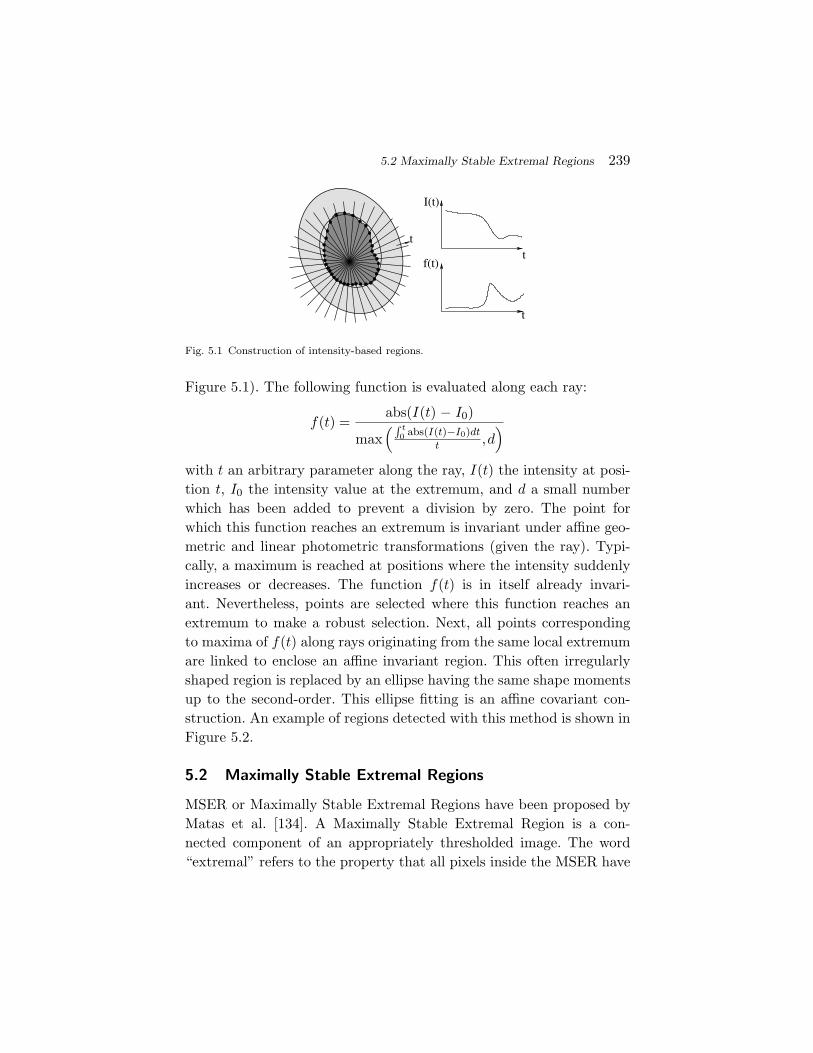
5.2 Maximally Stable Extremal Regions 239
I(t)
f(t)
t
tt
Fig. 5.1 Construction of intensity-based regions.
Figure 5.1). The following function is evaluated along each ray:
f(t) =abs(I(t) − I0)
max(∫ t
0 abs(I(t)−I0)dt
t ,d)
with t an arbitrary parameter along the ray, I(t) the intensity at posi-tion t, I0 the intensity value at the extremum, and d a small numberwhich has been added to prevent a division by zero. The point forwhich this function reaches an extremum is invariant under affine geo-metric and linear photometric transformations (given the ray). Typi-cally, a maximum is reached at positions where the intensity suddenlyincreases or decreases. The function f(t) is in itself already invari-ant. Nevertheless, points are selected where this function reaches anextremum to make a robust selection. Next, all points correspondingto maxima of f(t) along rays originating from the same local extremumare linked to enclose an affine invariant region. This often irregularlyshaped region is replaced by an ellipse having the same shape momentsup to the second-order. This ellipse fitting is an affine covariant con-struction. An example of regions detected with this method is shown inFigure 5.2.
5.2 Maximally Stable Extremal Regions
MSER or Maximally Stable Extremal Regions have been proposed byMatas et al. [134]. A Maximally Stable Extremal Region is a con-nected component of an appropriately thresholded image. The word“extremal” refers to the property that all pixels inside the MSER have
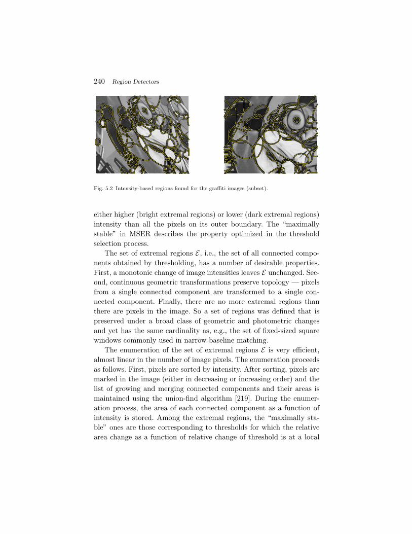
240 Region Detectors
Fig. 5.2 Intensity-based regions found for the graffiti images (subset).
either higher (bright extremal regions) or lower (dark extremal regions)intensity than all the pixels on its outer boundary. The “maximallystable” in MSER describes the property optimized in the thresholdselection process.
The set of extremal regions E , i.e., the set of all connected compo-nents obtained by thresholding, has a number of desirable properties.First, a monotonic change of image intensities leaves E unchanged. Sec-ond, continuous geometric transformations preserve topology — pixelsfrom a single connected component are transformed to a single con-nected component. Finally, there are no more extremal regions thanthere are pixels in the image. So a set of regions was defined that ispreserved under a broad class of geometric and photometric changesand yet has the same cardinality as, e.g., the set of fixed-sized squarewindows commonly used in narrow-baseline matching.
The enumeration of the set of extremal regions E is very efficient,almost linear in the number of image pixels. The enumeration proceedsas follows. First, pixels are sorted by intensity. After sorting, pixels aremarked in the image (either in decreasing or increasing order) and thelist of growing and merging connected components and their areas ismaintained using the union-find algorithm [219]. During the enumer-ation process, the area of each connected component as a function ofintensity is stored. Among the extremal regions, the “maximally sta-ble” ones are those corresponding to thresholds for which the relativearea change as a function of relative change of threshold is at a local

5.2 Maximally Stable Extremal Regions 241
minimum. In other words, the MSER are the parts of the image wherelocal binarization is stable over a large range of thresholds. The defi-nition of MSER stability based on relative area change is invariant toaffine transformations (both photometrically and geometrically).
Detection of MSER is related to thresholding, since every extremalregion is a connected component of a thresholded image. However, noglobal or “optimal” threshold is sought, all thresholds are tested andthe stability of the connected components evaluated. The output ofthe MSER detector is not a binarized image. For some parts of theimage, multiple stable thresholds exist and a system of nested subsetsis output in this case.
For many of the affine invariant detectors the output shape is anellipse. However, for MSER it is not. Examples of the original regionsdetected are given in Figure 5.3. Using the same procedure as explainedabove for the IBR, an ellipse can be fitted based on the first and secondshape moments. This results in a set of features as shown in Figure 5.4.Alternatively, a local affine frame can be defined based on a set of sta-ble points along the region contour [135]. This provides an alternativescheme to normalize the region against affine deformations.
5.2.1 Discussion
The MSER features typically anchor on region boundaries, thusthe resulting regions are accurately localized compared to other
Fig. 5.3 Regions detected with MSER on the graffiti images (subset).

242 Region Detectors
Fig. 5.4 Final MSER regions for the graffiti images (subset).
blob-detectors. The method works best for structured images which canbe segmented well — ideally an image with uniform regions separatedby strong intensity changes. On the downside, it was found to be sensi-tive to image blur [145], which can be explained by the fact that imageblur undermines the stability criterion. This issue was addressed in itsrecent extension in [177]. The method is also relatively fast. It is cur-rently the most efficient among the affine invariant feature detectors.It has been used mostly for recognizing or matching specific objects(e.g., [166, 231]) and showed lower performance for object class recog-nition [139].
5.3 Segmentation-based Methods (Superpixels)
The two methods described above extract small regions whose intensitypatterns clearly stand out with respect to their immediate surround-ings. This is reminiscent of traditional image segmentation techniques.However, image segments are typically relatively large — too large, infact, to be used as local features. By increasing the number of segmentsa new image representation can be obtained where the image segmentstypically have the right trade-off between locality and distinctivenessrequired in most local features-based applications (see Figure 5.5). Thislow-level grouping of pixels into atomic regions has been advocated byMori et al. [159] and Ren and Malik [184], who refer to the resultingatomic regions as superpixels. This terminology refers to the fact that

5.3 Segmentation-based Methods (Superpixels) 243
Fig. 5.5 Superpixels generated for the example image.
superpixels can be considered as a more natural and perceptually moremeaningful alternative for the original image pixels.
In [159, 184], superpixels are extracted from the image using nor-malized cuts [227], but any data driven segmentation methods can beused here. The normalized cuts based approach is a classical imagesegmentation algorithm which exploits pairwise brightness, color, ortexture affinities between pixels. To enforce locality, only local connec-tions are taken into account when constructing the affinity matrix. Anexample of superpixels is shown in Figure 5.5.
In contrast to traditional local features, by construction superpixelscover the entire image and do not overlap. Multiple segmentations canalso be used to increase the possibility of object boundaries coincidingwith boundaries between adjacent superpixels, except for small contourdetails and invisible contours. All superpixels extracted from an imagehave similar scale, so the method is not scale-invariant. An alternativeconstruction method, based on Constrained Delauney Triangulation,has been proposed to obtain robustness against scale change [183].
These features are less suited for matching or object recognition, asthe regions are uniform therefore not discriminative and the repeata-bility of boundary extraction is low. They have been used successfullyfor modeling and exploiting mid-level visual cues, such as curvilinearcontinuity, region grouping, or figure/ground organization for semanticimage segmentation.

244 Region Detectors
5.4 Discussion
The local features detected with the methods described above typi-cally represent homogeneous regions. While this is acceptable for thedetection step, it may incur problems for the later description andmatching. Indeed, homogeneous regions lack distinctiveness. Fortu-nately, this can easily be overcome by increasing the measurementregion. In other words, we use a larger scale region to compute thedescriptor, such that it also contains part of the surrounding imagestructures and captures the shape of the region boundary. This usuallysuffices to increase the discriminative power and match regions betweenimages.
Intensity-based regions and maximally stable extremal regions typ-ically give very similar features. These methods are therefore not com-plementary. IBR may break down when the region is non-convex, butit is more robust to small gaps in the region contour. MSER, on theother hand, has been shown to be relatively sensitive to image blurin [145], as this directly affects the stability criterion. This problem hasbeen recently addressed in [177]. However, apart from the case of imageblur, MSER scores best with respect to repeatability in [145].
As discussed earlier, region detectors often detect blob-like struc-tures — although they are not restricted to this type of regions. As aresult, they are less complementary to blobs then to corners.
Region-based detectors are typically quite accurate in their local-ization. They work especially well for images with a well structuredscene, clearly delineated regions, such as images containing objects withprinted surfaces, buildings etc.
Even though superpixels share some characteristics with the otherregion detectors, they are not the same. They are non-overlapping,and cover the entire image. Their repeatability suffers from the weakrobustness of the segmentation methods. Most importantly, they havebeen developed in a different context, where the idea is to speed upthe image analysis by focussing on the superpixels only instead of ana-lyzing all pixels. Superpixels are hence considered as a bigger equiv-alent of pixels, which can be described to a first approximation by

5.4 Discussion 245
a single intensity or color value. This is in contrast to local featureswhich should be distinctive and, in the ideal case, uniquely identifiable.However, using region boundaries to build distinctive descriptors mayovercome the occlusion problem from which traditional interest pointssuffer [68].

6Efficient Implementations
Most feature detectors described so far involve the computation ofderivatives or more complex measures such as the second momentmatrix for the Harris detector or entropy for the salient regions detec-tor. Since this step needs to be repeated for each and every location infeature coordinate space which includes position, scale and shape, thismakes the feature extraction process computationally expensive, thusnot suitable for many applications.
In this section we describe several feature detectors that have beendeveloped with computational efficiency as one of the main objectives.The DoGs detector approximates the Laplacian using multiple scale-space pyramids (see Section 6.1). SURF makes use of integral imagesto efficiently compute a rough approximation of the Hessian matrix(Section 6.2). FAST evaluates only a limited number of individual pixelintensities using decision trees (see Section 6.3).
6.1 Difference-of-Gaussians
The Difference-of-Gaussians detector, or DoG for short, has been pro-posed in [47, 76, 81, 124, 126]. It is a scale-invariant detector which
246

6.1 Difference-of-Gaussians 247
extracts blobs in the image by approximating the Laplacian L2xx + L2
yy
(see also Section 4.1). Based on the diffusion equation in scale-spacetheory [117, 234, 258], it can be shown that the Laplacian correspondsto the derivative of the image in the scale direction. Since the differ-ence between neighboring points in a given direction approximates thederivative in this direction, the difference between images at differentscales approximates the derivative with respect to scale. Furthermore,Gaussian blurring is often applied to generate images at various scales.Hence, the DoG images produce responses which approximate the LoG.The computation of second-order derivatives in x and y directions isthen avoided, as illustrated in Figure 6.1.
The actual computation scheme is illustrated in Figure 6.2. Theimage is smoothed several times with a Gaussian convolution mask.These smoothed versions are combined pairwise to compute a set ofDoG blob response maps. Local maxima in these maps are locatedboth over space and over scales with non-maximal suppression, andthe locations are further refined with quadratic interpolation. After afew smoothing steps, the image can be subsampled to process the nextoctave.
Since the Laplacian gives strong response on edges, an additionalfiltering step is added, where the eigenvalues of the full Hessian matrixare computed and their strengths evaluated. This filtering step doesnot affect the overall processing time too much, as it is only neededfor a limited number of image locations and scales. The DoG featuresdetected in our example images are shown in Figure 6.3. Several framesper second can be processed with this method.
Fig. 6.1 The Laplacian can be approximated as a difference of two Gaussian smoothedimages.

248 Efficient Implementations
Fig. 6.2 Overview of the DoG-detection scheme.
Fig. 6.3 Local features detected with the DoG-detector.
6.2 SURF: Speeded Up Robust Features
In the context of realtime face detection, Viola and Jones have proposedto use integral images [252], which allow for very fast computation ofHaar wavelets or any box-type convolution filter. First, we will describethe basic idea of integral images. Then we show how this technique canbe used to obtain a fast approximation of the Hessian matrix, as usedin SURF (Speeded-Up Robust Features) [15].
6.2.1 Integral Images
The entry of an integral image IΣ(x) at a location x = (x, y) representsthe sum of all pixels in the input image I of a rectangular region formed

6.2 SURF: Speeded Up Robust Features 249
Fig. 6.4 Using integral images, it takes only four operations to calculate the area of arectangular region of any size.
by the origin and x.
IΣ(x) =i≤x∑i=0
j≤y∑j=0
I(i, j). (6.1)
Once the integral image has been computed, it takes four additionsto calculate the sum of the intensities over any upright, rectangulararea, as shown in Figure 6.4. Moreover, the calculation time is inde-pendent of the size of the rectangular area.
6.2.2 SURF
SURF or Speeded Up Robust Features have been proposed by Bayet al. [15, 14]. It is a scale-invariant feature detector based on theHessian-matrix, as is, e.g., the Hessian-Laplace detector (see Sec-tion 4.2). However, rather than using a different measure for selectingthe location and the scale, the determinant of the Hessian is used forboth. The Hessian matrix is roughly approximated, using a set of box-type filters, and no smoothing is applied when going from one scale tothe next.
Gaussians are optimal for scale-space analysis [7, 67, 106, 117], butin practice they have to be discretized (Figure 6.5 left) which introducesartifacts, in particular in small Gaussian Kernels. SURF pushes theapproximation even further, using the box filters as shown in the right
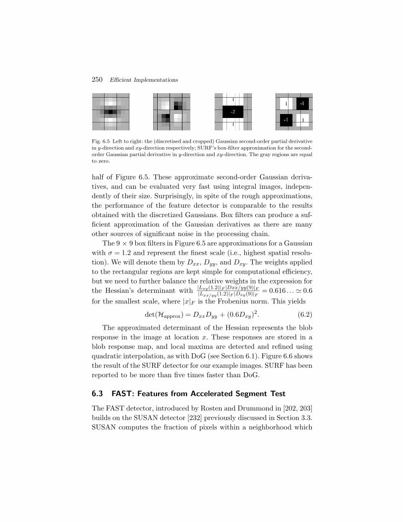
250 Efficient Implementations
Fig. 6.5 Left to right: the (discretised and cropped) Gaussian second-order partial derivativein y-direction and xy-direction respectively; SURF’s box-filter approximation for the second-order Gaussian partial derivative in y-direction and xy-direction. The gray regions are equalto zero.
half of Figure 6.5. These approximate second-order Gaussian deriva-tives, and can be evaluated very fast using integral images, indepen-dently of their size. Surprisingly, in spite of the rough approximations,the performance of the feature detector is comparable to the resultsobtained with the discretized Gaussians. Box filters can produce a suf-ficient approximation of the Gaussian derivatives as there are manyother sources of significant noise in the processing chain.
The 9 × 9 box filters in Figure 6.5 are approximations for a Gaussianwith σ = 1.2 and represent the finest scale (i.e., highest spatial resolu-tion). We will denote them by Dxx, Dyy, and Dxy. The weights appliedto the rectangular regions are kept simple for computational efficiency,but we need to further balance the relative weights in the expression forthe Hessian’s determinant with |Lxy(1.2)|F |Dxx/yy(9)|F
|Lxx/yy(1.2)|F |Dxy(9)|F = 0.616 . . . 0.6for the smallest scale, where |x|F is the Frobenius norm. This yields
det(Happrox) = DxxDyy + (0.6Dxy)2. (6.2)
The approximated determinant of the Hessian represents the blobresponse in the image at location x. These responses are stored in ablob response map, and local maxima are detected and refined usingquadratic interpolation, as with DoG (see Section 6.1). Figure 6.6 showsthe result of the SURF detector for our example images. SURF has beenreported to be more than five times faster than DoG.
6.3 FAST: Features from Accelerated Segment Test
The FAST detector, introduced by Rosten and Drummond in [202, 203]builds on the SUSAN detector [232] previously discussed in Section 3.3.SUSAN computes the fraction of pixels within a neighborhood which

6.3 FAST: Features from Accelerated Segment Test 251
Fig. 6.6 Local features detected with the SURF-detector.
have similar intensity to the center pixel. This idea is taken further byFAST, which compares pixels only on a circle of fixed radius aroundthe point. The test criterion operates by considering a circle of 16 pix-els around the corner candidate (see Figure 6.7). Initially pixels 1 and2 are compared with a threshold, then 3 and 4 as well as the remain-ing ones at the end. The pixels are classified into dark, similar, andbrighter subsets. The ID3 algorithm from [178] is used to select thepixels which yield the most information about whether the candidatepixel is a corner. This is measured by the entropy of the positive and
2
4 3
1
Fig. 6.7 Illustration of pixels examined by the FAST detector.

252 Efficient Implementations
Fig. 6.8 Local features detected with the FAST detector.
negative corner classification responses based on this pixel. The pro-cess is applied recursively on all three subsets and terminates whenthe entropy of a subset is zero. The decision tree resulting from thispartitioning is then converted into C-code, creating a long string ofnested if-then-else statements which is compiled and used as a cornerdetector. Finally non-maxima suppression is applied on the sum of theabsolute difference between the pixels in the circle and the center pixel.This results in a very efficient detector which is up to 30 times fasterthan the DoG detector discussed in Section 6.1 — albeit not invariantto scale changes. The FAST features found in our example images aredisplayed in Figure 6.8.
An extension to a multi-scale detector by scale selection with theLaplacian function was proposed in [112]. They estimate the Laplacianusing gray-level differences between pixels on the circle and the centralone and retain only the locations where this estimate is largest. Thisproves to be sufficient to produce a large number of keypoint candidatesfrom which the unstable ones are filtered out during the recognitionprocess.
6.4 Discussion
The ultimate goal of methods focussing on efficiency is often realtimeprocessing of a video stream or dealing with large amounts of data.

6.4 Discussion 253
However, to some extent, this is a moving target. Computation powerincreases rapidly over time but so does the number of features weextract or the size of the databases we deal with. Moreover, featuredetection is not the final goal, but just the first step in a processingchain, followed by matching, tracking, object recognition, etc. In manyapplications significant performance improvement can be obtained justby increasing the number of training examples. Efficiency is thereforeone of the major properties equally important to invariance or robust-ness which should be considered when designing or selecting a featuredetector.
Coming back to the first point, especially the advent of powerfulgraphical processing units opens up new possibilities. Apart from themethods described above, which obtain a speedup by platform indepen-dent algorithmic changes, further speedups become possible by exploit-ing the special structure and parallelism that can be realized withGPUs. Some examples of such work can be found in [89, 230]. AnFPGA-based implementation of the Harris-Affine feature detector (seeSection 3.4) is discussed in [28] and of the DoG detector (see Section 6.1in [216]. This significantly reduces the time needed to compute all fea-tures on a normal-sized image and enables video frame rate processing.In spite of this new trend, the basic ideas and methods described in thissection still hold, as they are sufficiently general and widely applicable.
Finally, more efficient methods usually come at a price. A trade-off has to be made between efficiency on the one hand and accuracyor repeatability on the other hand. Surprisingly, the DoG, SURF, andFAST detectors are competitive with the standard, more computation-ally expensive feature detectors and may produce better results forsome applications.

7Discussion and Conclusion
In this final section of our survey, we give an overview of the pre-viously discussed methods and highlight their respective strengths andweaknesses. We give some hints on how to use these features, and onhow to select the appropriate feature detector for a given application.Finally, we discuss some open issues and future research directions.
7.1 How to Select Your Feature Detector?
Below, we give a few guidelines on what feature detector to use for agiven application. This does not give a precise and definitive answer,but indicates a few points one needs to consider when searching for asuitable detector. We refer the reader to Section 1.4 where we definethe properties of local features often mentioned here.
First, we organized the feature detectors in this survey based onthe type of image structures they extract — corners, blobs or regions.Depending on the image content, some of these image structures aremore common than others, thus the number of features found with agiven detector may vary for different image categories. If little is knownabout the image content in advance, it is generally recommended to
254

7.1 How to Select Your Feature Detector? 255
combine different complementary detectors, i.e., extracting differenttypes of features.
Second, feature detectors can be distinguished based on the levelof invariance. There have been many evaluations which focus on thisproperty [145, 157, 215]. One might be tempted to always select thehighest level of invariance available, so as to compensate for as muchvariability as possible. However, the discriminative power of featuresis reduced at increased levels of invariance. As more patterns are tobe judged equivalent, there is more parameters to estimate, thus morepossible sources of noise. Also, the feature detection process becomesmore complex, which affects both the computational complexity as wellas the repeatability. As a result, a basic rule of thumb is to use no moreinvariance than what is truly needed by the application at hand. More-over, if the expected transformations are relatively small, it is oftenbetter to count on the robustness of the feature detection and descrip-tion rather than to increase the level of invariance. That is also thereason why feature detectors invariant to perspective transformationsare of little use.
All detectors discussed in this survey are invariant to translationsand rotations. The former automatically follows from the use of localfeatures. The latter can be achieved relatively easily at limited extracost. Sometimes, rotation invariance is not required — e.g., if all imagesare taken upright and the objects are always upright as well (buildings,cars, etc.). In these cases, the rotation invariant detectors can be com-bined with a rotation variant descriptor, to ensure good discriminativepower. In all other cases, a descriptor with at most the same level ofinvariance as the detector is preferred.
Finally, there are a number of qualitative properties of the detec-tors to consider. Depending on the application scenario, some of theseproperties are more crucial than others. When dealing with category-level object recognition, robustness to small appearance variations isimportant to deal with the within-class variability. When fitting a para-metric model to the data, as for camera calibration or 3D modeling,the localization accuracy is essential. For online applications or appli-cations where a large amount of data needs to be processed, efficiencyis the most important criterion.

256 Discussion and Conclusion
7.2 Summary on the Detectors
Table 7.1 gives an overview of the most important properties for thefeature detectors described in Sections 3–6.
The feature detectors in Table 7.1 are organized in 4 groups accord-ing to their invariance: rotation, similarity, affine, and perspective.We compare the properties within each group. For rotation invariantfeatures the highest repeatability and localization accuracy in manytests has been obtained by the Harris detector. The Hessian detectorfinds blobs which are not as well localized and requires second-orderderivatives to be computed. The SUSAN detector avoids computationof derivatives and is known for its efficiency, however the absence ofsmoothing makes it more susceptible to noise. All the rotation invariantmethods are suitable for applications where only the spatial locationof the features is used and no large scale changes are expected, e.g.,structure from motion or camera calibration.
In the scale-invariant group Harris-Laplace shows high repeatabil-ity and localization accuracy inherited from the Harris detector [215].However, its scale estimation is less accurate due to the multiscalenature of corners. Hessian-Laplace is more robust than its single scaleversion [145]. This is due to the fact that blob-like structures are bet-ter localized in scale than corners and the detector benefits from mul-tiscale analysis although it is less accurately localized in the imageplane. DoG and SURF detectors were designed for efficiency and theother properties are slightly compromised. However, for most applica-tions they are still more than sufficient. Quantity and good coverageof the image are crucial in recognition applications, where localizationaccuracy is less important. Thus, Hessian-Laplace detectors have beensuccessful in various categorization tasks although there are detectorswith higher repeatability rate. Random and dense sampling also providegood results in this context which confirms the coverage requirementsof recognition methods [169] — although they result in far less com-pact representations than the interest points. DoG detector performsextremely well in matching [26] and image retrieval [124] probably dueto a good balance between spatial localization and scale estimationaccuracy.

7.2 Summary on the Detectors 257
Tab
le7.
1O
verv
iew
offe
atur
ede
tect
ors.
Rot
atio
nSc
ale
Affi
neLoc
aliz
atio
nFe
atur
eD
etec
tor
Cor
ner
Blo
bR
egio
nin
vari
ant
inva
rian
tin
vari
ant
Rep
eata
bilit
yac
cura
cyR
obus
tnes
sE
ffici
ency
Har
ris
√√
++
++
++
++
++
+H
essi
an√
√+
++
++
++
SUSA
N√
√+
++
++
++
++
Har
ris-
Lap
lace
√(√
)√
√+
++
++
++
++
Hes
sian
-Lap
lace
(√)
√√
√+
++
++
++
++
+D
oG(√
)√
√√
++
++
++
++
SUR
F(√
)√
√√
++
++
++
++
+H
arri
s-A
ffine
√(√
)√
√√
++
++
++
++
++
Hes
sian
-Affi
ne(√
)√
√√
√+
++
++
++
++
++
Salie
ntR
egio
ns(√
)√
√√
(√)
++
++
+E
dge-
base
d√
√√
√+
++
++
++
+M
SER
√√
√√
++
++
++
++
++
+In
tens
ity-
base
d√
√√
√+
++
++
++
+Su
per
pixe
ls√
√(√
)(√
)+
++
+

258 Discussion and Conclusion
Note that for the scale and affine invariant detectors, the differencebetween corner and blob detectors becomes less outspoken, with mostdetectors detecting a mixture of both feature types — although theystill show a preference for either type.
The affine invariant Harris and Hessian follow the observations fromprevious groups. Salient regions require to compute a histogram andits entropy for each region candidate in scale or affine space, whichresults in large computational cost [145]. On the positive side theregions can be ranked according to their complexity or informationcontent. Some applications exploit this and use only a small subset ofthe salient regions while still obtaining a good performance in, e.g.,recognition [65]. Originally, they were only scale-invariant, but laterthey have been extended to affine invariance. The edge based regionsfocus on corners formed by edge junctions which gives good localiza-tion accuracy and repeatability but the number of detected features issmall.
The region detectors are based on the idea of segmenting bound-aries of uniform regions. Intensity based regions use a heuristic methodand find similar regions to MSER. Superpixels are typically based onsegmentation methods which are computationally expensive like nor-malized cuts. The level of invariance of superpixels depends mostly onthe segmentation algorithm used. In contrast to superpixels, MSERselects only the most stable regions which results in high repeatabil-ity. MSER is also efficient due to the use of a watershed segmenta-tion algorithm. Affine invariant detectors are beneficial in cases whereextreme geometric deformations are expected. Otherwise their scale-invariant counterparts usually perform better, in particular for categoryrecognition [139]. This can be understood from the fact that view-point changes up to 30 degrees can usually be dealt with by robustnessinstead of invariance. Affine deformations are more frequent when thesame objects are observed from significantly different viewpoints, e.g.,in the context of matching or retrieval. In the case of category recog-nition variability of object appearance dominates over deformationsdue to viewpoint changes and affine invariance typically brings littleimprovement.

7.3 Future Work 259
7.3 Future Work
So far no theory emerged which would provide guidance in what fea-tures should be extracted from images or how they should be sampledregardless the application. It is not clear whether it is possible to havea more principled theory on generic feature extraction.
Since memory requirements became less of an issue, brute-forceapproaches which extract various types of features, densely coveringimages seem to obtain better and better results, e.g., in object cate-gory recognition. However, it has been shown frequently that carefuldesign of image measurements leads to better performance regardlessthe subsequent components of the system. Even though a lot of progresshas been made in the domain of feature extraction — especially withrespect to the level of invariance, and even though impressive applica-tions have been built using local features, they still have a numberof shortcomings. We would like to emphasize again that for differ-ent applications different feature properties may be important and thesuccess of an approach largely depends on the appropriate selectionof features. For example in an application like registration of a sceneobserved from different viewpoints the underlying principles are veryclear and repeatability, invariance as well as quantity of features, asdefined in Section 1.4, are crucial. In category recognition it is hardto define and measure the repeatability therefore robustness to smallappearance variations matters more.
7.3.1 Limited Repeatability
In spite of their success, the repeatability of the local feature detec-tors is still very limited, with repeatability scores below 50% beingquite common (see e.g., [145]). This indicates there is still room forimprovement.
7.3.2 Limited Robustness
One of the major drawbacks of all feature detectors is a weak robust-ness to various transformations in particular in estimation of localscale and shape. The extraction methods are very unstable for small
260 Discussion and Conclusion
regions. They produce stable scale and shape estimates for large sup-port regions but then other effects like occlusion and backgroundclutter start to affect the results. Methods that extract stable fea-tures over a wide range of scales will be very beneficial for variousapplications.
7.3.3 Lack of Semantic Interpretation
After vector quantization, these local features are often referred to asvisual words or object parts. Yet, this is over-optimistic, as they do nothave any semantic connotation. They are just local image fragmentswhich sometimes correspond to meaningful object parts (e.g., wheelsof a car) only by coincidence. From a purely bottom-up approach, thisis all one can expect. Yet, bringing in top-down information or externalknowledge about the world, semantically meaningful object parts couldprobably be discovered. This could be in the form of an intermediatelevel representation, or as novel category-specific local features that arelearnt from a set of training data.
7.3.4 Automatic Selection of the Optimal Feature Detector
There is a range of feature detectors available, which all have theirstrengths and weaknesses. Which one performs best depends not onlyon the application, but also on the image content. To circumventthis problem, researchers often use several detectors in parallel. How-ever, this has a negative impact on the needed computation time.A tool that could quickly gather some image statistics and suggest themost suitable detector would be a valuable instrument for time-criticalapplications.
7.3.5 Complementary Features
New image measurements with a focus on complementarity of featuresis another direction to explore. Overcomplete representations, whichresult from the simultaneous use of multiple detectors provide a tem-porary solution only in spite of efficient multi-type feature detectors.An efficient combination of complementary detectors or a multi-type

7.4 Conclusions 261
detector providing complementary features for compact representationwould be much more useful given the increasing amounts of data toprocess.
7.3.6 Performance Evaluation
By far the most frequently used evaluation measure is the repeata-bility of features. While this is one of the most important propertiesit does not guarantee high performance in a given application. Newcriteria should take into account all the properties discussed in Sec-tion 1.4. Another property that is crucial for generative recognitionapproaches and should also be addressed in general performance eval-uations is the reconstruction capability of features. Furthermore, com-plementarity measures of various detectors are still to be defined. Ingeneral, a more principled and probabilistic way of evaluating featureswhich would give a good performance prediction in various applica-tions would be valuable. There is sufficient amount of test data whichemphasizes various aspects of features and was explicitly created forevaluating feature detectors. It would be useful to organize it in acommon evaluation framework with well defined tests and criteria.Automatic tools which would perform extensive evaluations given afeature detector with specified input and output format, would be ofgreat use.
7.4 Conclusions
Local features are a popular tool for image description nowadays.They are the standard representation for wide baseline matching andobject recognition, both for specific objects as well as for category-levelschemes.
In this survey, we gave an overview of some of the most widely useddetectors, with a qualitative evaluation of their respective strengthsand weaknesses, which can be found at the end of the sections andchapters. We also put the work on local feature detection in context,by summarizing the progress in feature detection from the early daysof computer vision up to now. These early works from the pre-internetera tend to be forgotten. Yet they contain valuable insights and ideas,

262 Discussion and Conclusion
that can inspire future research on local features and avoid a waste ofresources by reinventing the wheel. The literature is huge, and we couldonly touch the different contributions without going into details. Yet,we hope to provide the right pointers so those who are interested havea starting point and can delve deeper if they want to.

Acknowledgments
The authors would like to acknowledge support from the Networkof Excellence PASCAL and the Flemish Fund for Scientific ResearchFWO. This work was also supported by EPSRC EP/F003420/1 andVIDI-Video IST-2-045547 project.
263
References
[1] A. Almansa and T. Lindeberg, “Fingerprint enhancement by shape adaptationof scale–space operators with automatic scale selection,” IEEE Transactionson Image Processing, vol. 9, no. 12, pp. 2027–2042, 2000.
[2] L. Alvarez and F. Morales, “Affine morphological multiscale analysis of cornersand multiple junctions,” International Journal of Computer Vision, vol. 2,no. 25, pp. 95–107, 1997.
[3] I. M. Anderson and J. C. Bezdek, “Curvature and tangential deflection ofdiscrete arcs: A theory based on the commutator of scatter matrix pairs andits application to vertex detection in planar shape data,” IEEE Transactionson Pattern Analysis and Machine Intelligence, vol. 6, pp. 27–40, 1984.
[4] N. Ansari and E. J. Delp, “On detecting dominant points,” Pattern Recogni-tion, vol. 24, no. 5, pp. 441–451, 1991.
[5] H. Asada and M. Brady, “The curvature primal sketch,” Pattern Analysis andApplications, vol. 8, no. 1, pp. 2–14, 1986.
[6] F. Attneave, “Some informational aspects of visual perception,” PsychologicalReview, vol. 61, pp. 183–193, 1954.
[7] J. Babaud, A. P. Witkin, M. Baudin, and R. O. Duda, “Uniqueness of the gaus-sian kernel for scale-space filtering,” IEEE Transactions on Pattern Analysisand Machine Intelligence, vol. 8, no. 1, pp. 26–33, 1986.
[8] S. C. Bae, I.-S. Kweon, and C. Don Yoo, “COP: A new corner detector,”Pattern Recognition Letters, vol. 23, no. 11, pp. 1349–1360, 2002.
[9] R. Bajcsy, “Computer identification of visual surface,” Computer and Graph-ics Image Processing, vol. 2, pp. 118–130, 1973.
[10] R. Bajcsy and D. A. Rosenthal, Visual and Conceptual Focus of AttentionStructured Computer Vision. Academic Press, 1980.
264

References 265
[11] J. Bala, K. DeJong, J. Huang, H. Vafaie, and H. Wechsler, “Using learningto facilitate the evolution of features for recognizing visual concepts,” Evolu-tionary Computation, vol. 4, no. 3, pp. 297–311, 1996.
[12] J. Bauer, H. Bischof, A. Klaus, and K. Karner, “Robust and fully automatedimage registration using invariant features,” International Society for Pho-togrammetry and Remote Sensing, 2004.
[13] A. Baumberg, “Reliable feature matching across widely separated views,” inProceedings of the Conference on Computer Vision and Pattern Recognition,pp. 774–781, 2000.
[14] H. Bay, A. Ess, T. Tuytelaars, and L. Van Gool, “Speeded-up robust features(SURF),” International Journal on Computer Vision and Image Understand-ing, vol. 110, no. 3, pp. 346–359, 2008.
[15] H. Bay, T. Tuytelaars, and L. Van Gool, “SURF: Speeded up robust features,”in Proceedings of the European Conference on Computer Vision, pp. 404–417,2006.
[16] P. R. Beaudet, “Rotationally invariant image operators,” in Proceedings of theInternational Joint Conference on Pattern Recognition, pp. 579–583, 1978.
[17] S. Belongie, J. Malik, and J. Puzicha,, “Shape context: A new descriptor forshape matching and object recognition,” in Proceedings of the Neural Infor-mation Processing Systems, pp. 831–837, 2000.
[18] H. L. Beus and S. S. H. Tiu, “An improved corner detection algorithm basedon chain-coded plane curves,” Pattern Recognition, vol. 20, no. 3, pp. 291–296,1987.
[19] D. J. Beymer, “Finding junctions using the image gradient,” in InternationalConference Computer Vision and Pattern Recognition, pp. 720–721, 1991.
[20] I. Biederman, “Recognition-by-components: A theory of human image under-standing,” Psychological Review, vol. 2, no. 94, pp. 115–147, 1987.
[21] Y. Boykov and M.-P. Jolly, “Interactive graph cuts for optimal boundary ®ion segmentation of objects in N–D images,” in Proceedings of the Inter-national Conference on Computer Vision, vol. 1, pp. 105–112, 2001.
[22] P. Brand and R. Mohr, “Accuracy in image measure,” SPIE Conference onVideometrics III, vol. 2350, pp. 218–228, 1994.
[23] V. Brecher, R. Bonner, and C. Read, “A model of human preattentive visualdetection of edge orientation anomalies,” in Proceedings of the SPIE Con-ference of Visual Information Processing: From Neurons to Chips, vol. 1473,pp. 39–51, 1991.
[24] L. Bretzner and T. Lindeberg, “Feature tracking with automatic selection ofspatial scales,” Computer Vision and Image Understanding, vol. 71, no. 3,pp. 385–392, 1998.
[25] C. R. Brice and C. L. Fennema, “Scene analysis using regions,” ArtificialIntelligence, vol. 1, pp. 205–226, 1970.
[26] M. Brown and D. Lowe, “Recognising panoramas,” in Proceedings of the Inter-national Conference on Computer Vision, pp. 1218–1227, 2003.
[27] P. J. Burt and E. H. Adelson, “The laplacian pyramid as a compact imagecode,” IEEE Transactions on Communications, vol. 9, no. 4, pp. 532–540,1983.

266 References
[28] C. Cabani and W. J. MacLean, “Implementation of an affine-covariant featuredetector in field-programmable gate arrays,” in Proceedings of the Interna-tional Conference on Computer Vision Systems, 2007.
[29] J. Canny, “A computational approach to edge detection,” IEEE Transactionson Pattern Analysis and Machine Intelligence, vol. 8, no. 6, pp. 679–698, 1986.
[30] P. Carbonetto, N. de Freitas, and K. Barnard, “A statistical model for generalcontextual object recognition,” in Proceedings of the European Conference onComputer Vision, part I, pp. 350–362, 2004.
[31] C. Carson, S. Belongie, S. Greenspan, and J. Malik, “Blobworld: Imagesegmentation using expectation-maximization and its application to imagequerying,” IEEE Transactions on Pattern Analysis and Machine Intelligence,vol. 24, no. 8, pp. 1026–1038, 2002.
[32] K. R. Cave and J. M. Wolfe, “Modeling the role of parallel processing in visualsearch,” Cognitive Psychology, vol. 22, pp. 225–271, 1990.
[33] S. P. Chang and J. H. Horng, “Corner point detection using nest movingaverage,” Pattern Recognition, vol. 27, no. 11, pp. 1533–1537, 1994.
[34] D. Chapman, “Vision, instruction and action,” Technical Report AI-TR-1204,AI Laboratory, MIT, 1990.
[35] C.-H. Chen, J.-S. Lee, and Y.-N. Sun, “Wavelet transformation for gray-levelcorner detection,” Pattern Recognition, vol. 28, no. 6, pp. 853–861, 1995.
[36] M. Chen and P. Yan, “A multiscaling approach based on morphological filter-ing,” IEEE Transactions on Pattern Analysis and Machine Intelligence, vol. 1,no. 7, pp. 694–700, 1989.
[37] W.-C. Chen and P. Rockett, “Bayesian labelling of corners using a grey–levelcorner image mode,” in Proceedings of the International Conference on ImageProcessing, pp. 687–690, 1997.
[38] O. Chomat, V. Colin deVerdiere, D. Hall, and J. Crowley, “Local scale selec-tion for gaussian based description techniques,” in Proceedings of the EuropeanConference on Computer Vision, Dublin, Ireland, pp. 117–133, 2000.
[39] J. J. Clark and N. J. Ferrier, “Modal control of attentive vision system,” inProceedings of the International Conference on Computer Vision, pp. 514–523,1988.
[40] C. Coelho, A. Heller, J. L. Mundy, D. A. Forsyth, and A. Zisserman, An Exper-imental Evaluation of Projective Invariants. Cambridge, MA: MIT Press,1992.
[41] J. Cooper, S. Venkatesh, and L. Kitchen, “The dissimilarity corner detectors,”International Conference on Advanced Robotics, pp. 1377–1382, 1991.
[42] J. Cooper, S. Venkatesh, and L. Kitchen, “Early jump-out corner detectors,”IEEE Transactions on Pattern Analysis and Machine Intelligence, vol. 15,no. 8, pp. 823–828, 1993.
[43] T. F. Cootes and C. Taylor, “Performance evaluation of corner detection algo-rithms under affine and similarity transforms,” in Proceedings of the BritishMachine Vision Conference, 2001.
[44] J. J. Corso and G. D. Hager, “Coherent regions for concise and stable imagedescription,” in Proceedings of the Conference on Computer Vision and Pat-tern Recognition, vol. 2, pp. 184–190, 2005.

References 267
[45] J. C. Cottier,, “Extraction et appariements robustes des points d’interet dedeux images non etalonnees,” Technical Report, LIFIA-IMAG-INRIA, Rhone-Alpes, 1994.
[46] T. Cour and J. Shi, “Recognizing objects by piecing together the segmentationpuzzle,” in Proceedings of the Conference on Computer Vision and PatternRecognition, 2007.
[47] J. L. Crowley and A. C. Parker, “A representation for shape based on peaksand ridges in the difference of low pass transform,” IEEE Transactions onPattern Analysis and Machine Intelligence, vol. 6, no. 2, pp. 156–170, 1984.
[48] J. L. Crowley and A. C. Sanderson, “Multiple resolution representation andprobabilistic matching of 2D gray–scale shape,” IEEE Transactions on PatternAnalysis and Machine Intelligence, vol. 9, no. 1, pp. 113–121, 1987.
[49] S. M. Culhane and J. Tsotsos, “An attentional prototype for early vision,”in Proceedings of the European Conference on Computer Vision, pp. 551–560,1992.
[50] D. Cyganski and J. A. Or, “Application of tensor theory to object recognitionand orientation determination,” IEEE Transactions on Pattern Analysis andMachine Intelligence, vol. 7, pp. 662–673, 1985.
[51] E. R. Davies, “Application of the generalised hough transform to corner detec-tion,” IEE Proceedings, vol. 135, no. 1, pp. 49–54, 1988.
[52] R. Deriche and T. Blaszka, “Recovering and characterizing image featuresusing an efficient model-based approach,” in Proceedings of the Conference onComputer Vision and Pattern Recognition, pp. 530–535, 1993.
[53] R. Deriche and G. Giraudon, “Accurate corner detection: An analyticalstudy,” in Proceedings International Conference on Computer Vision, pp. 66–70, 1990.
[54] R. Deriche and G. Giraudon, “A computational approach for corner and vertexdetection,” International Journal of Computer Vision, vol. 10, no. 2, pp. 101–124, 1993.
[55] P. Dias, A. Kassim, and V. Srinivasan, “A neural network based corner detec-tion method,” in IEEE International Conference on Neural Networks, vol. 4,pp. 2116–2120, 1995.
[56] M. Donoser and H. Bischof, “Efficient maximally stable extremal region(MSER) tracking,” in Proceedings of the Conference on Computer Vision andPattern Recognition, pp. 553–560, 2006.
[57] L. Dreschler and H. Nagel, “Volumetric model and 3D-trajectory of a movingcar derived from monocular TV-frame sequence of a street scene,” In Com-puter Graphics and Image Processing, vol. 20, pp. 199–228, 1982.
[58] R. Duda and P. Hart, Pattern Classification and Scene Analysis. Wiley–Interscience, 1973.
[59] Y. Dufournaud, C. Schmid, and R. Horaud, “Matching images with differ-ent resolutions,” in Proceedings of the Conference on Computer Vision andPattern Recognition, pp. 612–618, 2000.
[60] J. Dunham, “Optimum uniform piecewise linear approximation of planarcurves,” IEEE Transactions on Pattern Analysis and Machine Intelligence,vol. 8, no. 1, pp. 67–75, 1986.

268 References
[61] J. Q. Fang and T. S. Huang, “A corner finding algorithm for image analysisand registration,” in Proceedings of AAAI Conference, pp. 46–49, 1982.
[62] L. FeiFei and P. Perona, “A Bayesian hierarchical model for learning naturalscene categories,” in Proceedings of the Conference on Computer Vision andPattern Recognition, vol. 2, pp. 524–531, 2005.
[63] F. Y. Feng and T. Pavlidis, “Finding ‘vertices’ in a picture,” Computer Graph-ics and Image Processing, vol. 2, pp. 103–117, 1973.
[64] F. Y. Feng and T. Pavlidis, “Decomposition of polygons into simpler compo-nents: Feature generation for syntactic pattern recognition,” IEEE Transac-tions on Computers, vol. C-24, 1975.
[65] R. Fergus, P. Perona, and A. Zisserman, “Object class recognition by unsuper-vised scale-invariant learning,” in Proceedings of the Conference on ComputerVision and Pattern Recognition, pp. 264–271, 2003.
[66] V. Ferrari, T. Tuytelaars, and L. Van Gool, “Simultaneous object recogni-tion and segmentation by image exploration,” in Proceedings of the EuropeanConference on Computer Vision, pp. 40–54, 2004.
[67] L. M. J. Florack, B. M. ter Haar Romeny, J. J. Koenderink, and M. A.Viergever, “Scale and the differential structure of images,” Image and VisionComputing, vol. 10, pp. 376–388, 1992.
[68] P.-E. Forssen and D. Lowe, “Shape descriptors for maximally stable extremalregions,” in Proceedings of the International Conference on Computer Vision,pp. 59–73, 2007.
[69] W. Forstner, “A framework for low level feature extraction,” in Proceedingsof the European Conference on Computer Vision, pp. 383–394, 1994.
[70] W. Forstner and E. Gulch, “A fast operator for detection and precise locationof distinct points, corners and centres of circular features,” in IntercommissionConference on Fast Processing of Photogrammetric Data, pp. 281–305, 1987.
[71] F. Fraundorfer and H. Bischof, “Evaluation of local detectors on non-planarscenes,” in Proceedings of the Austrian Association for Pattern RecognitionWorkshop, pp. 125–132, 2004.
[72] H. Freeman, “A review of relevant problems in the processing of line-drawingdata,” in Automatic Interpretation and Classification of Images, (A. Graselli,ed.), pp. 155–174, Academic Press, 1969.
[73] H. Freeman, “Computer processing of line drawing images,” Surveys, vol. 6,no. 1, pp. 57–97, 1974.
[74] H. Freeman and L. S. Davis, “A corner-finding algorithm for chain-codedcurves,” IEEE Transactions on Computers, vol. 26, pp. 297–303, 1977.
[75] M. Galun, E. Sharon, R. Basri, and A. Brandt, “Texture segmentation bymultiscale aggregation of filter responses and shape elements,” in Proceedingsof the International Conference on Computer Vision, vol. 2, pp. 716–725, 2003.
[76] P. Gaussier and J. P. Cocquerez, “Neural networks for complex scene recogni-tion: Simulation of a visual system with several cortical areas,” in Proceedingsof the International Joint Conference on Neural Networks, vol. 3, pp. 233–259,1992.
[77] S. Ghosal and R. Mehrotra, “Zernike moment–based feature detectors,” inInternational Conference on Image Processing, pp. 934–938, 1994.
References 269
[78] G. J. Giefing, H. Janssen, and H. Mallot, “Saccadic object recognition with anactive vision system,” in Proceedings of the European Conference on ArtificialIntelligence, pp. 803–805, 1992.
[79] S. Gilles, Robust Description and Matching of Image. PhD thesis, Universityof Oxford, 1998.
[80] V. Gouet, P. Montesinos, R. Deriche, and D. Pele, “Evaluation de detecteursde points d’interet pour la couleur,” in 12eme Congres Francophone AFRIF–AFIA de Reconnaissance des Formes et Intelligence Artificielle, pp. 257–266,2000.
[81] S. Grossberg, E. Mingolla, and D. Todorovic, “A neural network architec-ture for preattentive vision,” IEEE Transactions on Biomedical Engineering,vol. 36, pp. 65–84, 1989.
[82] A. Guidicci, “Corner characterization by differential geometry techniques,”Pattern Recognition Letters, vol. 8, no. 5, pp. 311–318, 1988.
[83] R. M. Haralick and L. G. Shapiro, Computer and Robot Vision. Addison-Wesley, pp. 453–507, 1993.
[84] C. Harris and M. Stephens, “A combined corner and edge detector,” in AlveyVision Conference, pp. 147–151, 1988.
[85] T. I. Hashimoto, S. Tsujimoto, and S. Arimoto, “Spline approximation of lineimages by modified dynamic programming,” Transactions of IECE of Japan,vol. J68, no. 2, pp. 169–176, 1985.
[86] X. C. He and N. H. C. Yung, “Curvature scale space corner detector withadaptive threshold and dynamic region of support,” in International Confer-ence on Pattern Recognition, pp. 791–794, 2004.
[87] F. Heitger, L. Rosenthaler, R. von der Heydt, E. Peterhans, and O. Kubler,“Simulation of neural contour mechanisms: From simple to end-stopped cells,”Vision Research, vol. 32, no. 5, pp. 963–981, 1992.
[88] A. Heyden and K. Rohr, “Evaluation of corner extraction schemes usinginvariance method,” in Proceedings of the International Conference on PatternRecognition, pp. 895–899, 1996.
[89] S. Heymann, K. Maller, A. Smolic, B. Froehlich, and T. Wiegand, “SIFTimplementation and optimization for general-purpose GPU,” in Proceedingsof the International Conference in Central Europe on Computer Graphics,Visualization and Computer Vision, 2007.
[90] J. Hong and X. Tan, “A new approach to point pattern matching,” in Proceed-ings of the International Conference on Pattern Recognition, vol. 1, pp. 82–84,1988.
[91] R. Horaud, T. Skordas, and F. Veillon, “Finding geometric and relationalstructures in an image,” in Proceedings of the European Conference on Com-puter Vision, pp. 374–384, 1990.
[92] D. Hubel and T. Wiesel, “Receptive fields, binocular interaction and func-tional architecture in the cat’s visual cortex,” Journal of Physiology, vol. 160,pp. 106–154, 1962.
[93] L. Itti and C. Koch, “Computational modeling of visual attention,” NatureReviews Neuroscience, vol. 2, no. 3, pp. 194–203, 2001.

270 References
[94] L. Itti, C. Koch, and E. Niebur, “A model of saliency-based visual attention forrapid scene analysis,” IEEE Transactions on Pattern Analysis and MachineIntelligence, vol. 20, pp. 1254–1259, 1998.
[95] Q. Ji and R. M. Haralick, “Corner detection with covariance propagation,” inProceedings of the Conference on Computer Vision and Pattern Recognition,pp. 362–367, 1997.
[96] B. Julesz, “Textons, the elements of texture perception, and their interac-tions,” Nature, vol. 290, pp. 91–97, 1981.
[97] F. Jurie and B. Triggs, “Creating efficient codebooks for visual recognition,”in Proceedings of the International Conference on Computer Vision, pp. 604–610, 2005.
[98] T. Kadir and M. Brady, “Scale, saliency and image description,” InternationalJournal of Computer Vision, vol. 45, no. 2, pp. 83–105, 2001.
[99] T. Kadir, M. Brady, and A. Zisserman, “An affine invariant method for select-ing salient regions in images,” in Proceedings of the European Conference onComputer Vision, pp. 345–457, 2004.
[100] Y. Ke and R. Sukthankar, “PCA–SIFT: A more distinctive representationfor local image descriptors,” in Proceedings of the Conference on ComputerVision and Pattern Recognition, pp. 511–517, 2004.
[101] C. Kenney, B. Manjunath, M. Zuliani, G. Hewer, and A. Van Nevel, “A con-dition number for point matching with application to registration and post-registration error estimation,” IEEE Transactions on Pattern Analysis andMachine Intelligence, vol. 25, no. 11, pp. 1437–1454, 2003.
[102] C. S. Kenney, M. Zuliani, and B. S. Manjunath, “An axiomatic approach tocorner detection,” International Conference on Computer Vision and PatternRecognition, pp. 191–197, 2005.
[103] W. Kienzle, F. A. Wichmann, B. Scholkopf, and M. O. Franz, “Learning aninterest operator from human eye movements,” in Proceedings of the Confer-ence on Computer Vision and Pattern Recognition Workshop, pp. 1–8, 2005.
[104] L. Kitchen and A. Rosenfeld, “Gray-level corner detection,” Pattern Recogni-tion Letters, vol. 1, pp. 95–102, 1982.
[105] C. Koch and S. Ullman, “Shifts in selective visual attention: Towards theunderlying neural circuitry,” Human Neurobiology, vol. 4, no. 4, pp. 219–227,1985.
[106] J. J. Koenderink, “The structure of images,” Biological Cybernetics, vol. 50,pp. 363–396, 1984.
[107] R. Laganiere, “A morphological operator for corner detection,” Pattern Recog-nition, vol. 31, no. 11, pp. 1643–1652, 1998.
[108] D. J. Langridge, “Curve encoding and detection of discontinuities,” ComputerGraphics Image Processing, vol. 20, pp. 58–71, 1982.
[109] I. Laptev and T. Lindeberg, “Tracking of multi-state hand models using par-ticle filtering and a hierarchy of multi-scale image features,” in Proceedings ofScale-Space and Morphology Workshop, pp. 63–74, Lecture Notes in ComputerScience, 2001.

References 271
[110] S. Lazebnik, C. Schmid, and J. Ponce, “Sparse texture representation usingaffine invariant neighborhoods,” in Proceedings of the Conference on ComputerVision and Pattern Recognition, pp. 319–324, 2003.
[111] J. S. Lee, Y. N. Sun, C. H. Chen, and C. T. Tsai, “Wavelet based cornerdetection,” Pattern Recognition, vol. 26, pp. 853–865, 1993.
[112] V. Lepetit and P. Fua, “Keypoint recognition using randomized trees,” IEEETransactions on Pattern Analysis and Machine Intelligence, vol. 28, no. 9,pp. 1465–1479, 2006.
[113] L. Li and W. Chen, “Corner detection and interpretation on planar curvesusing fuzzy reasoning,” IEEE Transactions on Pattern Analysis and MachineIntelligence, vol. 21, no. 11, pp. 1204–1210, 1999.
[114] R.-S. Lin, C.-H. Chu, and Y.-C. Hsueh, “A modified morphological cornerdetector,” Pattern Recognition Letters, vol. 19, no. 3, pp. 279–286, 1998.
[115] T. Lindeberg, “Scale-space for discrete signals,” IEEE Transactions on Pat-tern Analysis and Machine Intelligence, vol. 12, no. 1, pp. 234–254, 1990.
[116] T. Lindeberg, “Detecting salient blob-like image structures and their scaleswith a scale-space primal sketch – a method for focus-of-attention,” Interna-tional Journal of Computer Vision, vol. 11, no. 3, pp. 283–318, 1993.
[117] T. Lindeberg, Scale-Space Theory in Computer Vision. Kluwer AcademicPublishers, 1994.
[118] T. Lindeberg, “Direct estimation of affine image deformation using visualfront-end operations with automatic scale selection,” in Proceedings of theInternational Conference on Computer Vision, pp. 134–141, 1995.
[119] T. Lindeberg, “Edge detection and ridge detection with automatic scale selec-tion,” International Journal of Computer Vision, vol. 30, no. 2, pp. 79–116,1998.
[120] T. Lindeberg, “Feature detection with automatic scale selection,” Interna-tional Journal of Computer Vision, vol. 30, no. 2, pp. 79–116, 1998.
[121] T. Lindeberg and J. Garding, “Shape-adapted smoothing in estimation of 3-Dshape cues from affine deformations of local 2-D brightness structure,” Imageand Vision Computing, vol. 15, no. 6, pp. 415–434, 1997.
[122] H. Ling and D. Jacobs, “Deformation invariant image matching,” in Proceed-ings of the International Conference on Computer Vision, vol. 2, pp. 1466–1473, 2005.
[123] S.-T. Liu and W.-H. Tsai, “Moment preserving corner detection,” PatternRecognition, vol. 23, no. 5, pp. 441–460, 1990.
[124] D. Lowe, “Distinctive image features from scale-invariant keypoints,” Inter-national Journal of Computer Vision, vol. 2, no. 60, pp. 91–110, 2004.
[125] D. G. Lowe, “Organization of smooth image curves at multiple scales,” Inter-national Conference on Computer Vision, pp. 558–567, 1988.
[126] D. G. Lowe, “Object recognition from local scale-invariant features,” in Pro-ceedings of the International Conference on Computer Vision, pp. 1150–1157,1999.
[127] G. Loy and A. Zelinsky, “Fast radial symmetry for detecting points ofinterest,” IEEE Transactions on Pattern Analysis and Machine Intelligence,vol. 25, no. 8, pp. 959–973, 2003.

272 References
[128] B. Luo, A. D. J. Cross, and E. R. Hancock, “Corner detection via topo-graphic analysis of vector potential,” Pattern Recognition Letters, vol. 20,no. 6, pp. 635–650, 1998.
[129] J. Malik, S. Belongie, J. Shi, and T. Leung, “Textons, contours and regions:Cue integration in image segmentation,” in Proceedings of the InternationalConference on Computer Vision, pp. 918–925, 1999.
[130] J. Malik and P. Perona, “Preattentive texture discrimination with early visionmechanism,” Journal of Optical Society of America A, vol. 7, no. 5, pp. 923–932, 1990.
[131] B. S. Manjunath, C. Shekhar, and R. Chellappa, “A new approach to imagefeature detection with applications,” Pattern Recognition, vol. 29, no. 4,pp. 627–640, 1996.
[132] R. Maree, P. Geurts, J. Piater, and L. Wehenkel, “Random subwindows forrobust image classification,” in Proceedings of the Conference on ComputerVision and Pattern Recognition, vol. 1, pp. 34–40, 2005.
[133] D. Marr, Vision. USA, San Francisco, CA: W.H. Freeman and Company,1982.
[134] J. Matas, O. Chum, M. Urban, and T. Pajdla, “Robust wide-baselinestereo from maximally stable extremal regions,” in Proceedings of the BritishMachine Vision Conference, pp. 384–393, 2002.
[135] J. Matas, S. Obdrzalek, and O. Chum, “Local affine frames for wide-baselinestereo,” in Proceedings of 16th International Conference Pattern Recognition,vol. 4, pp. 363–366, 2002.
[136] G. Medioni and Y. Yasumoto, “Corner detection and curve representationusing cubic B-spline,” Computer Vision, Graphics and Image Processing,vol. 39, no. 1, pp. 267–278, 1987.
[137] R. Mehrotra, S. Nichani, and N. Ranganathan, “Corner detection,” PatternRecognition, vol. 23, no. 11, pp. 1223–1233, 1990.
[138] K. Mikolajczyk, Scale and Affine Invariant Interest Point Detectors. PhDthesis, 2002. INRIA Grenoble.
[139] K. Mikolajczyk, B. Leibe, and B. Schiele, “Local features for object class recog-nition,” in Proceedings of the International Conference on Computer Vision,pp. 525–531, 2005.
[140] K. Mikolajczyk, B. Leibe, and B. Schiele, “Multiple object class detection witha generative model,” in Proceedings the Conference on Computer Vision andPattern Recognition, pp. 26–36, 2006.
[141] K. Mikolajczyk and C. Schmid, “Indexing based on scale-invariant interestpoints,” in Proceedings of the International Conference on Computer Vision,pp. 525–531, Vancouver, Canada, 2001.
[142] K. Mikolajczyk and C. Schmid, “An affine invariant interest point detector,”in Proceedings of the European Conference on Computer Vision, pp. 128–142,2002.
[143] K. Mikolajczyk and C. Schmid, “Scale and affine invariant interest point detec-tors,” International Journal of Computer Vision, vol. 1, no. 60, pp. 63–86,2004.

References 273
[144] K. Mikolajczyk and C. Schmid, “A performance evaluation of local descrip-tors,” IEEE Transactions on Pattern Analysis and Machine Intelligence,vol. 27, no. 10, pp. 1615–1630, 2005.
[145] K. Mikolajczyk, T. Tuytelaars, C. Schmid, A. Zisserman, J. Matas, F. Schaf-falitzky, T. Kadir, and L. Van Gool, “A comparison of affine region detectors,”International Journal of Computer Vision, vol. 65, no. 1/2, pp. 43–72, 2005.
[146] K. Mikolajczyk, A. Zisserman, and C. Schmid, “Shape recognition with edgebased features,” in Proceedings of the British Machine Vision Conference,pp. 779–788, 2003.
[147] R. Milanese, Detecting Salient Regions in an Image: From Biological Evidenceto Computer Implementation. PhD thesis, University of Geneva, 1993.
[148] R. Milanese, J.-M. Bost, and T. Pun, “A bottom-up attention system for activevision,” in Proceedings of the European Conference on Artificial Intelligence,pp. 808–810, 1992.
[149] D. Milgram, “Computer methods for creating photomosaics,” IEEE Transac-tions on Computers, vol. 23, pp. 1113–1119, 1975.
[150] F. Mohanna and F. Mokhtarian, “Performance evaluation of corner detec-tion algorithms under affine and similarity transforms,” in Proceedings of theBritish Machine Vision Conference, 2001.
[151] F. Mokhtarian and A. Mackworth, “Scale-based description of plannar curvesand two-dimensional shapes,” IEEE Transactions on Pattern Analysis andMachine Intelligence, vol. 8, no. 1, pp. 34–43, 1986.
[152] F. Mokhtarian and R. Suomela, “Robust image corner detection through cur-vature scale-space,” IEEE Transactions on Pattern Analysis and MachineIntelligence, vol. 20, no. 12, pp. 1376–1381, 1998.
[153] P. Montesinos, V. Gouet, and R. Deriche, “Differential invariants for colorimages,” in Proceedings of the International Conference on Pattern Recogni-tion, pp. 838–840, 1998.
[154] H. Moravec, “Towards automatic visual obstacle avoidance,” in Proceedingsof the International Joint Conference on Artificial Intelligence, pp. 584–590,1977.
[155] H. Moravec, “Visual mapping by a robot rover,” in Proceedings of the Inter-national Joint Conference on Artificial Intellingence, pp. 598–600, 1979.
[156] H. Moravec, “Rover visual obstacle avoidance,” in Proceedings of the Interna-tional Joint Conference on Artificial Intelligence, pp. 785–790, 1981.
[157] P. Moreels and P. Perona, “Evaluation of features detectors and descriptorsbased on 3D objects,” in Proceedings of the International Conference on Com-puter Vision, pp. 800–807, 2005.
[158] P. Moreels and P. Perona, “Evaluation of features detectors and descriptorsbased on 3D objects,” International Journal of Computer Vision, vol. 73,no. 3, pp. 800–807, 2007.
[159] G. Mori, X. Ren, A. Efros, and J. Malik, “Recovering human body configura-tions: Combining segmentation and recognition,” in Proceedings of the Con-ference on Computer Vision and Pattern Recognition, vol. 2, pp. 326–333,2004.
274 References
[160] H. Murase and S. Nayar, “Visual learning and recognition of 3D objects fromappearance,” International Journal on Computer Vision, vol. 14, no. 1, pp. 5–24, 1995.
[161] E. Murphy-Chutorian and M. Trivedi, “N-tree disjoint-set forests for maxi-mally stable extremal regions,” in Proceedings of the British Machine VisionConference, 2006.
[162] J. Mutch and D. G. Lowe, “Multiclass object recognition with sparse, localizedfeatures,” in Proceedings of the Conference on Computer Vision and PatternRecognition, pp. 11–18, 2006.
[163] H. H. Nagel, “Displacement vectors derived from second-order intensity varia-tions in image sequences,” Computer Vision Graphics, and Image Processing,vol. 21, pp. 85–117, 1983.
[164] M. Nakajima, T. Agui, and K. Sakamoto, “Pseudo-coding method for digitalline figures,” Transactions of the IECE, vol. J68–D, no. 4, pp. 623–630, 1985.
[165] U. Neisser, “Visual search,” Scientific American, vol. 210, no. 6, pp. 94–102,1964.
[166] D. Nister and H. Stewenius, “Scalable recognition with a vocabulary tree,” inProceedings of the Conference on Computer Vision and Pattern Recognition,pp. 2161–2168, 2006.
[167] J. A. Noble, “Finding corners,” Image and Vision Computing, vol. 6, no. 2,pp. 121–128, 1988.
[168] J. A. Noble, Descriptions of Image Surfaces. PhD thesis, Department of Engi-neering Science, Oxford University, 1989.
[169] E. Nowak, F. Jurie, and B. Triggs, “Sampling strategies for bag-of-featuresimage classification,” in Proceedings of the European Conference on ComputerVision, pp. 490–503, 2006.
[170] H. Ogawa, “Corner detection on digital curves based on local symmetry of theshape,” Pattern Recognition, vol. 22, no. 4, pp. 351–357, 1989.
[171] C. M. Orange and F. C. A. Groen, “Model-based corner detection,” in Proceed-ings of the Conference on Computer Vision and Pattern Recognition, pp. 690–691, 1993.
[172] M. Pabst, H. J. Reitboeck, and R. Eckhorn, “A model of preattentive Regiondefinition based on texture analysis,” in Models of Brain Function, pp. 137–150, Cambridge, England: Cambridge University Press, 1989.
[173] K. Paler, J. Foglein, J. Illingworth, and J. Kittler, “Local ordered grey levelsas an aid to corner detection,” Pattern Recognition, vol. 17, no. 5, pp. 535–543,1984.
[174] T. Pavlidis, Structural Pattern Recognition. Berlin, Heidelberg, NY: Springer-Verlag, 1977.
[175] T. Pavlidis, Algorithms for Graphics and Image Processing. Computer SciencePress, 1982.
[176] T. Pavlidis, “Problems in recognition of drawings,” Syntactic and StructuralPattern Recognition, vol. 45, pp. 103–113, 1988.
[177] M. Perdoch, J. Matas, and S. Obdrzalek, “Stable affine frames on isophotes,”in Proceedings of the International Conference on Computer Vision, 2007.

References 275
[178] J. R. Quinlan, “Induction of decision trees,” Machine Learning, vol. 1, pp. 81–106, 1986.
[179] P. Rajan and J. Davidson, “Evaluation of corner detection algorithms,” in21th Southeastern Symposium on System Theory, pp. 29–33, 1989.
[180] K. Rangarajan, M. Shah, and D. V. Brackle, “Optimal corner detection,”Computer Vision Graphics Image Processing, vol. 48, pp. 230–245, 1989.
[181] A. Rattarangsi and R. T. Chin, “Scale-based detection of corners of planarcurves,” IEEE Transactions on Pattern Analysis and Machine Intelligence,vol. 14, pp. 430–449, 1992.
[182] D. Reisfeld, H. Wolfson, and Y. Yeshurun, “Context free attentional opera-tors: The generalized symmetry transform,” International Journal of Com-puter Vision, vol. 14, no. 2, pp. 119–130, 1995.
[183] X. Ren, C. Fowlkes, and J. Malik, “Scale–invariant contour completion usingconditional random fields,” in Proceedings of the International Conference onComputer Vision, vol. 2, pp. 1214–1221, 2005.
[184] X. Ren and J. Malik, “Learning a classification model for segmentation,”in Proceedings of the International Conference on Computer Vision, vol. 1,pp. 10–17, 2003.
[185] M. Riesenhuber and T. Poggio, “Hierarchical models of object recognition incortex,” Nature Neuroscience, vol. 2, pp. 1019–1025, 1999.
[186] B. Robbins and R. A. Owens, “2D feature detection via local energy,” ImageVision Comput, vol. 15, no. 5, pp. 353–368, 1997.
[187] V. Roberto and R. Milanese, “Matching hierarchical structures in a machinevision system,” Intelligent Autonomous Systems, pp. 845–852, 1989.
[188] K. Rohr, “Recognizing corners by fitting parametric models,” InternationalJournal of Computer Vision, vol. 9, no. 3, pp. 213–230, 1992.
[189] K. Rohr, “Localization properties of direct corner detectors,” Journal of Math-ematical Imaging and Vision, vol. 4, no. 2, pp. 139–150, 1994.
[190] K. Rohr, “On the precision in estimating the location of edges and corners,”Journal of Mathematical Imaging and Vision, vol. 7, no. 1, pp. 7–22, 1997.
[191] A. Rosenfeld, “Picture processing by computer,” ACM Computing Surveys,vol. 1, no. 3, pp. 147–176, 1969.
[192] A. Rosenfeld, “Digital image processing and recognition,” Digital Image Pro-cessing, pp. 1–11, 1977.
[193] A. Rosenfeld and E. Johnston, “Angle detection on digital curves,” IEEETransactions on Computers, vol. C-22, pp. 875–878, 1973.
[194] A. Rosenfeld and A. C. Kak, Digital Picture Processing. Academic Press,Second Edition, 1982.
[195] A. Rosenfeld and M. Thurston, “Edge and curve detection for digital sceneanalysis,” IEEE Transactions on Computers, vol. C-20, pp. 562–569, 1971.
[196] A. Rosenfeld, M. Thurston, and Y. H. Lee, “Edge and curve detection: Furtherexperiments,” IEEE Transactions on Computers, vol. C-21, pp. 677–715, 1972.
[197] A. Rosenfeld and J. S. Weszka, “An improved method of angle detection ondigital curves,” IEEE Transactions on Computers, vol. 24, no. 9, pp. 940–941,1975.

276 References
[198] L. Rosenthaler, F. Heitger, O. Kubler, and R. von der Heydt, “Detection ofgeneral edges and keypoints,” in Proceedings of the European Conference onComputer Vision, pp. 78–86, 1992.
[199] P. L. Rosin, “Representing curves at their natural scales,” Pattern Recognition,vol. 25, pp. 1315–1325, 1992.
[200] P. L. Rosin, “Determining local natural scales of curves,” International Con-ference on Pattern Recognition, 1994.
[201] P. L. Rosin, “Measuring corner properties,” Computer Vision and ImageUnderstanding, vol. 73, no. 2, pp. 292–307, 1999.
[202] E. Rosten and T. Drummond, “Fusing points and lines for high performancetracking,” in Proceedings of the International Conference on Computer Vision,pp. 1508–1511, 2005.
[203] E. Rosten and T. Drummond, “Machine learning for high-speed cornerdetection,” in Proceedings of the European Conference on Computer Vision,pp. 430–443, 2006.
[204] C. A. Rothwell, A. Zisserman, D. A. Forsyth, and J. L. Mundy, “Planar objectrecognition using projective shape representation,” International Journal onComputer Vision, vol. 16, pp. 57–99, 1995.
[205] W. S. Rutkowski and A. Rosenfeld, “A comparison of corner detection tech-niques for chain coded curves,” Technical Report 623, Maryland University,1978.
[206] P. A. Sandon, “Simulating visual attention,” Journal of Cognitive Neuro-science, vol. 2, no. 3, pp. 213–231, 1990.
[207] P. V. Sankar and C. V. Sharma, “A parallel procedure for the detection ofdominant points on digital curves,” Computer Graphics and Image Processing,vol. 7, pp. 403–412, 1978.
[208] F. Schaffalitzky and A. Zisserman, “Viewpoint invariant texture matchingand wide baseline stereo,” in Proceedings of the International Conference onComputer Vision, pp. 636–643, 2001.
[209] F. Schaffalitzky and A. Zisserman, “Multi-view matching for unorderedimage sets,” in Proceedings of the European Conference on Computer Vision,pp. 414–431, 2002.
[210] B. Schiele and J. L. Crowley, “Probabilistic object recognition using multi-dimensional receptive field histograms,” in Proceedings of the InternationalConference on Pattern Recognition, vol. 2, pp. 50–54, 1996.
[211] B. Schiele and J. L. Crowley, “Recognition without correspondence usingmulti-dimensional receptive field histograms,” International Journal of Com-puter Vision, vol. 36, no. 1, pp. 31–50, 2000.
[212] C. Schmid and R. Mohr, “Combining gray-value invariants with local con-straints for object recognition,” in Proceedings of the Conference on ComputerVision and Pattern Recognition, pp. 872–877, 1996.
[213] C. Schmid and R. Mohr, “Local gray-value invariants for image retrieval,”IEEE Transactions on Pattern Analysis and Machine Intelligence, vol. 19,no. 5, pp. 530–534, 1997.

References 277
[214] C. Schmid, R. Mohr, and C. Bauckhage, “Comparing and evaluating interestpoints,” in Proceedings of the International Conference on Computer Vision,pp. 230–235, 1998.
[215] C. Schmid, R. Mohr, and C. Bauckhage, “Evaluation of interest point detec-tors,” International Journal of Computer Vision, vol. 37, no. 2, pp. 151–172,2000.
[216] S. Se, T. Barfoot, and P. Jasiobedzki, “Visual motion estimation and terrainmodeling for planetary rovers,” in Proceedings of the International Symposiumon Artificial Intelligence for Robotics and Automation in Space, 2005.
[217] N. Sebe, T. Gevers, J. van de Weijer, and S. Dijkstra, “Corner detectors foraffine invariant salient regions: Is color important,” in Proceedings of Interna-tional Conference on Image and Video Retrieval, pp. 61–71, 2006.
[218] N. Sebe, Q. Tian, E. Loupias, M. Lew, and T. Huang, “Evaluation of salientpoint techniques,” Image and Vision Computing, vol. 21, no. 13–14, pp. 1087–1095, 2003.
[219] R. Sedgewick, Algorithms. Addison–Wesley, Second Edition, 1988.[220] E. Seemann, B. Leibe, K. Mikolajczyk, and B. Schiele, “An evaluation of local
shape-based features for pedestrian detection,” in Proceedings of the BritishMachine Vision Conference, pp. 11–20, 2005.
[221] T. Serre, L. Wolf, S. Bileschi, M. Riesenhuber, and T. Poggio, “Robustobject recognition with cortex-like mechanisms,” IEEE Transactions on Pat-tern Analysis and Machine Intelligence, vol. 29, no. 3, pp. 411–426, 2007.
[222] T. Serre, L. Wolf, and T. Poggio, “Object recognition with features inspiredby visual cortex,” in Proceedings of the Conference on Computer Vision andPattern Recognition, 2005.
[223] A. Sha’ashua and S. Ullman, “Structural saliency: The detection of globallysalient structures using a locally connected network,” in Proceedings of theInternational Conference on Computer Vision, pp. 321–327, 1988.
[224] M. A. Shah and R. Jain, “Detecting time-varying corners,” Computer Vision,Graphics and Image Processing, vol. 28, pp. 345–355, 1984.
[225] E. Sharon, A. Brandt, and R. Basri, “Segmentation and boundary detectionusing multiscale intensity measurements,” in Proceedings of the Conference onComputer Vision and Pattern Recognition, pp. 469–476, 2001.
[226] F. Shen and H. Wang, “Corner detection based on modified Hough transform,”Pattern Recognition Letters, vol. 23, no. 8, pp. 1039–1049, 2002.
[227] J. Shi and J. Malik, “Normalized cuts and image segmentation,” IEEE Trans-actions on Pattern Analysis and Machine Intelligence, vol. 22, no. 8, pp. 888–905, 2000.
[228] J. Shi and C. Tomasi, “Good features to track,” in Proceedings of the Confer-ence on Computer Vision and Pattern Recognition, pp. 593–600, 1994.
[229] A. Singh and M. Shneier, “Gray-level corner detection a generalization anda robust real time implementation,” in Proceedings of the Computer VisionGraphics Image Processing, vol. 51, pp. 54–69, 1990.
[230] S. N. Sinha, J. M. Frahm, M. Pollefeys, and Y. Genc, “GPU-based videofeature tracking and matching,” in EDGE, Workshop on Edge ComputingUsing New Commodity Architectures, 2006.

278 References
[231] J. Sivic and A. Zisserman, “Video google: A text retrieval approach to objectmatching in videos,” in Proceedings of the International Conference on Com-puter Vision, pp. 1470–1478, 2003.
[232] S. M. Smith and J. M. Brady, “SUSAN — A new approach to low levelimage processing,” International Journal of Computer Vision, vol. 23, no. 34,pp. 45–78, 1997.
[233] K. Sohn, J. H. Kim, and W. E. Alexander, “A mean field annealing approachto robust corner detection,” IEEE Transactions on Systems Man CyberneticsPart B, vol. 28, pp. 82–90, 1998.
[234] J. Sporring, M. Nielsen, L. Florack, and P. Johansen, Gaussian Scale-SpaceTheory. Springer-Verlag, 1997.
[235] M. Stark and B. Schiele, “How good are local features for classes of geometricobjects,” in Proceedings of the International Conference on Computer Vision,2007.
[236] B. Super and W. Klarquist, “Patch-based stereo in a general binocular viewinggeometry,” IEEE Transactions on Pattern Analysis and Machine Intelligence,vol. 19, no. 3, pp. 247–252, 1997.
[237] M. Swain and D. Ballard, “Color indexing,” International Journal in Com-puter Vision, vol. 7, no. 1, pp. 11–32, 1991.
[238] C.-H. Teh and R. T. Chin, “On the detection of dominant points on digitalcurves,” IEEE Transactions on Pattern Analysis and Machine Intelligence,vol. 11, pp. 859–872, 1989.
[239] P. Tissainayagam and D. Suter, “Assessing the performance of corner detectorsfor point feature tracking applications,” Image and Vision Computing, vol. 22,no. 8, pp. 663–679, 2004.
[240] M. Trajkovic and M. Hedley, “Fast corner detection,” Image and Vision Com-puting, vol. 16, no. 2, pp. 75–87, 1998.
[241] A. M. Treisman, “Features and objects: The fourteenth Berlett memorial lec-ture,” Journal of Experimantal Psychology, vol. 40A, pp. 201–237, 1988.
[242] W. Triggs, “Detecting keypoints with stable position, orientation and scaleunder illumination changes,” in Proceedings of the European Conference onComputer Vision, vol. 4, pp. 100–113, 2004.
[243] L. Trujillo and G. Olague, “Synthesis of interest point detectors throughgenetic programming,” Genetic and Evolutionary Computation, pp. 887–894,2006.
[244] D. M. Tsai, “Boundary-based corner detection using neural networks,” PatternRecognition, vol. 30, pp. 85–97, 1997.
[245] M. A. Turk and A. P. Pentland, “Eigenfaces for face recognition,” in Proceed-ings of the Conference on Computer Vision and Pattern Recognition, pp. 586–591, 1991.
[246] T. Tuytelaars and C. Schmid, “Vector quantizing feature space with a regularlattice,” in Proceedings of the International Conference on Computer Vision,2007.
[247] T. Tuytelaars and L. Van Gool, “Content-based image retrieval based on localaffinely invariant regions,” in International Conference on Visual InformationSystems, pp. 493–500, 1999.
References 279
[248] T. Tuytelaars and L. Van Gool, “Wide baseline stereo matching based onlocal, affinely invariant regions,” in Proceedings of the British Machine VisionConference, pp. 412–425, 2000.
[249] T. Tuytelaars and L. Van Gool, “Matching widely separated views based onaffine invariant regions,” International Journal of Computer Vision, vol. 1,no. 59, pp. 61–85, 2004.
[250] J. van de Weijer, T. Gevers, and A. D. Bagdanov, “Boosting color saliencyin image feature detection,” IEEE Transactions on Pattern Analysis andMachine Intelligence, vol. 28, no. 1, pp. 150–156, 2006.
[251] A. Vedaldi and S. Soatto, “Features for recognition: Viewpoint invariance fornon-planar scenes,” in Proceedings of the International Conference on Com-puter Vision, pp. 1474–1481, 2005.
[252] P. Viola and M. Jones, “Rapid object detection using a boosted cascade ofsimple features,” in Proceedings of the Conference on Computer Vision andPattern Recognition, vol. 1, pp. 511–518, 2001.
[253] K. N. Walker, T. F. Cootes, and C. J. Taylor, “Locating salient object fea-tures,” in Proceedings of the British Machine Vision Conference, 1998.
[254] H. Wang and M. Brady, “Real-time corner detection algorithm for motionestimation,” Image and Vision Computing, vol. 13, no. 9, pp. 695–703, 1995.
[255] R. J. Watt, “Scanning from coarse to fine spatial scales in the human visualsystem after the onset of a stimulus,” Journal of Optical Society of America,vol. 4, no. 10, pp. 2006–2021, 1987.
[256] S. Winder and M. Brown, “Learning local image descriptors,” InternationalConference on Computer Vision and Pattern Recognition, 2007.
[257] J. Winn, A. Criminisi, and T. Minka, “Object categorization by learned uni-versal visual dictionary,” in Proceedings of the International Conference onComputer Vision, vol. 2, pp. 1800–1807, 2005.
[258] A. P. Witkin, “Scale-space filtering,” in Proceedings of the International JointConference on Artificial Intelligence, pp. 1019–1023, 1983.
[259] M. Worring and A. W. M. Smeulders, “Digital curvature estimation,” CVGIP:Image Understanding, vol. 58, no. 3, pp. 366–382, 1993.
[260] R. P. Wurtz and T. Lourens, “Corner detection in color images through amultiscale combination of end-stopped cortical cells,” Image and Vision Com-puting, vol. 18, no. 6–7, pp. 531–541, 2000.
[261] X. Zhang, R. Haralick, and V. Ramesh, “Corner detection using the map tech-nique,” in Proceedings of the International Conference on Pattern Recognition,vol. 1, pp. 549–552, 1994.
[262] X. Zhang and D. Zhao, “A morphological algorithm for detecting dominantpoints on digital curves,” SPIE Proceedings, Nonlinear Image Processing 2424,pp. 372–383, 1995.
[263] Z. Zheng, H. Wang, and E. Teoh, “Analysis of gray level corner detection,”Pattern Recognition Letters, vol. 20, pp. 149–162, 1999.
[264] P. Zhu and P. M. Chirlian, “On critical point detection of digital shapes,”IEEE Transactions on Pattern Analysis and Machine Intelligence, vol. 17,no. 8, pp. 737–748, 1995.

280 References
[265] M. Zuliani, C. Kenney, and B. S. Manjunath, “A mathematical comparison ofpoint detectors,” in Proceedings of the Computer Vision and Pattern Recog-nition Workshop, p. 172, 2004.
[266] O. A. Zuniga and R. Haralick, “Corner detection using the facet model,” inProceedings of the Conference on Computer Vision and Pattern Recognition,pp. 30–37, 1983.